Max-Planck-Institut für Kolloid und Grenzflächenforschung
126
Max-Planck-Institut für Kolloid und Grenzflächenforschung Development of Detector for Analytical Ultracentrifuge Dissertation zur Erlangung des akademischen Grades "doctor rerum naturalium" (Dr. rer. nat.) in der Wissenschaftsdisziplin „Kolloidchemie“ eingereicht an der Mathematisch-Naturwissenschaftlichen Fakultät der Universität Potsdam von Saroj Kumar Bhattacharyya Aus Guwahati, Indien Potsdam, den 18 April 2006 Korrigiert eingereicht 14 August 2006
Transcript of Max-Planck-Institut für Kolloid und Grenzflächenforschung

Max-Planck-Institut für Kolloid und Grenzflächenforschung
Development of Detector for Analytical Ultracentrifuge
Dissertation zur Erlangung des akademischen Grades
"doctor rerum naturalium" (Dr. rer. nat.)
in der Wissenschaftsdisziplin „Kolloidchemie“
eingereicht an der Mathematisch-Naturwissenschaftlichen Fakultät
der Universität Potsdam
von Saroj Kumar Bhattacharyya
Aus Guwahati, Indien
Potsdam, den 18 April 2006 Korrigiert eingereicht 14 August 2006

In memory of late beloved “Aai” (my grandmother)
i
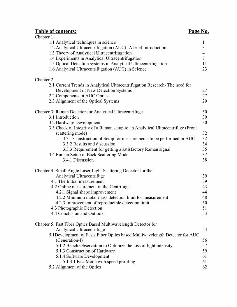
Table of contents: Page No. Chapter 1 1.1 Analytical techniques in science 1 1.2 Analytical Ultracentrifugation (AUC) -A brief Introduction 3 1.3 Theory of Analytical Ultracentrifugation 4 1.4 Experiments in Analytical Ultracentrifugation 7 1.5 Optical Detection systems in Analytical Ultracentrifugation 11 1.6 Analytical Ultracentrifugation (AUC) in Science 23 Chapter 2
2.1 Current Trends in Analytical Ultracentrifugation Research- The need for Development of New Detection Systems 27
2.2 Components in AUC Optics 27 2.3 Alignment of the Optical Systems 29
Chapter 3: Raman Detector for Analytical Ultracentrifuge 30 3.1 Introduction 30 3.2 Hardware Development 30
3.3 Check of Integrity of a Raman setup to an Analytical Ultracentrifuge (Front scattering mode) 32
3.3.1 Construction of Setup for measurements to be performed in AUC 32 3.3.2 Results and discussion 34 3.3.3 Requirement for getting a satisfactory Raman signal 35 3.4 Raman Setup in Back Scattering Mode 37 3.4.1 Discussion 38 Chapter 4: Small Angle Laser Light Scattering Detector for the
Analytical Ultracentrifuge 39 4.1 The Initial measurement 39 4.2 Online measurement in the Centrifuge 43 4.2.1 Signal shape improvement 44 4.2.2 Minimum molar mass detection limit for measurement 48 4.2.3 Improvement of reproducible detection limit 50 4.3 Photographic Detection 51 4.4 Conclusion and Outlook 53
Chapter 5: Fast Fiber Optics Based Multiwavelength Detector for Analytical Ultracentrifuge 54
5.1Development of Fasts Fiber Optics based Multiwavelength Detector for AUC (Generation-I) 56
5.1.2 Bench Observation to Optimize the loss of light intensity 57 5.1.3 Construction of Hardware 59 5.1.4 Software Development 61 5.1.4.1 Fast Mode with speed profiling 61 5.2 Alignment of the Optics 62

ii
5.3 Results 63 5.3.1 Time Domain Data 63 5.3.2 Radial Mode data 64 5.3.3 Speed profile data 64 5.4 Discussion 65
Chapter 6: Fasts Fiber Optics based Multiwavelength Detector for AUC (Generation-II) 68
6.1 Hardware Development 68 6.2 Software Development 70 6.3 Alignment of the Optics 77 6.4 Optics performance test 77 6.5 Measurement results to check the detector reliability 78 6.6 Conclusion of the first Phase of work for 2nd Generation Multiwavelength
Detector 81 6.7 Further Improvements of the 2nd Generation Detector 81 6.7.1 Alignment of the Optics 84 6.7.2 Optics Performance Test 85 6.7.3 Experimental Results 87 6.8 Discussion-2nd Generation Multiwavelength Detector 92 6.9 Third Generation Multiwavelength Detector 96
Chapter 7 7.1Conclusion 101 7.2 Detector Development in Analytical Ultracentrifuge-A future outlook 102
Appendix-I: Mechanical drawing of different parts used for the construction of the 2nd
generation Multiwavelength Optics 107 Appendix-II: Estimation of Construction cost for the 2nd generation Multiwavelength
Detector 110
Appendix-II: Alignment procedure for 2nd generation Multiwavelength Detector 111
Zusammenfassung 112 Popular Abstract 114 Symbols 115 Abbreviations 116 Acknowledgements 117 References 118
1
Chapter 1
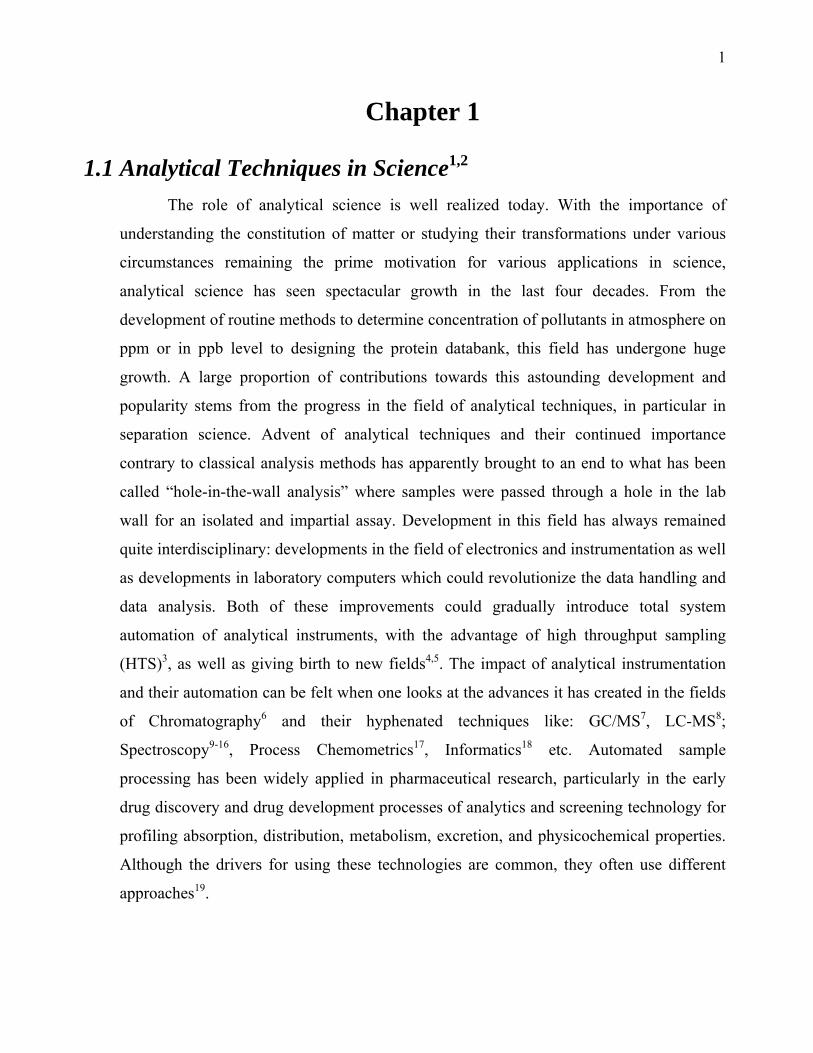
1.1 Analytical Techniques in Science1,2
The role of analytical science is well realized today. With the importance of
understanding the constitution of matter or studying their transformations under various
circumstances remaining the prime motivation for various applications in science,
analytical science has seen spectacular growth in the last four decades. From the
development of routine methods to determine concentration of pollutants in atmosphere on
ppm or in ppb level to designing the protein databank, this field has undergone huge
growth. A large proportion of contributions towards this astounding development and
popularity stems from the progress in the field of analytical techniques, in particular in
separation science. Advent of analytical techniques and their continued importance
contrary to classical analysis methods has apparently brought to an end to what has been
called “hole-in-the-wall analysis” where samples were passed through a hole in the lab
wall for an isolated and impartial assay. Development in this field has always remained
quite interdisciplinary: developments in the field of electronics and instrumentation as well
as developments in laboratory computers which could revolutionize the data handling and
data analysis. Both of these improvements could gradually introduce total system
automation of analytical instruments, with the advantage of high throughput sampling
(HTS)3, as well as giving birth to new fields4,5. The impact of analytical instrumentation
and their automation can be felt when one looks at the advances it has created in the fields
of Chromatography6 and their hyphenated techniques like: GC/MS7, LC-MS8;
Spectroscopy9-16, Process Chemometrics17, Informatics18 etc. Automated sample
processing has been widely applied in pharmaceutical research, particularly in the early
drug discovery and drug development processes of analytics and screening technology for
profiling absorption, distribution, metabolism, excretion, and physicochemical properties.
Although the drivers for using these technologies are common, they often use different
approaches19.

2
The importance of analytical science rose to its current level largely as a result of
contemporary development contemporary in the separation techniques. The extensive use
of chromatographic instruments (like HPLC or GC) in industry and other laboratories is
indicative of this. It is well known that the detection system in any separation technique
plays a crucial role and continuous efforts are made to improve upon these systems in
order to enhance its applicability of the techniques. The detection systems like visible and
UV spectrometers as non destructive methods or Iodine and Ammonia vapours to enhance
sensitivity to organic acids for detection on a TLC plate were used in former times. With
the advent of new technologies, separation techniques have been coupled with new
systems (optical detection as well as other hyphenated techniques) for the obvious reason
that this approach enriches the available analyte information. The ever increasing
popularity of orthogonal chromatography20 in combination with its multidimensional20,21
application leads to the realization of applicability of Multidetection systems in
fractionation techniques. Application of such strategies can give a better insight into a
complex analyte mixture under investigation by supplying information of the analyte
behaviour22 and allowing the determination of specific physicochemical parameters that
are characteristic of the technique. Recently, detection systems employing spectroscopic
techniques like Raman, FTIR and MS have come into picture. Other examples include
possible ESR detection for understanding aging process in living tissues23, and the use of
tandem TLC-HPTLC-MS contrary to their solo technique nowadays.
However, the development of new detection systems to separation techniques
usually focuses on chromatographic methods, and such application to other techniques
have so far been overlooked. Analytical Ultracentrifugation (AUC) is a powerful
fractionation technique that has supplied valuable information to biochemists and
biophysicists. With its implementation in the last century by Thé Svedberg24,25, this
technique has seen some spectacular development in instrumentation along with the
inception of new optical detection systems, such as absorbance, interference or Schlieren
optics. However, other detection systems can also be implemented to AUC. Such detection
systems include multiwavelength detection which can provide valuable information for
interacting macromolecular systems26 or information about the wavelength dependency of

3
particle size, a light scattering detector which can be used for online molar mass detection.
Also, it may also be mentioned that for the AUC detection systems, the inceptions of the
contemporary development in electronics or other related fields have not been so common.
It is clear in the history of developments of AUC that improvements in the detector
hardware have been neglected, in comparison to development of the data evaluation
software27-30. In the present work, effort has been made to fill this gap by introducing
adoptable developments from other area of science, towards improved detection
capabilities in AUC experiments.
1.2 Analytical Ultracentrifugation (AUC)-A brief introduction
An Analytical Ultracentrifuge (AUC) is a centrifuge that allows to spin a rotor at
accurately controlled speed and temperature, whilst allowing for the recording of the
concentration distribution of the sample at known times. In order to achieve rapid
sedimentation and to minimize diffusion, high angular velocities may be necessary. The
rotor of an analytical ultracentrifuge is typically capable at speeds up to 60,000 rpm. In
order to minimize frictional heating, and to minimize aerodynamic turbulence, the rotor is
usually spun in an evacuated chamber. It is also necessary for the instrumentation of an
AUC that the rotor be free of wobble and precession.
The power of the technique of AUC lies in the fact that the separation of solute
components can be achieved in the centrifugal field. The separation is based on molar
mass, density, shape and charge. This endows unique characteristics to this technique that
unlike in other fractionation techniques, the solute components do not interact with the
solvent in another phase. During an AUC experiment, it is necessary to monitor the
concentration gradient of sedimenting molecules, and this must be achieved using optics31
as physical contact with the sample is not possible. Thus, there remains the requirement of
designing ways to shine a beam of light through the sample in an AUC cell and use some
optical property of the solute to determine its distribution in the ultracentrifuge cell. The
optical properties of the solute currently exploited in existing common AUC detectors are
4
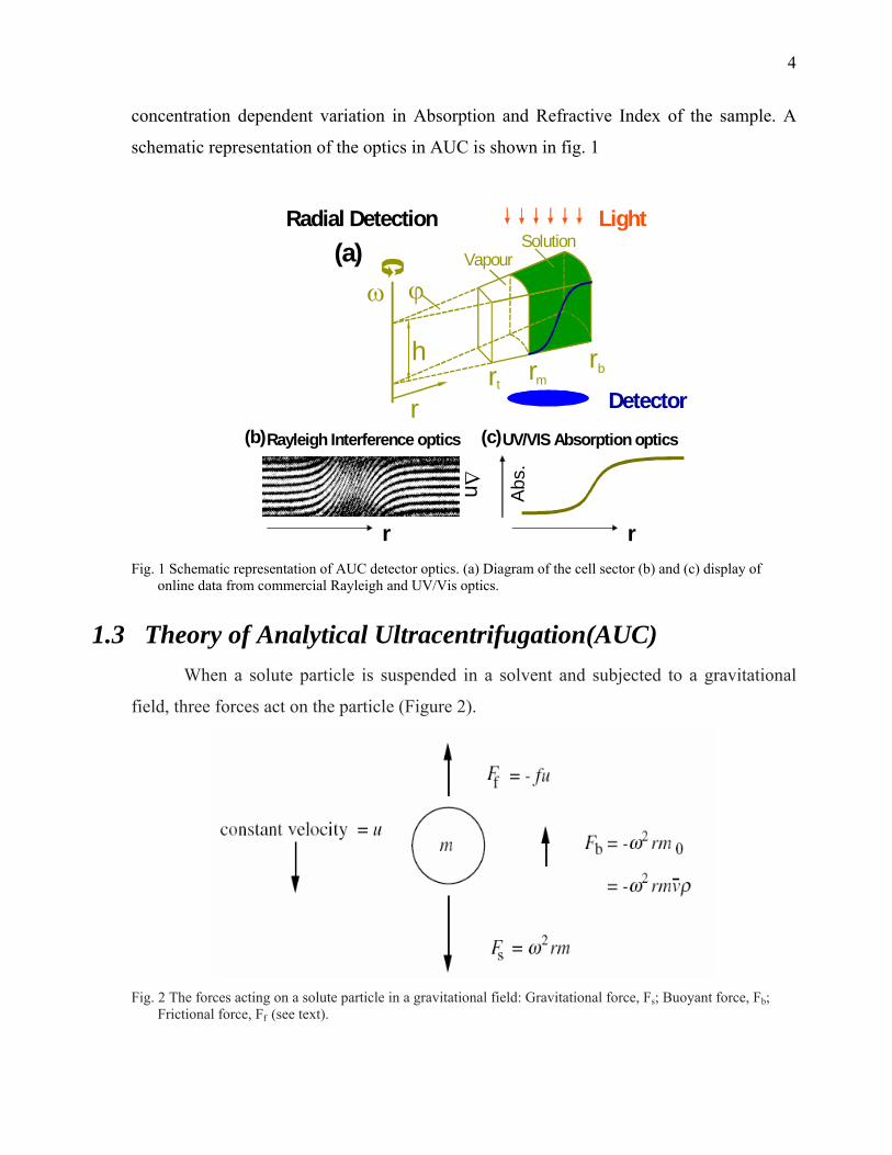
concentration dependent variation in Absorption and Refractive Index of the sample. A
schematic representation of the optics in AUC is shown in fig. 1
h
ϕ
rr r r
t m
VapourSolution
ω
b
Radial Detection
Rayleigh Interference optics UV/VIS Absorption optics∆n
Abs.
r r
Light
Detector
(a)
(b) (c)
Fig. 1 Schematic representation of AUC detector optics. (a) Diagram of the cell sector (b) and (c) display of
online data from commercial Rayleigh and UV/Vis optics.
1.3 Theory of Analytical Ultracentrifugation(AUC)
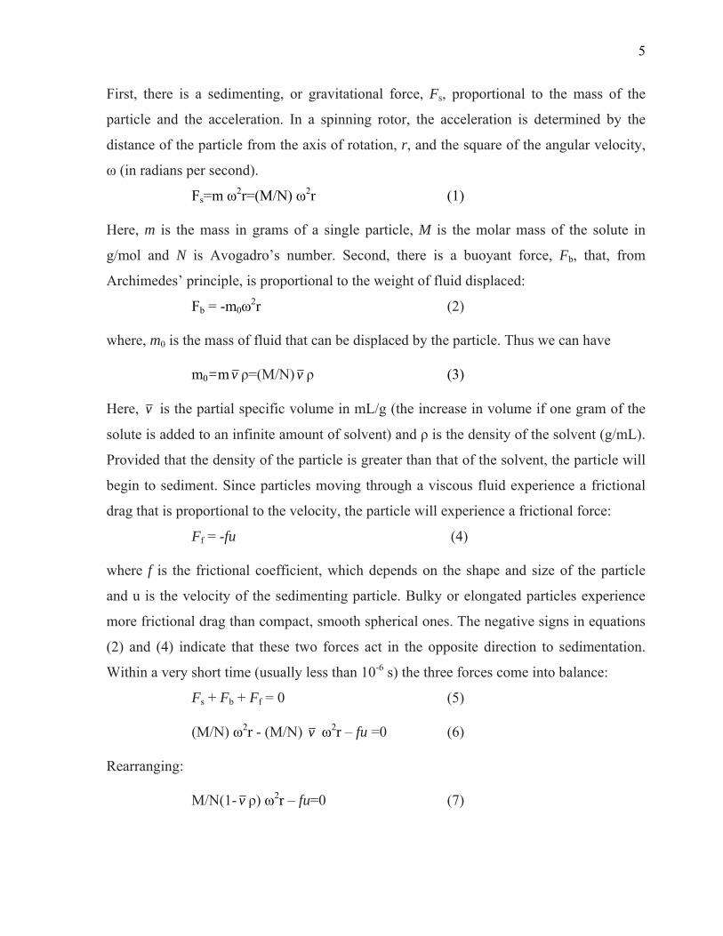
When a solute particle is suspended in a solvent and subjected to a gravitational
field, three forces act on the particle (Figure 2).
Fig. 2 The forces acting on a solute particle in a gravitational field: Gravitational force, Fs; Buoyant force, Fb;
Frictional force, Ff (see text).
5
First, there is a sedimenting, or gravitational force, Fs, proportional to the mass of the
particle and the acceleration. In a spinning rotor, the acceleration is determined by the
distance of the particle from the axis of rotation, r, and the square of the angular velocity,
ω (in radians per second).
Fs=m ω2r=(M/N) ω2r (1)
Here, m is the mass in grams of a single particle, M is the molar mass of the solute in
g/mol and N is Avogadro’s number. Second, there is a buoyant force, Fb, that, from
Archimedes’ principle, is proportional to the weight of fluid displaced:
Fb = -m0ω2r (2)
where, m0 is the mass of fluid that can be displaced by the particle. Thus we can have
m0=m v ρ=(M/N) v ρ (3)
Here, v is the partial specific volume in mL/g (the increase in volume if one gram of the
solute is added to an infinite amount of solvent) and ρ is the density of the solvent (g/mL).
Provided that the density of the particle is greater than that of the solvent, the particle will
begin to sediment. Since particles moving through a viscous fluid experience a frictional
drag that is proportional to the velocity, the particle will experience a frictional force:
Ff = -fu (4)
where f is the frictional coefficient, which depends on the shape and size of the particle
and u is the velocity of the sedimenting particle. Bulky or elongated particles experience
more frictional drag than compact, smooth spherical ones. The negative signs in equations
(2) and (4) indicate that these two forces act in the opposite direction to sedimentation.
Within a very short time (usually less than 10-6 s) the three forces come into balance:
Fs + Fb + Ff = 0 (5)
(M/N) ω2r - (M/N) v ω2r – fu =0 (6)
Rearranging:
M/N(1- v ρ) ω2r – fu=0 (7)
6
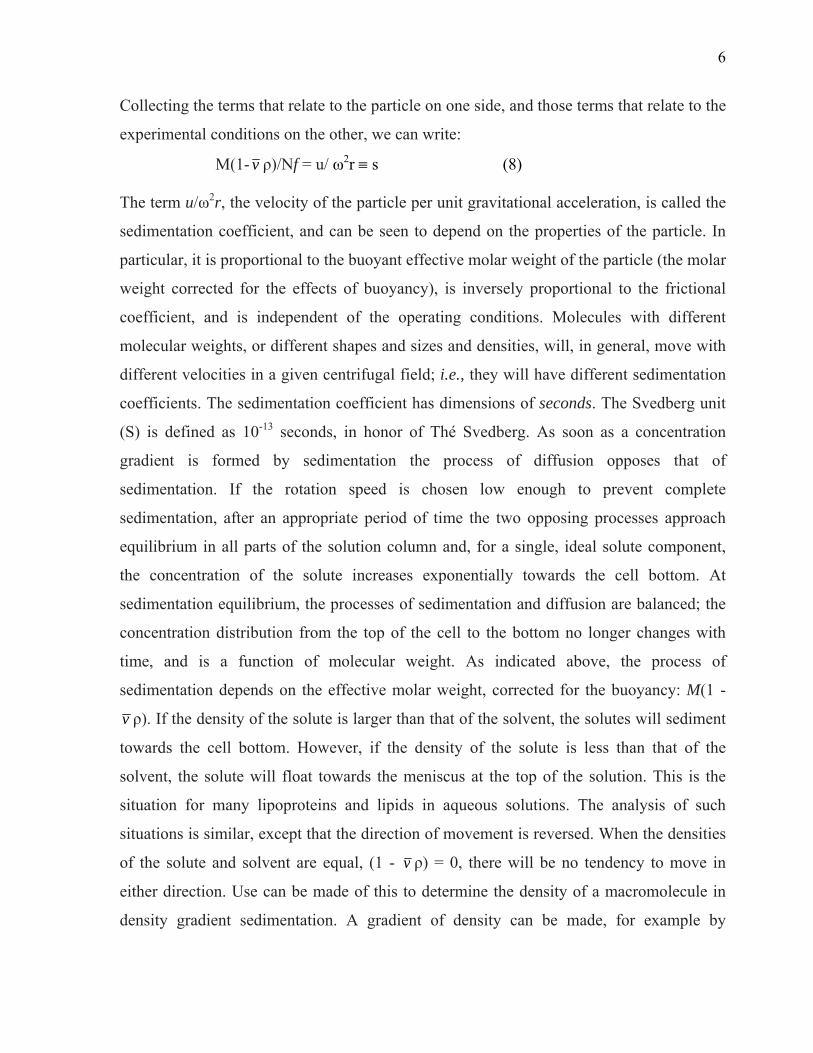
Collecting the terms that relate to the particle on one side, and those terms that relate to the
experimental conditions on the other, we can write:
M(1- v ρ)/Nf = u/ ω2r ≡ s (8) The term u/ω2r, the velocity of the particle per unit gravitational acceleration, is called the
sedimentation coefficient, and can be seen to depend on the properties of the particle. In
particular, it is proportional to the buoyant effective molar weight of the particle (the molar
weight corrected for the effects of buoyancy), is inversely proportional to the frictional
coefficient, and is independent of the operating conditions. Molecules with different
molecular weights, or different shapes and sizes and densities, will, in general, move with
different velocities in a given centrifugal field; i.e., they will have different sedimentation
coefficients. The sedimentation coefficient has dimensions of seconds. The Svedberg unit
(S) is defined as 10-13 seconds, in honor of Thé Svedberg. As soon as a concentration
gradient is formed by sedimentation the process of diffusion opposes that of
sedimentation. If the rotation speed is chosen low enough to prevent complete
sedimentation, after an appropriate period of time the two opposing processes approach
equilibrium in all parts of the solution column and, for a single, ideal solute component,
the concentration of the solute increases exponentially towards the cell bottom. At
sedimentation equilibrium, the processes of sedimentation and diffusion are balanced; the
concentration distribution from the top of the cell to the bottom no longer changes with
time, and is a function of molecular weight. As indicated above, the process of
sedimentation depends on the effective molar weight, corrected for the buoyancy: M(1 -
v ρ). If the density of the solute is larger than that of the solvent, the solutes will sediment
towards the cell bottom. However, if the density of the solute is less than that of the
solvent, the solute will float towards the meniscus at the top of the solution. This is the
situation for many lipoproteins and lipids in aqueous solutions. The analysis of such
situations is similar, except that the direction of movement is reversed. When the densities
of the solute and solvent are equal, (1 - v ρ) = 0, there will be no tendency to move in
either direction. Use can be made of this to determine the density of a macromolecule in
density gradient sedimentation. A gradient of density can be made, for example by
7
generating a gradient of concentration of an added solute such as sucrose or cesium
chloride from high concentrations at the cell bottom to lower values at the top. The
macromolecule will sediment if it is in a region of solution where the density is less than
its own. But macromolecules that find themselves in a region of higher density will begin
to float. Eventually, the macromolecules will form a layer at that region of the cell where
the solvent density is equal to their own: the buoyant density.
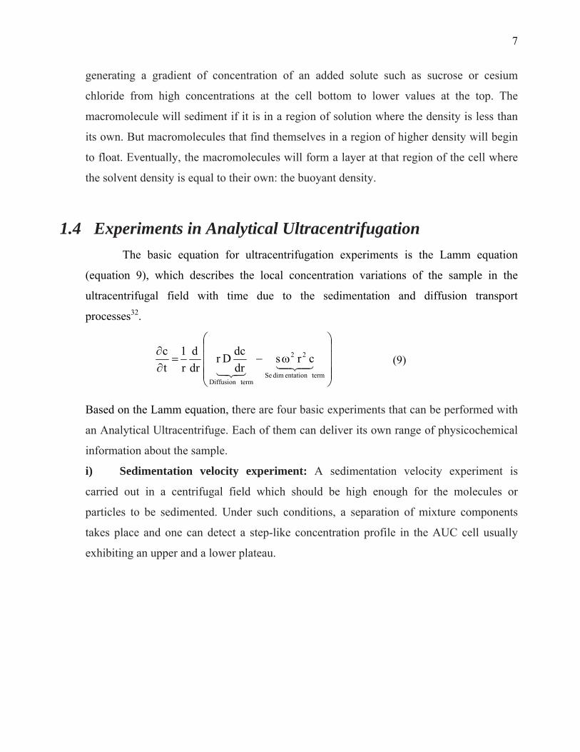
1.4 Experiments in Analytical Ultracentrifugation The basic equation for ultracentrifugation experiments is the Lamm equation
(equation 9), which describes the local concentration variations of the sample in the
ultracentrifugal field with time due to the sedimentation and diffusion transport
processes32.
⎟⎟⎟⎟
⎠
⎞
⎜⎜⎜⎜
⎝
⎛
ω−=∂∂
43421321 termentationdimSe
22
termDiffusion
crsdrdcDr
drd
r1
tc
(9)
Based on the Lamm equation, there are four basic experiments that can be performed with
an Analytical Ultracentrifuge. Each of them can deliver its own range of physicochemical
information about the sample.
i) Sedimentation velocity experiment: A sedimentation velocity experiment is
carried out in a centrifugal field which should be high enough for the molecules or
particles to be sedimented. Under such conditions, a separation of mixture components
takes place and one can detect a step-like concentration profile in the AUC cell usually
exhibiting an upper and a lower plateau.
8
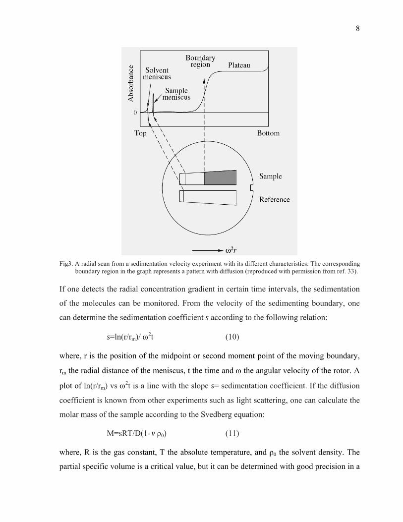
Fig3. A radial scan from a sedimentation velocity experiment with its different characteristics. The corresponding
boundary region in the graph represents a pattern with diffusion (reproduced with permission from ref. 33).
If one detects the radial concentration gradient in certain time intervals, the sedimentation
of the molecules can be monitored. From the velocity of the sedimenting boundary, one
can determine the sedimentation coefficient s according to the following relation:
s=ln(r/rm)/ ω2t (10)
where, r is the position of the midpoint or second moment point of the moving boundary,
rm the radial distance of the meniscus, t the time and ω the angular velocity of the rotor. A
plot of ln(r/rm) vs ω2t is a line with the slope s= sedimentation coefficient. If the diffusion
coefficient is known from other experiments such as light scattering, one can calculate the
molar mass of the sample according to the Svedberg equation:
M=sRT/D(1- v ρ0) (11)
where, R is the gas constant, T the absolute temperature, and ρ0 the solvent density. The
partial specific volume is a critical value, but it can be determined with good precision in a

9
density oscillation tube if enough sample material is available. In biochemistry, often only
a very small amount of sample is available so that this measurement can present a
problem, however different workarounds are also available, such as the calculation of v
from the amino acid composition.
In general, sedimentation velocity experiments offer a good possibility for the rapid
determination of molar mass but also of equilibrium constants of interacting systems
which is especially advantageous for unstable systems which can not be subjected to
sedimentation equilibrium experiments due to the danger of sample degradation during the
experiment34. There are many procedures to determine the sedimentation coefficient from
sedimentation velocity data. Of these, the Moving Boundary method35 or Van Holde-
Weischet method36,37 are the best known. The moving boundary method allows evaluation
of the diffusion coefficient from the spreading of the boundary during the experiment,
allowing calculation of M38. In the Van Holde-Weischet method the diffusion broadening
of boundaries is eliminated by selecting a fixed number of data points from one
experimental scan that are evenly spaced between the baseline and the plateau. This is
followed by calculation of an apparent sedimentation coefficient s* for each of the data
points, which when plotted versus the inverse root of the runtime, yielding the typical van
Holde-Weischet plot. Another method for the evaluation of s from the sedimentation data
is the Time derivative method39,40,41 that determines the time derivative of the radial scans
acquired at different times. This method serves better for treatment of data for multimodal
distribution of solutes, which is a general case for polymers, and works by determining the
differential form of G(s) the g(s).
ii) Sedimentation equilibrium experiments: In contrast to the sedimentation
velocity experiments, a sedimentation equilibrium experiment is carried out at a
centrifugal field so that the solute under interest does not sediment completely. Here, the
sedimentation of the sample is balanced by back diffusion according to Fick`s law caused
by the established concentration gradient. After the equilibrium between these two
transport processes is achieved, an exponential concentration gradient is formed in the
ultracentrifuge cell. Therefore, the sedimentation equilibrium analysis is based on solid
10
thermodynamics. The time of equilibrium attainment considerably depends on the column
height of the solution42 so that short column techniques, with solution columns of about
1mm, can be employed wherever a rapid equilibrium (within 1-2 hours or less) is
desired43. The concentration gradient contains information about the molar mass of the
sample, the second osmotic virial coefficient, or interaction constants in case of interacting
systems independently of the shape of the molecule. An advantage is that the detection of
the concentration gradient is possible without disturbing the chemical equilibrium even of
weak interactions. Various procedures exist for the evaluation of sedimentation
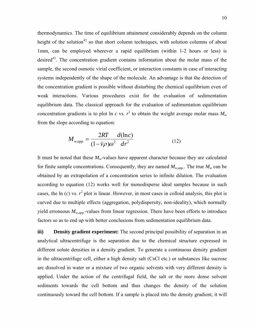
equilibrium data. The classical approach for the evaluation of sedimentation equilibrium
concentration gradients is to plot ln c vs. r2 to obtain the weight average molar mass Mw
from the slope according to equation:
22.,)(ln
)1(2
rdcd
vTRM appw ωρ−
= (12)
It must be noted that these Mw-values have apparent character because they are calculated
for finite sample concentrations. Consequently, they are named Mw,app.. The true Mw can be
obtained by an extrapolation of a concentration series to infinite dilution. The evaluation
according to equation (12) works well for monodisperse ideal samples because in such
cases, the ln (c) vs. r2 plot is linear. However, in most cases in colloid analysis, this plot is
curved due to multiple effects (aggregation, polydispersity, non-ideality), which normally
yield erroneous Mw,app.-values from linear regression. There have been efforts to introduce
factors so as to end up with better conclusions from sedimentation equilibrium data.
iii) Density gradient experiment: The second principal possibility of separation in an
analytical ultracentrifuge is the separation due to the chemical structure expressed in
different solute densities in a density gradient. To generate a continuous density gradient
in the ultracentrifuge cell, either a high density salt (CsCl etc.) or substances like sucrose
are dissolved in water or a mixture of two organic solvents with very different density is
applied. Under the action of the centrifugal field, the salt or the more dense solvent
sediments towards the cell bottom and thus changes the density of the solution
continuously toward the cell bottom. If a sample is placed into the density gradient, it will

11
sediment /float to a position where its density matches that of the gradient. In case of a
mixture, this leads to a banding of the components due to their chemical structure/density.
As this experiment was not of main concern in the work carried out, the detail of this
method will not be discussed. More information about this can be found in literature44.
iv) Synthetic Boundary experiment: In a synthetic boundary experiment, changes of
a boundary between solution and solvent with time are observed at low centrifugal fields
where no sedimentation of the sample occurs. Such experiments require special cells
where the solvent is layered upon the solution column under the action of a certain
centrifugal field. This is achieved by capillaries which connect the solvent compartment of
the cell with the solution compartment and which allow a flow at a certain hydrostatic
pressure. The details of these experiments are also available in literature45.
An alternative approach of zone or band sedimentation approach was developed
by Vinograd et al46. In this method, macromolecules are transferred, on the initiation of
centrifugation, through a channel from a small well in the centrifuge cell to the sample
sector solution which contains a solution of greater density than the macromolecular
solution. A self-generated density gradient caused by the diffusion of small molecules
between the macromolecular lamella and the main liquid column prevents convection,
thereby stabilizing the macromolecules in a sedimenting band or zone. Band centrifugation
was applied successfully for characterization of DNA and RNA with CsCl, NaCl, D2O as
the primary small solute for generating the self-diffusion density gradients for nucleic
acids and band stabilization47. It has the potential advantage of working with low sample
quantity (1/20 th of that conventional sedimentation velocity experiment uses) and distinct
separation of the sedimenting species. Software has also been developed to work out the
sedimentation coefficients from the band data48.
1.5 Optical Detection systems in Analytical Ultracentrifugation
As already discussed, the present detection systems in AUC rely on absorption or
Refractive Index variation of the sample with solute concentration. All existing detection
systems for AUC have a similar setup, where light from a source is guided through the cell

12
sector containing the sample for measurement, and the light of interest is detected by a
photosensor. However, an improved detection system can always be designed to meet the
demand of increasing potential of AUC. An overview of existing detection system in AUC
is discussed here.
i) UV/Vis Absorption Optics: This detection system of AUC is quite simple. The
commercial version of this system, the Beckman Optima XL-A instrument49, uses a UV-
enhanced xenon flashlamp as the light source, which is projected from a 1mm circular
aperture which makes the light to impinge on a holographically generated, toroidally
curved diffraction grating especially designed for this application. This grating is
aberration-corrected so that the system has a nominal 2 nm band pass between 200 nm and
800 nm with very low stray light. The grating is rotated by a precision gear train to select
or scan a wavelength in this range. This diffraction grating is additionally blazed by ion
bombardment to intensify the first-order light efficiency in the UV range, which also
decreases chromatic stray light. Light which is not passing out of the exit aperture of the
monochromator is absorbed by a series of semi-reflective and non-reflective absorbing
filters to prevent this light at the exit of the monochromator. Stray light levels at 210nm
are typically 0.1%. Light leaving the diffraction grating then impinges on an 8% reflector
that reflects this light back to a solid-state detector, mounted at the virtual focal point of
the monochromator system. Thus the detector monitors the intensity of light incident on
the sample in the cell assembly. This intensity value, in conjunction with the transmitted
intensity value measured by the PM tube at the detection end of the system, is used to
normalize the pulse-to-pulse variation in the light intensity emitted from the flashlamp.
This is necessary as the reference and the sample sectors in the cell are measured
separately. The exit aperture of the monochromator prevents illumination of the sector not
being measured. This eliminates spectral stray light and the resulting non-linearity in
absorption measurement. Light passing through the mid-plane of the sector being
measured is then refocused by the camera lens assembly into the plane of a slit above the
PM tube. This slit and lens assembly is moved so that they undergo motion directly
proportional to the image size of the cell. The active area of the PM tube is larger than this

13
distance and, therefore, remains stationary. A schematic description of this optical system
is shown in the figure below:
Fig. 4 Absorbance Optics system in commercial Beckmann Optima XL-A (with permission from ref.33)
There have been quite a few contributions from various researchers for the
instrumentation of the absorption optics. In the oldest version of this detection system,
photographic plates were used. In some modifications with photographic plates as
detectors, efforts were made in several ways to illuminate the cell and to grab photographs
of sedimenting analyte50. This was followed by the use of photoelectric scanner, although
in their simplest form these do little more than replace the photographic plate by a
photoelectric detector (e.g a PMT), the most highly developed of which was introduced by
Lamers, Putney, Steinberg and Schachman (1963)31. In later developments, researchers

14
used a scanner based on a video camera50. In one significant development introduced by
Flossdorf51 with the introduction of parabolic mirror based collimator optics in the
absorbance optical system exhibited a pronounced enhancement of detected UV/Vis
intensity.
ii) Interference Optics: The fundamental principle of this detection system relies on the fact
that the velocity of light passing through a region of higher refractive index is decreased.
The optical setup consists of monochromatic light that passes through two fine parallel
slits, one above each sector of a double-sector cell containing, respectively, a sample of
solution and a sample of solvent in dialysis equilibrium. Light waves emerging from the
entrance slits and passing through the two sectors undergo interference when combined by
a focusing lens and yield a band of alternating light and dark “fringes.” When the
refractive index in the sample compartment is higher than in the reference, the sample
wave is retarded relative to the reference wave. This causes the positions of the fringes to
shift vertically in proportion to the concentration difference relative to that of some
reference point which is usually the meniscus air/solution. If the concentration of the
reference point, crF, is known, the concentration at any other point can be obtained:
cr = crF +a∆j (13) where ∆j is the vertical fringe shift, and a is a constant relating concentration to fringe
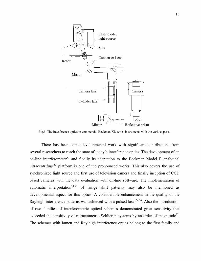
shift. In interference optics, the Rayleigh interferometer in the analytical ultracentrifuge
produces a cell image in which the concentration at each radial position is presented as the
vertical displacement of a set of equally-spaced horizontal fringes. A schematic depiction
of the optics as adopted for a commercial Ultracentrifuge is shown below:
15
Laser diode, light source
Slits
Rotor Condenser Lens
Mirror
Camera lens
Mirror
Cylinder lens
Reflective prism
Camera
Fig.5 The Interference optics in commercial Beckman XL series instruments with the various parts.
There has been some developmental work with significant contributions from
several researchers to reach the state of today’s interference optics. The development of an
on-line interferometer52 and finally its adaptation to the Beckman Model E analytical
ultracentrifuge53 platform is one of the pronounced works. This also covers the use of
synchronized light source and first use of television camera and finally inception of CCD
based cameras with the data evaluation with on-line software. The implementation of
automatic interpretation54,55 of fringe shift patterns may also be mentioned as
developmental aspect for this optics. A considerable enhancement in the quality of the
Rayleigh interference patterns was achieved with a pulsed laser54,56. Also the introduction
of two families of interferometric optical schemes demonstrated great sensitivity that
exceeded the sensitivity of refractometric Schlieren systems by an order of magnitude57.
The schemes with Jamen and Rayleigh interference optics belong to the first family and

16
those with Lebedev, Bringdahl, and Beutelspacher belong to second family58. The path of
light beam in these two shift interferometric patterns is shown below:
Fig.6 Schematic path of beams in the shift interferometers of the two families of interferometric optics. ‘a’ and
‘b’ refers to the first and second families as mentioned in the text. ‘c’ presents the resulting interference patterns. 1 and 2 are two systems of light beams shifted from one another; 3 is the reference cell sector with a solvent, and 4 is the sample cell; n and n0 are refractive indexes of the solution and the solvent respectively (reproduced with permission from ref. 58)
All this experience has been combined in the present commercial interferometric
optics with Rayleigh interferometer. Apart from the commercial one, the Lebedev
interferometric59 optics is used by some researchers. This is a polarizing interferometer
with three main advantages (that can provide the user with a better image of the process
within the cell): 1) high sensitivity 2) absence of optical error for high speed experiments
3) the system is free of astigmatic optical elements. It has been constructed for use on a
MOM AUC platform. The optical scheme (ref. Fig, 7) consists of a mercury lamp (1) as
the light source which passes through a monochromatizing device, and is focused by a lens
(2) on the point diaphragm (3). With the aid of another lens (4) it travels further as a
parallel beam. The beam is polarized with a polaroid (6) (with optical axis oriented at an
angle of 45° to the radial direction) and separated into two beams by a birefringent plate
(7) made, for example from Iceland spar. Consequently, the interacting beams in the cell
are mutually shifted from one another by the distance a (spar twinning), the direction of
the shift being normal to the plane of the solution-solvent interface. After passing a half-
wave plate (λ/2) (mica plate rotating the planes of polarization of both beams by 90°) and
Polaroid (13), crossed with the first (6), make it possible to observe the interference
pattern of the two polarized beams. A telescopic system of lenses (10, 11) transforms one
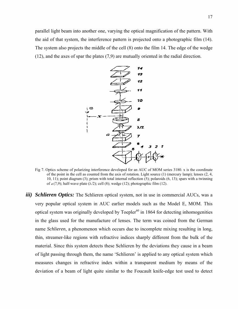
17
parallel light beam into another one, varying the optical magnification of the pattern. With
the aid of that system, the interference pattern is projected onto a photographic film (14).
The system also projects the middle of the cell (8) onto the film 14. The edge of the wedge
(12), and the axes of spar the plates (7,9) are mutually oriented in the radial direction.
Fig 7. Optics scheme of polarizing interference developed for an AUC of MOM series 3180. x is the coordinate
of the point in the cell as counted from the axis of rotation. Light source (1) (mercury lamp); lenses (2, 4, 10, 11); point diagram (3); prism with total internal reflection (5); polaroids (6, 13); spars with a twinning of a (7,9); half-wave plate (λ/2); cell (8); wedge (12); photographic film (12).
iii) Schlieren Optics: The Schlieren optical system, not in use in commercial AUCs, was a
very popular optical system in AUC earlier models such as the Model E, MOM. This
optical system was originally developed by Toepler60 in 1864 for detecting inhomogenities
in the glass used for the manufacture of lenses. The term was coined from the German
name Schlieren, a phenomenon which occurs due to incomplete mixing resulting in long,
thin, streamer-like regions with refractive indices sharply different from the bulk of the
material. Since this system detects these Schlieren by the deviations they cause in a beam
of light passing through them, the name ‘Schlieren’ is applied to any optical system which
measures changes in refractive index within a transparent medium by means of the
deviation of a beam of light quite similar to the Foucault knife-edge test used to detect
18
aberrations in lenses and mirrors. This optical system has developed slowly from quite
simple forms to its present complexity. In the AUC cell, as there is a concentration
gradient, the light passing through a region in the cell is deviated radially and the Schlieren
optical system converts the radial deviation of light into a vertical displacement of an
image at the camera. This displacement is proportional to the concentration gradient. The
Schlieren image is thus a measure of the concentration gradient, dc/dr, as a function of
radial distance, r. The change in concentration relative to that at some specified point in
the cell (e.g. the meniscus) can be determined at any other point by integration of the
Schlieren profile. Much of the existing literature on sedimentation, particularly
sedimentation velocity, has been obtained with the use of this optical system. The earliest
Schlieren system was described by Thovert (1902) and on the basis of his system, various
workers developed AUC Schlieren systems (e.g. Tanner61 1927). A sample design was
reported by Lamm62 (1937), in which a transparent scale was mounted close to, but not
coincident with, the cell, and is photographed through the cell. The image of the scale was
distorted by gradients of the refractive index in the cell, and by careful measurement of
this distortion it was possible to deduce the variation of dn/dr with r within the cell. A
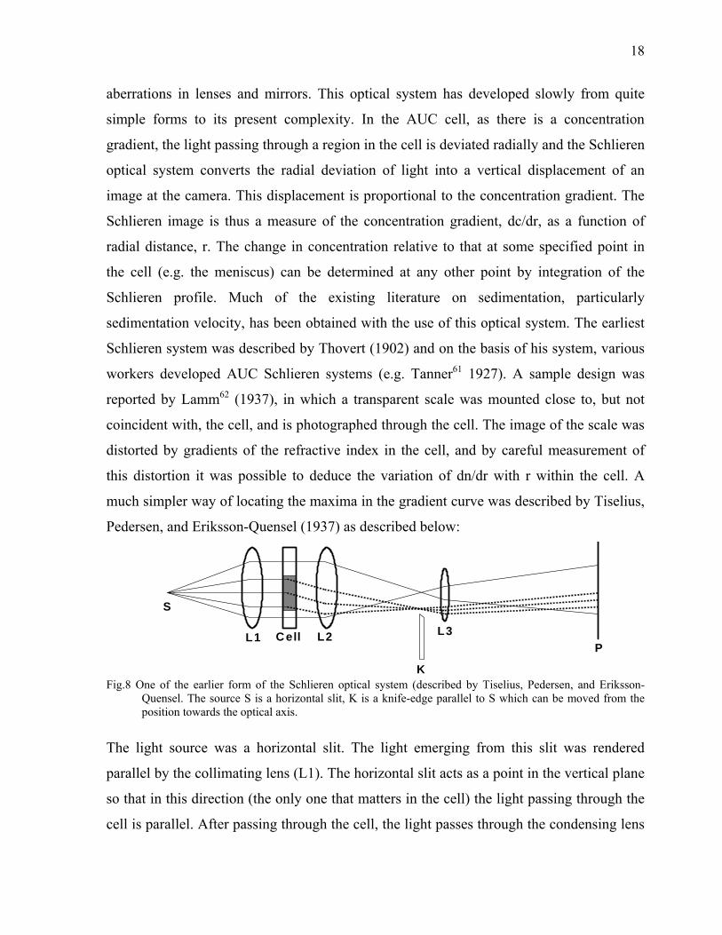
much simpler way of locating the maxima in the gradient curve was described by Tiselius,
Pedersen, and Eriksson-Quensel (1937) as described below:
S
L1 C ell L2
K
L3P
Fig.8 One of the earlier form of the Schlieren optical system (described by Tiselius, Pedersen, and Eriksson-
Quensel. The source S is a horizontal slit, K is a knife-edge parallel to S which can be moved from the position towards the optical axis.
The light source was a horizontal slit. The light emerging from this slit was rendered
parallel by the collimating lens (L1). The horizontal slit acts as a point in the vertical plane
so that in this direction (the only one that matters in the cell) the light passing through the
cell is parallel. After passing through the cell, the light passes through the condensing lens
19
(L2), which forms an image of the light source in its focal plane. Light passing through the
parts of the cell with no gradient refractive index forms am image on the optical axis.
However, rays of light that are deviated by passing through a concentration gradient in the
cell produce an image displaced from the optical axis (shown in dotted line in the figure)
The light rays pass through a camera lens L3 which forms an image of the cell on a
photographic plate or ground-glass screen P.
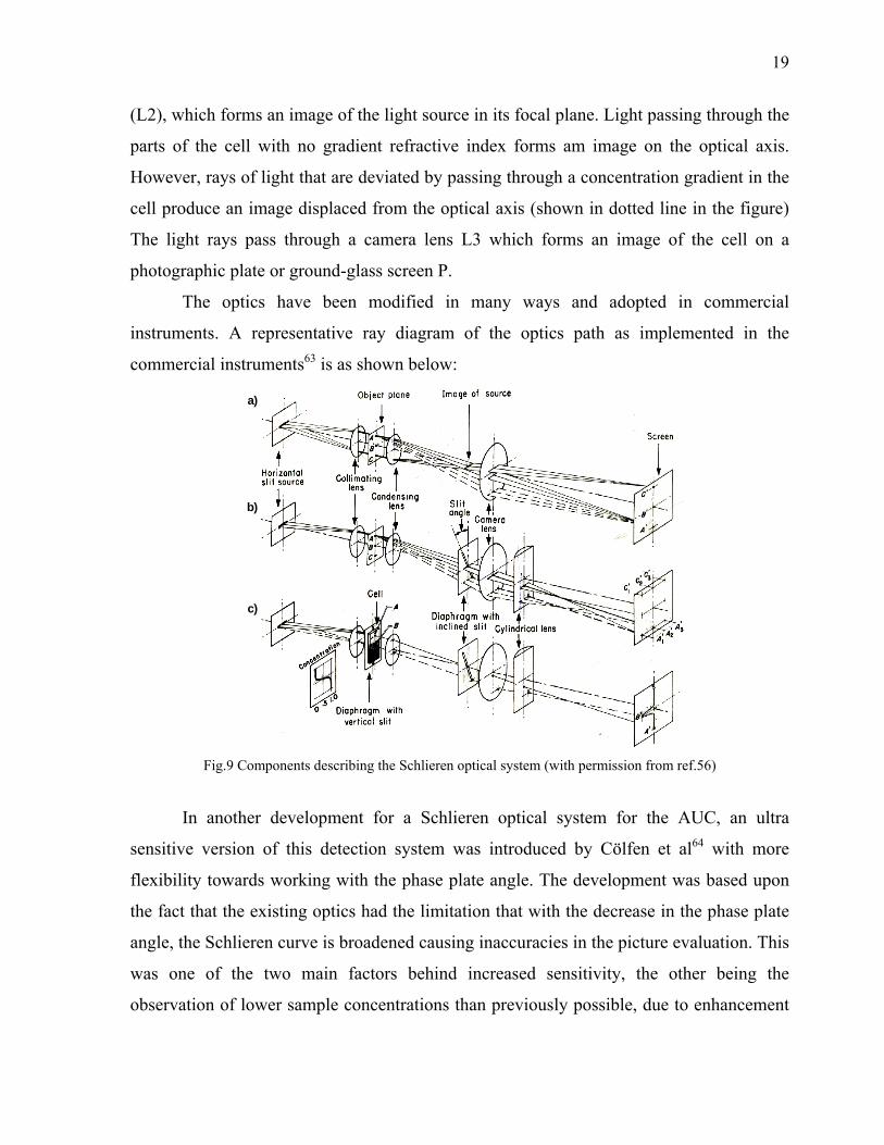
The optics have been modified in many ways and adopted in commercial
instruments. A representative ray diagram of the optics path as implemented in the
commercial instruments63 is as shown below:
a)
b)
c)
Fig.9 Components describing the Schlieren optical system (with permission from ref.56)
In another development for a Schlieren optical system for the AUC, an ultra
sensitive version of this detection system was introduced by Cölfen et al64 with more
flexibility towards working with the phase plate angle. The development was based upon
the fact that the existing optics had the limitation that with the decrease in the phase plate
angle, the Schlieren curve is broadened causing inaccuracies in the picture evaluation. This
was one of the two main factors behind increased sensitivity, the other being the
observation of lower sample concentrations than previously possible, due to enhancement
20
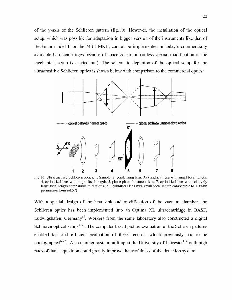
of the y-axis of the Schlieren pattern (fig.10). However, the installation of the optical
setup, which was possible for adaptation in bigger version of the instruments like that of
Beckman model E or the MSE MKII, cannot be implemented in today’s commercially
available Ultracentrifuges because of space constraint (unless special modification in the
mechanical setup is carried out). The schematic depiction of the optical setup for the
ultrasensitive Schlieren optics is shown below with comparison to the commercial optics:
Fig 10. Ultrasensitive Schlieren optics. 1. Sample, 2. condensing lens, 3.cylindrical lens with small focal length,
4. cylindrical lens with larger focal length, 5. phase plate, 6. camera lens, 7. cylindrical lens with relatively large focal length comparable to that of 4, 8. Cylindrical lens with small focal length comparable to 3. (with permission from ref.57)
With a special design of the heat sink and modification of the vacuum chamber, the
Schlieren optics has been implemented into an Optima XL ultracentrifuge in BASF,
Ludwigshafen, Germany65. Workers from the same laboratory also constructed a digital
Schlieren optical setup66,67. The computer based picture evaluation of the Sclieren patterns
enabled fast and efficient evaluation of these records, which previously had to be
photographed68-70. Also another system built up at the University of Leicester114 with high
rates of data acquisition could greatly improve the usefulness of the detection system.
21
IV) Fluorescence Detection: Apart from the usual, above described detection systems,
Fluorescence detection can also be applied in AUC with a recent and modern version
available for the XL-A AUC71. The Fluorescence detection system provides the advantage
of working with trace quantities of material, down to pM concentration level, a unique
feature that is not possible with any other optical system. In the old version of this system,
development was performed on the basis of a Spinco Model E72. The optical system used a
scanning microscope in which only a very small area of the sample is illuminated by an
electron beam or a laser beam, and the intensity of the emitted or reflected radiation is
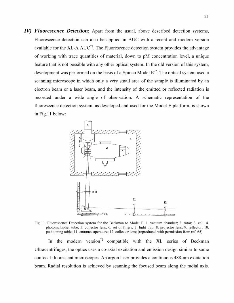
recorded under a wide angle of observation. A schematic representation of the
fluorescence detection system, as developed and used for the Model E platform, is shown
in Fig.11 below:
4
567
1
23
8
910
1112
Fig 11. Fluorescence Detection system for the Beckman to Model E. 1. vacuum chamber; 2. rotor; 3. cell; 4.
photomultiplier tube; 5. collector lens; 6. set of filters; 7. light trap; 8. projector lens; 9. reflector; 10. positioning table; 11. entrance aperature; 12. collector lens; (reproduced with permission from ref. 65)
In the modern version72 compatible with the XL series of Beckman
Ultracentrifuges, the optics uses a co-axial excitation and emission design similar to some
confocal fluorescent microscopes. An argon laser provides a continuous 488-nm excitation
beam. Radial resolution is achieved by scanning the focused beam along the radial axis.
22
Detection of the fluorescence signal uses a co-axial, front-face optical configuration to
reduce inaccuracies in the concentration caused by inner filter effects. A high-speed data
acquisition system allows the fluorescence intensity to be monitored continuously and at a
sufficiently high angular resolution that at any radial position the intensities from all the
samples may be acquired at each revolution. The fluorescence detector is capable of
detecting concentrations as low as 300 pM for fluorescein-like labels.
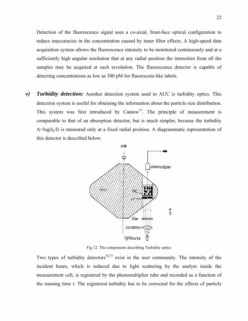
v) Turbidity detection: Another detection system used in AUC is turbidity optics. This
detection system is useful for obtaining the information about the particle size distribution.
This system was first introduced by Cantow73. The principle of measurement is
comparable to that of an absorption detector, but is much simpler, because the turbidity
A=log(I0/I) is measured only at a fixed radial position. A diagrammatic representation of
this detector is described below:
Fig 12. The components describing Turbidity optics
Two types of turbidity detectors74,75 exist in the user community. The intensity of the
incident beam, which is reduced due to light scattering by the analyte inside the
measurement cell, is registered by the photomultiplier tube and recorded as a function of
the running time t. The registered turbidity has to be corrected for the effects of particle
23
size and refractive index by application of MIE theory to yield the particle concentration
of a particular size. In the newly constructed version in the same laboratory, a narrow
continuous beam of a laser diode (λ =670nm) is used as the light source and a fast
photodiode is used as light detector76.
1.6 Analytical Ultracentrifugation (AUC) in Science
Analytical Ultracentrifugation (AUC) has proven to be a valuable tool for the study
of macromolecular systems since its invention by Svedberg77. Earlier studies by Svedberg
were confined to the study of proteins and particle size characterization of gold colloids,
however, the importance of the technique could soon be felt in several areas where
macromolecular characterization is of prime importance. There are numerous examples of
information derived by one of the four basic experiments or combinations thereof using an
ultracentrifuge. The impact of AUC is well discussed in many reviews that cover different
aspects of the technique78-84.
i) Application of AUC in analysis of colloids: The application of analytical
ultracentrifugation for the determination of particle sizes and their distributions to was
already realized by the pioneers of this technique, because sedimentation velocity
experiments provide a sensitive fractionation due to particle sizes or molar masses85-88. It is
relatively straightforward to convert a sedimentation coefficient distribution to a parameter
that can be determined from Ultracentrifugation experiments: using the equation
s = ln( r / rm ) / ω2t for every data point (a) ri (if a radial scan is obtained at a specified
time) or (b) ti (if a concentration detection at a specified radius has been performed as a
function of time) to a particle size distribution. Assuming the validity of Stoke’s law (e.g.
if the sample is spherical), the following derivative of the Svedberg equation is obtained
ρρη−
=2
18 ii
sd (14)
where di is the particle diameter corresponding the sed. Coefficient to si , ρ2 is the density
of the sedimenting particle (including solvent/polymer etc. adhering to the sample), and
24
η the solvent viscosity. If the particles are not spherical, only the hydrodynamically
equivalent diameter is obtained unless form factors are applied if the axial ratio of the
particles is known from other sources like e.g. TEM. The conversion of the sedimentation
coefficient distribution to a particle size distribution highly relies on the knowledge of the
density of the sedimenting particle. Thus the determination of the particle size from
Analytical ultracentrifugation is quite robust and rapid, with comfortable statistical
accuracy (since every sedimenting particle is detected) in contrast to transmission electron
microscopy (TEM) which delivers information about the particle shape but often suffers
from the drawbacks due to drying artifacts. Determination of particle size distribution
from TEM images requires counting hundreds or thousands of particles, although this
problem has been partly diminished by the advent of commercially available picture
evaluation algorithms. A combination of TEM, AUC and X-ray diffraction techniques can
provide a complete insight into a colloidal system89. AUC in combination with electron
microscopy in its various forms can be considered the most powerful characterization
approach for the determination of particle size distributions and particle morphologies
known to date. There have been many examples that illustrate the fractionation power of
the AUC for latex90,91and especially for inorganic colloids92.
ii) Application for Investigating Biological systems: AUC has proven to be a widely
used method for the characterization of self-association and heteroassociation of
macromolecules in solution. Such interaction was predominantly studied with
sedimentation equilibrium experiments which were further supported by the determination
by X-ray diffraction crystal structure.
Nowadays, sedimentation velocity is also increasingly applied for the
determination of interaction constants. Examples have shown how both sedimentation
velocity and the sedimentation equilibrium experiment can be used to investigate in detail
the self-association of insulin analogues under formulation conditions93 for
pharmaceuticals. The implications for the pharmacokinetic and pharmacodynamic
responses of these insulin analogues were discussed, and it was suggested that
25
sedimentation analysis can help in developing improved rapid-acting insulin therapies, and
furthermore that AUC is one of the few techniques where analysis can be performed on the
formulation and result in quantification of the protein interactions under those
conditions94. An excellent example of the application of sedimentation equilibrium
analysis to characterize protein ligand and receptor interactions is mentioned in the work
of Philo and his colleagues95. Sedimentation equilibrium analysis at varying rotor speeds
could reveal the very weak binding constant of receptor and protein. Various studies
indicating the study for characterization of receptor protein ligand interactions can also be
found96,97. There have been reported applications of a wide range of applications of the use
of sedimentation equilibrium to characterize protein oligomerization including the
dimerization of human growth hormone by zinc98 or self-association of biglycan99.
AUC has also found application in the study of biopharmaceutical stability and
homogeneity. This step is one of the most important steps in the development of
pharmaceuticals; the degradation products of biopharmaceuticals often include aggregates
and fragments. One possible way to identify these degradation products is to determine
their average molecular weights by using sedimentation equilibrium analysis26,100. For
highly purified and homogeneous molecules, the average molecular weights for the pure
and non-self-associated macromolecules under ideal conditions should be very similar to
the monomer molecular weights. On the other hand, for macromolecules that have
undergone aggregation or fragmentation, the apparent average molecular weights under
ideal conditions will vary from the monomer molecular weights. The purity of
biopharmaceuticals can also be determined by the sedimentation velocity analysis. Several
sedimentation velocity methods have been developed to determine the distribution of
protein species, the most useful one being van Holde and Weischet analysis101,102. This
approach is well documented to provide a rigorous test of sample homogeneity103 and has
been successfully utilized to study the homogeneity of macromolecules104,105. A different
method, with the extrapolation based on the time derivative of concentration distribution
has also found application in the identification of impurities in macromolecules106,107. This
method has been used in combination with other methods viz. SDS, polyacrylamide gel
26
electrophoresis and gel permeation chromatography, to help determine the purity and
homogeneity of macromolecules in solution108.
Another quite useful application area of AUC is the determination of the binding
affinity of protein interaction to biopharmaceuticals. This property of proteins is
thermodynamically reconcilable and hence the sedimentation equilibrium experiment has
proved to be the most rigorous method for its determination33. The sedimentation
equilibrium method has been successfully and extensively used by many workers to
investigate the association constants of interacting systems 27,109,110. AUC has also been
extensively used by biochemists and biophysicists for the study of biopolymers with
respect to solution conformation, conformational changes, association behaviour, and
homologous and heterologous interactions (including the thermodynamics)111,112.
Apart from the above mentioned applications AUC has also been prominently used
to study other bio macromolecular systems such as polysaccharides113.

27
Chapter 2
2.1 Current Trends in Analytical Ultracentrifugation (AUC) Research - The Need for Development of New Detection Systems
Developments in AUC have been of interest to several research groups worldwide.
This includes the development of AUC to investigate novel systems, improvement of data
evaluation methodologies to solve biophysical questions etc. The least developed, yet most
vital component in AUC is the detection system. This is primarily due to the hardware
development time necessary for detection systems. Final adaptation of a new system to an
existing AUC platform needs design and construction of new mechanical and electronic
parts which are often time consuming. However, to meet the experimental demand of
sensitive, faster, and increasingly online data generation, the development of new
detection system has become essential. Also, the present detection systems for AUC can
not supply a satisfactory amount of chemical information. In his visionary paper,
Mächtle114 mentioned about the future requirement of AUC detection systems with the
need to implement a light scattering, IR or Raman detection system to generate data
enriched with more chemical information. Such optical systems can be developed and
designed for simultaneous use with the present absorption and Rayleigh interference
optics.
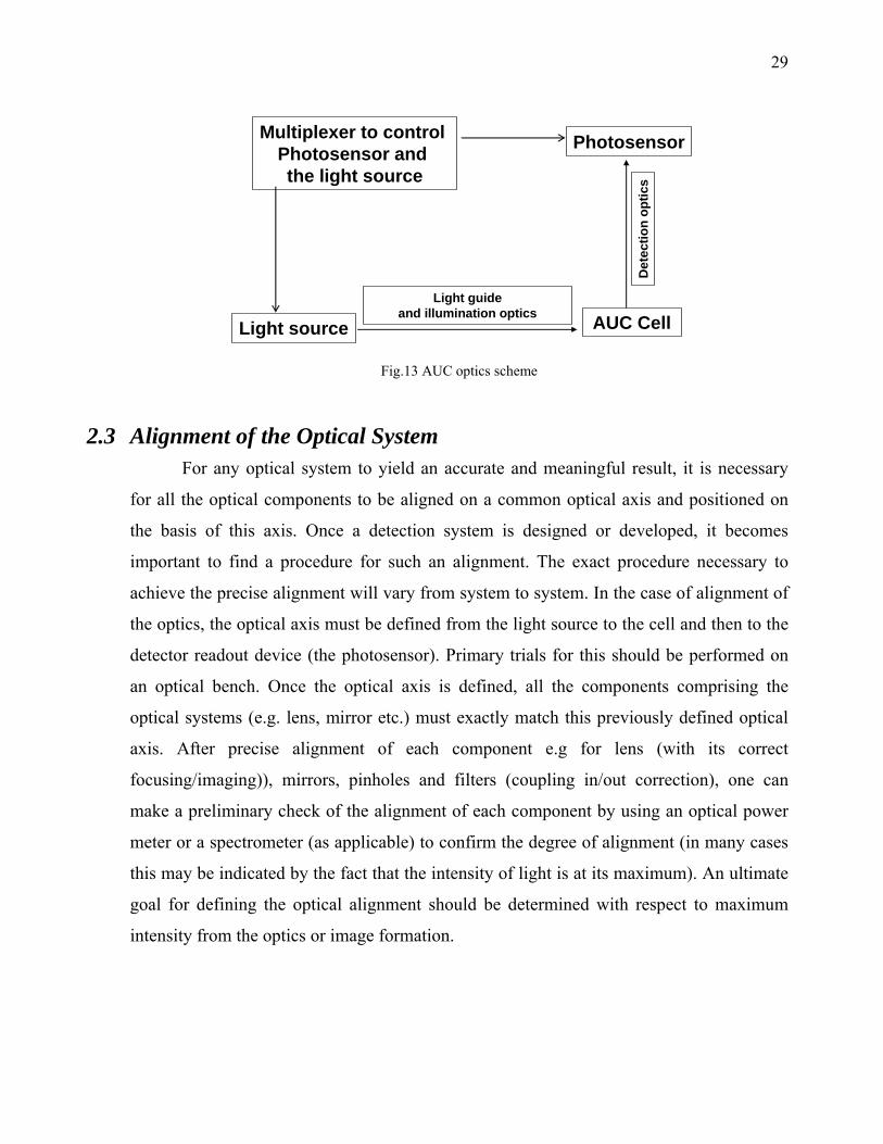
2.2 Components in AUC Optics AUC optics comprises a light source for illumination of the cell followed by other
optical components (e.g lenses, mirrors) and finally a photosensor to collect the light
emerging out of the cell. When designing the optics for AUC, an adaptable system is
necessary to address the different parameter of various experiments. Unlike the selection
of the light source, selection of other components are difficult as they may depend upon
various factors such as aberration effects115 (e.g. spherical aberration, monochromatic off-
axis aberration, chromatic aberration etc.). In the selection of the photosensor, there are
28
also choices available and one can decide on the basis of the need, for enhanced
sensitivity, faster response, or a compromise between these two. A photomultiplier tube,
for example can well serve for high sensitivity, while a photodiode can result in faster
response but less sensitivity. Examples include: photographic plates (in today’s context
with the use of cameras), vacuum devices like a Photomultiplier tube (PMT),
semiconductor devices (a photodiode) or gaseous photodetectors. Light from the source
uses illumination optics to make it incident on the cell sector which after emerging from
the cell sector is collected by detection optics and finally passed to the photosensor. The
primary requirement of the illumination optics design is for light to be drawn into the
AUC vacuum chamber as the detector should collect data from a sedimenting sample in
ultracentrifugal field in this chamber. In order to achieve this, optical fibers can be used.
There are many types of commercially available optical fibers so that one can make a
selection on the basis of the required working wavelengths (e.g. if the fiber needs to guide
light for UV light, a quartz fiber will have to be used) or enhanced photo flux (e.g. for
enhanced intensity a larger cladding/ core diameter fiber can be used). For the design of
illumination and detection optics, components like lenses, mirrors or prisms can be used.
In order to maximize the performance of the detector, operation of the lamp and the
photosensor needs to be controlled. This requirement arises as synchronization of the light
source with the rotor movement is necessary. The desired situation is that light should
enter the photosensor only when the sample is in the path of optics. With today’s
technology, one can implement this synchronization by triggering the detector read out
device (the photosensor) along with the light source, when the sample cell comes into this
path. Use of suitable multiplexer technology can enable this, and various research based
on the development of multiplexers for AUC116-119 has developed such a system. In the
present XL series of AUCs, the multiplexer signal can be input from the XL-I boards
directly and can be used for triggering signal of the optics (see Fig.13). These signals
come as TTL (Transistor Transistor Logic) signals and can be used by software as
information source of rotor movement. However, the XL preparative platform requires
conversion of the rotor signal obtained from the XL board to a TTL signal.
29
Light source AUC CellLight guide
and illumination optics
Det
ectio
n op
tics
PhotosensorMultiplexer to control Photosensor and the light source
Fig.13 AUC optics scheme
2.3 Alignment of the Optical System For any optical system to yield an accurate and meaningful result, it is necessary
for all the optical components to be aligned on a common optical axis and positioned on
the basis of this axis. Once a detection system is designed or developed, it becomes
important to find a procedure for such an alignment. The exact procedure necessary to
achieve the precise alignment will vary from system to system. In the case of alignment of
the optics, the optical axis must be defined from the light source to the cell and then to the
detector readout device (the photosensor). Primary trials for this should be performed on
an optical bench. Once the optical axis is defined, all the components comprising the
optical systems (e.g. lens, mirror etc.) must exactly match this previously defined optical
axis. After precise alignment of each component e.g for lens (with its correct
focusing/imaging)), mirrors, pinholes and filters (coupling in/out correction), one can
make a preliminary check of the alignment of each component by using an optical power
meter or a spectrometer (as applicable) to confirm the degree of alignment (in many cases
this may be indicated by the fact that the intensity of light is at its maximum). An ultimate
goal for defining the optical alignment should be determined with respect to maximum
intensity from the optics or image formation.

30
Chapter 3 A Raman Detector for Analytical Ultracentrifuge
3.1 Introduction
Raman Spectroscopy is a well known technique, often used complementary to
infrared spectroscopy, and is capable of providing quantitative analysis and detailed
information about molecular structure. The importance of this technique has been well
realized for investigating a wide variety of samples ranging from the molecular changes
while studying ultra fast reaction dynamics of proteins120 or protein ligand interactions121
to polymer studies122 and inorganic complexes in solution2. Unlike IR spectroscopy,
Raman spectroscopy provides informations about symmetric molecular vibrations and
allows one to obtain spectral information in aqueous solution. This property makes the
technique a quite valuable tool for biochemists and also for the analysis of polymers and
colloids as different components in a mixture could be chemically characterized. Thus,
combination of Raman data for a fractionated sample in a centrifugal field will supply
chemists with valuable information from a sample mixture as different components in a
mixture could be chemically characterized while simultaneously obtaining the chemical
group-dependent concentration information. Although there has been quite an
advancement for the Raman instrumentation with new technologies e.g. with CCD
detection, the high cost of the instrumental setup is often a constraint. However, one can
consider the building of a Raman setup coupled to an Ultracentrifuge by assembling only
commercially available components123, and this was the initial motivation for constructing
a Raman detection system.
3.2 Hardware Development As the first step it was necessary to construct an adoptable Raman optics setup for
AUC. Therefore, it was decided to make an overview of commercial products for which
possibility for adaptation to AUC would be possible. The following setup considered
likely to yield optimum data quality if adapted to AUC was envisaged:
31
1. Fiber optics based Raman probe for data sampling in back scattering mode:
Working with a fiber optics based probe allowing light guiding inside the AUCvacuum
chamber.
2. Raman probe of focal length 3cm: This was decided on the basis of the fact that the
Raman probe will have to be kept at a distance away from the sample in the spinning
rotor while we can get optimum signal quality.
3. Application of pulsed laser: A pulsed laser can well serve the purpose of working
with short exposure time for a spinning sample in conjunction with a detector that can
be triggered allowing for multi-cell operation.
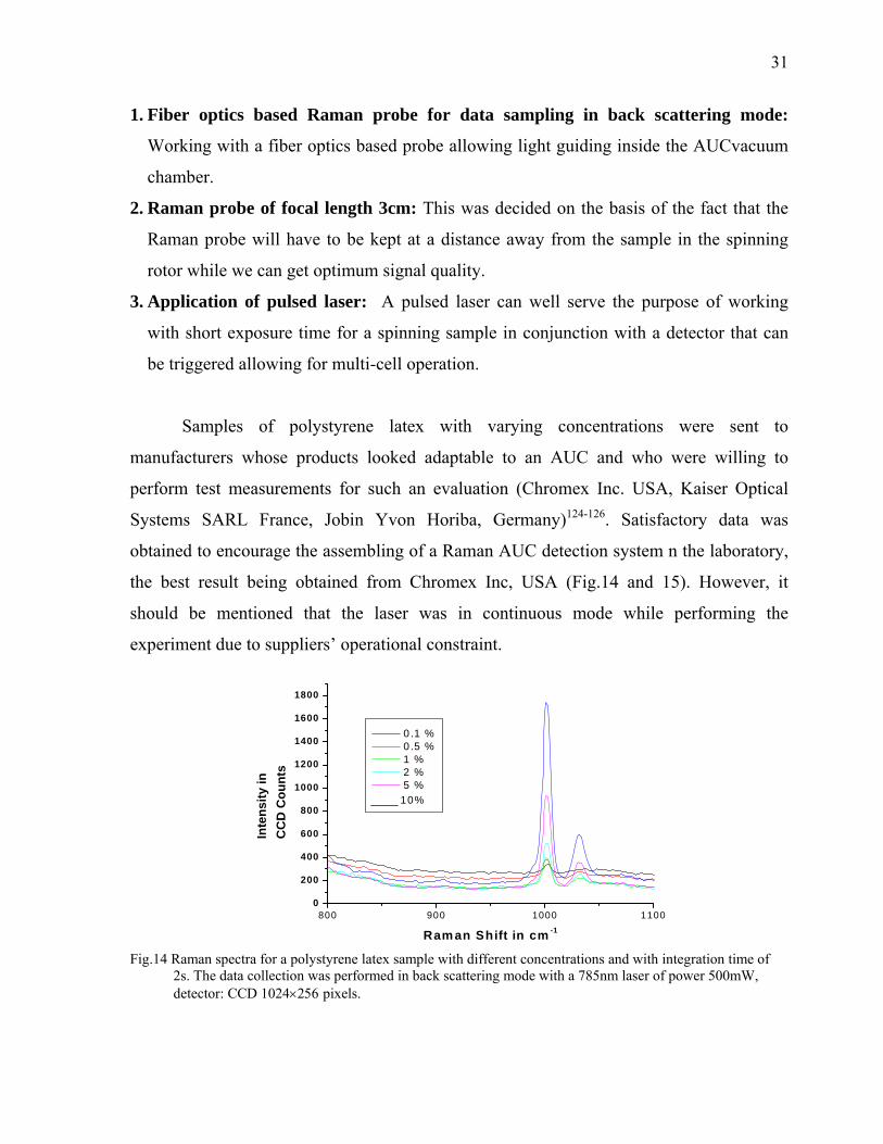
Samples of polystyrene latex with varying concentrations were sent to
manufacturers whose products looked adaptable to an AUC and who were willing to
perform test measurements for such an evaluation (Chromex Inc. USA, Kaiser Optical
Systems SARL France, Jobin Yvon Horiba, Germany)124-126. Satisfactory data was
obtained to encourage the assembling of a Raman AUC detection system n the laboratory,
the best result being obtained from Chromex Inc, USA (Fig.14 and 15). However, it
should be mentioned that the laser was in continuous mode while performing the
experiment due to suppliers’ operational constraint.
800 900 1000 11000
200
400
600
800
1000
1200
1400
1600
1800
Ram an Shift in cm -1
0 .1 % 0 .5 % 1 % 2 % 5 %
Inte
nsity
inC
CD
Cou
nts
10%
Fig.14 Raman spectra for a polystyrene latex sample with different concentrations and with integration time of
2s. The data collection was performed in back scattering mode with a 785nm laser of power 500mW, detector: CCD 1024×256 pixels.

32
0 500 1000 1500 2000 2500
-20
0
20
40
60
80
100
Inte
nsity
Raman Shift
10%
0 500 1000 1500 2000 2500-40
-20
0
20
40
60
Inte
nsity
Raman Shift
5%
0 500 1000 1500 2000 2500
-20
0
20
40
60
Inte
nsity
Raman Shift
2%
0 500 1000 1500 2000 2500-20
0
20
40
60
80
Inte
nsi
ty
Raman Shift
1%
0 500 1000 1500 2000 2500
-20
0
20
40
60
80
Inte
nsity
Raman Shift
0.5%
0 500 1000 1500 2000 2500-40
-20
0
20
40
60
80
100
Inte
nsity
Raman Shift
0.1%
Fig. 15. Raman signal observed for different concentrations of a Polystyrene latex with integration time 0.1s.
Similar instrumental configuration as in fig. 13.
The data from the commercial instrument (Chromex Inc) showed linearity in
response in the 2s integration time. However, the results looked quite inferior in very low
integration time, the 0.1% concentration with 2s integration time was almost at the noise
level. For AUC measurements this is not a satisfactory situation as this concentration does
not corresponds to the lowest detection limit of AUC. Furthermore, this integration time
for AUC experiments is not realistic for which an integration time in the ms range is
required. Also the very high cost of the setup ($110,878 in Nov. 2003) looks to be a prime
constraint. Thus we decided to try a possible Raman setup for AUC with facilities in hand,
to check for the integrity of such an AUC detection system.
3.3 Check of Integrity of a Raman Setup to an Analytical Ultracentrifuge (Front scattering mode)
3.3.1 Construction of Setup for measurements to be performed in AUC As a first test for a Raman setup to be adaptable to an AUC, it was decided to work
with optics in front scattering mode. This was because of the fact that for such a setup
hardware components were available which could be constructed on the existing
preparative XL-centrifuge platform in hand. The following components were procured to
perform a first check on a real AUC setup:
i) Laser: CompassTM 315M (obtained from BASF-AG)

33
Wavelength: 532nm, Power: ~20mW
Laser Source: Diode Pumped Nd:YAG
The laser was equipped with a Schäfter + Kirchhoff two fiber system that ends with a
single mode fiber with polarization maintained on both sides FC-APC (8° angled polish)
connectors, mode field diameter 4 µm, NA: 0.11.
ii) Spectrometer: Spectrapro 500i (Acton Research) with software “Scancontrol
Spectroscopy Plus”. The spectrometer is equipped with a TE cooled CCD
camera (Obtained from the Interface department, MPI-Golm).
iii) Optical fibers: 600 micron patch fiber UV/Vis (Ocean optics, The Netherlands)
iv) Other Optical elements: one 90° Prism, Biconvex lens (f=20.6mm, 20mm and
10mm) all from Linos, Göttingen, Germany.
In order to work with the above facility the following setup was applied (fig.16). However,
due to hardware constraints, in the preliminary set-up the measurements had to be
performed while keeping the centrifuge door open to feed in the fibers. The maximum
working speed is 3000 rpm in such a situation.
6
7
8
Fig.16 Schematic of the Raman detector setup: (1) 600 micron patch fiber UV/Vis (Ocean optics), (2) The
collimating lens system (self built), f= 20.6mm biconvex, (3) 90° Quartz Prism, (4) Converging lens to focus laser to the cell sector f = 20 mm biconvex, (5) Laser (6) Biconvex lens (f=10mm) (7) Edge filter (8) Spectrometer.

34
3.3.2 Results and discussion: Gold colloid and polystyrene latex samples were selected to observe the signal
quality of the setup. The sample selection was made on the basis of the high intensity of
Raman scattering peak of these samples since the rotation of the rotor will diminish the
signal intensity to a large extent. However, from a low speed of 1000 rpm no Raman
signal could be observed. With a standstill rotor and the sample directly in front of the
Laser, very weak Raman signal from the Polystyrene sample (for 5% Polystyrene latex
sample, peak position at~1000cm-1) could be observed (fig 17).
600 900 1200 1500 1800 2100
0
200
400
600
800
1000
Inte
nsity
in
CC
D c
ount
s
Raman Shift in cm-1
Raman Spectra of 5% Polystyrene sample(data from commercial instrument)
Signal for Polystyrene
600 900 1200 1500 1800 2100200
400
600
800
1000
Inte
nsity
in C
CD
Cou
nts
Raman Shift in cm-1
Very weak polystyrenesignal
Raman spectra for 5% Polystyrene sample(setup adapted to cetrifuge)
Fig.17. Signal from a Polystyrene latex sample (5%in water) Signal intensity was very weak with the setup adapted to the centrifuge (5s integration time with 3 acquisitions, standstill rotor).
Similar results with very weak Raman signal were also obtained for Gold colloid
sample. Raman spectrum recorded with the setup for Gold colloid is shown below:
Fig.18 Raman spectrum of Gold colloid sample recorded with the setup (30s integration, 3 acquisitions). The very high background signal (the other peak, aside from the sample which come from the background, air, solvent etc.) shows that front scattering mode should not be a preferred mode. The higher intensity of the background signal in blank is due to lower turbidity of the solution compared to the gold colloid sample. With less turbid sample, more of incident radiation can pass through the sample and finally more intensity arrives at the detector, hence the contribution to background signal is higher.
1500 2250 3000 3750
0
15000
30000
45000
60000
75000
Blank
1500 2250 3000 3750
300
450
600
750
900 Gold Colloid
Sam ple Peak

35
Even varying the recording parameters, sufficient signal intensity of the spectra could
not be observed. Thus it was concluded that the required Raman signal for adoption to
AUC would not be possible working with the present setup. Possibly, a 20mW laser may
not be sufficiently powerful to generate an observable Raman signal, however, the huge
contribution from the background, the signal being ~1/3 of the background in every case,
is also quite discouraging.
3.3.3 Requirement for getting a satisfactory Raman signal
Loss of light due to the Optical setup:
One possible reason for the very weak signal intensity from our setup could be that
the intensity of light at the detector was not optimal. Many coupling positions exist in the
setup where loss of light is inevitable. Thus as a next step, it was decided to check for the
loss of light intensity at different positions in the optics where coupling was performed.
Figure 19 summarizes the loss of light at these positions. Measurement in loss of intensity
was performed with an optical power meter, collecting the light directly from each
position with the help of a fiber.
Laser
Collimating lens with SMA adopter (~20%loss)
Prism(10% loss)
Spectrometer
Vacuum feed through(~10%loss)
Lenses and filter assemblyLoss:~20%
Fig.19 The different coupling points in the optics showing the amount of light intensity lost from light source to each position. A total loss of ~60% incident light intensity was observed.
From the amount of light loss in the above in description, the loss of 10% light due
to the vacuum feed through could be regained with the use of penetrating type feed
through, instead of receptacle type ones, as this removes the necessity to use an extra fiber
36
coupling. However, with the present setup the other losses could not be overcome due to
the time constraint and necessity of major modifications to the hardware mechanics of the
heat sink. Therefore, a ~60% loss of light intensity from the incident light to the point of
insertion to the spectrometer was concluded. The loss of ~20% light intensity before and
after the filter may not be correct as for measuring this loss, the filter had to be removed.
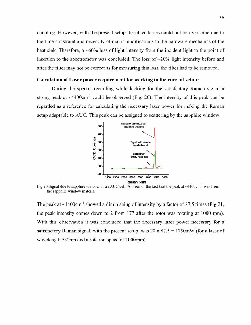
Calculation of Laser power requirement for working in the current setup:
During the spectra recording while looking for the satisfactory Raman signal a
strong peak at ~4400cm-1 could be observed (Fig. 20). The intensity of this peak can be
regarded as a reference for calculating the necessary laser power for making the Raman
setup adaptable to AUC. This peak can be assigned to scattering by the sapphire window.
1500 2000 2500 3000 3500 4000 4500 5000200
300
400
500
600
700
800
CC
D C
ount
s
Raman Shift
Signal for an empty cell (sapphire window)
Signal with sample inside the cell
Signal from empty rotor hole
Fig.20 Signal due to sapphire window of an AUC cell. A proof of the fact that the peak at ~4400cm-1 was from
the sapphire window material.
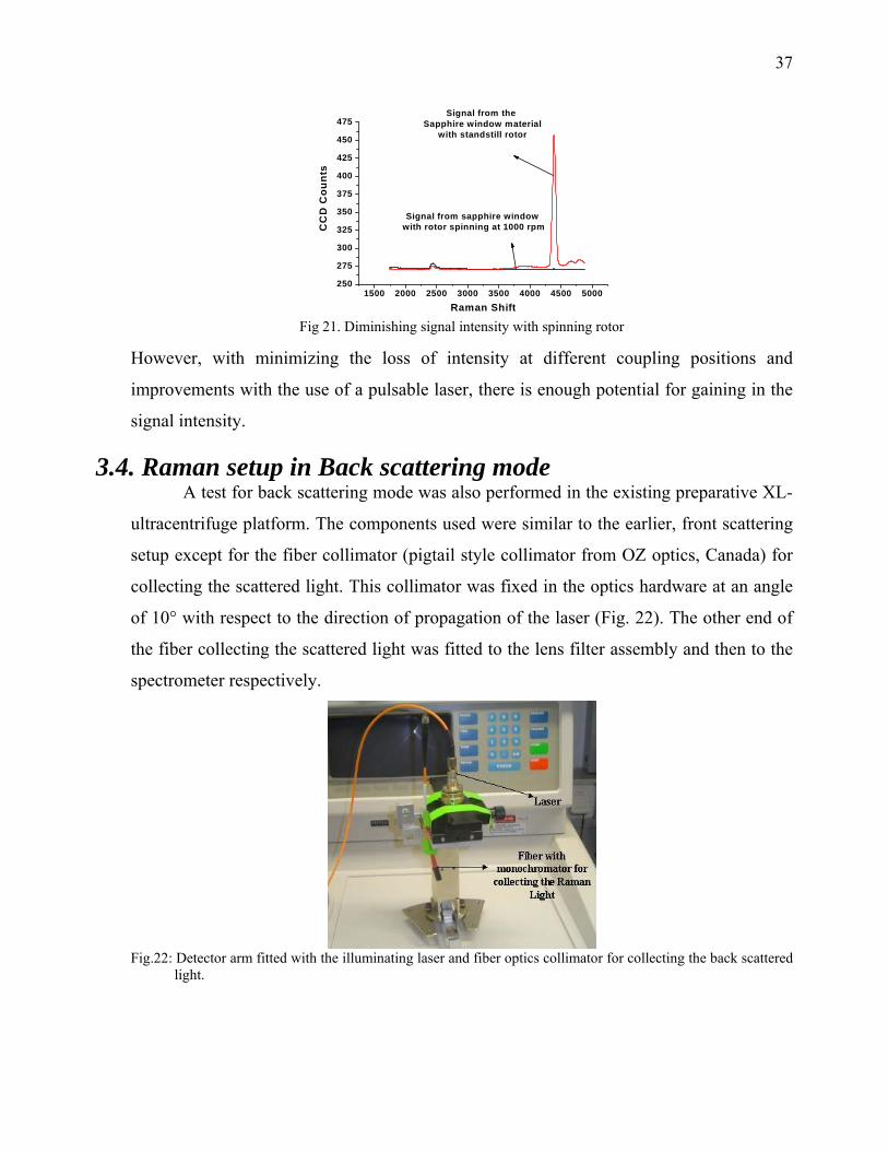
The peak at ~4400cm-1 showed a diminishing of intensity by a factor of 87.5 times (Fig.21,
the peak intensity comes down to 2 from 177 after the rotor was rotating at 1000 rpm).
With this observation it was concluded that the necessary laser power necessary for a
satisfactory Raman signal, with the present setup, was 20 x 87.5 = 1750mW (for a laser of
wavelength 532nm and a rotation speed of 1000rpm).
37
1500 2000 2500 3000 3500 4000 4500 5000250
275
300
325
350
375
400
425
450
475
CC
D C
ount
sRaman Shift
Signal from the Sapphire window material
with standstill rotor
Signal from sapphire window with rotor spinning at 1000 rpm
Fig 21. Diminishing signal intensity with spinning rotor
However, with minimizing the loss of intensity at different coupling positions and
improvements with the use of a pulsable laser, there is enough potential for gaining in the
signal intensity.
3.4. Raman setup in Back scattering mode A test for back scattering mode was also performed in the existing preparative XL-
ultracentrifuge platform. The components used were similar to the earlier, front scattering
setup except for the fiber collimator (pigtail style collimator from OZ optics, Canada) for
collecting the scattered light. This collimator was fixed in the optics hardware at an angle
of 10° with respect to the direction of propagation of the laser (Fig. 22). The other end of
the fiber collecting the scattered light was fitted to the lens filter assembly and then to the
spectrometer respectively.
Fig.22: Detector arm fitted with the illuminating laser and fiber optics collimator for collecting the back scattered
light.
38
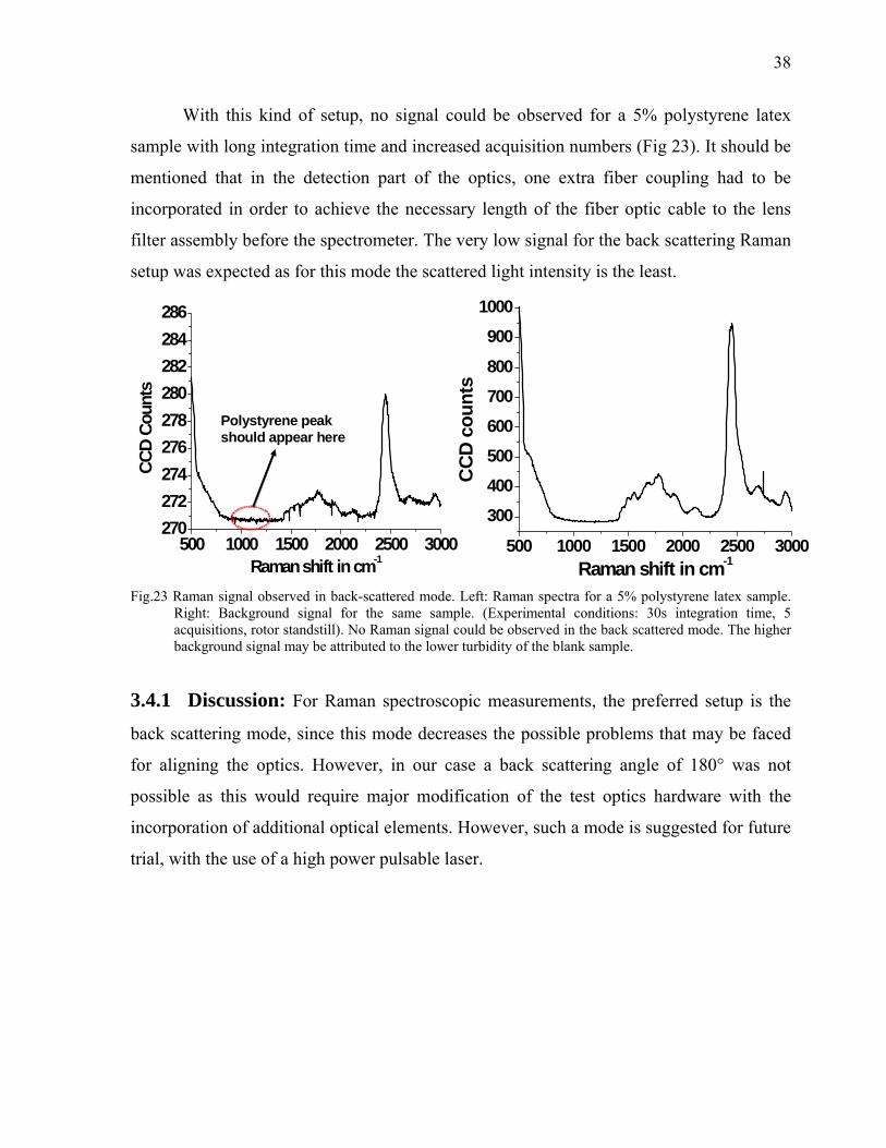
With this kind of setup, no signal could be observed for a 5% polystyrene latex
sample with long integration time and increased acquisition numbers (Fig 23). It should be
mentioned that in the detection part of the optics, one extra fiber coupling had to be
incorporated in order to achieve the necessary length of the fiber optic cable to the lens
filter assembly before the spectrometer. The very low signal for the back scattering Raman
setup was expected as for this mode the scattered light intensity is the least.
500 1000 1500 2000 2500 3000
300400500600700800
9001000
CCD
cou
nts
Raman shift in cm-1500 1000 1500 2000 2500 3000
270272274276278280282284286
CCD
Coun
ts
Raman shift in cm-1
Polystyrene peak should appear here
Fig.23 Raman signal observed in back-scattered mode. Left: Raman spectra for a 5% polystyrene latex sample.
Right: Background signal for the same sample. (Experimental conditions: 30s integration time, 5 acquisitions, rotor standstill). No Raman signal could be observed in the back scattered mode. The higher background signal may be attributed to the lower turbidity of the blank sample.
3.4.1 Discussion: For Raman spectroscopic measurements, the preferred setup is the
back scattering mode, since this mode decreases the possible problems that may be faced
for aligning the optics. However, in our case a back scattering angle of 180° was not
possible as this would require major modification of the test optics hardware with the
incorporation of additional optical elements. However, such a mode is suggested for future
trial, with the use of a high power pulsable laser.

39
Chapter 4 Small Angle Laser Light Scattering Detector for the
Analytical Ultracentrifuge
It is well established that the intensity of scattered light is dependent on the
molecular weight or the particle size. AUC experiments can also be used to measure these
two parameters. With a light scattering detector, one can measure the online molar mass
distribution of an ideal sample. AUC measurements have the advantage that, with respect
to interference from dust particles and aggregates, which typically cause problems in
traditional LS measurements a sample in the ultracentrifuge will be ideal due to the
simultaneous fractionation in the centrifugal field. Moreover, with the use of the Svedberg
equation, the sedimentation coefficient and molar mass distribution can yield the diffusion
coefficient distribution. The relationship (molar mass) ∝ (particle size)3 is the basis for
determination of particle size distribution as a function of molar mass. Since scattered light
intensity is proportional to the sixth power of particle size, detection of large aggregates
would be possible even at very low concentration. The present technique requires very
careful and time consuming measurements. As for determination of large aggregates one
needs to perform AUC experiments in a special way such that data collection is possible.
For studying biomacromolecules, light scattering experiments have proved to be quite
informative127. Light scattering studies can cover a wide variety of samples and can serve
as a general detection system128 while simultaneously supplying additional information. In
this chapter a summary of the development of a light scattering detector for AUC is
presented. A part of this work was carried out with Carlo Sarnthein, former PhD student in
our group (up to section 4.2.1)
4.1 The Initial measurement In the first step for developing a static light scattering detector for AUC, one needs
analyze the light scattering signal from an AUC cell, to determine the effect of cell
component on the signal. To study this effect experiments were performed on an optical
bench with a setup as shown in Fig. 24.
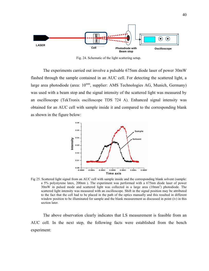
40
Fig. 24. Schematic of the light scattering setup.
The experiments carried out involve a pulsable 675nm diode laser of power 30mW
flashed through the sample contained in an AUC cell. For detecting the scattered light, a
large area photodiode (area: 10mm, supplier: AMS Technologies AG, Munich, Germany)
was used with a beam stop and the signal intensity of the scattered light was measured by
an oscilloscope (TekTronix oscilloscope TDS 724 A). Enhanced signal intensity was
obtained for an AUC cell with sample inside it and compared to the corresponding blank
as shown in the figure below:
Time axis
Inte
nsity Solvent
Sample
Fig 25. Scattered light signal from an AUC cell with sample inside and the corresponding blank solvent (sample:
a 5% polystyrene latex, 200nm ). The experiment was performed with a 675nm diode laser of power 30mW in pulsed mode and scattered light was collected in a large area (10mm2) photodiode. The scattered light intensity was measured with an oscilloscope. Shift in the signal position may be attributed to the fact that the cell had to be placed in the path of the optics manually and this resulted in different window position to be illuminated for sample and the blank measurement as discussed in point (iv) in this section later.
The above observation clearly indicates that LS measurement is feasible from an
AUC cell. In the next step, the following facts were established from the bench
experiment:
LASER Cell Photodiode with
Beam stop Oscilloscope

41
i) For a meaningful measurement of scattered light from an AUC cell, the
restricted angle of measurement is restricted to the range of 2° to 5°: This was
established by replacing the photodiode with an optical power meter and varying the
position of the power meter along the vertical direction (Fig. 26). Observation for
increased power was noted with the variation of the position of the power meter.
This can be explained by the fact that as the sample reside inside a sector-shape
sample cell, the scattered light can not emerge in all directions. The angle 0-2° can
not be reached as the corresponding area in the photosensor is the area for the
primary beam (the beam stop) since the detector to sample distance can not be
altered.
Fig.26 Experiment to establish the minimum and maximum angle of the scattered light from an AUC cell.
ii) The interference from aggregates is unavoidable in the bench measurements:
This was observed from the fact that increased intensity of light was observed from
an AUC cell with polystyrene latex sample. The signal intensity which disappeared
once the same sample was placed in the optics path after brief centrifugation.
iii) Very high background signal due to cell components: For every experimental
observation, the scattered light signal was always accompanied by a huge
background signal. A detailed observation of the primary beam at the position of the
beam stop showed that the main contribution to this signal was from the sector
shaped wall of the cell. As the light propagates through the cell sector, it touches the
sector wall and generates the background signal. Also, the cell wall gives rise to a
multiple reflection signal.
iv) Scattered light intensity for blank and the sample should be carried out from
the same cell with intact cell window position: The molar mass of samples was

42
measured from the scattered light intensity. However, the application of the Zimm
formalism resulted in non reproducible and negative molar masses. Alternately, the
calculation for molar mass was tried with the application of the following equation:
I/Io = kC wM (15)
where, I and Io are the scattered and incident light intensity and the new constant k =
(r2N/VK). This equation was derived from the equation
Rθ=Ir2/IoV=KC wM (16) The comparison for the molar mass calculations was performed with the molar mass
calculation derived from a sphere volume calculation on the basis of density data
according to the following equation:
M = mNA = NAV ρ = NA(4/3πr3) ρp (17)
Where, m is the mass of one molecule of the analyte, V is the volume occupied by it,
r is the size of the latex in radius term and ρp is the particle density. For applying this
equation, the value of ‘k’ needed to be estimated for every setup (the beam path, cell
and the solvent had to be unchanged). It was also observed that by application of this
equation, the molar mass calculation was not reproducible if the measurement for
the reference solvent intensity is performed using a different cell. Thus for carrying
out the measurement, the scattered light intensity for sample and solvent needs to be
measured from the same cell. Recording of the scattered light intensity of the sample
was done by placing the AUC cell in the optics path. The sample was then
sedimented by centrifuging for a time long enough and the scattered light intensity
for the reference solvent was recorded. For calculation of the intensities of blank and
sample, the data points at the top of the signal were averaged and regarded as the
intensity value for that signal. The following result could be obtained for one
polystyrene latex sample:
Molar mass calculated with scattered light intensity: 2.3 ×10⁹ gm/mol
Molar mass calculated from density data : 2.9×10⁹ gm/mol
In this test setup, the agreement was reasonable.

43
4.2 Online Measurement in the Centrifuge It was decided to make the online measurement of molar mass for a sedimenting
sample in the AUC with adaptation of the above mentioned setup to it. The interference
optics path in the XL centrifuge could be used for such experiments to be carried out. The
applied setup is shown in Fig. 27. Laser
Photodiode
Reflecting component from XL-I opticsBeam stop
Oscilloscope
Fig. 27. Light scattering setup for online measurement of scattered light
However, the calculated molar mass did not correspond to the reference value (the label
value of the sample). Owing to the very irregular shape of the signal from the scattered
light and its very high dissimilarity from an ideal signal shape, such a setup could possibly
always lead to an error while selecting the initial and final position of the signal for
averaging the data points. It was quite obvious that for such a setup, the ideal signal shape
should be a rectangular one. The signal should show its sharp rise when the rotor hole with
the sample cell is in front of the laser and this intensity should continue until the sector is
in the path of the optics (Fig.28). At position 1 as described in this figure, the cell sector is
not in the path, and, no light reaches the photodiode. At position 2 the edge of the cell
sector comes in the optics path and light hits the photodiode, giving signal intensity. At
position 3, the cell sector is fully in the path and observation of signal intensity continues.
At position 4, the opposite end of the cell sector comes in the path and the signal intensity
is observed. At position 5, the cell sector leaves the path, no light enters the photodiode
and no intensity is observed. With a pulsed laser synchronized with the rotor movement,
the possibility of touching the edge of the cell sector is minimized and therefore, a

44
rectangular signal can be expected. Thus, it was decided to work on improving the signal
shape as this will help to select the position in the signal for calculating the respective
intensity. Rotor movement
1 2 3 4 5
Time
Inte
nsity
Ideal signal shape
Fig.28. Description of the generation of the ideal signal shape. The red line indicates the laser beam propagation
direction. The black spot with a circle is the beam photodiode with beam stop. The trapezium shape is the representative shape of the cell sector. Inset: the desired signal shape for the scattered light intensity with the cell sector as the sample holder.
4.2.1 Signal shape improvement For measuring the scattered light intensity the XL-I optical path was used. The
complex optical components can potentially contribute to the inferior signal shape, as the
possibility that distortion occurs when passing through these optics components can not be
ruled out. As a trial, signal shape was tested with systematic removal of the “complex”
optical components. The figures 29-30 show respectively, a schematic of these
components and photograph of the setup.
Fig.29 The part in the interference optics system with the photodiode fitted into it. The glass plate , mirror and
the condenser lens were removed from the optics path for getting the ideal signal shape. (ref. fig.5 for the complete optics)

45
Photodiode
Glass plate
Fig.30 Photographs showing the fitting of the photodiode with the beam stop fitted to the optics. The photodiode
with the beam stop was fitted in the optics path by gluing it on a glass plate and by removal of the components starting from the prism in XL-I optics(ref. fig. 5)
The results of the trial, presented in Fig. 31 show that the ideal shape could be obtained
with removal of the optics components.
-3.0x10⁻⁴-2.0x10⁻⁴-1.0x10⁻⁴ 0.0 1.0x10⁻⁴ 2.0x10⁻⁴ 3.0x10-40.3
0.4
0.5
0.6
0.7
0.8
0.9
1.0
1.1
1.2
Inte
nsity
Arbotrary time scale
Removal of the glass plate in front of the Photodiode
-0.002 0.000 0.002 0.004 0.006 0.008-1
0
1
2
3
4
5
Inte
nsity
Arbitrary time scale
Removal of thePrism and other optical parts ofthe normal optics
0.0 2.0x10⁻⁵ 4.0x10⁻⁵ 6.0x10⁻⁵ 8.0x10⁻⁵ 1.0x10-40.00
0.01
0.02
0.03
0.04
0.05
0.06
0.07
0.08
0.09
Inte
nsity
Arbitrary time scale
-2.0x10⁻⁵ 0.0 2.0x10⁻⁵ 4.0x10⁻⁵ 6.0x10⁻⁵ 8.0x10⁻⁵ 1.0x10-40.00
0.02
0.04
0.06
0.08
0.10
Inte
nsity
Arbitrary time scale
Removal Camera Lens
-2.0x10⁻⁵ 0.0 2.0x10-54.0x10-56.0x10-58.0x10-51.0x10-40.00
0.01
0.02
0.03
0.04
0.05
0.06
0.07
0.08
0.09
Inte
nsity
Arbitrary time scale
Pulsed LASERTime
Inte
nsity
Ideal signal shape
Fig 31. Improvement of signal shape by simplifying the XL-I optics
Thus, with the above results, it was decided to work with the following optics setup (Fig.
32) with simplified optics for recording the scattered light intensity.
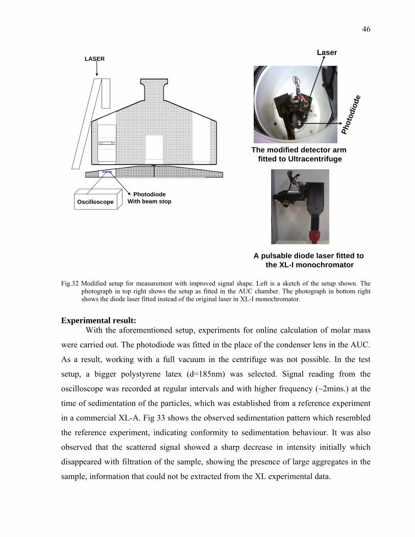
46
LASER
PhotodiodeWith beam stopOscilloscope
Laser
Phot
odio
de
The modified detector arm fitted to Ultracentrifuge
A pulsable diode laser fitted tothe XL-I monochromator
Fig.32 Modified setup for measurement with improved signal shape. Left is a sketch of the setup shown. The
photograph in top right shows the setup as fitted in the AUC chamber. The photograph in bottom right shows the diode laser fitted instead of the original laser in XL-I monochromator.
Experimental result: With the aforementioned setup, experiments for online calculation of molar mass
were carried out. The photodiode was fitted in the place of the condenser lens in the AUC.
As a result, working with a full vacuum in the centrifuge was not possible. In the test
setup, a bigger polystyrene latex (d=185nm) was selected. Signal reading from the
oscilloscope was recorded at regular intervals and with higher frequency (~2mins.) at the
time of sedimentation of the particles, which was established from a reference experiment
in a commercial XL-A. Fig 33 shows the observed sedimentation pattern which resembled
the reference experiment, indicating conformity to sedimentation behaviour. It was also
observed that the scattered signal showed a sharp decrease in intensity initially which
disappeared with filtration of the sample, showing the presence of large aggregates in the
sample, information that could not be extracted from the XL experimental data.
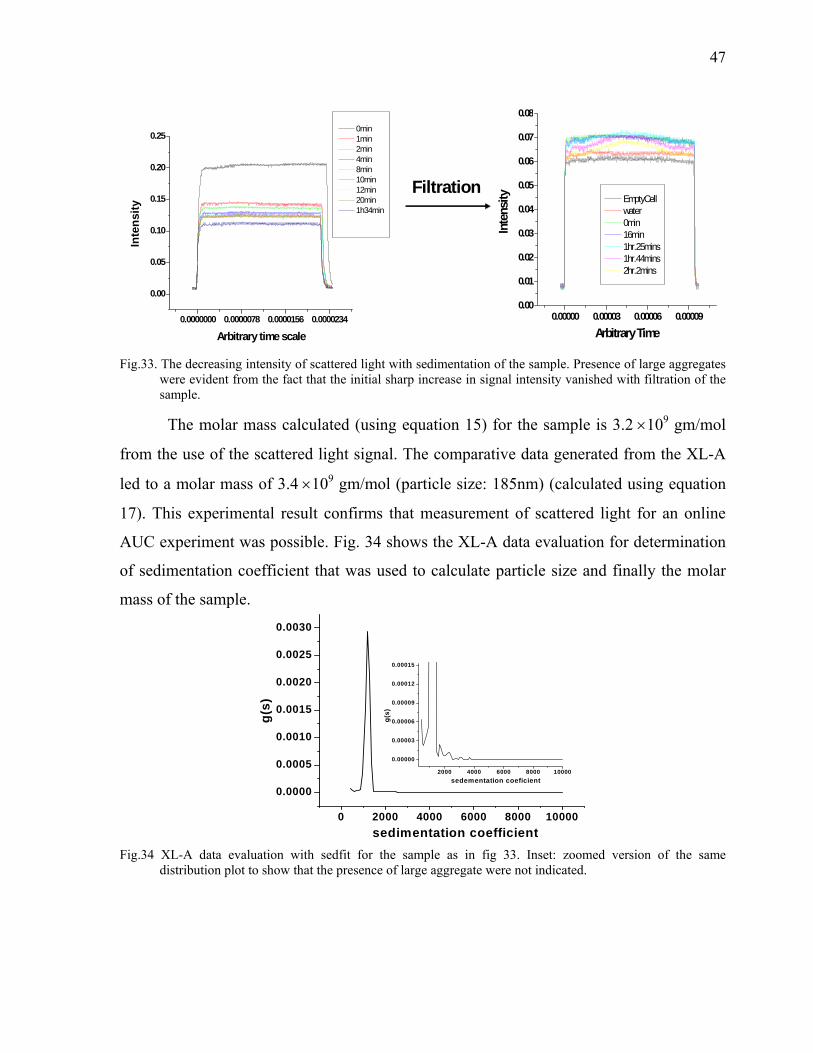
47
Fig.33. The decreasing intensity of scattered light with sedimentation of the sample. Presence of large aggregates
were evident from the fact that the initial sharp increase in signal intensity vanished with filtration of the sample.
The molar mass calculated (using equation 15) for the sample is 3.2 ×10⁹ gm/mol
from the use of the scattered light signal. The comparative data generated from the XL-A
led to a molar mass of 3.4 ×10⁹ gm/mol (particle size: 185nm) (calculated using equation
17). This experimental result confirms that measurement of scattered light for an online
AUC experiment was possible. Fig. 34 shows the XL-A data evaluation for determination
of sedimentation coefficient that was used to calculate particle size and finally the molar
mass of the sample.
0 2000 4000 6000 8000 10000
0.0000
0.0005
0.0010
0.0015
0.0020
0.0025
0.0030
g(s)
sedimentation coefficient
2000 4000 6000 8000 10000
0.00000
0.00003
0.00006
0.00009
0.00012
0.00015
g(s)
sedementation coeficient
Fig.34 XL-A data evaluation with sedfit for the sample as in fig 33. Inset: zoomed version of the same
distribution plot to show that the presence of large aggregate were not indicated.
0.00000 0.00003 0.00006 0.000090.00
0.01
0.02
0.03
0.04
0.05
0.06
0.07
0.08
Inte
nsity
Arbitrary Time
EmptyCell water 0min 16min 1hr.25mins 1hr.44mins 2hr.2mins
Filtration
0.0000000 0.0000078 0.0000156 0.0000234
0.00
0.05
0.10
0.15
0.20
0.25In
tens
ity
Arbitrary time scale
0min 1min 2min 4min 8min 10min 12min 20min 1h34min
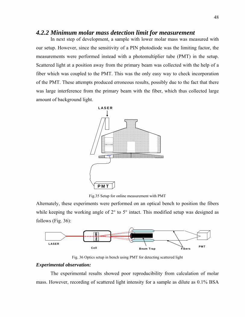
48
4.2.2 Minimum molar mass detection limit for measurement In next step of development, a sample with lower molar mass was measured with
our setup. However, since the sensitivity of a PIN photodiode was the limiting factor, the
measurements were performed instead with a photomultiplier tube (PMT) in the setup.
Scattered light at a position away from the primary beam was collected with the help of a
fiber which was coupled to the PMT. This was the only easy way to check incorporation
of the PMT. These attempts produced erroneous results, possibly due to the fact that there
was large interference from the primary beam with the fiber, which thus collected large
amount of background light. L A S E R
P M T Fig.35 Setup for online measurement with PMT
Alternately, these experiments were performed on an optical bench to position the fibers
while keeping the working angle of 2° to 5° intact. This modified setup was designed as
follows (Fig. 36):
LASERCell PM T
FibersBeam Trap Fig. 36 Optics setup in bench using PMT for detecting scattered light
Experimental observation:
The experimental results showed poor reproducibility from calculation of molar
mass. However, recording of scattered light intensity for a sample as dilute as 0.1% BSA

49
can nevertheless be observed. The molar mass calculation showed a dependency on the
selection of the calibration standard for use in equation (15). The following data were
obtained using the above mentioned setup with the use of different calibration standard for
calculation of ‘k’ in equation (15).
0 2 4 6 8 1 0 1 21 .5
2 .0
2 .5
3 .0
3 .5
4 .0
4 .5
5 .0
5 .5
6 .0 L ite ra tu re P lo t
C a lib ra t io n S ta n d a rd : 0 .1 % B S A
C a lib ra t io n S ta n d a rd : 0 .5 % B S A 1/
Mw
×10-5
C o n c e n tra tio n in m g /m l
C a lib ra t io n s tn a d a rd : 1 % B S A
Fig. 37 Plots showing the calculation of molar mass from scattered light intensity, that indicate the dependency of
experimental data on selection of the calibration standard for equation (15)
These data show the setup used cannot be correct due to the high dependency on
the calibration standard and the slope of the curves being different. An explanation for
such a variation can be the irregular background signal with respect to the fiber optics-
based scattered light collection. In the earlier setup a photodiode was used for scattered
light collection, providing a large area for the detection covering the majority of the
illuminated part of the cell sector with respect to the laser, resulting in a constant
background signal at the photodiode. This is unlikely to be possible with the use of optical
fiber. When manually placing the cell into the path of the optics, the same position can-not
be reached as high sensitivity of the PMT will produce a different background signal.
Thus, use of a larger area detector is suggested for the future. An alternate test with the use
of a biconvex lens, with a beam stop to collect the scattered light, focused on the optical
fiber (as in the setup for above experiments) was also carried out (ref. Fig. 38 below).
LASER
PM T
Biconvex lens w ith beam stop Optical fiber
Fig.38 Optics setup with the use of a biconvex lens with beam stop for collection of scattered light
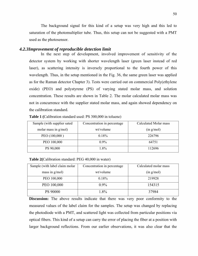
50
The background signal for this kind of a setup was very high and this led to
saturation of the photomultiplier tube. Thus, this setup can not be suggested with a PMT
used as the photosensor.
4.2.3Improvement of reproducible detection limit In the next step of development, involved improvement of sensitivity of the
detector system by working with shorter wavelength laser (green laser instead of red
laser), as scattering intensity is inversely proportional to the fourth power of this
wavelength. Thus, in the setup mentioned in the Fig. 36, the same green laser was applied
as for the Raman detector Chapter 3). Tests were carried out on commercial Poly(ethylene
oxide) (PEO) and polystyrene (PS) of varying stated molar mass, and solution
concentration. These results are shown in Table 2. The molar calculated molar mass was
not in concurrence with the supplier stated molar mass, and again showed dependency on
the calibration standard.
Table 1 (Calibration standard used: PS 300,000 in toluene)
Sample (with supplier sated
molar mass in g/mol)
Concentration in percentage
wt/volume
Calculated Molar mass
(in g/mol)
PEO (100,000 ) 0.18% 226796
PEO 100,000 0.9% 64751
PS 90,000 1.8% 112696
Table 2(Calibration standard: PEG 40,000 in water)
Sample (with label claim molar
mass in g/mol)
Concentration in percentage
wt/volume
Calculated molar mass
(in g/mol)
PEO 100,000 0.18% 219928
PEO 100,000 0.9% 154315
PS 90000 1.8% 37984
Discussion: The above results indicate that there was very poor conformity to the
measured values of the label claim for the samples. The setup was changed by replacing
the photodiode with a PMT, and scattered light was collected from particular positions via
optical fibers. This kind of a setup can carry the error of placing the fiber at a position with
larger background reflections. From our earlier observations, it was also clear that the
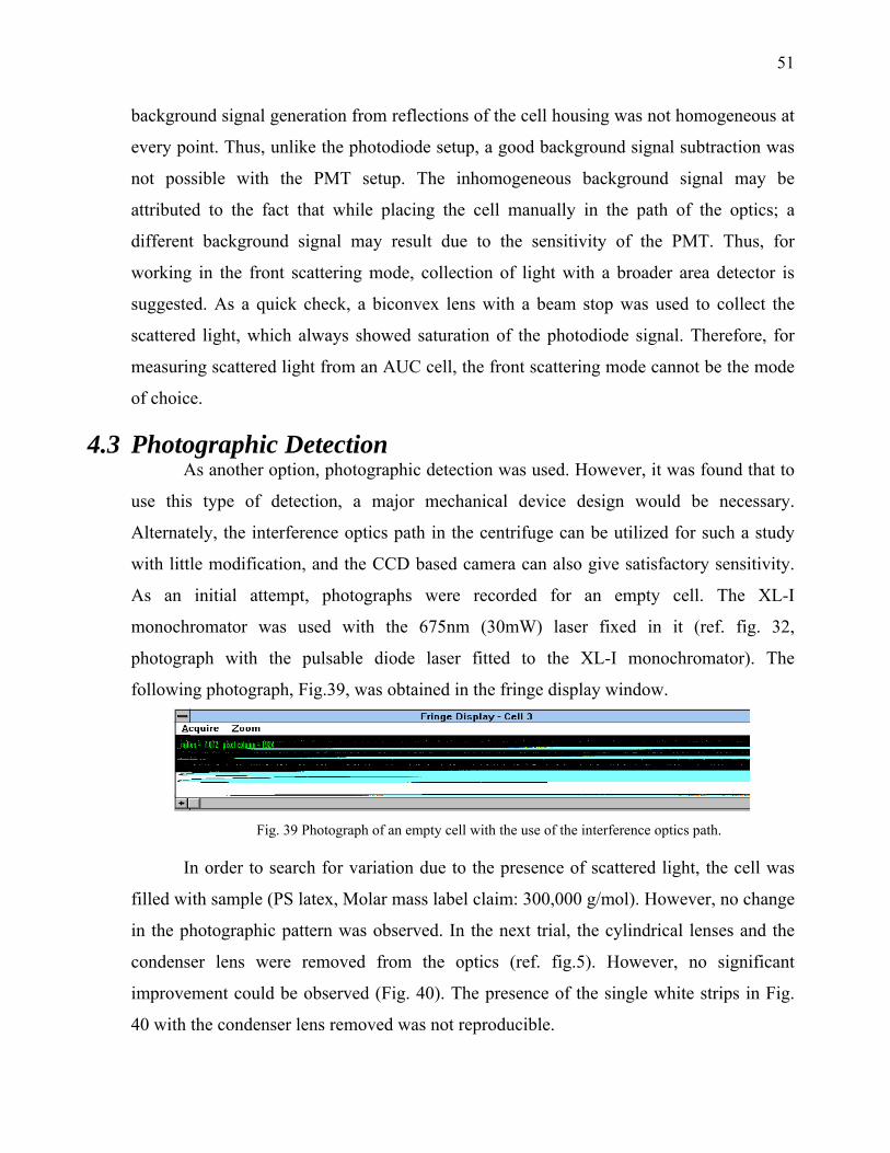
51
background signal generation from reflections of the cell housing was not homogeneous at
every point. Thus, unlike the photodiode setup, a good background signal subtraction was
not possible with the PMT setup. The inhomogeneous background signal may be
attributed to the fact that while placing the cell manually in the path of the optics; a
different background signal may result due to the sensitivity of the PMT. Thus, for
working in the front scattering mode, collection of light with a broader area detector is
suggested. As a quick check, a biconvex lens with a beam stop was used to collect the
scattered light, which always showed saturation of the photodiode signal. Therefore, for
measuring scattered light from an AUC cell, the front scattering mode cannot be the mode
of choice.
4.3 Photographic Detection As another option, photographic detection was used. However, it was found that to
use this type of detection, a major mechanical device design would be necessary.
Alternately, the interference optics path in the centrifuge can be utilized for such a study
with little modification, and the CCD based camera can also give satisfactory sensitivity.
As an initial attempt, photographs were recorded for an empty cell. The XL-I
monochromator was used with the 675nm (30mW) laser fixed in it (ref. fig. 32,
photograph with the pulsable diode laser fitted to the XL-I monochromator). The
following photograph, Fig.39, was obtained in the fringe display window.
Fig. 39 Photograph of an empty cell with the use of the interference optics path.
In order to search for variation due to the presence of scattered light, the cell was
filled with sample (PS latex, Molar mass label claim: 300,000 g/mol). However, no change
in the photographic pattern was observed. In the next trial, the cylindrical lenses and the
condenser lens were removed from the optics (ref. fig.5). However, no significant
improvement could be observed (Fig. 40). The presence of the single white strips in Fig.
40 with the condenser lens removed was not reproducible.
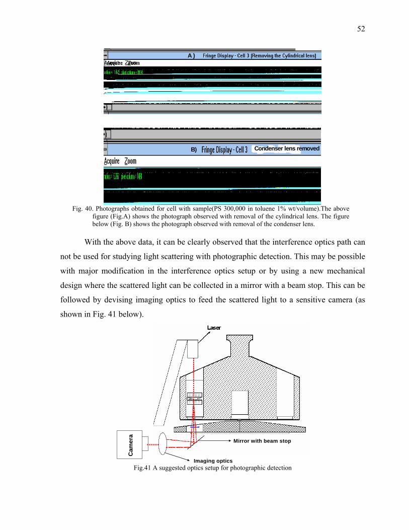
52
A )
B) Condenser lens removed
Fig. 40. Photographs obtained for cell with sample(PS 300,000 in toluene 1% wt/volume).The above
figure (Fig.A) shows the photograph observed with removal of the cylindrical lens. The figure below (Fig. B) shows the photograph observed with removal of the condenser lens.
With the above data, it can be clearly observed that the interference optics path can
not be used for studying light scattering with photographic detection. This may be possible
with major modification in the interference optics setup or by using a new mechanical
design where the scattered light can be collected in a mirror with a beam stop. This can be
followed by devising imaging optics to feed the scattered light to a sensitive camera (as
shown in Fig. 41 below).
Mirror with beam stop
Imaging optics
Cam
era
Fig.41 A suggested optics setup for photographic detection
53
4.4 Conclusion and Outlook The experiments performed indicate that reliable measurement of scattered light
from an AUC cell is possible. However, for such a detection system to work, it is
necessary to devise a setup with satisfactory sensitivity and reproducibility. The presence
of large background signal, currently ~80% of the total signal for photodiode
measurements, must be minimized. In future efforts for a functional small angle light
scattering detector, the following points are suggested.
i) Use of a laser with better beam profile: This can contribute to a reduced reducing
background signal. In the above mentioned experiments, a diode laser was used, which
has an elliptical beam shape and significant stray light. For a better beam profile one
may choose a gas laser. The use of a space filter in the incident beam path could also
sufficiently reduce the stray light which in turn will reduce the reflections from the cell
sector window.
ii) Use of larger area detector: It was observed in the above experiments that the
reflections from the cell sector are not the same in all directions. Thus, it is necessary
to average the background intensity of the light from the primary beam. This can be
achieved by the use of a larger area diode. Since more sensitivity is also highly desired,
commercially available Avalanche photodiodes (APD) can be used. This was was by
placing the APD in a housing so that it can be exchanged with the condenser lens in
interference optics. However, the construction of an adaptable circuit to the AUC could
not be completed.
iii) Back-scattering mode: In all the above experiments, the backscattering mode was
not attempted due to the necessity of major mechanical modification to the
illumination optics. This mode would diminish the background intensity greatly, and
therefore, is suggested for future developments.

54
Chapter. 5 Fast Fiber Optics Based Multiwavelength Detector for
Analytical Ultracentrifugation
Multiple wavelength study during an ultracentrifugation experiment has proven to
be advantageous, in particular to study interacting macromolecular systems such as
proteins129-131. A multiwavelength study will generate the possibility to exploit a new
source of information: the absorption spectra of the solution at different positions in the
centrifugal field. A combination of absorption spectra, scanned at multiple radii, and radial
profiles scanned at multiple wavelengths, forms a two-dimensional data surface in radius-
wavelength-absorption space, and so contains a lot more information than single radial
profiles. The analysis consists of decomposition in terms of products of extinction profiles
and exponentials, a problem that is generally much better conditioned than fitting
exclusively. Also, the detection of the wavelength dependency of turbidity opens up the
possibility to obtain independent information on the particle size in addition to the usual
sedimentation coefficient distribution for colloidal systems132-134. In the history of AUC, it
has been clear that significant effort from many workers towards the development in the
field of UV/Vis detection system. The contribution from Flossdorf135 significantly enhance
the detected UV/Vis intensity as did the introduction of a photomultiplier detection system
in commercial Beckman instruments49. In his attempt to enhance the UV intensity
Flossdorf136 used a parabolic mirror based collimator illumination system, and cylinder
optics, to optimize the illumination band in the rotor so that only the two sectors in a cell
are illuminated. However, the demand of AUC has become higher and higher with the
advent of cheap and powerful computer based resources. This became clear with the
introduction of the commercial Beckman Optima XL-A AUC, which far exceeds the
experimental possibilities a few decades ago, resulting in increasing demands for data
quality and accuracy. Despite this, development in the field of data evaluation has
remained much faster than the development in the optical detection systems.

55
Application for a Multiwavelength detector include determination of extinction
coefficients137 for complicated mixtures, and sedimentation velocity12 and sedimentation
equilibrium138 experiments for biopolymers, although in the later two cases results
reported were for only three scanning wavelengths in the XL-I AUC. However, they
illustrate the potential of working simultaneously with hundreds of wavelengths, allowing
the user to generate a wavelength scan to every radial position thereby discriminating
solutes in a more practical way to visualize. One can foresee the information available
from such an experiment for an interacting, complex polymeric mixture. Also the
wavelength dependence of the turbidity of colloidal samples is useful to detect as this
contains information about their particle size according to the MIE scattering theory139-142.
With the advent of global analysis approaches for AUC data, Multiwavelength analysis
will become an especially important technique for all light-absorbing samples of a
colloidal or polymeric nature. With the possibility of fast data collection, another
dimension can be added to AUC experiments as speed profile experiments become
possible, whereby data is collected simultaneously during acceleration of the centrifuge
from 0-60000 rpm. If the detector can collect data with a data acquisition rate on the order
of ms, a sedimentation velocity experiment can be designed that with the centrifuge being
accelerated from 0-60000 rpm, experimental data can be collected with a minimal
diffusion broadening. Parallel to the development of these AUC methodologies, there has
also been advances in the UV/Vis technology. Modern UV/Vis spectrometers use CCD
line arrays for simultaneous detection of a large number of wavelengths, which is
essentially only limited by the CCD array pixel number as well as the quality of the
applied diffraction grating for the dispersion of the incoming white light. These
spectrometers not only do allow for simultaneous detection of the entire UV-Vis
wavelength range, they are furthermore very fast and cheap. Commonly available
spectrometers like the USB2000 by Ocean Optics allow for scanning times of down to 3
ms for an entire UV-Vis spectrum 143. More recent instruments like the Ocean Optics
HR4000144 or the series of CCD and ICCD based spectrometers available from LOT-
Oriel145 are orders of magnitude faster and can scan UV-Vis spectra as fast as 10 µs. The
cooled spectrometers give a quite broad linear dynamic range with the advantage of
56
working with low dark current due to cooling145. However, although these fast and
powerful UV-Vis detectors are available, they have not yet been applied as detectors for
AUC’s. One of the reasons could be that these spectrometers are based on fiber optics and
also operate with incoming white light. White light with wavelength-dependent refractive
indices makes the precise use of refractive optics impossible, at least in the UV range
where the conventional achromatic lenses cannot be applied, and the same is true in the
visible range if an expensive UV achromat lens system is applied. This obstacle has no
parallel in previous AUC optics, that always operates with monochromatic light – or in
case of the XL-A AUC with a torroidally curved diffraction grating producing
monochromatic light. It is only for this reason that the challenge of a Multiwavelength
AUC optics has not previously been undertaken despite the potential benefits. Thus with
this motivation, it was decided to start the effort to construct a multiwavelength detector
for AUC. The work was carried out in collaboration with the Polymer Physics department
of BASF-AG, Ludwigshafen, Germany.
This work was carried on the basis of previous development and experiences of a
former PhD student in our group, Patrycia Maciejewska. The work will be divided into
generation: The first generation comprises implementation of the previous work with
removal problems that were associated with it. The second generation describes
development for the data evaluation software and use of partial mirror based optics. In the
third generation attempt will be made to design optics and instrument hardware with
removal of experienced errors and instrument problem (heat sink modification from
preparative to XL-I).
5.1 Development of a Fast Fiber Optics-based Multiwavelength detector for AUC (Generation 1)
5.1.1 The work so far Work for developing a fast fiber optics-based Multiwavelength VU/Vis detector
was in progress. The following conclusions were drawn from the previous work:

57
i) Construction of a Multiwavelength UV/Vis detector on an preparative XL
Ultracentrifuge platform is possible, that can generate Multiwavelength UV/Vis
range data.
ii) Reduction of the scan time by a factor > 100 is possible over XL-A, at
comparable data quality in time scan mode, however radial scan mode so far
remains as slow as XL-A.
iii) Two operation modes could be achieved: Constant velocity – radial scanning
and time mode scan – time scanning at constant radius and movement of
detector towards meniscus for fast detection could be achieved.
The following problems were highlighted from the initial experience from this work:
i) Very low light intensity through the optics. The loss of light intensity was
especially severe in the UV region with almost no intensity at wavelengths
below 300nm. Fiber bending also contributes to the loss of intensity.
ii) Lower than expected data quality.
5.1.2 Bench observations to optimize light intensity Careful observation was performed for the alignment of each optical component
used in the experimental setup. A scheme of the previous optical setup is shown in Fig. 82
below:
Fig.42 Experimental optics setup used by the previous worker. 1-600 micron patch fiber, UV-Vis (Ocean Optics).
2- The collimating lens system (self built) f = 20.6 mm biconvex. 3-90 °Quartz prism. 4-Slit-lens assembly (from the XL-A) only one lens f = 10 mm biconvex. 5- Focuser (OZ Optics) two lenses f = 10 & 15 mm. 6-1000 micron patch fiber, UV-Vis (Ocean Optics).

58
A simulation of the setup was constructed on an optical bench using microbench
mechanical components from Linos, Göttingen, Germany. It was found that due to
inaccurate design of the mechanical housing in the setup, optimal movement of the slit
was not possible for it to be in the aligned position. The 25um slit (used from original
Beckman XL-A slit-lens assembly, position 4 in Fig. 42) was glued in a cylindrical
housing in a previously aligned position. It was decided to replace this part in the
mechanical arm with a new design as follows. The design of the detection optics was
altered to allow housing of a 20mm biconvex lens o collect transmitted light, followed by
a 25 µm precision slit (MellesGriot, Bensheim, Germany) to define the spatial resolution
and a 10mm biconvex lens to focuss of light emerging from precision slit back to the fiber.
The schematic of this new setup is shown in the Fig.43.
67
Fig. 43. Modified detector arm. The detector arm. 1, 2 and 3 are same as in the earlier setup. (4) Biconves lens f =
20mm (5) Slit of dimension 25 µm, (6) Biconvex lens f =10mm (7) 600µm patch fiber (Ocean optics). The light path is also shown schematically.
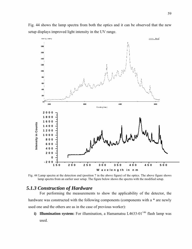
59
Fig. 44 shows the lamp spectra from both the optics and it can be observed that the new
setup displays improved light intensity in the UV range.
1 5 0 2 0 0 2 5 0 3 0 0 3 5 0 4 0 0 4 5 0 5 0 0- 2 0 0
02 0 04 0 06 0 08 0 0
1 0 0 01 2 0 01 4 0 01 6 0 01 8 0 02 0 0 0
Inte
nsity
in C
ount
s
W a v e l e n g t h i n n m
Fig. 44 Lamp spectra at the detection end (position 7 in the above figure) of the optics. The above figure shows lamp spectra from an earlier user setup. The figure below shows the spectra with the modified setup.
5.1.3 Construction of Hardware For performing the measurements to show the applicability of the detector, the
hardware was constructed with the following components (components with a * are newly
used one and the others are as in the case of previous worker):
i) Illumination system: For illumination, a Hamamatsu L4633-01146 flash lamp was
used.

60
ii) Modified Heatsink: An XL preparative Ultracentrifuge heat sink was modified at
BASF-AG. Six holes were drawn to allow for fiber feedthroughs and electrical
feedthroughs to be fitted.
iii) Optical Fibers: 600 micron patch fiber with SMA 905 connector, UV-Vis and
1000 micron patch fiber from Oceanoptics, Duiven The Netherlands.
iv) Spectrometer: USB 2000 Fiber Optics Spectrometer (UV/Vis, SMA 905
connector), Ocean Optics BV, Duiven, the Netherlands.
v) Electrical feedthrough: 18 pin electrical feedthrough for electrical connection of
the linear actuator, from Electronik GmbH, Munich, Germany
vi) Optical Bench: From Owis GmbH, Göttingen, Germany with x, y, z and angular
adjustment for coupling the light from the flash lamp and the fiber.
vii) Optical stage: From OWIS GmbH, Staufen, Germany with fine-adjustment
screws in the x and y directions, for the precise adjustment of the detection optics
part of the detector arm.
viii) Reflection light gate: This system was developed at BASF, Ludwigshafen,
Germany. In this system, a photoelectric reflection light gate is fixed to the bottom
of the vacuum chamber which consists of a continuously light-emitting LED and a
fast photodiode. A mirror (a polished small strip at the rotor bottom) fitted on the
base of the analytical rotor reflects the light of the LED. This alignment provides a
TTL pulse for each revolution of the rotor.
ix) *Precision Slit: 25 µm precision slit from MellesGriot, Bensheim, Germany
x) *Lens Holder with x-, y- adjustment: From OWIS GmbH, Staufen, Germany.
Apart from the above mentioned components, the commercially available parts as
described in figure 43 were used. The photographs of the detector arm and the arm placed
inside the AUC chamber are shown in the Fig. 45.
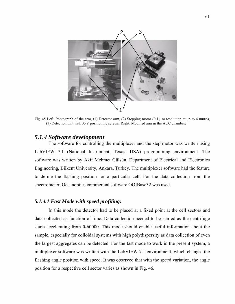
61
2
1
3
Fig. 45 Left. Photograph of the arm, (1) Detector arm, (2) Stepping motor (0.1 µm resolution at up to 4 mm/s),
(3) Detection unit with X-Y positioning screws. Right: Mounted arm in the AUC chamber.
5.1.4 Software development The software for controlling the multiplexer and the step motor was written using
LabVIEW 7.1 (National Instrument, Texas, USA) programming environment. The
software was written by Akif Mehmet Gülsün, Department of Electrical and Electronics
Engineering, Bilkent University, Ankara, Turkey. The multiplexer software had the feature
to define the flashing position for a particular cell. For the data collection from the
spectrometer, Oceanoptics commercial software OOIBase32 was used.
5.1.4.1 Fast Mode with speed profiling: In this mode the detector had to be placed at a fixed point at the cell sectors and
data collected as function of time. Data collection needed to be started as the centrifuge
starts accelerating from 0-60000. This mode should enable useful information about the
sample, especially for colloidal systems with high polydispersity as data collection of even
the largest aggregates can be detected. For the fast mode to work in the present system, a
multiplexer software was written with the LabVIEW 7.1 environment, which changes the
flashing angle position with speed. It was observed that with the speed variation, the angle
position for a respective cell sector varies as shown in Fig. 46.
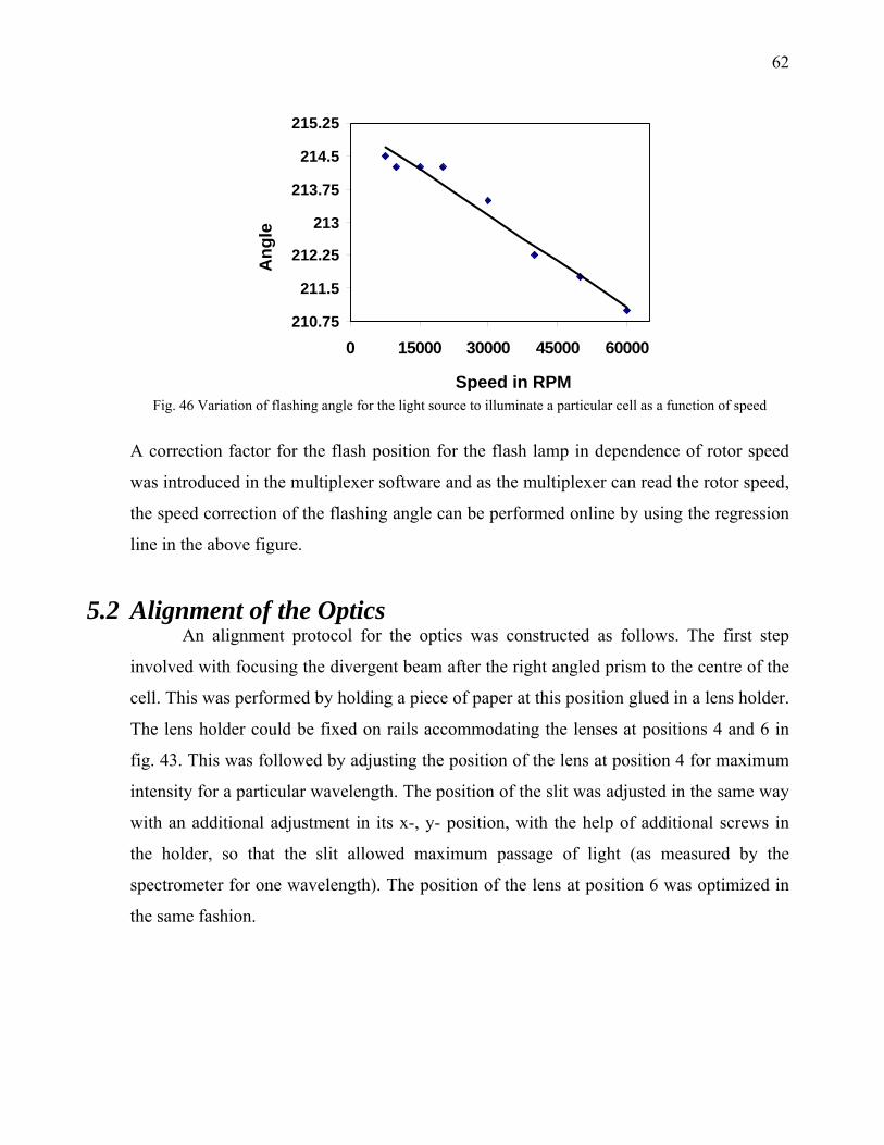
62
210.75
211.5
212.25
213
213.75
214.5
215.25
0 15000 30000 45000 60000
Speed in RPM
Ang
le
Fig. 46 Variation of flashing angle for the light source to illuminate a particular cell as a function of speed
A correction factor for the flash position for the flash lamp in dependence of rotor speed
was introduced in the multiplexer software and as the multiplexer can read the rotor speed,
the speed correction of the flashing angle can be performed online by using the regression
line in the above figure.
5.2 Alignment of the Optics An alignment protocol for the optics was constructed as follows. The first step
involved with focusing the divergent beam after the right angled prism to the centre of the
cell. This was performed by holding a piece of paper at this position glued in a lens holder.
The lens holder could be fixed on rails accommodating the lenses at positions 4 and 6 in
fig. 43. This was followed by adjusting the position of the lens at position 4 for maximum
intensity for a particular wavelength. The position of the slit was adjusted in the same way
with an additional adjustment in its x-, y- position, with the help of additional screws in
the holder, so that the slit allowed maximum passage of light (as measured by the
spectrometer for one wavelength). The position of the lens at position 6 was optimized in
the same fashion.

63
5.3 Results
5.3.1 Time Domain Data: As was realized in the previous work, this mode allows a
faster sedimentation velocity experiment to be designed with generation of huge
amount of data points. Fig. 47 shows results obtained from a BSA sample (1mg/mL
prepared in 0.1N NaCl) for this mode of operation.
Tim
e
Abs
orba
nce
W avelength in nm Fig.47 Sedimentation velocity experiment of BSA. 3D view of time mode scan (showed detection up to
240nm). Speed: 50000 rpm, detector position: 6.3cm, Data integration time: 100ms, 1 average. Sample: BSA 1mg/mL in 0.1M NaCl prepared by dilution.
0 2000 4000 6000 8000 10000 120000.0
0.2
0.4
0.6
0.8
Abso
rban
ce
Time in seconds Fig. 48 Absorbance vs time plot for BSA 1 g/L at 280nm. (Experimental conditions; Rotor speed: 50000
rpm, Slit position: 6.1 cm. Data recorded with 100ms integration time and 1 average). The data were not corrected for the reference solvent.
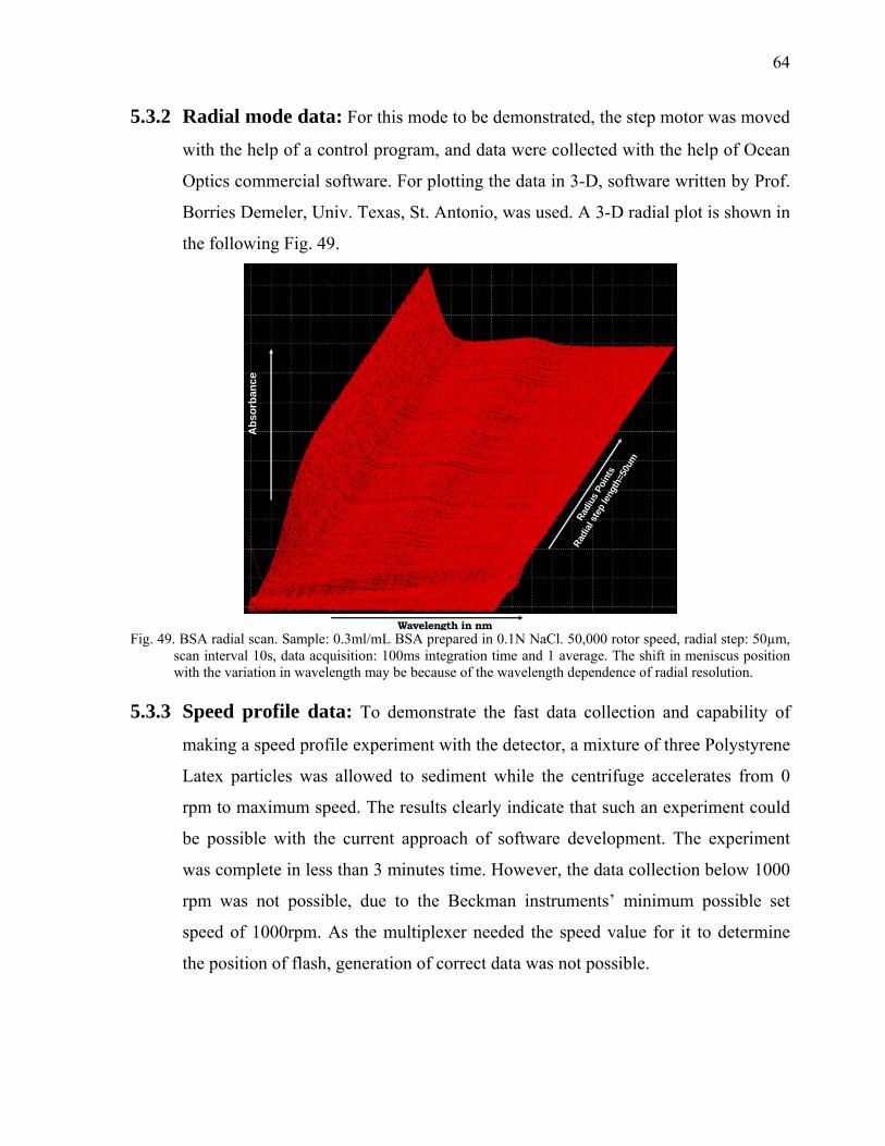
64
5.3.2 Radial mode data: For this mode to be demonstrated, the step motor was moved
with the help of a control program, and data were collected with the help of Ocean
Optics commercial software. For plotting the data in 3-D, software written by Prof.
Borries Demeler, Univ. Texas, St. Antonio, was used. A 3-D radial plot is shown in
the following Fig. 49.
Wavelength in nm
Radi
us P
oint
s
Radi
al st
ep le
ngth
=50u
m
Abs
orba
nce
Fig. 49. BSA radial scan. Sample: 0.3ml/mL BSA prepared in 0.1N NaCl. 50,000 rotor speed, radial step: 50µm,
scan interval 10s, data acquisition: 100ms integration time and 1 average. The shift in meniscus position with the variation in wavelength may be because of the wavelength dependence of radial resolution.
5.3.3 Speed profile data: To demonstrate the fast data collection and capability of
making a speed profile experiment with the detector, a mixture of three Polystyrene
Latex particles was allowed to sediment while the centrifuge accelerates from 0
rpm to maximum speed. The results clearly indicate that such an experiment could
be possible with the current approach of software development. The experiment
was complete in less than 3 minutes time. However, the data collection below 1000
rpm was not possible, due to the Beckman instruments’ minimum possible set
speed of 1000rpm. As the multiplexer needed the speed value for it to determine
the position of flash, generation of correct data was not possible.

65
0 30 60 90 120 150 180
0.00
0.01
0.02
0.03
0.04
Der
ivat
ive
Time in Seconds0 30 60 90 120 150 180
-0.2
0.0
0.2
0.4
0.6
0.8
1.0
1.2
1.4
Abso
rban
ce
Time in seconds Fig. 50. Fast sedimentation velocity experiment with a Polystyrene Latex mixture of sizes 190nm, 305nm and
605nm in 1:2:2 mixing ratio by wt.; data collected at wavelength 350nm. Left: Experimental raw data. Right: The derivative curve was generated performing differentiation after 5 point FFT smoothing. Slit position: 6.4 cm.
5.4 Discussion
With the available preliminary results, it was clear that the setup should be suitable
for constructing a Multiwavelength UV/Vis detector with a much improved data collection
speed, as compared to the existing detector with the need to use fibers as the light guide.
This setup would allow the option of “plug and play” for different components to work on
further developments. However, following problems would have to be circumvented for
such a detector:
i) Use of optical elements free of chromatic aberration: Lens based optics give rise to
the problem of wavelength dependency of radial resolution. This problem may become
severe with the use of more and more refracting components. Also, while aligning one
can only work with one wavelength for fine adjustments, which would make data
inferior for other wavelengths. Thus the error introduced in the data will depend upon
two factors: data quality limited by optics resolution and by alignment. However, it
may be mentioned that this effect is also present in the commercial Beckmann XL-
instruments’ as they use lens based scanning systems. Fig. 51 shows the wavelength
dependence of radial resolution, as observed with the present optics with that in XL-A
optic.

66
5.94 5.97 6.00 6.03 6.06 6.09 6.12 6.15 6.18-20
0
20
40
60
80
100
120
140
160In
tens
ity
Radius Position
250 nm 300nm 400 nm 450nm
400nm, 90um
450nm, 73um
300nm, 83um
250nm,80um
20 40 60 80 100
0
300
600
900
1200
1500
Wavelength: 250nmOptics resolution: 100um
Wavelength: 300nmOptics resolution: 90um
Wavelength: 450nmOptics resolution: 60um
Inte
nsity
Distance moved by the step motor in um
Wavelength: 400nmOptics resolution: 55um
XL-A Multiwavelength
Fig. 51 Optical resolution dependence on wavelength. A counterbalance cell hole was scanned with the
movement of the step motor. Experimental condition for Multiwavelength detector: step motor movement:3um/step, data acquisition:100µs integration time, 1averaging. For XL-A, intensity scan is performed on the counter balance holes as the detector scans the counter balance cell radially. As expected, the effect is more severe in case of Multiwavelength detector due to the use of larger focal length lenses.
ii) Use of Parallel light for the illumination optics: The use of parallel light for the
detection optics is highly desirable, since with a divergent optics, achieving satisfactory
alignment will be very difficult. One problem may be cited that of difficulty while fine
adjusting the optics for making coincidence of the optical axis of illumination and
detection optics. During alignment of the optics, this was achieved by moving the x, y
screws at the detection optics to the maximum intensity in the lamp spectrum for a
particular wavelength. However, it is possible that the whole light may not be entering
the collecting lens. Also, there is the problem of inefficient focusing by the outer part,
compared with the central part of the lens. Also, the use of larger diameter lenses can
not be suggested because of the space constraint, as for using a bigger diameter lens one
will have to select lenses with higher focal length and consequently a longer detector
arm as shown in Fig. 52.

67
Colle
ctio
n le
ns
(lens
at p
ositi
on 4
in fi
g.38
)
Ligh
t not
ente
ring
the c
ollec
ting
lens
Fig. 52: Inefficient collection of the transmitted light by the collection lens
iii) Design of the optics arm without fiber bending: During the measurements, we
investigated the amount of light intensity loss because of fiber bending as this is a well
known phenomenon. Also, the design of the illumination optics had a fiber bending
point of ~90°. The light loss was quite prominent (Fig. 53) in the UV range compared
to the visible range and the peak at the lowest possible wavelength (~228nm) in the
lamp spectra vanished with the detector arm transferred to the centrifuge.
150 200 250 300 35 0 400 450 500 550-500
0
500
1 000
1 500
2 000
2 500
3 000
3 500
4 000
Inte
nsity
in c
ount
s
W a ve le n g th in n m
A rm a t th eB e n c h
A rm a tC en trifu g e~ 1 0 0 0
~ 3 0 0
(w ith o u t f ib e r b e n d in g )
(w ith 9 0 ° f ib e r b e n d in g )
Fig. 53 Loss of light due to fiber bending. The detector was aligned and the lamp spectrum was recorded
at the bench (Arm at the bench). Lamp spectra recorded after the detector was transferred to the centrifuge (Arm at the centrifuge), showed about 70% light loss in the UV region.
Thus for the next generation, it was postulated to work on a design to minimize fiber
bending, using mirror based optics with maximum achievable collimation.

68
Chapter 6 Fast Fiber Optics Based Multiwavelength Detector for AUC
Generation-II
To this point it can be said empirically that a Multiwavelength detection system
can be constructed on a preparative Ultracentrifuge platform with the possibility to
generate 3-D radial scans and much faster data acquisition. A further improvement can be
made with the introduction of sophisticated software with improved optics that can
generate data that are free of optical errors. This chapter covers software development for
the detector, with possible developments and replacements of optical parts on the basis of
the first generation development.
6.1 Hardware Development It was envisaged during the first generation development that working with a
collimated light beam should allow for higher intensity in the optics, and this was
therefore used for the illumination optics. However, since collimation optics constructed
by the use of lenses will always be accompanied by the chromatic aberration error
replacing these optics with a mirror-based setup was expected to be free of this error as
mirrors do not show chromatic aberration. An off axis parabolic (OAP) mirror could serve
for such a purpose. Also an OAP can result in enhanced UV intensity136,137. Introduction of
such a system can result in quite encouraging data generation as this kind of an
illumination system will diminish the error due to alignment and chromatic aberration. A
representative sketch of the mirror setup for the illumination optics is shown in the fig 54.
Off Axis
parabolic mirror
(OAP)
Cell sector
Plan
e m
irror
F iber
Fibe
r tip
Coi
ncid
ing
with
th
e fo
cus
of th
e O
AP
Collim ated light
Fig.54 Setup for collimated white light in the illumination optics.
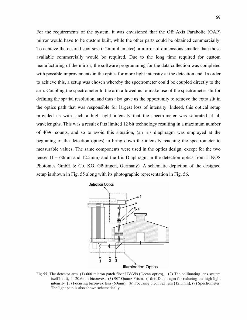
69
For the requirements of the system, it was envisioned that the Off Axis Parabolic (OAP)
mirror would have to be custom built, while the other parts could be obtained commercially.
To achieve the desired spot size (~2mm diameter), a mirror of dimensions smaller than those
available commercially would be required. Due to the long time required for custom
manufacturing of the mirror, the software programming for the data collection was completed
with possible improvements in the optics for more light intensity at the detection end. In order
to achieve this, a setup was chosen whereby the spectrometer could be coupled directly to the
arm. Coupling the spectrometer to the arm allowed us to make use of the spectrometer slit for
defining the spatial resolution, and thus also gave us the opportunity to remove the extra slit in
the optics path that was responsible for largest loss of intensity. Indeed, this optical setup
provided us with such a high light intensity that the spectrometer was saturated at all
wavelengths. This was a result of its limited 12 bit technology resulting in a maximum number
of 4096 counts, and so to avoid this situation, (an iris diaphragm was employed at the
beginning of the detection optics) to bring down the intensity reaching the spectrometer to
measurable values. The same components were used in the optics design, except for the two
lenses (f = 60mm and 12.5mm) and the Iris Diaphragm in the detection optics from LINOS
Photonics GmbH & Co. KG, Göttingen, Germany). A schematic depiction of the designed
setup is shown in Fig. 55 along with its photographic representation in Fig. 56.
Fig 55. The detector arm. (1) 600 micron patch fiber UV/Vis (Ocean optics), (2) The collimating lens system
(self built), f= 20.6mm biconvex, (3) 90° Quartz Prism, (4)Iris Diaphragm for reducing the high light intensity (5) Focusing biconvex lens (60mm), (6) Focusing biconvex lens (12.5mm), (7) Spectrometer. The light path is also shown schematically.
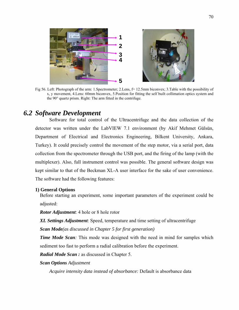
70
1234
5 Fig 56. Left: Photograph of the arm: 1.Spectrometer; 2.Lens, f= 12.5mm biconvex; 3.Table with the possibility of
x, y movement, 4.Lens: 60mm biconvex, 5.Position for fitting the self built collimation optics system and the 90° quartz prism. Right: The arm fitted in the centrifuge.
6.2 Software Development Software for total control of the Ultracentrifuge and the data collection of the
detector was written under the LabVIEW 7.1 environment (by Akif Mehmet Gülsün,
Department of Electrical and Electronics Engineering, Bilkent University, Ankara,
Turkey). It could precisely control the movement of the step motor, via a serial port, data
collection from the spectrometer through the USB port, and the firing of the lamp (with the
multiplexer). Also, full instrument control was possible. The general software design was
kept similar to that of the Beckman XL-A user interface for the sake of user convenience.
The software had the following features:
1) General Options Before starting an experiment, some important parameters of the experiment could be
adjusted:
Rotor Adjustment: 4 hole or 8 hole rotor
XL Settings Adjustment: Speed, temperature and time setting of ultracentrifuge
Scan Mode(as discussed in Chapter 5 for first generation)
Time Mode Scan: This mode was designed with the need in mind for samples which
sediment too fast to perform a radial calibration before the experiment.
Radial Mode Scan : as discussed in Chapter 5.
Scan Options Adjustment
Acquire intensity data instead of absorbance: Default is absorbance data

71
Filter scan intensities below a certain level: Only in radial mode scan
Stop XL after last scan
Make radial calibration after experiment
Method Scan Options Adjustment
Delayed Start: Time delay before the first scan
Time between Scans: In Radial Mode only
Number of Scans: In Radial Mode only
Experiment Directory: To define data saving path.
2) Cell Options
For both, time mode and radial mode scans, after enabling desired cells, their experimental
parameters should be adjusted, which differ in the two modes
Common Options
Here one can select up to four wavelengths for online radial scan observations, also
these radial scans are saved in separate files. The feature of saving the full spectra
with the selected wavelength range is implemented.
Time Mode Options
Radius: Detector position in the cell
Acquisition/Averaging time for one data point
Radial Mode Options
Rmin and Rmax: minimum and maximum radial distance
Radial Step: radial step size between two detector readings (settings possible from
0.1- 100 micrometer)
Replicates: number of data points collected at each wavelength
Set All Settings Identical to Cell 1: set the parameters of cell 1 for each cell
The operational front panel of the software is shown in Fig. 57.
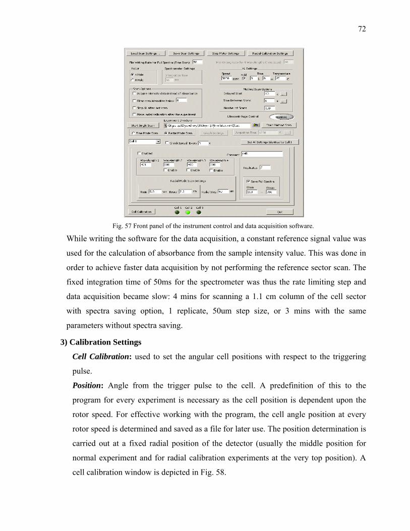
72
Fig. 57 Front panel of the instrument control and data acquisition software.
While writing the software for the data acquisition, a constant reference signal value was
used for the calculation of absorbance from the sample intensity value. This was done in
order to achieve faster data acquisition by not performing the reference sector scan. The
fixed integration time of 50ms for the spectrometer was thus the rate limiting step and
data acquisition became slow: 4 mins for scanning a 1.1 cm column of the cell sector
with spectra saving option, 1 replicate, 50um step size, or 3 mins with the same
parameters without spectra saving.
3) Calibration Settings
Cell Calibration: used to set the angular cell positions with respect to the triggering
pulse.
Position: Angle from the trigger pulse to the cell. A predefinition of this to the
program for every experiment is necessary as the cell position is dependent upon the
rotor speed. For effective working with the program, the cell angle position at every
rotor speed is determined and saved as a file for later use. The position determination is
carried out at a fixed radial position of the detector (usually the middle position for
normal experiment and for radial calibration experiments at the very top position). A
cell calibration window is depicted in Fig. 58.
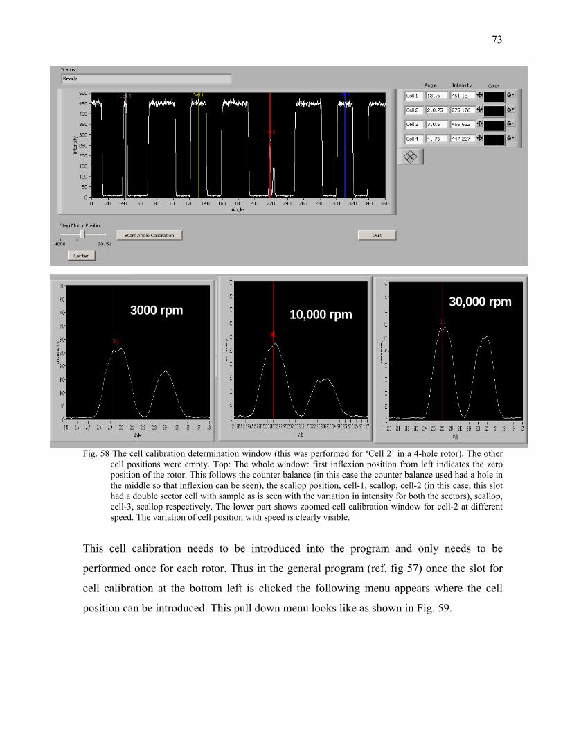
73
30,000 rpm10,000 rpm3000 rpm
Fig. 58 The cell calibration determination window (this was performed for ‘Cell 2’ in a 4-hole rotor). The other
cell positions were empty. Top: The whole window: first inflexion position from left indicates the zero position of the rotor. This follows the counter balance (in this case the counter balance used had a hole in the middle so that inflexion can be seen), the scallop position, cell-1, scallop, cell-2 (in this case, this slot had a double sector cell with sample as is seen with the variation in intensity for both the sectors), scallop, cell-3, scallop respectively. The lower part shows zoomed cell calibration window for cell-2 at different speed. The variation of cell position with speed is clearly visible.
This cell calibration needs to be introduced into the program and only needs to be
performed once for each rotor. Thus in the general program (ref. fig 57) once the slot for
cell calibration at the bottom left is clicked the following menu appears where the cell
position can be introduced. This pull down menu looks like as shown in Fig. 59.
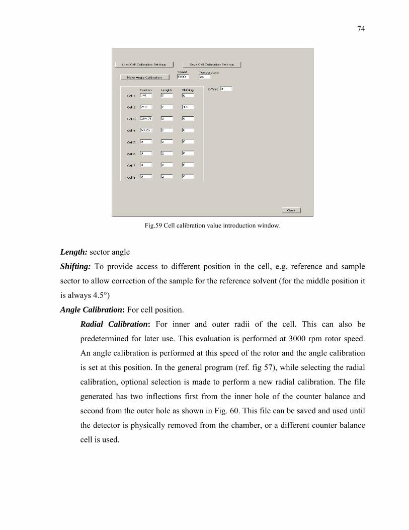
74
Fig.59 Cell calibration value introduction window.
Length: sector angle
Shifting: To provide access to different position in the cell, e.g. reference and sample
sector to allow correction of the sample for the reference solvent (for the middle position it
is always 4.5°)
Angle Calibration: For cell position.
Radial Calibration: For inner and outer radii of the cell. This can also be
predetermined for later use. This evaluation is performed at 3000 rpm rotor speed.
An angle calibration is performed at this speed of the rotor and the angle calibration
is set at this position. In the general program (ref. fig 57), while selecting the radial
calibration, optional selection is made to perform a new radial calibration. The file
generated has two inflections first from the inner hole of the counter balance and
second from the outer hole as shown in Fig. 60. This file can be saved and used until
the detector is physically removed from the chamber, or a different counter balance
cell is used.
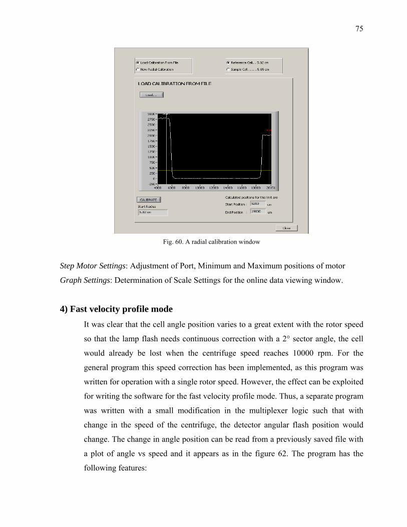
75
Fig. 60. A radial calibration window
Step Motor Settings: Adjustment of Port, Minimum and Maximum positions of motor
Graph Settings: Determination of Scale Settings for the online data viewing window.
4) Fast velocity profile mode It was clear that the cell angle position varies to a great extent with the rotor speed
so that the lamp flash needs continuous correction with a 2° sector angle, the cell
would already be lost when the centrifuge speed reaches 10000 rpm. For the
general program this speed correction has been implemented, as this program was
written for operation with a single rotor speed. However, the effect can be exploited
for writing the software for the fast velocity profile mode. Thus, a separate program
was written with a small modification in the multiplexer logic such that with
change in the speed of the centrifuge, the detector angular flash position would
change. The change in angle position can be read from a previously saved file with
a plot of angle vs speed and it appears as in the figure 62. The program has the
following features:

76
General scan parameters:
Acquisition time: This is user definable. The centrifuge can be stopped before
the final speed is reached or may be left at highest speed for longer time.
Final speed: User can select the final speed.
Radial scan parameters: User can define the radial positions for inner and outer
hole in counter balance from the radial calibration file (fig 60).
Wavelengths: The user can define the wavelengths for online data viewing with
the option to save the full spectra.
Radius: User needs define the radius position of the detector.
The general program has the following look (Fig. 61):
Fig.61 Front panel for fast velocity profiling program
Angle vs Speed Calibration: This will have to be read from a previously stored
file that can be created while the detector is installed in the first instance. For this to
be performed, the user needs to define the wavelength and angle range to avoid
undue experiment time, while covering the desired variation limit, speed range
(minimum 1000 rpm, as this is the lowest possible speed in commercial
instruments) and angle increment. An angle vs speed plot is shown in Fig. 62.
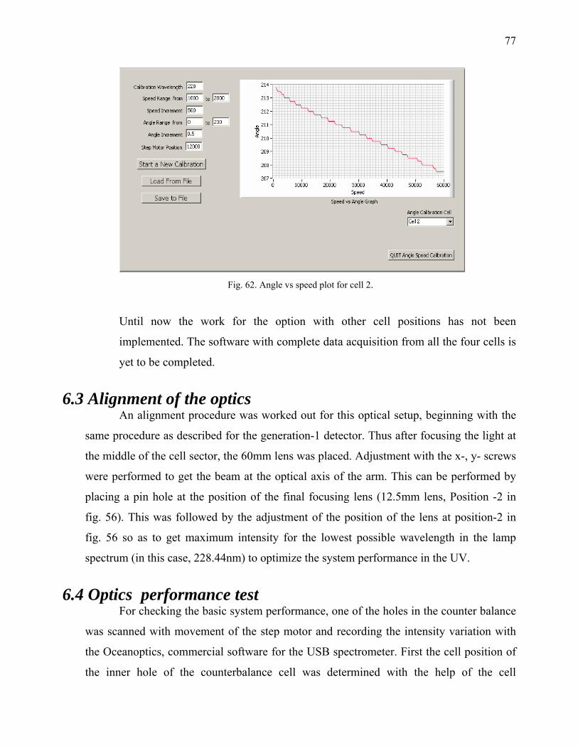
77
Fig. 62. Angle vs speed plot for cell 2.
Until now the work for the option with other cell positions has not been
implemented. The software with complete data acquisition from all the four cells is
yet to be completed.
6.3 Alignment of the optics An alignment procedure was worked out for this optical setup, beginning with the
same procedure as described for the generation-1 detector. Thus after focusing the light at
the middle of the cell sector, the 60mm lens was placed. Adjustment with the x-, y- screws
were performed to get the beam at the optical axis of the arm. This can be performed by
placing a pin hole at the position of the final focusing lens (12.5mm lens, Position -2 in
fig. 56). This was followed by the adjustment of the position of the lens at position-2 in
fig. 56 so as to get maximum intensity for the lowest possible wavelength in the lamp
spectrum (in this case, 228.44nm) to optimize the system performance in the UV.
6.4 Optics performance test For checking the basic system performance, one of the holes in the counter balance
was scanned with movement of the step motor and recording the intensity variation with
the Oceanoptics, commercial software for the USB spectrometer. First the cell position of
the inner hole of the counterbalance cell was determined with the help of the cell
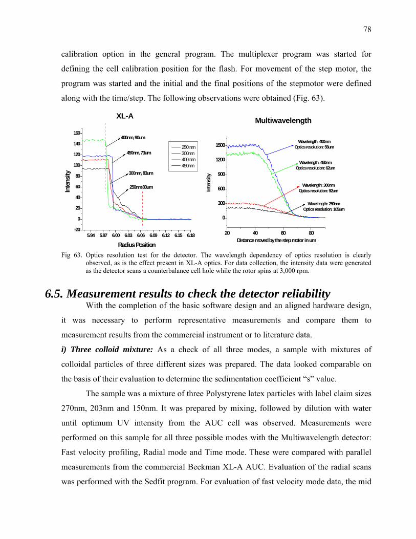
78
calibration option in the general program. The multiplexer program was started for
defining the cell calibration position for the flash. For movement of the step motor, the
program was started and the initial and the final positions of the stepmotor were defined
along with the time/step. The following observations were obtained (Fig. 63).
5.94 5.97 6.00 6.03 6.06 6.09 6.12 6.15 6.18-20
0
20
40
60
80
100
120
140
160
Inte
nsity
Radius Position
250 nm 300nm 400 nm 450nm
400nm, 90um
450nm, 73um
300nm, 83um
250nm,80um
XL-A Multiwavelength
20 40 60 80
0
300
600
900
1200
1500
Wavelength: 250nmOptics resolution: 105um
Wavelength: 300nmOptics resolution: 92um
Wavelength: 450nmOptics resolution: 62um
Inte
nsity
Distance moved by the step motor in um
Wavelength: 400nmOptics resolution: 56um
Fig 63. Optics resolution test for the detector. The wavelength dependency of optics resolution is clearly
observed, as is the effect present in XL-A optics. For data collection, the intensity data were generated as the detector scans a counterbalance cell hole while the rotor spins at 3,000 rpm.
6.5. Measurement results to check the detector reliability With the completion of the basic software design and an aligned hardware design,
it was necessary to perform representative measurements and compare them to
measurement results from the commercial instrument or to literature data.
i) Three colloid mixture: As a check of all three modes, a sample with mixtures of
colloidal particles of three different sizes was prepared. The data looked comparable on
the basis of their evaluation to determine the sedimentation coefficient “s” value.
The sample was a mixture of three Polystyrene latex particles with label claim sizes
270nm, 203nm and 150nm. It was prepared by mixing, followed by dilution with water
until optimum UV intensity from the AUC cell was observed. Measurements were
performed on this sample for all three possible modes with the Multiwavelength detector:
Fast velocity profiling, Radial mode and Time mode. These were compared with parallel
measurements from the commercial Beckman XL-A AUC. Evaluation of the radial scans
was performed with the Sedfit program. For evaluation of fast velocity mode data, the mid

79
point of the step is considered. First order differentiation can be performed on the data set
in order to accurately determine the midpoint of this step. The corresponding ω2t value is
noted for this point. A radial scan of the sedimented sample is performed to determine the
meniscus position of the sample in the cell, and all the data are substituted into the
equation s = ln (r/rm) / ω2t. The evaluation of the time mode data can also be performed in
the same way. The results obtained are summarized in table 3:
Table 3 Multiwavelength Detector data
Sample s from XL-A Radial scan (5000 rpm)
(in S)
s from Radial scan (5000rpm)
(in S)
s from fast scan mode (using
s=ln(r/rm)/ ω2t) (in S)
s from Time mode scan (using
s=ln(r/rm)/ ω2t) (in S)
270nm
1639 1624 1698 1699
203nm
935 914 1019 935
150nm
515 495 562 495
The raw data with their evaluation are shown in Fig. 64. The additional advantage of data averaging is also possible, due to the availability of large dataset.
-1000 0 1000 2000 3000 4000 5000 6000 7000 8000
0.0
0.2
0.4
0.6
0.8
1.0
1.2
Abso
rban
ce
Time in seconds
Multiwavelength detector Time mode Raw Data
400nm, 5000rpm speed, 400nm
0 50 100 150 200
0.0
0.2
0.4
0.6
0.8
1.0
1.2
Abso
rban
ce
Time in Seconds
"Abs vs Time" for Speed profile (fast velocity mode)
Fig.64 Three colloid mixture data in time mode and fast velocity profiling mode. (The detection wavelength in
both cased was: 400nm) Fig. 65 shows the comparison of evaluation of the data collected with the multiwavelength
detector and from reference XL-A experiment where data were collected for the same
sample with identical scan conditions. The evaluations show good concordance for both
evaluations. Fig. 66 shows the raw data from multiwavelength and XL-A. The presence of
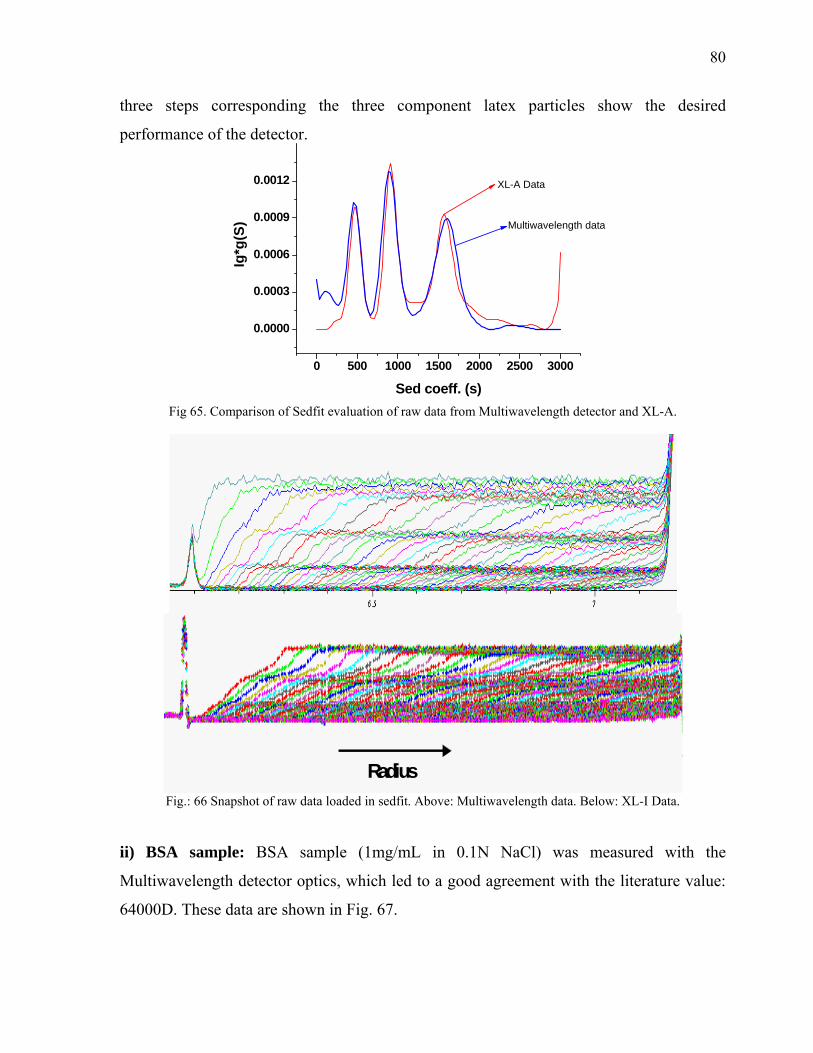
80
three steps corresponding the three component latex particles show the desired
performance of the detector.
0 500 1000 1500 2000 2500 3000
0.0000
0.0003
0.0006
0.0009
0.0012
Ig*g
(S)
Sed coeff. (s)
Multiwavelength data
XL-A Data
Fig 65. Comparison of Sedfit evaluation of raw data from Multiwavelength detector and XL-A.
Radius
Fig.: 66 Snapshot of raw data loaded in sedfit. Above: Multiwavelength data. Below: XL-I Data.
ii) BSA sample: BSA sample (1mg/mL in 0.1N NaCl) was measured with the
Multiwavelength detector optics, which led to a good agreement with the literature value:
64000D. These data are shown in Fig. 67.
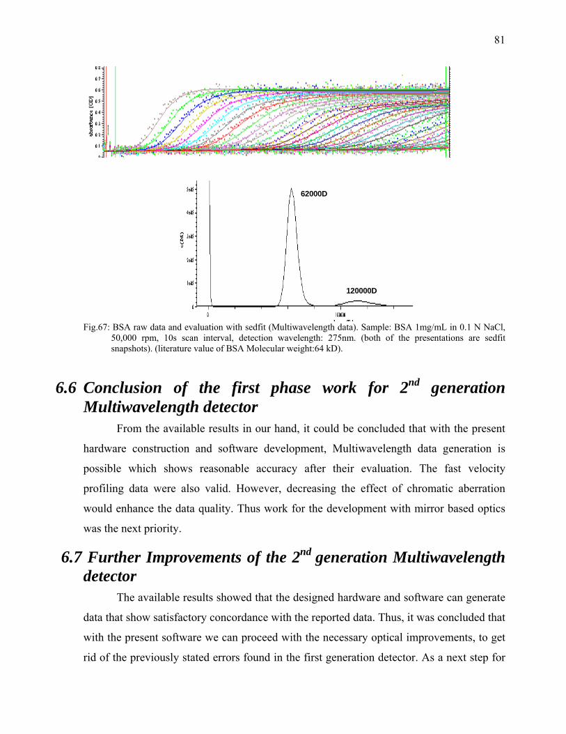
81
62000D
120000D
Fig.67: BSA raw data and evaluation with sedfit (Multiwavelength data). Sample: BSA 1mg/mL in 0.1 N NaCl,
50,000 rpm, 10s scan interval, detection wavelength: 275nm. (both of the presentations are sedfit snapshots). (literature value of BSA Molecular weight:64 kD).
6.6 Conclusion of the first phase work for 2nd generation Multiwavelength detector
From the available results in our hand, it could be concluded that with the present
hardware construction and software development, Multiwavelength data generation is
possible which shows reasonable accuracy after their evaluation. The fast velocity
profiling data were also valid. However, decreasing the effect of chromatic aberration
would enhance the data quality. Thus work for the development with mirror based optics
was the next priority.
6.7 Further Improvements of the 2nd generation Multiwavelength detector
The available results showed that the designed hardware and software can generate
data that show satisfactory concordance with the reported data. Thus, it was concluded that
with the present software we can proceed with the necessary optical improvements, to get
rid of the previously stated errors found in the first generation detector. As a next step for
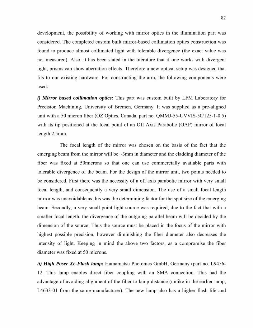
82
development, the possibility of working with mirror optics in the illumination part was
considered. The completed custom built mirror-based collimation optics construction was
found to produce almost collimated light with tolerable divergence (the exact value was
not measured). Also, it has been stated in the literature that if one works with divergent
light, prisms can show aberration effects. Therefore a new optical setup was designed that
fits to our existing hardware. For constructing the arm, the following components were
used:
i) Mirror based collimation optics: This part was custom built by LFM Laboratory for
Precision Machining, University of Bremen, Germany. It was supplied as a pre-aligned
unit with a 50 micron fiber (OZ Optics, Canada, part no. QMMJ-55-UVVIS-50/125-1-0.5)
with its tip positioned at the focal point of an Off Axis Parabolic (OAP) mirror of focal
length 2.5mm.
The focal length of the mirror was chosen on the basis of the fact that the
emerging beam from the mirror will be ~3mm in diameter and the cladding diameter of the
fiber was fixed at 50microns so that one can use commercially available parts with
tolerable divergence of the beam. For the design of the mirror unit, two points needed to
be considered. First there was the necessity of a off axis parabolic mirror with very small
focal length, and consequently a very small dimension. The use of a small focal length
mirror was unavoidable as this was the determining factor for the spot size of the emerging
beam. Secondly, a very small point light source was required, due to the fact that with a
smaller focal length, the divergence of the outgoing parallel beam will be decided by the
dimension of the source. Thus the source must be placed in the focus of the mirror with
highest possible precision, however diminishing the fiber diameter also decreases the
intensity of light. Keeping in mind the above two factors, as a compromise the fiber
diameter was fixed at 50 microns.
ii) High Poser Xe-Flash lamp: Hamamatsu Photonics GmbH, Germany (part no. L9456-
12. This lamp enables direct fiber coupling with an SMA connection. This had the
advantage of avoiding alignment of the fiber to lamp distance (unlike in the earlier lamp,
L4633-01 from the same manufacturer). The new lamp also has a higher flash life and

83
higher output stability (light output intensity variation 1.5% for this module and 5% for the
earlier one), compact modular size and a high light emission repetition rate (up to 530
Hz)147
iii)Plane mirror: 45° elliptical flat mirror coated with UV-enhanced Aluminium from
Edmund Optics Inc., Germany (part no. NT43-573).
iv)Biconvex lens: Biconvex lenses of focal length 60mm and 12.5mm were obtained from
LINOS Photonics GmbH & Co. KG, Göttingen, Germany.
v) Iris Diaphragm: From LINOS Photonics GmbH & Co. KG, Göttingen, Germany.
The other parts were equal to those described for the first generation detector: Oceanoptics
spectrometer of the USB series, Step motor for precision movement of the detector arm,
vacuum feed through for guiding the light into the vacuum chamber, x-y stage for fine
adjustment of the detection optics, and an electrical feed through for supplying power to
the step motor and connecting the computer data cable.
A schematic diagram of the optics is shown in Fig. 68:
Fig.68 The optics arm. (1) 50 micron fiber UV/Vis (OZ optics), (2) Tip of the 50micron fiber and focus of the
Off axis parabolic mirror, (3) Off axis parabolic mirror (from LFM Bremen) (4) Plane mirror (Edmunds optics) (5)Iris Diaphragm for reducing the high light intensity (6) Focusing biconvex lens (60mm), (7) Focusing biconvex lens (12.5mm), (8) Spectrometer fitted in a x-,y- stage. The light path is also shown schematically.
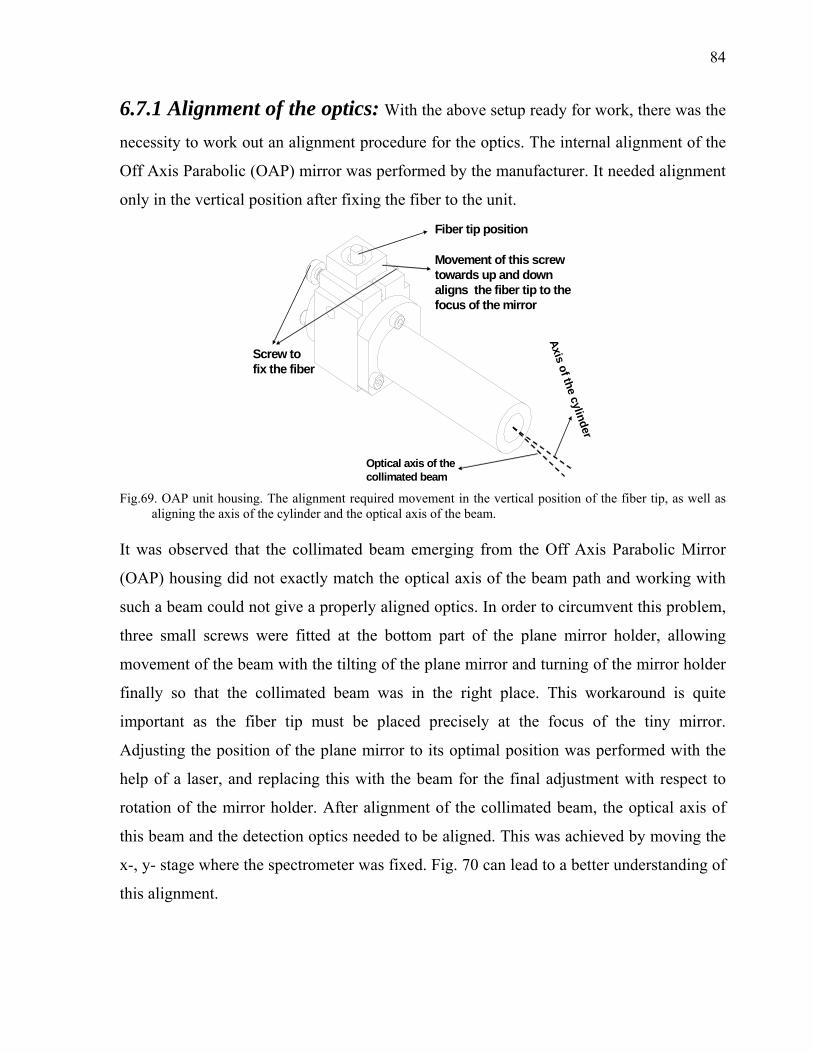
84
6.7.1 Alignment of the optics: With the above setup ready for work, there was the
necessity to work out an alignment procedure for the optics. The internal alignment of the
Off Axis Parabolic (OAP) mirror was performed by the manufacturer. It needed alignment
only in the vertical position after fixing the fiber to the unit.
Fiber tip position
Movement of this screw towards up and down aligns the fiber tip to the focus of the mirror
Screw to fix the fiber
Optical axis of the collimated beam
Axis of the cylinder
Fig.69. OAP unit housing. The alignment required movement in the vertical position of the fiber tip, as well as
aligning the axis of the cylinder and the optical axis of the beam.
It was observed that the collimated beam emerging from the Off Axis Parabolic Mirror
(OAP) housing did not exactly match the optical axis of the beam path and working with
such a beam could not give a properly aligned optics. In order to circumvent this problem,
three small screws were fitted at the bottom part of the plane mirror holder, allowing
movement of the beam with the tilting of the plane mirror and turning of the mirror holder
finally so that the collimated beam was in the right place. This workaround is quite
important as the fiber tip must be placed precisely at the focus of the tiny mirror.
Adjusting the position of the plane mirror to its optimal position was performed with the
help of a laser, and replacing this with the beam for the final adjustment with respect to
rotation of the mirror holder. After alignment of the collimated beam, the optical axis of
this beam and the detection optics needed to be aligned. This was achieved by moving the
x-, y- stage where the spectrometer was fixed. Fig. 70 can lead to a better understanding of
this alignment.

85
Mirror holder
Mirror
Plane mirror
Collimated light
Position of the screws for fine adjustment
Rotation of Holder
x y x-, y- movement of the stage screws
Spectrometer
Fig.70 Schematic description of the alignment of different optical elements.
To achieve the optimum aligned position of the two lenses in the detection optics, the lens
positions were fixed at the position of highest intensity in the spectrometer. The optical
resolution was then maximized by adjusting with the variation of the lens position in front
of the spectrometer, and finally a fine adjustment of the detection optics with respect to its
x-y movement completed the alignment.
6.7.2 Optics Performance Test i) Optics Resolution: A normal optics resolution test was performed as with the earlier
detector generation at 3000 rpm by scanning the inner hole of the counterbalance cell. The
results, shown in Fig. 71 still show that effects of chromatic aberration due to two
remaining lenses , although it is reduced significantly in comparison to the second
generation optics.

86
5.94 5.97 6.00 6.03 6.06 6.09 6.12 6.15 6.18-20
0
20
40
60
80
100
120
140
160
Inte
nsity
Radius Position
250 nm 300nm 400 nm 450nm
400nm, 90um
450nm, 73um
300nm, 83um
250nm,80um
XL-A Multiwavelength
50 100 150 200
0
200
400
600
800
1000
1200
1400
Inte
nsity
Distance moved by the step motor in µm
300nm 350nm 400nm 450nm 500nm 550nm
85um75um66um
44um48um
42um
Wavelength Resolution
Fig. 71 Optics resolution as a test for the performance of the optics. The dependence of radial resolution on
wavelength is persistent as there were two lenses in the detection optics (however decreased as compared to Generation-2). For Multiwavelength data: rotor speed 3000rpm, step size: 1um, time/step: 100us. For XL-A data, intensity scan was performed on a counter balance cell hole as the rotor spins at a speed of 3,000 rpm.
ii) Test for signal to noise: The existence of intensity variation from flash to flash. A
correction for this flash variation had been corrected in the commercial single wavelength
optics. Effort was made in the current setup to perform corrections by recording reference
intensity in a photodiode. However, this was not successful as the photodiode response to
the whole wavelength range was not the same as that from the spectrometer. The
photodiode has fixed spectral characteristics that would never be comparable to the CCD
chip detection in the spectrometer where every pixel in the CCD chip corresponds to a
particular wavelength. A rational solution would be to use a dual channel spectrometer
where a portion of the incident light to the detector may be diverted and measured as
identical signal to the spectrometer collecting the data. However, since this was evident to
us already, it was decided to perform a test in order to see the effect on the data with this
flash variation. For performing this test, the detector was moved along the sample sector at
a step size of 10µm with wait time of 100µs at rotor speed of 3000 rpm. A constant value
from the mid position of the reference sector was subtracted. The plot was generated as
‘abs.’ vs time (which in turn corresponds to the step motor position). A standard deviation
of 0.04695 (for flash intensity variation along the cell sector Fig. 72) and 0.10641 (for
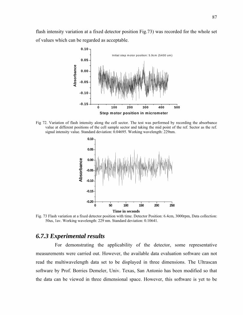
87
flash intensity variation at a fixed detector position Fig.73) was recorded for the whole set
of values which can be regarded as acceptable.
0 100 200 300 400 500-0.15
-0.10
-0.05
0.00
0.05
0.10
Abs
orba
nce
Step motor position in micrometer
In itia l step m otor position: 5.9cm (5400 um )
Fig 72. Variation of flash intensity along the cell sector. The test was performed by recording the absorbance
value at different positions of the cell sample sector and taking the mid point of the ref. Sector as the ref. signal intensity value. Standard deviation: 0.04695. Working wavelength: 229nm.
0 50 100 150 200 250-0.20
-0.15
-0.10
-0.05
0.00
0.05
0.10
Abs
orba
nce
Fig. 73 Flash variation at a fixed detector position with time. Detector Position: 6.4cm, 3000rpm, Data collection: 50us, 1av. Working wavelength: 229 nm. Standard deviation: 0.10641.
6.7.3 Experimental results For demonstrating the applicability of the detector, some representative
measurements were carried out. However, the available data evaluation software can not
read the multiwavelength data set to be displayed in three dimensions. The Ultrascan
software by Prof. Borries Demeler, Univ. Texas, San Antonio has been modified so that
the data can be viewed in three dimensional space. However, this software is yet to be
Time in seconds
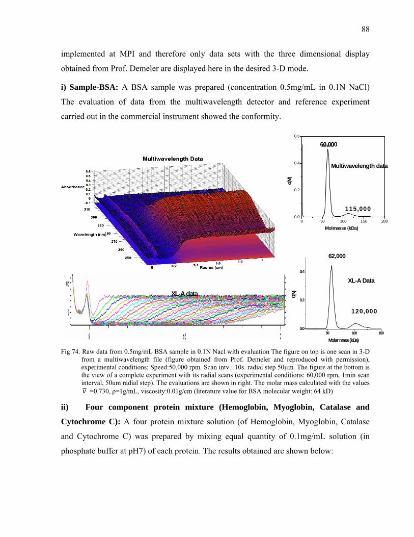
88
implemented at MPI and therefore only data sets with the three dimensional display
obtained from Prof. Demeler are displayed here in the desired 3-D mode.
i) Sample-BSA: A BSA sample was prepared (concentration 0.5mg/mL in 0.1N NaCl)
The evaluation of data from the multiwavelength detector and reference experiment
carried out in the commercial instrument showed the conformity.
0 50 100 150 2000.0
0.2
0.4
0.6
62722,32
c(M)
Molmasse (kDa)
50 100 1500.0
0.2
0.4
C(M)
Molar mass (kDa)
60,000
62000
XL-A data
62,000
Multiwavelength data
XL-A Data
120,000
115,000
Fig 74. Raw data from 0.5mg/mL BSA sample in 0.1N Nacl with evaluation The figure on top is one scan in 3-D
from a multiwavelength file (figure obtained from Prof. Demeler and reproduced with permission), experimental conditions; Speed:50,000 rpm. Scan intv.: 10s. radial step 50µm. The figure at the bottom is the view of a complete experiment with its radial scans (experimental conditions: 60,000 rpm, 1min scan interval, 50um radial step). The evaluations are shown in right. The molar mass calculated with the values v =0.730, ρ=1g/mL, viscosity:0.01g/cm (literature value for BSA molecular weight: 64 kD)
ii) Four component protein mixture (Hemoglobin, Myoglobin, Catalase and
Cytochrome C): A four protein mixture solution (of Hemoglobin, Myoglobin, Catalase
and Cytochrome C) was prepared by mixing equal quantity of 0.1mg/mL solution (in
phosphate buffer at pH7) of each protein. The results obtained are shown below:
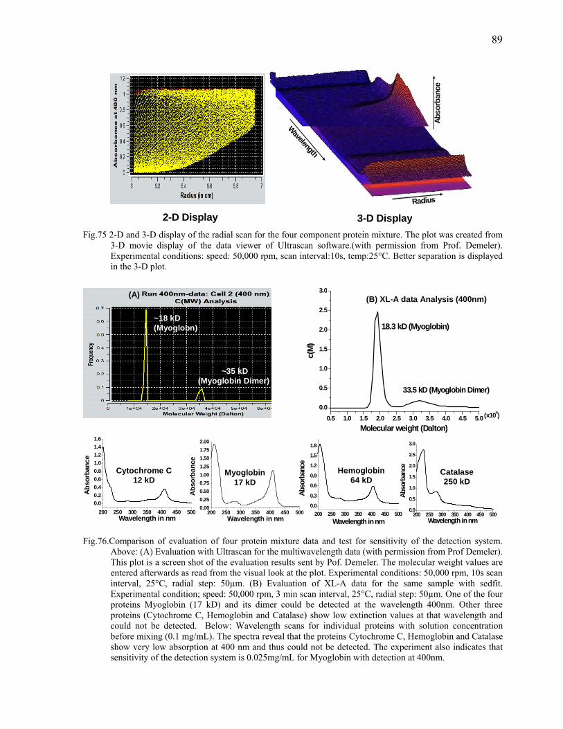
89
Abso
rban
ce
Radius
Wavelength
2-D Display 3-D Display Fig.75 2-D and 3-D display of the radial scan for the four component protein mixture. The plot was created from
3-D movie display of the data viewer of Ultrascan software.(with permission from Prof. Demeler). Experimental conditions: speed: 50,000 rpm, scan interval:10s, temp:25°C. Better separation is displayed in the 3-D plot.
~18 kD(Myoglobn)
0.5 1.0 1.5 2.0 2.5 3.0 3.5 4.0 4.5 5.00.0
0.5
1.0
1.5
2.0
2.5
3.0
c(M
)
Molecular weight (Dalton)
18.3 kD (Myoglobin)
33.5 kD (Myoglobin Dimer)
(x104)
(B) XL-A data Analysis (400nm)
200 250 300 350 400 450 5000.0
0.5
1.0
1.5
2.0
2.5
3.0
Abso
rban
ce
Wavelength in nm200 250 300 350 400 450 500
0.0
0.3
0.6
0.9
1.2
1.5
1.8
Abso
rban
ce
Wavelength in nm
Catalase250 kD
Hemoglobin 64 kD
200 250 300 350 400 450 5000.000.250.500.751.001.251.501.752.00
Abs
orba
nce
Wavelength in nm
~35 kD(Myoglobin Dimer)
Myoglobin 17 kD
200 250 300 350 400 450 5000.00.20.40.60.81.01.21.41.6
Abso
rban
ce
Wavelength in nm
Cytochrome C 12 kD
(A)
Fig.76.Comparison of evaluation of four protein mixture data and test for sensitivity of the detection system.
Above: (A) Evaluation with Ultrascan for the multiwavelength data (with permission from Prof Demeler). This plot is a screen shot of the evaluation results sent by Pof. Demeler. The molecular weight values are entered afterwards as read from the visual look at the plot. Experimental conditions: 50,000 rpm, 10s scan interval, 25°C, radial step: 50µm. (B) Evaluation of XL-A data for the same sample with sedfit. Experimental condition; speed: 50,000 rpm, 3 min scan interval, 25°C, radial step: 50µm. One of the four proteins Myoglobin (17 kD) and its dimer could be detected at the wavelength 400nm. Other three proteins (Cytochrome C, Hemoglobin and Catalase) show low extinction values at that wavelength and could not be detected. Below: Wavelength scans for individual proteins with solution concentration before mixing (0.1 mg/mL). The spectra reveal that the proteins Cytochrome C, Hemoglobin and Catalase show very low absorption at 400 nm and thus could not be detected. The experiment also indicates that sensitivity of the detection system is 0.025mg/mL for Myoglobin with detection at 400nm.

90
The results presented above clearly show that better separation of components can be
visualized with a 3-D data display. Also, the user can select any wavelength in the range of
200-800nm for separate evaluation. These are clear advantages over existing commercial
instruments as the user can see the raw data in 3-D space so as to select the wavelength for
evaluation. Also, the presence of data sets for the whole wavelength range allows the user
to perform the evaluation at the selected wavelength. For working wavelength of 400nm,
one of the four proteins Myoglobin (and its dimer) could be detected as other three show
low extinction at that wavelength. The experiment can also give information about the
sensitivity of the detection system, a 0.025mg/mL Myoglobin solution in phosphate buffer
at pH: 7 is satisfactorily detectable at 400nm. The other three proteins could not be
detected for the same solution concentration at 400nm.
ii) Quantum size effect study for TiO2 particles: It is a well known fact that TiO2
particles show the Q-size effect. In the past the particle size characterization of TiO2 or
other samples showing these effects, involved time consuming experimental work.
Determining the relation between band gap and particle size involved synthesis of
monodisperse particles of defined size, their particle size determination (usually by TEM)
and then UV/Vis characterization. This time consuming analysis work can be done by a
single experiment in Multiwavelength detection AUC. The radial scans can be used for
establishing this because as the particles are fractionated in the centrifugal field, a shift in
the wavelength maxima for different particles can be simultaneously observed, as shown
in Fig. 77. In commercially available instruments, in order to demonstrate the same effect
one needs to carry out wavelength scan at different radial positions (Fig. 78), which is also
a time consuming experiment and risks a loss of information as data enrichment is rather
slow.
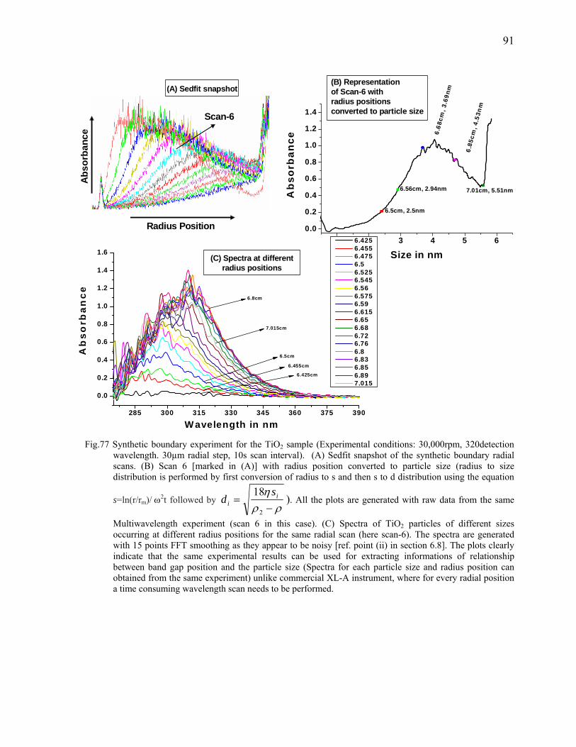
91
1 2 3 4 5 60.0
0.2
0.4
0.6
0.8
1.0
1.2
1.4
Ab
sorb
ance
Size in nm
6.5cm, 2.5nm
6.56cm, 2.94nm
6.68
cm, 3
.69n
m
6.85
cm, 4
.53n
m
7.01cm, 5.51nm
285 300 315 330 345 360 375 390
0.0
0.2
0.4
0.6
0.8
1.0
1.2
1.4
1.6
Ab
sorb
ance
W avelength in nm
6.425 6.455 6.475 6.5 6.525 6.545 6.56 6.575 6.59 6.615 6.65 6.68 6.72 6.76 6.8 6.83 6.85 6.89 7.015
6.425cm
7.015cm
6.8cm
6.455cm
6.5cm
Abso
rban
ce
Radius Position
Scan-6
(A) Sedfit snapshot(B) Representation of Scan-6 with radius positions converted to particle size
(C) Spectra at different radius positions
Fig.77 Synthetic boundary experiment for the TiO2 sample (Experimental conditions: 30,000rpm, 320detection
wavelength. 30µm radial step, 10s scan interval). (A) Sedfit snapshot of the synthetic boundary radial scans. (B) Scan 6 [marked in (A)] with radius position converted to particle size (radius to size distribution is performed by first conversion of radius to s and then s to d distribution using the equation
s=ln(r/rm)/ ω2t followed by ρρ
η−
=2
18 ii
sd ). All the plots are generated with raw data from the same
Multiwavelength experiment (scan 6 in this case). (C) Spectra of TiO2 particles of different sizes occurring at different radius positions for the same radial scan (here scan-6). The spectra are generated with 15 points FFT smoothing as they appear to be noisy [ref. point (ii) in section 6.8]. The plots clearly indicate that the same experimental results can be used for extracting informations of relationship between band gap position and the particle size (Spectra for each particle size and radius position can obtained from the same experiment) unlike commercial XL-A instrument, where for every radial position a time consuming wavelength scan needs to be performed.
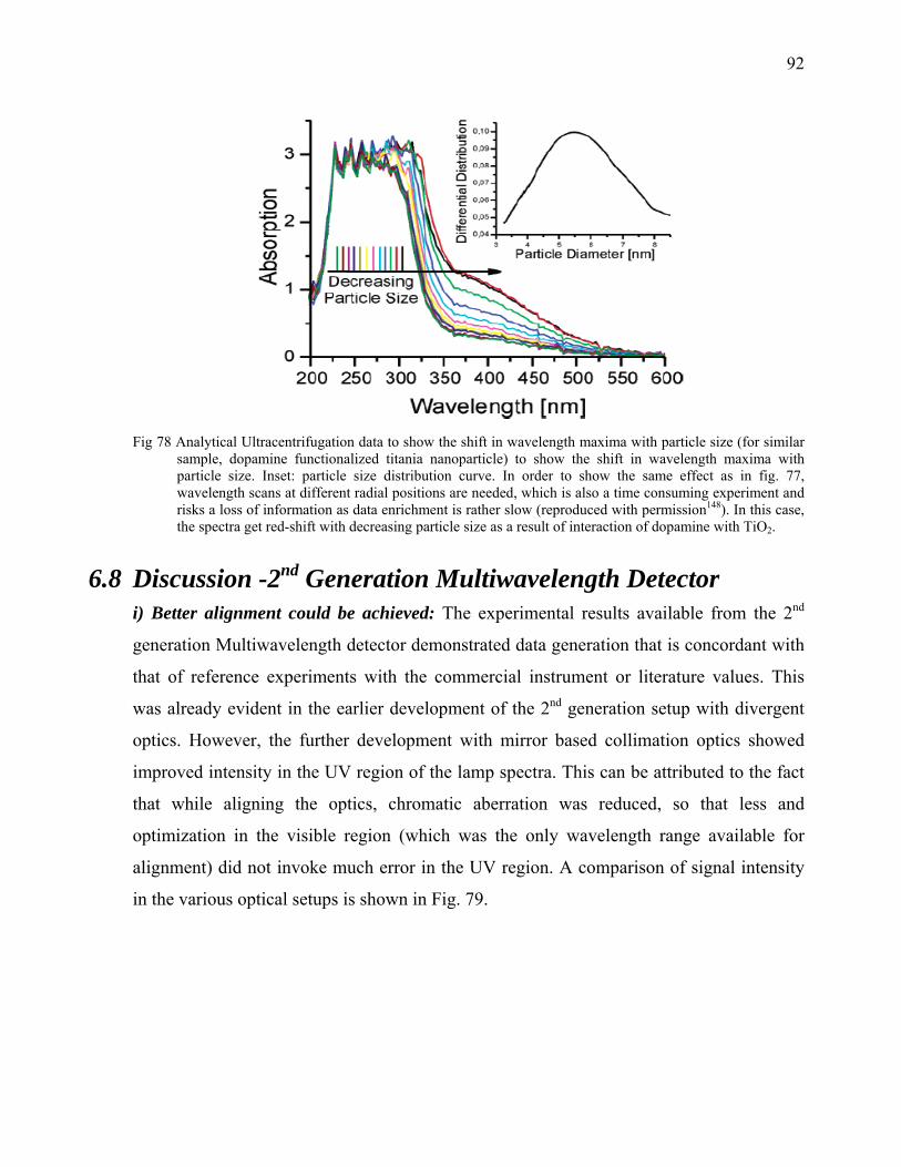
92
Fig 78 Analytical Ultracentrifugation data to show the shift in wavelength maxima with particle size (for similar
sample, dopamine functionalized titania nanoparticle) to show the shift in wavelength maxima with particle size. Inset: particle size distribution curve. In order to show the same effect as in fig. 77, wavelength scans at different radial positions are needed, which is also a time consuming experiment and risks a loss of information as data enrichment is rather slow (reproduced with permission148). In this case, the spectra get red-shift with decreasing particle size as a result of interaction of dopamine with TiO2.
6.8 Discussion -2nd Generation Multiwavelength Detector i) Better alignment could be achieved: The experimental results available from the 2nd
generation Multiwavelength detector demonstrated data generation that is concordant with
that of reference experiments with the commercial instrument or literature values. This
was already evident in the earlier development of the 2nd generation setup with divergent
optics. However, the further development with mirror based collimation optics showed
improved intensity in the UV region of the lamp spectra. This can be attributed to the fact
that while aligning the optics, chromatic aberration was reduced, so that less and
optimization in the visible region (which was the only wavelength range available for
alignment) did not invoke much error in the UV region. A comparison of signal intensity
in the various optical setups is shown in Fig. 79.
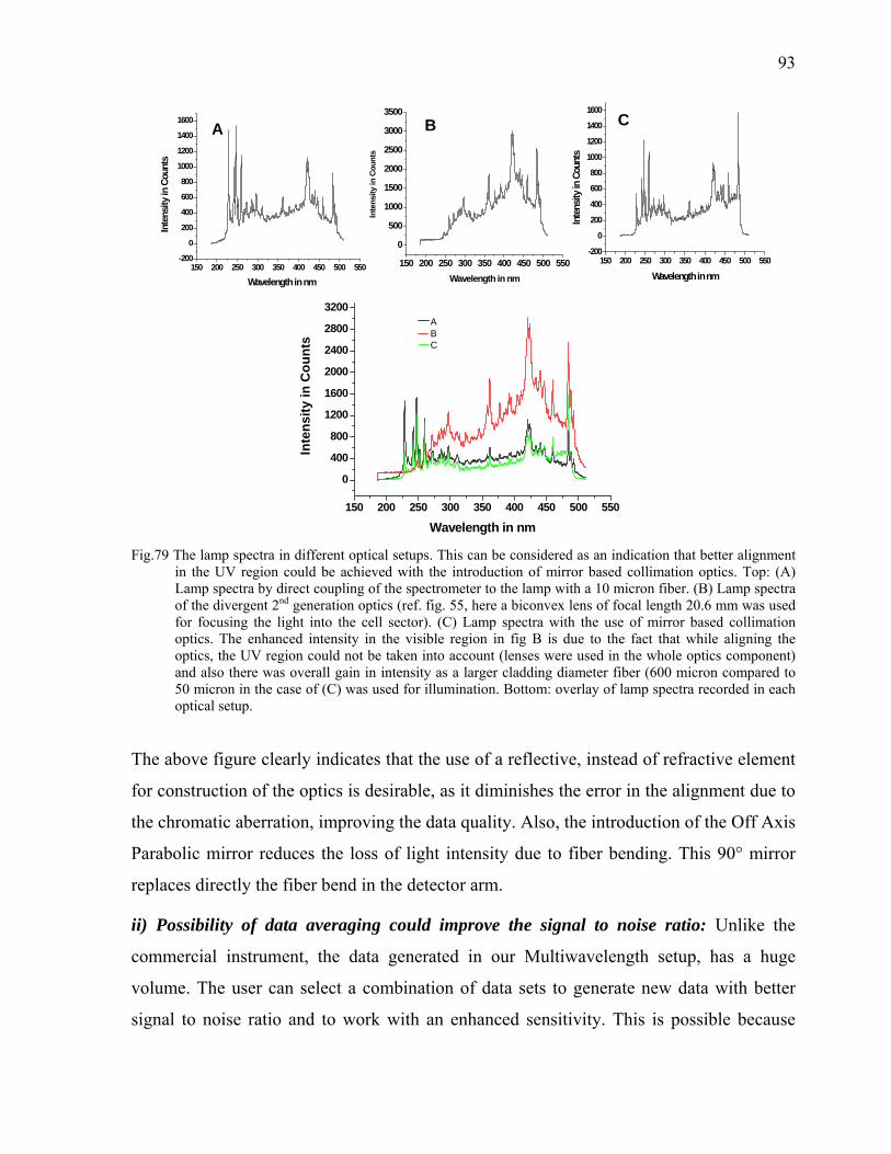
93
150 200 250 300 350 400 450 500 550-200
0
200
400
600
800
1000
1200
1400
1600
Inte
nsity
in C
ount
s
Wavelength in nm150 200 250 300 350 400 450 500 550
-200
0
200
400
600
800
1000
1200
1400
1600
Inte
nsity
in C
ount
s
Wavelength in nm
150 200 250 300 350 400 450 500 550
0
500
1000
1500
2000
2500
3000
3500
Inte
nsity
in C
ount
s
Wavelength in nm
A B C
150 200 250 300 350 400 450 500 550
0
400
800
1200
1600
2000
2400
2800
3200In
tens
ity in
Cou
nts
Wavelength in nm
ABC
Fig.79 The lamp spectra in different optical setups. This can be considered as an indication that better alignment
in the UV region could be achieved with the introduction of mirror based collimation optics. Top: (A) Lamp spectra by direct coupling of the spectrometer to the lamp with a 10 micron fiber. (B) Lamp spectra of the divergent 2nd generation optics (ref. fig. 55, here a biconvex lens of focal length 20.6 mm was used for focusing the light into the cell sector). (C) Lamp spectra with the use of mirror based collimation optics. The enhanced intensity in the visible region in fig B is due to the fact that while aligning the optics, the UV region could not be taken into account (lenses were used in the whole optics component) and also there was overall gain in intensity as a larger cladding diameter fiber (600 micron compared to 50 micron in the case of (C) was used for illumination. Bottom: overlay of lamp spectra recorded in each optical setup.
The above figure clearly indicates that the use of a reflective, instead of refractive element
for construction of the optics is desirable, as it diminishes the error in the alignment due to
the chromatic aberration, improving the data quality. Also, the introduction of the Off Axis
Parabolic mirror reduces the loss of light intensity due to fiber bending. This 90° mirror
replaces directly the fiber bend in the detector arm.
ii) Possibility of data averaging could improve the signal to noise ratio: Unlike the
commercial instrument, the data generated in our Multiwavelength setup, has a huge
volume. The user can select a combination of data sets to generate new data with better
signal to noise ratio and to work with an enhanced sensitivity. This is possible because

94
multiple wavelength data sets are acquired for each radial scan of the sedimenting species.
This is even possible for peak wavelengths in a spectrum. An example is shown in figure
80.
0 25 50 75 100 125 150 175 200 225
0.0
0.2
0.4
0.6
0.8
1.0
1.2
Abs
orba
nce
Time in Seconds
Data before averaging
Wavelength: 400 nm
Radius Position: 6.5 cm
0 25 50 75 100 125 150 175 200 225
0.0
0.2
0.4
0.6
0.8
1.0
1.2
Abs
orba
nce
Time in secdonds
Data averaged over wavelength range395.12nm to 405.95nm ( 31 points)
Mean wavelength: 400.15nm
Radius position: 6.5cm
Data after averagingA) B)
6.0 6.2 6.4 6.6 6.8 7.0 7.2-0.20.00.20.40.60.81.01.21.41.61.8
Abs
orba
nce
Radius position in cm
Radial scan before averaging
Wavelength: 229.11 nm
Speed: 50,000 rpmScan interval: 10sStep: 50µm
C)
6.0 6.2 6.4 6.6 6.8 7.0-0.20.00.20.40.60.81.01.21.41.61.8
Abs
orba
nce
Radius Position in cm
Radial scan after averaging
Speed: 50,000 rpmScan Interval: 10sStep size: µm
Data averaged in the wavelength value 229.241nm to 230.921nm (11 points)
D)
Fig. 80. Improvement in data quality with averaging. This feature can be implemented for data generated with
Multiwavelength detector as the data set contains whole UV/Vis range of wavelength. The upper half of the figure shows averaging of a fast mode velocity profile data set for a sample with three latexes mixed and diluted to give optimum UV intensity. A) Raw data for single wavelength B) Data averaged over 31 wavelength points. The lower half of the data shows the same effect for a radial scan. The scan was taken from the sample of a four protein mixture. C) Radial scan for a single wavelength from the multiwavelength data set (229.11nm). D) Data averaged over 11 wavelength points.
iii) Necessary improvement of the data acquisition software: As shown in Fig. 81, the
Multiwavelength data generated with our multiplexer and step motor control program
showed significant noise compared with data generated from our written program, and
those generated with the use of commercial software.
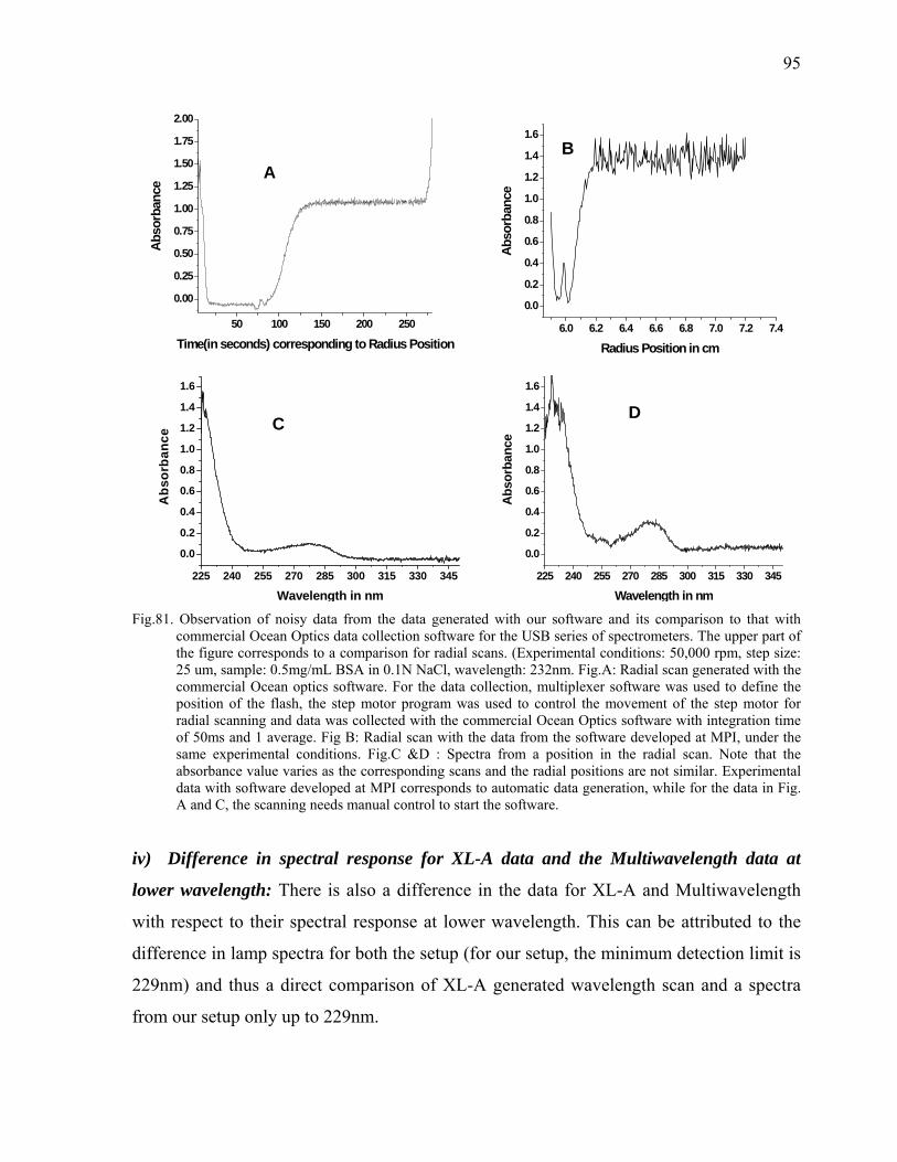
95
6.0 6.2 6.4 6.6 6.8 7.0 7.2 7.4
0.0
0.2
0.4
0.6
0.8
1.0
1.2
1.4
1.6
Abso
rban
ce
Radius Position in cm
50 100 150 200 250
0.00
0.25
0.50
0.75
1.00
1.25
1.50
1.75
2.00
Abso
rban
ce
Time(in seconds) corresponding to Radius Position
225 240 255 270 285 300 315 330 345
0.0
0.2
0.4
0.6
0.8
1.0
1.2
1.4
1.6
Abs
orba
nce
Wavelength in nm225 240 255 270 285 300 315 330 345
0.0
0.2
0.4
0.6
0.8
1.0
1.2
1.4
1.6
Abso
rban
ce
Wavelength in nm
AB
C D
Fig.81. Observation of noisy data from the data generated with our software and its comparison to that with
commercial Ocean Optics data collection software for the USB series of spectrometers. The upper part of the figure corresponds to a comparison for radial scans. (Experimental conditions: 50,000 rpm, step size: 25 um, sample: 0.5mg/mL BSA in 0.1N NaCl, wavelength: 232nm. Fig.A: Radial scan generated with the commercial Ocean optics software. For the data collection, multiplexer software was used to define the position of the flash, the step motor program was used to control the movement of the step motor for radial scanning and data was collected with the commercial Ocean Optics software with integration time of 50ms and 1 average. Fig B: Radial scan with the data from the software developed at MPI, under the same experimental conditions. Fig.C &D : Spectra from a position in the radial scan. Note that the absorbance value varies as the corresponding scans and the radial positions are not similar. Experimental data with software developed at MPI corresponds to automatic data generation, while for the data in Fig. A and C, the scanning needs manual control to start the software.
iv) Difference in spectral response for XL-A data and the Multiwavelength data at
lower wavelength: There is also a difference in the data for XL-A and Multiwavelength
with respect to their spectral response at lower wavelength. This can be attributed to the
difference in lamp spectra for both the setup (for our setup, the minimum detection limit is
229nm) and thus a direct comparison of XL-A generated wavelength scan and a spectra
from our setup only up to 229nm.
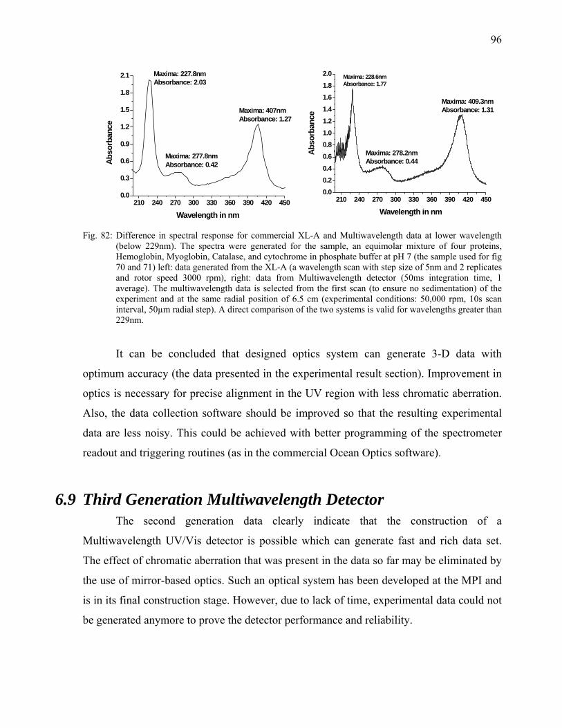
96
210 240 270 300 330 360 390 420 4500.0
0.3
0.6
0.9
1.2
1.5
1.8
2.1 Maxima: 227.8nmAbsorbance: 2.03
Maxima: 277.8nmAbsorbance: 0.42Ab
sorb
ance
Wavelength in nm
Maxima: 407nmAbsorbance: 1.27
210 240 270 300 330 360 390 420 4500.00.20.40.60.81.01.21.41.61.82.0 Maxima: 228.6nm
Absorbance: 1.77
Maxima: 278.2nmAbsorbance: 0.44
Maxima: 409.3nmAbsorbance: 1.31
Abso
rban
ce
Wavelength in nm
Fig. 82: Difference in spectral response for commercial XL-A and Multiwavelength data at lower wavelength (below 229nm). The spectra were generated for the sample, an equimolar mixture of four proteins, Hemoglobin, Myoglobin, Catalase, and cytochrome in phosphate buffer at pH 7 (the sample used for fig 70 and 71) left: data generated from the XL-A (a wavelength scan with step size of 5nm and 2 replicates and rotor speed 3000 rpm), right: data from Multiwavelength detector (50ms integration time, 1 average). The multiwavelength data is selected from the first scan (to ensure no sedimentation) of the experiment and at the same radial position of 6.5 cm (experimental conditions: 50,000 rpm, 10s scan interval, 50µm radial step). A direct comparison of the two systems is valid for wavelengths greater than 229nm.
It can be concluded that designed optics system can generate 3-D data with
optimum accuracy (the data presented in the experimental result section). Improvement in
optics is necessary for precise alignment in the UV region with less chromatic aberration.
Also, the data collection software should be improved so that the resulting experimental
data are less noisy. This could be achieved with better programming of the spectrometer
readout and triggering routines (as in the commercial Ocean Optics software).
6.9 Third Generation Multiwavelength Detector The second generation data clearly indicate that the construction of a
Multiwavelength UV/Vis detector is possible which can generate fast and rich data set.
The effect of chromatic aberration that was present in the data so far may be eliminated by
the use of mirror-based optics. Such an optical system has been developed at the MPI and
is in its final construction stage. However, due to lack of time, experimental data could not
be generated anymore to prove the detector performance and reliability.

97
A new heat sink modification was performed keeping in mind the fact that the
Beckman warranty is lost with the drilling of holes into the heat sink, which was a
disadvantage of the first and second generation detector set-up. Also, repair of feed-
throughs is difficult with the existing design as this needs removal of the can from the
vacuum chamber, which often gives rise to the problem of breaking of the Peltier elements
below the can. In order to circumvent this, a new design modification was developed for
the heat sink using the Analytical XL-I platform. To draw in the fibers and the electrical
cables, a hole in the socket for fitting the monochromator in the XL-I was utilized (In the
commercial XL-I Ultracentrifuge, light from the Xe flash lamp emerges through this hole
towards the toroidal mirror). A cut on the can was performed with the possibility to
accommodate the detector arm and its movement for radial scanning. The new heat sink
modification allows for working with the lens based arm as in the second generation, as
well as the newly designed mirror-based detector optics arm. It is a modular system, which
maintains the Beckman warranty and allows modifications without intrusion into the
instrument.
The third generation detector arm can be constructed using some commercially
available components in addition to some components already used in the second
generation detector. For the final construction of the detector arm, the collimation optics,
plane mirror for deflecting the collimated beam at·90° angle and guiding it through the cell
sector, the spectrometer and precision slit for defining the spatial resolution of the detector
were used as in the second generation optics. In addition, the following commercially
available components were used for complete construction of the optics arm in
conjunction with the above mentioned parts:
i) Four fiber vacuum feed through: This feed through is equipped with two fibers of
cladding diameter 50 microns and two fibers of cladding diameter 1000 microns.
The 50 micron fibers are to be used for the collimation optics as this cladding
diameter is pre-requisite for the construction of this optics (as discussed earlier). The
1000 micron fibers can be used for the detection optics as the light emerging from
the optics has a diminished intensity compared to the incoming light. This vacuum
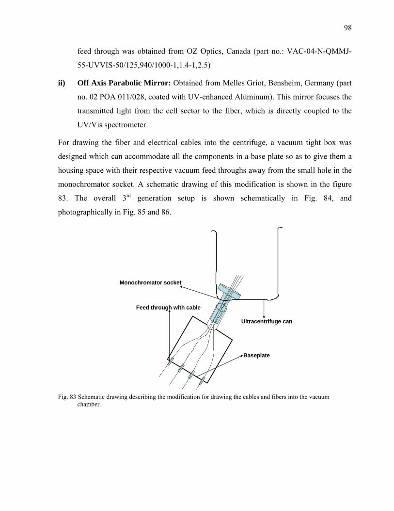
98
feed through was obtained from OZ Optics, Canada (part no.: VAC-04-N-QMMJ-
55-UVVIS-50/125,940/1000-1,1.4-1,2.5)
ii) Off Axis Parabolic Mirror: Obtained from Melles Griot, Bensheim, Germany (part
no. 02 POA 011/028, coated with UV-enhanced Aluminum). This mirror focuses the
transmitted light from the cell sector to the fiber, which is directly coupled to the
UV/Vis spectrometer.
For drawing the fiber and electrical cables into the centrifuge, a vacuum tight box was
designed which can accommodate all the components in a base plate so as to give them a
housing space with their respective vacuum feed throughs away from the small hole in the
monochromator socket. A schematic drawing of this modification is shown in the figure
83. The overall 3rd generation setup is shown schematically in Fig. 84, and
photographically in Fig. 85 and 86.
Monochromator socket
Feed through with cable
Ultracentrifuge can
Baseplate
Fig. 83 Schematic drawing describing the modification for drawing the cables and fibers into the vacuum
chamber.

99
Scheme of optics setup and photographs showing its mounting (3rd generation)
Fig. 84 The third generation optics arm. (1) 50 micron fiber (UV/Vis from the vacuum feed through), (2) Tip of
the 50micron fiber and focus of the OAP, (3) Off axis parabolic mirror (from LFM Bremen) (4) Plane mirror (Edmunds optics) (5)Focusing OAP (6) 25µm Precision slit (7) 1000 micron UV/Vis fiber (from the vacuum feed through), (8) Spectrometer. The light path is also shown schematically.
A
Cut performed on the can to fit the detector optics
BB
Housing for the feed throughs Feed through fitted to the base plate
C
Fig. 85 Photographs showing the modification of the can for fitting the detector arm and modification for drawing the cables
into the vacuum chamber. Fig A shows the view of the can from the top. Fig B and C show the housing constructed to be fitted for drawing cables inside the vacuum chamber.
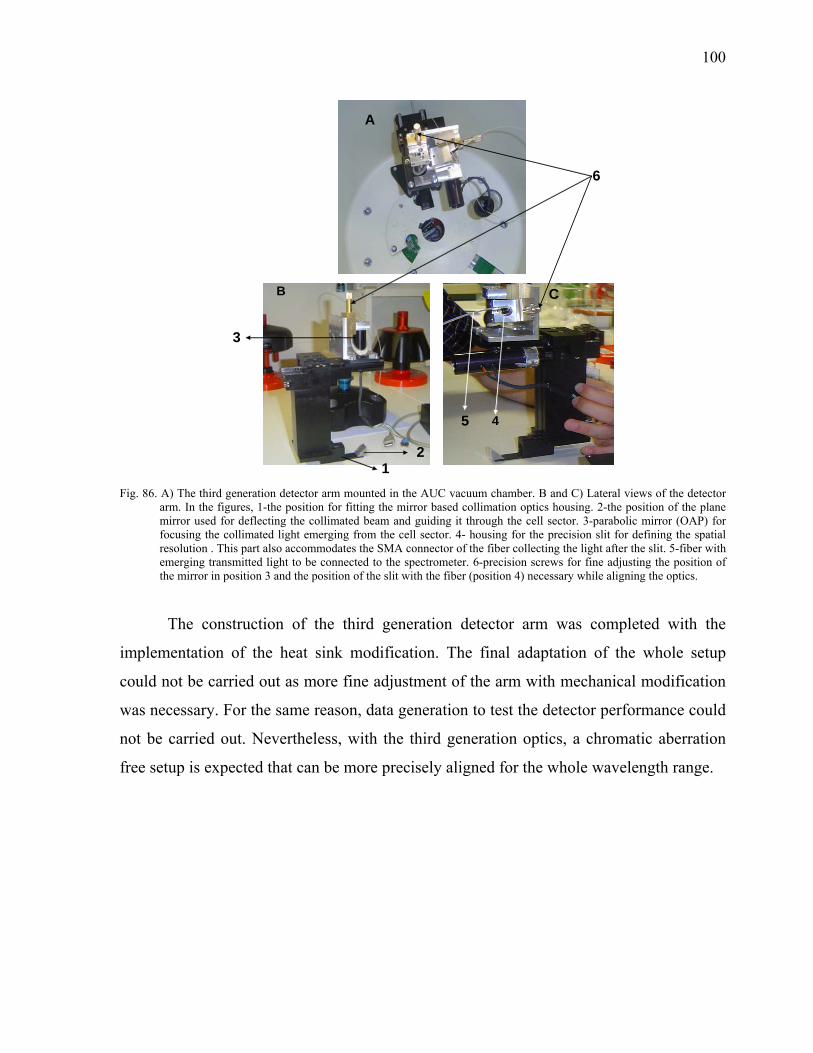
100
A
B C
3
21
4
6
5
Fig. 86. A) The third generation detector arm mounted in the AUC vacuum chamber. B and C) Lateral views of the detector
arm. In the figures, 1-the position for fitting the mirror based collimation optics housing. 2-the position of the plane mirror used for deflecting the collimated beam and guiding it through the cell sector. 3-parabolic mirror (OAP) for focusing the collimated light emerging from the cell sector. 4- housing for the precision slit for defining the spatial resolution . This part also accommodates the SMA connector of the fiber collecting the light after the slit. 5-fiber with emerging transmitted light to be connected to the spectrometer. 6-precision screws for fine adjusting the position of the mirror in position 3 and the position of the slit with the fiber (position 4) necessary while aligning the optics.
The construction of the third generation detector arm was completed with the
implementation of the heat sink modification. The final adaptation of the whole setup
could not be carried out as more fine adjustment of the arm with mechanical modification
was necessary. For the same reason, data generation to test the detector performance could
not be carried out. Nevertheless, with the third generation optics, a chromatic aberration
free setup is expected that can be more precisely aligned for the whole wavelength range.

101
Chapter-7
7.1 Conclusion
In this work approaches for development of a new detection system for the
Analytical Ultracentrifuge (AUC) were explored. Unlike its counterpart in
chromatography fractionation techniques, Multidetection system for AUC has not yet been
fully implemented. However, many applications can be foreseen for such Multidetection
capability. In this study we tried to couple existing fundamental spectroscopic and
scattering techniques, that are used in day to day science as tools for extracting analyte
information, into such an AUC detector. Trials were performed to employ Raman, small
angle laser light scattering and an improved UV/Vis detection incorporating the possibility
to work with the whole range of wavelengths, to study analyte behaviour during
ultracentrifugation experiments. Conclusions were drawn for the applicability of Raman
detector for AUC, that for such a detection system to work one needs to employ very high
power laser. It was also realized that for a Small Angle Laser Light Scattering detector,
sensitive photosensors with large active area like APD should be incorporated. The
development for a fast fiber optics based multiwavelength detector was completed.
It became obvious that with the generation of data in 3-D space in a UV/Vis
detection system, the user can select the wavelength for evaluation after completion of an
experiment. This allows evaluation of results that supplies more information, an
application which can be cited, e.g. for studying protein interactions where the individual
protein before interaction absorbs at one wavelength, that changes to another value after
their association (This applicability was proven with successful Multiwavelength detection
of a four component protein mixture). In current commercial instruments the user can
work with only three selected wavelengths. Users’ software (Sedvel), however, offers the
option to evaluate data with many wavelengths, which is not available in a data set from
XL-A. For this experimental demand, a Multiwavelength detector can satisfy a
requirement of the AUC user community as the data set contains information from all
wavelengths in the range 230-800nm. The detector construction was completed with a
lens-based modular design. Software programming and a proper alignment procedure for

102
this optical system were also performed. The data generated with this system was
evaluated with normal evaluation software used by the AUC community (Sedfit and
Ultrascan) which showed their concordance with reference measurements and literature
values. Also, the capability of much faster data generation unlike that possible with
commercial instruments was demonstrated, by collecting data for a sedimentation velocity
experiment using a mixture of three latexes. The results shown were similar to those of a
commercial instrument, whereas the experiment time for our designed optics was ~3
minutes, while the same experiment took ~2hours in the commercial instrument. This fast
mode of data generation can be used for detection of aggregates which sediment in the
early phase of an experiment and with maximum diffusion suppression (this experiment
needs a longer time and much more careful measurement in commercial XL-A). Unlike
the XL-A, data generation with wavelength resolution allows a wavelength scan at every
radial position. This is useful e.g. for demonstrating the Q-size effect for a sample. In the
present XL-A setup, in order to demonstrate this effect, a time consuming wavelength scan
is necessary at various radial positions, which in our setup is automatically generated
while performing a normal radial scan. Thus such an experiment does not require any extra
effort from the user, and a complete set of spectra for different particle sizes are available
from a single radial scan, which contains a number of spectra many times higher than can
be generated from an XL-A wavelength scan. Also, the introduction of the time mode scan
makes the detection system more versatile. This mode can be used for aggregate
determination as they tend to sediment at the beginning of an experiment. The data
averaging option can lead to better raw data visualization and also better fitting for global
analysis.
7.2 Detector development in Analytical Ultracentrifuge-A future outlook
Although the AUC user community is quite small, for some areas of research and
industrial applications, such as for determination of particle size distribution of polymers
and dispersions or for interaction studies of proteins, the technique remains unequivocal
However, the lack of appropriate detectors is often a disadvantage of present analytical
ultracentrifugation. The existing detection systems are not very precise, not fast enough,

103
and data acquisition is often not really “online”. Though the existing interference system is
fast, it lacks precision. Thus to meet the experimental expectations for AUC, it is
necessary to design and develop new detection systems. The need for new detection
systems has been well documented82, 83, 84.
There have been few efforts for developing new detection systems in AUC.
Improvements in existing detector systems can be accomplished by enhancing data
acquisition speed or data precision by application of sensitive and high resolution devices
(PMT, Avalanche photodiode, High resolution CCD cameras), or reduction of noise by
signal averaging. However, this would only increase the data quality and not the amount of
complimentary data, which could be used for the full description of a system under
investigation in a global analysis approach.
A rationale for new detection systems can be put forward with reference to
Svedberg equation:
M = sRT / D(1- v ρ0)
Ideally, introduction of a Multidetection system in AUC should allow that all the
quantities in the Svedberg equation can be simultaneously determined from a single
experiment. The experimental setup available allows determination of s and other
quantities need to be determined by using different techniques. However introduction of a
Laser Doppler Anemometry (LDA) detector in AUC can enable determination of s without
any knowledge of cell dimensions (e.g. the meniscus position, radius and bottom position)
and also for a single particle. A Small Angle Laser Light scattering (SLS) detection system
can be used for the determination of M in the above equation. With the introduction of a
Dynamic Light Scattering (DLS) detector, D can be measured. A preliminary test with a
pulsed laser already showed that the determination of the particle size is possible with
short illumination times. All of these quantities would be available as distributions. The
solution of the Svedberg equation with the three quantities available so far can yield the
density (VBAR) distribution of the sample. Also, invoking a Raman detection system to
AUC, can serve as the vital step for supplying information about the chemistry of the
components in a complex mixture. In addition, development of fast data generation
capability for the detection system shortens experiment time and enriches experimental

104
data with more valuable information, as with such a system the process of sedimentation
can be followed in more detail. Our experiment with the fast Multiwavelength detector has
already proven that such a system is possible and as many as seven samples can be
characterized in less than three minutes time.
It may be mentioned that adaptation of recent commercial products can enhance the
detector performance manifold, as has also been proven in our study to adopt a CCD-
based spectrometer for the Multiwavelength detector. Another example may be the design
of a plug and play system for SLS and LDA. Implementation of an LDA system to AUC
will be quite valuable as it can allow online measurement of the sedimentation coefficient.
LDA works on the principle that, when a particle passes through intersection volume
formed by the two coherent laser beams, the scattered light, received by a detector, has
components from both beams which interfere on the surface of the detector. Due to
changes in the difference between the optical path lengths of the two components, this
interference produces pulsating light intensity, as the particle moves through the
measurement volume, which is related to the velocity of the particle. Measurement of this
velocity can enable determination of s (using the equation u/ ω2r ≡ s), which in turn can be
related to the particle size. As the equation does not contain any term for cell dimension, s
can be determined without the knowledge of these. Also, since the determination of the
particle velocity (u) is online, the s can also be determined online. The design could use a
commercially available modular LDA probe149 that can be easily fitted to a detector arm as
was used in our Multiwavelength study. A scheme of the envisaged design is shown in
Fig. 87:
AUC Cell sector
LDA Probe
Backscattered light
Measuring volume
Detector
Bragg Cell
LAS
ER
Fig.87. LDA set up for AUC in backscattering mode.
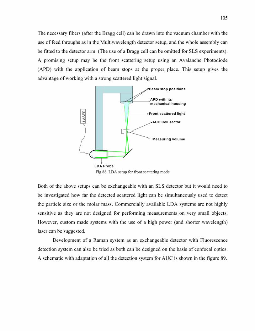
105
The necessary fibers (after the Bragg cell) can be drawn into the vacuum chamber with the
use of feed throughs as in the Multiwavelength detector setup, and the whole assembly can
be fitted to the detector arm. (The use of a Bragg cell can be omitted for SLS experiments).
A promising setup may be the front scattering setup using an Avalanche Photodiode
(APD) with the application of beam stops at the proper place. This setup gives the
advantage of working with a strong scattered light signal.
AUC Cell sector
Measuring volume
LASE
RBeam stop positions
APD with its mechanical housing
Front scattered light
LDA Probe Fig.88. LDA setup for front scattering mode
Both of the above setups can be exchangeable with an SLS detector but it would need to
be investigated how far the detected scattered light can be simultaneously used to detect
the particle size or the molar mass. Commercially available LDA systems are not highly
sensitive as they are not designed for performing measurements on very small objects.
However, custom made systems with the use of a high power (and shorter wavelength)
laser can be suggested.
Development of a Raman system as an exchangeable detector with Fluorescence
detection system can also be tried as both can be designed on the basis of confocal optics.
A schematic with adaptation of all the detection system for AUC is shown in the figure 89.

106
Fig 89.Schematics showing implementation of new detection systems for AUC (reproduced with permission
from ref. 83)
Thus it can be concluded that for AUC new detection systems can be developed which can
give experimental data for a complete characterization of polymers and colloids. Also, the
same setup can yield valuable information for biological macromolecular systems. It has
been also been proven during the Multiwavelength detector studies that fast detectors and
fast mode experiments are possible for AUC. The Multiwavelength detector development
can be taken with the aim to augment existing detection systems with respect to making
them faster, more informative and designing a complete new detection system. A first step
towards this was achieved in our studies with the development of a fast Multiwavelength
detector and establishing the requirements for Raman and Small Angle Light Scattering
detector.

107
Appendix-I Mechanical Drawing of different parts used for construction of the optics. The
measurement units are according to German system (in mm)
sc
an
ran
ge
20
2.5
30
R180
32
72
26
20
11
5. 5
26
2
72
50
15
8
can
R74
centre of the beam
27
11
Fig.90 Mechanical drawing of the detector arm.

108
Parabola, optical surface diamond turned. Sharp edges removed
Depth
Fig. 91: Mechanical drawing of the Off Axis Parabolic Mirror (focal length: 2.564mm)
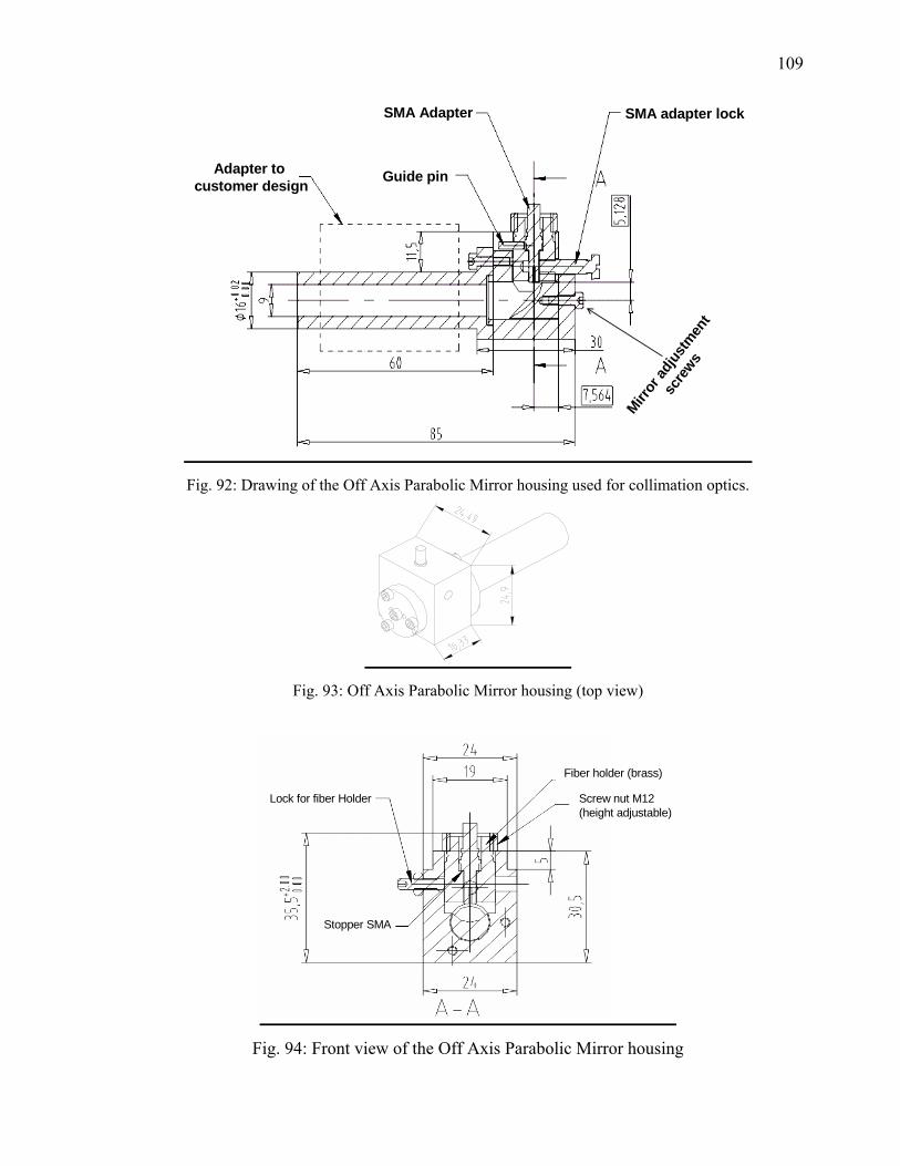
109
Adapter to customer design Guide pin
SMA adapter lockSMA Adapter
Mirror
adjus
tmen
t
scre
ws
Fig. 92: Drawing of the Off Axis Parabolic Mirror housing used for collimation optics.
Fig. 93: Off Axis Parabolic Mirror housing (top view)
Lock for fiber Holder
Stopper SMA
Fiber holder (brass)
Screw nut M12(height adjustable)
Fig. 94: Front view of the Off Axis Parabolic Mirror housing

110
Appendix-II Estimation of construction cost for the 2nd generation Multiwavelength Detector
Sl No. Item Description Part No. Supplier Cost
1
Mirror based Collimation
Optics with housing
Not Applicable
(a custom made item)
LFM Laboratory for Precision
Machining, University of
Bremen, Germany.
2600 €
2
Four channel Fiber feed
through (UV/Vis)
VAC-04-N-QMMJ-55-UVVIS-
50/125,940/1000-1,1.4-1,2.5
OZ Optics Limited, Ottawa,
Canada
1375 €
3
*USB series UV/Vis
Spectrometer with accessories
(including software)
USB 2G 558
USB 2E 3390
Ocean Optics BV, Duiven, the
Netherlands
2500 € (each)
4 Linear actuator (with
accessories: Power supply)
T-LA-28-SV Zaber Technologies Inc.
Columbia, Canada
700 €
5
Biconvex Quatrz lenses
(focal length: 12.5mm &
60mm)
G311-210-000 (f-60mm)
G311-204-000(f=12.5mm)
LINOS Photonics GmbH &
Co. KG, Goettingen, Germany
80 €
115€
6 High Power Xe- Flash lamp L-9456-12 Hamamatsu Photonics K K.,
Electron Tube Division, Japan
865 €
7 Power supply for the lamp 51672755 Conrad Electronic, Hirschau,
Germany
35 €
8 Electrical feed through HGP 3S 318 CLL SV
FFA 3S 318 CLAC 11
LEMO Elektronik GmbH,
München, Germany
35 €
35 €
9
LabView 7.1 Software
development environment
850670R-03
National Instruments
Corporation, Austin, Texas,
USA
1100 €
10 Heat sink modification
(preparative to a XL-I heat
sink)
Heat sink assembly, XLA2:
363404
Can Assembly, XLA: 363348
Beckman Coulter GmbH,
Krefeld, Germany
8000 €
11
Cost of the mechanical
components necessary
Leibniz-Institut für Molekulare
Pharmakologie, 13125 Berlin.
10800€
Total Cost 28240 €
Note: The above construction cost is on the basis of the detector adaptation to a preparative XL ultracentrifuge
(cost: ~50,000€). The cost for manufacturing the detector arm with the necessary modification in the XL-I
is just an estimate. The cost for constructing the reflection light gate is not included here as this was done at
BASF, Ludwigshafen. USB 2000 series spectrometers have been discontinued by the supplier, however,
UB4000 (cost: 2,500€) can be used instead (from the same supplier)

111
Appendix-III Alignment procedure for 2nd Generation optics
The alignment procedure consists of alignment of the mirror based collimator optics and then that of other optical components as described below:
1. Place a pinhole at the position of the 60mm biconvex lens (see fig. A, the position 6).
2. Fix a laser pointer at the slot where the collimation optics can be fitted (see fig. C).
3. Adjust the position of the three screws at the bottom of the plane mirror slot so that the emerging laser beam from the pointer hits the mid point in the pinhole (fig. C). These positions of the screws should be kept intact.
4. Remove the laser pointer from the collimator optics slot.
5. Place the mirror-based collimator optics in its slot.
6. Turn the cylindrical holder so that the white light beam hits the mid point in the pin hole (ref. fig. C)
7. Place the 60mm biconvex lens at its position (see fig. A)
8. Adjust the position of the 12.5mm biconvex lens (at position 7, in fig. A) in vertical direction to its highest intensity in the lamp spectra.
9. Make an optical resolution test (see sec. 6.4) and check if the position of the lens at position-7 is at optimum aligned position (compare with fig. B). The position of this lens should be adjusted in order to achieve the optimum optical resolution.
5.94 5.97 6.00 6.03 6.06 6.09 6.12 6.15 6.180
0
0
0
0
0
0
0
0
0
Radius Position
250 nm 300nm 400 nm 450nm
400nm, 90um
450nm, 73um
300nm, 83um
250nm,80um
XL A
50 100 150 200
0
200
400
600
800
1000
1200
1400
Inte
nsity
Distance moved by the step motor in µm
300nm 350nm 400nm 450nm 500nm 550nm
85um75um66um
44um48um
42um
Wavelength Resolution
AA BB
Mirror holder
Mirror
Plane mirror
Collim
ated light
Position of the screws for fine adjustment
Rotation of Holder
x y x-, y - m o vem en t o f the s tag e screw s
Sp ectro m ete r
CC
Fig.A (1) 50 micron fiber
UV/Vis, (2) Tip of the 50micron fiber, (3) Off axis parabolic mirror (4) Plane mirror (5)Iris Diaphragm(6) Focusing biconvex lens (60mm), (7) Focusing biconvex lens (12.5mm), (8) Spectrometer fitted in a x-,y- stage.
Fig. B Optics resolution test.
Intensity scan to be performed on a counter balance cell hole as the rotor spins at a speed of 3,000 rpm. Experimental conditions: step size: 1um, time/step: 100us.
Fig.C Schematic description of the alignment of different optical elements in the arm

112
Zusammenfassung
In der vorliegenden Arbeit wurde die Entwicklung neuer Detektoren für die
Analytische Ultrazentrifugation (AUZ) untersucht und vorangetrieben. Im Gegensatz zu
chromatgraphischen. Fraktionierungsmethoden werden Multidetektionssysteme bis heute
nicht in der AUZ eingesetzt.
Hier wird die Möglichkeit geprüft, bekannte spektroskopische sowie
Streumethoden simultan zur Probenanalyse in der AUZ einzusetzen mit dem Ziel,
simultan komplimentäre Informationen über die Probe zu erhalten. So wurde versucht,
Raman- und UV/VIS-Spektroskopie (letztere mit der Möglichkeit, das gesamte
Wellenlängenspektrum auszunutzen) und statische Lichtstreuung zu kombinieren, um das
Analytverhalten während des Ultrazentrifugationsexperimentes zu untersuchen. Es wurden
zum einen die Ramanspektroskopie als Detektionssystem für chemische Funktionalität in
der AUZ geprüft und zum anderen gezeigt, daß die statische Kleinwinkel Lichtstreuung
als direkter Molmassendetektor für den Einsatz in der AUZ geeignet erscheint. Zum
anderen wurde die Entwicklung eines Multi-Wellenlängen-UV/VIS-Detektors
abgeschlossen, um seine Eignung für den Einsatz in der AUZ und die damit verbundene
Möglichkeiten der schnelleren und umfassenderen Datenerzeugung gegenüber
kommerziellen Geräten zu zeigen.
Dieser Multiwellendetektor liefert anstelle eines Absorptionswertes für jede radiale
Position in der Messzelle direkt ein ganzes UV-Vis Spektrum und erzeugt eine
zusaetzliche Dimension der Messdaten, was die Möglichkeiten der Analyse von
komplexen Systemen mit multiplen Chromophoren, Teilchengrößenbestimmung über
Wellenlängenabhängigkeit der Trübung oder auch der Datenmittelung enorm vergrößert.
Desweiteren erlaubt der Detektor die Anwendung von Geschwindigkeitsprofilen zur
Analyse extrem polydisperser Systeme. Die Entwicklung des Detektors beruht auf einem
auf Linsen basierenden System mit modularem Aufbau. Dabei war die sorgfältige
Ausrichtung des optischen Systems ein essentieller Punkt, um seine Eignung zu
überprüfen zu können.

113
An einer Mischung von drei Kolloiden, Halbleiternanopartikeln sowie Proteinen
und deren Mischungen ist es hier gelungen, die erfolgreiche Entwicklung des UV/VIS-
Detektors zu demonstrieren: Die Daten konnten schneller und mit wesentlich mehr
Informationsgehalt, als auf allen kommerziellen Geräten generiert werden. Die
Sedimentationskoeffizientenverteilungen stimmen dabei mit denen aus herkömmlichen
Sedimentationsgeschwindigkeitsexperimenten überein, unterliegen jedoch nicht einer
signifikanten diffusionsbedingten Verbreiterung.
Es ist in dieser Arbeit somit gelungen, zum einen die Lichtstreuung als
aussichtsreiche Methode für ein Detektorsystem in der AUZ aufzuzeigen, und zum
anderen einen Multi-Wellenlängen-UV/VIS-Detektor zu entwickeln, der eine
Datenerzeugung von bislang noch nicht erreichter Schnelligkeit im dreidimensionalen
Raum ermöglicht.
114
Popular abstract
In this work approaches for new detection system development for an Analytical
Ultracentrifuge (AUC) were explored. Unlike its counterpart in chromatography
fractionation techniques, the use of a Multidetection system for AUC has not yet been
implemented to full extent despite its potential benefit. In this study we tried to couple
existing fundamental spectroscopic and scattering techniques that are used in day to day
science as tool for extracting analyte information. Trials were performed for adapting
Raman, Light scattering and UV/Vis (with possibility to work with the whole range of
wavelengths) to AUC. Conclusions were drawn for Raman and Light scattering to be a
possible detection system for AUC, while the development for a fast fiber optics based
multiwavelength detector was completed. The multiwavelength detector demonstrated the
capability of data generation matching the literature and reference measurement data and
faster data collection than that of the commercial instrument.
It became obvious that with the generation of data in 3-D space in the UV/Vis
detection system, the user can select the wavelength for the evaluation of experimental
results as the data set contains the whole range of information from UV/Vis wavelength.
The detector showed the data generation with much faster speed unlike the commercial
instruments. The advantage of fast data generation was exemplified with the evaluation of
data for a mixture of three colloids. These data were in conformity with measurement
results from normal radial experiments and without significant diffusion broadening. Thus
conclusions were drawn that with our designed Multiwavelength detector, meaningful data
in 3-D space can be collected with much faster speed of data generation.

115
Symbols di: particle diamtere
D: Diffusion coefficient
f: frictional coefficient
Fb: buoyant force
Ff: frictional force
Fs: gravitational force on a sedimenting particle
I: intensity of transmitted light
I0: intensity of incident light
m: mass of a particle
m0: mass of fluid that can be displaced by a particle
ω: angular velocity
r: distance of a particle from the axis of rotation
M: molar mass in g/mol
Mw: weight average molar mass
N: Avogadro’s number
v : partial specific volume
ρ0: density of the solvent
ρ2: density of sedimenting particle
η: solvent viscosity
R: gas constant
s: sedimentation coefficient
T: absolute temperature
λ: wavelength (e.g. for light)
116
Abbreviations APD: Avalanche Photodiode
AUC: Analytical Ultracentrifugation
BSA: Bovine Serum Albumin
BASF: Badische Anilin-und-Soda-Fabrik
CCD: Charge Coupled Device
DNA: DeoxyRibonucleic Acid
FTIR: Fourier Transform Infra Red spectroscopy
GC: Gas Chromatography
HTS: High Throughput Sampling
HPTLC: High Performance Thin Layer Chromatography
MS: Mass Spectrometry
NA: Numerical Aperture
Nd:YAG: Neodymium-Yttrium Aluminium garnet
OAP: Off Axis Parabolic Mirror.
PMT: Photo Multiplier Tube
RPM: Revolutions per Minute
RNA: Ribo Nucleic Acid
SDS: Sodium Dodecyl Sulphate
SMA: Sub Miniature version A
TLC: Thin Layer Chromatography
TTL: Transistor Transistor logic
TEM: Transmission Electron Microscopy
USB: Universal Serial Bus
UV: Ultraviolet

117
Acknowledgements I would like to take this opportunity to thank all the people who contributed to this work.
I am indebted to Prof. Dr. Markus Antonietti for financial support and allowing me to carry
out my doctoral work at MPI-KGF.
I am grateful to Dr. Helmut Cölfen for his never ending eagerness to help me at every front to
his maximum whenever it was necessary. Once again my special thanks to him for bearing
extra pain to read my thesis with valuable suggestions even from his hospital bed.
Many thanks to Andreas Kretzschmar for various mechanical design and construction of
mechanical parts.
Thanks to Henryk Pitas and Monika Scholz for the electronics work while building up the
instrumental setup
Special thanks to Akif Mehmeet Gülsun, Bilkent University, Ankara, Turkey for writing the
software for instrument control and data collection.
Thanks to Prof. Borries Demeler, University of Texas, San Antonio, Texas, USA for the data
viewer software.
Thanks to Frau Barth and Antje for their helpful assistance in the lab.
Thanks to Dr. Lars Börger, Dr. Wendel Wohlleben, Mr. Manfred Stadler, Mr. Thomas Meier,
BASF-AG, Ludwigshafen for various experimental components during laboratory work.
Thanks to Dr. Cecile Huin, Dr. Holger Strauss, Jong Seto and Dr. Miles Page for finding time to read my thesis.
My deep gratitude to all the members of MPI-KGF who made my life easier. To name a few
out of many, I owe my thanks to Nicole and Nadine for their warm friendliness and making
our office a memorable one. Also, our funny days with Özlem and Emre to get a relief from
the pain of Golm time.
Thanks to my parents and sisters and brother for their constant inspiration and the
conversations that I could stay aloof from homesickness.
Finally, I wish to thank Max Planck Society and BASF-AG for financial support.
118
References
1 Aurenkollektiv New Trends in Chemistry, Akademie-Verlag. Berlin 1982 2 Skoog D A, Leary J J; Principles of Instrumental analysis, 4th ed. Saunders: Fort Worth, 1992 3 Fung, E. N.; Chu, I.; Nomeir, A. A.; Rapid Commun. Mass Spectrom., 18 (2004) 2046 4 Lopez-Avila V, Hill H H; Anal Chem., 69 (1997) 289R 5Workman J. Jr., Koch Mel, Veltkamp D; Anal Chem., 77 (2005) 3789 6 Johnson K. J., Wright B. W. Jarman, K. H. Synovec, R. E.; J. Chromatogr., A 996 (2003) 141 7 LaTorre, A; Rigol, A.; Lacorte, S.; Barcelo, D.; J. Chromatogr., A 991 (2003) 205 8 Roussel, C.; Del Rio, A.; Pierrot-Sanders, J.; Piras, P.; Vanthuyne, N.; J. Chromatogr. A, 2004, 1037 (1-2),
3110328 9 Barreca, D.; Gasparotto, A; Tondello, E; Bruno, G.; Losurdo, M; J. Appl. Phys. 96 (2004) 1655 10 Hutter, K. J.; Lange, C.; Brewing Yest Fermentation Performance, 2nd Ed.; Blackwell Publishing Ltd.; Oxford,
UK., 2003; pg.169 11 Gurden, S.P.; Lage, E. M.; de Faria. C. G.; Joekes, I.; Ferreira, M. M. C.; J. Chemom. 17 (2003) 400 12 Andersson, M.; Svensson, o.; Folestad, S.; Josefson, M.; Wahlund, K.G.; Chemom. Intell. Lab. Syst. 75
(2005)1 13 Zhang, F,; Brueschweiler, R.; Chem. Phys. Chem. 5 (2004) 794 14 Ito, K.; Kato, T.; Ona, T.; Vib. Spectrosc 35 (2004) 159 15 Wildgoose, G. G.; Lawrence, N. S.; Leventis, H. C.; Li. J.; Jones, T. G. J.; Compton, R. G.; J. Mater. Chem. 15
(2005) 953 16 Kingston, H. Abstracts of the 35th Central Regional Meeting of the American Chemical Society, Pittsburg, PA,
Oct.19-22, 2003; p 47. 17 Hopke, P. K.; Anal Chim Acta 500 (2003) 185 18 Ertl, P.; Selzer, P.; Muehlabacher, J.; Drg Discovery Today: BIOSILICO 2 (2004) 201 19 Saundrs, K. C. Drug Discovery Today; Technol. 1(2004) 373 20 Cadapakam JV, Zelechonok Y; Anal Chem. 75 (2003) 3484 21 Gilar M, Olivova P, Daly AE, Gebler JC; Anal Chem. 77 (2005) 6426 22 Roger P, Axelos MAV, Colonna P; Macromolecules, 33 (2000) 2446 23 Osterloh K, Borchert HH, Kroll C; Detector: ESR for Chrmatography, Encyclopedia of separation science,
Vol. 2, Academic Press (2000) 24 Svedberg T, Rinde H; J. Am. Chem. Soc. 45 (1924) 2 25 Svedberg T, Pedersen K O; The Ultracentrifuge, Claredon Press, Oxford (1940)
26 Balbo A, Minor KH, Velikovsky CA, Mariuzza RA, Peterson CB, Schuck P; Proc. Natl Acad Sci USA 102 (2005) 81 27 http://www.analyticalultracentrifugation.com 28 http://www.analyticalultracentrifugation.com/sedphat/sedphat.htm 29 http://www.ultrascan.uthscsa.edu 30 http://www.bbri.org/faculty/stafford/AUCRL.html
119
31 Lloyd P.H. Optical Methods In Ultracentrifugation, Electrophoresis, and Diffusion; Clarendon Press, Oxford
1974. 32 Lamm O, Ark. Math. Astron. Fysik 21B, Nr. 2, (1929) 1 33 Ralston G; Introduction to Analytical Ultracentrifugation, Beckman Coulter Inc.Fullerton, US. 34 Lee J. C., S Rajendran; Studies of macromolecular interaction by sedimentation velocity, in T M Schuster and
Laue T M; Modern analytical ultracentrifugation, Birkhäuser, Boston, Basel, Berlin(1994) 138. 35 Goldberg R J; J. Phys. Chem. 57 (1953) 194 36 Van Holde KE, Weischet WO; Biopolymers 17 (1978) 1387 37 Demeler B, Saber H, Hansen JC; Biophys 72 (1997) 397 38 Muramatsu N, Minton A. P., Anal Biochem. 168 (1988) 345 39 Stafford W. F., ‘Method for obtaining sedimentation coefficient distributions’ in Harding S. E., Rowe A. J.,
Horton J. C., Analytical ultracentrifugation in biochemistry and polymer science, The royal society of chemistry, Cambridge (1992) 359.
40 Yaphantis D.A., Biophys J 45 (1984) 324a 41 Stafford W. F., Anal Biochem. 203 (1992) 295 42 Van Holde K.E., Baldwin R. L., J. Phys. Chem. 62 (1958) 734 43 Yaphantis D.A., Ann N. Y. Acad Sci. 88 (1960) 586 44 Mächtle. W, ‘Analysis of polymer dispersions with an eight cell AUC multiplexer: High resolution particle
size distribution and density gradient tecniques’ in Harding SE, Rowe AJ, Horton JC, Analytical Ultracentrifugation in biochemistry and polymer science, The royal society of chemistry, Cambridge (1992) 147.
45 Budd PM; Progr. Colloid Polym Sci. 94 (1994) 107 46 Vinograd J, Lebowitz J, Radloff R, Watson R, Laipis P Proc Natl. Acad. Sci, USA 53 (1965) 1104 47 Lebowitz J, Teale M, Schuck P, Biochem. Soc. Trans. 26 (1998) 745 48 http://www.analyticalultracentrifugation.com/sedfit_help_analytical_zone_centrifugation.htm 49 Giebeler R (1992) The Optima XL-A: A New Analytical Ultracentrifuge with a Novel Precision Absorption
Optical System, in: Harding SE et al (ed) Analytical Ultracentrifugation in Biochemistry and Polymer Science, Royal Society of Chemistry, Cambridge, 16
50 Schachman HK, Ultracentrifugation in Biochemistry, Academic Press (1959) 51 Flossdorf J; Makromol Chem 181 (1980) 715 52 Laue TM, PhD Dissertation, 1981 University of Connecticut, Storrs CT 53 Laue TM, On-Line Data Acquisition and Analysis from the Rayleigh Interferometer in Harding SE, Rowe AJ,
Horton JC, Analytical Ultracentrifugation in biochemistry and polymer science, The royal society of chemistry, Cambridge (1992) 147
54 Rowe AJ, Jones SW, Thomas DG, Harding SE; Method for offline analysis of sedimentation velocity and
sedimentation equilibrium patterns, in Harding SE, Rowe AJ, Horton JC, Analytical Ultracentrifugation in biochemistry and polymer science, The royal society of chemistry, Cambridge (1992) 147.
55 Harding SE, Rowe AJ; Optics and Lasers in Engineering; 8 (1988) 83 56 Flossdorf J, Schilling H, Schindler KP; Makromol Chem 179 (1978) 1617 57 Scheibling G, J Chim Phys; 47 (1950) 688
120
58 Lavrenko P, Lavrenko V, Tsvetkov V, Prog. Colloid Polym Sci. 113 (1999) 14 59 Lebdev AA; Tr Gos Opt Inst Leningr 5 (1931) 53 60 “Beobachtungen nach einer neuen optischen Methode”, Toeppler. A; Bonn 1864 61 Tanner CC; Trans. Faraday Soc. 23 (1927) 75 62 Lamm O; Nova Acta R. Soc. Sci. Upsal. 10, Nt. 6, 1937 63 Instrument Manual of SPINCO Model E Analytical Ultracentrifuge, Beckman Instruments, Inc. Spinco
Division, Palo Alto, California. 64 Cölfen H, Borchard W; Ultrasensitive Schlieren Optical System Biomedical Diagnostic Instrumentation, Proc.
SPIE 2136 (1994) 65 Mächtle. W, Börger L; Analytical Ultracentrifugation of Polymers and Nanoparticles, Springer Laboratory
Manuals in Polymer Science (2006). 66 Mächtle. W: Progr. Colloid. Inte. Sci. 113 (1999) 1 67 Börger L, Lechner MD, Stadler M; Prog. Colloid Polym Sci 127 (2004) 19 68 Klodwig U, Mächtle, Colloid Polym. Sci 267(1989) 1117 69 Clewlow AC, Errington N, Rowe AJ; Eur. Biophys. J. 25 (1997) 311 70 Cölfen H, Borchard W; 94 (1994) 90 71 MacGregor I. K., Anderson A. L., Laue T. M.; Biophysical Chemsitry 108 (2004) 165-185. 72 Schmidt B, Riesner D, A Fluorescence Detection system for Analytical Ultracentrifuge and its Application to
Proteins, Nucleic Acis, Viroids and Viruses in Harding SE, Rowe AJ, Horton JC, Analytical Ultracentrifugation in biochemistry and polymer science, The royal society of chemistry, Cambridge (1992)
73 Cantow HJ; Makromol Chem 70 (1964)130 74 Mächtle. W; Makromol Chem 185 (1984) 1025 75 Scholtan W, Lange H; Kolloid Z Z Polym 250 (1972) 782 76 Mächtle W, Börger L; Analytical Ultracentrifugation, Instrumentation, in Analytical ultracentrifugation of
Polymers and Nanoparticles, Springer (2005) 77 Svedberg T,Pedersen KO; The Ultracentrifuge, Clarendon Press, Oxford (1940) 78 Cölfen H, Völkel A.; Progr. Colloid Polym Sci 2004 (127) 31-47 79 Liu. J, Shire S. J.; J. Pharm Sci. Vol. 88, No. 12. 80 Shire S. J.; Modern Analytical Ultracentrifugation, Todd M Schuster, Thomas Laue, Birkhäuser 81 Ralston G.; Introduction to Analytical Ultracentrifugation, Beckman Instruments Inc, California. 82 Analytical Ultracentrifugation Techniques and Methods, Edited by Scott DJ, Harding SE, Rowe AJ., RSC
Publishing (2005) 83 Analytical Ultracentrifugation of Polymers and Nanoparticles by Mächtle W, Börger L, Springer (2005) 84 Analytical Ultracentrifugation in biochemistry and polymer science, edited by Harding SE, Rowe AJ, Horton
JC, The royal society of chemistry, Cambridge (1992) 85 Svedberg T, Rinde H, J. Am. Chem Soc. 46 (1924) 2677 86 Rinde H, The distribution of the sizes of particles in gold sols, PhD thesis Upasala (1928) 87 Nichols J B, Physics 1 (1931) 254 88 Nichols J B, Kramer E O, Bailey E D, J. Phys. Chem., 36 (1932) 326
121
89 Rapport DH, Vogel W, Cölfen H, Schlögl R; J. Phys. Chem. B 101 (1997) 136 90 Müller HG, Herrmann F; Progr. Colloid Polym. Sci. 107 (1997) 136 91 Mächtle. W; Biophys. J. 76 (1999) 1080 92 Cölfen H, Pauk T, Colloid Polym Sci. 275 (1997) 136 93 Richards, J. P.; Stickelmeyer, M. P.; Flora, D. B.; Chance, R. E.; Frank, B. H..; Defelippis, M. R.; Pharm. Res.
1998 (15) 1434-1441 94 Verley, P. G.; Brown, A. J.; Dawkes, H. C.; Burns, N. R.; Eur. Biophys. J. 1997, (25), 437-443 95 Philo, J. S.; Aoki, K. H.; Arakawa, T.; Narhi, L. O.; Wen, J.; Biochemistry 1996, (35), 1681-1691. 96 Pennica, D.; Kohr, W. J.; Weber, Fendly B. M.; Shire, S. J.; Raab, H. E.; Borchardt, P. E.; Lweis, M.; Goedel,
D. V.; Biochemistry 1992 (31) 1134-1141 97 Pennica, D.; Lam, V. T.; Weber. R. F.; Kohr, W. J.; Basa, L. J.; Spellman, M. W.; Ashkenazi. A; Shire, S. J.;
Goedel, D. V.; Biochemistry 1993 (32) 3131-3138 98 Cunningham, B. C.; Mulkerrin, M. G.; Wells J. A.; Science, 1991, 253, 545-548. 99 Liu, J.; Laue, T. M.; Choi, H. U.; Tang, L. H.; Rosenberg, L.; J. Biol. Chem. 1994 (269) 28366-28373. 100 Winfield, P.; Graber, P.; Moonen, P.; Craig, S.; Pain, R. H.; Eur. J. Biochem. 1988, (173), 65-72 101 Van Holde, K. E.; Weischet, W.; Biopolymers 1978 (17) 1387-1403 102 Demeler, B.; Saber, H.; Hansen, J. C.; Biophys. J. 1997 (72) 397-407 103 Hansen. J. C.; Lebowitz, J.; Demeler, B.; Biochemistry 1994 (33) 13155-13163 104 Hansen, J. C.; Ausio, J; Stanik, V. H.; van Holde K. E.; Biochemistry 1989 (28) 9129-9136 105 Gill, S. C.; Yager, T. D.; von Hippel, P. H.; J. Mol. Biol. 1991 (220) 325-333 106 Stafford, W. F. I.; Curr. Opin Biotechnol. 1997, (8) 14-24 107 Stafford, W. F.; Anal. Biochem. 1992 (72) 397-407 108 Liu. J.; Ruppel, J.; Shire, S. J.; Pharm. Res. 1997 (14) 1388-1393 109 Laue, T. M.; Johnson, A. E.; Esmon, C. T.; Yphantis, D. A.; Biochemistry 1984 (23) 1339-1348 110 Kim, S. J.; Tsukiyama, T.; Lewis, M. S.; Wu, C.; Protein Sci. 1994 (3) 1040-1051 111 Behlke J, Eur Biophys. J. 25 (1997) 319 112 Behlke J, Ristau O; Eur Biophys. J. 25 (1997) 325 113 Harding SE; Sedimentation Analysis of Polysaccharides, in: Harding SE et al (ed) Analytical
Ultracentrifugation in Biochemistry and Polymer Science, Royal Society of Chemistry, Cambridge, 16 114 Mächtle W; Progr. Colloid Polym. Sci 86 (1991) 111 115 Malacara D, Malacara Z; Handbook of Optical Design, 2nd Ed. Marcel Dekker, New York, Basel. 116 Kisters D, Borchard W; Progr. Colloid Polym Sci 1994, 113, 10. 117 Börger L, Lechner MD, Stadler M; Progr. Colloid Polym Sci 2004, 127, 19 118 Mächtle W, Progr. Colloid Polym Sci; 1999, 113, 1 119 Rockholt DL, Royce CR, Richards; Biophys Chem 1976, 5, 55 120 Kim J E, McCamant D W, Zhu L, Mathies R A; J Phys. Chem B 2001, 105, 1240-1249. 121 Kochendoerfer G. G., Lin S.W., Sakmar T.P., Mathies R. A.; Trends Biochem. Sci.1999, 24, 300–305. 122 Wu Y J, Xu Y Z, Zhao Y, Wang D J, Weng S F, Wu J G, Xu D F; SPECTROSCOPY AND SPECTRAL ANALYSIS

122
25, 9, 1408-1411, SEP 2005
123 DeGraff. B A, Hennip M, Jones J M, Salter C, Schaertel S A, Chem. Educator 2002, 7, 15-18. 124 www.chromexinc.com/ (accessed in 2003 Nov.) 125 http://www.kosi.com/ (accessed in 2003 Nov.) 126 http://www.jyinc.com/ (accessed in 2003 Nov.) 127 Liu T, Chu Benjamin; Encyclopedia of Surface and Colloid Science; Marcel Dekker, Inc. 2002. 128 Chu B. Laser Light-Scattering, 2nd Ed.; Academic Press:New York, 1991. 129 Schuck P; Prog. Colloid & Polym. Sc. (1994) 94 1 130 Servillo L, Brewer HB, Osborne JC; Biophys Chem (1981) 13 29 131 Lakatos S, Minton P; J Biol Chem. (1991) 226 18707 132 Cantow HJ (1964) Makromol. Chem. 70: 130 133 Scholtan W, Lange H (1972) Kolloid Z Z Polym. 250: 782 134 Müller HG (1989) Colloid Polym. Sci. 267: 1113 135 Flossdorf J (1980) Makromol. Chem. 181: 715 136 Flossdorf J, Schillig H (1979); Feinwerktechnik Messtechnik 93: 87 137 Voelker P (1995) Progr Colloid Polym Sci 99: 162 138 Vistica J, Dam J, Balbo A, Yikilmaz E, Mariuzza RA, Rouault TA, Schuck P (2004) Anal Biochem 326: 234
139 Gledhill RJ (1962) J Phys Chem 66: 458 140 Bateman JB, Weneck EJ, Eshler DC (1959) J Colloid Sci 14: 308 141 Heller W, Bhatnagar HL, Nakagaki M (1962) J Chem Phys 36: 1163 142 Hosono M, Sugii S, Kusudo O, Tsuji W (1973) Bull Inst Chem Res, Kyoto Univ 51: 104 143 http://oceanoptics.com/technical/engineering/USB2000%20OEM%20Data%20Sheet.pdf 144 http://oceanoptics.com/technical/engineering/OEM%20Data%20Sheet%20--%20HR4000.pdf 145 www.lot-oriel.com/ccd 146 http://usa.hamamatsu.com/en/products/electron-tube-division/light-sources/xenon-flash-lamps.php. 147 Instruction Manual for Xe Flash Lamp Module (L-9455, L-9456 series), Hamamatsu PhotonicsK. K., Electron
Tube Division, Japan. 148 Niederberger M, Garnweitner G, Krumeich f; Nesper r, Cölfen H, Antonietti M (2004) Chem. Mater.4, 16,
1202. 149 dantecdynamic.com