Matematisk modellering og dataanalyse af dynamiske ... · Matematisk modellering og dataanalyse af...
9
university of copenhagen Faculty of Science Matematisk modellering og dataanalyse af dynamiske processer i biologi Susanne Ditlevsen Institut for Matematiske Fag Københavns Universitet Mød Matematik p˚ a KU 13. november 2014 Slide 1/34 university of copenhagen mathematical sciences Matematisk og statistisk modellering Matematisk og statistisk modellering benytter matematik og statistik til at • beskrive fænomener i den virkelige verden • undersøge vigtige spørgsm˚ al om den observerede verden • forklare fænomener i den virkelige verden • teste ideer • lave forudsigelser om den virkelige verden Slide 2/34 — Susanne Ditlevsen — Statistik og matematisk modellering — 13. november 2014 university of copenhagen mathematical sciences Matematisk og statistisk modellering Den virkelige verden kan være • fysik • fysiologi • biologi • økologi • kemi • økonomi • sport • ··· Slide 3/34 — Susanne Ditlevsen — Statistik og matematisk modellering — 13. november 2014 university of copenhagen mathematical sciences Matematisk og statistisk modellering Eksempler p˚ a spørgsm˚ al vi kan belyse med matematiske modeller • Hvordan spiller glukose, insulin og fedt sammen i den menneskelige fysiologi? • Med hvilke tidsintervaller skal lyskurvene skifte for at trafikken flyder bedst muligt? • Hvad er den bedste investeringsstrategi? • Er den globale opvarmning (delvist) menneskeskabt? • Hvordan bliver vejret i morgen? Slide 4/34 — Susanne Ditlevsen — Statistik og matematisk modellering — 13. november 2014
Transcript of Matematisk modellering og dataanalyse af dynamiske ... · Matematisk modellering og dataanalyse af...

un i v er s i ty of copenhagen
Faculty of Science
Matematisk modellering og dataanalyse af
dynamiske processer i biologi
Susanne DitlevsenInstitut for Matematiske FagKøbenhavns Universitet
Mød Matematik pa KU
13. november 2014
Slide 1/34
un i ver s i ty of copenhagen mathemat i ca l s c i ence s
Matematisk og statistisk modellering
Matematisk og statistisk modellering benyttermatematik og statistik til at
• beskrive fænomener i den virkelige verden
• undersøge vigtige spørgsmal om den observeredeverden
• forklare fænomener i den virkelige verden
• teste ideer
• lave forudsigelser om den virkelige verden
Slide 2/34 — Susanne Ditlevsen — Statistik og matematisk modellering — 13. november 2014
un i v er s i ty of copenhagen mathemat i ca l s c i ence s
Matematisk og statistisk modellering
Den virkelige verden kan være
• fysik
• fysiologi
• biologi
• økologi
• kemi
• økonomi
• sport
• · · ·
Slide 3/34 — Susanne Ditlevsen — Statistik og matematisk modellering — 13. november 2014
un i ver s i ty of copenhagen mathemat i ca l s c i ence s
Matematisk og statistisk modellering
Eksempler pa spørgsmal vi kan belyse med matematiskemodeller
• Hvordan spiller glukose, insulin og fedt sammen iden menneskelige fysiologi?
• Med hvilke tidsintervaller skal lyskurvene skifte forat trafikken flyder bedst muligt?
• Hvad er den bedste investeringsstrategi?
• Er den globale opvarmning (delvist) menneskeskabt?
• Hvordan bliver vejret i morgen?
Slide 4/34 — Susanne Ditlevsen — Statistik og matematisk modellering — 13. november 2014
un i v er s i ty of copenhagen mathemat i ca l s c i ence s
Matematisk og statistisk modellering
Udfordring:
“...not to produce the most comprehensivedescriptive model”
men
“to produce the simplest possible model thatincorporates the major features of the
phenomenon of interest”
Howard Emmons
All models are wrong but some are useful.
George E. P. BoxSlide 5/34 — Susanne Ditlevsen — Statistik og matematisk modellering — 13. november 2014
un i ver s i ty of copenhagen mathemat i ca l s c i ence s
Matematisk og statistisk modellering
• Eksperimentelle videnskabsfolk er rigtig gode tilstudere sma komponenter fra den virkelige verden
• Den virkelige verden er ikke-lineær, og det er etmeget svært puslespil at fa komponenterne satsammen til et hele
• Matematisk modellering kan netop gøre det!
• Ideelt set vil kombinationen af eksperimenter ogmodellering hjælpe til en fuldstændig forstaelse afdet fænomen, man studerer
Slide 6/34 — Susanne Ditlevsen — Statistik og matematisk modellering — 13. november 2014
un i v er s i ty of copenhagen mathemat i ca l s c i ence s
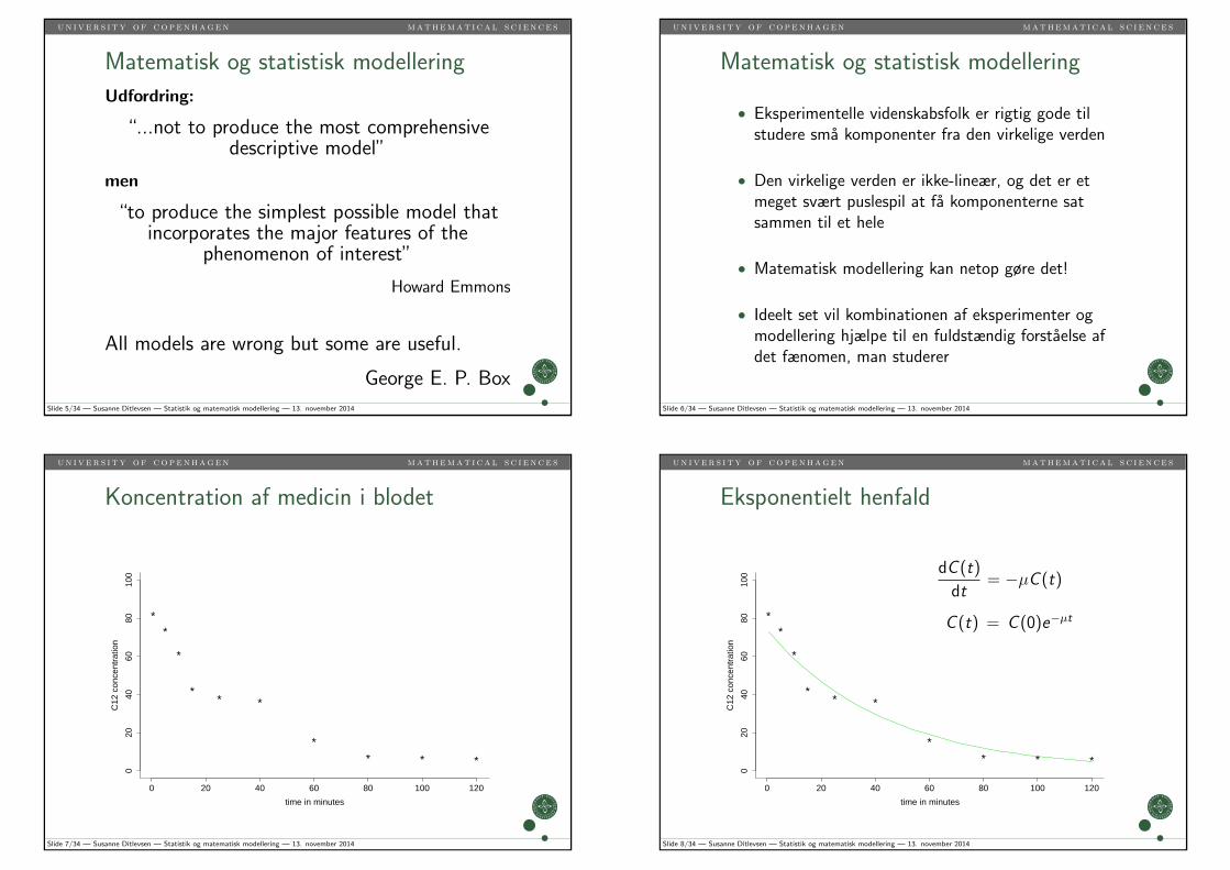
Koncentration af medicin i blodet
**
*
** *
** * *
0 20 40 60 80 100 120
020
4060
8010
0
time in minutes
C12
con
cent
ratio
n
Slide 7/34 — Susanne Ditlevsen — Statistik og matematisk modellering — 13. november 2014
un i ver s i ty of copenhagen mathemat i ca l s c i ence s
Eksponentielt henfald
dC (t)
dt= −µC (t)
C (t) = C (0)e−µt**
*
** *
** * *
0 20 40 60 80 100 120
020
4060
8010
0
time in minutes
C12
con
cent
ratio
n
Slide 8/34 — Susanne Ditlevsen — Statistik og matematisk modellering — 13. november 2014
un i v er s i ty of copenhagen mathemat i ca l s c i ence s
Eksponentielt henfald med støj
dC (t) = −µC (t)dt + σC (t)dW (t)
C (t) = C (0) exp(−(µ + 1
2σ2)t + σW (t)
)*
*
*
** *
** * *
0 20 40 60 80 100 120
020
4060
8010
0
time in minutes
C12
con
cent
ratio
n
Slide 9/34 — Susanne Ditlevsen — Statistik og matematisk modellering — 13. november 2014
un i ver s i ty of copenhagen mathemat i ca l s c i ence s
Forskellige udfaldsstier
dC (t) = −µC (t)dt + σC (t)dW (t)
C (t) = C (0) exp(−(µ + 1
2σ2)t + σW (t)
)*
*
*
** *
** * *
0 20 40 60 80 100 120
020
4060
8010
0
time in minutes
C12
con
cent
ratio
n
Slide 10/34 — Susanne Ditlevsen — Statistik og matematisk modellering — 13. november 2014
un i v er s i ty of copenhagen mathemat i ca l s c i ence s
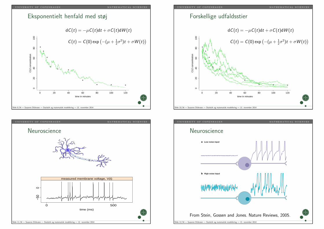
Neuroscience
time (ms)
−50
0
0 500
measured membrane voltage, V(t)
Slide 11/34 — Susanne Ditlevsen — Statistik og matematisk modellering — 13. november 2014
un i ver s i ty of copenhagen mathemat i ca l s c i ence s
Neuroscience
a Low noise input
b High noise input
REFRACTORY PERIODThe period of time after a spike when a neuron is unable or less able to fire another spike.
represent 2 bits (or 22 = 4 choices). Therefore, if the REFRACTORY PERIOD of a neuron is less than 1 ms, it could transmit more than 1,000 (103) bits of information in 1 s in a sensory process. However, if different stimulus intensities are presented to a human observer (with 1012 neurons), and the observer assigns a numerical score to each stimulus presentation, approximately seven categories can be reliably discriminated8. When more choices are presented, observers make errors and the information calculated from information theory is still roughly equivalent to seven categories. So, although the system has the potential to transmit 103 × 1012 = 1015 bits in 1 s, conscious perception can provide less than 3 bits (or 23 = 8 categories) of information about stimulus intensities in a range of sensory systems.
The rate code. This large discrepancy was soon resolved experimentally and theoretically. As mentioned above, Lord Adrian proposed the rate code in which the inten-sity of a signal is represented as the number of spikes from a single neuron or a population of neurons over a period of time. The rate is obtained by dividing the number of spikes by the time period. In other words, signals in the sequence 100 (spike, no spike, no spike) over a period of 3 ms would be interpreted not as the binary representation of the number 4, but as a rate of 1 spike in 3 ms, which corresponds to 333 spikes in 1 s. This code would be indistinguishable from the sequences 010 and 001. In such a rate code, the total number of spikes over a period of time is the determin-ing factor, rather than the order or timing of spikes. Variability in the inter-spike intervals and, therefore,
in the total number of spikes in 1 s, for example, would limit the amount of sensory information that neurons transmit.
If the input to a neuron has little noise (FIG. 1a), the neuron will depolarize to the threshold at a steady rate and the number or rate of spikes over a period of time will be reproducible. With a noisy input (FIG. 1b), the spikes will be generated with variable intervals and the rate of spikes over time will also vary. Values of infor-mation capacity of 2 or 3 bits have been calculated for single neurons in sensory systems, using rate coding to distinguish the levels of response to steady inputs over 1 s REF. 9,10. In fact, Talbot and colleagues11 directly calculated the information contained in the firing of sensory receptors of a monkey to a flutter vibration applied to the skin and found that it agreed with the information from human observers respond-ing to the same sensory stimulus. This agreement between responses in monkey sensory receptors and human experiments was encouraging, but several questions remained.
The problems with the rate code. First, as most sensory stimuli activate many receptors, a human observer should be able to use the larger number of nerve impulses from the population of sensory neurons to distinguish more categories. In other words, if a whole population of neurons is active, and each neuron sends 2 or 3 bits to the brain in 1 s, why is human perception limited to less than 3 bits? Is the agreement between the calculated values of information capacity for single neurons and the human observer merely fortuitous? The answer to the latter question is probably yes. With a rate code, the number of bits of information increases according to the square root of the number of impulses, regardless of whether the impulses come from a single neuron or a population of neurons10. Therefore, 100 neurons would transmit 10 times the information of a single neuron. If the brain uses 100 neurons to perceive different categories, we would expect ~20–30 bits of information to be transmitted in 1 s, which predicts more than a million possible perceptual categories. The information contained in the responses from populations of cells must under-lie the ability to recognize faces, as mentioned above. However, some information might be lost in synaptic relays or in memory storage in the brain. Conceivably, this loss might cancel out the extra information that is contained in the population of sensory neurons in the particular laboratory experiments quoted above and leave 2 or 3 bits (or 7 categories). These issues still need to be rigorously tested experimentally.
Second, if variability in inter-spike intervals creates noise that limits information flow in sensory systems, why have sensory neurons not evolved to reduce this variability? As discussed below, in relation to temporal codes, neurons do fire spikes at precise times in some sensory systems. In others, the receptors are operating close to physical limits that introduce variability. For example, in the visual system, photons arrive randomly in time and, under some conditions, a single photon
Figure 1 | Variability in neuronal firing. a | With a relatively steady depolarizing input current (low noise), spikes are generated at a regular rate. b | With higher noise, which could arise from a combination of excitatory and inhibitory postsynaptic potentials, the variability in firing rate is much higher, even though the mean firing rate might be similar. These data were simulated from a neural model with a leaky integrator and a fixed threshold82. The range in variability shown is typical of many neurons.
390 | MAY 2005 | VOLUME 6 www.nature.com/reviews/neuro
R E V I E W S
© 2005 Nature Publishing Group
From Stein, Gossen and Jones. Nature Reviews, 2005.
Slide 12/34 — Susanne Ditlevsen — Statistik og matematisk modellering — 13. november 2014
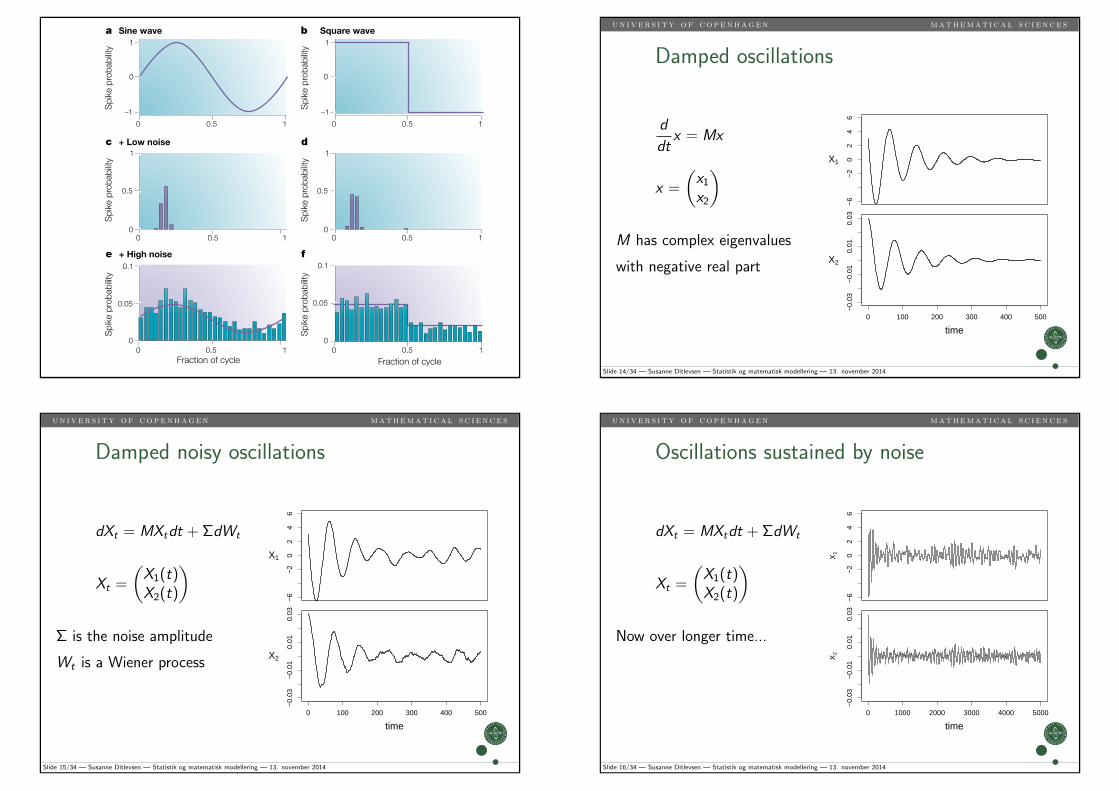
0 0.5 1
–1
0
1
a Sine wave b
d
f
0 0.5 1
–1
0
1
Square wave
0 0.5 10
0.5
1c + Low noise
Spi
ke p
roba
bilit
yS
pike
pro
babi
lity
Spi
ke p
roba
bilit
y
Spi
ke p
roba
bilit
yS
pike
pro
babi
lity
Spi
ke p
roba
bilit
y
0 0.5 10
0.5
1
0 0.5 10
0.05
0.1
e + High noise
Fraction of cycle0 0.5 1
0
0.05
0.1
Fraction of cycle
STOCHASTIC PROCESSA random sequence of events; if the probability of occurrence of the events is the same with each small increment of time, it is referred to as a Poisson process.
BANDWIDTHThe range between the lowest and highest frequencies of oscillation that produce a response.
ENTRAINEDThe state in which one signal is linked to the repetitive behaviour of another.
HARMONICSIntegral multiples of the fundamental frequency.
can lead to perception12. The variability in the timing of spikes might be related to the irregular arrival of photons. Similarly, Brownian motion affects hair cells in the auditory system13,14. Therefore, the presence of variability in sensory systems might be an inevitable consequence of exquisitely responsive sensors. Furthermore, during synaptic transmission through sensory and central synapses, the effects of individual excitatory postsynaptic potentials (EPSPs) are relatively large compared with those of individual ions in the con-stant currents that were considered in FIG. 1a REF. 15. If the generation of EPSPs is a random or STOCHASTIC
PROCESS, variability will be introduced in the time that is taken to reach the threshold for spike generation16,17. According to this view, the response variability of neu-rons in the CNS is a property of synaptic connections rather than the neurons themselves18. Below, we discuss evidence from the work of Mainen and Sejnowski, and others on the advantages of signal variability, which shows that the generation of EPSPs is not random and that their large size can be used to preserve timing information across synapses.
Finally, are these low rates of information transfer a consequence of studying steady signals? The answer to this question is probably also yes. The most important biological signals are changes in environmental param-eters, such as light intensity. Sensory neurons respond to changing signals over a range of frequencies BAND
WIDTH and can only signal information in their normal
working range. The bandwidth limits the maximum information capacity, but much more information can be transmitted with changing, rather than steady, sig-nals. Experimental attempts to measure information capacity with broad-bandwidth random inputs have yielded approximate values of 1 bit per spike19,20. If neu-rons fire tens or even hundreds of spikes per second, then tens or hundreds of bits per second are also pos-sible, rather than only three with steady signals. Indeed, with rapidly varying signals, rates must be measured over small time intervals, so the distinction between rate and temporal codes breaks down. A more mean-ingful measure is the accuracy in the timing of spikes in individual neurons in response to the changing stimulus, which can be of the order of milliseconds in cortical neurons and tenths of a millisecond in some sensory neurons21,22.
Advantages of signal variability. Recent studies indi-cate that variability might also offer distinct advan-tages. Noise could enhance sensitivity to weak signals, a pheno menon that is known as ‘stochastic reso-nance’23–25. As sensory signals are variable, Knill and Pouget26 suggested that the brain might also code sen-sory information probabilistically and use the method of Bayesian inference. With this approach, the decision processes in the brain could deduce the best choice by combining previous experience with the probabilistic sensory signal27.
An example of the potential advantages of signal variability is presented in FIG. 2. If a sine wave with a period of 30 ms is applied to a muscle or a cutaneous receptor (FIG. 2a), the neuron becomes ENTRAINED to the stimulus, with one spike for each sinusoidal cycle. This gives information about the period, but not the form of the stimulus. A square wave with the same period (FIG. 2b) produces a similar train of spikes. Variability in the individual neurons can prevent this entrain-ment28,29. With little noise, using the neural model of FIG. 1a, the responses to the sine wave would occur near a specific point in the cycle and would be indistinguish-able for a sine or square wave (FIG. 2c,d). With more noise, as typically occurs in many neurons, the inter-spike intervals are more variable and the cycle histograms assume distinct shapes. The average responses to the sine and the square waves now match the waveforms of the input signals (FIG. 2e,f).
The problem of entrainment becomes greater the higher the frequency of the applied signals. Therefore, it is most acute in the auditory system, as this receives tones with frequencies of several kiloHertz, which is higher than in other sensory systems. However, a 400-Hz tone on a violin can be distinguished from a similar tone on an oboe. Although the fundamental frequency is the same, the HARMONICS that are produced by an oboe and a violin at 800 Hz and higher frequen-cies have different strengths. As the firing of cochlear neurons is close that expected for a random or Poisson process30, the resulting high degree of variability ensures that the different harmonic structures of the signals from the violin and oboe produce a different average
Figure 2 | Noise can be beneficial to the faithful transmission of high-frequency inputs. When a sine wave (a) or square wave (b) with a period of 30 ms is added as an input to the low-noise neural model shown in FIG. 1a, the input entrains the firing of the neural model so that it generates one spike per cycle at a relatively fixed phase (c and d) and the shape of the input is lost. Adding the same inputs to the high-noise model shown in FIG. 1b produces spikes at all phases and the probability follows the shape of the input (e and f).
NATURE REVIEWS | NEUROSCIENCE VOLUME 6 | MAY 2005 | 391
R E V I E W S
© 2005 Nature Publishing Group
un i ver s i ty of copenhagen mathemat i ca l s c i ence s
Damped oscillations
d
dtx = Mx
x =
(x1x2
)
M has complex eigenvalues
with negative real part
−6
−2
02
46
X1
0 100 200 300 400 500
−0.
03−
0.01
0.01
0.03
time[plotseq]time
X2
Slide 14/34 — Susanne Ditlevsen — Statistik og matematisk modellering — 13. november 2014
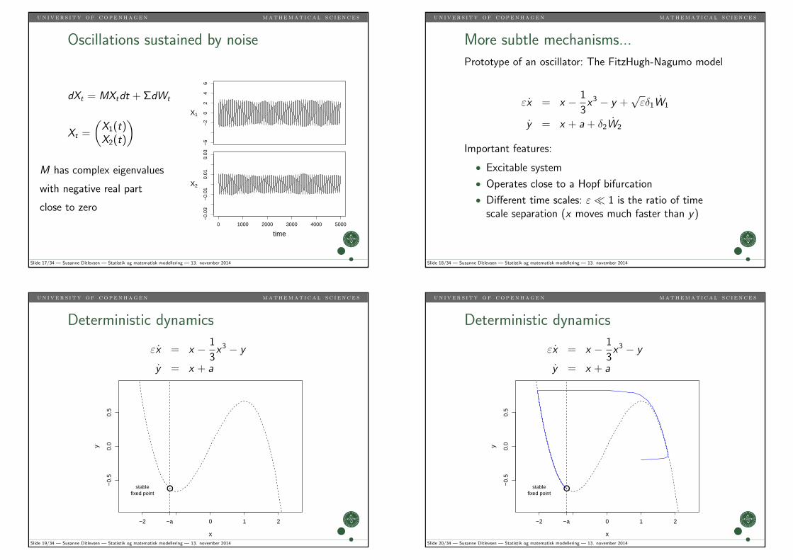
un i v er s i ty of copenhagen mathemat i ca l s c i ence s
Damped noisy oscillations
dXt = MXtdt + ΣdWt
Xt =
(X1(t)X2(t)
)
Σ is the noise amplitude
Wt is a Wiener process
−6
−2
02
46
X1
0 100 200 300 400 500
−0.
03−
0.01
0.01
0.03
time[plotseq]time
X2
Slide 15/34 — Susanne Ditlevsen — Statistik og matematisk modellering — 13. november 2014
un i ver s i ty of copenhagen mathemat i ca l s c i ence s
Oscillations sustained by noise
dXt = MXtdt + ΣdWt
Xt =
(X1(t)X2(t)
)
Now over longer time...
X1
−6
−2
02
46
0 1000 2000 3000 4000 5000
−0.
03−
0.01
0.01
0.03
time[plotseq]
X2
time
Slide 16/34 — Susanne Ditlevsen — Statistik og matematisk modellering — 13. november 2014
un i v er s i ty of copenhagen mathemat i ca l s c i ence s
Oscillations sustained by noise
dXt = MXtdt + ΣdWt
Xt =
(X1(t)X2(t)
)
M has complex eigenvalues
with negative real part
close to zero−
6−
20
24
6
X1
0 1000 2000 3000 4000 5000
−0.
03−
0.01
0.01
0.03
time[plotseq]time
X2
Slide 17/34 — Susanne Ditlevsen — Statistik og matematisk modellering — 13. november 2014
un i ver s i ty of copenhagen mathemat i ca l s c i ence s
More subtle mechanisms...
Prototype of an oscillator: The FitzHugh-Nagumo model
εx = x − 1
3x3 − y +
√εδ1W1
y = x + a + δ2W2
Important features:
• Excitable system
• Operates close to a Hopf bifurcation
• Different time scales: ε� 1 is the ratio of timescale separation (x moves much faster than y)
Slide 18/34 — Susanne Ditlevsen — Statistik og matematisk modellering — 13. november 2014
un i v er s i ty of copenhagen mathemat i ca l s c i ence s
Deterministic dynamics
εx = x − 1
3x3 − y
y = x + a
x
y
−0.
50.
00.
5
−2 −a 0 1 2
●stablefixed point
Slide 19/34 — Susanne Ditlevsen — Statistik og matematisk modellering — 13. november 2014
un i ver s i ty of copenhagen mathemat i ca l s c i ence s
Deterministic dynamics
εx = x − 1
3x3 − y
y = x + a
x
y
−0.
50.
00.
5
−2 −a 0 1 2
●stablefixed point
Slide 20/34 — Susanne Ditlevsen — Statistik og matematisk modellering — 13. november 2014
un i v er s i ty of copenhagen mathemat i ca l s c i ence s
Deterministic dynamics
εx = x − 1
3x3 − y
y = x + a
x
y
−0.
50.
00.
5
−2 −a 0 1 2
●unstable
fixed point
Slide 21/34 — Susanne Ditlevsen — Statistik og matematisk modellering — 13. november 2014
un i ver s i ty of copenhagen mathemat i ca l s c i ence s
Deterministic dynamics
εx = x − 1
3x3 − y
y = x + a
x
y
−0.
50.
00.
5
−2 −a 0 1 2
●unstable
fixed point
Slide 22/34 — Susanne Ditlevsen — Statistik og matematisk modellering — 13. november 2014
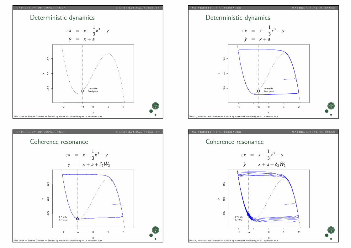
un i v er s i ty of copenhagen mathemat i ca l s c i ence s
Coherence resonance
εx = x − 1
3x3 − y
y = x + a + δ2W2
x
y
−0.
50.
00.
5
−2 −a 0 1 2
●a = 1.05δ2 = 0.02
Slide 23/34 — Susanne Ditlevsen — Statistik og matematisk modellering — 13. november 2014
un i ver s i ty of copenhagen mathemat i ca l s c i ence s
Coherence resonance
εx = x − 1
3x3 − y
y = x + a + δ2W2
x
y
−0.
50.
00.
5
−2 −a 0 1 2
●a = 1.35δ2 = 0.2
Slide 24/34 — Susanne Ditlevsen — Statistik og matematisk modellering — 13. november 2014

un i v er s i ty of copenhagen mathemat i ca l s c i ence s
Coherence resonance
εx = x − 1
3x3 − y
y = x + a + δ2W2
Condition for coherence resonance:
δ2 ≥ C
((a − 1)3
log(a − 1)−1
)1/2
for some constant C > 0 and δ2 small. In the limita→ 1+ and δ2 → 0 the deterministic cycle appears. Theperiod is the same as in the deterministic case.
Slide 25/34 — Susanne Ditlevsen — Statistik og matematisk modellering — 13. november 2014
un i ver s i ty of copenhagen mathemat i ca l s c i ence s
Self-induced stochastic resonance
εx = x − 1
3x3 − y +
√εδ1W1
y = x + a
Prepare for something completelydifferent!
The scaling√εδ1 guarantees that δ1 measures the
relative strength of the noise term compared to the driftirrespective of the value of ε.
Slide 26/34 — Susanne Ditlevsen — Statistik og matematisk modellering — 13. november 2014
un i v er s i ty of copenhagen mathemat i ca l s c i ence s
Self-induced stochastic resonance
εx = x − 1
3x3 − y +
√εδ1W1
y = x + a
For self-induced stochastic resonance it is NOT requiredto be close to the bifurcation point (it happens for1 < a <
√3).
The nearly deterministic limit cycle that appears isDIFFERENT from the cycle in the noise-free system.
Period and amplitude can be controlled by δ1 and ε!!!
Slide 27/34 — Susanne Ditlevsen — Statistik og matematisk modellering — 13. november 2014
un i ver s i ty of copenhagen mathemat i ca l s c i ence s
Self-induced stochastic resonance
εx = x − 1
3x3 − y +
√εδ1W1
y = x + a
We look for near-deterministic behavior. Thus δ1 → 0.Also the time scale separation ratio ε→ 0. Condition:
δ21 log ε−1 → C
for some constant C , which we can choose freely in aninterval depending on a. The choice gives amplitude andperiod of the deterministic oscillation.
Slide 28/34 — Susanne Ditlevsen — Statistik og matematisk modellering — 13. november 2014
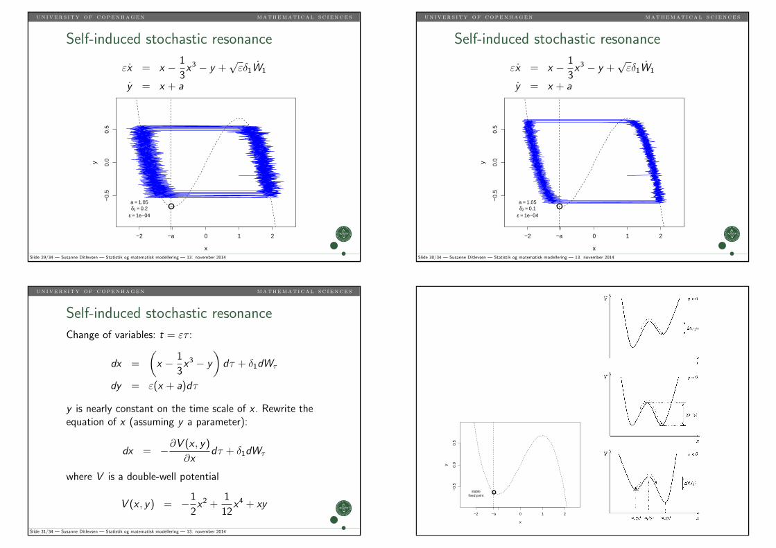
un i v er s i ty of copenhagen mathemat i ca l s c i ence s
Self-induced stochastic resonance
εx = x − 1
3x3 − y +
√εδ1W1
y = x + a
x
y
−0.
50.
00.
5
−2 −a 0 1 2
●a = 1.05δ2 = 0.2
ε = 1e−04
Slide 29/34 — Susanne Ditlevsen — Statistik og matematisk modellering — 13. november 2014
un i ver s i ty of copenhagen mathemat i ca l s c i ence s
Self-induced stochastic resonance
εx = x − 1
3x3 − y +
√εδ1W1
y = x + a
x
y
−0.
50.
00.
5
−2 −a 0 1 2
●a = 1.05δ2 = 0.1
ε = 1e−04
Slide 30/34 — Susanne Ditlevsen — Statistik og matematisk modellering — 13. november 2014
un i v er s i ty of copenhagen mathemat i ca l s c i ence s
Self-induced stochastic resonance
Change of variables: t = ετ :
dx =
(x − 1
3x3 − y
)dτ + δ1dWτ
dy = ε(x + a)dτ
y is nearly constant on the time scale of x . Rewrite theequation of x (assuming y a parameter):
dx = −∂V (x , y)
∂xdτ + δ1dWτ
where V is a double-well potential
V (x , y) = −1
2x2 +
1
12x4 + xy
Slide 31/34 — Susanne Ditlevsen — Statistik og matematisk modellering — 13. november 2014
x
y
−0.
50.
00.
5
−2 −a 0 1 2
●stablefixed point
first introduced by Freidlin for a model of a noise-drivenmechanical system in Ref. �22� �see also related early workin Refs. �32,33� in the context of stochastic resonance �34��.
In SISR, it is not required that a→1+. In fact, one canchoose any 1�a��3 and thus be far away from the bifur-cation threshold. Furthermore, the limit cycle is not the de-terministic one obtained in the limit as a→1−, and both itsphase portrait and its period can be controlled by a parameterdepending on �1 and �. Next we explain why this is so withan asymptotic argument.
As in CR, we require that �1→0 since this is the only wayto obtain a deterministic solution. We also let �→0. Thenthere exists an open interval I�a�, which depends on a, sothat if
�12ln �−1 → C2 �21�
for some constant C2� I�a� as �1→0 and �→0, a determin-istic limit cycle emerges. This limit cycle can be understoodas the result of keeping the system in a state of perpetualfrustration. The system tries to reach the fixed point �x� ,y��by sliding down SL, but each time it gets kicked by the noisetowards SR before reaching �x� ,y��. The system then slidesup SR, gets kicked toward SL before reaching the knee, andagain starts sliding down toward �x� ,y��. It can then repeatthis cycle.
To understand the jumping mechanism, we first make thechange of variables t=��, to get
dx = �x − 13x3 − y�d� + �1dW�, �22a�
dy = ��x + a�d� . �22b�
Equation �22a� is of the form
dx = −�V�x,y�
�xd� + �1dW�,
where V is a double-well potential
V�x,y� = − 12x2 + 1
12x4 + xy . �23�
Since y is nearly constant on this time scale from �22b�, yenters merely as a parameter in �23�. Viewed as a function ofx with y fixed, V�x ,y� is a double-well potential with twominima located at the value of x where SL and SR intersectthe horizontal line y=const, and a maximum at the intersec-tion with the unstable branch of the x nullcline �see Fig. 7�.To be more precise, let us define, for y� �− 2
3 , 23
�, the threeroots
x−�y� � x0�y� � x+�y�
of y=x− 13x3. The points x±�y� are always local minima of the
potential, and x0�y� is a local maximum. We define
�V+�y� = V„x0�y�,y… − V„x+�y�,y… ,
�V−�y� = V„x0�y�,y… − V„x−�y�,y… .
In each case, �V±�y� is the potential difference between thelocal maximum x0�y�, and a local minimum x±�y�, see Fig. 7.The value of �V+�y� can be easily computed parametrically
in terms of x1=x+�y�. After some straightforward algebra, wehave
�V+ = −3
4+
�3
8x1�4 − x1
2�3/2 −3
8x1
2�2 − x12� , �24�
and by symmetry �V−�y�=�V+�−y�. The resulting curves areplotted in Fig. 8.
Going back to �22a� and �22b�, fix y�0 and choose x nearSR. This puts x in the basin of attraction of x+�y� �right well�.Due to the noise, the process can jump into the left well byhopping over the barrier. Since the potential barrier it needsto cross is of size �V+�y�, from Wentzell-Freidlin theory �1�we know that the crossing time will asymptotically be aPoisson process with intensity
��y� = C exp„− 2�V+�y�/�12… , �25�
where C is some prefactor. By this we mean that for large T,the probability of seeing a jump over the barrier is
Prob�jump at y� = 1 − e−��y�T.
FIG. 7. Schematics of the potential V�x ,y� for different valuesof y.
DEVILLE, VANDEN-EIJNDEN, AND MURATOV PHYSICAL REVIEW E 72, 031105 �2005�
031105-6

un i v er s i ty of copenhagen mathemat i ca l s c i ence s
Self-induced stochastic resonance
The crossing time of the potential barrier ∆V+(y) isasymptotically a Poisson process with intensity
λ(y) ∝ exp{−2∆V+(y)/δ21}
y moves along the slow manifolds on the time scale ofε−1.
When the two time scales match at some y = y1, theprocess jumps. Before: infinite waiting time. After: timescale of jumps exponentially faster and it jumps. Happensalways very close to y1.
Slide 33/34 — Susanne Ditlevsen — Statistik og matematisk modellering — 13. november 2014
un i ver s i ty of copenhagen mathemat i ca l s c i ence s
SRP projekt, LMFK-bladet 4/2014
Slide 34/34 — Susanne Ditlevsen — Statistik og matematisk modellering — 13. november 2014