
Marching orders for QCD - ippp.dur.ac.uk · Marching orders for QCD – p.3. The challenge The...
46
Marching orders for QCD UK Annual theory meeting, December 19-21, 2005. Keith Ellis [email protected] Fermilab/CERN Slides available at http://theory.fnal.gov/people/ellis/Talks/ Marching orders for QCD – p.1
Transcript of Marching orders for QCD - ippp.dur.ac.uk · Marching orders for QCD – p.3. The challenge The...

Marching orders for QCD
UK Annual theory meeting, December 19-21,2005.
Keith Ellis
Fermilab/CERN
Slides available at http://theory.fnal.gov/people/ellis/Talks/
Marching orders for QCD – p.1
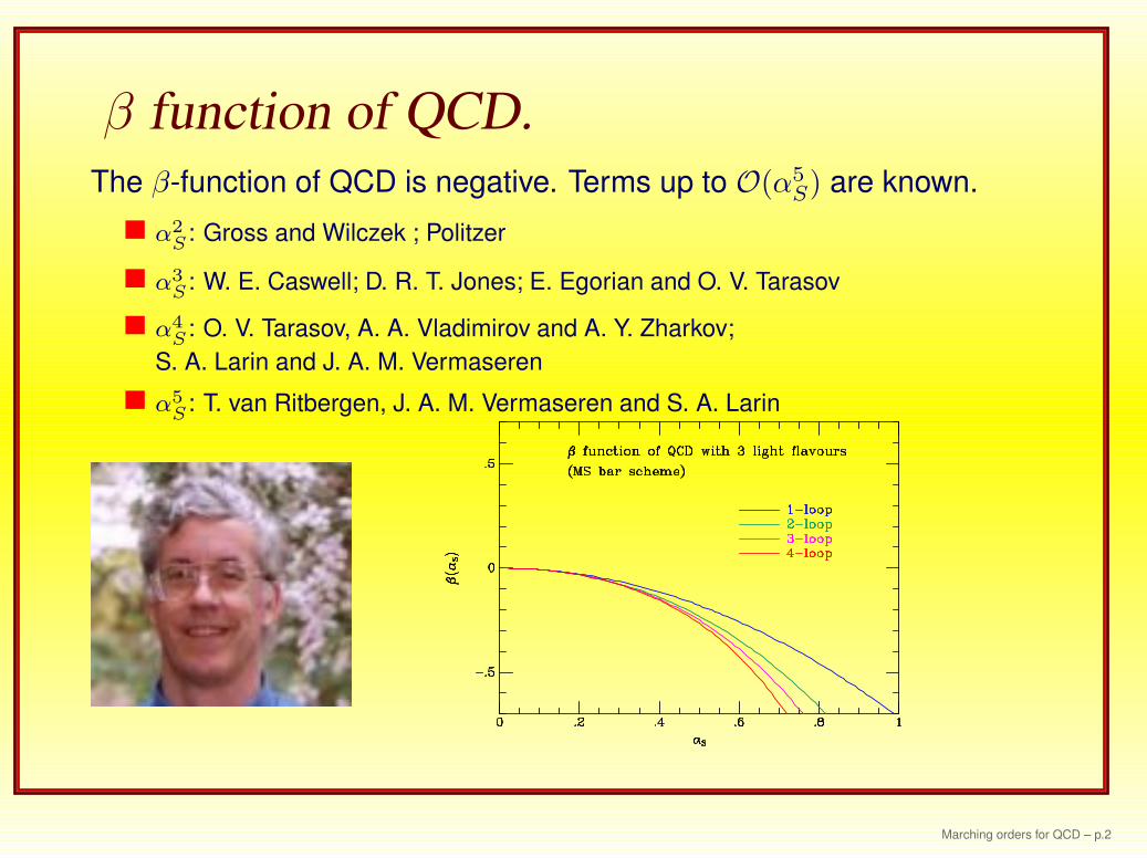
β function of QCD.
The β-function of QCD is negative. Terms up to O(α5S) are known.
α2
S: Gross and Wilczek ; Politzer
α3
S : W. E. Caswell; D. R. T. Jones; E. Egorian and O. V. Tarasov
α4
S: O. V. Tarasov, A. A. Vladimirov and A. Y. Zharkov;
S. A. Larin and J. A. M. Vermaseren
α5
S: T. van Ritbergen, J. A. M. Vermaseren and S. A. Larin
Marching orders for QCD – p.2

Current experimental results on αSBethke,hep-ph/0407021
jets & shapes 161 GeV
jets & shapes 172 GeV
0.08 0.10 0.12 0.14
(((( ))))s Z
-decays [LEP]
xF [ -DIS]F [e-, µ-DIS]
decays
(Z --> had.) [LEP]
e e [ ]+had
_e e [jets & shapes 35 GeV]+ _
(pp --> jets)
pp --> bb X
0
QQ + lattice QCD
DIS [GLS-SR]
2
3
pp, pp --> X
DIS [Bj-SR]
e e [jets & shapes 58 GeV]+ _
jets & shapes 133 GeV
e e [jets & shapes 22 GeV]+ _
e e [jets & shapes 44 GeV]+ _
e e [ ]+had
_
jets & shapes 183 GeV
DIS [pol. strct. fctn.]
jets & shapes 189 GeV
e e [scaling. viol.]+ _
jets & shapes 91.2 GeV
e e F+ _2
e e [jets & shapes 14 GeV]+ _
e e [4-jet rate]+ _
jets & shapes 195 GeVjets & shapes 201 GeVjets & shapes 206 GeV
DIS [ep –> jets]
αS(MZ) =
0.1182 ± 0.0027, MS, NNLO
QCD ( ) =s Z 0.1183 ± 0.00270.1
0.2
0.3
0.4
s(Q)
1 10 100Q [GeV]
LEPPETRA
TRISTAN
The decrease of αS is quite slow– as the inverse power of alogarithm.
αS is large at current scales.
Higher order corrections are im-portant.
Marching orders for QCD – p.3

The challenge
The challenge is to provide the most accurate information
possible to experimenters working at the Tevatron and the LHC.
Proton (anti)proton collisions give rise to a rich event structure.
Complexity of the events will increase as we pass from theTevatron to the LHC.
The goals
? To provide physics software tools which are both flexible andgive the most accurate representations of the underlyingtheories.
? To discover new efficient ways of calculating in perturbative
QCD.
Marching orders for QCD – p.4
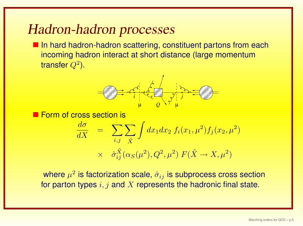
Hadron-hadron processesIn hard hadron-hadron scattering, constituent partons from each
incoming hadron interact at short distance (large momentum
transfer Q2).
� � � � �� � � � �� � � � �� � � � �� � � � �
� � � �� � � �� � � �� � � �
� � � � �� � � � �� � � � �� � � � �
� � � �� � � �� � � �� � � �� �� �� �� � � � � �
� � � �� � � �� � � �� � � �
� � �� � �� � �� � �� �� �
� �� �� �� �
� �� �� �� �
� �
� � � � � � � � � � � � � �� � � � � � � � � � � � �� � � � � �� � �� � �
����
���
���
����
���
���
j
Qµ µ
i
Form of cross section isdσ
dX=
∑
i,j
∑
X
∫
dx1dx2 fi(x1, µ2)fj(x2, µ
2)
× σXij (αS(µ2), Q2, µ2) F (X → X, µ2)
where µ2 is factorization scale, σij is subprocess cross section
for parton types i, j and X represents the hadronic final state.
Marching orders for QCD – p.5
Hadron-hadron processes II
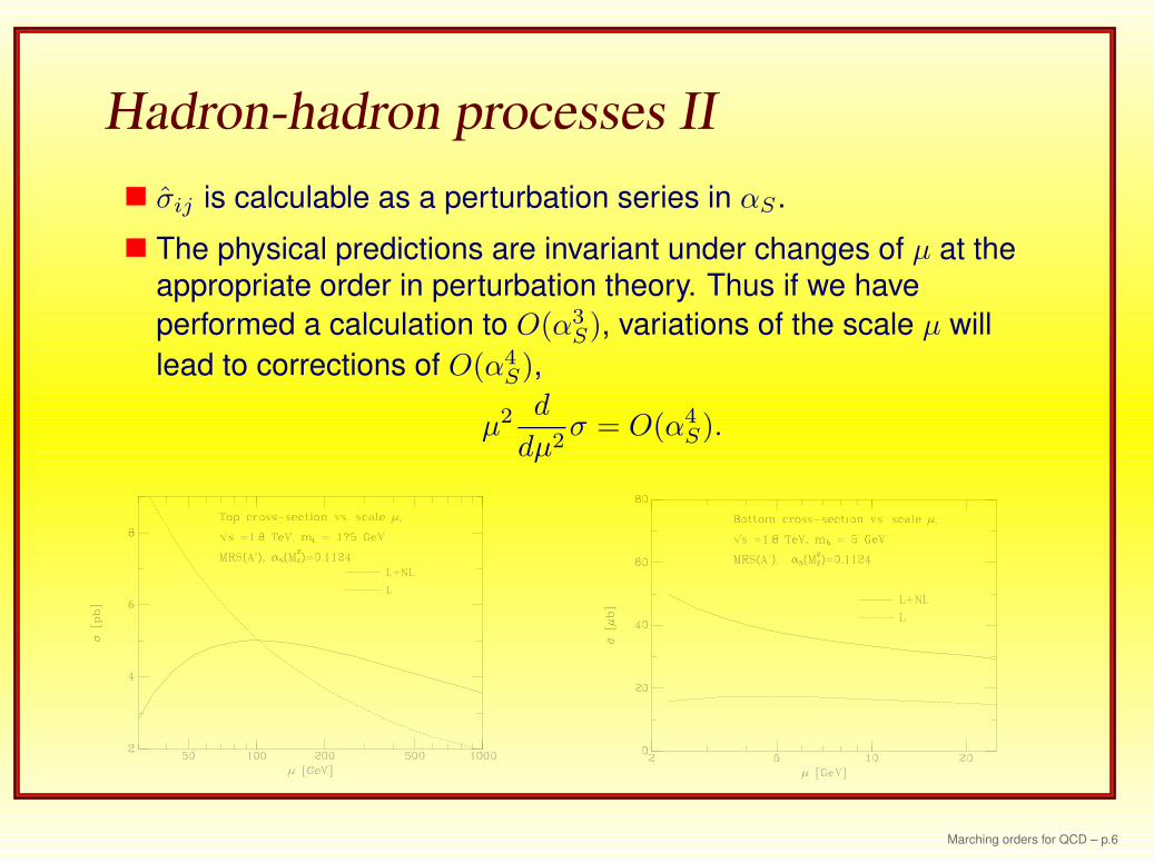
σij is calculable as a perturbation series in αS .
The physical predictions are invariant under changes of µ at theappropriate order in perturbation theory. Thus if we have
performed a calculation to O(α3S), variations of the scale µ will
lead to corrections of O(α4S),
µ2 d
dµ2σ = O(α4
S).
Marching orders for QCD – p.6
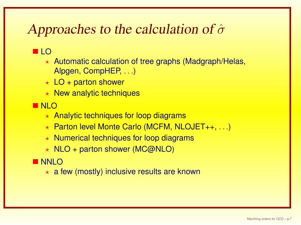
Approaches to the calculation of σ
LO
? Automatic calculation of tree graphs (Madgraph/Helas,
Alpgen, CompHEP, . . .)
? LO + parton shower
? New analytic techniques
NLO
? Analytic techniques for loop diagrams
? Parton level Monte Carlo (MCFM, NLOJET++, . . .)
? Numerical techniques for loop diagrams
? NLO + parton shower (MC@NLO)
NNLO
? a few (mostly) inclusive results are known
Marching orders for QCD – p.7
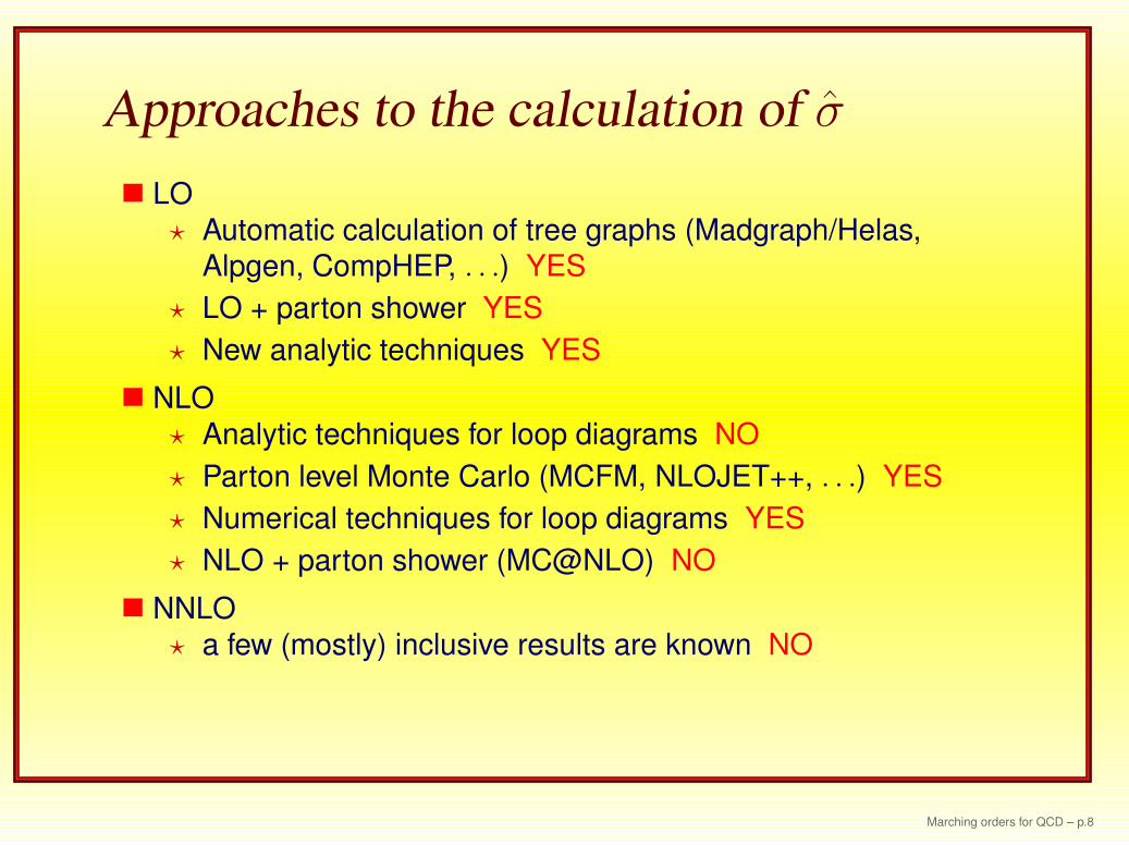
Approaches to the calculation of σ
LO
? Automatic calculation of tree graphs (Madgraph/Helas,
Alpgen, CompHEP, . . .) YES
? LO + parton shower YES
? New analytic techniques YES
NLO
? Analytic techniques for loop diagrams NO
? Parton level Monte Carlo (MCFM, NLOJET++, . . .) YES
? Numerical techniques for loop diagrams YES
? NLO + parton shower (MC@NLO) NO
NNLO
? a few (mostly) inclusive results are known NO
Marching orders for QCD – p.8

Multijet rates using tree graphs
Calculation of tree graphs using off-shell recurrence relations is asolved problem Berends, Giele.
Draggiotis et al
At 1033 cm−2s−1, lefthand scale gives eventsper second
g = 1
Similar calculations arepossible with other pro-grams Madgraph, Alp-gen, COMPHEP, . . .
Marching orders for QCD – p.9
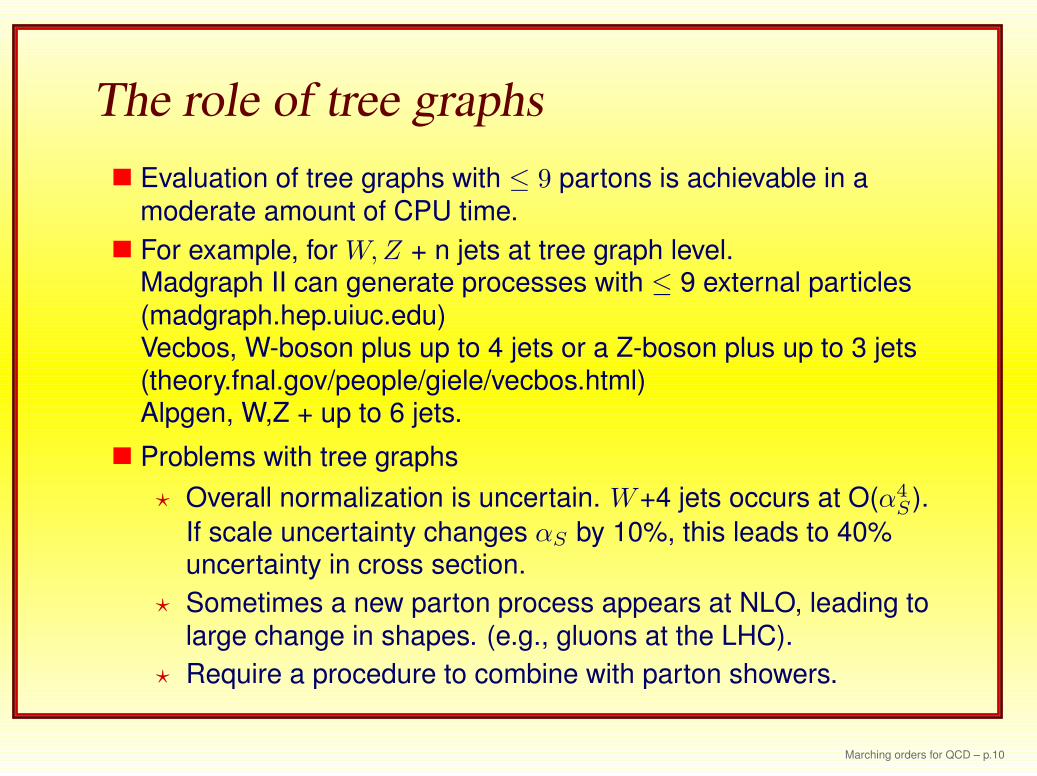
The role of tree graphs
Evaluation of tree graphs with ≤ 9 partons is achievable in a
moderate amount of CPU time.
For example, for W, Z + n jets at tree graph level.Madgraph II can generate processes with ≤ 9 external particles
(madgraph.hep.uiuc.edu)Vecbos, W-boson plus up to 4 jets or a Z-boson plus up to 3 jets(theory.fnal.gov/people/giele/vecbos.html)Alpgen, W,Z + up to 6 jets.
Problems with tree graphs
? Overall normalization is uncertain. W+4 jets occurs at O(α4S).
If scale uncertainty changes αS by 10%, this leads to 40%uncertainty in cross section.
? Sometimes a new parton process appears at NLO, leading to
large change in shapes. (e.g., gluons at the LHC).
? Require a procedure to combine with parton showers.
Marching orders for QCD – p.10

Combining Matrix elements and parton
showers
20 40 60 80 100 120 140 160 180
pT (highest jet) [GeV]
10-5
10-4
10-3
10-2
10-1
1/σ
dσ
/dp
T [
1/G
eV]
MCFM NLOSherpa
Wj + X @ Tevatron
PDF: cteq6l
Cuts: pT
lep> 20 GeV, |ηlep
|<1
pT
jet> 15 GeV, |ηjet
|<2
pT
miss> 20 GeV
∆Rjj> 0.7
Divide phase space into tworegions – region I for jetproduction modeled by theappropriate matrix element,region II for jet evolution modeledby the parton shower.
Procedure to cancel the leadingdependence on separation pa-rameter (CKKW)
pT spectrum of the hardest jet in inclusive W+1 jet, using Matrixelement improved showering scheme.
Agreement in shape between exact NLO calculation and MEimproved shower (SHERPA). F. Krauss et al, hep-ph/0409106
Marching orders for QCD – p.11
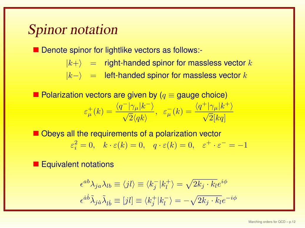
Spinor notation
Denote spinor for lightlike vectors as follows:-
|k+〉 = right-handed spinor for massless vector k
|k−〉 = left-handed spinor for massless vector k
Polarization vectors are given by (q ≡ gauge choice)
ε+µ (k) =
〈q−|γµ|k−〉√2〈qk〉
, ε−µ (k) =〈q+|γµ|k+〉√
2[kq]
Obeys all the requirements of a polarization vector
ε2i = 0, k · ε(k) = 0, q · ε(k) = 0, ε+ · ε− = −1
Equivalent notations
εabλjaλlb ≡ 〈jl〉 ≡ 〈k−j |k+
l 〉 =√
2kj · kleiφ
εabλjaλlb ≡ [jl] ≡ 〈k+j |k−
l 〉 = −√
2kj · kle−iφ
Marching orders for QCD – p.12

MHV amplitudes – 5 gluon amplitudeDecompose gluonic amplitude into color-ordered sub-amplitudes
A = Tr{ta1ta2ta3ta4ta5}m(1, 2, 3, 4, 5) + 23 permutations
Two of the color stripped amplitudes vanish
m(g+1 , g+
2 , g+3 , g+
4 , g+5 ) = 0
m(g−1 , g+2 , g+
3 , g+4 , g+
5 ) = 0
The maximal helicity violating 5 gluon amplitude
m(g−1 , g−2 , g+3 , g+
4 , g+5 ) =
〈12〉4〈12〉〈23〉〈34〉〈45〉〈51〉
〈ij〉, [ij] useful because QCD amplitudes have square root singularities.
Marching orders for QCD – p.13

MHV amplitudes
Parke and Taylor, Berends and Giele
The generalization to the case with two contiguous positivehelicity gluons and n − 2 negative gluons is
m(g−1 , g−2 , g+3 , . . . g+
n ) =〈12〉4
〈12〉〈23〉 . . . 〈n1〉
Remember 〈ij〉 are the spinor products ∼√
(2pi · pj)
Intuition from twistor space leads to two advances using spinors:
? Building more complicated amplitudes using effective MHVvertices.
? BCFW On-shell recursion relations.
Marching orders for QCD – p.14
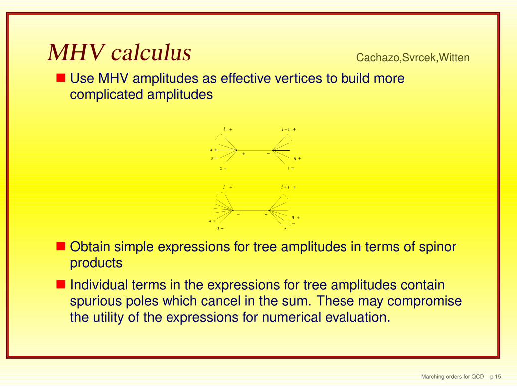
MHV calculus Cachazo,Svrcek,Witten
Use MHV amplitudes as effective vertices to build morecomplicated amplitudes
n +
1 −
+ −4 +
3 −
2 −
i ++i 1 +
− +
2 −
1 −
+n
3 −
4 +
i + i + 1 +
Obtain simple expressions for tree amplitudes in terms of spinorproducts
Individual terms in the expressions for tree amplitudes containspurious poles which cancel in the sum. These may compromisethe utility of the expressions for numerical evaluation.
Marching orders for QCD – p.15

On-shell recursion Britto et al, hep-th/0501052
Perform shift of the momenta conserving masslessness andoverall momentum conservation
pµ1 → pµ
1 = pµ1 − z
2〈1−|γµ|n−〉, pµ
n → pµn = pµ
n +z
2〈1−|γµ|n−〉
P 21,k = P 2
1,k − z〈1−|6Pi,k|n−〉, P1,k =k∑
j=1
pj
For each partition of momenta we obtain a pole zα
zα =P 2
1,k
〈1−|6Pi,k|n−〉
If the tree amplitudes, A(z), vanish for z → ∞ we can close the
contour on the integral 12πi
∮
cdzz A(z)
Marching orders for QCD – p.16

On-shell recursion
A(0) = −∑
poles α
Residuez=zα
A(z)
z
Atreen (1, 2, . . . , n) =
∑
h=±1
n−2∑
k=2
Atreek+1(1, 2, . . . , k,−P−h
1,k )i
P 21,k
× Atreen−k+1(P
h1,k, k + 1, . . . , n − 1, n).
Thus for the six gluon amplitude (220 diagrams) we have
A6(1+, 2+, 3+, 4−, 5−, 6−) =
i
〈2−|(6 + 1)|5−〉
×[ (〈6−|(1 + 2)|3−〉)3〈61〉〈12〉[34][45]s612
+(〈4−|(5 + 6)|1−〉)3〈23〉〈34〉[56][61]s561
]
notice unphysical singularities when the sum if 1+6 is a linear
combination of 2 and 5.
Marching orders for QCD – p.17

MHV outlook
Lead to beautiful results for gauge theory amplitudes; however the
evaluation of pure gluon tree graphs is a numerically solvedproblem, (Berends-Giele recursion).
Elegance of results relies on the introduction spurioussingularities; these can have a bearing on their numerical utility.
So far impact on real phenomenology limited; simple tree graph
results for Higgs+5 parton amplitudes Dixon et al, Badger et al
Extension to loops is the next frontier.
Marching orders for QCD – p.18
NLO
Marching orders for QCD – p.19

Why NLO?
The benefits of higher order calculations are:-
Less sensitivity to unphysical input scales (eg. renormalizationscale)
? First prediction of normalization of observables at NLO
? More accurate estimates of backgrounds for new physicssearches.
? Confidence that cross-sections are under control for precisionmeasurements
More physics
? Jet merging
? Initial state radiation
? More species of incoming partons enter at NLO
It represents the first step for other techniques matching withresummed calculations, eg. NLO parton showers
Marching orders for QCD – p.20
NLO calculation
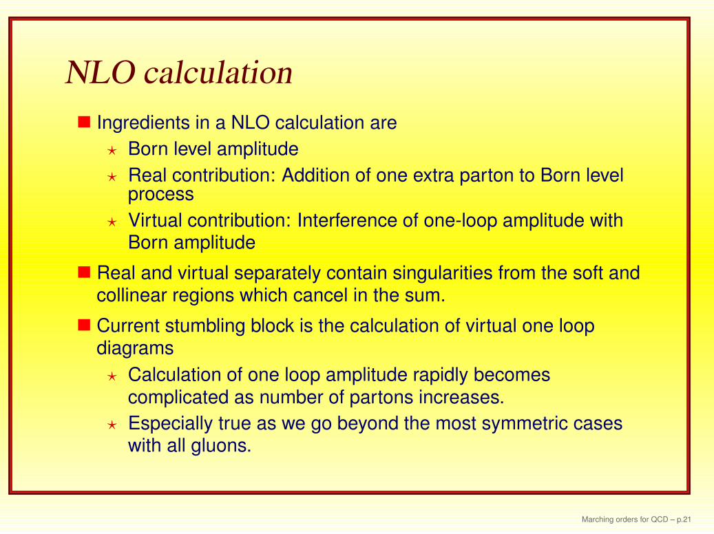
Ingredients in a NLO calculation are
? Born level amplitude
? Real contribution: Addition of one extra parton to Born levelprocess
? Virtual contribution: Interference of one-loop amplitude withBorn amplitude
Real and virtual separately contain singularities from the soft andcollinear regions which cancel in the sum.
Current stumbling block is the calculation of virtual one loopdiagrams
? Calculation of one loop amplitude rapidly becomescomplicated as number of partons increases.
? Especially true as we go beyond the most symmetric caseswith all gluons.
Marching orders for QCD – p.21
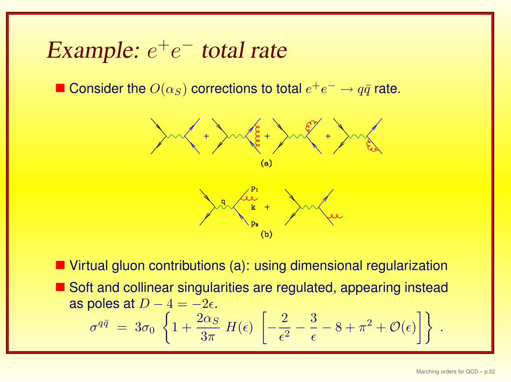
Example: e+e− total rate
Consider the O(αS) corrections to total e+e− → qq rate.
Virtual gluon contributions (a): using dimensional regularization
Soft and collinear singularities are regulated, appearing insteadas poles at D − 4 = −2ε.
σqq = 3σ0
{
1 +2αS
3πH(ε)
[
− 2
ε2− 3
ε− 8 + π2 + O(ε)
]}
.
Marching orders for QCD – p.22
Example: e+e− total rate
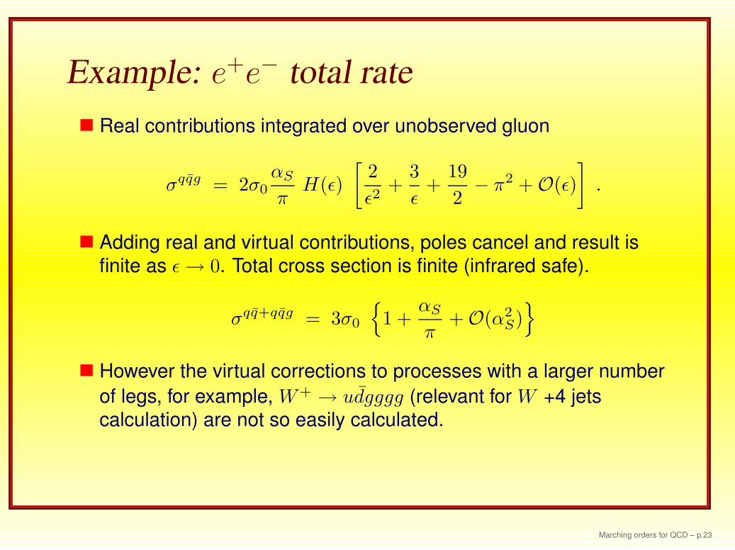
Real contributions integrated over unobserved gluon
σqqg = 2σ0
αS
πH(ε)
[
2
ε2+
3
ε+
19
2− π2 + O(ε)
]
.
Adding real and virtual contributions, poles cancel and result is
finite as ε → 0. Total cross section is finite (infrared safe).
σqq+qqg = 3σ0
{
1 +αS
π+ O(α2
S)}
However the virtual corrections to processes with a larger number
of legs, for example, W+ → udgggg (relevant for W +4 jets
calculation) are not so easily calculated.
Marching orders for QCD – p.23

Pure QCD amplitudes at one loop
Four parton processes
? qqq′q′ at one loop R.K. Ellis, Furman, Haber, Hinchliffe, 1980
? qqgg, gggg at one loop R.K. Ellis, Sexton, 1985
Five parton processes
? ggggg at one loop Bern et al, hep-ph/9302280
? qqggg at one loop Bern et al, hep-ph/9409393
? qqq′q′g at one loop Kunszt, hep-ph/9405386
Six parton processes
? Partial ggggg at one loop (completion expected in 2006)Bern et al, hep-ph/0505005,hep-ph/0505055,hep-ph/0507005,hep-ph/0412210
Britto et al hep-ph/0503132,Bedford et al, hep-th/0412108
? Advances in six parton amplitudes, using all the theoretical
tools, cut-constructibility, Susy (Yang-Mills) decomposition,BCFW recursion . . .
Marching orders for QCD – p.24

Decomposition of six gluon amplitude
Six gluon amplitude broken down in to simpler pieces
Agluon = AN=4 − 4AN=1 + Ascalar
where Agluon/scalar denotes an amplitude with only agluon/complex scalar running in the loop.
Because of their improved ultraviolet behaviour, thesupersymmetric pieces of the amplitude are cut-constructible. FullSUSY amplitude determined by the discontinuities, ie treediagrams
(a)
1
23
4
�
1 = p
p +
k4 p
− k
1
�
2 = p − k1 − k2
(b)
4 1
23
p
� 2 = p
+ k
4 1 =
p −
k1
p − k1 − k2
∫
dnp2πδ(p2)2πδ((p − k1 − k2)
2)
(p + k4)2(p − k1)2
→∫
dnp1
(p + k4)2p2(p − k1)2(p − k1 − k2)2
Marching orders for QCD – p.25

NLO Monte Carlo programs
Two programs for 3 jet production at Hadronic collidersKilgore, Giele, hep-ph/9610433, Nagy,hep-ph/0307268
The virtual corrections to the pure QCD processes are the easiestto calculate but the impact of processes leading to leptons, heavyquarks and missing energy is expected to be the larger.
Many low multiplicity processes involving vector bosons, topquarks, heavy quarks are included in the the parton level MonteCarlo program MCFM.
Marching orders for QCD – p.26

MCFM overviewJohn Campbell and R.K. Ellis
Parton level cross-sections predicted to NLO in αS
pp → W±/Z pp → W+ + W−
pp → W± + Z pp → Z + Zpp → W± + γ pp → W±/Z + Hpp → W± + g? (→ bb) pp → Zbbpp → W±/Z + 1 jet pp → W±/Z + 2 jets
pp(gg) → H pp(gg) → H + 1 jet
pp(V V ) → H + 2 jets pp → t + Xpp → t + W
⊕ less sensitivity to µR, µF , rates are better normalized, fullydifferential distributions.
low particle multiplicity (no showering), no hadronization, hard
to model detector effects
Marching orders for QCD – p.27

MCFM Information
Version 4.1 (January 05) available at:http://mcfm.fnal.gov
Improvements over previous releases:
? more processes (Z + b, single top, . . .)
? better user interface
? support for PDFLIB, Les Houches PDF accord(−→ PDF uncertainties)
? ntuples as well as histograms
? unweighted events
? Pythia/Les Houches generator interface (LO)
? separate variation of factorization and renormalization scales
? ‘Behind-the-scenes’ efficiency
Marching orders for QCD – p.28

W/Z+ jet cross-sections
The W/Z + 2 jet cross-section has been calculated at NLO and
should provide an interesting test of QCD (cf. many Run I studies
using the W/Z + 1 jet calculation in DYRAD)
For instance, the theoretical prediction for the number of eventscontaining 2 jets divided by the number containing only 1 is greatlyimproved.
Marching orders for QCD – p.29
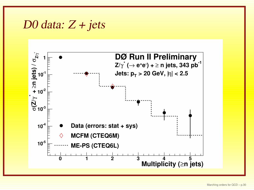
D0 data: Z + jets
n jets)≥Multiplicity (0 1 2 3 4 5
* γZ
/σ
n j
ets
) /
≥ +
*
γ(Z
/σ
-510
-410
-310
-210
-110
1 DØ Run II Preliminary-1
n jets, 343 pb≥) + -e+ e→ (*γZ/
| < 2.5η > 20 GeV, |TJets: p
Data (errors: stat + sys)
MCFM (CTEQ6M)
ME-PS (CTEQ6L)
Marching orders for QCD – p.30
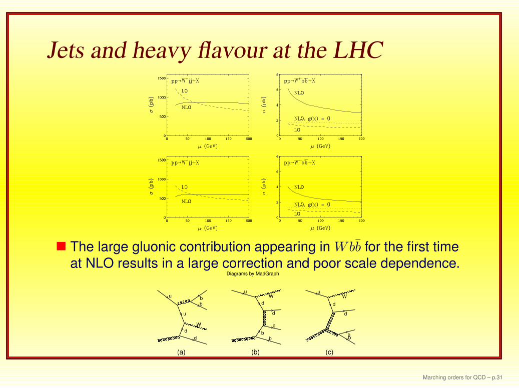
Jets and heavy flavour at the LHC
The large gluonic contribution appearing in Wbb for the first time
at NLO results in a large correction and poor scale dependence.
(a) (b) (c)
Diagrams by MadGraph
u
d
W
b b
d
u
u
d
W
b
b
d
b
u
d
W
b b
d
Marching orders for QCD – p.31

An experimenter’s wishlistRun II Monte Carlo Workshop
Single Boson Diboson Triboson Heavy Flavour
W+ ≤ 5j WW+ ≤ 5j WWW+ ≤ 3j tt+ ≤ 3jW + bb ≤ 3j W + bb+ ≤ 3j WWW + bb+ ≤ 3j tt + γ+ ≤ 2jW + cc ≤ 3j W + cc+ ≤ 3j WWW + γγ+ ≤ 3j tt + W+ ≤ 2jZ+ ≤ 5j ZZ+ ≤ 5j Zγγ+ ≤ 3j tt + Z+ ≤ 2jZ + bb+ ≤ 3j Z + bb+ ≤ 3j ZZZ+ ≤ 3j tt + H+ ≤ 2jZ + cc+ ≤ 3j ZZ + cc+ ≤ 3j WZZ+ ≤ 3j tb ≤ 2jγ+ ≤ 5j γγ+ ≤ 5j ZZZ+ ≤ 3j bb+ ≤ 3jγ + bb ≤ 3j γγ + bb ≤ 3jγ + cc ≤ 3j γγ + cc ≤ 3j
WZ+ ≤ 5jWZ + bb ≤ 3jWZ + cc ≤ 3jWγ+ ≤ 3jZγ+ ≤ 3j
Marching orders for QCD – p.32
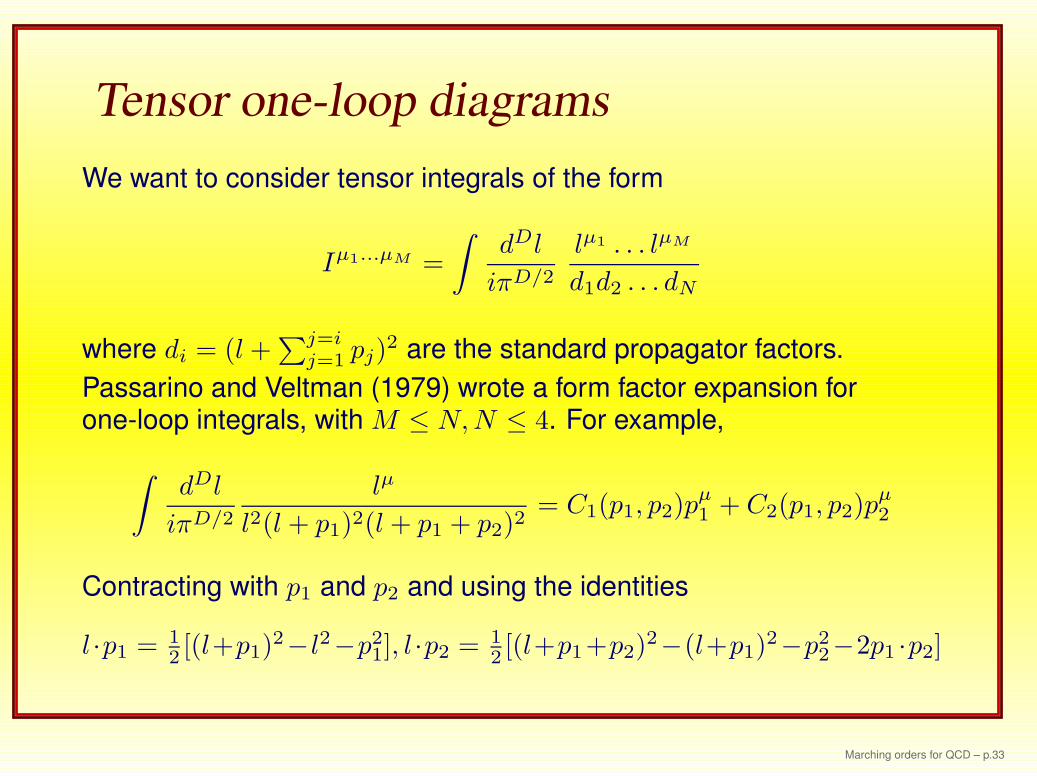
Tensor one-loop diagrams
We want to consider tensor integrals of the form
Iµ1...µM =
∫
dDl
iπD/2
lµ1 . . . lµM
d1d2 . . . dN
where di = (l +∑j=i
j=1 pj)2 are the standard propagator factors.
Passarino and Veltman (1979) wrote a form factor expansion forone-loop integrals, with M ≤ N, N ≤ 4. For example,
∫
dDl
iπD/2
lµ
l2(l + p1)2(l + p1 + p2)2= C1(p1, p2)p
µ1 + C2(p1, p2)p
µ2
Contracting with p1 and p2 and using the identities
l ·p1 = 12[(l+p1)
2−l2−p21], l ·p2 = 1
2[(l+p1+p2)
2−(l+p1)2−p2
2−2p1 ·p2]
Marching orders for QCD – p.33

Historical perspective II
We derive a linear equation expressing C1, C2 in terms of scalarintegrals
(
2p1 · p1 2p1 · p2
2p2 · p1 2p2 · p2
)(
C1
C2
)
=
(
R1
R2
)
where R1 = [B0(p1 + p2) − B0(p2) − p21 C0(p1, p2)]
and R2 = [B0(p1) − B0(p1 + p2) − (p22 + 2p1 · p2) C0(p1, p2)]
C0(p1, p2) =
∫
[dl]1
l2(l + p1)2(l + p1 + p2)2, B0(p1) =
∫
[dl]1
l2(l + p1)2
Solution involves the inverse of the Gram matrix, Gij ≡ 2pi · pj
G−1 =
(
+p2 · p2 −p1 · p2
−p1 · p2 +p1 · p1
)
/[2(p1 · p1 p2 · p2 − (p1 · p2)2)]
Marching orders for QCD – p.34

Historical perspective III
M. Veltman wrote a CDC program for numerical evaluation of the
formfactors in processes with only UV divergences, Utrecht(1979).
He dealt with exceptional regions, (e.g. regions where the Gram
determinant vanishes), by implementing parts of the program inquadruple precision.
Translation and improvement by Van Oldenborgh (1990) andfurther work on interface by T. Hahn and M. Perez-Victoria (1998).
However this is not sufficient for our needs.
We are interested in processes with more than 4 external legs.
We are often interested in loop processes with collinear and softsingularities due to the presence of massless particles. These are
most commonly (and elegantly) controlled by dimensionalregularization.
Marching orders for QCD – p.35

Bibliography, Tensor reduction
D. B. Melrose, Nuovo Cimento, 1965In a d dimensional space, a scalar diagram with n > d external
legs can be reduced to a sum of diagrams with d external legs.
Passarino and Veltman, Nucl. Phys. 1979
Binoth et al., hep-ph/0504267, hep-ph/9911342
Denner and Dittmaier, hep-ph/0509141
Giele and Glover, hep-ph/0402152, Giele and Glover andZanderighi hep-ph/0407016
Anastasiou and Daleo, hep-ph/0511176
Marching orders for QCD – p.36

Recursion relations I
Define generalized scalar integrals
di ≡ (l + qi)2
qi ≡i∑
j=1
pj
qN ≡N∑
j=1
pj = 0,
I(D; ν1, ν2, . . . , νN ) = I(D; {νk}Nk=1) ≡
∫
dD l
iπD/2
1
dν1
1 dν2
2 · · · dνN
N
,
Marching orders for QCD – p.37

Form-factor expansionDavydchev
For form factor expansion in terms of the q’s the coefficients aregeneralized scalar integrals in shifted dimensionalities
e.g., the rank-1 and rank-2 tensor integrals with N external legscan be decomposed as
Iµ1(D; q1, . . . , qN ) =N∑
i1=1
I(D + 2; {1 + δi1k}Nk=1) qµ1
i1
= I(D + 2; 2, 1, 1, . . . , 1) qµ1
1 + I(D + 2; 1, 2, 1, . . . , 1) qµ1
2
+ · · · + I(D + 2; 1, 1, 1, . . . , 2) qµ1
N .
Iµ1µ2(D; q1, . . . , qN ) = −1
2I(D + 2; 1, 1, 1, . . . , 1) gµ1µ2
+2 I(D + 4; 3, 1, 1, . . . , 1) qµ1
1 qµ2
1
+ I(D + 4; 2, 2, 1, . . . , 1) (qµ1
1 qµ2
2 + qµ2
1 qµ1
2 ) + · · ·
Marching orders for QCD – p.38

Basic identity Tkachev,Chetyrkin,Tarasov,Duplancic,Nizic
∫
dDl
iπD/2
∂
∂lµ
(
∑Ni=1 yi
)
lµ +(
∑Ni=1 yiq
µi
)
dν1
1 dν2
2 · · · dνN
N
= 0 .
valid for arbitrary yi. Differentiating we obtain the base identity
N∑
j=1
(
N∑
i=1
Sjiyi
)
νjI(D; {νk + δkj}Nk=1) = −
N∑
i=1
yiI(D − 2; {νk − δki}Nk=1)
−
D − 1 −N∑
j=1
νj
(
N∑
i=1
yi
)
I(D; {νk}Nk=1) ,
where S is a kinematic matrix which, for massless internal particles,takes the form
Sij ≡ (qi − qj)2.
Marching orders for QCD – p.39

Recursion relations II
Solving∑
i Sjiyi = δlj (assuming that the inverse of the matrix S
exists), we derive the basic recursion relation
(νl − 1)I(D; {νk}Nk=1)
= −N∑
i=1
S−1li I(D − 2; {νk − δik − δlk}N
k=1)
− bl (D − σ) I(D; {νk − δlk}Nk=1).
σ ≡N∑
i=1
νi; bi ≡N∑
j=1
S−1ij ; B ≡
N∑
i=1
bi =N∑
i,j=1
S−1ij .
The strategy is to reduce more complicated integrals to a set of simplerbasis integrals which are known analytically.Hence the method is seminumerical.
Marching orders for QCD – p.40

Recursion relations (cont)
Example: reduction of boxes, σ =∑
i νi
Using the basic identity (red lines) and other subsidiary identities
(blue and green lines) one can always arrive at the basis integral,
(four-dimensional box), denoted by a diamond, (or integrals withfewer external legs).
Marching orders for QCD – p.41

H+2 jet calculation
NLO corrections to W -fusion mechanism already calculated bymany authors.
All the elements are in place for a full NLO Higgs + 2 jets
calculation via gluon fusion mechanism
? Born level calculation Higgs + 4 partons
? Real calculation Higgs + 5 partons,Del Duca et al, Dixon et al, Badger et al
? Virtual calculation Ellis, Giele and Zanderighi, presented here
? Subtraction terms Campbell, Ellis and Zanderighi, in preparation
Marching orders for QCD – p.42

Proof of principleEllis, Giele, Zanderighi
Use the effective theory (mt → ∞) for Hgg coupling
Leff =1
4A(1 + ∆)HGa
µνGa µν .
Gaµν is the field strength of the gluon field and H is the Higgs-boson
field, A = g2
12π2v where g is the bare strong coupling and v is the
vacuum expectation value parameter, v2 = (GF
√2)−1 = (246 GeV)2.
∆ is a finite correction. Calculate virtual corrections to
A) H → qqq′q′, (30 diagrams),
B) H → qqqq, (60 diagrams),
C) H → qqgg, (191 diagrams),
D) H → gggg, (739 diagrams).
Marching orders for QCD – p.43

Method
Generate graphs and Form input using Qgraf
Write numerical result for each diagram in terms of
A(p1, . . . , pN ; ε1, . . . , εN ) =
N∑
M=0
Kµ1···µM(p1, . . . , pN ; ε1, . . . , εN )
Iµ1···µM (D; q1, . . . , qN ) ,
Reduce tensor integrals numerically to a set of basis integrals
(which are known analytically) by a recursive numericalprocedure.
Check the Ward identities numerically.
Generate complete matrix elements squared by summing over
squares of helicity amplitudes.
Marching orders for QCD – p.44

Comparison of numerical and analytic
results for H → four partons1
ε21
ε1
AB 0 0 12.9162958212387
AV,N -68.8869110466063 -114.642248172519 120.018444115458
AV,A -68.8869110466064 -114.642248172523 120.018444115429
BB 0 0 858.856417157052
BV,N -4580.56755817094 -436.142317955208 26470.9608978350
BV,A -4580.56755817099 -436.142317955660 26470.9608978346
CB 0 0 968.590160211857
CV,N -8394.44805516930 -19808.0396331354 -1287.90574949112
CV,A -8394.44805516942 -19808.0396331363 not known analytically
DB 0 0 3576991.27960852
DV,N -4.29238953553022 ·107 -1.04436372655580 ·10
8 -6.79830911471604·107
DV,A -4.29238953553022·107 -1.04436372655580 ·10
8 not known analytically
Marching orders for QCD – p.45

Current research directionsNLO is the first serious approximation in QCD. We shouldendeavour to calculate all interesting processes at this level.MCFM represents a start in this regard, but there is much left todo.
Stumbling block for higher leg processes: Virtual correctionsThere are two approaches to the evaluation of one-loop matrixelements
? Twistor ‘inspired’ Analytic Methods
? Semi-numerical or numerical methods
We can envisage a synergy between these two approaches.
Calculation of Matrix elements is not sufficient: Results must becast in a form where experimenters can use them.
Comparisons of all the Standard Model results amongst
themselves and with data is crucial both for the Tevatron and theLHC.
Marching orders for QCD – p.46