Received: 24 October 2018 Revised: 19 December 2018 Accepted: 16 January 2019

RE S EARCH ART I C L E

DOI: 10.1002/cem.3117

Local partial least squares based on global PLS scores

Guanghui Shen1,2 | Matthieu Lesnoff3,4 | Vincent Baeten2 | Pierre Dardenne2 |

Fabrice Davrieux5,6 | Hernan Ceballos7 | John Belalcazar7 | Dominique Dufour6,7,8,9 |

Zengling Yang1 | Lujia Han1 | Juan Antonio Fernández Pierna2

1College of Engineering, ChinaAgricultural University, Beijing, China2Food and Feed Quality Unit, Valorisationof Agricultural Products Department,Walloon Agricultural Research Center,Gembloux, Belgium3CIRAD, UMR SELMET, Montpellier,France4SELMET, Université de Montpellier,CIRAD, INRA, Montpellier Sup Agro,Montpellier, France5UMR Qualisud, CIRAD, Saint‐Denis,France6Qualisud, Université de Montpellier,CIRAD, Montpellier SupAgro, Universitéd'Avignon, Université de La Réunion,Montpellier, France7Cassava Program, International Centerfor Tropical Agriculture (CIAT), Cali,Colombia8UMR Qualisud, CIRAD, Cali, Colombia9UMR Qualisud, CIRAD, Montpellier,France

CorrespondenceJuan Antonio Fernández Pierna, Food andFeed Quality Unit, Valorisation ofAgricultural Products Department,Walloon Agricultural Research Center,Gembloux, Belgium.Email: foodfeedquality@cra.wallonie.be; j.fernandez@cra.wallonie.be

Funding informationChina Scholarship Council; HarvestPlus;CIRAD; CIAT

Journal of Chemometrics. 2019;e3117.https://doi.org/10.1002/cem.3117

Abstract

A local‐based method for near‐infrared spectroscopy predictions, the local

partial least squares regression on global PLS scores (LPLS‐S), is proposed in

this work and compared with the usual local PLS (LPLS) regression approach.

LPLS‐S is based on the idea of replacing the original spectra with a global PLS

score matrix before using the usual LPLS. This is done with the aim of increas-

ing the speed of the calculations, which can be an important parameter for

online applications in particular, especially when implemented on large

databases. In this study, the performance of the two local approaches was

compared in terms of efficiency and speed. It could be concluded that the

root‐mean‐square error of prediction of LPLS and LPLS‐S were 1.1962 and

1.1602, respectively, but the calculation speed for LPLS‐S was more than 20

times faster than for the LPLS algorithm.

KEYWORDS

local calibration, near‐infrared spectroscopy, partial least squares, running speed

1 | INTRODUCTION

Near‐infrared spectroscopy (NIRS), well known as a fast and nondestructive analytical method, is widely used incombination with partial least squares (PLS) for quality control and shows great potential for application in many fields,such as food (including fruits,1-3 dairy products,4 tea,5 meat,6 fish,7 and grain8,9), pharmaceuticals,10 biomass,11

© 2019 John Wiley & Sons, Ltd.wileyonlinelibrary.com/journal/cem 1 of 12

2 of 12 SHEN ET AL.

tobacco,12 and others. Generally speaking, conventional PLS (global PLS) calibration models can always provide satis-factory results when the relationship between the spectral and reference values is linear and the data are sufficient tocover all possible sources of variability. As Shenk et al suggested,13 the samples selected for model construction shouldinclude all possible sources of variation in terms of measurement factors (room temperature, operator, and instrumentsetup) but also in terms of sample population source (origin, process, varieties, storage conditions, and residualmoisture), which could increase the robustness of the calibration model. Based on these principles, extensive spectraldatabases compiling thousands of NIRS absorbance spectra have been created in recent years. In the case of the agricul-tural sector, the libraries relating to the monitoring of feed, grain, forage, and milk are the most extensive.

However, it is usually observed that the accuracy of the global calibration models (ie, a unique model fitted for allthe data set) decreases as complexity of the calibration set increases.13,14 To deal with this situation, multiple specificcalibrations for samples with a certain chemical composition or source can be developed to improve predictionaccuracy, but this can make the modeling process more complex when the categories within the database are very large.In view of these disadvantages, several alternatives based on local regression methods have been proposed. Localapproaches can be used to develop individual calibration models for each unknown sample to be predicted by selectingsimilar spectra from a large spectral library through distance or correlation.14,15

Of the existing local regression methods, comparison analyses using restructured near‐infrared and constituentdata,16 locally weighted regression (LWR),17 and the LOCAL algorithm patented by Shenk et al13 are the most widelyused when dealing with NIRS applications. Such methods try to deal with nonlinear or clustering problems occurringduring global model building. Comparison analyses using restructured near‐infrared and constituent, proposed byDavies et al, is a simple and rapid method, which predicts the value of an unknown sample by calculating a weightedaverage of the analytical reference values of the similar samples, selected based on r2 between the reduced and modifiedunknown spectrum and each spectrum in the database, compressed by a Fourier transformation.16 LWR was introducedby Cleveland and Devlin as a curve‐fitting method.17 It was then adapted for solving nonlinear problems in NIRS cal-ibration models. In particular, Naes et al18 and Næs and Isaksson,19 implemented LWR to local principal componentregression (PCR) models: for each sample to predict, a neighborhood of calibration samples is selected from a spectrallibrary based on Mahalanobis distances and a different weight is assigned to each calibration sample depending on itsdistance from the unknown sample. Later, Centner and Massart compared LWR using different regression methods(PCR and PLS), different distance measures (Euclidean and Mahalanobis distance), and different weighting schemes(uniform and cubic weighting) of calibration objects in local models to find an optimal combination.20 The LOCALalgorithm patented by Shenk and Westerhaus is another local regression method, which has been implemented incommercially available software.21 In the LOCAL algorithm, correlation coefficients between the spectrum of theunknown sample and those of the available database are calculated instead of Euclidean or Mahalanobis distances.The most similar samples used for the calibration models are selected with reference to a correlation threshold. Afterthe calibration data set has been defined, calibration models are performed by PLS regression.13

Besides the above‐mentioned methods, there are a few more recent local modeling approaches. Locally biasedregression, proposed by Fearn and Davies, uses two criteria to select the most similar spectra to an unknown spectrumfrom a database: the similarity of predicted values obtained by a global PLSR calibration and the spectral similarity,calculated by the score on the first orthogonal signal correction (OSC) factor in the same way as the PLSR prediction.The samples whose OSC scores lie in an interval around the OSC score defined by the predicted sample will be regardedas similar samples. Samples that pass both similarity tests are then selected as local samples for the new sample to bepredicted.22 Another method, the local central algorithm, uses principal component analysis (PCA) and theMahalanobis distance to select a training set and calculates the final prediction estimate using central tendency statisticssuch as the mean of the local neighbors for the unknown samples.23 Local calibration by percentile selection and localcalibration by customized radii selection are two novel algorithms for performing local regression based on PLSR thatselects samples by establishing a standardized radio around the projection of the unknown sample in the PLS scoresspace. The unknown sample is then predicted by weighting the regression coefficients and residuals obtained duringindividual (factor by factor) PLSR models.24

In NIRS applications, all the local approaches, including the above methods, face the problem of long calculationtime, in particular when the calibration data set contains a large number of samples. This is a strong constraint forthe model calibration abilities (especially when repeated Monte Carlo or bootstrap cross validation has to be imple-mented25) or for other applications such as online prediction platforms. The long calculation time is due first to thesearch of the neighbors (“KNN” selection) for each new sample and second to the fact that after each neighborhoodselection, a latent variables regression model (eg, PLSR or PCR) is fitted on the original spectral matrix of the neighbors

SHEN ET AL. 3 of 12

that is in general very wide. In this article, the approach that we propose for reducing the duration of the second step,and therefore of the overall process, is to fit the local latent variables regression model not on the original spectra of theneighbors but on already compressed data, containing a lower and limited number of columns. We implemented thisapproach in a local PLSR algorithm, in which the original spectra of each neighborhood were replaced by a matrix ofglobal PLS scores (the compressed data). The method was assessed on a real data set aiming to predict the nutritivequality of the cassava roots in Colombia. The study objectives were to estimate the effects of the preliminary datacompression (global PLS scores) in the local PLSR algorithm on the calculation time and the prediction efficiencies.

2 | MATERIAL AND METHODS

2.1 | Data set

Data used in this study for assessing the proposed local method come from a breeding program (Harvest Plus ChallengeProgram) on cassava plants monitored by the International Center for Tropical Agriculture in Colombia.26 One objec-tive of the program was to study and improve the nutritive quality of the cassava roots (see Davrieux et al26 for details).In particular, NIR spectra of fresh cassava root samples between 2009 and 2013 were recorded in duplicate from 400 to2498 nm at 2‐nm intervals using a FOSS 6500 monochromator with autocup sampling module (FOSS, Hillerod,Denmark), and the carotenoid contents were quantified through HPLC.

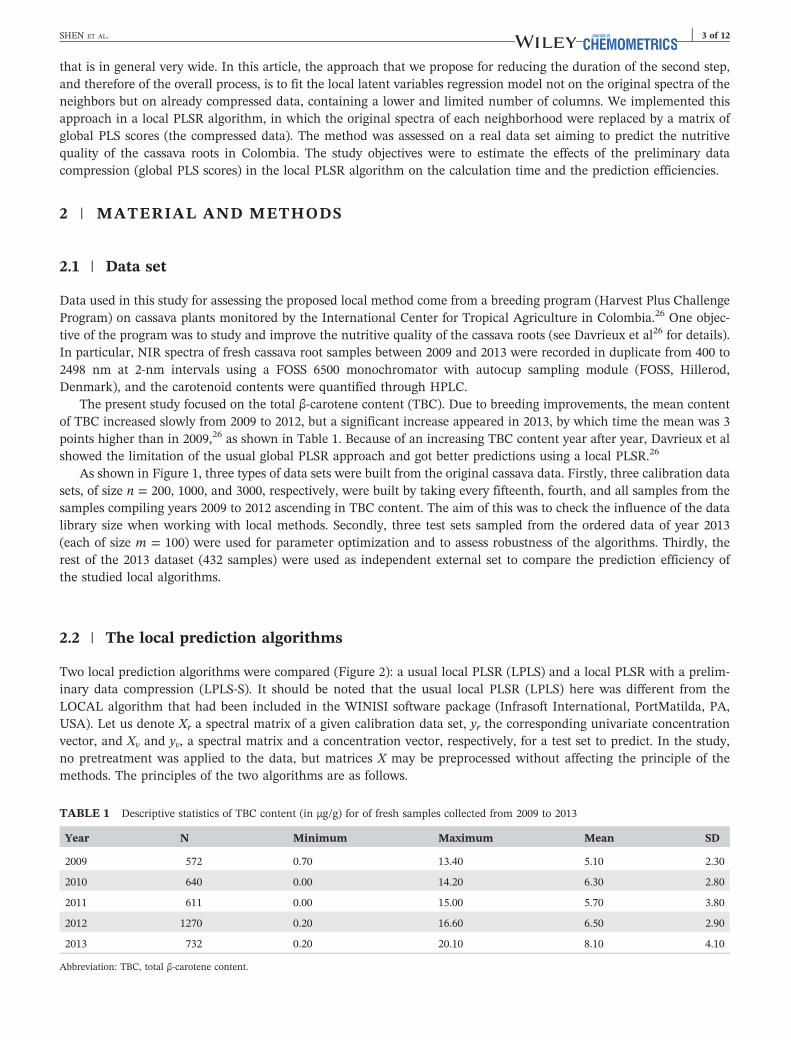
The present study focused on the total β‐carotene content (TBC). Due to breeding improvements, the mean contentof TBC increased slowly from 2009 to 2012, but a significant increase appeared in 2013, by which time the mean was 3points higher than in 2009,26 as shown in Table 1. Because of an increasing TBC content year after year, Davrieux et alshowed the limitation of the usual global PLSR approach and got better predictions using a local PLSR.26

As shown in Figure 1, three types of data sets were built from the original cassava data. Firstly, three calibration datasets, of size n = 200, 1000, and 3000, respectively, were built by taking every fifteenth, fourth, and all samples from thesamples compiling years 2009 to 2012 ascending in TBC content. The aim of this was to check the influence of the datalibrary size when working with local methods. Secondly, three test sets sampled from the ordered data of year 2013(each of size m = 100) were used for parameter optimization and to assess robustness of the algorithms. Thirdly, therest of the 2013 dataset (432 samples) were used as independent external set to compare the prediction efficiency ofthe studied local algorithms.

2.2 | The local prediction algorithms

Two local prediction algorithms were compared (Figure 2): a usual local PLSR (LPLS) and a local PLSR with a prelim-inary data compression (LPLS‐S). It should be noted that the usual local PLSR (LPLS) here was different from theLOCAL algorithm that had been included in the WINISI software package (Infrasoft International, PortMatilda, PA,USA). Let us denote Xr a spectral matrix of a given calibration data set, yr the corresponding univariate concentrationvector, and Xv and yv, a spectral matrix and a concentration vector, respectively, for a test set to predict. In the study,no pretreatment was applied to the data, but matrices X may be preprocessed without affecting the principle of themethods. The principles of the two algorithms are as follows.

TABLE 1 Descriptive statistics of TBC content (in μg/g) for of fresh samples collected from 2009 to 2013

Year N Minimum Maximum Mean SD

2009 572 0.70 13.40 5.10 2.30

2010 640 0.00 14.20 6.30 2.80

2011 611 0.00 15.00 5.70 3.80

2012 1270 0.20 16.60 6.50 2.90

2013 732 0.20 20.10 8.10 4.10

Abbreviation: TBC, total β‐carotene content.

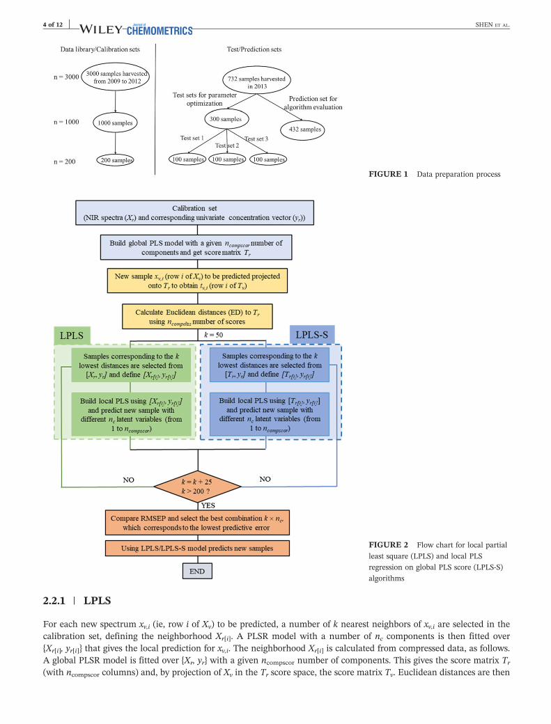
FIGURE 1 Data preparation process

FIGURE 2 Flow chart for local partial

least square (LPLS) and local PLS

regression on global PLS score (LPLS‐S)

algorithms

4 of 12 SHEN ET AL.

2.2.1 | LPLS

For each new spectrum xv,i (ie, row i of Xv) to be predicted, a number of k nearest neighbors of xv,i are selected in thecalibration set, defining the neighborhood Xr[i]. A PLSR model with a number of nc components is then fitted over{Xr[i], yr[i]} that gives the local prediction for xv,i. The neighborhood Xr[i] is calculated from compressed data, as follows.A global PLSR model is fitted over {Xr, yr} with a given ncompscor number of components. This gives the score matrix Tr

(with ncompscor columns) and, by projection of Xv in the Tr score space, the score matrix Tv. Euclidean distances are then

SHEN ET AL. 5 of 12

calculated between tv,i (ie, row i of Tv) and all the tr (ie, rows of Tr) using ncompdiss number of scores. The samplescorresponding to the k lowest distances are finally selected and define Xr[i].

The implementation of this process for all rows of Xv returns the y‐prediction vector for the single combinationk × nc. A predictive error estimate, such as root‐mean‐square error of prediction (RMSEP), is then calculated bycomparison with the observed data yv. The parameters k and nc can be optimized by defining a discrete grid over kand nc

20: the predictive error is calculated for each node of the grid, and the node with the lowest predictive errorcorresponds to the combination finally selected for the predictions. In this study, the grid was set to {k = 50, 75, …200} × {nc = 1, 2, …, 25}). The optimization was performed for each of the three test sets (of size m = 100) extracted fromthe 2013 data.

2.2.2 | LPLS‐S

In this algorithm, matrices Xr and Xv are first transformed to global PLS score matrices Tr and Tv, with a given ncompscor

number of components. The above LPLS algorithm is then simply run on Tr and Tv.

2.3 | Model comparison

The calculation time and the predictive efficiency were compared between LPLS and LPLS‐S for various values of theparameters ncompscor, ncompdiss, and n, the size of the data set (ie, number of samples) used for calibrating the algorithms,following a complete experiment design shown in Table 2. Three levels of global PLS scores (ncompscor: 3, 10 ,and 25)used for LPLS‐S, three different numbers of scores (ncompdiss: 3, 10, and 25) used for calculating distances, and threedifferent sizes for building the calibration data set (n = 200, 1000, and 3000) were combined. Predictions were donefor each test set (using models developed on the various calibration sets n = 200, 1000, and 3000) for the complete gridas shown in Table 2, and a final combination was selected corresponding to the lowest RMSEP in the grid.

TABLE 2 Experimental design for comparing both LPLS and LPLS‐S algorithms

Scenarios ncompscor ncompdiss k nc n m

1 3 3 50, 75 … 200 1, 2, 3 200 100

2 10 3 50, 75 … 200 1, 2, … 10 200 100

3 10 10 50, 75 … 200 1, 2, … 10 200 100

4 25 3 50, 75 … 200 1, 2, … 25 200 100

5 25 10 50, 75 … 200 1, 2, … 25 200 100

6 25 25 50, 75 … 200 1, 2, … 25 200 100

7 3 3 50, 75 … 200 1, 2, 3 1000 100

8 10 3 50, 75 … 200 1, 2, … 10 1000 100

9 10 10 50, 75 … 200 1, 2, … 10 1000 100

10 25 3 50, 75 … 200 1, 2, … 25 1000 100

11 25 10 50, 75 … 200 1, 2, … 25 1000 100

12 25 25 50, 75 … 200 1, 2, … 25 1000 100

13 3 3 50, 75 … 200 1, 2, 3 3000 100

14 10 3 50, 75 … 200 1, 2, … 10 3000 100

15 10 10 50, 75 … 200 1, 2, … 10 3000 100

16 25 3 50, 75 … 200 1, 2, … 25 3000 100

17 25 10 50, 75 … 200 1, 2, … 25 3000 100

18 25 25 50, 75 … 200 1, 2, … 25 3000 100

ncompscor (only LPLS‐S): number of global scores used for local partial least squares (PLS) regression on global PLS scores (LPLS‐S); ncompdiss: number of scoresused for calculating the distances; k: number of nearest neighbors; nc: number of latent variable for PLS models; n: number of samples in the calibration set; m:number of samples to be predicted.

6 of 12 SHEN ET AL.

All the data were processed using Matlab version 7.14 (The Mathworks, Inc., Natick, MA, USA) with thePLS_Toolbox version 8.0 (Eigenvector Research, Wenatchee, WA, USA). Computer configuration: Intel(R) Core (TM)I5‐7300HQ, CPU at 2.50 GHz, 8 GB random access memory, and 64‐bit operating system.

3 | RESULTS AND DISCUSSION

3.1 | PCA of samples

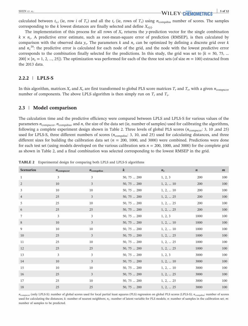
PCA was first applied to all the raw spectra of cassava samples harvested from 2009 to 2013. As shown in Figure 3, thePCA scores plot gave a cluster trend of different years' cassava samples. All the samples used in this study were clusteredinto four groups, which was due to the fact that year after year, cassava genotypes with higher dry matter and caroten-oid content were obtained by the breeding project, as reported by Davrieux et al.26

FIGURE 3 Principal component analysis scores plot for cassava samples collected from 2009 to 2013

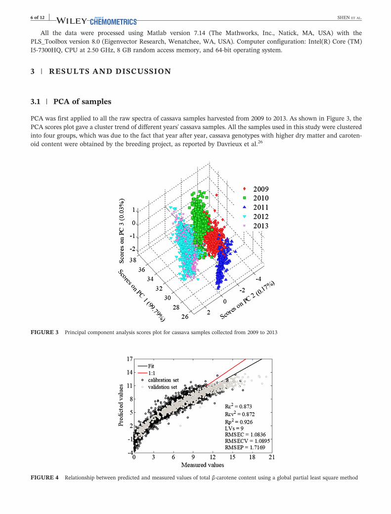
FIGURE 4 Relationship between predicted and measured values of total β‐carotene content using a global partial least square method

SHEN ET AL. 7 of 12

3.2 | Global PLS regression model

A global PLS regression model was built with samples harvested from 2009 to 2012 (total calibration set of 3000samples) and used to predict the independent prediction set of 432 samples (samples harvested in 2013). No pretreat-ment of data has been applied. The results are shown in Figure 4, where it can be seen that the root‐mean‐square errorof calibration and the root‐mean‐square error of cross validation were 1.084 and 1.089, respectively, meaning that thecalibration model was robust. However, a large RMSEP (1.7169) and a small relative percentage deviation (RPD = 2.39,RPD = SD/RMSEP) value appeared when new samples harvested in 2013 (gray in Figure 4) were predicted by thismodel. The RPD is usually used for testing the accuracy of NIRS calibration models, and RPD > 3 is consideredadequate for analytical purposes for agricultural products.27,28 RPD = 2.39 therefore indicated that a global PLSR model

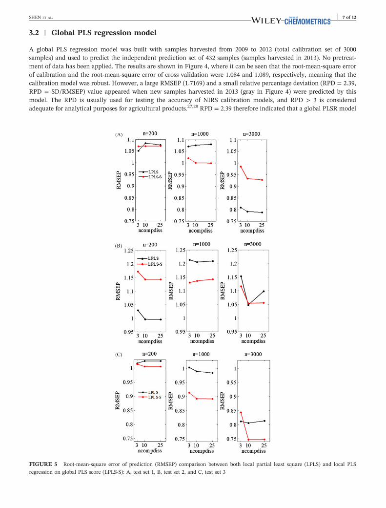
FIGURE 5 Root‐mean‐square error of prediction (RMSEP) comparison between both local partial least square (LPLS) and local PLS

regression on global PLS score (LPLS‐S): A, test set 1, B, test set 2, and C, test set 3

8 of 12 SHEN ET AL.

failed to properly predict new samples. Moreover, there was a clear nonlinear relationship between measured andpredicted values, especially for the higher TBC content, possibly because samples changed with the increasing contentof the constituent of interest year after year. In this case, the global PLSR model could not be used for the effectiveprediction of new harvested samples in 2013.

3.3 | LPLS and LPLS‐S algorithms

To address the poor prediction performance as well as the nonlinearity problem when using a global PLSR model, thetwo different locally based PLS regression algorithms (LPLS and LPLS‐S) were used and compared.

3.3.1 | Parameter optimization results for LPLS and LPLS‐S

The LPLS‐S algorithm was proposed for accelerating the prediction process based on global PLS scores. The runningtimes and efficiency of both LPLS and LPLS‐S algorithms were compared on the three test sets. The results aredisplayed in Tables S1 and S2 and Figure 5. All the results were acquired under the optimum combination of kand nc corresponding to the lowest RMSEP of the scenarios in Table 2 and for 25 global PLS scores when LPLS‐Swas used. As observed, the RMSEP values for LPLS show no distinct rule as the size of the calibration data (n) getslarger, but the running time increases significantly from 3.57 to 6.42 seconds. Unlike with the LPLS algorithm, theprediction precision for LPLS‐S increased with n, while the calculating time remained basically unchanged. On aver-age, when using 200, 1000, and 3000 calibration samples, the LPLS‐S algorithm was 13.04, 14.43, and 21.66 timesfaster than the LPLS method, respectively. This means that the more calibration samples there are in the calibrationdata set, the more obvious the advantage in running time for the LPLS‐S algorithm, with similar prediction perfor-mance. Besides, when the same calibration data set is used, the number of scores used for calculating distance(ncompdiss) has a very low effect on the running time of both LPLS and LPLS‐S algorithms but has a great impacton the prediction results.

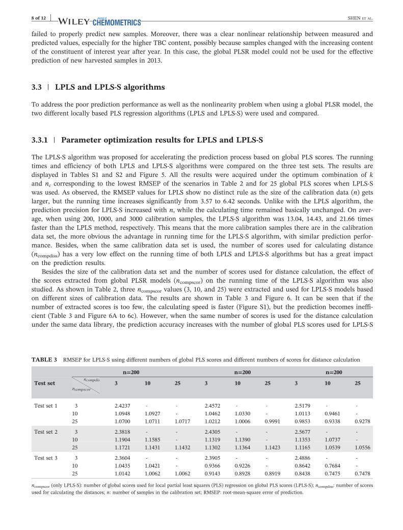
Besides the size of the calibration data set and the number of scores used for distance calculation, the effect ofthe scores extracted from global PLSR models (ncompscor) on the running time of the LPLS‐S algorithm was alsostudied. As shown in Table 2, three ncompscor values (3, 10, and 25) were extracted and used for LPLS‐S models basedon different sizes of calibration data. The results are shown in Table 3 and Figure 6. It can be seen that if thenumber of extracted scores is too few, the calculating speed is faster (Figure S1), but the prediction becomes ineffi-cient (Table 3 and Figure 6A to 6c). However, when the same number of scores is used for the distance calculationunder the same data library, the prediction accuracy increases with the number of global PLS scores used for LPLS‐S

TABLE 3 RMSEP for LPLS‐S using different numbers of global PLS scores and different numbers of scores for distance calculation

n=200 n=200 n=200

Test set 3 10 25 3 10 25 3 10 25

Test set 1 3 2.4237 ‐ ‐ 2.4572 ‐ ‐ 2.5179 ‐ ‐

10 1.0948 1.0927 ‐ 1.0462 1.0330 ‐ 1.0113 0.9461 ‐

25 1.0700 1.0711 1.0717 1.0212 1.0006 0.9991 0.9853 0.9338 0.9278

Test set 2 3 2.3818 ‐ ‐ 2.4305 ‐ ‐ 2.5677 ‐ ‐

10 1.1904 1.1585 ‐ 1.1319 1.1390 ‐ 1.1353 1.0737 ‐

25 1.1721 1.1431 1.1432 1.1302 1.1364 1.1423 1.1165 1.0539 1.0556

Test set 3 3 2.3604 ‐ ‐ 2.3905 ‐ ‐ 2.4886 ‐ ‐

10 1.0435 1.0421 ‐ 0.9366 0.9226 ‐ 0.8642 0.7684 ‐

25 1.0142 1.0062 1.0062 0.9143 0.8928 0.8919 0.8438 0.7475 0.7478

ncompscor (only LPLS‐S): number of global scores used for local partial least squares (PLS) regression on global PLS scores (LPLS‐S); ncompdiss: number of scoresused for calculating the distances; n: number of samples in the calibration set; RMSEP: root‐mean‐square error of prediction.

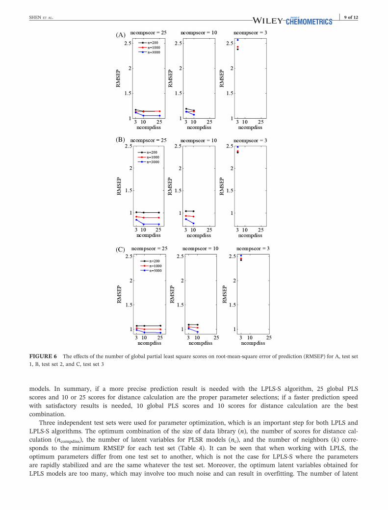
FIGURE 6 The effects of the number of global partial least square scores on root‐mean‐square error of prediction (RMSEP) for A, test set

1, B, test set 2, and C, test set 3

SHEN ET AL. 9 of 12

models. In summary, if a more precise prediction result is needed with the LPLS‐S algorithm, 25 global PLSscores and 10 or 25 scores for distance calculation are the proper parameter selections; if a faster prediction speedwith satisfactory results is needed, 10 global PLS scores and 10 scores for distance calculation are the bestcombination.

Three independent test sets were used for parameter optimization, which is an important step for both LPLS andLPLS‐S algorithms. The optimum combination of the size of data library (n), the number of scores for distance cal-culation (ncompdiss), the number of latent variables for PLSR models (nc), and the number of neighbors (k) corre-sponds to the minimum RMSEP for each test set (Table 4). It can be seen that when working with LPLS, theoptimum parameters differ from one test set to another, which is not the case for LPLS‐S where the parametersare rapidly stabilized and are the same whatever the test set. Moreover, the optimum latent variables obtained forLPLS models are too many, which may involve too much noise and can result in overfitting. The number of latent

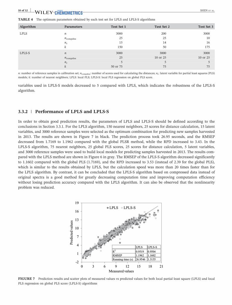
TABLE 4 The optimum parameters obtained by each test set for LPLS and LPLS‐S algorithms

Algorithm Parameters Test Set 1 Test Set 2 Test Set 3

LPLS n 3000 200 3000ncompdiss 25 25 10nc 15 14 16k 150 50 175

LPLS‐S n 3000 3000 3000ncompdiss 25 10 or 25 10 or 25nc 5 5 5k 50 or 75 75 75

n: number of reference samples in calibration set; ncompdiss: number of scores used for calculating the distances; nc: latent variable for partial least squares (PLS)models; k: number of nearest neighbors; LPLS: local PLS; LPLS‐S: local PLS regression on global PLS score.

10 of 12 SHEN ET AL.

variables used in LPLS‐S models decreased to 5 compared with LPLS, which indicates the robustness of the LPLS‐Salgorithm.

3.3.2 | Performance of LPLS and LPLS‐S

In order to obtain good prediction results, the parameters of LPLS and LPLS‐S should be defined according to theconclusions in Section 3.3.1. For the LPLS algorithm, 150 nearest neighbors, 25 scores for distance calculation, 15 latentvariables, and 3000 reference samples were selected as the optimum combination for predicting new samples harvestedin 2013. The results are shown in Figure 7 in black. The prediction process took 26.95 seconds, and the RMSEPdecreased from 1.7169 to 1.1962 compared with the global PLSR method, while the RPD increased to 3.43. In theLPLS‐S algorithm, 75 nearest neighbors, 25 global PLS scores, 25 scores for distance calculation, 5 latent variables,and 3000 reference samples were used to build local models for predicting samples harvested in 2013. The results com-pared with the LPLS method are shown in Figure 6 in gray. The RMSEP of the LPLS‐S algorithm decreased significantlyto 1.1602 compared with the global PLS (1.7169), and the RPD increased to 3.53 (instead of 2.39 for the global PLS),which is similar to the results obtained by LPLS, but the calculation speed was more than 20 times faster than forthe LPLS algorithm. By contrast, it can be concluded that the LPLS‐S algorithm based on compressed data instead oforiginal spectra is a good method for greatly decreasing computation time and improving computation efficiencywithout losing prediction accuracy compared with the LPLS algorithm. It can also be observed that the nonlinearityproblem was reduced.

FIGURE 7 Prediction results and scatter plots of measured values vs predicted values for both local partial least square (LPLS) and local

PLS regression on global PLS score (LPLS‐S) algorithms

SHEN ET AL. 11 of 12

4 | CONCLUSION

During the past few decades, a large number of local strategies have been proposed and showed good performance whendealing with nonlinearity problems encountered in global PLSR models. However, with the continuous accumulation ofdata, the database keeps increasing. This makes local strategies less useful, as the local algorithms need to establish ananalysis model for each sample, which requires a long calculation time. In this study, a new local strategy, LPLS‐S,based on compressed data (global PLS scores) instead of original spectra, was carefully investigated. The main conclu-sions derived from this research are that the prediction precision of the LPLS‐S algorithm increases when the databasebecomes larger and that between 10 and 25 global PLS scores are needed depending on the precision prediction/speedratio needed. Compared with the LPLS algorithm, LPLS‐S might lose prediction accuracy in some cases due to thepreliminary compression, but the calculation speed is greatly improved, and the more reference samples in the database,the more obvious the running time advantage for LPLS‐S. Also, this becomes an important output when workingwith online prediction systems. Moreover, in this study, the optimum parameters for the LPLS‐S algorithm are easierand more repeatable to be obtained whatever the test set than the LPLS algorithm. However, this should be validatedon other data sets. It should be mentioned that the local strategies permitted to correct the nonlinearity present inthe data.

In summary, all the results indicate that LPLS‐S has great potential to deal with huge data. Furthermore, the use ofthe global PLS scores to compress the original spectra was successfully applied to the local PLS method. The sameapproach could also be used for any other prediction methods, including support vector machines and neural networks,which have a reputation for being slow techniques.

ACKNOWLEDGEMENTS

This work was supported by the CIAT Cassava Project (Colombia) and CIRAD Qualisud Research Unit (France) andfunded mainly by HarvestPlus, c/o IFPRI (www.harvestplus.org), part of the Consultative Group on International Agri-culture Research (CGIAR), Program on Agriculture for Nutrition and Health (A4NH), project: “Enhancing the nutri-tional quality of cassava roots to improve the livelihoods of farmers in marginal agriculture land in Africa, Haiti, andNorth‐Colombia” and the CGIAR Research Program on Roots, Tubers and Bananas (RTB) (www.rtb.cgiar.org), project:“Driving livelihood improvements through demand‐oriented interventions for competitive production and processing ofRTBs” with support from CGIAR Trust Fund contributors (https://www.cgiar.org/funders/). The authors gratefullyacknowledge also financial support from the China Scholarship Council that allowed the author to work at the CRA‐W.

CONFLICT OF INTEREST

The authors declare no conflict of interest.

ORCID

Guanghui Shen https://orcid.org/0000-0002-9900-5586

REFERENCES

1. Nicolaï BM, Beullens K, Bobelyn E, et al. Nondestructive measurement of fruit and vegetable quality by means of NIR spectroscopy: areview. Postharvest Biol Technol. 2007;46(2):99‐118.

2. Magwaza LS, Opara UL, Nieuwoudt H, Cronje PJR, Saeys W, Nicolaï B. NIR spectroscopy applications for internal and external qualityanalysis of Citrus fruit—a review. Food Bioproc Tech. 2012;5(2):425‐444.

3. Pissard A, Fernández Pierna JA, Baeten V, et al. Non‐destructive measurement of vitamin C, total polyphenol and sugar content in applesusing near‐infrared spectroscopy. J Sci Food Agr. 2013;93(2):238‐244.

4. Laporte M, Paquin P. Near‐infrared analysis of fat, protein, and casein in cow's milk. J Agric Food Chem. 1999;47(7):2600‐2605.

5. Chen Q, Zhao J, Chaitep S, Guo Z. Simultaneous analysis of main catechins contents in green tea (Camellia sinensis (L.)) by Fouriertransform near infrared reflectance (FT‐NIR) spectroscopy. Food Chem. 2009;113(4):1272‐1277.

6. Kapper C, Klont RE, Verdonk JMAJ, Urlings HAP. Prediction of pork quality with near infrared spectroscopy (NIRS). Meat Sci.2012;91(3):294‐299.

12 of 12 SHEN ET AL.

7. Ru YJ, Glatz PC. Application of near infrared spectroscopy (NIR) for monitoring the quality of milk, cheese, meat and fish. Review. AsianAustral J Anim. 2000;7(13):1017‐1025.

8. Ferreira DS, Pallone JAL, Poppi RJ. Direct analysis of the main chemical constituents in Chenopodium quinoa grain using Fouriertransform near‐infrared spectroscopy. Food Control. 2015;48:91‐95.

9. Zhang C, Shen Y, Chen J, Xiao P, Bao J. Nondestructive prediction of total phenolics, flavonoid contents, and antioxidant capacity of ricegrain using near‐infrared spectroscopy. J Agric Food Chem. 2008;56(18):8268‐8272.

10. Roggo Y, Chalus P, Maurer L, Lema‐Martinez C, Edmond A, Jent N. A review of near infrared spectroscopy and chemometrics inpharmaceutical technologies. J Pharm Biomed Anal. 2007;44(3):683‐700.

11. Chadwick DT, McDonnell KP, Brennan LP, Fagan CC, Everard CD. Evaluation of infrared techniques for the assessment of biomass andbiofuel quality parameters and conversion technology processes: a review. Renew Sustain Energy Rev. 2014;30:672‐681.

12. Li Z, Li C, Gao Y, et al. Identification of oil, sugar and crude fiber during tobacco (Nicotiana tabacum L.) seed development based on nearinfrared spectroscopy. Biomass Bioenergy. 2018;111:39‐45.

13. Shenk JS, Westerhaus MO, Berzaghi P. Investigation of a LOCAL calibration procedure for near infrared instruments. J Near InfraredSpec. 1997;5(4):223‐232.

14. Berzaghi P, Shenk JS, Westerhaus MO. LOCAL prediction with near infrared multi‐product databases. J Near Infrared Spec. 2000;8(1):1‐9.

15. Godin B, Mayer F, Agneessens R, et al. Biochemical methane potential prediction of plant biomasses: comparing chemical compositionversus near infrared methods and linear versus non‐linear models. Bioresour Technol. 2015;175:382‐390.

16. Davies AM, Britcher HV, Franklin JG, Ring SM, Grant A, McClure WF. The application of fourier‐transformed near‐infrared spectra toquantitative analysis by comparison of similarity indices (CARNAC). Microchim Acta. 1988;1‐6(94):61‐64.

17. Cleveland WS, Devlin SJ. Locally weighted regression: an approach to regression analysis by local fitting. J Am Stat Assoc.1988;83(403):596‐610.

18. Naes T, Isaksson T, Kowalski B. Locally weighted regression and scatter correction for near‐infrared reflectance data. Anal Chem.1990;62(7):664‐673.

19. Næs T, Isaksson T. Locally weighted regression in diffuse near‐infrared transmittance spectroscopy. Appl Spectrosc. 1992;46(1):34‐43.

20. Centner V, Massart DL. Optimization in locally weighted regression. Anal Chem. 1998;70(19):4206‐4211.

21. Pérez Marín D, Garrido Varo A, Guerrero J. Non‐linear regression methods in NIRS quantitative analysis. Talanta. 2007;72(1):28‐42.

22. Fearn T, Davies AM. Locally‐biased regression. J Near Infrared Spec. 2003;11(6):467‐478.

23. Zamora Rojas E, Garrido Varo A, Van den Berg F, Guerrero Ginel JE, Pérez Marín D. Evaluation of a new local modelling approach forlarge and heterogeneous NIRS data sets. Chemometr Intell Lab. 2010;101(2):87‐94.

24. Allegrini F, Fernández Pierna JA, Fragoso WD, Olivieri AC, Baeten V, Dardenne P. Regression models based on new local strategies fornear infrared spectroscopic data. Anal Chim Acta. 2016;933:50‐58.

25. Filzmoser P, Liebmann B, Varmuza K. Repeated double cross validation. J Chemometrics: A Journal of the Chemometrics Society.2009;4(23):160‐171.

26. Davrieux F, Dufour D, Dardenne P, et al. LOCAL regression algorithm improves near infrared spectroscopy predictions when the targetconstituent evolves in breeding populations. J Near Infrared Spec. 2016;24(2):109‐117.

27. Williams PC. Implementation of near‐infrared technology. In: Williams P, Norris KH, eds. Near‐Infrared Technology in the Agriculturaland Food Industries. St. Paul, Minnesota, USA: American Association of Cereal Chemist; 2001:145‐169.

28. Cozzolino D, Morón A. Potential of near‐infrared reflectance spectroscopy and chemometrics to predict soil organic carbon fractions. SoilTillage Res. 2006;85(1‐2):78‐85.

SUPPORTING INFORMATION

Additional supporting information may be found online in the Supporting Information section at the end of the article.

How to cite this article: Shen G, Lesnoff M, Baeten V, et al. Local partial least squares based on global PLSscores. Journal of Chemometrics. 2019;e3117. https://doi.org/10.1002/cem.3117