Linear logic and deep learning - The Rising Seatherisingsea.org/notes/talk-lldl-transcript.pdf ·...

Linear logic and deep learningHuiyi Hu, Daniel Murfet

Good morning, and thankyou to the organisers for the opportunity to speak at this very interesting workshop. I should say upfront that I’m not a logician by training. If anything I’m an algebraic geometer, but I do a lot of category theory and its through that I encountered categorical semantics, and through that linear logic.

So I’ve been thinking about linear logic for a few years now, but when I started I was a postdoc at UCLA. A friend of mine Huiyi Hu was a PhD candidate in the applied math group working on machine learning, and the starting point for this joint project was her explaining some of the recent breakthroughs in that area.

She’s now at Google and her interests are quite applied, so we are trying to actually do something useful with this. But I’m only going to present the theoretical part of the project today, as the experimental component is still a work in progress.

So I’d like to begin by summarising some of the recent history in the field of artificial intelligence, or machine learning as its now called.

[1:20]

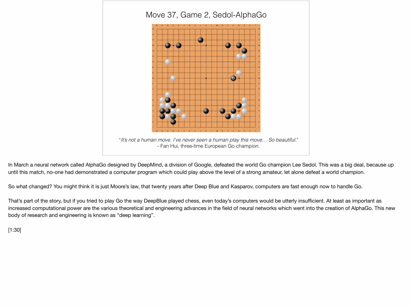
Move 37, Game 2, Sedol-AlphaGo

“It’s not a human move. I’ve never seen a human play this move… So beautiful.” - Fan Hui, three-time European Go champion.

In March a neural network called AlphaGo designed by DeepMind, a division of Google, defeated the world Go champion Lee Sedol. This was a big deal, because up until this match, no-one had demonstrated a computer program which could play above the level of a strong amateur, let alone defeat a world champion.

So what changed? You might think it is just Moore’s law, that twenty years after Deep Blue and Kasparov, computers are fast enough now to handle Go.

That’s part of the story, but if you tried to play Go the way DeepBlue played chess, even today’s computers would be utterly insufficient. At least as important as increased computational power are the various theoretical and engineering advances in the field of neural networks which went into the creation of AlphaGo. This new body of research and engineering is known as “deep learning”.

[1:30]

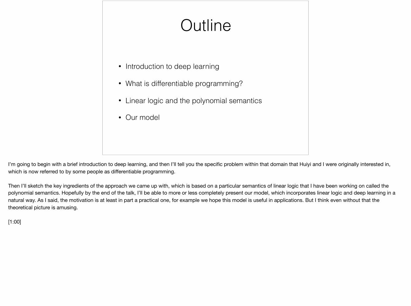
Outline

• Introduction to deep learning

• What is differentiable programming?

• Linear logic and the polynomial semantics

• Our model

I’m going to begin with a brief introduction to deep learning, and then I’ll tell you the specific problem within that domain that Huiyi and I were originally interested in, which is now referred to by some people as differentiable programming.

Then I’ll sketch the key ingredients of the approach we came up with, which is based on a particular semantics of linear logic that I have been working on called the polynomial semantics. Hopefully by the end of the talk, I’ll be able to more or less completely present our model, which incorporates linear logic and deep learning in a natural way. As I said, the motivation is at least in part a practical one, for example we hope this model is useful in applications. But I think even without that the theoretical picture is amusing.

[1:00]

A deep neural network (DNN) is a particular kind of function

Intro to deep learning

which depends in a “differentiable” way on a vector of weights.

Fw : Rm �! Rn

Example: Image classification, as in: cat or dog?

Fw

✓0.70.3

◆2 R2=

R685·685·3

2 pcat = 0.7

pdog

= 0.3

A deep neural network, or DNN or short, is a particular kind of function F_w from m-tuples of real numbers to n-tuples of real numbers for some m and n, which depends in a differentiable or smooth way on a vector of weights w. I’ll be more specific about what this class of functions looks like, and how they depend on the weights, in a few slides, but first I’d like to go through a couple of examples.

The first big application of deep neural nets was to image classification, that is, you’re given an image and the function needs to tell you what’s in it. An image can be represented as a vector by simply taking the RGB values of each pixel and reading them off into a list. So if this cat picture here was 685 pixels in width and height, with three colour channels, I’d need 685 squared times 3 real numbers to describe it completely.

The classification is also a vector, but of probabilities. If there are only two possible classes “dog” and “cat”, then the function outputs a column vector with the probability that the image lies in each class.

[1:30]


Fw : Rm �! Rn

Example: Playing the game of Go

2 8 J A N U A R Y 2 0 1 6 | V O L 5 2 9 | N A T U R E | 4 8 7

ARTICLE RESEARCH

better in AlphaGo than a value function ( )≈ ( )θ σv s v sp derived from the SL policy network.

Evaluating policy and value networks requires several orders of magnitude more computation than traditional search heuristics. To efficiently combine MCTS with deep neural networks, AlphaGo uses an asynchronous multi-threaded search that executes simulations on CPUs, and computes policy and value networks in parallel on GPUs. The final version of AlphaGo used 40 search threads, 48 CPUs, and 8 GPUs. We also implemented a distributed version of AlphaGo that

exploited multiple machines, 40 search threads, 1,202 CPUs and 176 GPUs. The Methods section provides full details of asynchronous and distributed MCTS.

Evaluating the playing strength of AlphaGoTo evaluate AlphaGo, we ran an internal tournament among variants of AlphaGo and several other Go programs, including the strongest commercial programs Crazy Stone13 and Zen, and the strongest open source programs Pachi14 and Fuego15. All of these programs are based

Figure 4 | Tournament evaluation of AlphaGo. a, Results of a tournament between different Go programs (see Extended Data Tables 6–11). Each program used approximately 5 s computation time per move. To provide a greater challenge to AlphaGo, some programs (pale upper bars) were given four handicap stones (that is, free moves at the start of every game) against all opponents. Programs were evaluated on an Elo scale37: a 230 point gap corresponds to a 79% probability of winning, which roughly corresponds to one amateur dan rank advantage on KGS38; an approximate correspondence to human ranks is also shown,

horizontal lines show KGS ranks achieved online by that program. Games against the human European champion Fan Hui were also included; these games used longer time controls. 95% confidence intervals are shown. b, Performance of AlphaGo, on a single machine, for different combinations of components. The version solely using the policy network does not perform any search. c, Scalability study of MCTS in AlphaGo with search threads and GPUs, using asynchronous search (light blue) or distributed search (dark blue), for 2 s per move.

3,500

3,000

2,500

2,000

1,500

1,000

500

0

c

1 2 4 8 16 32

1 2 4 8

12

64

24

112

40

176

64

280

40

Single machine Distributed

a

Rollouts

Value network

Policy network

3,500

3,000

2,500

2,000

1,500

1,000

500

0

b

40

8

Threads

GPUs

3,500

3,000

2,500

2,000

1,500

1,000

500

0

Elo

Rat

ing

GnuG

o

Fuego

Pachi

=HQ

Crazy S

tone

Fan Hui

AlphaG

o

AlphaG

odistributed

Professional dan (p)

Am

ateurdan (d)

Beginnerkyu (k)

9p7p5p3p1p

9d

7d

5d

3d

1d1k

3k

5k

7k

Figure 5 | How AlphaGo (black, to play) selected its move in an informal game against Fan Hui. For each of the following statistics, the location of the maximum value is indicated by an orange circle. a, Evaluation of all successors s′ of the root position s, using the value network vθ(s′); estimated winning percentages are shown for the top evaluations. b, Action values Q(s, a) for each edge (s, a) in the tree from root position s; averaged over value network evaluations only (λ = 0). c, Action values Q(s, a), averaged over rollout evaluations only (λ = 1).

d, Move probabilities directly from the SL policy network, ( | )σp a s ; reported as a percentage (if above 0.1%). e, Percentage frequency with which actions were selected from the root during simulations. f, The principal variation (path with maximum visit count) from AlphaGo’s search tree. The moves are presented in a numbered sequence. AlphaGo selected the move indicated by the red circle; Fan Hui responded with the move indicated by the white square; in his post-game commentary he preferred the move (labelled 1) predicted by AlphaGo.

Principal variation

Value networka

fPolicy network Percentage of simulations

b c Tree evaluation from rolloutsTree evaluation from value net

d e g

© 2016 Macmillan Publishers Limited. All rights reserved

Fw(current board) = 2 R19·19

2

R19⇥19



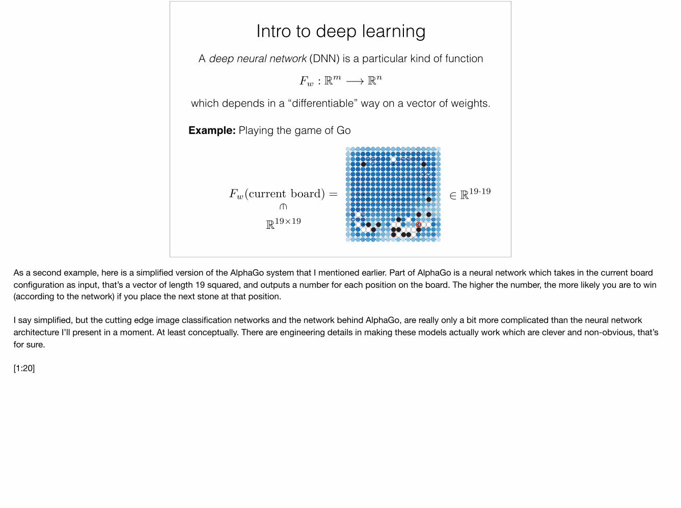
As a second example, here is a simplified version of the AlphaGo system that I mentioned earlier. Part of AlphaGo is a neural network which takes in the current board configuration as input, that’s a vector of length 19 squared, and outputs a number for each position on the board. The higher the number, the more likely you are to win (according to the network) if you place the next stone at that position.

I say simplified, but the cutting edge image classification networks and the network behind AlphaGo, are really only a bit more complicated than the neural network architecture I’ll present in a moment. At least conceptually. There are engineering details in making these models actually work which are clever and non-obvious, that’s for sure.

[1:20]

Ew =X

i

(Fw(xi)� yi)2

A randomly initialised neural network is trained on sample data

{(xi, yi)}i2I , xi 2 Rm, yi 2 Rn

by varying the weight vector in order to minimise the error


Fw : Rm �! Rn



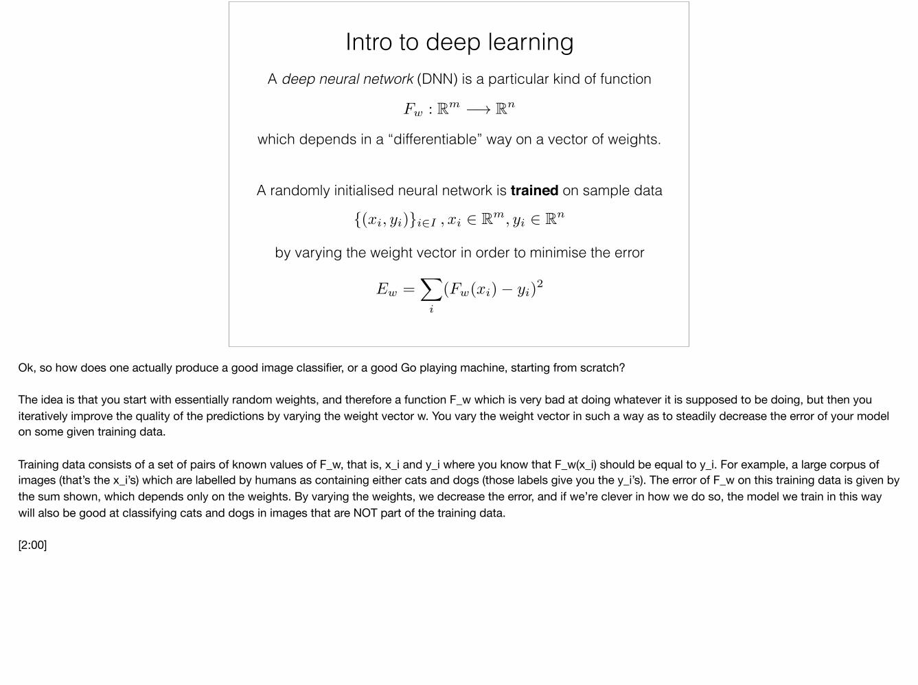
Ok, so how does one actually produce a good image classifier, or a good Go playing machine, starting from scratch?

The idea is that you start with essentially random weights, and therefore a function F_w which is very bad at doing whatever it is supposed to be doing, but then you iteratively improve the quality of the predictions by varying the weight vector w. You vary the weight vector in such a way as to steadily decrease the error of your model on some given training data.

Training data consists of a set of pairs of known values of F_w, that is, x_i and y_i where you know that F_w(x_i) should be equal to y_i. For example, a large corpus of images (that’s the x_i’s) which are labelled by humans as containing either cats and dogs (those labels give you the y_i’s). The error of F_w on this training data is given by the sum shown, which depends only on the weights. By varying the weights, we decrease the error, and if we’re clever in how we do so, the model we train in this way will also be good at classifying cats and dogs in images that are NOT part of the training data.

[2:00]

w1w2

optimal network

initial network

training process (gradient descent)

Ew

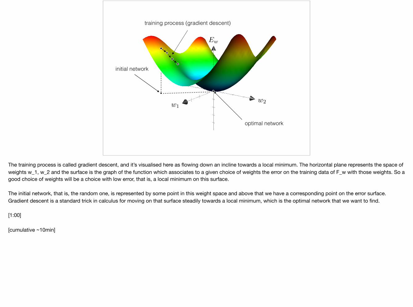
The training process is called gradient descent, and it’s visualised here as flowing down an incline towards a local minimum. The horizontal plane represents the space of weights w_1, w_2 and the surface is the graph of the function which associates to a given choice of weights the error on the training data of F_w with those weights. So a good choice of weights will be a choice with low error, that is, a local minimum on this surface.

The initial network, that is, the random one, is represented by some point in this weight space and above that we have a corresponding point on the error surface. Gradient descent is a standard trick in calculus for moving on that surface steadily towards a local minimum, which is the optimal network that we want to find.

[1:00]

[cumulative ~10min]

A DNN is made up of many layers of “neurons” connecting the input (on the left) to the output (on the right) as in the following diagram:

�(x) = 12 (x+ |x|)

x1 y1

wij

yixj

yi = �

⇣X

j

wijxj

⌘

w1j

w11


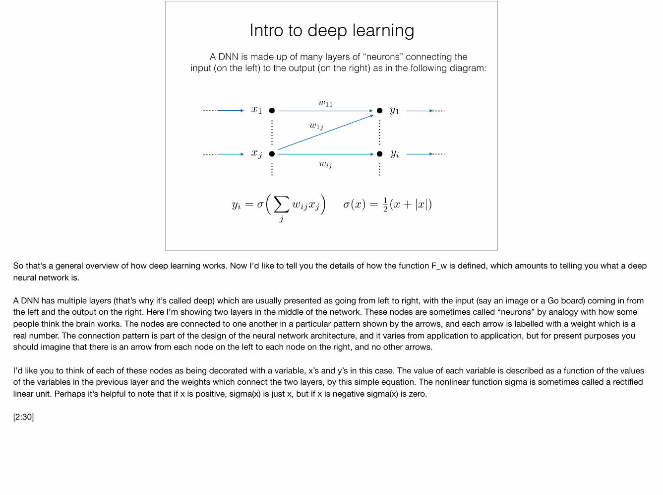
So that’s a general overview of how deep learning works. Now I’d like to tell you the details of how the function F_w is defined, which amounts to telling you what a deep neural network is.

A DNN has multiple layers (that’s why it’s called deep) which are usually presented as going from left to right, with the input (say an image or a Go board) coming in from the left and the output on the right. Here I’m showing two layers in the middle of the network. These nodes are sometimes called “neurons” by analogy with how some people think the brain works. The nodes are connected to one another in a particular pattern shown by the arrows, and each arrow is labelled with a weight which is a real number. The connection pattern is part of the design of the neural network architecture, and it varies from application to application, but for present purposes you should imagine that there is an arrow from each node on the left to each node on the right, and no other arrows.

I’d like you to think of each of these nodes as being decorated with a variable, x’s and y’s in this case. The value of each variable is described as a function of the values of the variables in the previous layer and the weights which connect the two layers, by this simple equation. The nonlinear function sigma is sometimes called a rectified linear unit. Perhaps it’s helpful to note that if x is positive, sigma(x) is just x, but if x is negative sigma(x) is zero.

[2:30]


�(x) = 12 (x+ |x|)

x1 y1

yixj

yi = �

⇣X

j

w

(k)ij xj

⌘

w(k)ij

w(k)1j

(k) (k + 1)w(k)11


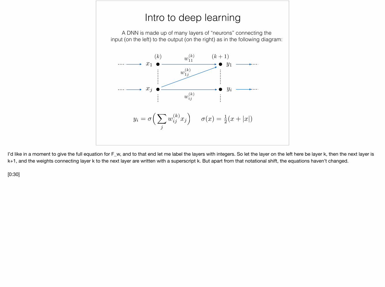
I’d like in a moment to give the full equation for F_w, and to that end let me label the layers with integers. So let the layer on the left here be layer k, then the next layer is k+1, and the weights connecting layer k to the next layer are written with a superscript k. But apart from that notational shift, the equations haven’t changed.

[0:30]


�(x) = 12 (x+ |x|)

x1 y1

yixj

w(k)ij

w(k)1j

~y = �

⇣W

(k)~x

⌘

(k) (k + 1)w(k)11


~x = (x1, x2, . . . , xj , . . .)T W (k) = (w(k)

ij )i,j

yi = �

⇣X

j

w

(k)ij xj

⌘

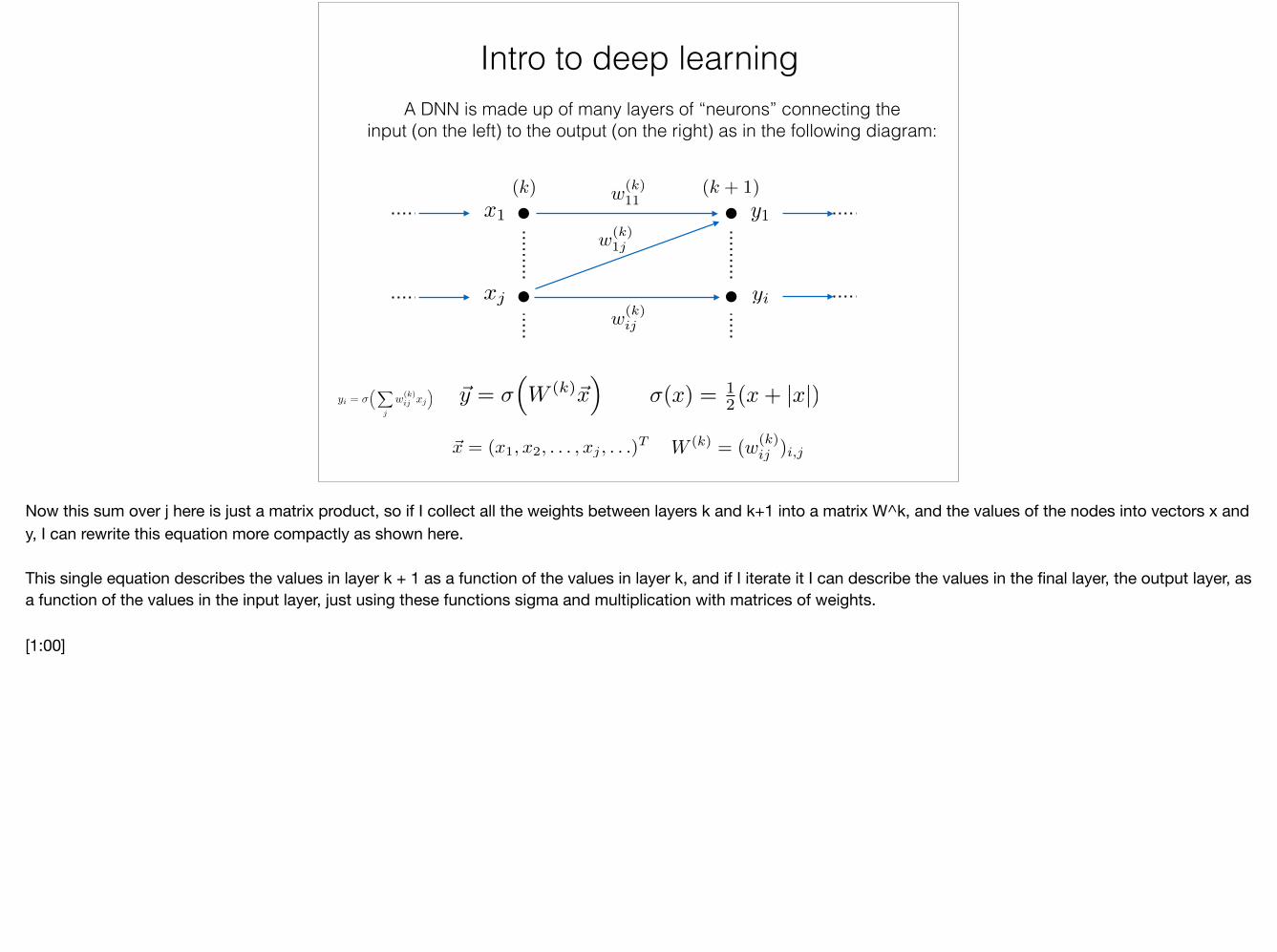
Now this sum over j here is just a matrix product, so if I collect all the weights between layers k and k+1 into a matrix W^k, and the values of the nodes into vectors x and y, I can rewrite this equation more compactly as shown here.

This single equation describes the values in layer k + 1 as a function of the values in layer k, and if I iterate it I can describe the values in the final layer, the output layer, as a function of the values in the input layer, just using these functions sigma and multiplication with matrices of weights.

[1:00]


(0) (L+ 1)x1

xj

Fw : Rm �! Rn


Fw(~x) = �

⇣W

(L) · · ·�⇣W

(1)�

⇣W

(0)~x

⌘· · ·

⌘

xm

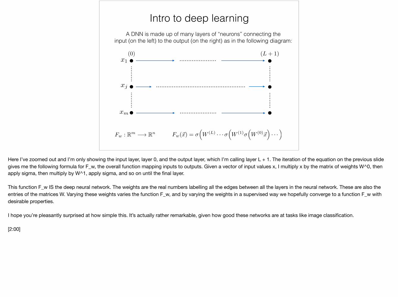
Here I’ve zoomed out and I’m only showing the input layer, layer 0, and the output layer, which I’m calling layer L + 1. The iteration of the equation on the previous slide gives me the following formula for F_w, the overall function mapping inputs to outputs. Given a vector of input values x, I multiply x by the matrix of weights W^0, then apply sigma, then multiply by W^1, apply sigma, and so on until the final layer.

This function F_w IS the deep neural network. The weights are the real numbers labelling all the edges between all the layers in the neural network. These are also the entries of the matrices W. Varying these weights varies the function F_w, and by varying the weights in a supervised way we hopefully converge to a function F_w with desirable properties.

I hope you’re pleasantly surprised at how simple this. It’s actually rather remarkable, given how good these networks are at tasks like image classification.

[2:00]

• Natural Language Processing (NLP) includes machine translation, processing of natural language queries (e.g. Siri) and question answering wrt. unstructured text (e.g. “where is the ring at the end of LoTR?”).

• Two common neural network architectures for NLP are Recurrent Neural Networks (RNN) and Long-Short Term Memory (LSTM). Both are variations on the DNN architecture.

• Many hard unsolved NLP problems require sophisticated reasoning about context and an understanding of algorithms. To solve these problems, recent work equips RNNs/LSTMs with “Von Neumann elements” e.g. stack memory.

• RNN/LSTM controllers + differentiable memory is one model of differentiable programming, currently being explored at e.g. Google, Facebook, …

Applied deep learning

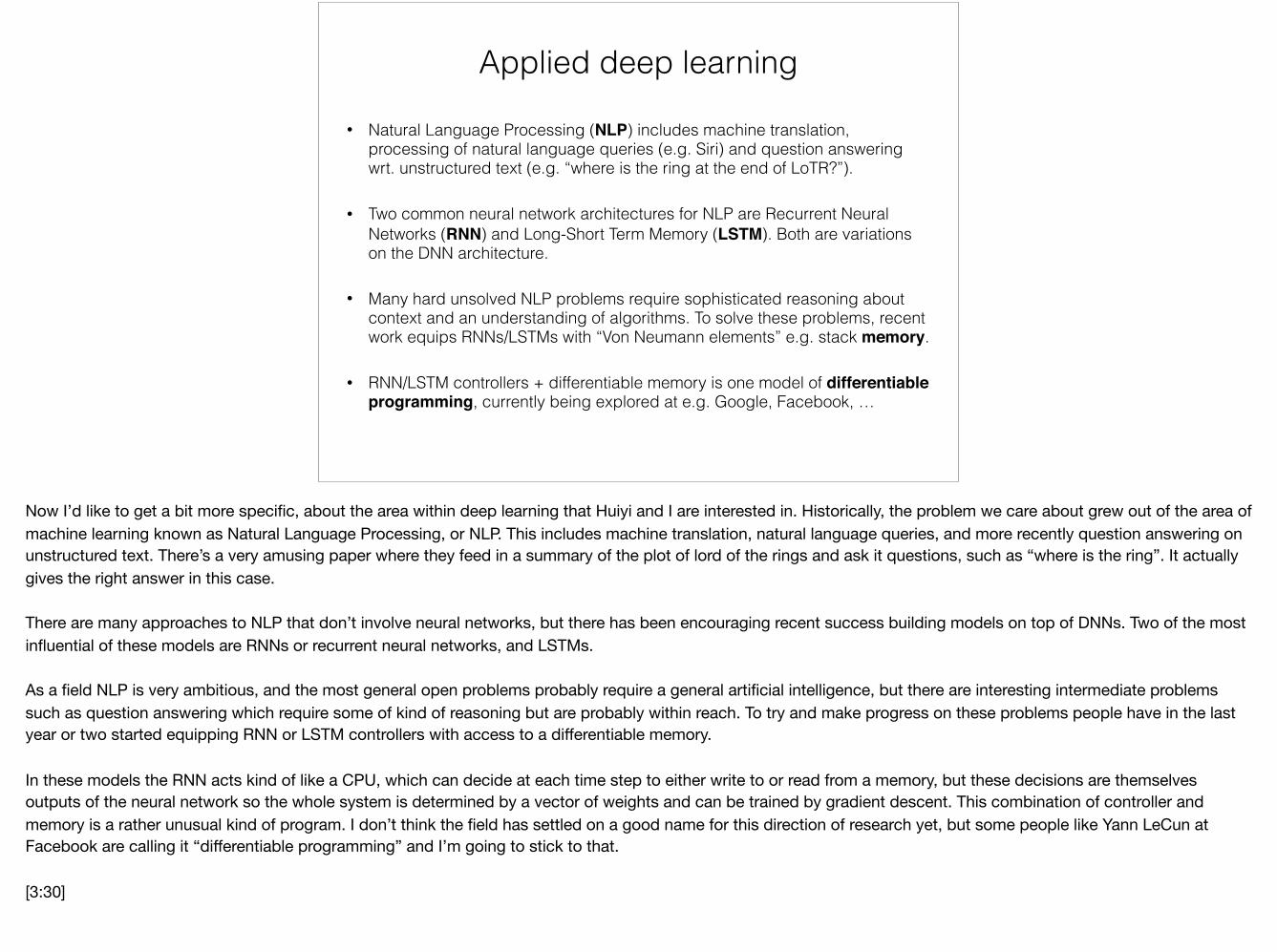
Now I’d like to get a bit more specific, about the area within deep learning that Huiyi and I are interested in. Historically, the problem we care about grew out of the area of machine learning known as Natural Language Processing, or NLP. This includes machine translation, natural language queries, and more recently question answering on unstructured text. There’s a very amusing paper where they feed in a summary of the plot of lord of the rings and ask it questions, such as “where is the ring”. It actually gives the right answer in this case.

There are many approaches to NLP that don’t involve neural networks, but there has been encouraging recent success building models on top of DNNs. Two of the most influential of these models are RNNs or recurrent neural networks, and LSTMs.

As a field NLP is very ambitious, and the most general open problems probably require a general artificial intelligence, but there are interesting intermediate problems such as question answering which require some of kind of reasoning but are probably within reach. To try and make progress on these problems people have in the last year or two started equipping RNN or LSTM controllers with access to a differentiable memory.

In these models the RNN acts kind of like a CPU, which can decide at each time step to either write to or read from a memory, but these decisions are themselves outputs of the neural network so the whole system is determined by a vector of weights and can be trained by gradient descent. This combination of controller and memory is a rather unusual kind of program. I don’t think the field has settled on a good name for this direction of research yet, but some people like Yann LeCun at Facebook are calling it “differentiable programming” and I’m going to stick to that.

[3:30]

• These “memory enhanced” neural networks are already being used in production, e.g. Facebook messenger (~900m users).

Salon, “Facebook Thinks It Has Found the Secret to Making Bots Less Dumb”, June 28 2016.

To give you some idea of how seriously Facebook in particular is taking this research, I’ve put here an extract from an article I just happened to see yesterday on salon.com. Apparently these memory-enhanced neural networks are already in a beta form of Facebook’s messenger app, as part of their new commerce bot features. So this stuff really works, at least in some narrow domains.

[2:00]

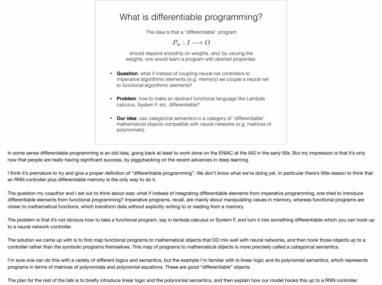
What is differentiable programming?

• Question: what if instead of coupling neural net controllers to imperative algorithmic elements (e.g. memory) we couple a neural net to functional algorithmic elements?

• Problem: how to make an abstract functional language like Lambda calculus, System F, etc. differentiable?

• Our idea: use categorical semantics in a category of “differentiable” mathematical objects compatible with neural networks (e.g. matrices of polynomials).

The idea is that a “differentiable” program

Pw : I �! O

should depend smoothly on weights, and, by varying the weights, one would learn a program with desired properties.

In some sense differentiable programming is an old idea, going back at least to work done on the ENIAC at the IAS in the early 50s. But my impression is that it’s only now that people are really having significant success, by piggybacking on the recent advances in deep learning.

I think it’s premature to try and give a proper definition of “differentiable programming”. We don’t know what we’re doing yet. In particular there’s little reason to think that an RNN controller plus differentiable memory is the only way to do it.

The question my coauthor and I set out to think about was: what if instead of integrating differentiable elements from imperative programming, one tried to introduce differentiable elements from functional programming? Imperative programs, recall, are mainly about manipulating values in memory, whereas functional programs are closer to mathematical functions, which transform data without explicitly writing to or reading from a memory.

The problem is that it’s not obvious how to take a functional program, say in lambda calculus or System F, and turn it into something differentiable which you can hook up to a neural network controller.

The solution we came up with is to first map functional programs to mathematical objects that DO mix well with neural networks, and then hook those objects up to a controller rather than the symbolic programs themselves. This map of programs to mathematical objects is more precisely called a categorical semantics.

I’m sure one can do this with a variety of different logics and semantics, but the example I’m familiar with is linear logic and its polynomial semantics, which represents programs in terms of matrices of polynomials and polynomial equations. These are good “differentiable” objects.

The plan for the rest of the talk is to briefly introduce linear logic and the polynomial semantics, and then explain how our model hooks this up to a RNN controller.

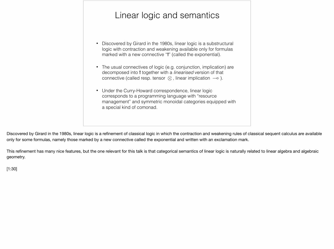
• Discovered by Girard in the 1980s, linear logic is a substructural logic with contraction and weakening available only for formulas marked with a new connective “!” (called the exponential).

• The usual connectives of logic (e.g. conjunction, implication) are decomposed into ! together with a linearised version of that connective (called resp. tensor , linear implication ).

• Under the Curry-Howard correspondence, linear logic corresponds to a programming language with “resource management” and symmetric monoidal categories equipped with a special kind of comonad.

Linear logic and semantics

⌦ (

Discovered by Girard in the 1980s, linear logic is a refinement of classical logic in which the contraction and weakening rules of classical sequent calculus are available only for some formulas, namely those marked by a new connective called the exponential and written with an exclamation mark.

This refinement has many nice features, but the one relevant for this talk is that categorical semantics of linear logic is naturally related to linear algebra and algebraic geometry.

[1:30]

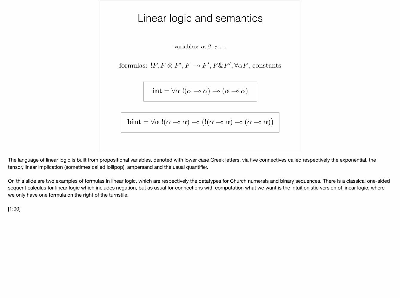
variables: ↵,�, �, . . .

bint = 8↵ !(↵ ( ↵) (�!(↵ ( ↵) ( (↵ ( ↵)

�

int = 8↵ !(↵ ( ↵) ( (↵ ( ↵)

formulas: !F, F ⌦ F 0, F ( F 0, F&F 0, 8↵F , constants

Linear logic and semantics

The language of linear logic is built from propositional variables, denoted with lower case Greek letters, via five connectives called respectively the exponential, the tensor, linear implication (sometimes called lollipop), ampersand and the usual quantifier.

On this slide are two examples of formulas in linear logic, which are respectively the datatypes for Church numerals and binary sequences. There is a classical one-sided sequent calculus for linear logic which includes negation, but as usual for connections with computation what we want is the intuitionistic version of linear logic, where we only have one formula on the right of the turnstile.

[1:00]

More precisely, let us define a pre-proof to be a rooted tree whose edges are labelledwith sequents. In order to follow the logical ordering, the tree is presented with its rootvertex (the sequent to be proven) at the bottom of the page, and we orient edges towardsthe root (so downwards). The labels on incoming edges at a vertex are called hypothesesand on the outgoing edge the conclusion. For example consider the following tree, and itsequivalent presentation in sequent calculus notation:

� ` A � ` B

�,� ` A⌦ B

� ` A � ` B

�,� ` A⌦ B

Leaves are presented in the sequent calculus notation with an empty numerator.

Definition 4.1.A proof is a pre-proof together with a compatible labelling of vertices bydeduction rules. The list of deduction rules is given in the first column of (4.2) – (4.14).A labelling is compatible if at each vertex, the sequents labelling the incident edges matchthe format displayed in the deduction rule.

In all deduction rules, the sets � and�may be empty and, in particular, the promotionrule may be used with an empty premise. In the promotion rule, !� stands for a list offormulas each of which is preceeded by an exponential modality, for example !A1, . . . , !An

.The diagrams on the right are string diagrams and should be ignored until Section 5. Inparticular they are not the trees associated to proofs.

(Axiom):A ` A

A

A

(4.2)

�, A,B,� ` C

(Exchange):�, B,A,� ` C

� AB �

C

(4.3)

8

More precisely, let us define a pre-proof to be a rooted tree whose edges are labelledwith sequents. In order to follow the logical ordering, the tree is presented with its rootvertex (the sequent to be proven) at the bottom of the page, and we orient edges towardsthe root (so downwards). The labels on incoming edges at a vertex are called hypothesesand on the outgoing edge the conclusion. For example consider the following tree, and itsequivalent presentation in sequent calculus notation:

� ` A � ` B

�,� ` A⌦ B

� ` A � ` B

�,� ` A⌦ B

Leaves are presented in the sequent calculus notation with an empty numerator.

Definition 4.1.A proof is a pre-proof together with a compatible labelling of vertices bydeduction rules. The list of deduction rules is given in the first column of (4.2) – (4.14).A labelling is compatible if at each vertex, the sequents labelling the incident edges matchthe format displayed in the deduction rule.

In all deduction rules, the sets � and�may be empty and, in particular, the promotionrule may be used with an empty premise. In the promotion rule, !� stands for a list offormulas each of which is preceeded by an exponential modality, for example !A1, . . . , !An

.The diagrams on the right are string diagrams and should be ignored until Section 5. Inparticular they are not the trees associated to proofs.

(Axiom):A ` A

A

A

(4.2)

�, A,B,� ` C

(Exchange):�, B,A,� ` C

� AB �

C

(4.3)

8

� ` A �0, A,� ` B

(Cut): cut�0

,�,� ` B

B

� ��0

A (4.4)

� ` A � ` B(Right ⌦): ⌦-R�,� ` A⌦ B

A B

� �

(4.5)

�, A,B,� ` C

(Left ⌦): ⌦-L�, A⌦ B,� ` C

� A⌦ B �

C

(4.6)

A,� ` B

(Right (): ( R

� ` A ( B

A ( B

�

A

B

(4.7)

9

� ` A �0, A,� ` B

(Cut): cut�0

,�,� ` B

B

� ��0

A (4.4)

� ` A � ` B(Right ⌦): ⌦-R�,� ` A⌦ B

A B

� �

(4.5)

�, A,B,� ` C

(Left ⌦): ⌦-L�, A⌦ B,� ` C

� A⌦ B �

C

(4.6)

A,� ` B

(Right (): ( R

� ` A ( B

A ( B

�

A

B

(4.7)

9

� ` A �0, A,� ` B

(Cut): cut�0

,�,� ` B

B

� ��0

A (4.4)

� ` A � ` B(Right ⌦): ⌦-R�,� ` A⌦ B

A B

� �

(4.5)

�, A,B,� ` C

(Left ⌦): ⌦-L�, A⌦ B,� ` C

� A⌦ B �

C

(4.6)

A,� ` B

(Right (): ( R

� ` A ( B

A ( B

�

A

B

(4.7)

9

� ` A �0, A,� ` B

(Cut): cut�0

,�,� ` B

B

� ��0

A (4.4)

� ` A � ` B(Right ⌦): ⌦-R�,� ` A⌦ B

A B

� �

(4.5)

�, A,B,� ` C

(Left ⌦): ⌦-L�, A⌦ B,� ` C

� A⌦ B �

C

(4.6)

A,� ` B

(Right (): ( R

� ` A ( B

A ( B

�

A

B

(4.7)

9

� ` A �0, B,� ` C

(Left (): ( L

�0,�, A ( B,� ` C

C

��0 � A ( B

B

A (4.8)

!� ` A(Promotion): prom!� `!A

!A

!�

A

(4.9)

�, A,� ` B

(Dereliction): der�, !A,� ` B

B

� �!A

A (4.10)

�, !A, !A,� ` B

(Contraction): ctr�, !A,� ` B

B

� �!A

(4.11)

10

� ` A �0, B,� ` C

(Left (): ( L

�0,�, A ( B,� ` C

C

��0 � A ( B

B

A (4.8)


!A

!�

A

(4.9)

�, A,� ` B


B

� �!A

A (4.10)

�, !A, !A,� ` B


B

� �!A

(4.11)

10

� ` A �0, B,� ` C

(Left (): ( L

�0,�, A ( B,� ` C

C

��0 � A ( B

B

A (4.8)


!A

!�

A

(4.9)

�, A,� ` B


B

� �!A

A (4.10)

�, !A, !A,� ` B


B

� �!A

(4.11)

10

� ` A �0, B,� ` C

(Left (): ( L

�0,�, A ( B,� ` C

C

��0 � A ( B

B

A (4.8)


!A

!�

A

(4.9)

�, A,� ` B


B

� �!A

A (4.10)

�, !A, !A,� ` B


B

� �!A

(4.11)

10

�,� ` B

(Weakening): weak�, !A,� ` B

B

� �!A

(4.12)

�,� ` A

(Left 1): 1-L�, 1,� ` A

B

� �1

(4.13)

(Right 1): 1-R` 1

1

1(4.14)

Example 4.2.For any formula A let 2A

denote the proof (2.4) from Section 2, which werepeat here for the reader’s convenience:

A ` A

A ` A A ` A ( L

A,A ( A ` A

( L

A,A ( A,A ( A ` A

( R

A ( A,A ( A ` A ( A

der!(A ( A), A ( A ` A ( A

der!(A ( A), !(A ( A) ` A (

ctr!(A ( A) ` A ( A

( R

` intA

(4.15)

We also write 2A

for the proof of !(A ( A) ` A ( A obtained by reading the above proofup to the penultimate line. For each integer n � 0 there is a proof n

A

of intA

constructedalong similar lines, see [22, §5.3.2] and [15, §3.1].

In what sense is this proof an avatar of the number 2? In the context of the �-calculuswe appreciated the relationship between the term T and the number 2 only after we sawhow T interacted with other terms M by forming the function application (T M) andthen finding a normal form with respect to �-equivalence.

The analogue of function application in linear logic is the cut rule. The analogue of�-equivalence is an equivalence relation on the set of proofs of any sequent, which we write

11

Definition 7.5 (Second-order linear logic).The formulas of second-order linear logicare defined recursively as follows: any formula of propositional linear logic is a formula,and if A is a formula then so is 8x .A for any propositional variable x. There are two newdeduction rules:

� ` A 8R� ` 8x .A

�, A[B/x] ` C

8L�, 8x .A ` C

where � is a sequence of formulas, possibly empty, and in the right introduction rule werequire that x is not free in any formula of �. Here A[B/x] means a formula A with allfree occurrences of x replaced by a formula B (as usual, there is some chicanery necessaryto avoid free variables in B being captured, but we ignore this).

Intuitively, the right introduction rule takes a proof ⇡ and “exposes” the variable x,for which any type may be substituted. The left introduction rule, dually, takes a formulaB in some proof and binds it to a variable x. The result of cutting a right introductionrule against a left introduction rule is that the formula B will be bound to x throughoutthe proof ⇡. That is, cut-elimination transforms

⇡

.

.

.

� ` A

8R� ` 8x .A

⇢

.

.

.

�, A[B/x] ` C

8L�, 8x .A ` C

cut

�,� ` C

(7.8)

to the proof

⇡[B/x]

.

.

.

� ` A[B/x]

⇢

.

.

.

�, A[B/x] ` C

cut

�,� ` C

(7.9)

where ⇡[B/x] denotes the result of replacing all occurrences of x in the proof ⇡ with B. Inthe remainder of this section we provide a taste of just what an explosion of possibilitiesthe addition of quantifiers to the language represents.

Example 7.6 (Integers).The type of integers is

int = 8x . !(x ( x) ( (x ( x) .

For each integer n � 0 we define n to be the proof

32

Definition 7.5 (Second-order linear logic).The formulas of second-order linear logicare defined recursively as follows: any formula of propositional linear logic is a formula,and if A is a formula then so is 8x .A for any propositional variable x. There are two newdeduction rules:

� ` A 8R� ` 8x .A

�, A[B/x] ` C

8L�, 8x .A ` C

where � is a sequence of formulas, possibly empty, and in the right introduction rule werequire that x is not free in any formula of �. Here A[B/x] means a formula A with allfree occurrences of x replaced by a formula B (as usual, there is some chicanery necessaryto avoid free variables in B being captured, but we ignore this).

Intuitively, the right introduction rule takes a proof ⇡ and “exposes” the variable x,for which any type may be substituted. The left introduction rule, dually, takes a formulaB in some proof and binds it to a variable x. The result of cutting a right introductionrule against a left introduction rule is that the formula B will be bound to x throughoutthe proof ⇡. That is, cut-elimination transforms

⇡

.

.

.

� ` A

8R� ` 8x .A

⇢

.

.

.

�, A[B/x] ` C

8L�, 8x .A ` C

cut

�,� ` C

(7.8)

to the proof

⇡[B/x]

.

.

.

� ` A[B/x]

⇢

.

.

.

�, A[B/x] ` C

cut

�,� ` C

(7.9)

where ⇡[B/x] denotes the result of replacing all occurrences of x in the proof ⇡ with B. Inthe remainder of this section we provide a taste of just what an explosion of possibilitiesthe addition of quantifiers to the language represents.

Example 7.6 (Integers).The type of integers is

int = 8x . !(x ( x) ( (x ( x) .

For each integer n � 0 we define n to be the proof

32

Deduction rules for linear logic

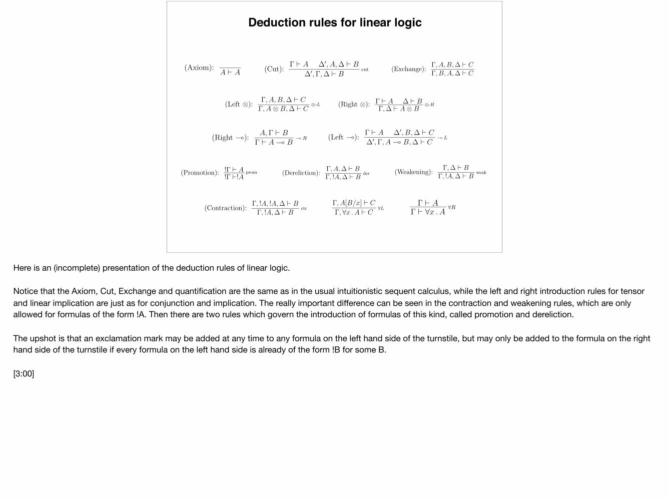
Here is an (incomplete) presentation of the deduction rules of linear logic.

Notice that the Axiom, Cut, Exchange and quantification are the same as in the usual intuitionistic sequent calculus, while the left and right introduction rules for tensor and linear implication are just as for conjunction and implication. The really important difference can be seen in the contraction and weakening rules, which are only allowed for formulas of the form !A. Then there are two rules which govern the introduction of formulas of this kind, called promotion and dereliction.

The upshot is that an exclamation mark may be added at any time to any formula on the left hand side of the turnstile, but may only be added to the formula on the right hand side of the turnstile if every formula on the left hand side is already of the form !B for some B.

[3:00]

Binary integers

S 2 {0, 1}⇤ 7�! proof tS of ` bint

bint = 8↵ !(↵ ( ↵) (�!(↵ ( ↵) ( (↵ ( ↵)

�

t001

↵ ` ↵

↵ ` ↵↵ ` ↵ ↵ ` ↵ ( L↵,↵ ( ↵ ` ↵

( L↵,↵ ( ↵,↵ ( ↵ ` ↵

( L↵,↵ ( ↵,↵ ( ↵,↵ ( ↵ ` ↵

( R↵ ( ↵,↵ ( ↵,↵ ( ↵ ` ↵ ( ↵

der!(↵ ( ↵), !(↵ ( ↵), !(↵ ( ↵) ` ↵ ( ↵

ctr!(↵ ( ↵), !(↵ ( ↵) ` ↵ ( ↵

( R!(↵ ( ↵) ` !(↵ ( ↵) ( (↵ ( ↵)

( R` !(↵ ( ↵) (

�!(↵ ( ↵) ( (↵ ( ↵)

�

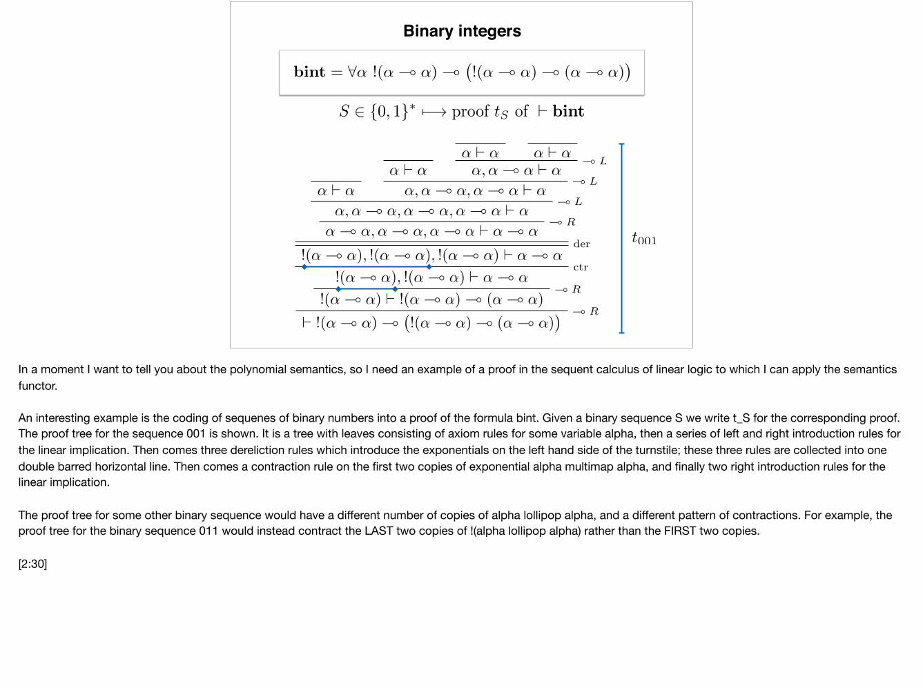
In a moment I want to tell you about the polynomial semantics, so I need an example of a proof in the sequent calculus of linear logic to which I can apply the semantics functor.

An interesting example is the coding of sequenes of binary numbers into a proof of the formula bint. Given a binary sequence S we write t_S for the corresponding proof. The proof tree for the sequence 001 is shown. It is a tree with leaves consisting of axiom rules for some variable alpha, then a series of left and right introduction rules for the linear implication. Then comes three dereliction rules which introduce the exponentials on the left hand side of the turnstile; these three rules are collected into one double barred horizontal line. Then comes a contraction rule on the first two copies of exponential alpha multimap alpha, and finally two right introduction rules for the linear implication.

The proof tree for some other binary sequence would have a different number of copies of alpha lollipop alpha, and a different pattern of contractions. For example, the proof tree for the binary sequence 011 would instead contract the LAST two copies of !(alpha lollipop alpha) rather than the FIRST two copies.

[2:30]

(one variable per entry in a d x d matrix)

Polynomial semantics (sketch)

J↵K = Rd

J↵ ( ↵K = L(Rd,Rd) = Md(R)

J!(↵ ( ↵)K = R[{aij}1i,jd] = R[a11, . . . , aij , . . . , add]

JbintK = J!(↵ ( ↵) (�!(↵ ( ↵) ( (↵ ( ↵)

�K

= Md

�R[{aij , a0ij}1i,jd]

�

(matrices of polynomials in the variables a, a’)

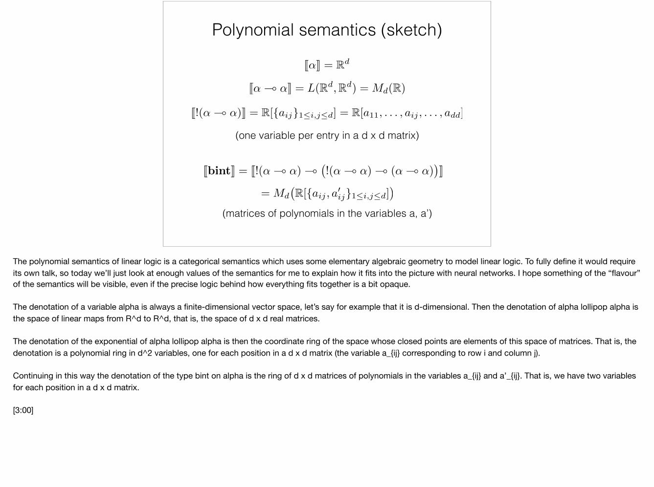
The polynomial semantics of linear logic is a categorical semantics which uses some elementary algebraic geometry to model linear logic. To fully define it would require its own talk, so today we’ll just look at enough values of the semantics for me to explain how it fits into the picture with neural networks. I hope something of the “flavour” of the semantics will be visible, even if the precise logic behind how everything fits together is a bit opaque.

The denotation of a variable alpha is always a finite-dimensional vector space, let’s say for example that it is d-dimensional. Then the denotation of alpha lollipop alpha is the space of linear maps from R^d to R^d, that is, the space of d x d real matrices.

The denotation of the exponential of alpha lollipop alpha is then the coordinate ring of the space whose closed points are elements of this space of matrices. That is, the denotation is a polynomial ring in d^2 variables, one for each position in a d x d matrix (the variable a_{ij} corresponding to row i and column j).

Continuing in this way the denotation of the type bint on alpha is the ring of d x d matrices of polynomials in the variables a_{ij} and a’_{ij}. That is, we have two variables for each position in a d x d matrix.

[3:00]


JbintK = Md


�

tS : bint, JtSK 2 JbintK

Jt0K =

0

BBB@

a11 · · · a1da21 · · · a2d...

...ad1 · · · add

1

CCCAJt1K =

0

BBB@

a011 · · · a01da021 · · · a02d...

...a0d1 · · · a0dd

1

CCCA

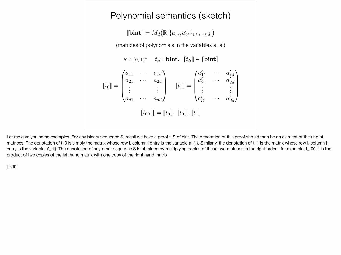
Jt001K = Jt0K · Jt0K · Jt1K


S 2 {0, 1}⇤

Let me give you some examples. For any binary sequence S, recall we have a proof t_S of bint. The denotation of this proof should then be an element of the ring of matrices. The denotation of t_0 is simply the matrix whose row i, column j entry is the variable a_{ij}. Similarly, the denotation of t_1 is the matrix whose row i, column j entry is the variable a’_{ij}. The denotation of any other sequence S is obtained by multiplying copies of these two matrices in the right order - for example, t_{001} is the product of two copies of the left hand matrix with one copy of the right hand matrix.

[1:30]


JbintK = Md


�

tS : bint, JtSK 2 JbintK


vector space

Jt0KJt1K

Jt001K

JbintK

Upshot: proofs/programs to vectors

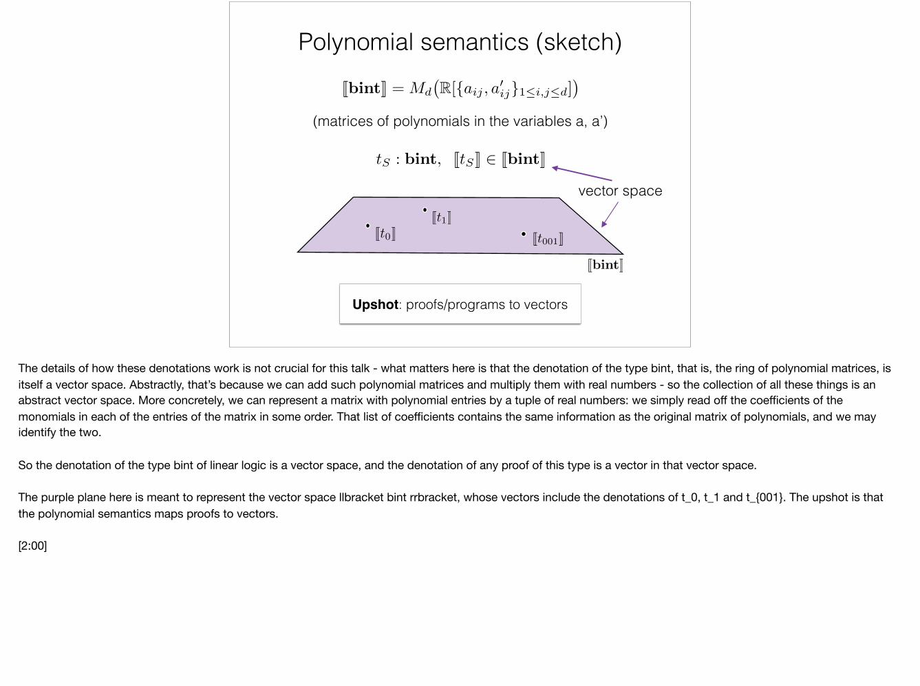
The details of how these denotations work is not crucial for this talk - what matters here is that the denotation of the type bint, that is, the ring of polynomial matrices, is itself a vector space. Abstractly, that’s because we can add such polynomial matrices and multiply them with real numbers - so the collection of all these things is an abstract vector space. More concretely, we can represent a matrix with polynomial entries by a tuple of real numbers: we simply read off the coefficients of the monomials in each of the entries of the matrix in some order. That list of coefficients contains the same information as the original matrix of polynomials, and we may identify the two.

So the denotation of the type bint of linear logic is a vector space, and the denotation of any proof of this type is a vector in that vector space.

The purple plane here is meant to represent the vector space llbracket bint rrbracket, whose vectors include the denotations of t_0, t_1 and t_{001}. The upshot is that the polynomial semantics maps proofs to vectors.

[2:00]


JbintK = Md


�


Jt0KJt1K

Jt001K

JbintK


T

T 2

evalT (A,B) = T |aij=Aij ,a0ij=Bij A,B 2 Md(R)

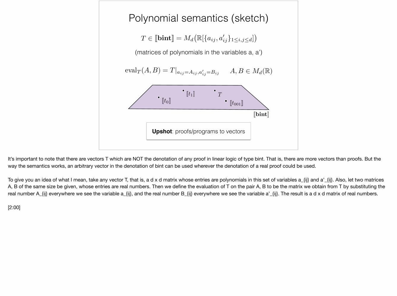
It’s important to note that there are vectors T which are NOT the denotation of any proof in linear logic of type bint. That is, there are more vectors than proofs. But the way the semantics works, an arbitrary vector in the denotation of bint can be used wherever the denotation of a real proof could be used.

To give you an idea of what I mean, take any vector T, that is, a d x d matrix whose entries are polynomials in this set of variables a_{ij} and a’_{ij}. Also, let two matrices A, B of the same size be given, whose entries are real numbers. Then we define the evaluation of T on the pair A, B to be the matrix we obtain from T by substituting the real number A_{ij} everywhere we see the variable a_{ij}, and the real number B_{ij} everywhere we see the variable a’_{ij}. The result is a d x d matrix of real numbers.

[2:00]


JbintK = Md


�


Jt0KJt1K

Jt001K

JbintK


T

T 2

evalJt0K(A,B) = A evalJt001K(A,B) = AAB

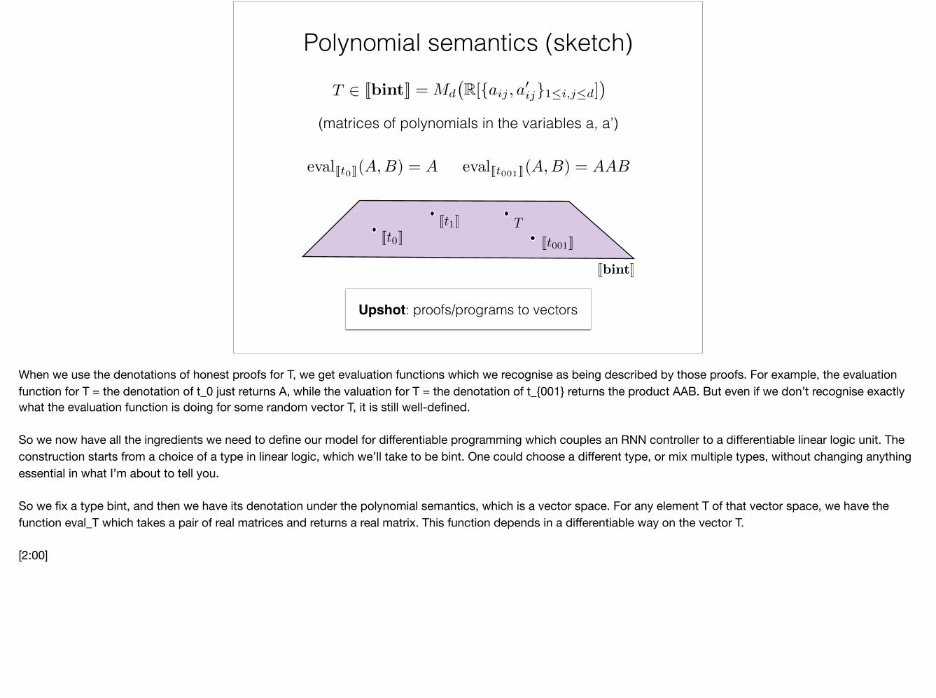
When we use the denotations of honest proofs for T, we get evaluation functions which we recognise as being described by those proofs. For example, the evaluation function for T = the denotation of t_0 just returns A, while the valuation for T = the denotation of t_{001} returns the product AAB. But even if we don’t recognise exactly what the evaluation function is doing for some random vector T, it is still well-defined.

So we now have all the ingredients we need to define our model for differentiable programming which couples an RNN controller to a differentiable linear logic unit. The construction starts from a choice of a type in linear logic, which we’ll take to be bint. One could choose a different type, or mix multiple types, without changing anything essential in what I’m about to tell you.

So we fix a type bint, and then we have its denotation under the polynomial semantics, which is a vector space. For any element T of that vector space, we have the function eval_T which takes a pair of real matrices and returns a real matrix. This function depends in a differentiable way on the vector T.

[2:00]

Our model: RNN controller + differentiable “linear logic” moduleH

tit'

-hit)

• •

AH) •

•QA 7 i S

)•

.. . > : eval ,H( ATMBH) ,

: > " '

; QB•

;

• -'

i BY -

•

QT U-1 9. Tlt ) •

• :

;Ct )

hlt ' - 6(SevaltH( AM,

BM ) +

Hhlt'

't UXH )

AlH= 6( Qah't ' ' ' )

BH = 6 ( Qpsh 't ' ' ' )TH = 6 ( Qththt )

H,S, U,QA, QB , QT are matrices of weights

h(t) = �⇣S evalT (t)(A(t), B(t)) +Hh(t�1) + Ux(t)

⌘

A(t) = �⇣QAh

(t�1)⌘

B(t) = �⇣QBh

(t�1)⌘

T (t) = �⇣QTh

(t�1)⌘

T (t) 2 JbintK

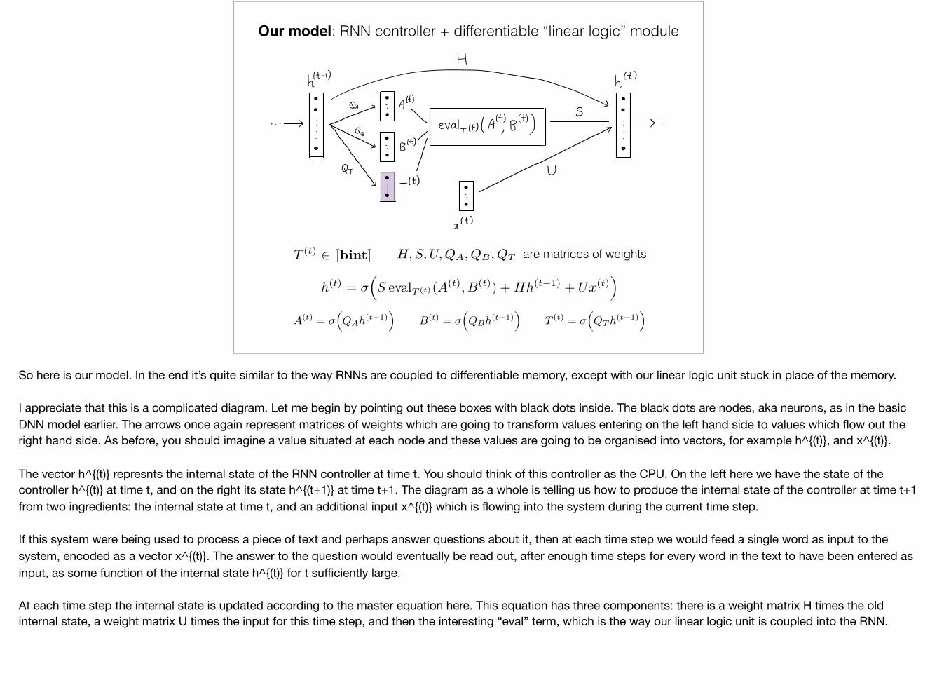
So here is our model. In the end it’s quite similar to the way RNNs are coupled to differentiable memory, except with our linear logic unit stuck in place of the memory.

I appreciate that this is a complicated diagram. Let me begin by pointing out these boxes with black dots inside. The black dots are nodes, aka neurons, as in the basic DNN model earlier. The arrows once again represent matrices of weights which are going to transform values entering on the left hand side to values which flow out the right hand side. As before, you should imagine a value situated at each node and these values are going to be organised into vectors, for example h^{(t)}, and x^{(t)}.

The vector h^{(t)} represnts the internal state of the RNN controller at time t. You should think of this controller as the CPU. On the left here we have the state of the controller h^{(t)} at time t, and on the right its state h^{(t+1)} at time t+1. The diagram as a whole is telling us how to produce the internal state of the controller at time t+1 from two ingredients: the internal state at time t, and an additional input x^{(t)} which is flowing into the system during the current time step.

If this system were being used to process a piece of text and perhaps answer questions about it, then at each time step we would feed a single word as input to the system, encoded as a vector x^{(t)}. The answer to the question would eventually be read out, after enough time steps for every word in the text to have been entered as input, as some function of the internal state h^{(t)} for t sufficiently large.

At each time step the internal state is updated according to the master equation here. This equation has three components: there is a weight matrix H times the old internal state, a weight matrix U times the input for this time step, and then the interesting “eval” term, which is the way our linear logic unit is coupled into the RNN.

Our model: RNN controller + differentiable “linear logic” moduleH

tit'

-hit)

• •

AH) •

•QA 7 i S

)•

.. . > : eval ,H( ATMBH) ,

: > " '

; QB•

;

• -'

i BY -

•

QT U-1 9. Tlt ) •

• :

;Ct )

hlt ' - 6(SevaltH( AM,

BM ) +

Hhlt'

't UXH )

AlH= 6( Qah't ' ' ' )

BH = 6 ( Qpsh 't ' ' ' )TH = 6 ( Qththt )

H,S, U,QA, QB , QT are matrices of weights

h(t) = �⇣S evalT (t)(A(t), B(t)) +Hh(t�1) + Ux(t)

⌘

A(t) = �⇣QAh

(t�1)⌘

B(t) = �⇣QBh

(t�1)⌘

T (t) = �⇣QTh

(t�1)⌘

T (t) 2 JbintK

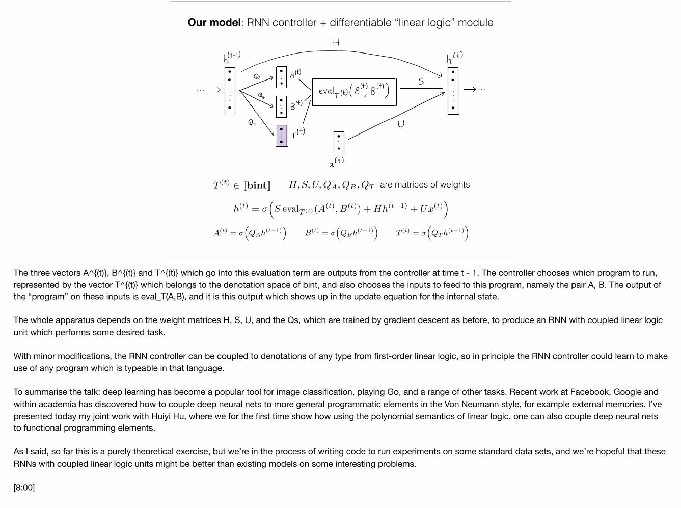
The three vectors A^{(t)}, B^{(t)} and T^{(t)} which go into this evaluation term are outputs from the controller at time t - 1. The controller chooses which program to run, represented by the vector T^{(t)} which belongs to the denotation space of bint, and also chooses the inputs to feed to this program, namely the pair A, B. The output of the “program” on these inputs is eval_T(A,B), and it is this output which shows up in the update equation for the internal state.

The whole apparatus depends on the weight matrices H, S, U, and the Qs, which are trained by gradient descent as before, to produce an RNN with coupled linear logic unit which performs some desired task.

With minor modifications, the RNN controller can be coupled to denotations of any type from first-order linear logic, so in principle the RNN controller could learn to make use of any program which is typeable in that language.

To summarise the talk: deep learning has become a popular tool for image classification, playing Go, and a range of other tasks. Recent work at Facebook, Google and within academia has discovered how to couple deep neural nets to more general programmatic elements in the Von Neumann style, for example external memories. I’ve presented today my joint work with Huiyi Hu, where we for the first time show how using the polynomial semantics of linear logic, one can also couple deep neural nets to functional programming elements.

As I said, so far this is a purely theoretical exercise, but we’re in the process of writing code to run experiments on some standard data sets, and we’re hopeful that these RNNs with coupled linear logic units might be better than existing models on some interesting problems.

[8:00]

Linear logic and deep learning - The Rising Seatherisingsea.org/notes/talk-lldl-transcript.pdf ·...

Documents

Transcript of Linear logic and deep learning - The Rising Seatherisingsea.org/notes/talk-lldl-transcript.pdf ·...