Linear Discriminant Functions 主講人:虞台文. Contents Introduction Linear Discriminant...
56
Linear Discriminant Func tions 主主主 主主主 :
-
Upload
justina-foster -
Category
Documents
-
view
243 -
download
8
Transcript of Linear Discriminant Functions 主講人:虞台文. Contents Introduction Linear Discriminant...
Linear Discriminant Functions
主講人:虞台文
Contents
Introduction Linear Discriminant Functions and Decision
Surface Linear Separability Learning
– Gradient Decent Algorithm– Newton’s Method
Linear Discriminant Functions
Introduction
Decision-Making Approaches
Probabilistic Approaches– Based on the underlying probability densities of tr
aining sets.– For example, Bayesian decision rule assumes tha
t the underlying probability densities were available.
Discriminating Approaches– Assume we know the proper forms for the discrimi
nant functions were known.– Use the samples to estimate the values of param
eters of the classifier.
Linear Discriminating Functions
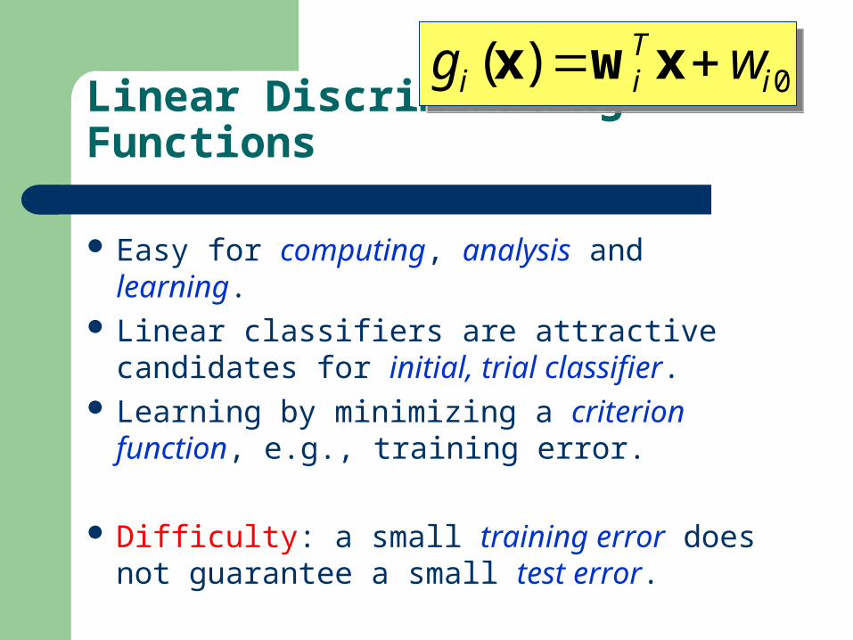
Easy for computing, analysis and learning. Linear classifiers are attractive candidates for
initial, trial classifier. Learning by minimizing a criterion function,
e.g., training error.
Difficulty: a small training error does not guarantee a small test error.
0)( iTii wg xwx 0)( i
Tii wg xwx
Linear Discriminant Functions
Linear Discriminant Functions and Decisi
on Surface
Linear Discriminant Functions
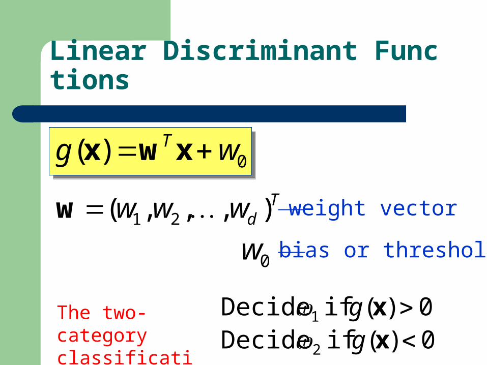
0)( wg T xwx 0)( wg T xwx
Tdwww ),,,( 21 w weight vector
0w bias or threshold
The two-categoryclassification:
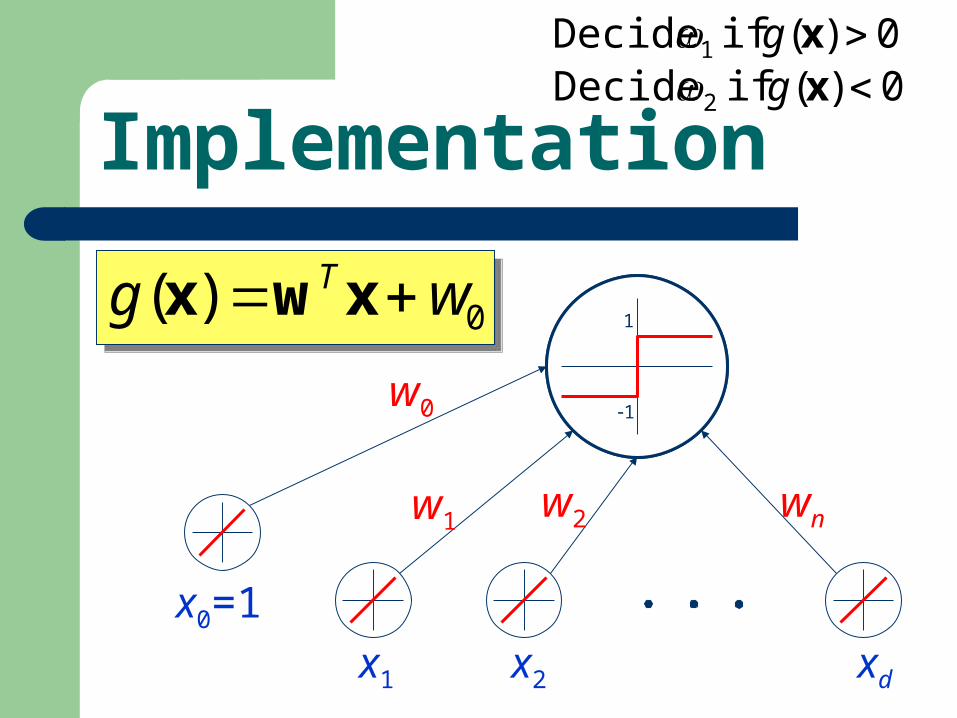
0)( if Decide 1 xg0)( if Decide 2 xg
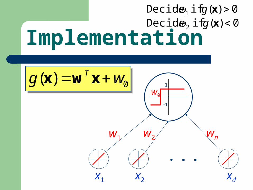
Implementation
0)( wg T xwx 0)( wg T xwxw0
1
1
x1 x2 xd
w1 w2 wn
0)( if Decide 1 xg0)( if Decide 2 xg
Implementation
0)( wg T xwx 0)( wg T xwxw0
1
1
x1 x2 xd
w1 w2 wn
x0=1
w0
1
1
0)( if Decide 1 xg0)( if Decide 2 xg

Decision Surface
0)( wg T xwx 0)( wg T xwx
x1 x2 xd
w1 w2 wn
x0=1
w0
1
1
0)( xg 0)( xg

x1
x2
xn
g(x)=0
Decision Surface
0)( wg T xwx 0)( wg T xwx 0)( xg 0)( xg
x
0||||
)( 02 wg
TT
w
wwxwx
0||||||||
0
w
w
wxw
wT
w w 0/||w
|| 0)( if Decide 1 xg
0)( if Decide 2 xg
1R
2R
x1
x2
xn
g(x)=0
Decision Surface
0)( wg T xwx 0)( wg T xwx
x
w w 0/||w
||1R
2R
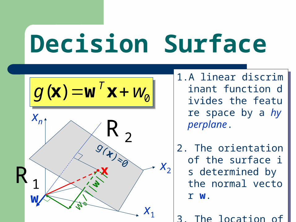
1. A linear discriminant function divides the feature space by a hyperplane.
2. The orientation of the surface is determined by the normal vector w.
3. The location of the surface is determined by the bias w0.
1. A linear discriminant function divides the feature space by a hyperplane.
2. The orientation of the surface is determined by the normal vector w.
3. The location of the surface is determined by the bias w0.
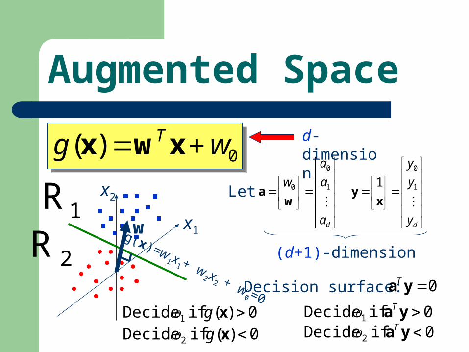
Augmented Space
x1
x2
0)( wg T xwx 0)( wg T xwx
g(x)=w1 x
1 + w2 x
2 + w0 =0
Let
da
a
a
w
1
0
0
wa
dy
y
y
1
0
1
xy
0)( if Decide 1 xg0)( if Decide 2 xg
w
d-dimension
0 if Decide 1 yaT0 if Decide 2 yaT
Decision surface: 0yaT
(d+1)-dimension
1R
2R
Augmented Space
x1
x2
0)( wg T xwx 0)( wg T xwx
g(x)=w1 x
1 + w2 x
2 + w0 =0
Let
da
a
a
w
1
0
0
wa
dy
y
y
1
0
1
xy
0)( if Decide 1 xg0)( if Decide 2 xg
w
d-dimension
0 if Decide 1 yaT0 if Decide 2 yaT
Decision surface: 0yaT
(d+1)-dimension
1R
2R
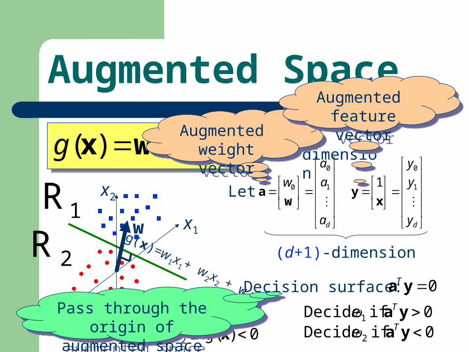
Augmented weight vector
Augmented weight vector
Augmented feature vector
Augmented feature vector
Pass through the origin of augmented space
Pass through the origin of augmented space

Augmented Space
x1
x2
0)( wg T xwx 0)( wg T xwx
g(x)=w1 x
1 + w2 x
2 + w0 =0
w1R
2Ry1
y2
y01
1R
2R
ay = 0
a
Augmented Space
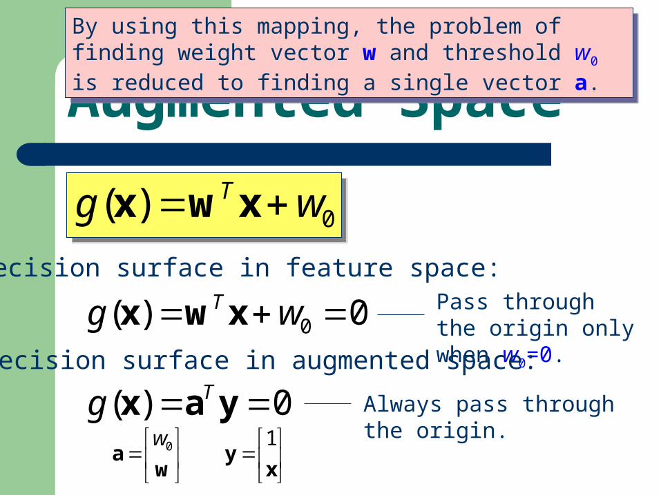
0)( wg T xwx 0)( wg T xwx
Decision surface in feature space:
0)( 0 wg T xwx Pass through the origin only when w0=0.
Decision surface in augmented space:
0)( yax Tg Always pass through the origin.
xy
1
wa 0w
By using this mapping, the problem of finding weight vector w and threshold w0 is reduced to finding a single vector a.
By using this mapping, the problem of finding weight vector w and threshold w0 is reduced to finding a single vector a.
Linear Discriminant Functions
Linear Separability
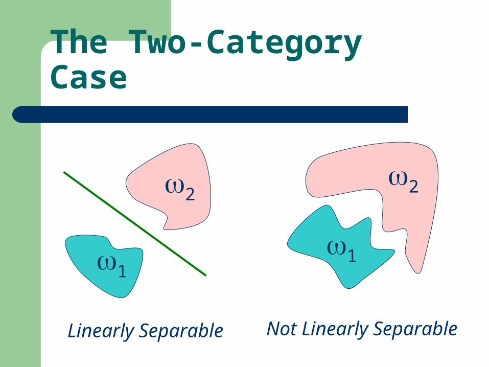
The Two-Category Case
1
2
Linearly Separable
1
2
Not Linearly Separable
The Two-Category Case
1
2
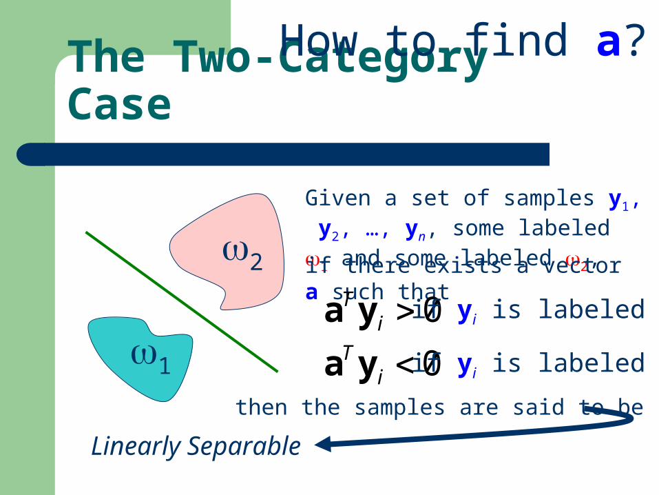
Linearly Separable
Given a set of samples y1, y2, …, yn, some labeled 1 and some labeled 2,
if there exists a vector a such that
0iT ya if yi is labeled 1
0iT ya if yi is labeled 2
then the samples are said to be
How to find a?
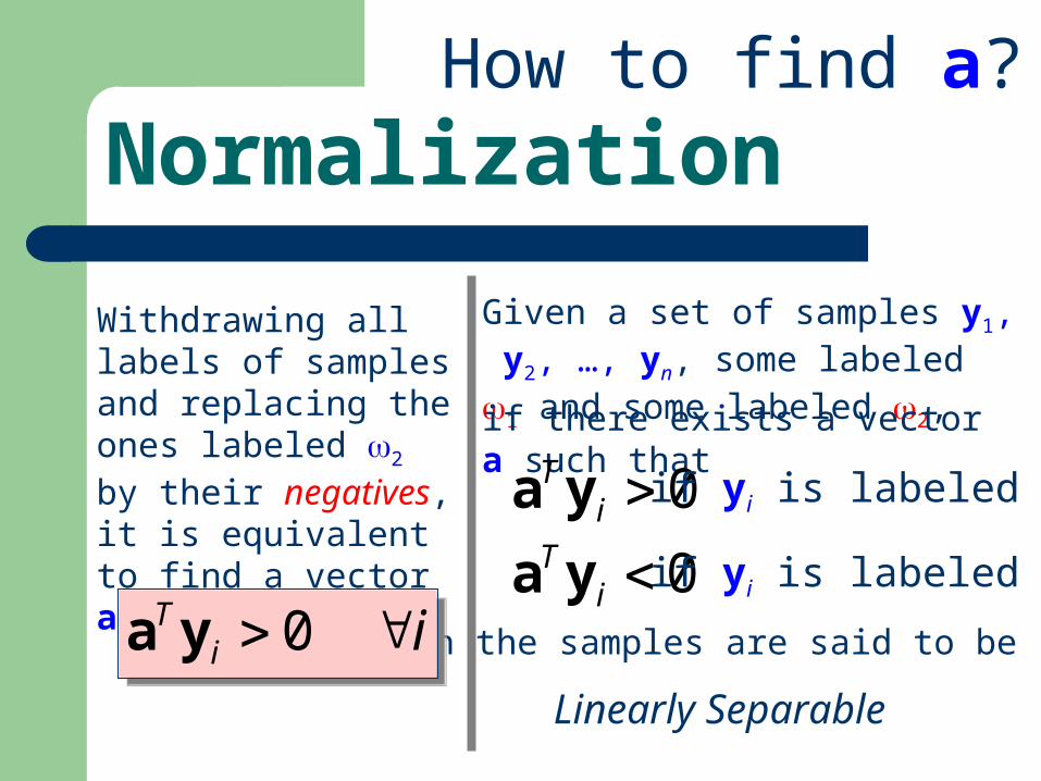
Normalization
Linearly Separable
Given a set of samples y1, y2, …, yn, some labeled 1 and some labeled 2,
if there exists a vector a such that
0iT ya if yi is labeled 1
0iT ya if yi is labeled 2
then the samples are said to be
Withdrawing all labels of samples and replacing the ones labeled 2 by their negatives, it is equivalent to find a vector a such that
iiT 0ya ii
T 0ya
How to find a?
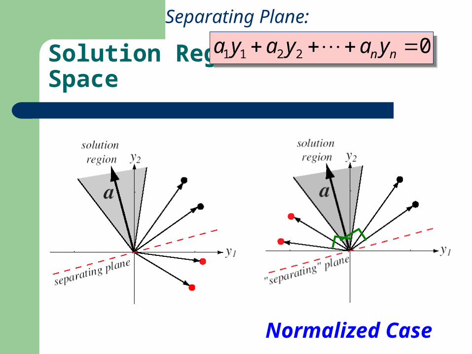
Solution Region in Feature Space
Normalized Case
Separating Plane:
02211 nn yayaya 02211 nn yayaya
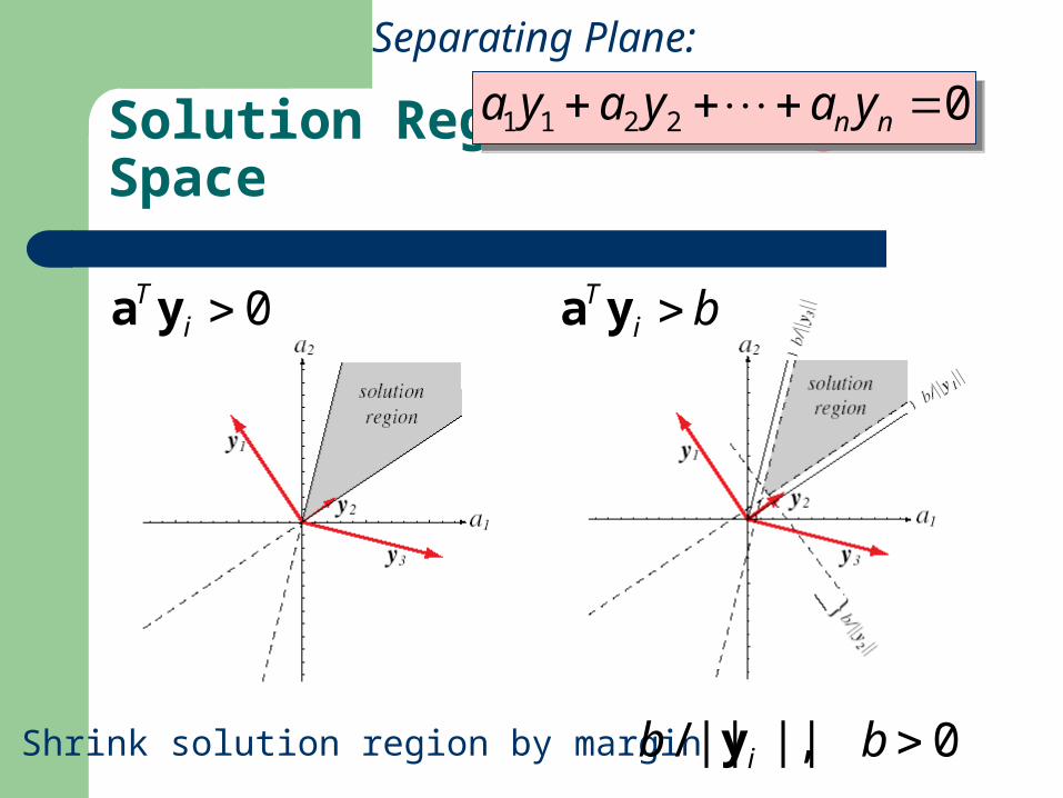
Solution Region in Weight Space
Separating Plane:
02211 nn yayaya 02211 nn yayaya
Shrink solution region by margin 0 , ||||/ bb iy
0iT ya bi
T ya

Linear Discriminant Functions
Learning

Criterion Function
To facilitate learning, we usually define a scalar criterion function.
It usually represents the penalty or cost of a solution.
Our goal is to minimize its value.
≡Function optimization.
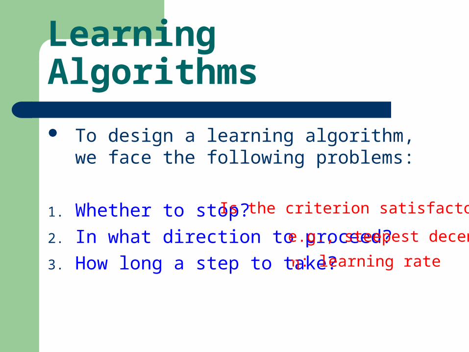
Learning Algorithms
To design a learning algorithm, we face the following problems:
1. Whether to stop?
2. In what direction to proceed?
3. How long a step to take?
Is the criterion satisfactory?
e.g., steepest decent
: learning rate

Criterion Functions:The Two-Category Case J(a)J(a)
# of misclassifiedpatterns
Is this criterion appropriate?
solution state
where to go?
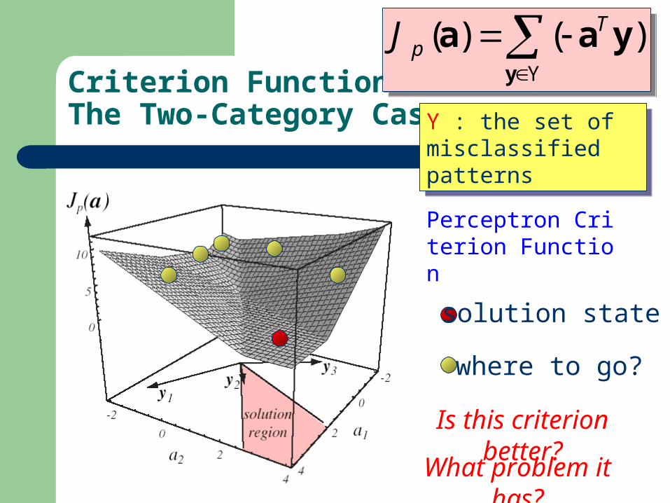
Criterion Functions:The Two-Category Case
Perceptron Criterion Function
solution state
where to go?
Is this criterion better?
)()( yaay
TpJ
Y
)()( yaay
TpJ
Y
Y : the set of misclassified patterns
Y : the set of misclassified patterns
What problem it has?
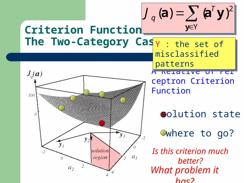
Criterion Functions:The Two-Category Case
A Relative of Perceptron Criterion Function
solution state
where to go?
Is this criterion much better?
2)()( yaay
TqJ
Y
2)()( yaay
TqJ
Y
Y : the set of misclassified patterns
Y : the set of misclassified patterns
What problem it has?
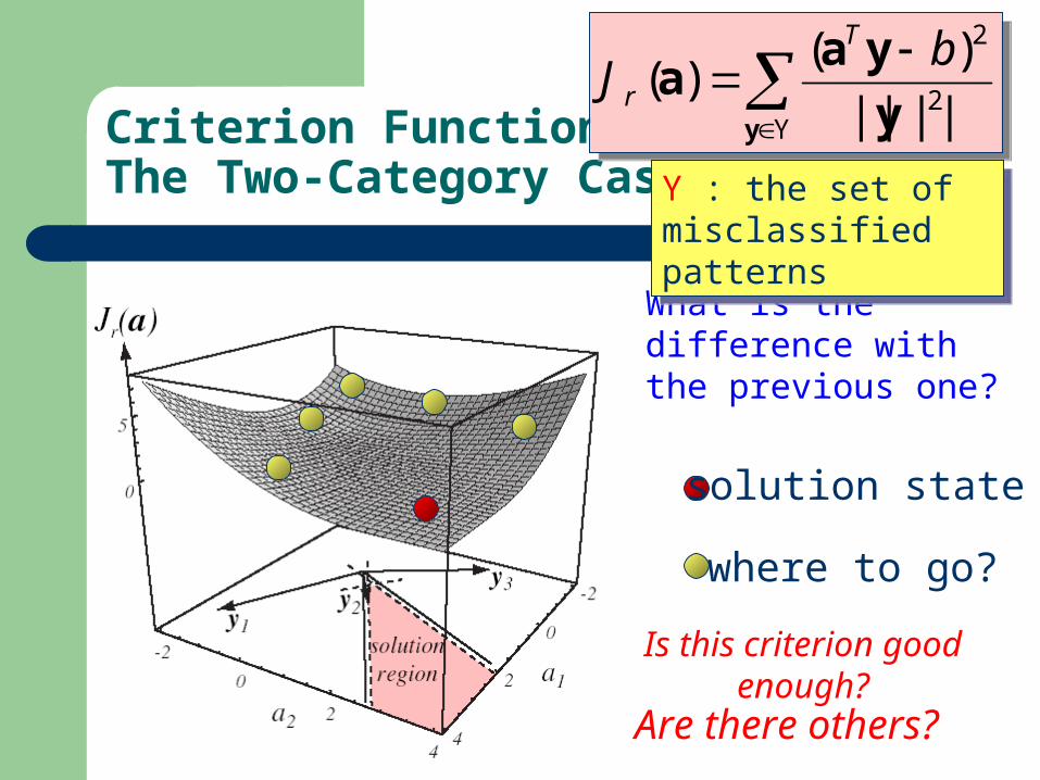
Criterion Functions:The Two-Category Case
What is the difference with the previous one?
solution state
where to go?
Is this criterion good enough?
Yy y
yaa
2
2
||||
)()(
bJ
T
r
Yy y
yaa
2
2
||||
)()(
bJ
T
r
Y : the set of misclassified patterns
Y : the set of misclassified patterns
Are there others?
Learning
Gradient Decent Algorithm
a1
a2J(a)
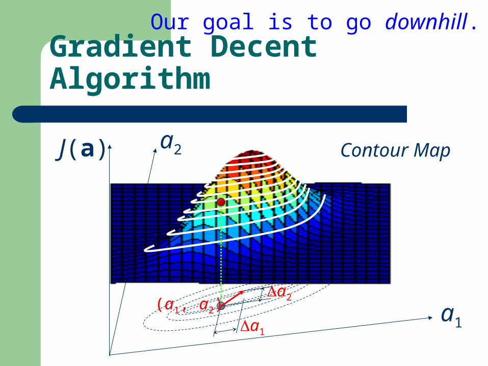
Gradient Decent Algorithm
Our goal is to go downhill.
Contour Map
(a1, a2)a1
a2
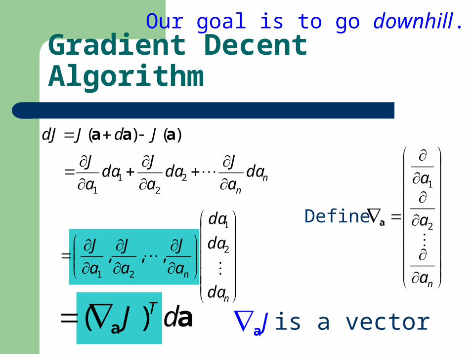
Gradient Decent Algorithm
Our goal is to go downhill.
)()( aaa JdJdJ
nn
daa
Jda
a
Jda
a
J
22
11
n
n
da
da
da
a
J
a
J
a
J
2
1
21
,,,
Define
na
a
a
2
1
a
aa dJ T)( aJ is a vector
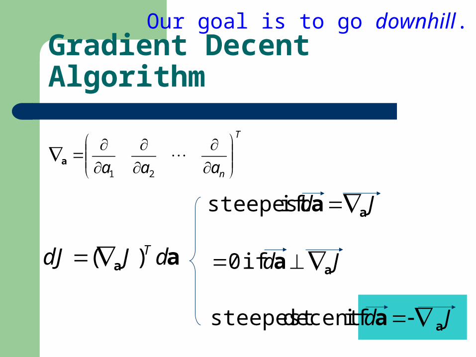
Gradient Decent Algorithm
Our goal is to go downhill.
T
naaa
21
a
aa dJdJ T)(
Jd aa ifsteepest
Jd aa if 0
Jd aa ifdecent steepest
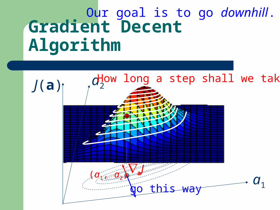
Gradient Decent Algorithm
Our goal is to go downhill.
a1
a2J(a)
(a1, a2)aJ
go this way
How long a step shall we take?
Gradient Decent Algorithm
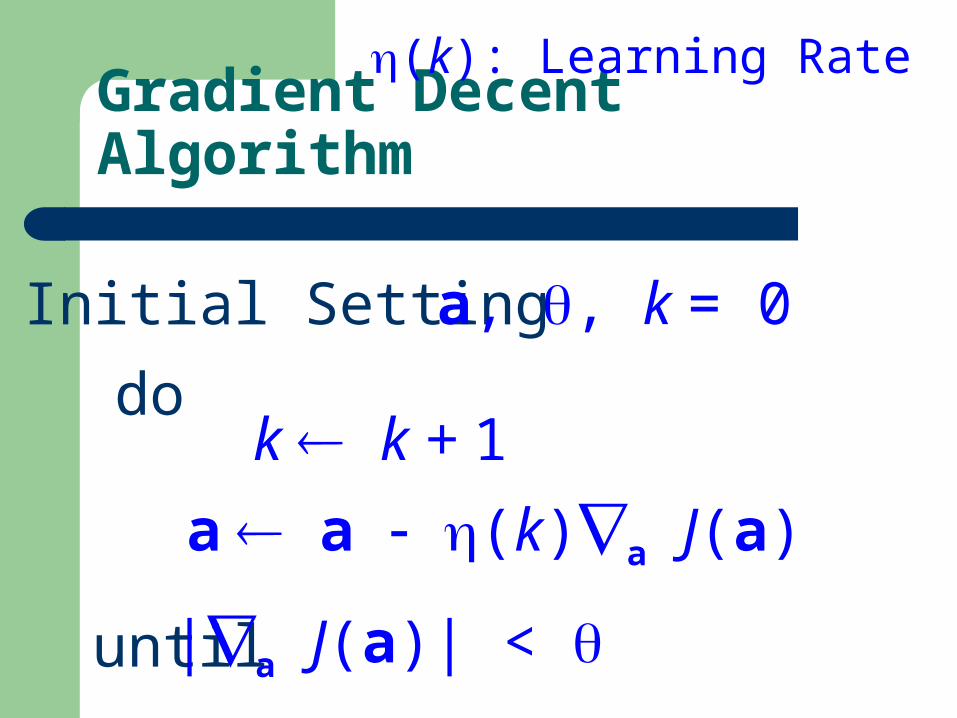
Initial Setting a, , k = 0
do k k + 1
a a (k)a J(a)
until |a J(a)| <
(k): Learning Rate
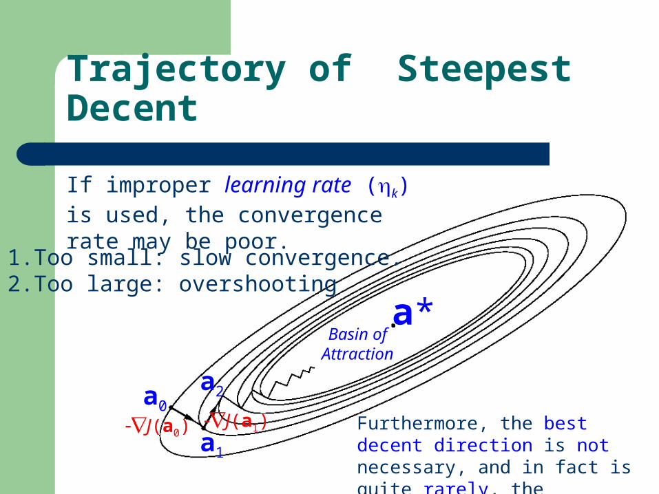
Trajectory of Steepest Decent
a*
a0
J(a0)a1
J(a1)
a2
If improper learning rate (k) is used, the convergence rate may be poor.
Basin of Attraction
1. Too small: slow convergence.2. Too large: overshooting
Furthermore, the best decent direction is not necessary, and in fact is quite rarely, the direction of steepest decent.
Learning Rate
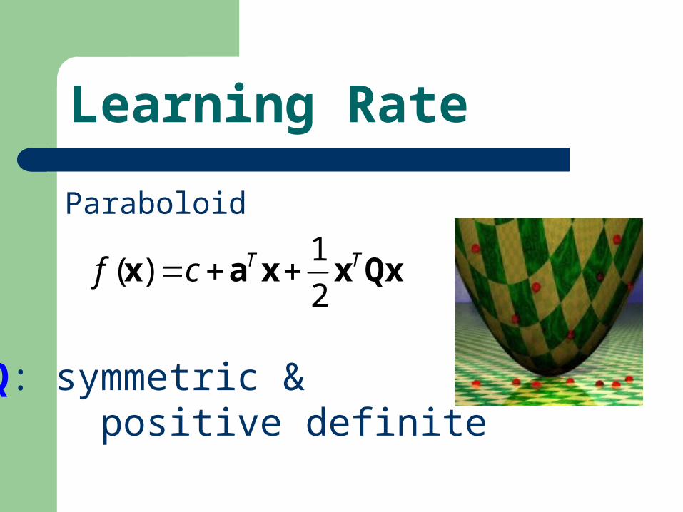
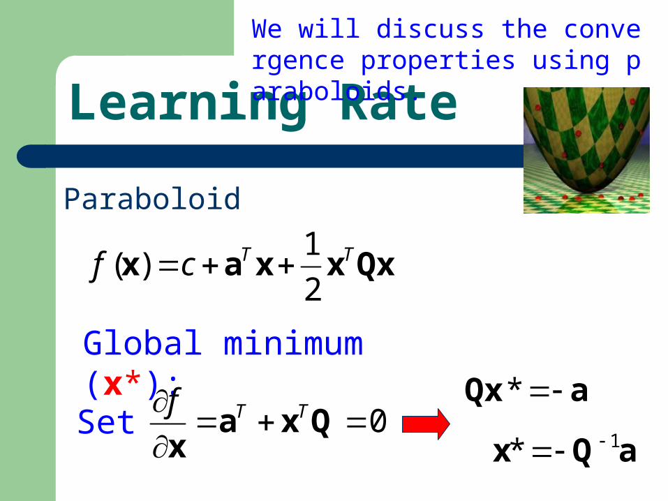
Paraboloid
Qxxxax TTcf2
1)(
Q: symmetric & positive definite
Learning Rate
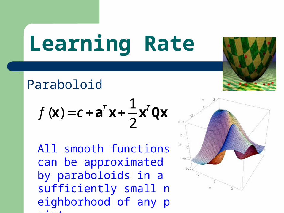
Paraboloid
Qxxxax TTcf2
1)(
All smooth functions can be approximated by paraboloids in a sufficiently small neighborhood of any point.
Learning Rate
Paraboloid
Qxxxax TTcf2
1)(
Global minimum (x*):
0
Qxax
TTfSet
aQx *
aQx 1*
We will discuss the convergence properties using paraboloids.
Learning Rate
Paraboloid
Qxxxax TTcf2
1)(
aQx * aQx * aQx 1* aQx 1*
Define *)()()( xxx ff
**2
1*
2
1QxxxaQxxxa TTTT
**2
1**
2
1* QxxxQxQxxxQx TTTTTT
*)(*)(2
1)( xxQxxx T *)(*)(
2
1)( xxQxxx T
Error
Learning Rate
Paraboloid
Qxxxax TTcf2
1)(
Define *)()()( xxx ff
*)(*)(2
1)( xxQxxx T *)(*)(
2
1)( xxQxxx T
*xxy
Error
Qyyy T
2
1)( Qyyy T
2
1)( We want to
minimize
0y *Clearly, 0*)( yand
Learning Rate
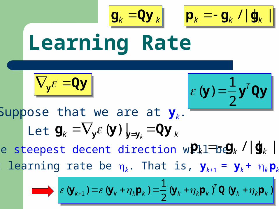
Qyyy T
2
1)( Qyyy T
2
1)( Qyy Qyy
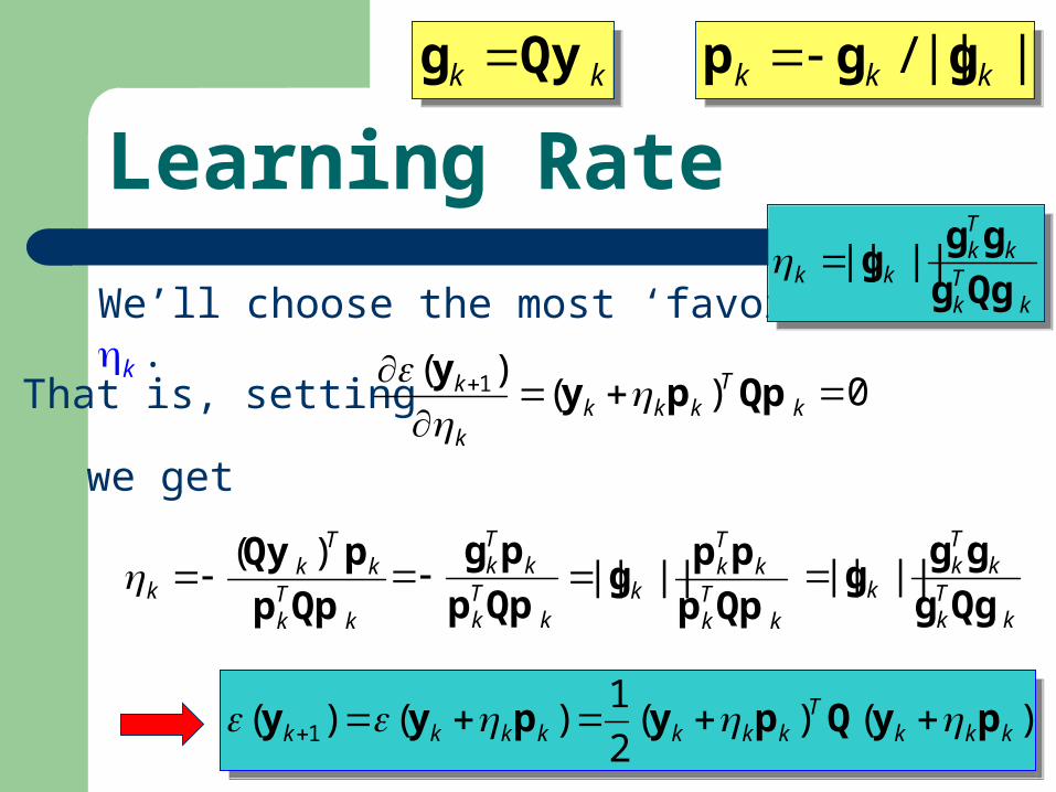
Suppose that we are at yk.
kk kQyyg yyy |)(Let
The steepest decent direction will be ||||/ kkk ggp Let learning rate be k. That is, yk+1 = yk + k pk.
)()(2
1)()( 1 kkk
Tkkkkkkk pyQpypyy
)()(2
1)()( 1 kkk
Tkkkkkkk pyQpypyy
||||/ kkk ggp ||||/ kkk ggp kk Qyg kk Qyg
Learning Rate
)()(2
1)()( 1 kkk
Tkkkkkkk pyQpypyy
)()(2
1)()( 1 kkk
Tkkkkkkk pyQpypyy
We’ll choose the most ‘favorable’ k .
That is, setting kT
kkkk
k Qppyy
)()( 1
0
we get
kTk
kT
kk Qpp
pQy )(
kTk
kTk
Qpp
pg
kTk
kTk
k Qpp
ppg ||||
kTk
kTk
k Qgg
ggg ||||
kTk
kTk
kk Qgg
ggg ||||
kTk
kTk
kk Qgg
ggg ||||
||||/ kkk ggp ||||/ kkk ggp kk Qyg kk Qyg

Learning Rate
kTk
kTk
kk Qgg
ggg ||||
kTk
kTk
kk Qgg
ggg ||||
kkkk pyy 1 kk
Tk
kTk
k gQgg
ggy
If Q = I,
*1 y0yyy kkk
||||/ kkk ggp ||||/ kkk ggp kk Qyg kk Qyg
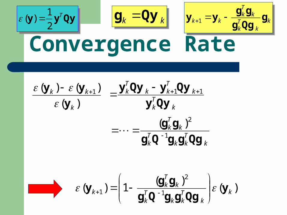
Convergence Rate
)(
)()( 1
k
kk
y
yy
Qyyy T
2
1)( Qyyy T
2
1)(
kk
Tk
kTk
kk gQgg
ggyy 1 k
kTk
kTk
kk gQgg
ggyy 1kk Qyg kk Qyg
kTk
kTkk
Tk
Qyy
QyyQyy 11
kTkk
Tk
kTk
QgggQg
gg1
2)(
)()(
1)(1
2
1 kk
Tkk
Tk
kTk
k yQgggQg
ggy

Convergence Rate
)()(
1)(1
2
1 kk
Tkk
Tk
kTk
k yQgggQg
ggy
The smaller the better
[Kantorovich Inequality] Let Q be a positive definite, symmetric, nn matrix. For any vector there holds
21
11
2
)(
4)(
n
nTT
T
QyyyQy
yy where 1 2 … n are eigenvalues of Q.
)()()(
41)(
2
1
12
1
11 k
n
nk
n
nk yyy
)()(
)(
41)(
2
1
12
1
11 k
n
nk
n
nk yyy
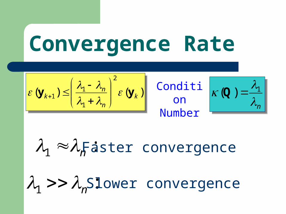
Convergence Rate
)()(2
1
11 k
n
nk yy
)()(
2
1
11 k
n
nk yy
Condition Number
n 1)( Q
n 1)( Q
:1 n
:1 n
Faster convergence
Slower convergence
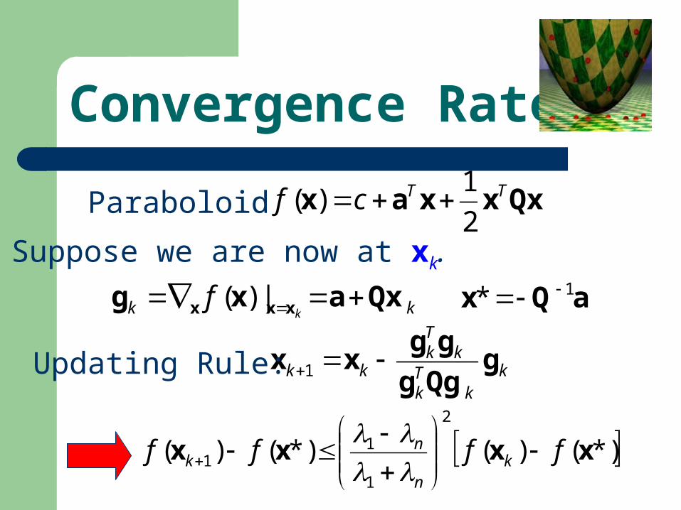
Convergence Rate
Paraboloid Qxxxax TTcf2
1)(
kk kf Qxaxg xxx |)(
Suppose we are now at xk.
kk
Tk
kTk
kk gQgg
ggxx 1Updating Rule:
aQx 1*
*)()(*)()(2
1
11 xxxx ffff k
n
nk

Trajectory of Steepest Decent
In this case, the condition number of Q is moderately large.
One then see that the best decent direction is not necessary, and in fact is quite rarely, the direction of steepest decent.
Learning
Newton’s Method

Global minimum of a Paraboloid
Paraboloid Qxxxax TTcf2
1)(
0|)( kkf Qxax xxx
We can find the global minimum of a paraboloid by setting its gradient to zero.
aQx 1*
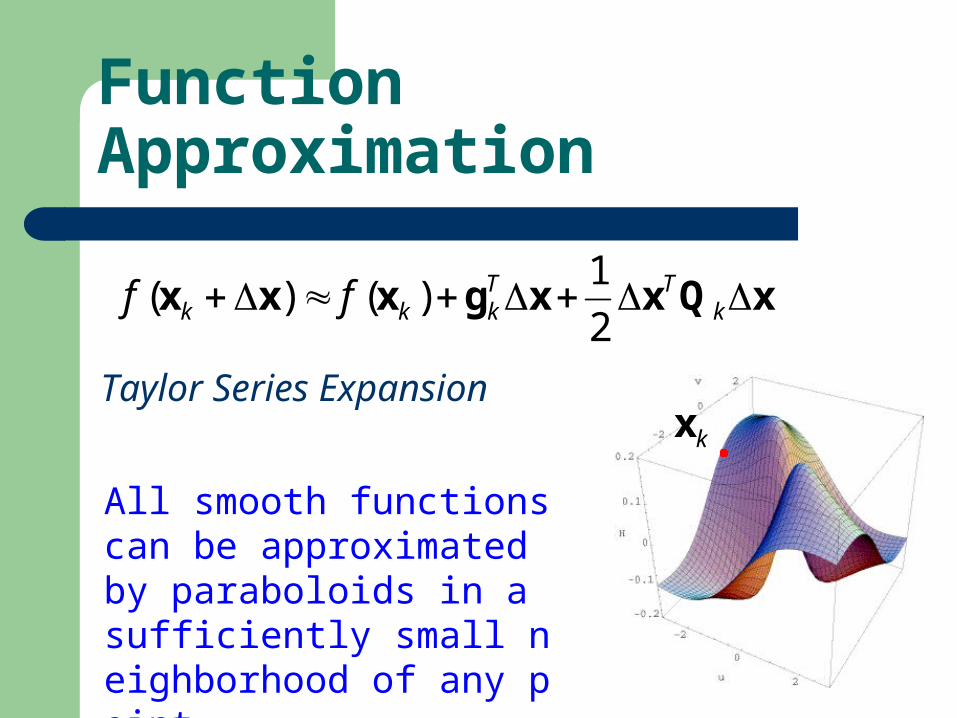
Function Approximation
All smooth functions can be approximated by paraboloids in a sufficiently small neighborhood of any point.
xQxxgxxx kTT
kkk ff2
1)()(
kxTaylor Series Expansion
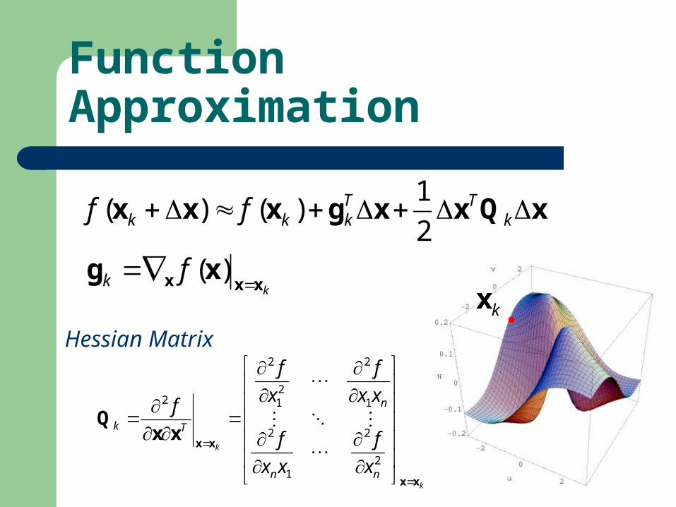
Function Approximation
xQxxgxxx kTT
kkk ff2
1)()(
kfk xxx xg
)(
kx
k
k
nn
n
Tk
x
f
xx
f
xx
f
x
f
f
xx
xxxx
Q
2
2
1
2
1
2
21
2
2
Hessian Matrix
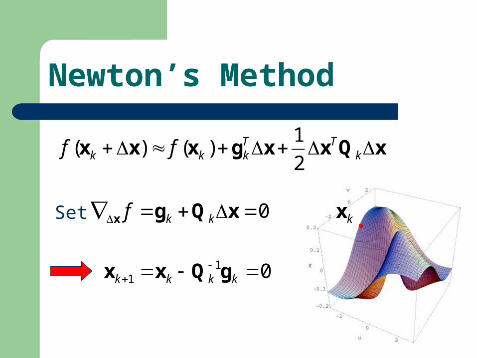
Newton’s Method
xQxxgxxx kTT
kkk ff2
1)()(
kx0 xQgx kkfSet
011 kkkk gQxx
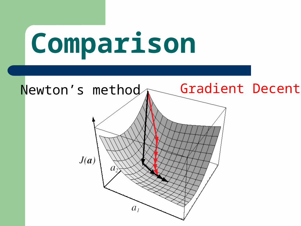
Comparison
Newton’s method Gradient Decent
Comparison Newton’s Method will usually give a greater improvement
per step than the simple gradient decent algorithm, even with optimal value of k.
However, Newton’s Method is not applicable if the Hessian matrix Q is singular.
Even when Q is nonsingular, compute Q is time consuming O(d3).
It often takes less time to set k to a constant (small than necessary) than it is to compute the optimum k at each step.