Leverage-Induced Fire Sales and Stock Market Crashes

September 5, 2017

PRELIMINARY, PLEASE DO NOT CITE

Abstract

This paper provides direct evidence of leverage-induced �re sales leading to a ma-jor stock market crash. Our analysis uses proprietary account-level trading data forbrokerage- and shadow-�nanced margin accounts during the Chinese stock market crashin the summer of 2015. We �nd that margin investors heavily sell their holdings whentheir account-level leverage edges toward their maximum leverage limits, controlling forstock-date and account �xed e�ects. Stocks that are disproportionately held by investorswho are close to receiving margin calls experience high selling pressure and signi�cantabnormal price declines that subsequently reverse over the next 40 trading days. Relativeto regulated brokerage accounts, unregulated and highly-leveraged shadow-�nanced mar-gin accounts contributed more to the market crash, despite the fact that these shadowaccounts held a much smaller fraction of market assets.

Leverage-Induced Fire Sales and Stock Market Crashes∗

Jiangze Bian Zhiguo He Kelly Shue Hao Zhou

September 5, 2017

PRELIMINARY, PLEASE DO NOT CITE

Abstract

This paper provides direct evidence of leverage-induced �re sales leading to a ma-jor stock market crash. Our analysis uses proprietary account-level trading data forbrokerage- and shadow-�nanced margin accounts during the Chinese stock market crashin the summer of 2015. We �nd that margin investors heavily sell their holdings whentheir account-level leverage edges toward their maximum leverage limits, controlling forstock-date and account �xed e�ects. Stocks that are disproportionately held by investorswho are close to receiving margin calls experience high selling pressure and signi�cantabnormal price declines that subsequently reverse over the next 40 trading days. Relativeto regulated brokerage accounts, unregulated and highly-leveraged shadow-�nanced mar-gin accounts contributed more to the market crash, despite the fact that these shadowaccounts held a much smaller fraction of market assets.

∗Jiangze Bian: University of International Business and Economics, jiangzebian@uibe.edu.cn; Zhiguo He:University of Chicago and NBER, zhiguo.he@chicagobooth.edu; Kelly Shue: Yale University and NBER,kelly.shue@yale.edu; Hao Zhou: PBC School of Finance, Tsinghua University, zhouh@pbcsf.tsinghua.edu.cn. Weare grateful to Will Cong, Zhi Da, Dong Lou, and Guangchuan Li for helpful discussions and insightful comments.Yiran Fan provided excellent research assistance.

1 Introduction

Excessive leverage and the subsequent leverage-induced �re sales are considered to be the underlying

causes of many past �nancial crises. A prominent example is the US stock market crash of 1929. At

the time, leverage for stock market margin trading was unregulated (margin requirements were not

imposed until the Securities and Exchange Act of 1934). Margin credit, i.e., debt that individual

investors borrow to purchase stocks, rose from around 12% of NYSE market value in 1917 to around

20% in 1929 (Schwert, 1989). In October 1929, investors began facing margin calls. As investors

quickly sold assets to deleverage their positions, the Dow Jones Industrial Average experienced a

record loss of 38.33 points, or 13%, in a single day, later known as �Black Monday� on October 28,

1929. The selling continued for a second day, as the Dow fell another 12% on October 29, 1929.1

Other signi�cant examples of deleveraging and market crashes include the US housing crisis which

led to the 2007/08 global �nancial crisis (see e.g., Mian et al. (2013)) and the Chinese stock market

crash in the summer of 2015. The latter market crash will be the focus of this paper.

As the worst economic disaster since the Great Depression, the 2007/08 global �nancial crisis

greatly revived the interest of academics and policy makers in understanding and measuring the

costs and bene�ts of �nancial leverage. In terms of academic research, the theory has arguably

advanced ahead of the empirics. For instance, Geanakoplos (2010) and Brunnermeier and Pedersen

(2009) carefully model a �downward leverage spiral,� in which tightened leverage constraints trigger

�re sales, which then depress asset prices, leading to even tighter leverage constraints. This general

equilibrium theory features a devastating positive feedback loop that is able to match various pieces

of anecdotal evidence, and is widely considered to be the leading explanation of the mechanism

behind the meltdown of the �nancial system during the 2007/08 crisis. Despite its widespread

acceptance, there is little direct empirical evidence of leverage-induced �re sales leading to stock

market crashes. Empirical tests of the theory are challenging because of the limited availability of

detailed account-level data on leverage and trading activity. This paper contributes to the literature

on leverage and �nancial crashes by providing direct evidence of leverage-induced �re sales.

1For a detailed description of the 1929 stock market crash, see Galbraith (2009).

1

We use unique account-level data in China that track hundreds of thousands of margin investors'

borrowing and trading activities. Our data covers the Chinese stock market crash of 2015, an

extraordinary period that is ideal for examining the asset pricing implications of leverage-induced

�re sales. The Chinese stock market experienced a dramatic increase in the �rst half of 2015, followed

by an unprecedented crash in the middle of 2015 which wiped out about 30% of the market's value

by the end of July 2015.2

Individual retail investors are the dominant players in the Chinese stock market and were the

main users of leveraged margin trading systems.3 Our data covers two types of margin accounts,

brokerage-�nanced and shadow-�nanced margin accounts, for the three-month span of May to July,

2015. Both margin trading systems grew rapidly in popularity in early 2015. The brokerage-�nanced

margin system, which allows retail investors to obtain credit from his/her brokerage �rm, is tightly

regulated by the China Securities Regulatory Commission (CSRC). For instance, investors must be

su�ciently wealthy and experienced to qualify for brokerage-�nancing. Further, the CSRC imposes

a market-wide maximum level of leverage�the Pingcang Line�beyond which the account is taken

over by the broker, triggering forced asset sales.4

In contrast, the shadow-�nanced margin system falls in a regulatory grey area. Shadow-�nancing

was not initially regulated of the CSRC, and lenders do not require borrowers to have a minimum

level of asset wealth or trading history to qualify for borrowing. There is no regulated Pingcang

Line for shadow-�nanced margin trades and maximum leverage limits are instead individually nego-

tiated between borrowers and shadow lenders. Not surprisingly, shadow accounts have signi�cantly

higher leverage than their brokerage counterparts.5 The shadow-�nanced margin accounts data is

particularly interesting because it is widely believed that excessive leverage taken by unregulated

shadow-�nanced margin accounts and the subsequent �re sales induced by the deleveraging process

2The Shanghai Composite Index started at around 3100 in January 2017, peaked at 5166 in mid-June, and thenwent dropped to 3663 at the end of July 2017.

3Trading volume from retail traders covers 85% of the total volume, according to Shanghai Stock ExchangeAnnual Statistics 2015, http://www.sse.com.cn/aboutus/publication/yearly/documents/c/tjnj_2015.pdf.

4The maximum leverage or Pingcang Line corresponds to the reciprocal of the maintenance margin in the US.5This con�rmed in our data: the equal-weighted average leverage (measured as assets/equity) is 6.62 for shadow

accounts and 1.43 for brokerage accounts.

2

were the main driving forces of the collapse the Chinese stock market.6 On June 12, 2015 the CSRC

released a set of draft rules that would tighten regulations on shadow-�nanced margin trading. A

month-long stock market crash started on the next trading day, wiping out almost 40% of the

market index. Using transaction-level data for shadow accounts, we examine the extent to which

shadow �nancing contributed to the market collapse.

We begin our empirical analysis by identifying the role of leverage constraints in a�ecting indi-

vidual investor trading behavior. For each account-date, we observe the account's leverage (de�ned

as the ratio of asset value to equity value) and �proximity to the Pingcang Line,� i.e., how close the

account's current leverage is to its Pingcang Line. Theories such as Brunnermeier and Pedersen

(2009) and Garleanu and Pedersen (2011) predict that investors will sell assets as the account's

leverage approaches its Pingcang Line. Costly forced sales occur if leverage exceeds the account's

Pingcang Line and the account is taken over by the lender. Forward-looking investors will sell as

the account's leverage approaches its Pingcang Line due to precautionary motives.7 We �nd strong

empirical support for these theories in the data: selling intensities of all stocks held in the account

increase as account-level leverage nears the Pingcang Line. The e�ect is non-linear, and increases

sharply when leverage is very close to the Pingcang Line.

Using variation in Pingcang Lines across shadow accounts, we further test how the level of lever-

age interacts with proximity to the Pingcang Line to a�ect individual selling behavior. Conditional

on the current level of proximity, leverage magni�es the sensitivity of each account's change in

proximity to any future changes in the value of assets held. This magni�cation channel may lead

investors with precautionary motives to delever if leverage is high, particularly if the account is

already close to hitting the Pingcang Line. Indeed, we �nd in the data that investors are much

more likely to sell assets if proximity and leverage are jointly high.

We also �nd evidence of strong interactions between leverage-induced selling, market movements,

6Common beliefs regarding the causes of the crash are discussed, for example, in a Financial Times article which isavailable at https://www.ft.com/content/6eadedf6-254d-11e5-bd83-71cb60e8f08c?mhq5j=e4. Another relevant read-ing in Chinese is in http://opinion.caixin.com/2016-06-21/100957000.html.

7In static models such as Brunnermeier and Pedersen (2009) and Geanakoplos (2010), �re-sales only occur whenthe account hits the leverage constraint (the Pingcang Line). However, in a dynamic setting such as Garleanu andPedersen (2011), forward looking investors start to sell before hitting the constraint.

3

and government regulations. We show that the relation between proximity and net selling is two to

three times stronger on days when the market is down rather than up. This result underscores how

leverage-induced �re sales in speci�c stocks feed into and are fed by broad market crashes. As more

margin accounts face leverage constraints, investors will seek to deleverage their holdings, which

will contribute to a market decline. As the market declines, leverage constraints tighten further,

causing investors to intensify their selling activities. We also �nd that government announcements

aimed at curbing excessive leverage may have intensi�ed leverage-induced selling in the short run,

triggering market-wide crashes. Further, government-mandated circuit breakers may have had the

unintended consequence of exacerbating �re sales crashes in other stocks that were not protected by

the circuit breakers. We �nd that investors seeking to deleverage signi�cantly intensify their selling

of unprotected stocks if other stocks in their portfolios cannot be sold due to stock-speci�c circuit

breakers.

In all the aforementioned analysis relating to account-level trading activity, we control for ac-

count �xed e�ects and stock-date �xed e�ects. Thus, the relation between proximity to the Pingcang

Line and selling intensity cannot be explained by the possibility that highly-leveraged investors tend

to be the types of investors that exhibit high selling intensity throughout the crisis period or that

stocks that are held by highly-leveraged accounts tend to be stocks that experience high selling

pressure for other reasons.

We then move on to show that stocks that are disproportionately held by margin accounts near

their Pingcang Lines experience high selling pressure. We classify accounts whose leverages are close

to (above a threshold of 0.6) to their Pingcang Lines as ��re sale accounts.� We then construct a

stock-date level measure of �re sale exposure, which measures the fraction of shares outstanding

held by �re sale accounts within our sample of margin accounts. We �nd that, controlling for stock

and date �xed e�ects, stocks with higher �re-sale exposure experience signi�cantly more net selling

volume from �re sale accounts.

Next, we explore the asset pricing implications of leverage-induced �re sales. Following Coval

and Sta�ord (2007), and using empirical re�nements developed in Edmans et al. (2012), we test

4

the prediction that �re sales should cause large price drops that revert in the long run. In our

setting, selling pressure from margin accounts close to their Pingcang Lines can cause �re sales

if there is insu�cient liquidity to absorb the selling pressure. These �re sales should cause stock

prices to drop in the short run and then to revert toward fundamental value in the long run when

liquidity returns to the market. We �nd strong support for this key prediction in our data. Stocks

with high �re sale exposure (i.e., stocks that are disproportionately held by margin accounts with

leverage close to their Pingcang Lines) signi�cantly underperform stocks with low �re sale exposure

in the short run, but these di�erences approach zero in the long run. Stocks in the top decile of

�re sale exposure underperform stocks in the bottom decile by approximately 5 percentage points

within 10 to 15 trading days, and the di�erence in performance reverts toward zero within 30 to 40

trading days. We �nd a similar U-shaped return response using regression analysis, which allows us

to better control for other factors that could in�uence returns, such as past returns, volatility, and

stock and date �xed e�ects.

Finally, our unique data sample allows us to perform the following forensic-style analysis: Given

that margin trading and leverage-induced �re sales indeed contributed to the Chinese stock market

crash of 2015, which margin trading system, brokerage or shadow, played a more important role?

Although practitioners, the media, and regulators have mainly pointed their �ngers at shadow-

�nanced margin accounts, the answer to this question is not obvious. First, according to many

estimates, total market assets held within the regulated brokerage-�nanced system greatly exceeded

that in the unregulated shadow-�nanced system. In our data, the multiple is about 4.5 at the peak of

the market boom. Second, and more importantly, brokerage-�nanced margin accounts have a lower

Pingcang Line that is uniformly imposed by the CSRC. Thus, even though brokerage accounts have

lower leverage on average, these account may also be closer to their Pingcang Lines. The tighter

Pingcang Line could turn more brokerage accounts into �re-sale accounts.

Section 2.2 investigates this question, and shows that the data strongly supports the view that

shadow-�nanced margin accounts contributed more to the market crash. We �nd that the leverage

of brokerage accounts remained low, even relative to their tighter Pingcang Lines. There were also

5

far fewer stock holdings in �re-sale accounts within the brokerage-�nanced system than within the

shadow-�nanced system. Further, a measure of �re sale exposure constructed from the shadow

accounts data sample o�ers much stronger explanatory power for price movements than a similar

�re sale exposure measure constructed from the brokerage accounts data sample.

Related Literature Our paper is related to the large literature on �re sales and their impact

on various asset markets including the stock market, housing market, derivatives market, and even

markets for real assets (e.g., aircrafts). In a seminal paper by Shleifer and Vishny (1992), the

authors argue that asset �re sales are possible when �nancial distress clusters at the industry level,

as the natural buyers of the asset are �nancially constrained as well. Pulvino (1998) directly tests

this theory by studying commercial aircraft transactions initiated by (capital) constrained versus

unconstrained airlines, and Campbell et al. (2011) documents �re-sales in local housing market due

to events such as foreclosures. In the context of �nancial markets, Coval and Sta�ord (2007) show

the existence of �re-sales by studying open-end mutual fund redemptions and the associated non-

information-driven sales; Mitchell et al. (2007) investigate the price reaction of convertible bonds

around hedge fund redemptions; and Ellul et al. (2011) show that downgrades of corporate bonds

may induce regulation-driven selling by insurance companies. Although �re-sales can be triggered

by many relevant economic forces, the original paper by Shleifer and Vishny (1992) focuses on the

force of deleveraging. In this regard, our paper di�ers from the previous empirical literature by

documenting a direct link between leverage, selling behavior, and �re sales, with the aid of account-

level leverage and trading data. Our paper also di�ers from previous empirical work on �nancial

markets which has mostly focused on examining �re sales in speci�c subsets of �nancial securities.

We show how leverage-induced �re-sales play a role in a broad stock market crash.

Our paper also contributes to the literature on the role of funding constraints, speci�cally margin

and leverage, in asset pricing. Theoretical contributions such as Kyle and Xiong (2001), Gromb and

Vayanos (2002), Danielsson et al. (2002), Brunnermeier and Pedersen (2009), and Garleanu and

6

Pedersen (2011), among others;8 help academics and policymakers understand these linkages in the

aftermath of the recent global �nancial crisis. There is also a large empirical literature that connects

various funding constraints to asset prices. Our paper follows a similar vein of investigating funding

constraints tied to the market making industry (e.g., Comerton-Forde et al. (2010) and Hameed

et al. (2010), among others).

Our paper is most closely related to the empirical literature which explores the asset pricing

implications of stock margins and related regulations. Margin requirements were �rst imposed

by Congress through the Securities and Exchange Act of 1934. Congress's rationale at the time

was that credit-�nanced speculation in the stock market may lead to excessive price volatility

through a �pyramiding-depyramiding� process. Indeed, Hardouvelis (1990) �nds that a tighter

margin requirement is associated with lower volatility in the US stock market. This is consistent

with an underlying mechanism in which tighter margin requirements discourage optimistic investors

from taking speculative positions (this mechanism also seems to �t unsophisticated retail investors

in the Chinese stock market). Hardouvelis and Theodossiou (2002) further show that the relation

between margin requirements and volatility only holds in bull and normal markets, but not in bear

markets. This �nding points to the potential bene�t of margin credit, in that it essentially relaxes

funding constraints. This trade-o� is cleanly tested in a recent paper by Tookes and Kahraman

(2016), which shows the causal impact of margin on stock liquidity using a regression discontinuity

design comparing stocks on either side of a margin eligibility regulatory threshold.9

Finally, our analysis and conclusions are complementary to a companion paper by Bian et al.

(2017), which uses the same dataset on margin traders in the Chinese stock market in 2015. Bian

et al. (2017) focuses on examining contagion among stocks held in the same leveraged margin

accounts and how the magnitude of the contagion can be ampli�ed through increased account

leverage. Bian et al. (2017) also show that this within-account contagion can be further transmitted

8Another important strand of literature explore the heterogeneous portfolio constraints in a general equilibriumasset pricing model and its macroeconomic implications, which features an �equity constraint;� for instance, Basakand Cuoco (1998); He and Krishnamurthy (2013); Brunnermeier and Sannikov (2014).

9As explained in Section 2.4, in China there also exists a list of stocks that are eligible for obtaining margincredit, but investors can purchase and hold non-eligible stocks in their margin accounts. As a result, both eligibleand non-eligible stocks are subject to leverage-induced �re-sales during the stock market crash.

7

across account networks, again ampli�ed by leverage. In contrast, this paper aims to provide direct

evidence of leverage-induced �re sales, which itself does not require contagion (although contagion

can of course feed and be fed by �re sales). This paper also di�ers from Bian et al. (2017), because

our analysis centers on the di�erence between the two types of margin accounts, regulated brokerage

accounts and unregulated shadow accounts. Our �ndings concerning the unique nature of shadow-

�nancing may help researchers and policymakers understand the role of regulation in the informal

�nance sector.

2 Institution Background

Our empirical analysis is based on the account-level margin trading data in Chinese stock market

covering the period from May 1, 2015 to July 31, 2015. We provide institutional background in this

section.

2.1 Margin Trading during the Chinese Stock Market Crash in 2015

The Chinese stock market experienced a dramatic increase in the �rst half of 2015, followed by an

unprecedented crash in the middle of 2015. The Shanghai Stock Exchange (SSE) composite index

started at around 3100 in January 2017, peaked at 5166 in mid-June, and then free-fell to 3663 at

the end of July 2017. It is widely believed that high levels of margin trading and the subsequent

�re sales induced by the de-leveraging process were the main driving forces of the market crash.10

There were two kinds of margin trading accounts active in the Chinese stock market during this

time period. One is brokerage-�nanced and the other is shadow-�nanced, as shown in Figure 1 which

depicts the structure and funding sources for the two margin trading systems.11 Both accounts were

nonexistent prior to 2010, but thrived after 2014 alongside the surge in the Chinese stock market,

10Common beliefs regarding the causes of the crash are discussed, for example, in a Financial Time article which isavailable at https://www.ft.com/content/6eadedf6-254d-11e5-bd83-71cb60e8f08c?mhq5j=e4. Another relevant read-ing in Chinese is in http://opinion.caixin.com/2016-06-21/100957000.html.

11In Chinese, they are called �Chang-Nei fund matching� and �Chang-Wai fund matching�, which, by literaltranslation, means �on-site� and �o�-site� �nancing. In a companion paper byBian et al. (2017) whose analysis isbased on the same data set as our paper, �shadow-�nanced� is called �peer-�nanced,� which emphasizes that margincredit can be supplied via either formal institutions like brokerage �rms or informal lending providers like wealthyindividuals.

8

which rose by 60% during the second half of 2014. In what follows, we describe these two types of

margin accounts in detail. Throughout the paper, whenever there is no risk of confusion, we often

use brokerage (shadow) accounts to refer to brokerage-�nanced (shadow-�nanced) margin accounts.

2.2 Brokerage-Financed Margin Accounts

Margin trading through brokerage �rms was �rst introduced to the Chinese stock market in 2010.

After its introduction, margin trading remained unpopular until around June 2014 when brokerage-

�nanced debt began to grow exponentially. The total debt held by brokerage-�nanced margin

accounts sat at 0.4 trillion Yuan in June 2014, but more than quintupled to around 2.2 trillion

Yuan within one year. This amounted to approximately 3-4% of the total market capitalization of

China's stock market in mid-June 2015, similar to the relative size of margin �nancing in the US

and other developed markets.

Brokerage-�nanced margin trades represented a highly pro�table business for brokerage �rms.

Brokers usually provide margin �nancing by issuing short-term bonds in China's intrebank market;

they can also borrow from the China Securities Finance Corporation (CSFC) at a rate slightly

higher than the interbank rate.12 Brokers then lent these funds to margin borrowers at an annual

rate of approximately 8-9%, who then combine their own equity funds to purchase stocks (the left

side of Figure 1).13 With risk-free rate around 4% at that time, this business o�ered brokers higher

pro�ts than commissions, which were only about 4 basis points (or 0.04%) of trading volumes during

this time period.

The regulatory body of the Chinese securities market, the China Securities Regulatory Com-

mission (CSRC), banned professional institutional investors from conducting margin trades through

brokers in China, implying that almost all brokerage-�nanced margin account holders were unsophis-

ticated retail investors. Due to concerns that a trading frenzy might destabilize the stock market,

the CSRC set very high quali�cation standards for investor to engage in brokerage-�nanced margin

12For a berief explanation on China Securities Finance Corporation (CSFC), seehttps://www.ft.com/content/c1666694-248b-11e5-9c4e-a775d2b173ca.

13For the rate at which the CSFC lent to security �rms, see http://www.csf.com.cn/publish/main/1022/1023/1028/index.html.For the rate at which security �rms lent to margin borrowers, see http://m.10jqka.com.cn/20170726/c599327374.shtml.

9

trading. A quali�ed investor needed to have a trading account with that broker for at least 18

months, with a total account value (cash and stockholdings combined) exceeding RMB 0.5 million.

CSRC sets the minimum initial margin to be 50% for brokerage-�nanced margin accounts, which

means that investors can borrow at most 50% of asset value when they open their brokerage accounts.

More importantly for our analysis, the CSRC also impose a minimum margin, which requires that

all brokerage-�nanced margin accounts maintain leverage below a universally applied maximum

limit. Brokerage-�nanced margin account could not have debt exceeding 1/1.3 of its current total

asset value (cash + stock holdings). Once the debt-to-assets ratio of a margin account increased

beyond 1/1.3, and if borrowers did not inject equity to reduce the account's debt-to-asset ratio the

next day, the account was subject to being taken over by brokerage �rms who then liquidated all

account holdings indiscriminately.

In China, practitioners call this maximum allowable leverage ratio, which equals Asset/Equity =

1.3/(1.3 − 1) = 4.33, the �Pingcang Line,� which means �forced settlement line� in Chinese. The

CSRC has been quite stringent in regulating brokerage-�nanced margin accounts, in the hopes that

that the relatively low maximum allowable leverage limit would prevent large-scale forced �re sales

that destabilize the market. This is consistent with the fact that, in our data, fewer than 1% of the

brokerage-�nanced margin accounts crossed the Pingcang Line and were taken over by brokers.

2.3 Shadow-Financed Margin Accounts

During the �rst half of 2015, many Chinese retail investors engaged in margin trading via the

shadow-�nancing system, in addition to, or instead of, the brokerage-�nancing system. Shadow-

�nanced (also called peer-�nanced) margin trading became popular among stock investors in 2014,

alongside the rapid growth of the Fintech industry in China. The shadow-�nancing system, similar

to many �nancial innovations in history, existed in a regulatory grey area. More speci�cally, shadow-

�nancing was not initially regulated of the CSRC, and the lenders did not require borrowers to have a

minimum level of asset wealth or trading history to qualify for borrowing. In turn, shadow-�nanced

borrowers were paying higher interest rates, usually 3-5 percentage points above their counterparts

10

in the brokerage-�nanced market (which is about 8-9%).

Shadow-�nancing usually operated through a web-based trading platform which provided various

service functions that facilitated trading and borrowing.14 The typical platform featured a �Mother-

Child� dual account system, with each mother account o�ering trading access to many (in most

cases, hundreds of) child accounts. The mother account, which is connected to a distinct trading

account registered in a brokerage �rm, belonged to the lender who was usually a professional lending

�rm. On the other hand, each child account was managed by individual borrowers, who were almost

all retail investors. Through this umbrella-style structure, a lender could lend funds to multiple retail

investors, while maintaining di�erent leverage limits for each borrower.

Similar to brokerage-�nanced margin accounts, shadow-�nanced margin accounts had maximum

allowable leverage limits�i.e., the Pingcang Line�beyond which the child account would be taken

over by the mother account (the lender), triggering �re sales. Due to the lack of supervision, unlike

brokerage-�nanced margin system, there were no regulation on the maximum allowable leverage for

each child account. Instead, the lender (the mother account) and the borrower (the child account)

directly negotiated the maximum allowable leverage limit for each account. As a result, shadow-

�nanced margin accounts had account-speci�c Pingcang Lines whereas brokerage-�nanced margin

accounts had a universal Pingcang Line of 4.33. In the data, the average initial debt-to-assets ratio

in shadow-�nanced margin accounts is much higher than that for brokerage accounts and shadow

accounts also have higher Pingcang Lines (the average Pingcang Line for shadow accounts is 15.3).

Whereas funding for brokerage accounts came from either the brokerage �rm's own borrowed

funds or from borrowing through the CSFC, funding for shadow-�nanced margin accounts came

from a broader set of sources that are directly, or indirectly, linked to the shadow banking system in

China. Besides the direct capital injection by �nancing companies who were running the shadow-

�nanced margin business, the three major funding sources were Wealth Management Products

(WMP) from commercial banks, Trust and Peer-to-Peer (P2P) informal lending, and borrowing

14HOMS, MECRT, and Royal Flush were the three leading electronic margin trading platforms in China during2015.

11

through pledged stock rights.15 The right hand side of Figure 1 lists these sources for shadow

margin traders to obtain credit; combining with their initial margins (equity) these investors then

traded on stocks through their child accounts.

Unregulated shadow-�nanced margin system was operated in the �shadow;� unlike the regulated

brokerage-�nanced peers, regurlators do not know the detailed breakdown of their funding sources,

let alone the total size of the shadow-�nancing market. According to the research report issued by

Huatai Securities, it is generally agreed that right before the stock market collapse in June 2015,

WMP peaked at around 600 billion Yuan and P2P informal lending peaked at about 200 billion

Yuan.16 For borrowing through pledged stock, it was illegal to use borrowed funds to purchase

stocks directly. However, during the �rst half of 2015, it was reported that some borrowers lent

these borrowed funds to professional lending �rms who then lent them out to shadow-�nanced

margin traders to purchase stocks. There is much less agreement on the quantity of pledged of

stock rights that �owed back into to the stock market through shadow-�nancing, and we gauge

250-500 billion Yuan to be a reasonable estimate.17 If we sum up these three sources, the estimated

total debt held by shadow-�nanced margin accounts was about 1.0-1.4 trillion Yuan at its peak,

consistent with the estimates provided by China Securities Daily on June 12, 2015.18

2.4 (Lack of) Regulation over Margin Accounts and the Stock Market Crash

The Chinese stock market stagnated for several years after the crisis of 2008 and began rapidly rising

around the middle of 2014. Recent research has argued that a major cause of the market boom was

the growth of margin trading,19 but with no corresponding growth in the real sector. Although the

government and professional traders warned that the stock market run-up may represent a bubble,

15A pledge of stock rights in China is an agreement in which the borrower pledges the stocks as a collateral toobtain credit, often from commercial banks.

16These estimates are given in Figure 1 of the report issued by Huatai Securities on July 5th, 2015, which isavailable at: https://wenku.baidu.com/view/565390bd43323968001c9234?pcf=2.

17According to the report by Huatai Securities, at early June 2015 the total borrowing through the pledged ofstock rights is about 2.5 trillion Yuan. Our estimate is based on the premise that about 10-20% of the borrowing areused to fund the leveraged stock investment via the shadow-�nanced margin system .

18http://news.xinhuanet.com/fortune/2015-06/12/c_127907477.htm.19Besides our papers, Huang et al. (2016) show that Chinese government's policies and the loose monetary policies

both support the growth of the stock market, and Bian et al. (2017) show that the outstanding debt of brokerage-�nanced margin trades closely tracks the Shanghai composite index level.

12

new investors continued to rush into the market and the index grew by 60% from the beginning to

the middle of 2015.

Besides regulating the maximum allowable leverage for brokerage-�nanced margin accounts, the

CSRC took other precautionary measures to prevent a leverage crisis in the stock market. The

CSRC mandated that only the most liquid stocks (usually blue-chips) were marginable, i.e., eligible

for investors to obtain initial margin �nancing. This regulation turned out to be futile because the

regulation only a�ected margin buying when the accounts were �rst opened. Investors in brokerage-

�nanced margin accounts were able to use cash from previous sales to buy other non-marginable

stocks. Broker �rms did not directly regulate this buying behavior and instead monitored whether

accounts had reached their Pingcang Lines; in fact, during the week of June 8-12 2015, 23% of stock

holdings in brokerage accounts are non-marginable stocks in our data. When the prices of stock

holdings in a leveraged brokerage account fell, the leverage rose, and investors engaged in either

preemptive sales to avoid approaching the Pingcang Line or forced sales because the account crossed

the Pingcang Line and was taken over by the lender. Regardless of the situation, investors sold both

marginable and non-marginable stocks indiscriminately, rendering the initial margin eligibility of

the stocks largely irrelevant when we study the role of leverage-induced �re sales in the stock market

crash.

More importantly, no such regulations existed in the shadow-�nancing market. Shadow-�nanced

margin investors could purchase any stock using margin as long as the total account leverage did not

exceed the negotiated account-speci�c Pingcang Line. No authoritative statistics are available for

the funding sources of these margin system, and this is why we place a grey �shadow� on the right

hand side of Figure 1. What regulators can see were several trading accounts (mother accounts)

that were formally registered in brokerage �rms with enormous trading volumes (aggregating all

trading orders from their child accounts).

While the shadow-�nancing market remained unregulated in the �rst half of 2015, many investors

and media outlets believed that the CSRC would release regulatory guidelines in the near future.

For instance, on May 22, 2015, newspapers reported that several securities �rms were engaging in

13

self-examinations of services provided to shadow-�nanced margin accounts, and that providers of

these �illegal� had received warnings from the CSRC as early as March 13, 2015.20 On June 12, 2015,

the CSRC released a set of draft rules that would strength the self-examinations of services provided

to shadow-�nanced margin accounts and explicitly ban new shadow-�nanced margin accounts.21

A month-long stock market crash started the next Monday on June 15, 2015, wiping out almost

40% of the market index. In response, the Chinese government began to aggressively purchase stocks

to support prices around July 9, and the market stabilized in mid-September. In this paper, we

show that leverage-induced selling pressure by margin investors, especially shadow-�nanced margin

investors, led to widespread �re sales that contributed to the crash in the interim period of June

and July 2015.

3 Data and Summary Statistics

We use a mixture of proprietary and public data from several sources. The �rst dataset contains

the complete equity holdings, cash balances, order submissions, and trade execution records of all

accounts from a leading brokerage �rm in China. The sample contains data on nearly �ve million

accounts, over 95% of which are retail accounts. Approximately 180,000 of these accounts are

eligible for brokerage-�nanced margin trading, hereafter referred to as �brokerage-�nanced margin

accounts� or �brokerage accounts.� The second dataset contains all trading and holding records

of more than 300,000 investor accounts from a large web-based peer-to-peer trading platform in

China. As explained, these �shadow-�nanced margin accounts� are borrowing from mother accounts,

and typically have substantially higher leverage than brokerage-�nanced margin accounts. After

applying �lters to focus on active accounts (with detalied provided in Appendix A), we retain a

sample of a little over 155,000 shadow-�nanced margin accounts.

A unique advantage of these two datasets is that we observe each margin account's end-of-day

leverage, de�ned as the account's total assets divided by the investor's own equity, where equity is

20See a review article in Chinese, available at http://opinion.caixin.com/2016-06-21/100957000.html.21See the Chinese version available at http://www.sac.net.cn/�gz/zlgz/201507/t20150713_124222.html.

14

the di�erence between total assets and debt.22 Together with these accounts' initial leverage and

end-of-day leverage, we can trace the daily evolution of leverage for each margin account.

Our data sample is representative of leveraged margin accounts in the Chinese stock market

as a whole. For brokerage-�nanced margin accounts, Shanghai Stock Exchange and Shenzhen

Stock Exchange publish daily the aggregate Yuan value of the debt �nancing provided to brokerage

accounts on their websites. On average, the debt �nancing in our brokerage-�nanced margin sample

accounts for 10% of the debt �nancing in the entire market. For shadow-�nanced margin accounts,

there are no o�cial statistics regarding its size as mentioned in Section 2.3. Several agencies have

o�ered rough estimates; among them, the estimates from Huatai Securities Co., who gauge that

the peak of debt funding going to shadow accounts is approximately 1-1.4 trillion Yuan, are widely

regarded as the most accurate ones. In our sample, the total debt in the shadow-�nanced margin

accounts peaked to around 56 billion Yuan in June 2015, which accounts for roughly 5% of the

estimated debt size of shadow accounts.

In terms of trading volume, the two datasets together account for roughly 10% - 15% of the total

trading volume reported by both the Shanghai Stock Exchange and Shenzhen Stock Exchange on

a typical day. Moreover, the cross-sectional correlation in trading volume between our two datasets

and the entire market is over 90%.23 These statistics all suggest that our data sample is fairly

representative of the aggregate market.

In addition to the two proprietary account-level datasets, we acquire daily closing prices, trading

volume, stock returns and other stock characteristics from the WIND database, which is widely

regarded as the leading vendor for Chinese market data.

22We observe daily leverage for all brokerage-�nanced margin accounts and about half of the shadow-�nancedmargin accounts. For the remaining shadow-�nanced margin accounts, we infer daily leverage from their initialdebt levels and subsequent cash �ows between these shadow �child� accounts and their associated lending �mother�accounts. See Appendix A for details.

23For each trading day, we estimate the cross-sectional correlation in trading volume between all stocks held inthe brokerage-�nanced accounts sample and each stock's total market volume. We then average across trading days.We repeat the analysis for the shadow-�nanced accounts sample.

15

3.1 Leverage

We de�ne leverage as

Levjt =Total AssetsjtEquityjt

(1)

for account j at the end of day t (this de�nition is similar to the one used in Ang et al, 2011 and

Bian et al, 2017) . Total Assetsjt is the total market value of assets held by account j at the end

of day t, including stock and cash holdings in Yuan value. Equityjt is equity value held by account

j at the end of day t, equal to total assets minus total debt. Under this de�nition, an account with

zero debt has leverage equal to 1.

The Pingcang Line is the maximum leverage beyond which the borrower will receive a margin

call, requiring her to either add more equity or liquidate her portfolio holdings to repay the debt.

If the borrower does not lower her leverage after receiving a margin call, her account may be taken

over by the lender. Although the lender is then expected to liquidate stock holdings to lower the

leverage, the lender may be unable to sell due to trading suspensions and price limits in the Chinese

stock market. In these cases, leverage can increase well above the Pingcang Line, while selling

pressure grows at a much slower pace. To reduce the in�uence of these outliers, we cap leverage at

100 in our analysis.

Figure 2 plots the end-of-day average leverage for the brokerage- and shadow-�nanced margin

account samples, together with the SSE composite index, which is widely used as the representative

market index in China. To compute the average, we weight each account's leverage by the equity in

each account. The average leverage is equal to total brokerage- or shadow-�nanced margin account

assets scaled by total brokerage- or shadow-�nanced margin account equity, respectively.

Figure 2 shows that, during the three month period from May to July 2015, average brokerage

leverage remains relatively �at, whereas average shadow leverage �uctuates dramatically. There is

a strong negative correlation between average shadow leverage and the SSE composite index. When

the SSE index increased from the beginning of May to the middle of June, average shadow leverage

declined. When the stock index began to plummet in the middle of June, average shadow leverage

16

grew and hit its peak around July 10th, when the index reached its lowest point. Overall, Figure

2 suggests that shadow-�nanced margin accounts may have been a driving force of the market

�uctuations in 2015, and that average shadow leverage displays a counter-cyclical trend.24

We can also contrast the equity-weighted average level of leverage (shown in the previous �gure)

with the asset-weighted average level of leverage in the market. Figure 3 shows that, relative to the

equity-weighted average, asset-weighted levels of leverage were much higher throughout our sample

period and sharply increased while the market crashed. This contrast illustrates the fact that highly

leveraged accounts with very little equity controlled a growing portion of market assets during the

market crash.

Figure 4 plots the dispersion within the account-level leverage distribution. We pool all brokerage-

and shadow-�nanced margin accounts, and plot the 20th, 50th, and 80th percentiles of the leverage

distribution within each day. We �nd that the 20th and 50th percentile lines remain relatively �at

throughout the sample period, whereas the 80th percentile line shows a similar trend to the aver-

age shadow leverage line in Figure 2, which runs countercyclical to the market index. Altogether,

these �gures suggests that trades from highly-leveraged shadow-�nanced margin accounts may help

explain stock market variation during our sample period.

Table 1 reports summary statistics for our data sample. We separately report statistics for

observations at the account-day, account-stock-day, and stock-day levels, where each day is a trading

day. In addition, we report statistics separately for the brokerage- and shadow-�nanced margin

account samples. Consistent with Figures 4 and 2, we �nd that shadow-�nanced margin accounts

are on average much more leveraged than brokerage-�nanced margin accounts. Average leverage

in shadow accounts are more then four times larger than leverage in brokerage accounts. Shadow

24There are two forces that drives the dynamics of leverage when asset prices �uctuate. The �rst is the passivevaluation e�ect, which drives leverage up when asset prices fall, by the de�nition of leverage (Asset/(Asset-Debt));this leads leverage to be counter-cyclical (e.g., He and Krishnamurthy (2013); Brunnermeier and Sannikov (2014)).The second is the active deleveraging e�ect, if investors respond to the negative fundamental shock by selling moreassets, which helps in generating a pro-cyclical leverage. Clearly, pro-cyclical leverage requires a stronger activedeleveraging e�ect, so much so that the resulting leverage goes down following falling asset prices (e.g., Fostel andGeanakoplos (2008); Geanakoplos (2010), and Adrian and Shin (2013)). He et al. (2017) discuss these two forces invarious asset pricing models in detail, and explain why the �rst valuation e�ect often dominates in general equilibriumand hence a counter-cyclical leverage ensues. In our sample, investors tend to keep their holdings in response to stockprice movement, which explains the counter-cyclical leverage pattern in Figure 2.

17

accounts also have Pingcang Lines that are, on average, more than three times larger than the

Pingcang Line of 4.3 that applies to all brokerage-�nanced margin accounts. Despite the fact that

shadow accounts tend to have higher maximum allowable levels of leverage, shadow accounts are also

closer to facing margin calls. On average, shadow accounts are more than four times closer to their

Pingcang Lines (and to receiving a margin call) than brokerage-�nanced margin accounts. Finally,

shadow accounts display substantially greater dispersion in leverage, with a standard deviation of

12.7 compared to a standard deviation of 0.5 for brokerage accounts.

In some analysis, we also use data from non-margin accounts as a benchmark for the trading

activity of unleveraged accounts. These accounts have zero debt and hence their leverage equal to

1. While these accounts are part of our brokerage dataset, these accounts are not included when

we refer to �brokerage accounts� which always refer to brokerage-�nanced margin accounts.

4 Results

In this section, we empirically test how account-level leverage relates to selling pressure, �re sales,

and asset prices. We begin by presenting analysis that pools the brokerage- and shadow-�nanced

margin account samples. In later analysis, we will show that the main e�ects appear to be driven

by the small pool of shadow-�nanced margin accounts that are highly leveraged.

4.1 Proximity to the Pingcang Line and Selling Intensity

We �rst show that account-level funding constraints, as measured by proximity to the Pingcang Line,

causes investors to sell assets to avoid margin calls. We construct the proximity to the Pingcang

Line as follows:

Pjt =Levjt − 1

Levj − 1(2)

where Pjt is the proximity of account j's leverage to its Pingcang Line at the end of day t. A higher

proximity implies the account is closer to receiving a margin call. Levjt is the leverage for account j

at the end of day t, and Levj is the Pingcang Line of account j. As explained in Section 3, although

18

Levj is the maximum allowable leverage for a margin account, Levjt may exceed Levj if investors

and lenders cannot sell their holdings due to trading suspensions. We sort Pjt into 10 equally spaced

bins, indexed by k and construct a dummy variable of Ijkt = 1 if Pjt ∈ [(k − 1)/10, k/10〉 where

k = 1, 2, ..., 10. We also create two additional bins: bin 0 for unleveraged accounts (Pjt = 0 is

classi�ed in bin 0 rather than bin1), and bin 11 for accounts with Pjt ≥ 1, which occurs if Levjt

exceeds Levj .

We then examine how proximity to the Pingcang Line a�ects investor selling. We estimate the

following regression

δjit =

11∑k=1

λkIjk,t−1 + νit + αj + εjit (3)

where δjit is account j's net selling volume of stock i on day t, normalized by account j's shares

held of stock i at the beginning of day t. Because we are interested in selling behavior, the sample

is restricted to stocks held by account j at the start of day t. Net buying results in negative

values for δjit, which we limit fro below at -1.2. We regress net selling δjit on dummy variables for

each bin representing proximity to the Pingcang Line. The omitted category is bin 0, representing

unleveraged brokerage accounts. The main coe�cients of interest are the selling intensities λk,

which measure the di�erence in selling intensity within each bin relative to the omitted category of

unleveraged accounts. If closeness to the Pingcang Line causes net selling, we expect that the selling

intensity λk will increase with k. To isolate the e�ect of each margin account's speci�c time-varying

funding constraints on selling intensity, we also control for stock-date �xed e�ects νit and account

�xed e�ects αj . These �xed e�ects control for the possibility that all accounts in our sample may

be more likely to sell a stock on a particular day or that some accounts are more likely to sell than

others on average during our sample period.

Figure 5 shows the selling intensity λk for each bin representing proximity to the Pingcang Line.

The regression analogue for the �gure is presented in Column 1 of Table 2. We �nd that λk increases

with k, consistent with our conjecture that closeness to margin limits induces investors to sell their

holdings. Relative to unleveraged accounts, accounts in bin 10 (where leverage is within 10% of the

19

Pingcang Line) increase net selling by 0.18, equivalent to 60% of a standard deviation in the level

of net selling activity across accounts.

We also �nd that λk is close to zero for accounts that are far away from their Pingcang Lines, and

that λk increases sharply when Pjt approaches 0.6. Therefore, we de�ne accounts with a proximity

to the Pingcang Line greater than 0.6 as ��re sale accounts.� These accounts are signi�cantly more

likely to face funding constraints and to contribute to �re sales of assets. In later tests, we also

show that our results are not sensitive to the exact 0.6 cuto�.

4.2 Leverage Ampli�cation and Asymmetry in Market Condition

Next, we examine how tightened leverage constraints (as proxied by proximity to the Pingcang

Line) interacts with each account's level of leverage. An increase in leverage has the direct e�ect of

moving each account closer to its Pingcang Line, thereby increasing its proximity. Controlling for

the accounts current level of proximity, leverage should still matter, because leverage ampli�es the

sensitivity of each account's change in proximity to any future �uctuations in the market value of

the stocks held by the account. This ampli�cation channel may lead investors with precautionary

motives to delever more facing higher leverage, particularly if the account is already close to hitting

the Pingcang Line.

We test this mechanism by analyzing how selling intensity is a�ected by proximity, leverage, and

the interaction between leverage and an indicator for whether the account is close to its Pingcang

Line (a �re sale account). We focus this analysis on shadow-�nanced margin accounts, because

Pingcang Lines vary across shadow-�nanced margin accounts, allowing us to separately identify

the e�ects of proximity, leverage, and potential interactions. Note, we cannot do this analysis for

the brokerage sample, because all accounts have the same Pingcang Line, so there is a one-to-one

mapping between leverage and proximity.

In Table 3, we regress net selling on proximity bins as de�ned before, �ve bins in leverage,

interactions between the leverage bins and an indicator for �re sale accounts, as well as stock-date

�xed e�ects and account �xed e�ects. We �nd that proximity continues to predict higher selling

20

intensity, after controlling for leverage. Moreover, the interaction between the largest leverage bins

and the indicator for �re sale accounts is signi�cantly positive. This implies that, controlling for

proximity, investors are more likely to sell assets if proximity and leverage are jointly high. We

also �nd that the relation between net selling and leverage is non-linear. While very high leverage

predicts increased net selling, the relation between leverage and net selling is reversed conditional

on leverage being among the lower bins. This empirical pattern is consistent with the view that

investors choose to take on more leverage when they are feeling more bullish and/or speculative

and therefore are more likely to buy rather than sell assets, holding leverage constraints (proximity)

constant. However, as leverage constraints begin to bind, investors become more likely to sell assets

if the level of leverage is also high.

Another important prediction for leverage downward spiral (e.g., Brunnermeier and Pedersen

(2009)) is the asymmetry between market downturn versus upturn, a phenomenon widely docu-

mented by Hameed et al. (2010), Tookes and Kahraman (2016), and Bian et al. (2017) in various

related contexts. Figure 6 and Table 4 show how proximity to the Pingcang Line a�ects selling

intensity, conditional on whether the market return is positive or negative on day t; and we �nd ev-

idence of strong interactions between leverage-induced selling and market movements. Importantly,

even if the market does well, precautionary motive suggests that margin investors with leverage

being closer to the Pingcang Line should exhibit higher selling intensity. What is more, conditional

on a given proximity to the Pingcang Line at the start of day t, leverage constraints will tighten

further on average if the market return over day t is negative. Thus, we expect that the relation

between proximity and selling intensity will be stronger if the market return on day t is negative.

Consistent with these predictions, we �nd that higher proximity leads to higher selling intensity

even when market returns are positive. We also �nd that the relation between proximity and net

selling is two to three times stronger on days when the market is down. These results underscore

how leverage-induced �re sales in speci�c stocks feed into and are fed by broad market crashes.

As more margin accounts face leverage constraints, investors will seek to deleverage their holdings,

which will contribute to a market decline. As the market declines, leverage constraints tighten

21

further, causing investors to intensify their selling activities, conditional on each level of proximity.

4.3 Fire Sale Exposure and Selling Pressure

Selling pressure occurs when more investors wish to sell a stock than can quickly be absorbed

by investors on the other side. Selling pressure can lead to �re sales in which stocks trade below

fundamental value. We hypothesize that stocks that are disproportionately held by leveraged margin

accounts that are close to their Pingcang Lines are more exposed to �re sale risk. We expect that

these stocks are more likely to experience selling pressure from highly-leveraged margin accounts,

i.e., accounts with Djt > 0.6 that we classify as �re sale accounts. To test this hypothesis, we de�ne

stock i's �re sale exposure (FSE) on day t as:

FSEit =total shares of stock i held in �re sale accounts at the beginning of day t

outstanding shares of stock i on day t. (4)

In the numerator, we only count the number of shares held by margin accounts that are classi�ed as

�re sale accounts as of the start of day t. Table 1 presents summary statistics of our FSE measure.

As expected, FSE calculated using the shadow-�nanced margin account sample is double that

calculated using the brokerage-�nanced margin account sample, consistent with shadow accounts

being closer to their Pingcang Lines on average. In this section, we again focus on the pooled sample

of brokerage- and shadow-�nanced margin accounts, and reserve subsample analysis for Section 4.5.

We estimate the following regression to examine the e�ect of FSE on stock-level selling pressure:

δit = β · FSEit + controlsit + si + τt + εit. (5)

δit measures stock-level selling pressure from �re sale accounts. We calculated δit as the total net

selling volume of stock i on day t from all �re sale accounts that hold stock i at the start of day

t, scaled by the number of outstanding shares of stock i at the beginning of day t. Controlsit is a

vector of control variables including the stock's volatility and turnover in the past 60 days, market

capitalization measured in t− 3, and 10 variables for the stock's daily returns in the past 10 days.

22

We also control the stock �xed e�ects si and date �xed e�ects τt.

Table 5 presents the regression results corresponding Equation 5. Across all speci�cations, we

�nd that �re sale exposure signi�cantly increases stock-level selling pressure. The estimates in

Column 4 of Panel A imply that a one standard deviation increase in FSE increases the selling

pressure of each stock by 40% of a standard deviation.

We also �nd that �re sale exposure (the fraction of shares of each stock held by �re sale accounts)

can explain a substantial amount of the variation in our measure of selling pressure. We �nd that

a regression of selling pressure on FSE alone, with no other control variables, yields an r-squared of

14.4%. This r-squared is large relative to the r-squared of 18.7% obtained from a more saturated

regression in which we also control for stock and date �xed e�ects, past returns, and a large set

of other time-varying stock characteristics. Thus, FSE can explain a substantial percentage of the

variation in selling pressure from highly-leveraged accounts, and controlling for additional stock

characteristics only marginally adds to the explanatory power of the regression.

4.4 Fire Sale Exposure and Stock Prices

In this section, we show how �re sale exposure a�ects stock prices. Selling pressure from margin

accounts close to their Pingcang Lines can cause stock-level �re sales if there is insu�cient liquidity

in the market to absorb the selling pressure. These �re sales should cause stock prices to drop below

fundamental value in the short run. In the long run, prices should revert to fundamental value if

liquidity returns to the market. Thus, we expect stocks with high FSE to under-perform stocks

with low FSE over the short-run and to revert to similar levels in the long-run. We present two

empirical strategies to test this conjecture.

4.4.1 Double Sorts

We begin by exploring abnormal returns to a double-sorted long-short portfolio. On each trading

day t, we sort all stocks held by �re sale accounts into four quartiles according to their return

over the period [t − 10, t − 1]. Within each quartile, we then sort stocks into 10 bins according to

23

their FSE at the start of each day t. For each quartile of previous period returns, we construct a

long-short strategy that longs the bin with the highest FSE and shorts the bin with the lowest FSE.

In Figure 7, we plot the cumulative returns for this long-short strategy, averaged across all

days t. For all four quartiles of past 10-day returns, we �nd a distinct U-shape for the cumulative

abnormal returns of the long-short portfolio. The �gures show that, controlling for past returns,

stocks in the top decile of FSE underperform stocks in the bottom decile of FSE by approximately

5 percentage points within 10 to 15 trading days after the date in which FSE is measured. The

di�erence in performance reverts toward zero with 30 to 40 trading days.

4.4.2 Regression Analysis

To better account for other factors that could lead to di�erential return patterns for high and low

FSE stocks, we turn to regression analysis. We estimate the following regression:

CARi,t+h = γh · FSEit + controlsit + si + τt + εit (6)

where CARi,t+h is the cumulative abnormal return for stock i from day t to t+h. Here, the abnormal

return is estimated relative to the CAPM, with beta for each stock calculated using year 2014 data.

We control for stock and day �xed e�ects. We also control for each stock's return volatility and

turnover over the past 60 trading days, market value in t−3, and cumulative and daily returns over

the past 10 trading days. If FSE has a negative short-run e�ect on stock returns that reverts in the

long run, we expect γh < 0 for small h and γh = 0 for large h.

Table 6 presents regression results for return windows h = 1, 3, 5, 10, 20, and 40 trading days.

We �nd that FSE measured at the start of trading day t leads to signi�cant price declines in the �rst

10 trading days after day t, but the price declines revert toward zero by approximately 40 trading

days after day t.

24

4.5 Brokerage- vs. Shadow-Financed Margin Accounts

As explained in Section 2, there were two types of leveraged margin accounts active during the

Chinese stock market crash of 2015. In short, brokerage-�nanced margin accounts were managed

by certi�ed brokerage �rms, and were heavily regulated with lower maximum allowable leverage

levels (lower Pingcang Lines) and lower average levels of leverage relative to their Pingcang Lines.

Meanwhile, shadow-�nanced margin accounts conducted trading and borrowing on web-based plat-

forms, were free from regulation, and had much higher leverage. Since the onset of the stock market

crash in early June 2015, shadow-�nanced margin accounts have been widely accused as the driv-

ing force behind the market collapse. However, this accusation has largely been untested using

concrete evidence. With the aid of our detailed account-level data, we investigate this question in

this subsection. We believe our �ndings can shed light on the potential interactions between the

unregulated and regulated sectors.

4.5.1 Selling Intensities for Brokerage and Shadow accounts

In Section 4.1, we showed that accounts tend to sell more of their stock holdings when they are

closer to their account-speci�c Pingcang Lines, and we classi�ed �re-sale accounts as those with

proximity to the Pingcang Line above the cuto� of 0.6 (i.e., Pjt > 0.6 as in Equation 2). We now

repeat the exercise separately for the brokerage- and shadow-�nance margin account samples. The

estimated selling intensities (λk's) for each account type are plotted in Figure 8 and the correspond-

ing regression coe�cients are presented in Table 2 Column 2 and 3. We �nd that the estimated

selling intensities increase with the proximity to the Pingcang Line for both samples, consistent

with the leverage-induced �re-sales mechanism.

There are several features in Figure 8 worth discussing. First, conditional on a bin for proximity

to the Pingcang Line, selling intensities are much larger for shadow accounts. In fact, for Pjt in the

range between 0.5 and 1, the selling intensity in shadow accounts is about twice as large as that

of brokerage accounts. This result is intuitive because, conditional on a proximity to the Pingcang

Line bin, shadow accounts have higher leverage than brokerage accounts (the former has higher

25

Pingcang Lines than the latter). As shown earlier in Table 3, when we compare the net selling of

the same stock on the same day, held by two accounts with the same proximity to the Pingcang

Line, the higher leverage of the shadow accounts will amplify any negative fundamental shock (of

stock price), leading to more precautionary selling behavior by shadow account holders.

Second, once either account type crosses over the Pingcang Line and is taken over by the lender

(the last bin with Pjt > 1), the selling intensity of brokerage accounts rises dramatically, and is even

slightly higher than that of shadow accounts. At this point, the lender starts to aggressively sell all

assets, and di�erences in borrowers' precautionary motives across brokerage and shadow account

types no longer matter.25

We also investigate how the selling intensities of brokerage and shadow accounts di�er in their

responses to the regulatory shocks that occurred before the onset of market crash. As mentioned

toward the end of Section 2.3, two regulatory tightening announcements were made which had

to potential to trigger spikes in the selling intensities of leveraged accounts: the May 22 event in

which some brokerage �rms were required to self-examine their provision of services toward shadow-

�nanced margin accounts, and the June 12 event in which the CSRC released a set of draft rules

that explicitly banned shadow accounts.

For both events, we estimate λk's for the �ve trading days before and after the regulatory

announcements, which were released after-hours on Fridays. The results are plotted in Figure 7, and

detailed regression results are presented in Table 7. We �nd that the two regulatory announcements

led to small and inconsistent changes in the selling intensities for brokerage accounts (note that

very few brokerage occupied the far right bins, so the estimated selling intensities for those far right

bins are insigni�cantly di�erent from zero). In contrast, news of regulatory tightening signi�cantly

increased the selling intensities of shadow accounts within each bin for proximity to the Pingcang

Line. The June 12 announcement, in particular, led to more than a tripling of selling intensities for

25It is interesting to observe that shadow accounts, after being taken over by lenders, exhibit less aggressive sellingbehaviors than similarly defaulted brokerage accounts. Although our data does not allow us to investigate this issuefully, one plausible explanation is that some lenders of shadow accounts may be wealthy individual investors whoexercise discretionary selling once they gain control of defaulted shadow accounts. In contrast, lenders of brokerageaccounts are brokerage �rms who have more stringent risk management systems.

26

shadow accounts with proximity greater than 0.6. This evidence is consistent with the widely-held

view that news of potential future regulatory tightening triggered �re sales by shadow accounts.

4.5.2 Circuit Breakers and Selling Intensity

During our sample period of May to July 2015, each individual stock was allowed to move a daily

maximum of 10 percent from the previous closing level in either direction, before triggering a circuit

breaker which would halt all trading for the stock for the rest of the day. These circuit breakers

were introduced with the goal of suppressing excessive trading and controlling market volatility.

However, the circuit breakers may have had the unintended consequence of exacerbating �re sales

crashes in other stocks. As we've shown in Table 2, margin investors are signi�cantly more likely

to sell assets when their account-level leverage nears their Pingcang Line limit. We hypothesize

that an investor seeking to deleverage may further intensify the selling of a particular stock if other

stocks in her portfolio cannot be sold due to stock-speci�c circuit breakers.

We �nd strong support for this hypothesis in the data. For each account-day, we de�ne �price

limit� as the fractional value of account j's assets as of the start of day t that consist of stocks

that hit price limits at some later point on day t. Price limit measures the extent to which margin

investors are constrained in their ability to sell a subset of their holdings due to circuit breakers.

We then regress net selling at the account-stock-day level on the set of proximity bins de�ned

earlier, price limits, and the interaction between price limits and the proximity bins. We restrict

the regression sample to stocks that do not face trading restrictions on day t. The results for

the full sample are reported in Table 8 Column 1. As expected, we �nd that accounts with higher

proximity are signi�cantly more likely to sell. Moreover, the interaction between proximity and price

limit is signi�cant and positive for all proximity bins, and increasing in magnitude with proximity.

This is consistent with investors being more likely to sell any particular stock in their portfolio if

other holdings cannot be sold due to circuit breakers, with the e�ect being larger for investors with

stronger deleveraging motives (i.e., those with higher proximity). In Columns 2 and 3, we �nd that

the coe�cients on the interaction between price limits and each proximity bin tend to be much

27

larger in the shadow accounts sample than the brokerage accounts sample. This is again consistent

with deleveraging pressures being bigger for shadow accounts on average, because shadow accounts

tend to be more leveraged for a given level of proximity.

We also structured the analysis to account for a key alternative explanation. Accounts with

higher price limits are likely to be accounts that hold stocks that experience low returns on day

t. Poor returns are correlated with the probability that stocks hit circuit breakers. Poor portfolio

returns may also directly increase the probability that investors sell assets. To control for this

alternative channel, all speci�cations in Table 8 control for each account's day t counterfactual

returns assuming no stocks are bought or sold on day t, interacted with the set of proximity bins.

As in previous regression examining net selling, we also control for stock-day and account �xed

e�ects. Thus, our estimated e�ects cannot be explained by high selling due to poor portfolio

returns. Instead, we �nd that deleveraging motives combined with circuit breakers intensify the

selling pressure for stocks that are not yet protected by circuit breakers.

4.5.3 Contribution of Brokerage and Shadow Accounts to Fire Sales

As discussed in Section 2, brokerage-�nanced margin accounts dominate their shadow peers in terms

of asset size. This point is vividly re�ected by Figure 10, which plots the asset holdings over time

for each account type. The relative asset sizes of the two account types shown in Panel A roughly

re�ect their relative asset holdings in the entire market.26

However, Panel A in Figure 10 o�ers a misleading picture of how these two types of accounts

relate to �re sales. Relative shadow accounts, brokerage accounts are, on average, less leveraged,

farther from their Pingcang Lines, and exhibit lower selling intensities conditional on proximity to

their Pingcang Lines. In Panel B, we instead plot total assets held in �re sale accounts, i.e., accounts

26We estimate the total asset holdings of all brokerage-�nanced margin accounts during the peak of our sampleperiod to be approximately RMB 8.76 trillion; this is the product of the total debt of brokerage accounts (2.26trillion) and the asset-to-debt ratio in brokerage account sample of about 3.87 in the week of June 8-12, 2015. Weestimate the total asset holdings of all shadow-�nanced margin accounts during the peak of our sample period to beapproximately RMB 1.93 trillion, which is the product of the estimated total debt of shadow accounts in Section 2.3(about 1.2 trillion in its peak time) and the asset-to-debt ratio in the shadow account sample of about 1.61 in theweek of June 8-12, 2015. These two numbers imply that the asset holdings of shadow accounts are approximately22% that of brokerage accounts. In our sample, this ratio is about 19%.

28

with proximity to the Pingcang Line exceeding 60%. These �re sale accounts are much more likely

to receive margin calls and to exhibit greater selling intensity, as shown earlier in Figure 5.

Once we focus on the asset holdings of �re sale accounts in Panel B, we see a very di�erent

picture. In general, shadow accounts have more total assets held in �re sale accounts than do

brokerage accounts. Before the week of 06/24/2015, the stock holdings in shadow �re-sale accounts

exceeds assets in brokerage �re sale accounts by more than 10 to 1. This implies that the brokerage-

�nanced margin accounts not only had lower leverage on average, but were also farther from their

Pingcang Lines and therefore less likely to be classi�ed as �re sale accounts. It is not until the week

of 07/01/2015, when the Shanghai Stock Exchange Index had dropped by about 30% from its peak,

that the asset holdings of brokerage �re sale accounts increased to be approximately on par with

that of shadow �re sale accounts.

Next, we show that shadow accounts matter more for selling pressure at the stock-day level.

First, we repeat the exercise in Panel A of Table 5, but with a measure of Fire Sale Exposure

(FSE) that is constructed using data for each account type separately. The results are reported in

Panels B and C of Table 5. We �nd that FSE has a 67% larger impact on selling pressure when

FSE is measured using shadow account data rather than brokerage account data. This di�erence in

magnitudes is consistent with our previous �nding in Figure 8 that, conditional on a given proximity

to the Pingcang Line, shadow accounts exhibit much larger selling intensities. This implies that

if we condition on Pjt ≥ 0.6 to classify accounts as �re sale accounts and to estimate FSE, then

the selling pressure for a given level of FSE should be larger when FSE is calculated using shadow

accounts data.

Finally, we show that shadow accounts matter more for �re sales and reversals, i.e., the U-shaped

pattern in cumulative abnormal returns for stocked with high �re sale exposure. We repeat the

exercise in Panel A of Table 6, but with a measure of Fire Sale Exposure (FSE) that is constructed

using data for each account type separately. The results are reported in Panels B and C of Table

6. We �nd that FSE from both brokerage and shadow accounts cause prices of exposed stocks to

decline and then revert within approximately 40 trading days. However, the magnitude of the dip

29

is approximately �ve times larger when FSE is measured using the shadow account sample than

when FSE is measured using the brokerage account sample. This di�erence in magnitudes is again

consistent with our previous �nding that, conditional on a given proximity to the Pingcang Line,

shadow accounts exhibit larger selling intensities. Thus, if we condition on Pjt ≥ 0.6 to classify

accounts as �re sale accounts and to estimate Fire Sale Exposure, then the selling pressure for a

given level of FSE will be larger when FSE is calculated using shadow accounts data.

4.5.4 Discussion: Shadow Accounts Played a More Important Role

Overall, the results in this section strongly support for view that, relative to brokerage accounts,

shadow-�nanced margin accounts contributed more to China's stock market crash in 2015. Panel

B of Figure 10 suggests the following narrative for the evolution of the market crash. In the �rst

half of 2015, shadow accounts maintained higher absolute leverage and higher leverage relative their

Pingcang Lines. However, the potential selling pressure from these �re-sale shadow accounts were

absorbed by the continuous in�ow of retail investors who rushed to open new shadow accounts: in

our data, the net in�ow of funding from shadow accounts peaked at Yuan 8.7 trillion at the week

of 06/01/2015.27 The news about potential regulatory tightening for shadow-�nancing released

in 06/12/2015 not only halted the in�ow of new investors (the net in�ow of funding dropped to

4.6 trillion Yuan) but also increased the selling by existing shadow accounts, causing the stock

market index to fall. The market decline triggered a leverage spiral, turning more and more shadow

accounts into �re sale accounts, whose selling further depressed stock prices. The beaten stock

prices in late June 2015 pushed the leverage of brokerage-�nanced margin accounts closer to their

Pingcang Lines, and their �re sales contributed to the continuous market collapse in early July 2015.

The leverage-induced �re-sale spiral �nally stemmed around July 9th, when it is widely believed

that the Chinese government started to heavily intervene using large-scale market purchases.

27The net in�ow of funding is calculated as the asset holdings of newly opened shadow accounts minus the assetholdings of closed shadow accounts over a given period.

30

5 Robustness and Heterogeneity

In this section, we show that our �ndings remain qualitatively similar using alternative weighting

schemes, cuto�s, sample splits, and imputation procedures.

Appendix Table B.1 shows that the results presented earlier in Table 5 are robust to the choice

of the Pjt ≥ 0.6 as the cuto� for margin accounts to be classi�ed as �re sale accounts. Instead of

calculating each stock's �re sale exposure as the fraction of shares held by �re sale accounts, we

estimate �re sale exposure as the fraction of shares held in any margin account, with each account's

holdings weighted by the corresponding selling intensities λk associated with the account's proximity

to the Pingcang Line. Instead of measuring selling pressure as the fraction of shares outstanding

sold by �re sale accounts, we estimate selling pressure as the fraction of shares outstanding sold by

any leveraged margin account, again with each account's net selling weighted by the corresponding

selling intensities λk . We continue to �nd that �re sale exposure leads to increased selling pressure

at the stock-day level, controlling for stock and date �xed e�ects as well as recent performance and

characteristics of each stock. Appendix Table B.2 shows that this alternative λk-weighted measure

of �re sale exposure predicts the same U-shaped return pattern.

Finally, Appendix Table B.3 shows that our results are unlikely to be driven by errors or biases

in the imputation of stock returns. Some stocks in our sample experienced trading suspensions for

one or more trading days. In our baseline analysis, we impute the returns for days in which trading

was suspended using the most recent traded prices before and after the trading suspension. In this

robustness test, we exclude stock-day observations from the regressions sample if the stock ever

experience a fully day of suspended trading during the event period [t, t + 40], and �nd a similar

U-shaped pattern in returns.

6 Conclusion

Using unique account-level data for margin traders in the Chinese stock market, we study the role

of deleveraging and �re sales in the Chinese stock market crash in the summer of 2015, during

31

which the SSE index fell by more than 30% in value. As direct evidence for leverage-induced �re

sales, we show that margin investors heavily sell their holdings when their account-level leverage

edges toward their maximum leverage limits (the Pingcang Line), controlling for stock-date and

account �xed e�ects. This force leads stocks that are disproportionately held by investors who are

close to receiving margin calls to be exposed to �re-sale risk, especially during periods when the

market is in rapid decline. Consistent with this view, we show that stocks with greater �re sale risk

exposure experience larger abnormal price declines and subsequent reversals, relative to peer stocks

with lower �re-sale risk.

We would like to highlight that the leveraged-induced 2015 Chinese stock market crash studied

in this paper closely resembles the US stock market crash of 1929. According to Galbraith (2009),

margin trading thrived in the period leading up to the 1929 crash, with outstanding margin credit

rising from about 1~1.5 billion dollars in the beginning of 1920's to 17 billion dollars at the summer of

1929. Moreover, the US margin trading system in 1929 was very similar to China's shadow-�nanced

margin system in 2015, in that both systems lacked market-wide regulations of initial margins and

minimum margins (these regulations were later introduced in the US by the Securities and Exchange

Act of 1934). In response to the regulatory void, individual traders took on excessive leverage both

in US in 1929 and in China in 2015, leading to �re-sale externalities (e.g., Lorenzoni (2008), and

Stein (2012), He and Kondor (2016), and Davila and Korinek (2017)). This view is consistent with

another major �nding of this paper: although regulated brokerage-�nanced margin accounts held a

much larger fraction of market assets, unregulated shadow-�nanced margin accounts played a more

signi�cant role in the 2015 Chinese market crash.

32

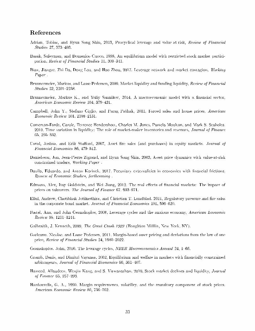
References

Adrian, Tobias, and Hyun Song Shin, 2013, Procyclical leverage and value-at-risk, Review of Financial

Studies 27, 373�403.

Basak, Suleyman, and Domenico Cuoco, 1998, An equilibrium model with restricted stock market partici-pation, Review of Financial Studies 11, 309�341.

Bian, Jiangze, Zhi Da, Dong Lou, and Hao Zhou, 2017, Leverage network and market contagion, Working

Paper .

Brunnermeier, Markus, and Lasse Pedersen, 2009, Market liquidity and funding liquidity, Review of Financial

Studies 22, 2201�2238.

Brunnermeier, Markus K., and Yuliy Sannikov, 2014, A macroeconomic model with a �nancial sector,American Economic Review 104, 379�421.

Campbell, John Y., Stefano Giglio, and Parag Pathak, 2011, Forced sales and house prices, AmericanEconomic Review 101, 2108�2131.

Comerton-Forde, Carole, Terrence Hendershott, Charles M. Jones, Pamela Moulton, and Mark S. Seaholes,2010, Time variation in liquidity: The role of market-maker inventories and revenues, Journal of Finance65, 295�332.

Coval, Joshua, and Erik Sta�ord, 2007, Asset �re sales (and purchases) in equity markets, Journal ofFinancial Economics 86, 479�512.

Danielsson, Jon, Jean-Pierre Zigrand, and Hyun Song Shin, 2002, Asset price dynamics with value-at-riskconstrained traders, Working Paper .

Davila, Eduardo, and Anton Korinek, 2017, Pecuniary externalities in economies with �nancial frictions,Review of Economic Studies, forthcoming .

Edmans, Alex, Itay Goldstein, and Wei Jiang, 2012, The real e�ects of �nancial markets: The impact ofprices on takeovers, The Journal of Finance 67, 933�971.

Ellul, Andrew, Chotibhak Jotikasthira, and Christian T. Lundblad, 2011, Regulatory pressure and �re salesin the corporate bond market, Journal of Financial Economics 101, 596�620.

Fostel, Ana, and John Geanakoplos, 2008, Leverage cycles and the anxious economy, American Economic

Review 98, 1211�1244.

Galbraith, J. Kenneth, 2009, The Great Crash 1929 (Houghton Mi�in, New York, NY).

Garleanu, Nicolae, and Lasse Pedersen, 2011, Margin-based asset pricing and deviations from the law of oneprice, Review of Financial Studies 24, 1980�2022.

Geanakoplos, John, 2010, The leverage cycles, NBER Macroeconomics Annual 24, 1�66.

Gromb, Denis, and Dimitri Vayanos, 2002, Equilibrium and welfare in markets with �nancially constrainedarbitrageurs, Journal of Financial Economics 66, 361�407.

Hameed, Allaudeen, Wenjin Kang, and S. Viswanathan, 2010, Stock market declines and liquidity, Journalof Finance 65, 257�293.

Hardouvelis, G. A., 1990, Margin requirements, volatility, and the transitory component of stock prices,American Economic Review 80, 736�762.

33

Hardouvelis, Gikas A., and Panayiotis Theodossiou, 2002, The asymmetric relation between initial marginrequirements and stock market volatility across bull and bear markets, Review of Financial Studies 15,1525�1559.

He, Zhiguo, Bryan Kelly, and Asaf Manela, 2017, Intermediary asset pricing: New evidence from many assetclasses, Journal of Financial Economics, Forthcoming .

He, Zhiguo, and Peter Kondor, 2016, Ine�cient investment waves, Econometrica 84, 735�780.

He, Zhiguo, and Arvind Krishnamurthy, 2013, Intermediary asset pricing, American Economic Review 103,732�770.

Huang, Yi, Jianjun Miao, and Pengfei Wang, 2016, Saving china's stock market, Working Paper .

Kyle, Albert S, and Wei Xiong, 2001, Contagion as a wealth e�ect, Journal of Finance 56, 1401�1440.

Lorenzoni, Guido, 2008, Ine�cient credit booms, Review of Economic Studies 75, 809�833.

Mian, Atif, Kamalesh Rao, and Amir Su�, 2013, Household balance sheets, consumption, and the economicslump, The Quarterly Journal of Economics 128, 1687�1726.

Mitchell, Mark, Lasse Pedersen, and Todd Pulvino, 2007, Slow moving capital, American Economic Review,

Papers and Proceedings 97, 215�220.

Pulvino, Todd, 1998, Do asset �re sales exist? an empirical investigation of commercial aircraft transactions,Journal of Finance 53, 939�978.

Schwert, G. William, 1989, Margin requirements and stock volatility, Journal of Financial Services Research3, 153�164.

Shleifer, Andrei, and Robert Vishny, 1992, Liquidation values and debt capacity: a market equilibriumapproach, Journal of Finance 47, 1343�1366.

Stein, Jeremy C., 2012, Monetary policy as �nancial-stability regulation, Quarterly Journal of Economics

127, 57�95.

Tookes, Heather E., and Bige Kahraman, 2016, Trader leverage and liquidity, Journal of Finance, forthcoming.

34

Figure 1Structure and Funding Sources of Margin Systems in the Chinese Stock Market

This �gure depicts the structure and funding sources in the brokerage- and shadow-�nanced margin systemsin the Chinese stock market.

Figure 1. Structure and funding sources in Brokerage and Shadow-financed margin system in Chinese stock market.

Brokerage Firms' own

Capital

Regulated Brokerage-Financed System

Credit from CSFC

WMP from Commercial

Banks

Trust and P2P via Informal

Lending

Pledged Stock Rights

Unregulated Shadow-Financed System

Connected to Broker Accounts to Trade Stocks

35

Figure 2Leverage for Brokerage and Shadow Accounts

This �gure depicts the Shanghai Stock Exchange (SSE) composite index (the dashed blue line), the averageleverage for shadow margin accounts (the solid red line), and the average leverage for brokerage marginaccounts (the dashed-dotted red line), weighted by the equity size of each account, at the end of each dayfrom May to July, 2015. To compute the average, we weight each account's leverage by the equity in eachaccount. Weighted in this manner, average leverage equals total debt scaled by total assets.

36

Figure 3Asset-Weighted and Equity-Weighted Leverage

This �gure depicts the Shanghai Stock Exchange (SSE) composite index (the dashed blue line), the asset-weighted average leverage for all margin accounts (the solid red line), and the equity-weighted averageleverage for all margin accounts (the dashed-dotted red line), at the end of each day from May to July, 2015.To compute the averages, we weight each account's leverage by the assets or equity in each account.

37

Figure 4Leverage Dispersion

This �gure depicts the Shanghai Stock Exchange (SSE) composite index (the dashed blue line) and themargin account leverage at the 20th (dashed-dotted red line), 50th (dashed red line), and 80th (solid redline) percentiles of the full sample including both brokerage- and shadow-�nanced margin accounts, at theend of each day from May to July, 2015.

38

Figure 5Proximity to the Pingcang Line and Investor Selling Intensity

This �gure plots the coe�cients λk of the regression equation

δjit =

11∑k=1

λkIjk,t−1 + νit + αj + εjit

where δjjt is account j's net selling volume of stock i on day t, normalized by account j's initial holdingof stock i at the beginning of day t. νit is the stock-date �xed e�ect and αj is the account �xed e�ect.

Ijk,t−1 represents 10 equally spaced bins for each account's proximity to its Pingcang Line. Accounts withleverage exceeding the Pingcang Line are assigned to bin 11. Unleveraged accounts are the omitted category.The sample includes all brokerage- and shadow-�nanced margin accounts, as well as brokerage non-marginaccounts which aid in the estimation of the omitted category. The time period is from May to July, 2015.

39

Figure 6Proximity to the Pingcang Line and Investor Selling Intensity: Market Returns

This �gure plots the the coe�cients λk from the regression de�ned in Figure 5, estimated separately for thesamples in which the market return on day t is positive and negative. The time period is from May to July,2015.

40

Figure 7Returns Following Fire Sales: Long-Short Portfolio

This �gure plots the average long-short portfolio cumulative abnormal return after double sorts based oneach stock's previous period return and �re sale exposure (FSE). On each day t, we sort all stocks held by�re sale accounts into four quartiles according to their return over the period [t − 10, t − 1]. Within eachquartile, we then sort stocks into 10 bins according to their FSE at the start of each day t. For each quartileof previous period returns, we construct a long-short strategy that longs the bin with the highest FSE andshorts the bin with the lowest FSE. The sample includes all stocks held by brokerage- and shadow-�nancedmargin accounts. The time period is from May to July, 2015.

41

Figure 8Proximity to the Pingcang Line and Investor Selling Intensity: Brokerage and Shadow

Accounts

This �gure plots the the coe�cients λk from the regression de�ned in Figure 5, estimated separately for thebrokerage- and shadow-�nanced margin account samples. The time period is from May to July, 2015.

42

Figure 9Regulatory Tightening

Regulatory tightening announcements occurred after hours on Friday May 22, 2015 and Friday June 12,2015. This �gure plots the coe�cients λk from the regression de�ned in Figure 5, estimated separately forthe brokerage- and shadow-�nanced margin account samples for the �ve trading days immediately beforeand after the regulatory tightening events.

43

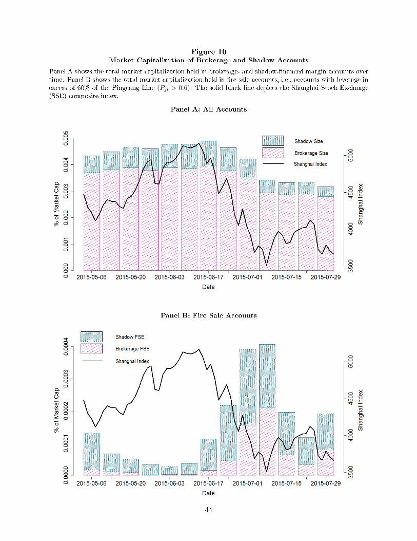
Figure 10Market Capitalization of Brokerage and Shadow Accounts

Panel A shows the total market capitalization held in brokerage- and shadow-�nanced margin accounts overtime. Panel B shows the total market capitalization held in �re sale accounts, i.e., accounts with leverage inexcess of 60% of the Pingcang Line (Pjt > 0.6). The solid black line depicts the Shanghai Stock Exchange(SSE) composite index.

Panel A: All Accounts

Panel B: Fire Sale Accounts

44

Table 1Summary Statistics

This table presents summary statistics for account activity and stocks characteristics from May to July 2015.Leverage is the ratio of assets to equity at the end of each account-day, where equity is equal to assets minusdebt. The Pingcang Line is the account-level maximum allowable level of leverage. Proximity is the ratio ofleverage minus 1 to the Pingcang Line minus 1. An account is classi�ed as a �re sale account on day t if theproximity to the Pingcang Line exceeds 0.6. Net selling is account j's net selling volume of stock i on day t,normalized by account j's shares held of stock i at the beginning of day t. Selling pressure is the total netselling volume of stock i on day t from all �re sale accounts that hold stock i at the start of day t, scaledby the number of outstanding shares of stock i at the beginning of day t. Fire sale exposure is the ratioof the total shares of stock i held in �re sale accounts at the start of day t to the number of outstandingshares of stock i on day t. CAR is the cumulative abnormal return estimated relative to the CAPM, withbeta calculated for each stock using year 2014 data. Return volatility is the standard deviation of returnsduring the prior 60 days. Log market value is the log of the product of each stock's daily close price andtotal number of shares outstanding, measured in t − 3. Avg turnover is the average of the ratio of tradingvolume in shares to the total shares outstanding in the prior 60 days.

Panel A: Account-Day Level

Mean S.D. Min p25 p50 p75 Max ObsLeverage, full sample 1.1246 1.972186 1 1 1 1 100 114669566Leverage, shadow accounts 6.61317 12.72582 1 3.041404 4.304326 6.001816 100 2308393Leverage, brokerage accounts 1.42792 0.457916 1 1 1.350877 1.694444 51 3109096Leverage, non-margin accounts 1 0 1 1 1 1 1 109252077Pingcang Line, full sample 1.300731 1.732132 1 1 1 1 100 114669566Pingcang Line, shadow accounts 11.49418 5.360652 2 10 10 11.0011 100 2308393Pingcang Line, brokerage accounts 4.3 0 4.3 4.3 4.3 4.3 4.3 3109096Pingcang Line, non-margin accounts 1 0 1 1 1 1 1 109252077Proximity, full sample 0.320911 0.959172 0 0.054673 0.189394 0.3367 79.9911 5417489Proximity, shadow accounts 0.578482 1.420425 0 0.202023 0.33558 0.512729 79.9911 2308393Proximity, brokerage accounts 0.129673 0.138762 0 0 0.106326 0.210438 15.1515 3109096Proximity, non-margin accounts 0 0 0 0 0 0 0 109252077Account assets, full sample 3050874 26988688 0.02 174375.6 602996.9 1788544 4.5E+09 5417489Account assets, shadow accounts 1517140 6192097 0.02 60290 215769.3 753314.2 5.1E+08 2308393Account assets, brokerage accounts 4189618 35180700 3.85 429573.3 995861.4 2494273 4.5E+09 3109096

Mean S.D. Min p25 p50 p75 Max ObsNet selling, full sample 0.074041 0.315285 -1.2 0 0 0 1 351403587Net selling, shadow accounts 0.223761 0.454715 -1.2 0 0 0.5 1 6227811Net selling, brokerage accounts 0.085903 0.33442 -1.2 0 0 0 1 16658787Net selling, non-margin accounts 0.070601 0.310314 -1.2 0 0 0 1 328516989

Mean S.D. Min p25 p50 p75 Max ObsSelling pressure, all margin accounts 0.000017 0.000202 -0.005028 -0.000004 0.000000 0.000011 0.025943 116809Selling pressure, shadow accounts 0.000012 0.000170 -0.005028 -0.000004 0.000000 0.000010 0.025943 116809Selling pressure, brokerage accounts 0.000005 0.000106 -0.002344 0.000000 0.000000 0.000000 0.019551 116809Fire sale exposure, all margin accounts 0.000204 0.000771 0.000000 0.000006 0.000036 0.000149 0.053907 116809Fire sale exposure, shadow accounts 0.000153 0.000569 0.000000 0.000005 0.000030 0.000117 0.053907 116809Fire sale exposure, brokerage accounts 0.000051 0.000491 0.000000 0.000000 0.000000 0.000000 0.053271 116809CAR [t] -0.0003 0.0417 -0.1824 -0.0270 -0.0036 0.0245 0.2164 109735CAR [t,t+3] -0.0014 0.0820 -0.3971 -0.0500 -0.0038 0.0457 0.5344 109735CAR [t,t+5] -0.0016 0.1097 -0.5303 -0.0635 -0.0014 0.0634 0.5425 109735CAR [t,t+10] 0.0006 0.1575 -0.7929 -0.0851 0.0089 0.0957 0.7455 109735CAR [t,t+20] 0.0004 0.2030 -1.0486 -0.1235 0.0117 0.1292 1.1256 109735CAR [t,t+40] -0.0207 0.2003 -1.1560 -0.1473 -0.0200 0.1015 1.1301 109735Cumulative return [t-10,t-1] 1.0370 0.2404 0.3308 0.8977 1.0409 1.1795 2.6483 116809Return volatility [t-60, t-1] 0.0442 0.0128 0.0000 0.0343 0.0424 0.0532 0.1016 116809Log market value [t-3] 9.47 0.98 7.36 8.78 9.29 9.97 14.78 116809Avg turnover [t-60,t-1] 0.0494 0.0257 0.0002 0.0314 0.0449 0.0624 0.2446 116809

Panel B: Account-Stock-Day Level

Mean S.D. Min p25 p50 p75 Max ObsLeverage, full sample 1.1246 1.972186 1 1 1 1 100 114669566Leverage, shadow accounts 6.61317 12.72582 1 3.041404 4.304326 6.001816 100 2308393Leverage, brokerage accounts 1.42792 0.457916 1 1 1.350877 1.694444 51 3109096Leverage, non-margin accounts 1 0 1 1 1 1 1 109252077Pingcang Line, full sample 1.300731 1.732132 1 1 1 1 100 114669566Pingcang Line, shadow accounts 11.49418 5.360652 2 10 10 11.0011 100 2308393Pingcang Line, brokerage accounts 4.3 0 4.3 4.3 4.3 4.3 4.3 3109096Pingcang Line, non-margin accounts 1 0 1 1 1 1 1 109252077Proximity, full sample 0.320911 0.959172 0 0.054673 0.189394 0.3367 79.9911 5417489Proximity, shadow accounts 0.578482 1.420425 0 0.202023 0.33558 0.512729 79.9911 2308393Proximity, brokerage accounts 0.129673 0.138762 0 0 0.106326 0.210438 15.1515 3109096Proximity, non-margin accounts 0 0 0 0 0 0 0 109252077Account assets, full sample 3050874 26988688 0.02 174375.6 602996.9 1788544 4.5E+09 5417489Account assets, shadow accounts 1517140 6192097 0.02 60290 215769.3 753314.2 5.1E+08 2308393Account assets, brokerage accounts 4189618 35180700 3.85 429573.3 995861.4 2494273 4.5E+09 3109096

Mean S.D. Min p25 p50 p75 Max ObsNet selling, full sample 0.074041 0.315285 -1.2 0 0 0 1 351403587Net selling, shadow accounts 0.223761 0.454715 -1.2 0 0 0.5 1 6227811Net selling, brokerage accounts 0.085903 0.33442 -1.2 0 0 0 1 16658787Net selling, non-margin accounts 0.070601 0.310314 -1.2 0 0 0 1 328516989

Mean S.D. Min p25 p50 p75 Max ObsSelling pressure, all margin accounts 0.000017 0.000202 -0.005028 -0.000004 0.000000 0.000011 0.025943 116809Selling pressure, shadow accounts 0.000012 0.000170 -0.005028 -0.000004 0.000000 0.000010 0.025943 116809Selling pressure, brokerage accounts 0.000005 0.000106 -0.002344 0.000000 0.000000 0.000000 0.019551 116809Fire sale exposure, all margin accounts 0.000204 0.000771 0.000000 0.000006 0.000036 0.000149 0.053907 116809Fire sale exposure, shadow accounts 0.000153 0.000569 0.000000 0.000005 0.000030 0.000117 0.053907 116809Fire sale exposure, brokerage accounts 0.000051 0.000491 0.000000 0.000000 0.000000 0.000000 0.053271 116809CAR [t] -0.0003 0.0417 -0.1824 -0.0270 -0.0036 0.0245 0.2164 109735CAR [t,t+3] -0.0014 0.0820 -0.3971 -0.0500 -0.0038 0.0457 0.5344 109735CAR [t,t+5] -0.0016 0.1097 -0.5303 -0.0635 -0.0014 0.0634 0.5425 109735CAR [t,t+10] 0.0006 0.1575 -0.7929 -0.0851 0.0089 0.0957 0.7455 109735CAR [t,t+20] 0.0004 0.2030 -1.0486 -0.1235 0.0117 0.1292 1.1256 109735CAR [t,t+40] -0.0207 0.2003 -1.1560 -0.1473 -0.0200 0.1015 1.1301 109735Cumulative return [t-10,t-1] 1.0370 0.2404 0.3308 0.8977 1.0409 1.1795 2.6483 116809Return volatility [t-60, t-1] 0.0442 0.0128 0.0000 0.0343 0.0424 0.0532 0.1016 116809Log market value [t-3] 9.47 0.98 7.36 8.78 9.29 9.97 14.78 116809Avg turnover [t-60,t-1] 0.0494 0.0257 0.0002 0.0314 0.0449 0.0624 0.2446 116809

45

Table 1Summary Statistics (Continued)

Panel C: Stock-Day Level

Mean S.D. Min p25 p50 p75 Max ObsLeverage, full sample 1.1246 1.972186 1 1 1 1 100 114669566Leverage, shadow accounts 6.61317 12.72582 1 3.041404 4.304326 6.001816 100 2308393Leverage, brokerage accounts 1.42792 0.457916 1 1 1.350877 1.694444 51 3109096Leverage, non-margin accounts 1 0 1 1 1 1 1 109252077Pingcang Line, full sample 1.300731 1.732132 1 1 1 1 100 114669566Pingcang Line, shadow accounts 11.49418 5.360652 2 10 10 11.0011 100 2308393Pingcang Line, brokerage accounts 4.3 0 4.3 4.3 4.3 4.3 4.3 3109096Pingcang Line, non-margin accounts 1 0 1 1 1 1 1 109252077Proximity, full sample 0.320911 0.959172 0 0.054673 0.189394 0.3367 79.9911 5417489Proximity, shadow accounts 0.578482 1.420425 0 0.202023 0.33558 0.512729 79.9911 2308393Proximity, brokerage accounts 0.129673 0.138762 0 0 0.106326 0.210438 15.1515 3109096Proximity, non-margin accounts 0 0 0 0 0 0 0 109252077Account assets, full sample 3050874 26988688 0.02 174375.6 602996.9 1788544 4.5E+09 5417489Account assets, shadow accounts 1517140 6192097 0.02 60290 215769.3 753314.2 5.1E+08 2308393Account assets, brokerage accounts 4189618 35180700 3.85 429573.3 995861.4 2494273 4.5E+09 3109096

Mean S.D. Min p25 p50 p75 Max ObsNet selling, full sample 0.074041 0.315285 -1.2 0 0 0 1 351403587Net selling, shadow accounts 0.223761 0.454715 -1.2 0 0 0.5 1 6227811Net selling, brokerage accounts 0.085903 0.33442 -1.2 0 0 0 1 16658787Net selling, non-margin accounts 0.070601 0.310314 -1.2 0 0 0 1 328516989

Mean S.D. Min p25 p50 p75 Max ObsSelling pressure, all margin accounts 0.000017 0.000202 -0.005028 -0.000004 0.000000 0.000011 0.025943 116809Selling pressure, shadow accounts 0.000012 0.000170 -0.005028 -0.000004 0.000000 0.000010 0.025943 116809Selling pressure, brokerage accounts 0.000005 0.000106 -0.002344 0.000000 0.000000 0.000000 0.019551 116809Fire sale exposure, all margin accounts 0.000204 0.000771 0.000000 0.000006 0.000036 0.000149 0.053907 116809Fire sale exposure, shadow accounts 0.000153 0.000569 0.000000 0.000005 0.000030 0.000117 0.053907 116809Fire sale exposure, brokerage accounts 0.000051 0.000491 0.000000 0.000000 0.000000 0.000000 0.053271 116809CAR [t] -0.0003 0.0417 -0.1824 -0.0270 -0.0036 0.0245 0.2164 109735CAR [t,t+3] -0.0014 0.0820 -0.3971 -0.0500 -0.0038 0.0457 0.5344 109735CAR [t,t+5] -0.0016 0.1097 -0.5303 -0.0635 -0.0014 0.0634 0.5425 109735CAR [t,t+10] 0.0006 0.1575 -0.7929 -0.0851 0.0089 0.0957 0.7455 109735CAR [t,t+20] 0.0004 0.2030 -1.0486 -0.1235 0.0117 0.1292 1.1256 109735CAR [t,t+40] -0.0207 0.2003 -1.1560 -0.1473 -0.0200 0.1015 1.1301 109735Cumulative return [t-10,t-1] 1.0370 0.2404 0.3308 0.8977 1.0409 1.1795 2.6483 116809Return volatility [t-60, t-1] 0.0442 0.0128 0.0000 0.0343 0.0424 0.0532 0.1016 116809Log market value [t-3] 9.47 0.98 7.36 8.78 9.29 9.97 14.78 116809Avg turnover [t-60,t-1] 0.0494 0.0257 0.0002 0.0314 0.0449 0.0624 0.2446 116809

46

Table 2Proximity to the Pingcang Line and Investor Selling Intensity

This table shows the coe�cients λk of the regression equation

δjit =

11∑k=1

λkIjk,t−1 + νit + αj + εjit

where δjjt is account j's net selling volume of stock i on day t, normalized by account j's initial holdingof stock i at the beginning of day t. νit is the stock-date �xed e�ect and αj is the account �xed e�ect.

Ijk,t−1 represents 10 equally spaced bins for each account's proximity to its Pingcang Line. Accounts withleverage exceeding the Pingcang Line are assigned to bin 11. Unleveraged accounts are the omitted category.The sample includes all brokerage- and shadow-�nanced margin accounts, as well as brokerage non-marginaccounts which comprise the omitted category. The time period is from May to July, 2015. Standard errorsare allowed to be clustered at the account-date level. ***, **, * correspond to statistical signi�cance at the1%, 5%, and 10% levels, respectively.Baseline

Net selling Full Broker Shadow(1) (2) (3)

Proximity in (0/10, 1/10) -0.00398*** -0.00429*** 0.00459(0.000396) (0.000407) (0.00283)

Proximity in [1/10, 2/10) -0.000281 -0.000108 0.00212(0.000329) (0.000341) (0.00288)

Proximity in [2/10, 3/10) 0.00426*** 0.00565*** 0.00346(0.000368) (0.000392) (0.00290)

Proximity in [3/10, 4/10) 0.00595*** 0.00917*** 0.00639**(0.000483) (0.000567) (0.00292)

Proximity in [4/10, 5/10) 0.0119*** 0.0113*** 0.0168***(0.000684) (0.00106) (0.00295)

Proximity in [5/10, 6/10) 0.0356*** 0.0153*** 0.0465***(0.000906) (0.00152) (0.00302)

Proximity in [6/10, 7/10) 0.0734*** 0.0327*** 0.0872***(0.00119) (0.00216) (0.00312)

Proximity in [7/10, 8/10) 0.112*** 0.0518*** 0.129***(0.00156) (0.00313) (0.00330)

Proximity in [8/10, 9/10) 0.151*** 0.0743*** 0.167***(0.00207) (0.00474) (0.00357)

Proximity in [9/10, 10/10) 0.183*** 0.108*** 0.198***(0.00270) (0.0102) (0.00396)

Proximity >= 1 0.188*** 0.214*** 0.194***(0.00149) (0.00953) (0.00319)

Account FE Yes Yes YesStock-Date FE Yes Yes YesR-squared 0.140 0.135 0.141Observations 351,389,311 345,167,235 334,729,975

47

Table 3Proximity and Leverage Interactions

This table examines how leverage levels and proximity to the Pingcang Line impact net selling. The sampleis restricted to shadow-�nanced margin accounts. Column 1 replicates Column 3 of Table 2. Column 2 addscontrols for �ve bins representing leverage at the start of of each account-day and the interaction between theleverage bins and an indicator for whether the account is considered a �re sale account. The leverage bins arespaced so that the number of observations in proximity bins b and b+1 equal to the number of observationsin leverage bin (b+ 1)/2, for b = 1, 2, ..., 10. Standard errors are allowed to be clustered at the account-datelevel. ***, **, * correspond to statistical signi�cance at the 1%, 5%, and 10% levels, respectively.

Net selling (1) (2)Proximity in (0/10, 1/10) 0.00459 0.00960***

(0.00283) (0.00284)Proximity in [1/10, 2/10) 0.00212 0.0193***

(0.00288) (0.00313)Proximity in [2/10, 3/10) 0.00346 0.0276***

(0.00290) (0.00321)Proximity in [3/10, 4/10) 0.00639** 0.0349***

(0.00292) (0.00327)Proximity in [4/10, 5/10) 0.0168*** 0.0444***

(0.00295) (0.00339)Proximity in [5/10, 6/10) 0.0465*** 0.0670***

(0.00302) (0.00347)Proximity in [6/10, 7/10) 0.0872*** 0.0958***

(0.00312) (0.00603)Proximity in [7/10, 8/10) 0.129*** 0.120***

(0.00330) (0.00601)Proximity in [8/10, 9/10) 0.167*** 0.143***

(0.00357) (0.00610)Proximity in [9/10, 10/10) 0.198*** 0.161***

(0.00396) (0.00639)Proximity >= 1 0.194*** 0.132***

(0.00319) (0.00650)Lev Bin 1 -0.0181***

(0.00160)Lev Bin 2 -0.0107***

(0.000791)Lev Bin 3 -0.0278***

(0.00171)Lev Bin 4 -0.00105

(0.00103)Lev Bin 5 0.0290***

(0.00508)Lev Bin 1 * 1{Proximity >= 0.6} -0.00437

(0.00695)Lev Bin 2 * 1{Proximity >= 0.6} -0.0172***

(0.00365)Lev Bin 3 * 1{Proximity >= 0.6} -0.0102***

(0.00285)Lev Bin 4 * 1{Proximity >= 0.6} 0.0167***

(0.00497)Lev Bin 5 * 1{Proximity >= 0.6} 0.0286***

(0.00747)Account FE Yes YesStock-Date FE Yes YesR-squared 0.141 0.141Observations 334,729,975 334,729,975

48

Table 4Investor Selling Intensity Conditional on Day t Market Returns

Panels A and B present the same regression as in Table 4, with the sample restricted days in which the marketreturn was positive or negative, respectively Standard errors are allowed to be clustered at the account-datelevel. ***, **, * correspond to statistical signi�cance at the 1%, 5%, and 10% levels, respectively.

Panel A: Positive Market Return Day

Market Up Ex Post

Net selling Full Broker Shadow(1) (2) (3)

Proximity in (0/10, 1/10) -0.00248*** -0.00311*** 0.0211***(0.000515) (0.000528) (0.00367)

Proximity in [1/10, 2/10) -0.000952** -0.00119*** 0.0166***(0.000426) (0.000442) (0.00375)

Proximity in [2/10, 3/10) -0.00102** -0.000371 0.0133***(0.000492) (0.000530) (0.00378)

Proximity in [3/10, 4/10) -0.00336*** -0.00120* 0.0106***(0.000629) (0.000723) (0.00381)

Proximity in [4/10, 5/10) -0.00260*** -0.000249 0.0125***(0.000875) (0.00127) (0.00385)

Proximity in [5/10, 6/10) 0.00653*** -0.00156 0.0253***(0.00113) (0.00165) (0.00394)

Proximity in [6/10, 7/10) 0.0256*** 0.00866*** 0.0459***(0.00152) (0.00298) (0.00408)

Proximity in [7/10, 8/10) 0.0472*** 0.0203*** 0.0692***(0.00196) (0.00303) (0.00432)

Proximity in [8/10, 9/10) 0.0711*** 0.0324*** 0.0927***(0.00256) (0.00627) (0.00460)

Proximity in [9/10, 10/10) 0.0956*** 0.0465*** 0.118***(0.00361) (0.00760) (0.00536)

Proximity >= 1 0.115*** 0.197*** 0.129***(0.00198) (0.0136) (0.00418)

Account FE Yes Yes YesStock-Date FE Yes Yes YesR-squared 0.155 0.150 0.159Observations 181,307,544 178,031,345 172,673,737

Market Down Ex Post

49

Table 4Investor Selling Intensity Conditional on Day t Market Returns (Continued)

Panel B: Negative Market Return Day

Net selling Full Broker Shadow(1) (2) (3)

Proximity in (0/10, 1/10) -0.00587*** -0.00583*** -0.0123***(0.000548) (0.000560) (0.00422)

Proximity in [1/10, 2/10) 0.00116*** 0.00200*** -0.0137***(0.000449) (0.000462) (0.00429)

Proximity in [2/10, 3/10) 0.0107*** 0.0127*** -0.00565(0.000492) (0.000515) (0.00432)

Proximity in [3/10, 4/10) 0.0164*** 0.0194*** 0.00388(0.000683) (0.000797) (0.00435)

Proximity in [4/10, 5/10) 0.0290*** 0.0243*** 0.0237***(0.000995) (0.00154) (0.00439)

Proximity in [5/10, 6/10) 0.0657*** 0.0342*** 0.0681***(0.00135) (0.00239) (0.00449)

Proximity in [6/10, 7/10) 0.119*** 0.0600*** 0.124***(0.00172) (0.00297) (0.00463)

Proximity in [7/10, 8/10) 0.171*** 0.0887*** 0.180***(0.00222) (0.00496) (0.00486)

Proximity in [8/10, 9/10) 0.219*** 0.112*** 0.226***(0.00308) (0.00746) (0.00525)

Proximity in [9/10, 10/10) 0.257*** 0.164*** 0.263***(0.00359) (0.0126) (0.00563)

Proximity >= 1 0.251*** 0.231*** 0.247***(0.00208) (0.0121) (0.00469)

Account FE Yes Yes YesStock-Date FE Yes Yes YesR-squared 0.152 0.145 0.152Observations 170,051,679 167,114,226 162,025,214

50

Table 5Stock-Level Fire Sale Exposure and Selling Pressure

This table presents the regression

δit = β · FSEit + controlsit + si + τt + εit.

δit measures stock-level selling pressure from �re sale account. FSEit is the �re sale exposure for stock i onday t. δit and FSEit are calculated using the combined brokerage and shadow account samples in Panel A,the brokerage account sample in Panel B and the shadow account sample in Panel C. All variables are asde�ned in Table 1. Standard errors are allowed to be clustered at the date level. ***, **, * correspond tostatistical signi�cance at the 1%, 5%, and 10% levels, respectively.

Panel A: FSE Calculated Using All Margin AccountsBaseline

(1) (2) (3) (4)

Fire sale exposure 0.0996*** 0.102*** 0.102*** 0.102***(0.0221) (0.0259) (0.0259) (0.0259)

Return volatility [t-60, t-1] -0.000370* -0.000273(0.000190) (0.000187)

Log market value [t-3] 2.40e-05*** 1.33e-05(7.10e-06) (7.95e-06)

Avg turnover [t-60, t-1] 2.11e-05 3.67e-05(0.000169) (0.000175)

Cumulative return [t-10, t-1] -2.25e-05*** 4.28e-05**(5.51e-06) (1.71e-05)

Stock FE No Yes Yes YesDate FE No Yes Yes YesPast 10-day daily returns No No No YesR-squared 0.144 0.186 0.186 0.187Observations 116,809 116,809 116,809 116,809

Broker

(1) (2) (3) (4)

Fire sale exposure 0.0756*** 0.0747*** 0.0747*** 0.0746***(0.0153) (0.0156) (0.0157) (0.0157)

Return volatility [t-60, t-1] -0.000176* -0.000145(9.81e-05) (9.91e-05)

Log market value [t-3] -3.36e-06 -2.46e-06(3.07e-06) (3.40e-06)

Avg turnover [t-60, t-1] 9.27e-05 9.08e-05(7.24e-05) (7.38e-05)

Cumulative return [t-10, t-1] -6.11e-07 1.92e-05(1.80e-06) (1.16e-05)

Stock FE No Yes Yes YesDate FE No Yes Yes YesPast 10-day daily returns No No No YesR-squared 0.122 0.151 0.151 0.151Observations 116,809 116,809 116,809 116,809

Selling pressure

Selling pressure

51

Table 5Stock-Level Fire Sale Exposure and Selling Pressure (Continued)

Panel B: FSE Calculated Using Brokerage Margin Accounts

Baseline

(1) (2) (3) (4)

Fire sale exposure 0.0996*** 0.102*** 0.102*** 0.102***(0.0221) (0.0259) (0.0259) (0.0259)

Return volatility [t-60, t-1] -0.000370* -0.000273(0.000190) (0.000187)

Log market value [t-3] 2.40e-05*** 1.33e-05(7.10e-06) (7.95e-06)

Avg turnover [t-60, t-1] 2.11e-05 3.67e-05(0.000169) (0.000175)

Cumulative return [t-10, t-1] -2.25e-05*** 4.28e-05**(5.51e-06) (1.71e-05)

Stock FE No Yes Yes YesDate FE No Yes Yes YesPast 10-day daily returns No No No YesR-squared 0.144 0.186 0.186 0.187Observations 116,809 116,809 116,809 116,809

Broker

(1) (2) (3) (4)

Fire sale exposure 0.0756*** 0.0747*** 0.0747*** 0.0746***(0.0153) (0.0156) (0.0157) (0.0157)

Return volatility [t-60, t-1] -0.000176* -0.000145(9.81e-05) (9.91e-05)

Log market value [t-3] -3.36e-06 -2.46e-06(3.07e-06) (3.40e-06)

Avg turnover [t-60, t-1] 9.27e-05 9.08e-05(7.24e-05) (7.38e-05)

Cumulative return [t-10, t-1] -6.11e-07 1.92e-05(1.80e-06) (1.16e-05)

Stock FE No Yes Yes YesDate FE No Yes Yes YesPast 10-day daily returns No No No YesR-squared 0.122 0.151 0.151 0.151Observations 116,809 116,809 116,809 116,809

Selling pressure

Selling pressure

Panel C: FSE Calculated Using Shadow Margin AccountsShadow

(1) (2) (3) (4)

Fire sale exposure 0.113*** 0.125*** 0.124*** 0.124***(0.0341) (0.0417) (0.0418) (0.0418)

Return volatility [t-60, t-1] -0.000109 -3.68e-05(0.000167) (0.000163)

Log market value [t-3] 2.00e-05** 8.97e-06(8.66e-06) (7.18e-06)

Avg turnover [t-60, t-1] -0.000108 -9.08e-05(0.000142) (0.000147)

Cumulative return [t-10, t-1] -1.91e-05*** 3.15e-05**(7.14e-06) (1.40e-05)

Stock FE No Yes Yes YesDate FE No Yes Yes YesPast 10-day daily returns No No No YesR-squared 0.144 0.189 0.189 0.191Observations 116,809 116,809 116,809 116,809

Baseline, Lambda weighted

(1) (2) (3) (4)

Fire sale exposure 0.874*** 0.957*** 0.961*** 0.980***(0.149) (0.193) (0.192) (0.193)

Return volatility [t-60, t-1] 0.00381*** 0.00386***(0.00138) (0.00136)

Log market value [t-3] 0.000117*** 0.000241***(3.53e-05) (4.17e-05)

Avg turnover [t-60, t-1] 0.00184** 0.00161**(0.000777) (0.000768)

Cumulative return [t-10, t-1] 0.000183*** 0.000227**(4.37e-05) (0.000110)

Stock FE No Yes Yes YesDate FE No Yes Yes YesPast 10-day daily returns No No No YesR-squared 0.010 0.029 0.030 0.031Observations 116,809 116,809 116,809 116,809

Selling pressure

Selling pressure

52

Table 6Fire Sales and Reversals

The table presents the regression

CARi,t+h = γh · FSEit + controlsit + si + τt + εit.

All variables are as de�ned in Table 1. Standard errors are allowed to be clustered at the date level. ***,**, * correspond to statistical signi�cance at the 1%, 5%, and 10% levels, respectively.

Panel A: FSE Calculated Using All Margin AccountsFull

CAR: [t] [t, t+3] [t, t+5] [t, t+10] [t, t+20] [t, t+40](1) (2) (3) (4) (5) (6)

Fire sale exposure -1.422*** -3.529*** -5.089*** -5.924*** -2.827*** 0.290(0.312) (0.594) (0.910) (1.264) (0.924) (0.570)

Return volatility [t-60, t-1] -0.172 -0.300 -0.356 -0.319 0.466 0.161(0.148) (0.313) (0.389) (0.491) (0.540) (0.353)

Log market value [t-3] -0.0652*** -0.201*** -0.322*** -0.568*** -0.822*** -0.745***(0.00749) (0.0144) (0.0198) (0.0288) (0.0308) (0.0196)

Avg turnover [t-60, t-1] -0.0809 -0.248* -0.436*** -0.888*** -2.017*** -1.236***(0.0685) (0.125) (0.154) (0.159) (0.177) (0.143)

Cumulative return [t-10, t-1] -0.0230 -0.0330 -0.0284 0.0356 -0.0450 0.102***(0.0146) (0.0285) (0.0393) (0.0489) (0.0465) (0.0271)

Date FE Yes Yes Yes Yes Yes Yes Stock FE Yes Yes Yes Yes Yes Yes Past 10-day daily return Yes Yes Yes Yes Yes Yes R-squared 0.254 0.354 0.415 0.538 0.653 0.730Observations 109,735 109,735 109,735 109,735 109,735 109,735

Brokerage

CAR: [t] [t, t+3] [t, t+5] [t, t+10] [t, t+20] [t, t+40](1) (2) (3) (4) (5) (6)

Fire sale exposure -0.621*** -1.519*** -1.829*** -1.052 -2.170*** 0.0725(0.222) (0.444) (0.658) (0.743) (0.478) (0.662)

Return volatility [t-60, t-1] -0.176 -0.310 -0.371 -0.340 0.461 0.162(0.148) (0.313) (0.390) (0.492) (0.542) (0.353)

Log market value [t-3] -0.0654*** -0.202*** -0.323*** -0.568*** -0.822*** -0.745***(0.00751) (0.0144) (0.0199) (0.0289) (0.0308) (0.0196)

Avg turnover [t-60, t-1] -0.0821 -0.251** -0.441*** -0.892*** -2.019*** -1.236***(0.0686) (0.125) (0.154) (0.160) (0.177) (0.143)

Cumulative return [t-10, t-1] -0.0235 -0.0342 -0.0302 0.0331 -0.0456 0.102***(0.0146) (0.0286) (0.0394) (0.0490) (0.0467) (0.0272)

Date FE Yes Yes Yes Yes Yes Yes Stock FE Yes Yes Yes Yes Yes Yes Past 10-day daily return Yes Yes Yes Yes Yes Yes R-squared 0.254 0.354 0.414 0.538 0.653 0.730Observations 109,735 109,735 109,735 109,735 109,735 109,735

53

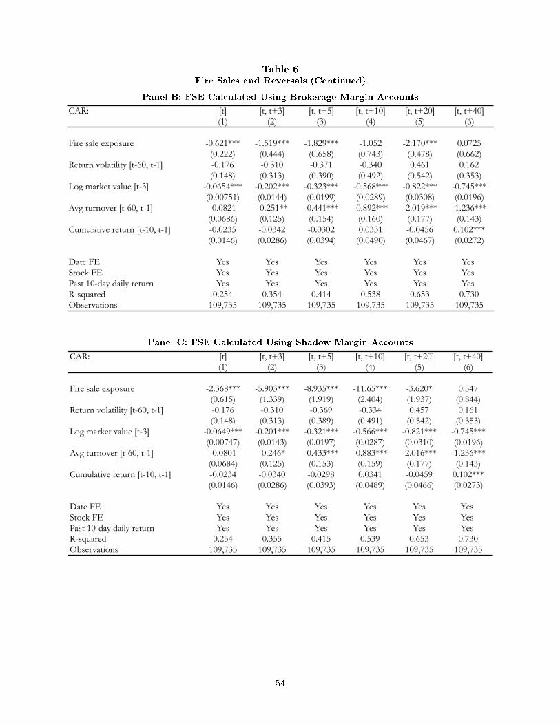
Table 6Fire Sales and Reversals (Continued)

Panel B: FSE Calculated Using Brokerage Margin Accounts

Full

CAR: [t] [t, t+3] [t, t+5] [t, t+10] [t, t+20] [t, t+40](1) (2) (3) (4) (5) (6)

Fire sale exposure -1.422*** -3.529*** -5.089*** -5.924*** -2.827*** 0.290(0.312) (0.594) (0.910) (1.264) (0.924) (0.570)

Return volatility [t-60, t-1] -0.172 -0.300 -0.356 -0.319 0.466 0.161(0.148) (0.313) (0.389) (0.491) (0.540) (0.353)

Log market value [t-3] -0.0652*** -0.201*** -0.322*** -0.568*** -0.822*** -0.745***(0.00749) (0.0144) (0.0198) (0.0288) (0.0308) (0.0196)

Avg turnover [t-60, t-1] -0.0809 -0.248* -0.436*** -0.888*** -2.017*** -1.236***(0.0685) (0.125) (0.154) (0.159) (0.177) (0.143)

Cumulative return [t-10, t-1] -0.0230 -0.0330 -0.0284 0.0356 -0.0450 0.102***(0.0146) (0.0285) (0.0393) (0.0489) (0.0465) (0.0271)

Date FE Yes Yes Yes Yes Yes Yes Stock FE Yes Yes Yes Yes Yes Yes Past 10-day daily return Yes Yes Yes Yes Yes Yes R-squared 0.254 0.354 0.415 0.538 0.653 0.730Observations 109,735 109,735 109,735 109,735 109,735 109,735

Brokerage

CAR: [t] [t, t+3] [t, t+5] [t, t+10] [t, t+20] [t, t+40](1) (2) (3) (4) (5) (6)

Fire sale exposure -0.621*** -1.519*** -1.829*** -1.052 -2.170*** 0.0725(0.222) (0.444) (0.658) (0.743) (0.478) (0.662)

Return volatility [t-60, t-1] -0.176 -0.310 -0.371 -0.340 0.461 0.162(0.148) (0.313) (0.390) (0.492) (0.542) (0.353)

Log market value [t-3] -0.0654*** -0.202*** -0.323*** -0.568*** -0.822*** -0.745***(0.00751) (0.0144) (0.0199) (0.0289) (0.0308) (0.0196)

Avg turnover [t-60, t-1] -0.0821 -0.251** -0.441*** -0.892*** -2.019*** -1.236***(0.0686) (0.125) (0.154) (0.160) (0.177) (0.143)

Cumulative return [t-10, t-1] -0.0235 -0.0342 -0.0302 0.0331 -0.0456 0.102***(0.0146) (0.0286) (0.0394) (0.0490) (0.0467) (0.0272)

Date FE Yes Yes Yes Yes Yes Yes Stock FE Yes Yes Yes Yes Yes Yes Past 10-day daily return Yes Yes Yes Yes Yes Yes R-squared 0.254 0.354 0.414 0.538 0.653 0.730Observations 109,735 109,735 109,735 109,735 109,735 109,735

Panel C: FSE Calculated Using Shadow Margin AccountsShadow

CAR: [t] [t, t+3] [t, t+5] [t, t+10] [t, t+20] [t, t+40](1) (2) (3) (4) (5) (6)

Fire sale exposure -2.368*** -5.903*** -8.935*** -11.65*** -3.620* 0.547(0.615) (1.339) (1.919) (2.404) (1.937) (0.844)

Return volatility [t-60, t-1] -0.176 -0.310 -0.369 -0.334 0.457 0.161(0.148) (0.313) (0.389) (0.491) (0.542) (0.353)

Log market value [t-3] -0.0649*** -0.201*** -0.321*** -0.566*** -0.821*** -0.745***(0.00747) (0.0143) (0.0197) (0.0287) (0.0310) (0.0196)

Avg turnover [t-60, t-1] -0.0801 -0.246* -0.433*** -0.883*** -2.016*** -1.236***(0.0684) (0.125) (0.153) (0.159) (0.177) (0.143)

Cumulative return [t-10, t-1] -0.0234 -0.0340 -0.0298 0.0341 -0.0459 0.102***(0.0146) (0.0286) (0.0393) (0.0489) (0.0466) (0.0273)

Date FE Yes Yes Yes Yes Yes Yes Stock FE Yes Yes Yes Yes Yes Yes Past 10-day daily return Yes Yes Yes Yes Yes Yes R-squared 0.254 0.355 0.415 0.539 0.653 0.730Observations 109,735 109,735 109,735 109,735 109,735 109,735

Full, Lambda weighted

CAR: [t] [t, t+3] [t, t+5] [t, t+10] [t, t+20] [t, t+40](1) (2) (3) (4) (5) (6)

Fire sale exposure -10.28*** -26.97*** -39.41*** -44.49*** -19.52*** 1.414(2.555) (5.247) (7.709) (10.41) (6.799) (4.030)

Return volatility [t-60, t-1] -0.170 -0.296 -0.349 -0.312 0.468 0.161(0.148) (0.312) (0.389) (0.490) (0.539) (0.353)

Log market value [t-3] -0.0652*** -0.201*** -0.322*** -0.568*** -0.822*** -0.745***(0.00749) (0.0144) (0.0198) (0.0288) (0.0308) (0.0196)

Avg turnover [t-60, t-1] -0.0808 -0.248* -0.436*** -0.887*** -2.017*** -1.236***(0.0685) (0.125) (0.154) (0.159) (0.177) (0.143)

Cumulative return [t-10, t-1] -0.0229 -0.0327 -0.0278 0.0362 -0.0449 0.102***(0.0146) (0.0285) (0.0392) (0.0489) (0.0464) (0.0272)

Date FE Yes Yes Yes Yes Yes Yes Stock FE Yes Yes Yes Yes Yes Yes Past 10-day daily return Yes Yes Yes Yes Yes Yes R-squared 0.254 0.355 0.415 0.539 0.653 0.730Observations 109,735 109,735 109,735 109,735 109,735 109,735

54

Table 7Regulatory Tightening

Regulatory tightening events occurred after hours on Friday May 22, 2015 and Friday June 12, 2015. Thistable shows the coe�cients λk from the regression de�ned in Table 2, estimated separately for the brokerage-and shadow-�nanced margin account samples on the �ve trading days immediately before and after theregulatory tightening events. Standard errors are allowed to be clustered at the stock level. ***, **, *correspond to statistical signi�cance at the 1%, 5%, and 10% levels, respectively.

Net sellingBroker Shadow Broker Shadow

(1) (2) (3) (4)

Proximity in (0/10 1/10) 0.00109 0.0342*** -0.00949*** 0.0242***(0.000917) (0.00949) (0.000865) (0.00821)

Proximity in [1/10 2/10) 0.00438*** 0.0193** 0.00254*** 0.0372***(0.000805) (0.00976) (0.000812) (0.00856)

Proximity in [2/10 3/10) 0.00856*** -0.00167 0.00901*** 0.0322***(0.000989) (0.00991) (0.00110) (0.00868)

Proximity in [3/10 4/10) 0.00846*** -0.0262*** 0.00278 0.0303***(0.00188) (0.00999) (0.00228) (0.00878)

Proximity in [4/10 5/10) 0.00622 -0.0457*** -0.0201*** 0.0322***(0.00442) (0.0101) (0.00702) (0.00892)

Proximity in [5/10 6/10) -0.0223** -0.0529*** 0.0143 0.0425***(0.00885) (0.0103) (0.0191) (0.00924)

Proximity in [6/10 7/10) -0.0394 -0.0580*** 0.0514 0.0560***(0.0293) (0.0106) (0.0460) (0.00974)

Proximity in [7/10 8/10) -0.0812** -0.0487*** -0.0463 0.0593***(0.0407) (0.0112) (0.0403) (0.0106)

Proximity in [8/10 9/10) -0.204*** -0.0551*** -0.108** 0.0939***(0.0578) (0.0118) (0.0483) (0.0118)

Proximity in [9/10 10/10) -0.301*** -0.0385*** -0.0434 0.0850***(0.0971) (0.0129) (0.0745) (0.0129)

Proximity >= 1 0.276 -0.0309** 0.262*** 0.0719***(0.199) (0.0120) (0.0965) (0.0105)

Proximity in (0/10 1/10) * after -0.00111 0.0163*** 0.00650*** 0.0396***(0.00101) (0.00368) (0.00101) (0.00253)

Proximity in [1/10 2/10) * after 0.00427*** 0.0139*** 0.0117*** 0.0237***(0.000934) (0.00225) (0.000866) (0.00165)

Proximity in [2/10 3/10) * after 0.00531*** 0.00587*** 0.0172*** 0.0200***(0.00123) (0.00194) (0.00110) (0.00158)

Proximity in [3/10 4/10) * after 0.00239 0.00937*** 0.0168*** 0.0254***(0.00258) (0.00210) (0.00230) (0.00178)

Proximity in [4/10 5/10) * after -0.00581 0.0211*** 0.0374*** 0.0404***(0.00772) (0.00282) (0.00747) (0.00235)

Proximity in [5/10 6/10) * after 0.0359** 0.0413*** 0.00791 0.0619***(0.0166) (0.00404) (0.0209) (0.00345)

Proximity in [6/10 7/10) * after -0.00138 0.0643*** -0.0298 0.109***(0.0533) (0.00571) (0.0503) (0.00483)

Proximity in [7/10 8/10) * after -0.0573 0.0933*** 0.0738 0.170***(0.0683) (0.00780) (0.0501) (0.00683)

Proximity in [8/10 9/10) * after -0.156 0.137*** 0.0736 0.170***(0.173) (0.0106) (0.0644) (0.00887)

Proximity in [9/10 10/10) * after 8.40e-05 0.156*** 0.203***(0.00678) (0.0136) (0.0113)

Proximity >= 1 * after 0.110*** 0.184***(0.00769) (0.00640)

Stock FE Yes Yes Yes YesR-squared 0.181 0.186 0.171 0.177Observations 53,107,983 51,622,691 59,177,319 57,717,993

May 22 event June 12 event

55

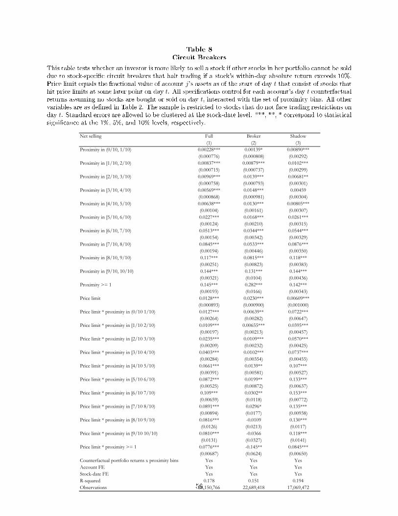
Table 8Circuit Breakers

This table tests whether an investor is more likely to sell a stock if other stocks in her portfolio cannot be solddue to stock-speci�c circuit breakers that halt trading if a stock's within-day absolute return exceeds 10%.Price limit equals the fractional value of account j's assets as of the start of day t that consist of stocks thathit price limits at some later point on day t. All speci�cations control for each account's day t counterfactualreturns assuming no stocks are bought or sold on day t, interacted with the set of proximity bins. All othervariables are as de�ned in Table 2. The sample is restricted to stocks that do not face trading restrictions onday t. Standard errors are allowed to be clustered at the stock-date level. ***, **, * correspond to statisticalsigni�cance at the 1%, 5%, and 10% levels, respectively.

Net selling Full Broker Shadow(1) (2) (3)

Proximity in (0/10, 1/10) 0.00228*** 0.00139* 0.00890***(0.000776) (0.000808) (0.00292)

Proximity in [1/10, 2/10) 0.00837*** 0.00879*** 0.0102***(0.000715) (0.000737) (0.00299)

Proximity in [2/10, 3/10) 0.00969*** 0.0139*** 0.00681**(0.000758) (0.000793) (0.00301)

Proximity in [3/10, 4/10) 0.00569*** 0.0148*** 0.00459(0.000868) (0.000981) (0.00304)

Proximity in [4/10, 5/10) 0.00638*** 0.0130*** 0.00805***(0.00104) (0.00161) (0.00307)

Proximity in [5/10, 6/10) 0.0227*** 0.0168*** 0.0261***(0.00124) (0.00210) (0.00315)

Proximity in [6/10, 7/10) 0.0513*** 0.0344*** 0.0544***(0.00154) (0.00342) (0.00329)

Proximity in [7/10, 8/10) 0.0845*** 0.0533*** 0.0876***(0.00194) (0.00446) (0.00350)

Proximity in [8/10, 9/10) 0.117*** 0.0815*** 0.118***(0.00251) (0.00823) (0.00383)

Proximity in [9/10, 10/10) 0.144*** 0.131*** 0.144***(0.00321) (0.0104) (0.00436)

Proximity >= 1 0.145*** 0.282*** 0.142***(0.00193) (0.0166) (0.00343)

Price limit 0.0128*** 0.0230*** 0.00609***(0.000893) (0.000900) (0.001000)

Price limit * proximity in (0/10 1/10) 0.0127*** 0.00639** 0.0722***(0.00264) (0.00282) (0.00647)

Price limit * proximity in [1/10 2/10) 0.0109*** 0.00655*** 0.0395***(0.00197) (0.00213) (0.00457)

Price limit * proximity in [2/10 3/10) 0.0235*** 0.0109*** 0.0570***(0.00209) (0.00232) (0.00425)

Price limit * proximity in [3/10 4/10) 0.0403*** 0.0102*** 0.0737***(0.00284) (0.00354) (0.00455)

Price limit * proximity in [4/10 5/10) 0.0661*** 0.0139** 0.107***(0.00391) (0.00581) (0.00527)

Price limit * proximity in [5/10 6/10) 0.0872*** 0.0199** 0.133***(0.00525) (0.00872) (0.00637)

Price limit * proximity in [6/10 7/10) 0.109*** 0.0302** 0.153***(0.00659) (0.0118) (0.00772)

Price limit * proximity in [7/10 8/10) 0.0891*** 0.0296* 0.135***(0.00894) (0.0177) (0.00938)

Price limit * proximity in [8/10 9/10) 0.0816*** -0.0109 0.130***(0.0126) (0.0213) (0.0117)

Price limit * proximity in [9/10 10/10) 0.0810*** -0.0366 0.118***(0.0131) (0.0327) (0.0141)

Price limit * proximity >= 1 0.0776*** -0.145** 0.0845***(0.00687) (0.0624) (0.00650)

Counterfactual portfolio returns x proximity bins Yes Yes YesAccount FE Yes Yes YesStock-date FE Yes Yes YesR-squared 0.178 0.151 0.194Observations 28,150,766 22,689,418 17,069,47256

A Data Appendix

The shadow-�nanced margin account data is organized in a umbella-style structure. There are155,531 child accounts, each of which is connected to a few mother accounts maintained by thesame trading platform. For each account, we observe the initial lending ratio of the borrower,de�ned as the amount of borrowing divided by the investor's margin deposit (equity). We alsoobserve the minimum coverage ratio, the ratio of remaining assets / initial debt, that will trigger amargin call.

A.1 Data Filter

We adopt the following procedure to clean our data.

1. We eliminate accounts with invalid initial margin and maintenance margin information. Werequire the initial lending ratio to be less than 100. There are some accounts with extremelyhigh initial lending ratios. They are usually used as a bonus to investors with much lowerlending ratios and typically carry very little assets. On the other hand, we require the minimum

coverage ratio to be above 1, i.e, investors will receive the margin calls before outstanding debtexceeds the current asset wealth. Agent accounts with margin information not within theseranges might be maintained by non-margin accounts.

2. We require the �rst record in the margin accounts to be a cash �ow from the mother account,before the account starts any trading activities. These cash �ows usually occur right after theaccount opens, and includes the loans from the lenders together with the deposited marginsfrom the borrowers. We eliminate observations from accounts that either never have any cash�ows from mother accounts, or the �rst cash �ows are from the child accounts to the motheraccounts.

3. We also compare the size of initial cash �ows and the initial debt information provided bythe trading platform, and further eliminate observations from accounts for which the size ofthe initial cash �ow deviates signi�cantly from the initial debt reported by the online tradingsystem.

A.2 Construction of daily debt level

The shadow accounts data includes all variables in the brokerage account data, except for theend-of-day leverage numbers. Instead, the trading platform provides detailed information on theinitial debt, subsequent cash �ows between the mother account (controlled by the lender) and childaccounts (controlled by the borrowers), and all trades by the child accounts. We can thus manuallycalculate the end-of-day asset and debt value for each child account.

To construct daily outstanding debt for each margin child account in our dataset, we rely onthe cash �ow information between the mother and child accounts, as well as transaction remarks,both provided by the trading platform. For about two-thirds of the accounts, the platform providesdetailed remarks for each cash �ow (whether it is an issued loan or loan repayment), which helps uscalculate the exact daily outstanding debt levels. For the remaining accounts without transactionremarks, we assume that cash �ows to (from) the mother account exceeding 20% of the margin debtin the child account re�ects a payment of existing debt (additional borrowing). This 20% cuto�rule is suggested by the practitioners in the trading platform.

57

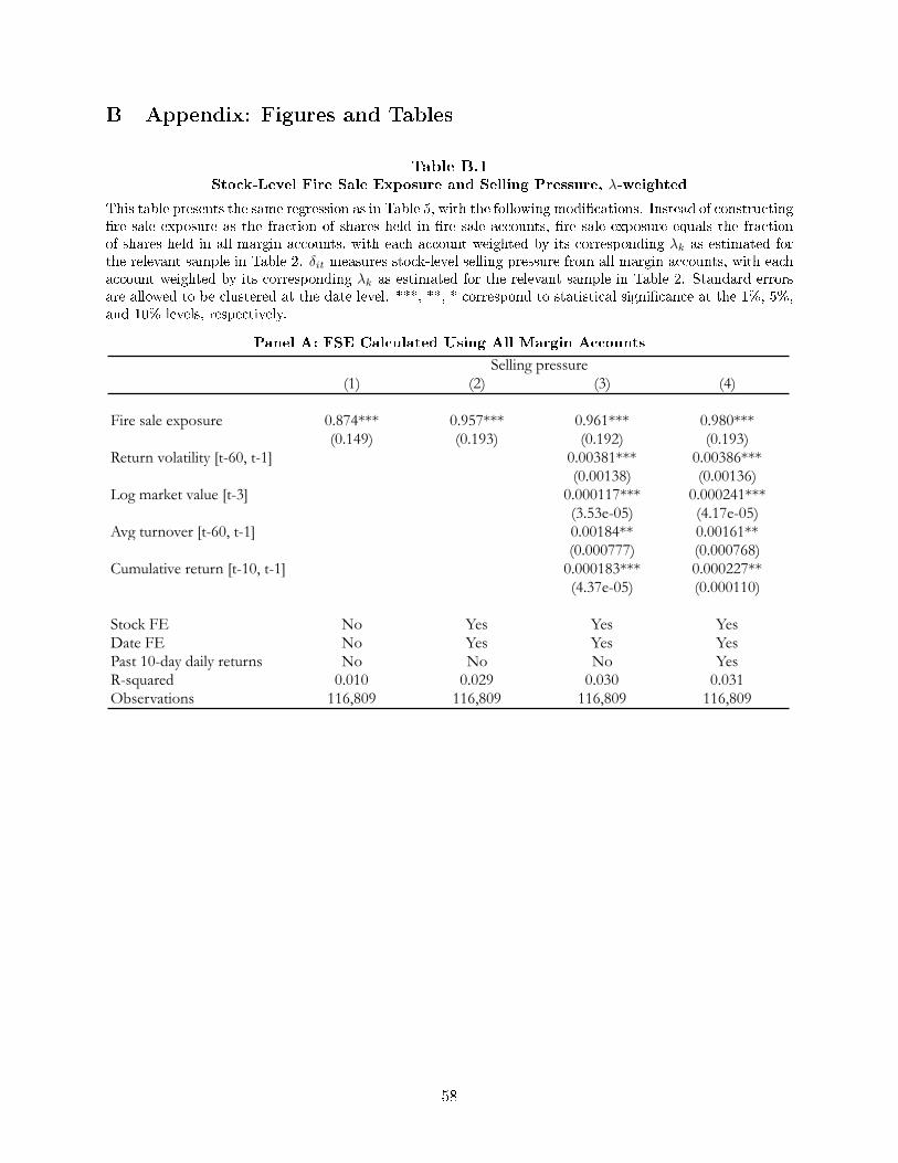
B Appendix: Figures and Tables

Table B.1Stock-Level Fire Sale Exposure and Selling Pressure, λ-weighted

This table presents the same regression as in Table 5, with the following modi�cations. Instead of constructing�re sale exposure as the fraction of shares held in �re sale accounts, �re sale exposure equals the fractionof shares held in all margin accounts, with each account weighted by its corresponding λk as estimated forthe relevant sample in Table 2. δit measures stock-level selling pressure from all margin accounts, with eachaccount weighted by its corresponding λk as estimated for the relevant sample in Table 2. Standard errorsare allowed to be clustered at the date level. ***, **, * correspond to statistical signi�cance at the 1%, 5%,and 10% levels, respectively.

Panel A: FSE Calculated Using All Margin Accounts

Shadow

(1) (2) (3) (4)

Fire sale exposure 0.113*** 0.125*** 0.124*** 0.124***(0.0341) (0.0417) (0.0418) (0.0418)

Return volatility [t-60, t-1] -0.000109 -3.68e-05(0.000167) (0.000163)

Log market value [t-3] 2.00e-05** 8.97e-06(8.66e-06) (7.18e-06)

Avg turnover [t-60, t-1] -0.000108 -9.08e-05(0.000142) (0.000147)

Cumulative return [t-10, t-1] -1.91e-05*** 3.15e-05**(7.14e-06) (1.40e-05)

Stock FE No Yes Yes YesDate FE No Yes Yes YesPast 10-day daily returns No No No YesR-squared 0.144 0.189 0.189 0.191Observations 116,809 116,809 116,809 116,809

Baseline, Lambda weighted

(1) (2) (3) (4)

Fire sale exposure 0.874*** 0.957*** 0.961*** 0.980***(0.149) (0.193) (0.192) (0.193)

Return volatility [t-60, t-1] 0.00381*** 0.00386***(0.00138) (0.00136)

Log market value [t-3] 0.000117*** 0.000241***(3.53e-05) (4.17e-05)

Avg turnover [t-60, t-1] 0.00184** 0.00161**(0.000777) (0.000768)

Cumulative return [t-10, t-1] 0.000183*** 0.000227**(4.37e-05) (0.000110)

Stock FE No Yes Yes YesDate FE No Yes Yes YesPast 10-day daily returns No No No YesR-squared 0.010 0.029 0.030 0.031Observations 116,809 116,809 116,809 116,809

Selling pressure

Selling pressure

58

Table B.1Stock-Level Fire Sale Exposure and Selling Pressure, λ-weighted (Continued)

Panel B: FSE Calculated Using Brokerage Margin AccountsBroker, Lambda weighted

(1) (2) (3) (4)

Fire sale exposure 1.351*** 1.466*** 1.479*** 1.510***(0.218) (0.291) (0.294) (0.299)

Return volatility [t-60, t-1] 0.00362*** 0.00359***(0.00133) (0.00127)

Log market value [t-3] -1.15e-05 0.000154***(3.27e-05) (3.75e-05)

Avg turnover [t-60, t-1] 0.00155** 0.00130*(0.000712) (0.000709)

Cumulative return [t-10, t-1] 0.000220*** 0.000249**(4.01e-05) (0.000105)

Stock FE No Yes Yes YesDate FE No Yes Yes YesPast 10-day daily returns No No No YesR-squared 0.006 0.018 0.020 0.022Observations 116,809 116,809 116,809 116,809

Shadow, Lambda weighted

(1) (2) (3) (4)

Fire sale exposure 0.714*** 0.953*** 0.942*** 0.934***(0.177) (0.220) (0.222) (0.222)

Return volatility [t-60, t-1] 0.000169 0.000240(0.000486) (0.000477)

Log market value [t-3] 0.000126*** 8.55e-05***(1.77e-05) (1.70e-05)

Avg turnover [t-60, t-1] 0.000287 0.000326(0.000300) (0.000302)

Cumulative return [t-10, t-1] -3.65e-05** -2.78e-05(1.41e-05) (3.71e-05)

Stock FE No Yes Yes YesDate FE No Yes Yes YesPast 10-day daily returns No No No YesR-squared 0.028 0.073 0.074 0.076Observations 116,809 116,809 116,809 116,809

Selling pressure

Selling pressure

Panel C: FSE Calculated Using Shadow Margin Accounts

Broker, Lambda weighted

(1) (2) (3) (4)

Fire sale exposure 1.351*** 1.466*** 1.479*** 1.510***(0.218) (0.291) (0.294) (0.299)

Return volatility [t-60, t-1] 0.00362*** 0.00359***(0.00133) (0.00127)

Log market value [t-3] -1.15e-05 0.000154***(3.27e-05) (3.75e-05)

Avg turnover [t-60, t-1] 0.00155** 0.00130*(0.000712) (0.000709)

Cumulative return [t-10, t-1] 0.000220*** 0.000249**(4.01e-05) (0.000105)

Stock FE No Yes Yes YesDate FE No Yes Yes YesPast 10-day daily returns No No No YesR-squared 0.006 0.018 0.020 0.022Observations 116,809 116,809 116,809 116,809

Shadow, Lambda weighted

(1) (2) (3) (4)

Fire sale exposure 0.714*** 0.953*** 0.942*** 0.934***(0.177) (0.220) (0.222) (0.222)

Return volatility [t-60, t-1] 0.000169 0.000240(0.000486) (0.000477)

Log market value [t-3] 0.000126*** 8.55e-05***(1.77e-05) (1.70e-05)

Avg turnover [t-60, t-1] 0.000287 0.000326(0.000300) (0.000302)

Cumulative return [t-10, t-1] -3.65e-05** -2.78e-05(1.41e-05) (3.71e-05)

Stock FE No Yes Yes YesDate FE No Yes Yes YesPast 10-day daily returns No No No YesR-squared 0.028 0.073 0.074 0.076Observations 116,809 116,809 116,809 116,809

Selling pressure

Selling pressure

59

Table B.2Fire Sales and Reversals, λ-weighted

This table presents the same regression as in Table 6, with the following modi�cations. Instead of constructing�re sale exposure as the fraction of shares held in �re sale accounts, �re sale exposure equals the fractionof shares held in all margin accounts, with each account weighted by its corresponding λk as estimated forthe relevant sample in Table 2. Standard errors are allowed to be clustered at the date level. ***, **, *correspond to statistical signi�cance at the 1%, 5%, and 10% levels, respectively.

Panel A: FSE Calculated Using All Margin Accounts

Shadow

CAR: [t] [t, t+3] [t, t+5] [t, t+10] [t, t+20] [t, t+40](1) (2) (3) (4) (5) (6)

Fire sale exposure -2.368*** -5.903*** -8.935*** -11.65*** -3.620* 0.547(0.615) (1.339) (1.919) (2.404) (1.937) (0.844)

Return volatility [t-60, t-1] -0.176 -0.310 -0.369 -0.334 0.457 0.161(0.148) (0.313) (0.389) (0.491) (0.542) (0.353)

Log market value [t-3] -0.0649*** -0.201*** -0.321*** -0.566*** -0.821*** -0.745***(0.00747) (0.0143) (0.0197) (0.0287) (0.0310) (0.0196)

Avg turnover [t-60, t-1] -0.0801 -0.246* -0.433*** -0.883*** -2.016*** -1.236***(0.0684) (0.125) (0.153) (0.159) (0.177) (0.143)

Cumulative return [t-10, t-1] -0.0234 -0.0340 -0.0298 0.0341 -0.0459 0.102***(0.0146) (0.0286) (0.0393) (0.0489) (0.0466) (0.0273)

Date FE Yes Yes Yes Yes Yes Yes Stock FE Yes Yes Yes Yes Yes Yes Past 10-day daily return Yes Yes Yes Yes Yes Yes R-squared 0.254 0.355 0.415 0.539 0.653 0.730Observations 109,735 109,735 109,735 109,735 109,735 109,735

Full, Lambda weighted

CAR: [t] [t, t+3] [t, t+5] [t, t+10] [t, t+20] [t, t+40](1) (2) (3) (4) (5) (6)

Fire sale exposure -10.28*** -26.97*** -39.41*** -44.49*** -19.52*** 1.414(2.555) (5.247) (7.709) (10.41) (6.799) (4.030)

Return volatility [t-60, t-1] -0.170 -0.296 -0.349 -0.312 0.468 0.161(0.148) (0.312) (0.389) (0.490) (0.539) (0.353)

Log market value [t-3] -0.0652*** -0.201*** -0.322*** -0.568*** -0.822*** -0.745***(0.00749) (0.0144) (0.0198) (0.0288) (0.0308) (0.0196)

Avg turnover [t-60, t-1] -0.0808 -0.248* -0.436*** -0.887*** -2.017*** -1.236***(0.0685) (0.125) (0.154) (0.159) (0.177) (0.143)

Cumulative return [t-10, t-1] -0.0229 -0.0327 -0.0278 0.0362 -0.0449 0.102***(0.0146) (0.0285) (0.0392) (0.0489) (0.0464) (0.0272)

Date FE Yes Yes Yes Yes Yes Yes Stock FE Yes Yes Yes Yes Yes Yes Past 10-day daily return Yes Yes Yes Yes Yes Yes R-squared 0.254 0.355 0.415 0.539 0.653 0.730Observations 109,735 109,735 109,735 109,735 109,735 109,735

60

Table B.2Fire Sales and Reversals, λ-weighted (Continued)

Panel B: FSE Calculated Using Brokerage Margin AccountsBrokerage, Lambda weighted

CAR: [t] [t, t+3] [t, t+5] [t, t+10] [t, t+20] [t, t+40](1) (2) (3) (4) (5) (6)

Fire sale exposure -7.332*** -21.71*** -28.25*** -19.31*** -25.29*** -2.584(2.257) (4.610) (5.337) (4.870) (6.224) (10.01)

Return volatility [t-60, t-1] -0.175 -0.306 -0.365 -0.336 0.464 0.163(0.148) (0.313) (0.390) (0.492) (0.541) (0.353)

Log market value [t-3] -0.0654*** -0.202*** -0.323*** -0.568*** -0.822*** -0.745***(0.00751) (0.0144) (0.0199) (0.0289) (0.0307) (0.0196)

Avg turnover [t-60, t-1] -0.0822 -0.251** -0.441*** -0.893*** -2.020*** -1.236***(0.0686) (0.125) (0.154) (0.160) (0.177) (0.143)

Cumulative return [t-10, t-1] -0.0234 -0.0339 -0.0297 0.0335 -0.0453 0.103***(0.0146) (0.0286) (0.0394) (0.0490) (0.0466) (0.0271)

Date FE Yes Yes Yes Yes Yes Yes Stock FE Yes Yes Yes Yes Yes Yes Past 10-day daily return Yes Yes Yes Yes Yes Yes R-squared 0.254 0.354 0.414 0.538 0.653 0.730Observations 109,735 109,735 109,735 109,735 109,735 109,735

Shadow, Lambda weighted

CAR: [t] [t, t+3] [t, t+5] [t, t+10] [t, t+20] [t, t+40](1) (2) (3) (4) (5) (6)

Fire sale exposure -13.64*** -34.55*** -52.55*** -68.79*** -23.97** -0.0958(3.616) (7.846) (11.06) (14.46) (10.82) (4.518)

Return volatility [t-60, t-1] -0.176 -0.310 -0.370 -0.335 0.457 0.162(0.148) (0.313) (0.389) (0.491) (0.542) (0.354)

Log market value [t-3] -0.0649*** -0.200*** -0.321*** -0.566*** -0.821*** -0.745***(0.00747) (0.0143) (0.0197) (0.0286) (0.0310) (0.0196)

Avg turnover [t-60, t-1] -0.0802 -0.246* -0.434*** -0.883*** -2.016*** -1.236***(0.0684) (0.125) (0.154) (0.159) (0.177) (0.143)

Cumulative return [t-10, t-1] -0.0234 -0.0341 -0.0299 0.0340 -0.0459 0.103***(0.0146) (0.0286) (0.0393) (0.0489) (0.0466) (0.0273)

Date FE Yes Yes Yes Yes Yes Yes Stock FE Yes Yes Yes Yes Yes Yes Past 10-day daily return Yes Yes Yes Yes Yes Yes R-squared 0.254 0.355 0.415 0.539 0.653 0.730Observations 109,735 109,735 109,735 109,735 109,735 109,735

Panel C: FSE Calculated Using Shadow Margin Accounts

Brokerage, Lambda weighted

CAR: [t] [t, t+3] [t, t+5] [t, t+10] [t, t+20] [t, t+40](1) (2) (3) (4) (5) (6)

Fire sale exposure -7.332*** -21.71*** -28.25*** -19.31*** -25.29*** -2.584(2.257) (4.610) (5.337) (4.870) (6.224) (10.01)

Return volatility [t-60, t-1] -0.175 -0.306 -0.365 -0.336 0.464 0.163(0.148) (0.313) (0.390) (0.492) (0.541) (0.353)

Log market value [t-3] -0.0654*** -0.202*** -0.323*** -0.568*** -0.822*** -0.745***(0.00751) (0.0144) (0.0199) (0.0289) (0.0307) (0.0196)

Avg turnover [t-60, t-1] -0.0822 -0.251** -0.441*** -0.893*** -2.020*** -1.236***(0.0686) (0.125) (0.154) (0.160) (0.177) (0.143)

Cumulative return [t-10, t-1] -0.0234 -0.0339 -0.0297 0.0335 -0.0453 0.103***(0.0146) (0.0286) (0.0394) (0.0490) (0.0466) (0.0271)

Date FE Yes Yes Yes Yes Yes Yes Stock FE Yes Yes Yes Yes Yes Yes Past 10-day daily return Yes Yes Yes Yes Yes Yes R-squared 0.254 0.354 0.414 0.538 0.653 0.730Observations 109,735 109,735 109,735 109,735 109,735 109,735

Shadow, Lambda weighted

CAR: [t] [t, t+3] [t, t+5] [t, t+10] [t, t+20] [t, t+40](1) (2) (3) (4) (5) (6)

Fire sale exposure -13.64*** -34.55*** -52.55*** -68.79*** -23.97** -0.0958(3.616) (7.846) (11.06) (14.46) (10.82) (4.518)

Return volatility [t-60, t-1] -0.176 -0.310 -0.370 -0.335 0.457 0.162(0.148) (0.313) (0.389) (0.491) (0.542) (0.354)

Log market value [t-3] -0.0649*** -0.200*** -0.321*** -0.566*** -0.821*** -0.745***(0.00747) (0.0143) (0.0197) (0.0286) (0.0310) (0.0196)

Avg turnover [t-60, t-1] -0.0802 -0.246* -0.434*** -0.883*** -2.016*** -1.236***(0.0684) (0.125) (0.154) (0.159) (0.177) (0.143)

Cumulative return [t-10, t-1] -0.0234 -0.0341 -0.0299 0.0340 -0.0459 0.103***(0.0146) (0.0286) (0.0393) (0.0489) (0.0466) (0.0273)

Date FE Yes Yes Yes Yes Yes Yes Stock FE Yes Yes Yes Yes Yes Yes Past 10-day daily return Yes Yes Yes Yes Yes Yes R-squared 0.254 0.355 0.415 0.539 0.653 0.730Observations 109,735 109,735 109,735 109,735 109,735 109,735

61

Table B.3Fire Sales and Reversals, Excluding Imputed Prices

This table presents the same regressions as in Table 6, but exclude stocks that ever experienced a full dayof suspended trading during the event period [t, t + 40]. In our baseline analysis, we impute stock pricesand returns for trading days in which a particularly stock did not trade. The imputation procedure usesinformation on the most recent traded prices before and after the trading suspension. Standard errors areallowed to be clustered at the date level. ***, **, * correspond to statistical signi�cance at the 1%, 5%, and10% levels, respectively.

Panel A: FSE Calculated Using All Margin AccountsFull, no imputation

CAR: [t] [t, t+3] [t, t+5] [t, t+10] [t, t+20] [t, t+40](1) (2) (3) (4) (5) (6)

Fire sale exposure -1.528*** -3.738*** -5.476*** -6.319*** -2.851** -1.318*(0.506) (1.019) (1.534) (1.783) (1.248) (0.744)

Return volatility [t-60, t-1] -0.175 -0.398 -0.427 -0.180 0.615 0.998**(0.179) (0.362) (0.450) (0.589) (0.631) (0.418)

Log market value [t-3] -0.0617*** -0.189*** -0.304*** -0.546*** -0.814*** -0.716***(0.00879) (0.0162) (0.0241) (0.0389) (0.0387) (0.0203)

Avg turnover [t-60, t-1] -0.0950 -0.288** -0.549*** -1.100*** -2.202*** -1.710***(0.0688) (0.119) (0.142) (0.162) (0.185) (0.154)

Cumulative return [t-10, t-1] -0.0259 -0.0273 0.00629 0.104* -0.00111 0.0917***(0.0163) (0.0330) (0.0453) (0.0546) (0.0480) (0.0325)

Date FE Yes Yes Yes Yes Yes Yes Stock FE Yes Yes Yes Yes Yes Yes Past 10-day daily return Yes Yes Yes Yes Yes Yes R-squared 0.250 0.348 0.404 0.513 0.637 0.734Observations 68,123 68,123 68,123 68,123 68,123 68,123

Brokerage, no imputation

CAR: [t] [t, t+3] [t, t+5] [t, t+10] [t, t+20] [t, t+40](1) (2) (3) (4) (5) (6)

Fire sale exposure -0.691 -1.270 -0.284 0.815 -1.026 -3.379***(0.516) (1.026) (1.526) (1.581) (0.978) (0.913)

Return volatility [t-60, t-1] -0.181 -0.413 -0.454 -0.214 0.603 1.002**(0.179) (0.363) (0.452) (0.591) (0.634) (0.419)

Log market value [t-3] -0.0620*** -0.189*** -0.305*** -0.547*** -0.814*** -0.716***(0.00883) (0.0163) (0.0243) (0.0390) (0.0386) (0.0203)

Avg turnover [t-60, t-1] -0.0960 -0.290** -0.553*** -1.104*** -2.204*** -1.711***(0.0689) (0.119) (0.142) (0.163) (0.185) (0.154)

Cumulative return [t-10, t-1] -0.0262 -0.0283 0.00437 0.102* -0.00185 0.0922***(0.0162) (0.0331) (0.0453) (0.0546) (0.0482) (0.0325)

Date FE Yes Yes Yes Yes Yes Yes Stock FE Yes Yes Yes Yes Yes Yes Past 10-day daily return Yes Yes Yes Yes Yes Yes R-squared 0.250 0.347 0.403 0.513 0.637 0.734Observations 68,123 68,123 68,123 68,123 68,123 68,123

62

Table B.3Fire Sales and Reversals, Excluding Imputed Prices (Continued)

Panel B: FSE Calculated Using Brokerage Margin Accounts

Full, no imputation

CAR: [t] [t, t+3] [t, t+5] [t, t+10] [t, t+20] [t, t+40](1) (2) (3) (4) (5) (6)

Fire sale exposure -1.528*** -3.738*** -5.476*** -6.319*** -2.851** -1.318*(0.506) (1.019) (1.534) (1.783) (1.248) (0.744)

Return volatility [t-60, t-1] -0.175 -0.398 -0.427 -0.180 0.615 0.998**(0.179) (0.362) (0.450) (0.589) (0.631) (0.418)

Log market value [t-3] -0.0617*** -0.189*** -0.304*** -0.546*** -0.814*** -0.716***(0.00879) (0.0162) (0.0241) (0.0389) (0.0387) (0.0203)

Avg turnover [t-60, t-1] -0.0950 -0.288** -0.549*** -1.100*** -2.202*** -1.710***(0.0688) (0.119) (0.142) (0.162) (0.185) (0.154)

Cumulative return [t-10, t-1] -0.0259 -0.0273 0.00629 0.104* -0.00111 0.0917***(0.0163) (0.0330) (0.0453) (0.0546) (0.0480) (0.0325)

Date FE Yes Yes Yes Yes Yes Yes Stock FE Yes Yes Yes Yes Yes Yes Past 10-day daily return Yes Yes Yes Yes Yes Yes R-squared 0.250 0.348 0.404 0.513 0.637 0.734Observations 68,123 68,123 68,123 68,123 68,123 68,123

Brokerage, no imputation

CAR: [t] [t, t+3] [t, t+5] [t, t+10] [t, t+20] [t, t+40](1) (2) (3) (4) (5) (6)

Fire sale exposure -0.691 -1.270 -0.284 0.815 -1.026 -3.379***(0.516) (1.026) (1.526) (1.581) (0.978) (0.913)

Return volatility [t-60, t-1] -0.181 -0.413 -0.454 -0.214 0.603 1.002**(0.179) (0.363) (0.452) (0.591) (0.634) (0.419)

Log market value [t-3] -0.0620*** -0.189*** -0.305*** -0.547*** -0.814*** -0.716***(0.00883) (0.0163) (0.0243) (0.0390) (0.0386) (0.0203)

Avg turnover [t-60, t-1] -0.0960 -0.290** -0.553*** -1.104*** -2.204*** -1.711***(0.0689) (0.119) (0.142) (0.163) (0.185) (0.154)

Cumulative return [t-10, t-1] -0.0262 -0.0283 0.00437 0.102* -0.00185 0.0922***(0.0162) (0.0331) (0.0453) (0.0546) (0.0482) (0.0325)

Date FE Yes Yes Yes Yes Yes Yes Stock FE Yes Yes Yes Yes Yes Yes Past 10-day daily return Yes Yes Yes Yes Yes Yes R-squared 0.250 0.347 0.403 0.513 0.637 0.734Observations 68,123 68,123 68,123 68,123 68,123 68,123

Panel C: FSE Calculated Using Shadow Margin AccountsShadow, no imputation

CAR: [t] [t, t+3] [t, t+5] [t, t+10] [t, t+20] [t, t+40](1) (2) (3) (4) (5) (6)

Fire sale exposure -2.003*** -5.141*** -8.422*** -10.37*** -3.889* -0.153(0.696) (1.621) (2.461) (2.880) (2.017) (1.005)

Return volatility [t-60, t-1] -0.179 -0.407 -0.438 -0.191 0.608 0.992**(0.179) (0.363) (0.450) (0.590) (0.632) (0.420)

Log market value [t-3] -0.0615*** -0.188*** -0.303*** -0.545*** -0.813*** -0.716***(0.00878) (0.0161) (0.0239) (0.0387) (0.0388) (0.0203)

Avg turnover [t-60, t-1] -0.0946 -0.286** -0.547*** -1.097*** -2.202*** -1.711***(0.0687) (0.119) (0.142) (0.163) (0.185) (0.154)

Cumulative return [t-10, t-1] -0.0263 -0.0283 0.00492 0.103* -0.00186 0.0912***(0.0163) (0.0332) (0.0454) (0.0546) (0.0481) (0.0326)

Date FE Yes Yes Yes Yes Yes Yes Stock FE Yes Yes Yes Yes Yes Yes Past 10-day daily return Yes Yes Yes Yes Yes Yes R-squared 0.250 0.348 0.404 0.514 0.637 0.734Observations 68,123 68,123 68,123 68,123 68,123 68,123

63