Lecture 17 parametric curves and surfacescommunity.wvu.edu/~bpbettig/MAE455/Lecture_17... · MAE...
18
MAE 455 Computer-Aided Design and Drafting Parametric Representation of Curves and Surfaces How does the computer compute curves and surfaces?
Transcript of Lecture 17 parametric curves and surfacescommunity.wvu.edu/~bpbettig/MAE455/Lecture_17... · MAE...

MAE 455 Computer-Aided Design and Drafting
Parametric Representation of Curves and Surfaces
How does the computer compute curves and surfaces?
MAE 455 Computer-Aided Design and Drafting 2
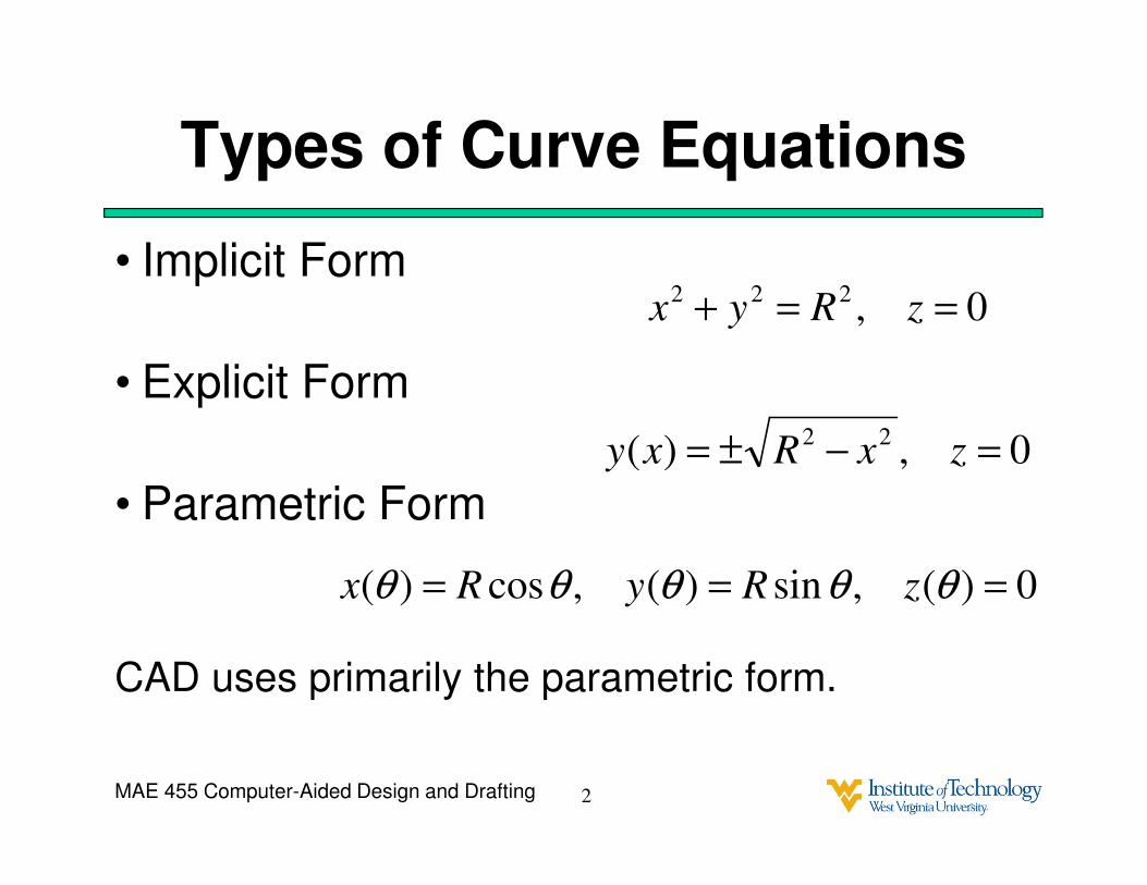
Types of Curve Equations
• Implicit Form
• Explicit Form
• Parametric Form
CAD uses primarily the parametric form.
0 ,222==+ zRyx
0 ,)( 22=−±= zxRxy
0)( ,sin)( ,cos)( === θθθθθ zRyRx
MAE 455 Computer-Aided Design and Drafting 3
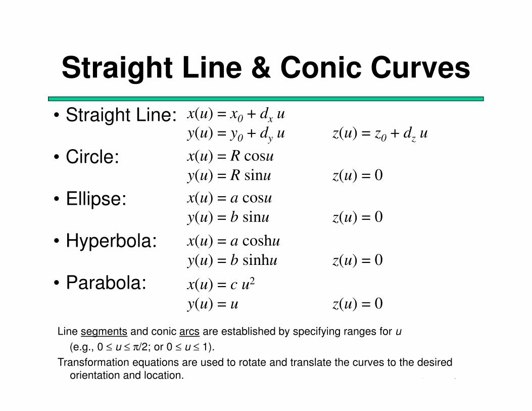
Straight Line & Conic Curves
• Straight Line:
• Circle:
• Ellipse:
• Hyperbola:
• Parabola:
x(u) = R cosu
y(u) = R sinu z(u) = 0
x(u) = a cosu
y(u) = b sinu z(u) = 0
x(u) = a coshu
y(u) = b sinhu z(u) = 0
x(u) = c u2
y(u) = u z(u) = 0
Line segments and conic arcs are established by specifying ranges for u
(e.g., 0 ≤ u ≤ π/2; or 0 ≤ u ≤ 1).
Transformation equations are used to rotate and translate the curves to the desired
orientation and location.
x(u) = x0 + dx u
y(u) = y0 + dy u z(u) = z0 + dz u
MAE 455 Computer-Aided Design and Drafting 4
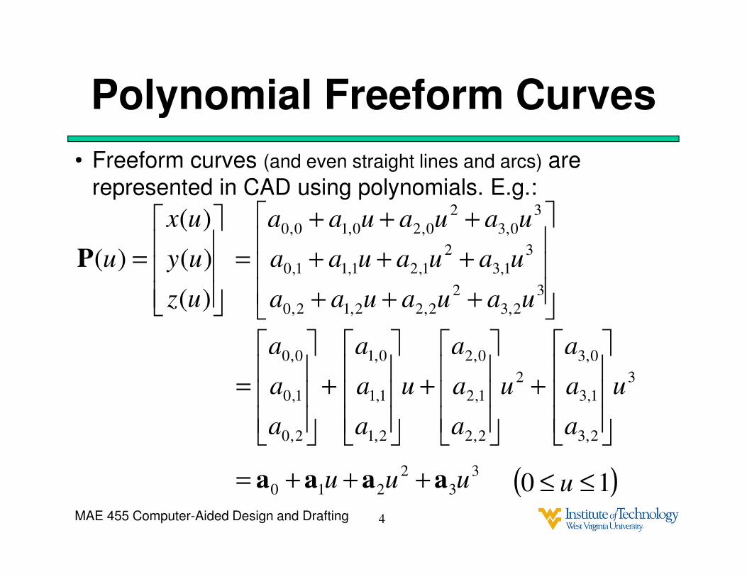
Polynomial Freeform Curves
• Freeform curves (and even straight lines and arcs) are
represented in CAD using polynomials. E.g.:
=
)(
)(
)(
)(
uz
uy
ux
uP
3
3
2
210 uuu aaaa +++=
+++
=
3
0,3
2
0,20,10,0 uauauaa3
1,3
2
1,21,11,0 uauauaa +++3
2,3
2
2,22,12,0 uauauaa +++
+
=
2,0
1,0
0,0
a
a
a
+
2
2,2
1,2
0,2
u
a
a
a
+
u
a
a
a
2,1
1,1
0,1
3
2,3
1,3
0,3
u
a
a
a
( )10 ≤≤ u

MAE 455 Computer-Aided Design and Drafting 5
B-Spline Curve
• The coefficients a0, a1, a2, a3 are hard for a designer to specify because the geometric affect is not intuitive.
• CAD software therefore uses “B-Spline” curves.• B-Spline curves are controlled using “control points” .
B-Spline curve with:
– Degree: 3
– Num. control points: 4
P0 (u = 0)
P3(u = 1)
P1 P2
“control points”
(“poles” in NX)
“control” polyline
MAE 455 Computer-Aided Design and Drafting 6
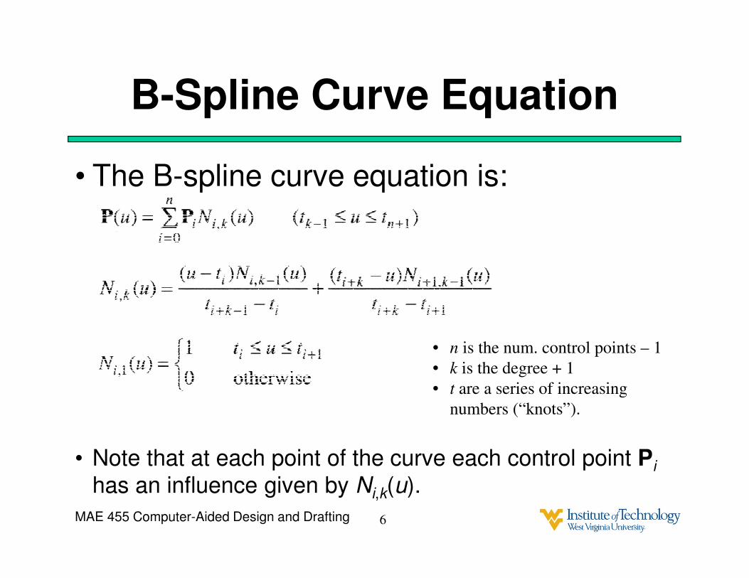
B-Spline Curve Equation
• The B-spline curve equation is:
• Note that at each point of the curve each control point Pi
has an influence given by Ni,k(u).
• n is the num. control points – 1
• k is the degree + 1
• t are a series of increasing
numbers (“knots”).

MAE 455 Computer-Aided Design and Drafting 7
B-Spline Curve Equation
Degree: 7
Num. control points: 8
• Using a smaller degree limits the influence of each control point.
Degree: 3
Num. control points: 8
N0,4
N1,4 N2,4N3,4 N4,4 N5,4 N6,4
N7,4
u
N0,8
N3,8
N6,8N5,8N1,8 N4,8
N2,8
N7,8
u
Blue triangles represent knots
MAE 455 Computer-Aided Design and Drafting
u = 0
u = tlast
u = 0
u = tlast
8
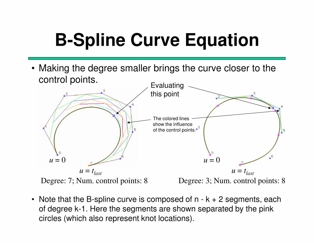
B-Spline Curve Equation
Degree: 7; Num. control points: 8
Evaluating
this point
• Note that the B-spline curve is composed of n - k + 2 segments, each of degree k-1. Here the segments are shown separated by the pink circles (which also represent knot locations).
• Making the degree smaller brings the curve closer to the
control points.
Degree: 3; Num. control points: 8
The colored lines
show the influence
of the control points.
MAE 455 Computer-Aided Design and Drafting 9
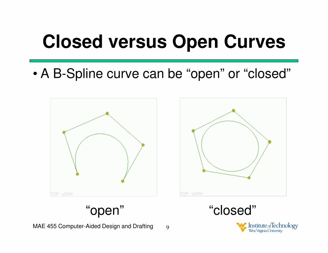
Closed versus Open Curves
• A B-Spline curve can be “open” or “closed”
“open” “closed”
MAE 455 Computer-Aided Design and Drafting 10
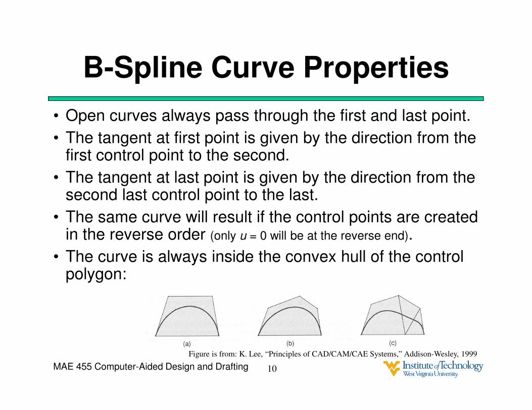
B-Spline Curve Properties
• Open curves always pass through the first and last point.
• The tangent at first point is given by the direction from the first control point to the second.
• The tangent at last point is given by the direction from the second last control point to the last.
• The same curve will result if the control points are created in the reverse order (only u = 0 will be at the reverse end).
• The curve is always inside the convex hull of the control polygon:
Figure is from: K. Lee, “Principles of CAD/CAM/CAE Systems,” Addison-Wesley, 1999

MAE 455 Computer-Aided Design and Drafting 11
B-Spline Curve Properties
• Also, if the degree is too high, moving a control
point at the beginning of the curve will result in
changes to the curve at the other end.
Second order interpolation
Eleventh order interpolation
• Be careful with using too high a degree. Higher order curves are inherently more wavy.

MAE 455 Computer-Aided Design and Drafting 12
NURBS curves
• NURBS means “Non-uniform Rational B-Spline”.
• NURBS have a weighting factor hi associated with each
control point.
• In NURBS curves the knot values do not have to be
uniformly spaced.
• NURBS curves are useful because they allow exact
representation of conic curves.
h0 = 1 h2 = 1
h1 = 0.707

MAE 455 Computer-Aided Design and Drafting 13
Types of Surface Equations
• Non-parametric - explicit
• Parametric
• Non-parametric – implicit
– e.g. sphere:2222
Rzyx =++
222),( zxRzxy −−±=
=
=
)sin(
)cos()sin(
)cos()cos(
),(
),(
),(
),(
vR
vuR
vuR
vuz
vuy
vux
vuP

MAE 455 Computer-Aided Design and Drafting 14
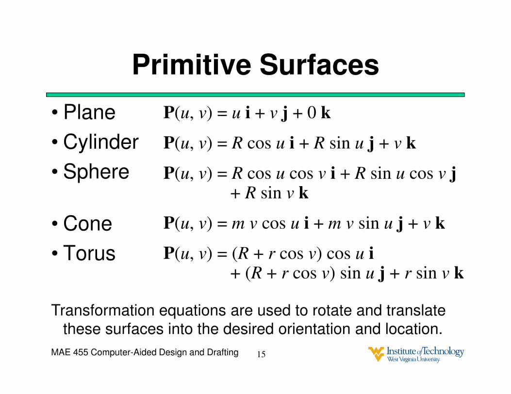
Primitive Surfaces
• Plane P(u, v) = u i + v j + 0 k
x
y
z
u
v
• Cylinder P(u, v) = R cos u i + R sin u j + v k
x
y
z
u
v
R
MAE 455 Computer-Aided Design and Drafting 15
Primitive Surfaces
• Plane
• Cylinder
• Sphere
• Cone
• Torus
P(u, v) = u i + v j + 0 k
P(u, v) = R cos u i + R sin u j + v k
P(u, v) = R cos u cos v i + R sin u cos v j+ R sin v k
P(u, v) = m v cos u i + m v sin u j + v k
P(u, v) = (R + r cos v) cos u i+ (R + r cos v) sin u j + r sin v k
Transformation equations are used to rotate and translate
these surfaces into the desired orientation and location.

MAE 455 Computer-Aided Design and Drafting 16
The B-Spline Surface
• The B-Spline surface is an extension of the B-Spline curve concept to one higher dimension.
• It uses a grid of control points, evaluated in uand v to surface points.

MAE 455 Computer-Aided Design and Drafting 17
B-Spline Surface
Properties:
• Boundaries are B-Spline curves.
• Intuitive control of surface interior.
• Derivatives (surface normals) can be evaluated
using same algorithm used to evaluate points.
• Surface is inside convex hull of control points
• NURBS surfaces can exactly represent rounded
surfaces (e.g., cylindrical and spherical surfaces).
MAE 455 Computer-Aided Design and Drafting 18
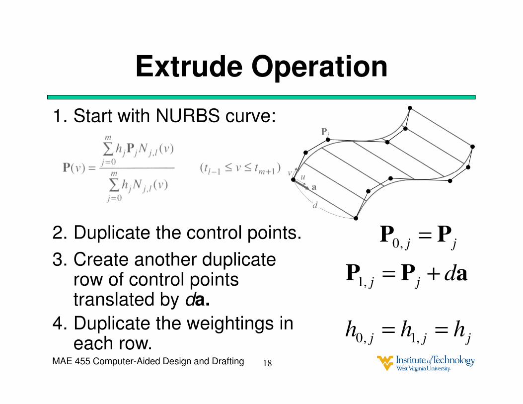
Extrude Operation
1. Start with NURBS curve:
4. Duplicate the weightings in each row. jjj hhh == ,1,0
2. Duplicate the control points.jj PP =,0
3. Create another duplicate row of control points translated by da.
aPP djj +=,1