Least-Squares Variance Component...
220
Least-Squares Variance Component Estimation: Theory and GPS Applications A.R. Amiri-Simkooei
Transcript of Least-Squares Variance Component...
Least-Squares Variance Component Estimation:
Theory and GPS Applications
A.R. Amiri-Simkooei

Least-Squares Variance Component Estimation:
Theory and GPS Applications
PROEFSCHRIFT
ter verkrijging van de graad van doctoraan de Technische Universiteit Delft,
op gezag van de Rector Magnificus prof. dr. ir. J.T. Fokkema,voorzitter van het College voor Promoties,
in het openbaar te verdedigen op maandag 2 april 2007 om 10.00 uur
door
AliReza AMIRI-SIMKOOEI
Master of Science in Geodesy EngineeringK. N. Toosi University of Technology, Tehran, Iran
geboren te Bafgh, Yazd, Iran
Dit proefschrift is goedgekeurd door de promotor:
Prof. dr. ir. P.J.G. Teunissen
Samenstelling promotiecommissie:
Rector Magnificus, voorzitterProf. dr. ir. P.J.G. Teunissen, Technische Universiteit Delft, promotorProf. dr. D.G. Simons, Technische Universiteit DelftProf. dr. ir. J.A. Mulder, Technische Universiteit DelftProf. ir. B.A.C. Ambrosius, Technische Universiteit DelftProf. P.A. Cross, University College LondonProf. R.B. Langley, University of New BrunswickDr. ir. C.C.J.M. Tiberius Technische Universiteit DelftProf. dr.-ing. habil. R. Klees, Technische Universiteit Delft, reserve
Amiri-Simkooei, AliReza
Least-squares variance component estimation: theory and GPS applications
Delft institute of Earth Observation and Space systems (DEOS),Delft University of Technology
Keywords: Least-squares variance component estimation (LS-VCE), normal distribution,elliptically contoured distribution, MINQUE, BIQUE, REML
Citation: Amiri-Simkooei, A.R. (2007). Least-squares variance component estimation:theory and GPS applications. PhD thesis, Delft University of Technology, Publication onGeodesy, 64, Netherlands Geodetic Commission, Delft
ISBN-10 90-804147-5-1ISBN-13 978-90-804147-5-4
Copyright c©2007 by Amiri-Simkooei, A.R.All rights reserved. No part of the material protected by this copyright notice may bereproduced or utilized in any form or by any means, electronic or mechanical, includingphotocopying, recording or by any information storage and retrieval system, without theprior permission of the author.
This dissertation was published with the same title in the series:Publications on Geodesy, 64, Netherlands Geodetic Commission, DelftISBN-13 978-90-6132-301-3
Typeset by the author with the LATEXDocumentation System.Printed by Optima Grafische Communicatie, The Netherlands.

In memory of my father

Abstract
Data processing in geodetic applications often relies on the least-squares method, for whichone needs a proper stochastic model of the observables. Such a realistic covariance matrixallows one first to obtain the best (minimum variance) linear unbiased estimator of theunknown parameters; second, to determine a realistic precision description of the unknowns;and, third, along with the distribution of the data, to correctly perform hypothesis testingand assess quality control measures such as reliability. In many practical applications thecovariance matrix is only partly known. The covariance matrix is then usually written as anunknown linear combination of known cofactor matrices. The estimation of the unknown(co)variance components is generally referred to as variance component estimation (VCE).
In this thesis we study the method of least-squares variance component estimation (LS-VCE) and elaborate on theoretical and practical aspects of the method. We show thatLS-VCE is a simple, flexible, and attractive VCE-method. The LS-VCE method is simplebecause it is based on the well-known principle of least-squares. With this method theestimation of the (co)variance components is based on a linear model of observation equa-tions. The method is flexible since it works with a user-defined weight matrix. Differentweight matrix classes can be defined which all automatically lead to unbiased estimatorsof (co)variance components. LS-VCE is attractive since it allows one to apply the existingbody of knowledge of least-squares theory to the problem of (co)variance component esti-mation. With this method, one can 1) obtain measures of discrepancies in the stochasticmodel, 2) determine the covariance matrix of the (co)variance components, 3) obtain theminimum variance estimator of (co)variance components by choosing the weight matrix asthe inverse of the covariance matrix, 4) take the a-priori information on the (co)variancecomponent into account, 5) solve for a nonlinear (co)variance component model, 6) applythe idea of robust estimation to (co)variance components, 7) evaluate the estimability ofthe (co)variance components, and 8) avoid the problem of obtaining negative variancecomponents.
LS-VCE is capable of unifying many of the existing VCE-methods such as MINQUE,BIQUE, and REML, which can be recovered by making appropriate choices for the weightmatrix. An important feature of the LS-VCE method is the capability of applying hypoth-esis testing to the stochastic model, for which we rely on the w-test, v-test, and overallmodel test. We aim to find an appropriate structure for the stochastic model which in-cludes the relevant noise components into the covariance matrix. The w-test statistic isintroduced to see whether or not a certain noise component is likely to be present in theobservations, which consequently can be included in the stochastic model. Based on thenormal distribution of the original observables we determine the mean and the varianceof the w-test statistic, which are zero and one, respectively. The distribution is a linearcombination of mutually independent central chi-square distributions each with one degree
ii Abstract
of freedom. This distribution can be approximated by the standard normal distribution forsome special cases. An equivalent expression for the w-test is given by introducing thev-test statistic. The goal is to decrease the number of (co)variance components of thestochastic model by testing the significance of the components. The overall model test isintroduced to generally test the appropriateness of a proposed stochastic model.
We also apply LS-VCE to real data of two GPS applications. LS-VCE is applied to theGPS geometry-free model. We present the functional and stochastic model of the GPSobservables. The variance components of different observation types, satellite elevationdependence of GPS observables’ precision, and correlation between different observationtypes are estimated by LS-VCE. We show that the precision of the GPS observables clearlydepends on the elevation angle of satellites. Also, significant correlation between observa-tion types is found. For the second application we assess the noise characteristics of timeseries of daily coordinates for permanent GPS stations. We apply LS-VCE to estimatewhite noise and power-law noise (flicker noise and random walk noise) amplitudes in thesetime series. The results confirm that the time series are highly time correlated. We alsouse the w-test statistic to find an appropriate stochastic model of GPS time series. A com-bination of white noise, autoregressive noise, and flicker noise in general best characterizesthe noise in all three position components. Unmodelled periodic effects in the data arethen captured by a set of harmonic functions, for which we rely on least-squares harmonicestimation (LS-HE) developed in the same framework as LS-VCE. The results confirm thepresence of annual and semiannual signals, as well as other significant periodic patternsin the series. To avoid the biased estimation of the variance components, such sinusoidalsignals should be included in the functional part of the model before applying LS-VCE.
Contents
Abstract i
1 Introduction 1
1.1 Background . . . . . . . . . . . . . . . . . . . . . . . . . . . . . . . . . 1
1.2 Objectives of thesis . . . . . . . . . . . . . . . . . . . . . . . . . . . . . 2
1.3 Outline of thesis . . . . . . . . . . . . . . . . . . . . . . . . . . . . . . . 3
2 Least-Squares Estimation and Validation 5
2.1 Parameter estimation in linear models . . . . . . . . . . . . . . . . . . . . 5
2.1.1 Optimal properties of estimators . . . . . . . . . . . . . . . . . . . 5
2.1.2 Model of observation equations . . . . . . . . . . . . . . . . . . . 6
2.1.3 Weighted least-squares estimation . . . . . . . . . . . . . . . . . . 7
2.1.4 Best linear unbiased estimation . . . . . . . . . . . . . . . . . . . 9
2.1.5 Maximum likelihood estimation . . . . . . . . . . . . . . . . . . . 10
2.1.6 Model of condition equations . . . . . . . . . . . . . . . . . . . . 11
2.2 Detection and validation in linear models . . . . . . . . . . . . . . . . . . 13
2.2.1 Testing simple and composite hypotheses . . . . . . . . . . . . . . 13
2.2.2 Hypothesis testing in linear models . . . . . . . . . . . . . . . . . 14
2.2.3 Overall model test . . . . . . . . . . . . . . . . . . . . . . . . . . 15
2.2.4 The w-test statistic . . . . . . . . . . . . . . . . . . . . . . . . . 16
2.2.5 The v-test statistic . . . . . . . . . . . . . . . . . . . . . . . . . . 18
2.2.6 Unknown variance of unit weight . . . . . . . . . . . . . . . . . . 19
3 Variance Component Estimation: A Review 21
3.1 Introduction . . . . . . . . . . . . . . . . . . . . . . . . . . . . . . . . . 21
3.2 Variance component model . . . . . . . . . . . . . . . . . . . . . . . . . 22
3.3 Rigorous methods . . . . . . . . . . . . . . . . . . . . . . . . . . . . . . 23
3.3.1 MINQUE method . . . . . . . . . . . . . . . . . . . . . . . . . . 23
3.3.2 BIQUE method . . . . . . . . . . . . . . . . . . . . . . . . . . . 25
3.3.3 Helmert method . . . . . . . . . . . . . . . . . . . . . . . . . . . 26
3.3.4 MLE method . . . . . . . . . . . . . . . . . . . . . . . . . . . . . 26
3.3.5 Bayesian method . . . . . . . . . . . . . . . . . . . . . . . . . . . 27
3.3.6 Non-negative methods . . . . . . . . . . . . . . . . . . . . . . . . 28
3.3.7 LS method . . . . . . . . . . . . . . . . . . . . . . . . . . . . . . 29
3.4 Simplified methods . . . . . . . . . . . . . . . . . . . . . . . . . . . . . . 30
iv Contents
3.5 Applications to geodetic data . . . . . . . . . . . . . . . . . . . . . . . . 31
4 Least-Squares Variance Component Estimation 33
4.1 Introduction and background . . . . . . . . . . . . . . . . . . . . . . . . 33
4.2 Weighted least-squares estimators . . . . . . . . . . . . . . . . . . . . . . 35
4.3 Covariance matrix of observables vh(t tT ) . . . . . . . . . . . . . . . . . . 43
4.4 Properties of least-squares estimators . . . . . . . . . . . . . . . . . . . . 45
4.4.1 Optimal properties . . . . . . . . . . . . . . . . . . . . . . . . . . 45
4.4.2 Covariance matrix of estimators . . . . . . . . . . . . . . . . . . . 46
4.4.3 Quadratic form of residuals . . . . . . . . . . . . . . . . . . . . . 47
4.4.4 Prior information . . . . . . . . . . . . . . . . . . . . . . . . . . . 48
4.4.5 Robust estimation . . . . . . . . . . . . . . . . . . . . . . . . . . 49
4.5 Minimum variance estimators . . . . . . . . . . . . . . . . . . . . . . . . 49
4.6 Maximum likelihood estimators . . . . . . . . . . . . . . . . . . . . . . . 52
4.7 In terms of model of observation equations . . . . . . . . . . . . . . . . . 53
4.7.1 Weighted least-squares estimators . . . . . . . . . . . . . . . . . . 54
4.7.2 Minimum variance estimators . . . . . . . . . . . . . . . . . . . . 55
4.7.3 Nonlinear covariance function . . . . . . . . . . . . . . . . . . . . 58
4.8 Remarks on stochastic model . . . . . . . . . . . . . . . . . . . . . . . . 60
4.8.1 Negative variance components . . . . . . . . . . . . . . . . . . . . 60
4.8.2 Singular stochastic model . . . . . . . . . . . . . . . . . . . . . . 62
4.8.3 Ill-posedness of stochastic model . . . . . . . . . . . . . . . . . . 64
4.9 Summary and concluding remarks . . . . . . . . . . . . . . . . . . . . . . 66
5 Detection and Validation in Stochastic Model 69
5.1 Introduction . . . . . . . . . . . . . . . . . . . . . . . . . . . . . . . . . 69
5.2 The w-test statistic . . . . . . . . . . . . . . . . . . . . . . . . . . . . . 69
5.2.1 Introduction . . . . . . . . . . . . . . . . . . . . . . . . . . . . . 69
5.2.2 Formulation in terms of B-model . . . . . . . . . . . . . . . . . . 71
5.2.3 Distribution of w-test statistic . . . . . . . . . . . . . . . . . . . . 74
5.2.4 Datasnooping on Qt . . . . . . . . . . . . . . . . . . . . . . . . . 77
5.2.5 Formulation in terms of A-model . . . . . . . . . . . . . . . . . . 78
5.2.6 Datasnooping on Qy . . . . . . . . . . . . . . . . . . . . . . . . . 82
5.2.7 Two illustrative examples . . . . . . . . . . . . . . . . . . . . . . 85
5.3 The v-test statistic . . . . . . . . . . . . . . . . . . . . . . . . . . . . . . 88
5.3.1 Formulation in terms of B-model . . . . . . . . . . . . . . . . . . 88
5.3.2 Formulation in terms of A-model . . . . . . . . . . . . . . . . . . 89
5.4 The overall model test . . . . . . . . . . . . . . . . . . . . . . . . . . . . 90
5.4.1 Quadratic form of residuals . . . . . . . . . . . . . . . . . . . . . 90
5.4.2 Expectation of quadratic form . . . . . . . . . . . . . . . . . . . . 92
5.4.3 Dispersion of quadratic form . . . . . . . . . . . . . . . . . . . . . 92
5.4.4 Quadratic form in case p = 1 . . . . . . . . . . . . . . . . . . . . 93
5.4.5 Approximation of quadratic form . . . . . . . . . . . . . . . . . . 95
5.5 Summary and concluding remarks . . . . . . . . . . . . . . . . . . . . . . 98
Contents v
6 Multivariate Variance-Covariance Analysis 99
6.1 Introduction . . . . . . . . . . . . . . . . . . . . . . . . . . . . . . . . . 99
6.2 Multivariate parameter estimation . . . . . . . . . . . . . . . . . . . . . . 100
6.3 Multivariate variance-covariance estimation . . . . . . . . . . . . . . . . . 101
6.4 Multivariate variance-covariance validation . . . . . . . . . . . . . . . . . 104
6.4.1 The w-test statistic . . . . . . . . . . . . . . . . . . . . . . . . . 104
6.4.2 The v-test statistic . . . . . . . . . . . . . . . . . . . . . . . . . . 106
6.4.3 Overall model test . . . . . . . . . . . . . . . . . . . . . . . . . . 112
7 GPS Geometry-Free Model 113
7.1 Introduction . . . . . . . . . . . . . . . . . . . . . . . . . . . . . . . . . 113
7.2 Functional and stochastic models . . . . . . . . . . . . . . . . . . . . . . 113
7.3 Sophisticated stochastic models . . . . . . . . . . . . . . . . . . . . . . . 116
7.3.1 Satellite elevation dependence . . . . . . . . . . . . . . . . . . . . 116
7.3.2 Correlation between observation types . . . . . . . . . . . . . . . . 116
7.3.3 Time correlation of observables . . . . . . . . . . . . . . . . . . . 118
7.4 Multivariate linear model . . . . . . . . . . . . . . . . . . . . . . . . . . . 119
7.5 Presentation and interpretation of results . . . . . . . . . . . . . . . . . . 120
7.6 Numerical results . . . . . . . . . . . . . . . . . . . . . . . . . . . . . . . 121
7.6.1 Experiment description . . . . . . . . . . . . . . . . . . . . . . . . 121
7.6.2 Variances of observation types . . . . . . . . . . . . . . . . . . . . 122
7.6.3 Covariances between code observations . . . . . . . . . . . . . . . 124
7.6.4 Single channel variances . . . . . . . . . . . . . . . . . . . . . . . 127
7.7 Summary and conclusions . . . . . . . . . . . . . . . . . . . . . . . . . . 130
8 GPS Coordinate Time Series 131
8.1 Introduction . . . . . . . . . . . . . . . . . . . . . . . . . . . . . . . . . 131
8.2 Review of previous work . . . . . . . . . . . . . . . . . . . . . . . . . . . 131
8.3 Analysis of GPS coordinate time series . . . . . . . . . . . . . . . . . . . 133
8.3.1 Introduction to noise process . . . . . . . . . . . . . . . . . . . . 133
8.3.2 Functional model . . . . . . . . . . . . . . . . . . . . . . . . . . . 134
8.3.3 Stochastic model . . . . . . . . . . . . . . . . . . . . . . . . . . . 134
8.3.4 Misspecification in functional and stochastic model . . . . . . . . . 135
8.4 Model identification . . . . . . . . . . . . . . . . . . . . . . . . . . . . . 136
8.4.1 Least-squares harmonic estimation (LS-HE) . . . . . . . . . . . . . 136
8.4.2 The w-test statistic . . . . . . . . . . . . . . . . . . . . . . . . . 138
8.4.3 Demonstration using simulated data . . . . . . . . . . . . . . . . . 139
8.5 Numerical results and discussions . . . . . . . . . . . . . . . . . . . . . . 141
8.5.1 Data and model description . . . . . . . . . . . . . . . . . . . . . 141
8.5.2 Variance component analysis . . . . . . . . . . . . . . . . . . . . 141
8.5.3 Functional model . . . . . . . . . . . . . . . . . . . . . . . . . . . 143
8.5.4 Stochastic model . . . . . . . . . . . . . . . . . . . . . . . . . . . 148
8.5.5 Remarks and discussions . . . . . . . . . . . . . . . . . . . . . . . 152
8.5.6 Error estimate of parameters . . . . . . . . . . . . . . . . . . . . 155
8.6 Summary and conclusions . . . . . . . . . . . . . . . . . . . . . . . . . . 156
vi Contents
9 Conclusions and Recommendations 159
9.1 Introduction . . . . . . . . . . . . . . . . . . . . . . . . . . . . . . . . . 159
9.2 Summary . . . . . . . . . . . . . . . . . . . . . . . . . . . . . . . . . . . 159
9.3 Conclusions . . . . . . . . . . . . . . . . . . . . . . . . . . . . . . . . . . 161
9.4 Recommendations . . . . . . . . . . . . . . . . . . . . . . . . . . . . . . 163
A Mathematical Background 165
A.1 Trace, Kronecker product and vec operator . . . . . . . . . . . . . . . . . 165
A.2 Duplication and commutation matrices . . . . . . . . . . . . . . . . . . . 165
B Derivation of Equations 167
B.1 Equation (5.116) . . . . . . . . . . . . . . . . . . . . . . . . . . . . . . . 167
B.2 Equation (5.123) . . . . . . . . . . . . . . . . . . . . . . . . . . . . . . . 168
B.3 Equation (5.158) . . . . . . . . . . . . . . . . . . . . . . . . . . . . . . . 169
B.4 Equation (5.159) . . . . . . . . . . . . . . . . . . . . . . . . . . . . . . . 169
B.5 Equation (5.174) . . . . . . . . . . . . . . . . . . . . . . . . . . . . . . . 171
C Moments of Normally Distributed Data 173
C.1 Moment generating function . . . . . . . . . . . . . . . . . . . . . . . . . 173
C.2 Moment generating function for normal distribution . . . . . . . . . . . . 173
C.3 First four moments of normally distributed data . . . . . . . . . . . . . . 174
C.4 Sixth and eighth central moments . . . . . . . . . . . . . . . . . . . . . . 175
C.5 Quadratic forms in normal variables . . . . . . . . . . . . . . . . . . . . . 176
C.6 Multiplication of four quadratic forms . . . . . . . . . . . . . . . . . . . . 177
D Mixed model with hard constraints 181
D.1 Model representation E{y} = Ax with BT x = c . . . . . . . . . . . . . . 181
D.2 Parameter significance test (v-test) . . . . . . . . . . . . . . . . . . . . . 183
D.3 Derivation of w-test from v-test statistic . . . . . . . . . . . . . . . . . . 184
Bibliography 185
Index 195
Notation and Symbols 199
Abstract (in Dutch) 203
Curriculum Vitae 205
Acknowledgements 207
Introduction 11.1 Background
Data processing in geodetic applications usually relies on the least-squares method, orequivalently, when the inverse of the covariance matrix of observables is taken as theweight matrix, the best linear unbiased estimation (BLUE). To that end we deal with twomodels, namely, ‘functional model’ and ‘stochastic model’. The former is usually eitherwell-known or subject to extensive research, and the latter, containing the second-ordercentral moments of the observables receives far less attention. Statistical models in use forinstance in the fields of Global Navigation Satellite Systems (GNSS) positioning applica-tions are usually simple and rudimentary. For many applications, it is of importance to haveinformation available on the covariance matrix of an observable random vector. Such infor-mation allows one to study the different contributing factors of the errors in observations,to properly describe the precision of functions of interest by means of application of thecovariance propagation law, and to obtain minimum variance estimators of the parametersin a linear model. This will also allow one to correctly perform hypothesis testing and toassess other quality control measures such as reliability.
An adequate statistical model is thus needed to arrive at a proper description of theestimators’ quality. Incomplete knowledge of the covariance matrix of the observablesoccurs in many of the GNSS applications. Often, however, the covariance matrix of theobservables is only partly known, as a consequence of which the unknown part needs to beestimated from the redundant observables. The estimation of these unknown componentsof a covariance matrix is generally referred to as variance component estimation (VCE).Various VCE-studies have been conducted to improve our knowledge of the GNSS stochasticmodel. Variance component estimation is also an important issue in other geodetic fields ofapplication, in particular in applications where heterogeneous data needs to be combined.An example where the heterogeneous data should be combined is the combination of InSARand leveling data. Another example is the combination of classical geodesy networks andGPS networks.
Methods for estimating (co)variance components have been intensively investigated inthe statistical and geodetic literature. There exist many different methods for variancecomponent estimation. The methods differ in the estimation principle employed, as wellas in the distributional assumptions that need to be made. Most methods have beendevised for the linear model, for which one assumes that the covariance matrix of theobservables can be written as an unknown linear combination of known cofactor matrices.The coefficients of this linear combination are then the unknown (co)variance componentsthat need to be estimated. Of the leading variance component estimators, we mentionthe minimum norm quadratic unbiased estimator (MINQUE), the best invariant quadratic
2 Chapter 1. Introduction
unbiased estimator (BIQUE), the least-squares variance component estimator (LS-VCE),the restricted maximum likelihood estimator (REML), and the Bayesian method to VCE.
The MINQUE method is one of the more commonly used methods for estimation ofvariance components. Apart from the first and second order moments of the observables,this method does not require any distributional assumptions. The BIQUE, however, doesrequire knowledge of some of the higher order moments. This minimum variance quadraticestimator has been derived and studied, under the assumption of normally distributedobservables. The LS-VCE method is based on the least-squares principle and works witha user-defined weight matrix. As such the method only requires information on the firstand second order moments. The REML method and the Bayesian method, both requirein contrast to the other methods, complete information on the probability density functionof the observables. Using the normal distribution, maximum likelihood estimators andBayesian estimators have been derived and studied by different authors.
1.2 Objectives of thesis
In this thesis we further study and use the least-squares variance component estimation(LS-VCE) which was originally developed by Teunissen (1988). For a review see Teunissenand Amiri-Simkooei (2006). Since the method can be applied to many modern geodeticapplications, this thesis elaborates this theory in much detail. Although the method isprobably one of the lesser known VCE-methods, we will show that it is a simple, flexibleand attractive method for the estimation of unknown variance and covariance components.
• The method is simple, since it is based on the principle of least-squares. This will leadus to use one unified estimation principle, namely the well-known and well-understoodleast-squares principle, for both the functional and stochastic model.
• The method is flexible, since it works with a user-defined weight matrix. Theweighted LS-VCE does not need any distributional assumption for the observables.The weighted LS-VCE is formulated in a linear model and thus leads to unbiased(co)variance component estimators. In case of elliptical distributions which includefor instance the normal distribution, the method can automatically produce minimumvariance estimators.
• The method of LS-VCE is attractive, since it allows one to directly apply the existingbody of knowledge of least-squares theory. In this thesis we present the LS-VCEmethod for different scenarios and explore its various properties. All other methodsof VCE, for instance, concern only the estimation of (co)variance components. But,LS-VCE allows one also to apply hypothesis testing to the stochastic model which isconsidered to be a distinguished feature of this method.
Being a least-squares estimator, the LS-VCE automatically inherits all the well-knownproperties of a least-squares estimator. We show how the existing body of knowledge ofleast-squares theory can be used to one’s advantage for studying various aspects of VCE.For example, since the method is based on the least-squares principle, the precision of(co)variance estimators can directly be obtained.
We include various examples to illustrate this theory at work and address implementationaspects. Application of LS-VCE to real GPS data will be considered as well. We will use
1.3 Outline of thesis 3
LS-VCE to study the stochastics of GPS code and carrier phase data and also of GPScoordinate time series.
1.3 Outline of thesis
This thesis is organized as follows:Chapter 2 explains the least-squares estimation and validation in a general linear model
of observation equations. Three estimation principles, which lead to the weighted least-squares estimation, the best linear unbiased estimation (BLUE), and the maximum likeli-hood estimation, will be discussed. Equivalent expressions for estimators are determinedusing the model of condition equations afterward. The last part of this chapter deals withhypotheses testing to find misspecifications (with respect to data) in a linear model. Thisincludes two types of equivalent tests: the observation test and the parameter significancetest. For this purpose the overall model test, the w-test statistic, and the v-test statisticwill be addressed. Detection of observation outliers is a prerequisite for obtaining unbiased(co)variance estimators.
Chapter 3 briefly reviews various (co)variance component estimation principles. Westart from elementary error sources and construct a variance component model. Wethen apply different principles like unbiasedness, minimum norm, minimum variance, andmaximum likelihood to this model to obtain various estimators. This includes minimumnorm quadratic unbiased estimators (MINQUE), best invariance quadratic unbiased esti-mators (BIQUE), the Helmert method to VCE, maximum likelihood estimators (MLE),the Bayesian method to VCE, and least-squares estimators. These methods differ in theestimation principles as well as in the distributional assumptions. We will present the under-lying assumptions of each method. We then discuss simple and approximate VCE methodswhich need less computational load when compared to the rigorous methods.
Chapter 4 introduces the principle of weighted least-squares for the estimation of un-known (co)variance components. We formulate a linear (co)variance component model,define the least-squares variance component estimator and determine its covariance matrix.We consider the weighted LS-VCE method for a special class of weight matrices. Basedon this weight matrix class we then show how the LS-VCE can be turned into a minimumvariance VCE. We also show how the existing body of knowledge of least-squares theorycan be used to one’s advantage for studying and solving various aspects of the variancecomponent estimation problem. Topics that are addressed are: measures of inconsistency,the use of a-priori variance component information, nonlinear variance component estima-tion, and robust and non-negative variance component estimation. Later, in this chapterwe make some comments, supported by a few examples, on the estimability of (co)variancecomponents.
In chapter 5 we apply hypothesis testing to the stochastic model. The w-test, the v-test,and the overall model test will be generalized for the stochastic model. It is aimed to findmisspecifications in the stochastic model, to improve an existing stochastic model, andto judge whether or not (or which) additional (co)variance components are likely to beincluded in (or excluded from) the stochastic model. We will derive the distribution of thew-test and the v-test statistics under the normality assumption of the original observables.For the overall model test statistic, the distribution is complicated. We thus only obtain thefirst and the second order moments, instead of its complete distribution. However, using
4 Chapter 1. Introduction
an approximation we show how the overall model test of the stochastic model is convertedto the overall model test of the functional model.
Chapter 6 deals with multivariate parameter and variance-covariance estimation andvalidation. We aim to apply the theory on least-squares estimation of (co)variance compo-nents introduced in chapter 4, and to apply the idea of detection and validation introducedin chapter 5, to a multivariate linear model of observation equations. We show that theestimators in the multivariate model can be considered as a generalization of the estimatorsin the univariate model. This holds in fact for the w-test and the v-test statistics as wellas for their related distributions. We also show, when the redundancy of the model islarge enough, that the distribution of the test statistics can be approximated by a normaldistribution.
Chapters 7 and 8 present numerical results of application of LS-VCE to real GPS data.Chapter 7 deals with the GPS geometry-free observation model for which LS-VCE is usedto assess the stochastics of GPS pseudorange and carrier-phase data. The purpose of thischapter is to come up with a realistic and adequate covariance matrix of GPS observables.Topics that will be addressed are: the precision of different code and phase observations,satellite elevation dependence of the observable’s precision, and the correlation betweendifferent code and phase observations. Chapter 8 concerns coordinate time series analysisof permanent GPS stations. We discuss both the functional model and the stochasticmodel in detail. We will then introduce the least-squares harmonic estimation (LS-HE) tocome up with an appropriate functional model by introducing a set of harmonic functionsto compensate for unmodelled effects in the data series. We then apply the LS-VCE toestimate different noise components (white noise, flicker noise, and random walk noise)of the series. We also employ the w-test, in conjunction with LS-VCE, to come up withan appropriate stochastic model for GPS time series. Other topics like misspecifications inboth the functional and the stochastic model, and duality between these two models areaddressed as well.
Finally, chapter 9 reviews the conclusions of this work and presents recommendationsfor further research.
Least-Squares Estimation and Validation 22.1 Parameter estimation in linear models
2.1.1 Optimal properties of estimators
This chapter reviews in general the theory of least-squares estimation and validation in aninconsistent linear model where the inconsistency is caused by errors in the data. Fromexperience we know that various uncertain phenomena can be modeled as a random variable(or a random vector), namely y. An example is the uncertainty in instrument readingsdue to measurement errors. The randomness of y is expressed by its probability densityfunction (PDF). In practice, our knowledge of the PDF is incomplete. The PDF can usuallybe indexed with one or more unknown parameters. The PDF of a random m-vector y isdenoted as fy(y|x), in which x is an n-vector of unknown parameters to be estimated. Theapproach is to take an observation of the m-vector y and to use this observation vectorto estimate the unknown n-vector x. The observation y as a realization of y with PDFfy(y|x) contains information about x which can be used to estimate its value.
We thus require to determine x from an observation vector y. The essential estimationproblem is therefore to find a function G : R
m 7→ Rn, such that x = G(y) can be taken
as our estimate of x. In fact, if we apply G to y, we obtain the random vector x = G(y).The random vector x is called the estimator of x and x is called the estimate of x. Theestimator is a random vector which has its own probability density function (distribution),while, the estimate is a realized value of the estimator and thus a deterministic vector.The difference ǫ = x − x is called the estimation error. Since x depends on the chosenfunction G, the estimation error depends on G as well. We list three desirable propertiesfor ǫ which all express in some sense the closeness of x to x. Such properties can be usedas criteria for finding an ’optimal’ function G.
Unbiasedness The estimator x is said to be an unbiased estimator of x if and only ifthe mathematical expectation of the estimation error is zero. An estimator is thereforeunbiased if the mean of its distribution equals x
E{x} = x for all x , (2.1)
where E{.} denotes the expectation operator. This implies that the average of repeatedrealizations of ǫ will tend to zero on the long run. An estimator which is not unbiased issaid to be biased and the difference E{ǫ} = E{x} − x is called the bias of the estimator.The size of the bias is therefore a measure of closeness of x to x. The mean error E{ǫ} isa measure of closeness that makes use of the first moment of the distribution of x.

6 Chapter 2. Least-Squares Estimation and Validation
Minimum variance (best) A second measure of closeness of the estimator to x is themean squared error (MSE), which is defined as
MSE = E{‖x− x‖2
}→ min , (2.2)
where ‖.‖ is a vector norm. If we were to compare different estimators by looking at theirrespective MSEs, we would prefer one with small or the smallest MSE. This is a measureof closeness that makes use also of the second moment of the distribution of x. The ’best’estimator, in the absence of biases, therefore is of minimum variance.
Maximum likelihood Rather than relying on the first two moments of a distribution, onecan also define what closeness means in terms of the distribution itself. As a third measureof closeness we therefore consider the probability that the estimator x resides in a smallregion centered at x. If we take this region to be a hypersphere with a given radius r, themeasure is given as
P(‖x− x‖2 ≤ r2
)→ max . (2.3)
If we were to compare different estimators by looking at their respective values for proba-bility (2.3), we would prefer one with large or the largest such probability. Unfortunately itis rarely possible to derive an estimator which has the largest such probability for all x.
2.1.2 Model of observation equations
There are different estimation methods that we discuss in this chapter. The simplestmethod that one can apply needs information about the first moment of the distribution.Since the PDF depends on the unknown parameter x, the mean will generally depend on xas well. We will however assume that we know how the mean depends on x. The relationis through a mapping A : R
n 7→ Rm. In the linear(ized) case A is an m× n matrix.
Redundancy Redundant measurements are often taken to increase the accuracy of theobtained results and to check for the presence of blunders (i.e. m > n). Due to intrinsicuncertainty in observations, redundant measurements generally lead to an inconsistentsystem of equations. For m > n such an inconsistent linear system of equations has theform y ≈ Ax. This linear system of equations for which m > n = rank(A) is also referredto as an overdetermined system. The number b = m− rank(A) = m− n is referred to asthe redundancy of the system (or redundancy of the functional model).
Least-squares principle It is well known that an inconsistent system has no solutionx that can reproduce y. As a first step one can make the system consistent by adding ameasurement error vector e: y = Ax+e. But now we have m+n unknowns in m equations,and therefore an infinite number of possible solutions for x and e (underdetermined system).It seems reasonable to select from this infinite set of possible solutions, the solution whichin some sense gives the smallest value for e. This implies choosing the solution for x suchthat Ax is, in some sense, as close as possible to the measurement vector y. The (weighted)least-squares (LS) principle states to minimize the (weighted) norm of the residual vectore, namely ‖e‖2W = eT We = (y−Ax)T W (y−Ax), where ‖.‖ denotes the norm of a vectorand W is the weight matrix. Any symmetric and positive-definite matrix is considered tobe in the class of admissible weight matrix W (see Teunissen et al., 2005).
2.1 Parameter estimation in linear models 7
Linear model From now on we will refer to the linear system of equations y = Ax + e asthe linear model of observation equations which is denoted as
E{y} = Ax , W, or D{y} = Qy , (2.4)
where y is the m-vector of (stochastic) observables, A is the m × n design matrix, x isthe n-vector of unknown parameters, and W and Qy are the m × m weight matrix andcovariance matrix of the observables, respectively. The design matrix A is assumed tobe of full column rank, i.e., rank(A) = n, provided that m ≥ n, and W and Qy aresymmetric and positive-definite. Again E{.} denotes the expectation operator, and D{.}the dispersion operator. The above parametric form of the functional model is referred toas a Gauss-Markov model when y is normally distributed, i.e. y ∼ N(Ax,Qy).
Estimation methods Three different estimation methods will be treated in this chap-ter. They are: weighted least-squares estimation (WLSE), best linear unbiased estimation(BLUE) and maximum likelihood estimation (MLE). The methods differ not only in theestimation principles involved, but also in the information that is required about the PDFfy(y|x). WLSE is applied when we only have information about the first moment of thedistribution. BLUE is a method which can be applied when we have information about thefirst two moments of the distribution. MLE is used if we know the complete structure ofthe PDF fy(y|x). An important example for which the complete structure of the PDF isknown is the multivariate normal distribution, i.e. as y ∼ Nm(Ax,Qy).
2.1.3 Weighted least-squares estimation
Definition 2.1 (Weighted least-squares) Let E{y} = Ax, with A an m× n matrix ofrank(A) = n, be a possibly inconsistent linear model of observation equations and let Wbe a symmetric and positive-definite m × m weight matrix (W = W T > 0). Then theweighted least-squares solution of the system is defined as
x = arg minx∈Rn
(y − Ax)T W (y − Ax) . (2.5)
The difference e = y − Ax is called the (weighted) least-squares residual vector. Itssquared (weighted) norm ‖e‖2W = eT We is a scalar measure for the inconsistency of thelinear system. �
Estimator Since the mean of y depends on the unknown x, also the PDF of y dependson the unknown x. The problem of determining a value for x can thus now be seen as anestimation problem, i.e. as the problem of finding a function G such that x = G(y) canact as the estimate of x and x = G(y) as the estimator of x. The weighted least-squaresestimator (WLSE) is given as (Teunissen et al., 2005)
x = (AT WA)−1AT Wy , (2.6)
which is a linear estimator, since all the entries of x are linear combinations of the entriesof y. The least-squares estimator y = Ax of observables and e = y − y of residuals followfrom equation y = Ax + e as
{y = PAy ;e = P⊥
A y ,(2.7)
8 Chapter 2. Least-Squares Estimation and Validation
with PA = A(AT WA)−1AT W and P⊥A = Im − PA two (orthogonal) projectors. The
projector PA projects onto the range space of A (i.e. R(A)), and along its orthogonalcomplement (i.e. R(A)⊥), while P⊥
A projects onto R(A)⊥ and along R(A). R(.) denotesthe range space of a matrix. For some useful properties of these two projectors refer toTeunissen (2000a).
Unbiasedness To get some insight in the performance of an estimator, we need to knowhow the estimator relates to its target value. Based on the assumption E{e} = 0, theexpectations of x, y and e follow as
E{x} = x , E{y} = E{y} = Ax , E{e} = E{e} = 0 . (2.8)
This shows that the WLSE is an linear unbiased estimator (LUE). Unbiasedness is clearlya desirable property. It implies that on the average the outcomes of the estimator will beon target. Also y and e are on target on the average. Note that the unbiasedness of theWLSE is independent of the choice made for the weight matrix W .
Covariance matrix In order to obtain the covariance matrices of x, y and e, we need thecovariance matrix of e or observables y, namely Qy. The covariance matrices of x, y ande will be denoted respectively as Qx, Qy and Qe. Application of the error propagation lawto equations (2.6) and (2.7) yields
Qx = (AT WA)−1AT WQyWA(AT WA)−1 ;Qy = PAQyP
TA ;
Qe = P⊥A QyP
⊥TA .
(2.9)
These covariance matrices depend on the choice made for the weight matrix W .
Mean squared error The mean and the covariance matrix of an estimator come togetherin the mean squared error of the estimator. As before, let ǫ = x − x be the estimationerror. Assume that we ’measure’ the size of the estimation error by the expectation of thesum of squares of its entries, E{ǫT ǫ} = E{‖x − x‖2}, which is called the mean squarederror (MSE) of the estimator. It can easily be shown that the MSE is decomposed asE{‖x − x‖2} = E{‖x − E{x}‖2} + E{‖x − E{x}‖2}. The first term on the right-handside is the trace of the covariance matrix of the estimator and the second term is thesquared norm of the bias of the estimator. But since the WLSE is unbiased, the secondterm vanishes, as a result of which the MSE of the WLSE reads
E{‖x− x‖2} = tr(Qx) . (2.10)
Quadratic form of residuals In weighted least-squares, one important criterion whichshows the inconsistency of the linear model of observation equations is the quadratic form(squared norm) of the residuals which is given as
‖e‖2W = eT We = yT Wy − yT WA(AT WA)−1AT Wy . (2.11)
Note 2.1 The results in equations (2.8), (2.9), (2.10) and (2.11) are all independent ofthe unspecified distribution of y. The unbiasedness property (2.8) is even independent ofthe choice made for the weight matrix W , while the covariance matrices (2.9), the meansquared error (2.10), and the quadratic form (2.11) depend on W . One may thereforethink of the ’best’ weight matrix that minimizes the MSE (see next section). ⊡
2.1 Parameter estimation in linear models 9
Normality The random vectors x, y and e are all linear functions of y. This impliesthat they have a Gaussian (normal) distribution whenever y has a normal distribution.Therefore, if y has a normal distribution, i.e. y ∼ Nm(Ax,Qy) then
x ∼ Nn(x,Qx); y ∼ Nm(Ax,Qy); e ∼ Nm(0, Qe) . (2.12)
Note, since the covariance matrix Qe is singular, that the least-squares residual vector ehas a singular normal distribution. Also note that the first two distributions differ from thethird in the sense that their means are unknown. Therefore, if Qy is given, only the shapeof their PDFs is known, but not the location. The PDF of e, however, is completely knownonce Qy is given. This property will turn out to play an important role in section 2.2.
2.1.4 Best linear unbiased estimation
Minimum MSE The weighted least-squares approach was introduced as an appealingtechnique for solving an inconsistent system of equations. The method itself is a deter-ministic principle, since no concepts from probability theory are used in formulating theleast-squares minimization problem. In order to select an optimal estimator from the classof linear unbiased estimators (LUE), we need to define the optimality criterion. As optimal-ity criterion we choose the minimization of the mean squared error (MSE). The estimatorwhich has the smallest mean squared error of all LUEs is called the best linear unbiasedestimator (BLUE). Such a minimization problem results in the smallest possible variancefor estimators, i.e. E{‖x− x‖2} = tr(Qx) ≡ min.
Estimator If the covariance matrix Qy of the observables is known, one could use thebest linear unbiased estimation (BLUE) by taking the weight matrix to be the inverse ofthe covariance matrix, namely taking W = Q−1
y in equations (2.6) and (2.7). With thisthe BLUE estimators of x, y, and e in equation y = Ax + e read
x = (AT Q−1y A)−1AT Q−1
y y ;y = PAy ;e = P⊥
A y .(2.13)
where both PA = A(AT Q−1y A)−1AT Q−1
y and P⊥A = Im − PA are orthogonal projectors.
Substitution of W = Q−1y into equation (2.9) yields the covariance matrix of the BLUE
estimators as
Qx = (AT Q−1y A)−1 ;
Qy = PAQy ;Qe = P⊥
A Qy .(2.14)
It can be shown that of all linear unbiased estimators, the BLUE-estimator has minimumvariance. It is therefore a minimum variance linear unbiased estimator. The BLUE isalso sometimes called the probabilistic least-squares estimator. The property of minimumvariance is also independent of the distribution of y (like the unbiasedness property). Inthe literature, the choice of W = Q−1
y , leading to the BLUE, is often made by default. Inthe thesis, in general, we will treat the weighted least-squares estimators and the BLUE tobe different.
10 Chapter 2. Least-Squares Estimation and Validation
Quadratic form of residuals From the BLUE estimators, the inconsistency criterion ofthe linear model of observation equations, expressed by the quadratic form of the residuals,is given as
‖e‖2Q−1
y= eT Q−1
y e = yT Q−1y y − yT Q−1
y A(AT Q−1y A)−1AT Q−1
y y . (2.15)
The preceding squared norm of the residuals will play an important role in section ofdetection and validation (section 2.2).
Note 2.2 In the weighted least-squares the weight matrix W plays the role of a metrictensor in a vector space. The BLUE estimators take the weight matrix as the inverse of thecovariance matrix. Therefore, the covariance matrix of the observables is closely relatedto the metric tensor. We have thus some probabilistic interpretations in our vector space.For example if the covariances between observables are zero, this means that the standardbasis vectors of the vector space are orthogonal ; uncorrelated observables mean, for basisvectors, having no projection on each other. If in addition the variances are equal, thismeans that the basis vectors are orthonormal . Therefore, if we take the weight matrix asthe inverse of covariance matrix, the definition of the minimum distance (minimum norm)in the vector space obtained from weighted least-squares will coincide with the definitionof minimum variance in the stochastic model (space) obtained from BLUE. ⊡
2.1.5 Maximum likelihood estimation
So far we have seen two different estimation methods at work: WLSE and BLUE. Thesetwo methods are not only based on different principles, but they also differ in the type ofinformation that is required of the PDF of y. For WLSE we only need information aboutthe first moment of the PDF, the mean of y. For BLUE we need additional information.Apart from the first moment, we also need the second (central) moment of the PDF, thecovariance matrix of y. For the linear model, the two principles give identical results whenthe weight matrix is taken equal to the inverse of the covariance matrix. In this section weintroduce the method of maximum likelihood estimation (MLE) which requires knowledgeof the complete PDF.
The principle The maximum likelihood (ML) method is conceptually one of the simplestmethods of estimation. It is only applicable however when the general structure of the PDFis known. Assume therefore that the PDF of y ∈ R
m, i.e. fy(y|x), is known apart fromsome n unknown parameters. Since the PDF will change when x changes, we in fact havea whole family of PDFs in which each member of the family is determined by the valuetaken by x. Since x is unknown, it is not known to which PDF an observed value of y, i.e.y0, belongs. The idea now is to select from the family of PDFs, the PDF which gives thebest support of the observed data. For this purpose one considers fy(y0|x) as function ofx. This function is referred to as the likelihood function of y0 which produces, as x varies,the probability densities of all the PDFs for the same sample value y0. Would x be thecorrect value, then the probability of y being an element of an infinitesimal region centeredat y0 is given as fy(y0|x)dy. A reasonable choice for x, given the observed value y0, istherefore the value which corresponds with the largest probability, maxx fy(y0|x)dy, andthus with the largest value of the likelihood function. The maximum likelihood estimator(MLE) of x is therefore defined as follows:
2.1 Parameter estimation in linear models 11
Definition 2.2 (Maximum likelihood) Let the PDF of the vector of observables y ∈ Rm
be parameterized as fy(y|x), with x ∈ Rn unknown. Then the MLE of x is given as
x = arg maxx∈Rn
fy(y|x). � (2.16)
The computation of the maximum likelihood solution may not always be an easy task. Ifthe likelihood function is sufficiently smooth, the two necessary and sufficient conditionsfor x to be a (local or global) maximizer are
∂xfy(y|x) = 0 ; and ∂2xxT fy(y|x) < 0 , (2.17)
with ∂x and ∂2xxT the first and the second order partial derivatives with respect to x,
respectively. Therefore, the gradient has to be zero and the Hessian matrix (the symmetricmatrix of second-order partial derivatives) has to be negative definite. For more informationsee Teunissen et al. (2005).
Note 2.3 (MLE and BLUE) In case of normally distributed data (Gauss-Markovmodel), the MLE estimators are identical to the BLUE ones. Let y ∼ Nm(Ax,Qy), with
x the n-vector of unknown parameters. Then fy(y|x) = (det(2πQy))−1/2 exp{−1
2‖y −
Ax‖2Q−1
y}, from which it follows that arg maxx∈Rn fy(y|x) = arg minx∈Rn ‖y − Ax‖2
Q−1y
.
Therefore, x = (AT Q−1y A)−1AT Q−1
y y. The estimators y and e as well as their covariancematrices are also the same as those given for BLUE estimators (see previous section).
2.1.6 Model of condition equations
Relations between variables can be expressed in various equivalent forms. Two primeexamples are the so-called parametric form and the implicit form. So far we have expressedthe linear model in the form E{y} = Ax. This is the so-called parametric form of thelinear model (model of observation equations). The mean of y is explicitly parameterizedin terms of the unknown parameter vector x. Although this is the most common form ofthe linear model, other equivalent formulations exist. For example, one can also includesome hard constraints into this model (see appendix D.1). We can enumerate at leastother forms like the conditioned model and combined (mixed) model. The implicit form ofthe linear model is called the conditioned linear model. In this chapter we restrict ourselvesonly to the model of condition equations. This model describes the conditions which aresatisfied by the entries of the mean vector E{y}. For this formulation we will give thecorresponding expressions for the BLUE estimators.
Linear model Each parametric linear model E{y} = Ax has its equivalent conditionedlinear model. The model of parametric equations can be rewritten in terms of the modelof condition equations as
BT y = t , E{t} = 0 , Qt = D{t} = BT QyB , (2.18)
with B a given m× b matrix, and Qt the b× b covariance matrix of misclosure b-vector t.The vector of misclosures provides a direct measure for inconsistency. The matrix B hasfull column rank, i.e., rank(B) = b provided that b ≤ m, which is always true since b, theredundancy of the functional model, is given as b = m− n. The matrix Qt is assumed tobe symmetric and positive-definite.
12 Chapter 2. Least-Squares Estimation and Validation
Relation with A Each additional observation on top of the n-number of observationswhich are needed for the unique determination of the unknown parameters x in the linearmodel E{y} = Ax leads to an extra condition equation. For example, the height differencesof a closed loop in leveling should sum up to zero. Or three interior angles of a triangleshould always add up to π. The matrix B is constructed on the basis of these independentconditions which the redundant observations have to fulfill. It should be pointed out thatobtaining the condition equations and the B matrix is sometimes difficult. The followingrelation is always true between two matrices A and B
BT A = 0 , (2.19)
which means that the columns of the matrix B are complementary and orthogonal to thecolumns of the matrix A. That is, R(B) = N (AT ) which means that R(A)⊕R(B) = R
m
and R(A) ⊥ R(B), where R(.) denotes the range space of a matrix, N (.) the null spaceand ⊕ denotes the direct sum of the two subspaces.
Estimator In order to obtain the BLUE estimator, we will use the following identity:
A(AT Q−1y A)−1AT Q−1
y + QyB(BT QyB)−1BT = Im . (2.20)
For a proof see Teunissen et al. (2005). According to this matrix identity, we have for theorthogonal projector PA = A(AT Q−1
y A)−1AT Q−1y and P⊥
A = I − A(AT Q−1y A)−1AT Q−1
y
equivalent expressions in terms of the model of condition equations (B-model)
PA = P⊥QyB = I −QyB(BT QyB)−1BT ;
P⊥A = PQyB = QyB(BT QyB)−1BT ,
(2.21)
where P⊥QyB is an orthogonal projector which projects onto R(QyB)⊥ and along R(B) and
PQyB projects onto R(B) and along R(QyB)⊥. From equation (2.18), the least-squaresestimator (BLUE) of the observables and residuals is obtained as
y = P⊥QyBy ; e = PQyBy , (2.22)
with the covariance matrices of the form
Qy = P⊥QyBQy, Qe = PQyBQy. (2.23)
Quadratic form of misclosures The vector of misclosures has a direct link with theBLUE’s residual vector. The BLUE’s residual vector e = y − y and its squared norm‖e‖2
Q−1y
can be expressed in the vector of misclosures as
e = QyBQ−1t t ; ‖e‖2
Q−1y
= ‖t‖2Q−1
t= tT Q−1
t t . (2.24)
Note 2.4 The formulas of the weighted least-squares estimators of section 2.1.3 can alsobe obtained for the model of condition equations. For this purpose we need to define theprojectors PA and P⊥
A as P⊥W−1B and PW−1B, respectively, where Qy is substituted by W−1
in projectors (2.21) .
2.2 Detection and validation in linear models 13
2.2 Detection and validation in linear models
2.2.1 Testing simple and composite hypotheses
Most powerful test The simple likelihood ratio (SLR) test is derived based on theNeyman-Pearson testing principle. This principle states to choose, among all tests orcritical regions possessing the same size type I error, α, the one for which the size of thetype II error, β, is as small as possible. Such a test with the smallest possible type II erroris called the most powerful test.
Simple hypotheses We consider two simple hypotheses. Using the Neyman-Pearsonprinciple, we will test the null hypothesis against the alternative one. When the m-vector yhas the probability density function (PDF) fy(y|x), we may define two simple hypotheses asHo : x = xo versus Ha : x = xa. Both hypotheses each pertain to a single distinct pointin the parameter space. The objective is to decide, based on observations y of observablesy, from which of the two distributions the observations originated, either from fy(y|xo) orfrom fy(y|xa). The simple likelihood ratio (SLR) test as a decision rule reads (Teunissenet al., 2005)
reject Ho iffy(y|xo)
fy(y|xa)< a , (2.25)
and accept otherwise, with a a positive constant (threshold). It can be proved that thesimple likelihood ratio test is a most powerful test.
In practice we usually deal with composite hypotheses. We deal with the general problemof testing a composite hypothesis against another composite hypothesis. The generalizedlikelihood ratio (GLR) test is therefore defined. The fact that a composite hypothesisrepresents more than just a single distinct point in the parameter space complicates thenotion of the power of a test. We can therefore address the uniformly most powerful(UMP) property of a test. In case of testing a simple hypothesis against a compositehypothesis, it is possible to derive indeed an UMP test, but most tests in practice (e.g.composite Ho versus composite Ha) are unfortunately not uniformly most powerful.
Composite hypotheses The probability density function (PDF) of observable vector y isfy(y|x) with x ∈ Φ, where parameters in x may pertain to the location and shape of thePDF (think for instance of mean and variance). The parameter space Φ which contains allpossible values for x is divided into two parts. The hypotheses then read
Ho : x ∈ Φo ; and Ha : x ∈ Φ\Φo . (2.26)
The set Φ\Φo is the subset of Φ that is complementary to Φo. Therefore, Φ\Φo = {x ∈Φ | x 6∈ Φo}. The null and alternative hypotheses together cover the whole parameterspace.
GLR test The PDF of the vector of observables y specified by fy(y|x) is a function of x.Therefore, the specification implies a whole family of PDFs. For the (given) observed yone considers fy(y|x) as a function of x. This is referred to as the likelihood function of y;see section 2.1.5. When x varies, the likelihood function produces the probability densitiesof all possible PDFs for the observed sample vector y. We maximize the likelihood functionthrough the method of maximum likelihood estimation (section 2.1.5). This holds for x
14 Chapter 2. Least-Squares Estimation and Validation
restricted to the set Φo under the null hypothesis as well as for the unrestricted case x ∈ Φ.The generalized likelihood ratio test is defined as
reject Ho ifmaxx∈Φo
fy(y|x)
maxx∈Φ fy(y|x)< a , (2.27)
and accept otherwise, with a ∈ (0, 1). The GLR-test (2.27) yields a binary decision. Thenumerator implies maximization of the likelihood within the subset Φo ⊂ Φ put forwardby the null hypothesis Ho. The denominator amounts to a maximization over the wholeparameter space Φ. When the numerator is, to a certain extent (specified by a), smallerthan the denominator, the null hypothesis Ho is likely not true and therefore is rejected.
2.2.2 Hypothesis testing in linear models
In this section we address an important practical application of the generalized likelihoodratio (GLR) test, namely hypotheses testing in linear models. In many applications, ob-served data are treated with a linear model; validation of data and model together. Thegoal is to make a correct decision to be able to eventually compute estimates for the un-known parameters of interest. This also provides us with the criteria such as reliability tocontrol the quality of our final estimators.
The observables are assumed to have a normal distribution. In addition, different hy-potheses differ only in the specification of the functional model. Misspecifications in thefunctional model have to be handled prior to variance component estimation. In this chap-ter, the stochastic model of the observables is not subject to discussion or decision (seenext chapters instead). When testing hypotheses on misspecifications in the functionalmodel, we consider two types of equivalent tests: the observation test and the parametersignificance test. These types of hypothesis testing using the GLR are dealt with when thecovariance matrix Qy of the observables is completely known. This is called ’σ known’.When the covariance matrix is known up to the variance of unit weight, i.e. Qy = σ2Q,we will give some comments. This is referred to as ’σ unknown’.
Observation testing The general approach to handling observed data is that a nominalor default model is usually available. One wants to verify whether the observed data ’obey’the basis model also this time. There could have been disturbances or anomalies thatinvalidate the nominal model. Testing for gross errors and anomalies in the observations isreferred to as observation testing. In this section the m-vector of observables y is assumedto be normally distributed
y ∼ Nm(Ax,Qy) , (2.28)
with (for the moment) known covariance matrix Qy. The following two composite hy-potheses on the expectation of y are put forward:
Ho : E{y} = Ax ; and Ha : E{y} = Ax + Cy∇, ∇ 6= 0 , (2.29)
with the m × n design matrix A and the n-vector x of unknown parameters. In thealternative hypothesis q additional unknown parameters in vector ∇ are related to theexpectation of y by m × q matrix Cy. Matrix Cy is assumed to be of full column rank,i.e. rank(Cy) = q. Columns of A and Cy are also assumed to be linearly independent, i.e.
2.2 Detection and validation in linear models 15
rank(A Cy) = n + q. The matrix Cy prescribes how unmodeled effects translate into theindividual observations, i.e. into all elements of vector y.
The number of parameters which describes the expectation of the observables is extendedin the alternative hypothesis Ha. The goal is to accommodate extraordinary effects in theobserved process, e.g. disturbances, systematic effects, and gross errors of the observables.The generalized likelihood ratio (GLR) test will provide us with a decision whether or notthe additional explanatory variables in ∇ should be taken into account.
Test statistic The probability density functions read, under Ho: fy(y|x) = N(Ax,Qy) andunder Ha: fy(y|x) = N(Ax + Cy∇, Qy). The two parts of the GLR are maxx N(Ax,Qy)with x ∈ R
n, and maxx,∇ N(Ax + Cy∇, Qy) with x ∈ Rn and ∇ ∈ R
q. Maximizingthese likelihoods leads to the maximum likelihood estimators (MLE); or here BLUE as it isidentical to MLE for a normal distribution. One can show that the test statistic related tothis testing problem is given as (Teunissen et al., 2005)
T q = eTo Q−1
y Cy(CTy Q−1
y QeoQ−1
y Cy)−1CT
y Q−1y eo , (2.30)
where eo is the least-squares residuals under the null hypothesis Ho. Therefore, practicallyone does not need to compute quantities under the alternative hypothesis. The index qrefers to the additional degrees of freedom by vector ∇ in the alternative hypothesis. Thepreceding test statistic is distributed as
Ho : T q ∼ χ2(q, 0) ; and Ha : T q ∼ χ2(q, λ) , (2.31)
where the noncentrality parameter λ is given as
λ = ∇T CTy P⊥ T
A Q−1y P⊥
A Cy∇ = ‖P⊥A Cy∇‖2Q−1
y, (2.32)
which equals the squared norm of the vector P⊥A Cy∇. The GLR-test is therefore used to
decide between the extended model under the alternative hypothesis and the default modelunder the null hypothesis Ho.
Special cases The number of parameters in vector ∇ in alternative hypothesis (2.29)can range from 1 to m − n, i.e. 1 ≤ q ≤ m − n. With m observations, the maximumnumber of estimable unknown parameters is m as well. If we have already n parameters invector x, there are q = m− n parameters left. This is considered as the upper bound forvector ∇ in the alternative hypothesis Ha. In this chapter we consider two special cases ofthe GLR-test in linear models, namely the case q = m − n that yields the overall modeltest, and the case q = 1 that leads to the so-called w-test. For the parameter significancetest we will only consider a special case that is equivalent to the w-test. This is referredto as the v-test.
2.2.3 Overall model test
Test statistic In the limiting case of q = m−n, there is no redundancy in the alternativehypothesis Ha in equation (2.29). This implies immediately that ea = 0, where ea is theleast-squares (BLUE) residual vector under the alternative hypothesis. One can show thatthe test statistic (2.30) yields
T q=m−n = ‖eo‖2Q−1y
= eTo Q−1
y eo , (2.33)
16 Chapter 2. Least-Squares Estimation and Validation
which is expressed as the quadratic form (squared norm) of the residuals (cf. equa-tion (2.15)). The test of Ha with q = m − n versus Ho by means of the above teststatistic, is referred to as the overall model test.
Note that both A and Cy should be of full column rank and therefore matrix (A Cy)square and invertible. According to the alternative hypothesis Ha, the vector of observa-tions y is allowed to lie anywhere in the observation space R
m. The vector of observationswill always satisfy the alternative hypothesis, i.e. y ∈ R
m. This vector is therefore checkedfor the validity all in one go without having yet a specific error signature in mind.
Distribution The test statistic value of (2.33) equals the squared norm of vector eo andprovides an overall inconsistency measure. The test statistic T q=m−n is distributed as
Ho : T q ∼ χ2(m− n, 0) ; and Ha : T q ∼ χ2(m− n, λ) , (2.34)
where the noncentrality parameter λ in the alternative hypothesis is stated in equa-tion (2.32).
Variance of unit weight When the covariance matrix of the observables is decomposedas Qy = σ2Q with Q the m×m cofactor matrix, then
σ2 =eT
o Q−1eo
m− n(2.35)
is an unbiased estimator for the (un)known variance of unit weight since E{eTo Q−1eo} =
σ2(m − n); see example 4.7. The relation with the above overall model test statisticbecomes clear from
σ2
σ2=
eTo Q−1eo
σ2(m− n), (2.36)
which equals T q=m−n/(m−n), and is the estimator for the variance factor of unit weight.It indicates how we have to scale up or down the a-priori taken σ2 to achieve the value forthe overall model test statistic T q=m−n being equal to its expectation value m− n. Nextto gross errors and anomalies an incorrect stochastic model through covariance matrix Qy
may also cause rejection of the null hypothesis Ho in the overall model test. When forinstance the elements of matrix Qy are taken too small, the value for the overall modeltest will become too large. Therefore, it is (more) likely that the null hypothesis Ho willbe rejected. In this case the estimate obtained from equation (2.36) measures how toscale up the a-priori variance σ2.
Note 2.5 With just the overall model test through test statistic (2.33) we cannot allocatea rejection of the null hypothesis. Rejection can be caused by large (gross) errors in theobserved data, an inappropriate (default) functional model for the data at hand, and/orby a poor specification of the observables’ noise characteristics in the stochastic model(through matrix Qy). Just the overall model test by itself cannot provide the answer. ⊡
2.2.4 The w-test statistic
In the data snooping method which was originally proposed by Baarda (1968), each indi-vidual observation is screened for the presence of an outlier. The number of parameters in
2.2 Detection and validation in linear models 17
vector ∇ in alternative hypothesis (2.29) can range from 1 to m− n, i.e. 1 ≤ q ≤ m− n.Let us now consider the lower bound of q = 1. We will test for specific single observationalerrors (single in the sense of one dimensional, q = 1). One popular application of thisspecial test is to check every observation for a large error (outlier). This will be done forall m observations, implying that we will perform an m number of tests.
Test statistic When q = 1, the matrix Cy actually reduces to a vector. We will denotethis m-vector by cy. Introducing this vector in equation (2.30) leads to
T q=1 =(cT
y Q−1y eo)
2
cTy Q−1
y QeoQ−1
y cy
, (2.37)
where the numerator and denominator are both scalar quantities. The test statistic T q=1
is distributed as
Ho : T q ∼ χ2(1, 0) ; and Ha : T q ∼ χ2(1, λ) , (2.38)
with the noncentrality parameter λ expressed in equation (2.32). In practice, it is moreconvenient to use the square root of the test statistic (2.37), namely
w =cTy Q−1
y eo[cTy Q−1
y QeoQ−1
y cy
]1/2, (2.39)
which is normally distributed , and even has standard normal distribution under Ho
Ho : w ∼ N(0, 1) ; and Ha : w ∼ N(∇w, 1) , (2.40)
with ∇w = [cTy Q−1
y QeoQ−1
y cy]1/2∇. The noncentrality parameter in equation (2.32) is
related to ∇w as λ = ∇w2. Random variable w is referred to as the w-test statistic.
Data snooping An important application of the w-test is blunder detection. A blunder,or outlier affects just a single observation. To screen the observations, in order to identifythose that are grossly falsified by outliers, we formulate m alternative hypotheses. Andthey are all tested against the default or nominal model, represented by Ho. The vector cy
is taken a canonical unit vector, i.e. a vector with all zeros and a one at the ith positioncyi
= [0, . . . , 1, . . . , 0]T , and i ranges from 1 to m. This screening of the observations withequation (2.39) is also referred to as data snooping . When the test for observation i isrejected, it is concluded that observation i is affected by some extraordinary large errors.
Normalized residuals When dealing with data snooping, if the covariance matrix Qy ofobservables is diagonal, the expression for the w-test statistic reduces to a very simple form.The simple expression for the w-test statistic then reads
wi =ei
σei
, (2.41)
with σei= (Qeo
)1/2ii the standard deviation of the least-squares residual i, for i = 1, . . . ,m.
This quantity is also referred to as the normalized residual.
18 Chapter 2. Least-Squares Estimation and Validation
Geometric interpretation To conclude this section, we consider the geometric interpre-tation of the w-test statistic in general. With eo = P⊥
A y and Q−1y P⊥
A = P⊥TA Q−1
y P⊥A ,
the numerator of equation (2.39) equals the the inner product of the projected vector ofobservations eo = P⊥
A y with vector P⊥A cy in the observation space R
m. The inner productequals 〈P⊥
A cy, P⊥A y〉 = ‖P⊥
A cy‖.‖P⊥A y‖ cos ϕ with ϕ the angle between the two vectors.
Also with Q−1y Qeo
Q−1y = P⊥T
A Q−1y P⊥
A , the denominator is the length (norm) of m-vector
P⊥A cy which equals ‖P⊥
A cy‖Q−1y
. Assembling all parts leads to the conclusion that the test
statistic (2.39) reads
w =〈P⊥
A cy, P⊥A y〉Q−1
y
‖P⊥A cy‖Q−1
y
= ‖eo‖Q−1y
cos ϕ , (2.42)
which is equal to the length of the projection of vector eo onto vector P⊥A cy. This expression
shows that the value of the w-test statistic is undefined, when vector cy lies in the rangespace of matrix A, cy ∈ R(A) or ϕ = π/2, and hence P⊥
A cy = 0. The occurrence of anerror with a signature represented by this vector cy can never be found or detected withstatistical testing in this set up.
2.2.5 The v-test statistic
In the previous sections the default or nominal model Ho was tested against alternativeswhich compared to Ho were extended with one or more parameters in ∇. It is becausewe want to account for unmodeled effects as disturbances and gross errors in the observa-tions. In this section we address the question whether the full nominal model is needed toappropriately describe the observed data. That is, we will test the model against a morerestrictive one (fewer degrees of freedom). We consider a testing problem that, thoughmathematically equivalent to the above given testing problem, occurs when one wants totest the significance of parameters. The resulting test is thus referred to as a parametersignificance test. The idea is to test whether or not it is possible to reduce the numberof unknowns, e.g. by introducing hard constraints on the parameters. One goal for in-stance is to leave out parameters that are not significant (e.g. when they are statisticallyindistinguishable from zero).
General form We can derive the appropriate generalized likelihood ratio test of size α.Based on this GLR test we can obtain the corresponding test statistic as well as its distrib-ution. The m-vector of observables y is assumed to be normally distributed. The followingtwo composite hypotheses on the expectation of y are put forward:
Ho : E{y} = Ax with CTx x = co ; versus Ha : E{y} = Ax, (2.43)
with n × d constraint matrix Cx, and d-vector co with known values. The constrainedlinear model is introduced in appendix D.1. The m× n design matrix A is again assumedto be of full rank. The constraint matrix Cx is also assumed to be of full column rank, i.e.rank(Cx) = d where d ≤ n. A row of matrix CT
x generally implies a linear combination ofthe parameters in vector x.
The alternative hypothesis Ha is actually the default model, without constraints on theparameters. In the null hypothesis Ho the vector x of unknown parameters is subject tod (hard) constraints. In practice, generally by default, the computations are carried out
2.2 Detection and validation in linear models 19
using the alternative hypothesis, i.e. the model without constraints in equation (2.43). Theresulting quantities can be indexed here with ·a. But just for convenience we will drop theindex a.
v-test One may wonder whether all parameters currently included in vector x in the func-tional model are really necessary to describe the expectation of the observables. As aspecial case we consider the case with a single constraint (d = 1). The constraint inthe null hypothesis becomes cT
x x = co with n-vector cx and scalar co. The test statisticobtained from the generalized likelihood ratio test is given as (see appendix D.2)
v =cTx x− co√
cTx Qxcx
, (2.44)
which is referred to as the v-test statistic and is distributed as
Ho : v ∼ N(0, 1) ; and Ha : v ∼ N(∇v, 1) , (2.45)
with the noncentrality parameter ∇v = (ca − co)/√
cTx Qxcx where ca 6= co under the
alternative hypothesis. Again, note that both x and Qx are given under the unrestrictivealternative hypothesis Ha. One can give a similar geometric interpretation of the v-teststatistic to that previously given for the w-test statistic. One can also obtain the w-teststatistic from the v-test statistic and vice versa (see appendix D.3).
Example 2.1 In case one is interested in a single unknown parameter, the vector cx = ci can betaken to be the corresponding canonical unit vector. The test statistic (2.44) then simplifies to
v =cTi x− co√
cTi Qxci
=xi − co
σxi
. (2.46)
One can in addition test whether or not two unknown parameters xj and xi are equal. In thiscase, vector cx = cj − ci and scalar co = 0 which lead to the v-test statistic as
v =xj − xi
√
σ2xi
+ σ2xj− 2σxixj
, (2.47)
with σ2xi
and σxixj, respectively, the variance and covariance elements of x obtained from Qx
under alternative hypothesis Ha. �
2.2.6 Unknown variance of unit weight
So far the parameter estimation and testing of statistical hypotheses in linear modelsconcerned the case that the covariance matrix Qy of the observables is completely known.This sometimes turns out not to be the case. We can address the case that the covariancematrix is decomposed into a known cofactor matrix Q and an unknown variance of unitweight, i.e. Qy = σ2Q. This is referred to as σ unknown. This is the simplest form of anunknown covariance matrix, which can occur in many practical applications.
One can simply show that the BLUE estimators are not affected by the unknown variancefactor of unit weight. This is however not the case for their covariance matrices as theyare directly dependent on σ2. For hypotheses testing, the difference here with the case’σ known’ is that the overall model test does not exist when σ is unknown. We can just
20 Chapter 2. Least-Squares Estimation and Validation
estimate the unknown variance factor of unit weight and testing is not possible. But onecan derive the corresponding w-test and v-test statistics. In this case both test statisticshave a Student t distribution; see Teunissen et al. (2005).
In this thesis we will assume a more complicated form of the covariance matrix. In thenext chapters we consider the problem of estimating the stochastic model. The covariancematrix can in general be written as a linear combination of some known cofactor matrices.This linear combination is, however, not known and some variance and covariance compo-nents are to be estimated. We are going to estimate the unknown (co)variance componentsof the stochastic model based on the least-squares principle that was introduced in thischapter.
Variance Component Estimation: A Review 33.1 Introduction
So far we assumed that the covariance matrix Qy is known. Therefore, in the estimationprocess one is usually concerned about the optimal estimation of the unknown parametersin the functional model. In this chapter we consider the problem of estimating the sto-chastic model. The importance of specifying a correct stochastic model is evidenced byformulas (2.13). What we really need in these equations is a realistic covariance matrixof observables. A realistic description of the measurement noise characteristics throughthe observation covariance matrix is required to yield minimum variance (best) estimators(BLUE). Often in geodetic literature, the covariance matrix of the observables y consistsof one simple component, namely
E{y} = Ax; Qy = σ2Q , (3.1)
where σ2 is the unknown variance of unit weight and Q is the known m×m symmetric andpositive-definite cofactor matrix. This is in fact the simplest form of an unknown covariancematrix in a linear model. The BLUE expressions x, y, and e are invariant against a changein the variance σ2, but in general not against other changes like different weighting andcovariances. More importantly, the covariance matrices Qx, Qy, and Qy describing theprecision of the least-squares estimators, directly depend on Qy. In addition, test statisticshighly depend on the a-priori assumption for the stochastic model.
This chapter reviews the principles and the resulted formulas for the (co)variance com-ponent estimation problem. We start from the same point of departure, but each timewith a different line of thought. We will show how these formulas give identical resultsunder certain conditions. There are different estimation methods based on optimality cri-teria as unbiasedness, best (minimum variance), minimum norm, and maximum likelihood(see previous chapter). Over the past years several variance component estimation (VCE)techniques have been developed. A complete review of all methods would be beyond thescope of this thesis. A relatively comprehensive review of several rigorous and simplifiedmethods for VCE is given by Grafarend (1985); Crocetto et al. (2000); Fotopoulos (2003).In this chapter we review the methods that were previously developed for estimating the(co)variance components. We will outline the underlying assumptions of each method.The focus is placed on identifying and discussing the key developments related to geodeticresearch and applications.
An effective way for characterizing different VCE procedures is to list them according tocertain distinguishable features. Most approaches for VCE within a least-squares estimationframework can be categorized after Crocetto et al. (2000)
• functional model (Gauss-Markov, condition model, Gauss-Helmert, etc.);
22 Chapter 3. Variance Component Estimation: A Review
• stochastic model (block diagonal, block-structured, etc.);
• estimation principles (MINQUE, BIQUE, MLE, Bayesian method, etc.);
• rigorous or simplified methods (as almost unbiased estimation (AUE), etc.).
Using such a categorical scheme, a timeline outlining the key developments in VCE theoryapplicable to geodetic problems is tabulated by Fotopoulos (2003).
Functional model The relation between variables can be expressed in different equivalentforms. In chapter 2 we gave two important formulations of the functional model, namelythe model of observation equations (Gauss-Markov model, see equation (2.4)) and themodel of condition equations (condition model, see equation (2.18)). Another importantformulation is called mixed model which involves both the observables and the unknownparameters in an implicit form
BT E{y} = Ax; D{y} = Qy . (3.2)
In the geodetic literature, the preceding model is also known as Gauss-Helmert model.A desirable property of an estimator should be its independence from the type of theformulation of the functional model. For example, the least-squares residuals of y areinvariant to the sort of the formulation of the functional model. Given the (co)varianceestimators in one of the functional models, it is not difficult to obtain estimators for otherformulations (see e.g. section 4.7). In this chapter we will only consider the model ofobservation equations.
The stochastic model consists of variance and covariance components. In the nextsection we will consider a general form of the stochastic model. Our emphasis in a latersection is on the major existing estimation principles.
3.2 Variance component model
The concept of a (co)variance component model can now be introduced as an extensionof the linear model of observation (or condition) equations where the covariance matrix iswritten as a linear combination of p components. The division of the covariance matrixin components should always be the result of a detailed analysis of the stochastic model.Preferably each component should have a natural explanation in the measurement processor in the physical limitations of the measurements. In many cases the basis of a variancecomponent model can be found in an analysis of the m×1 vector of stochastic errors. Theresulting observational errors can often be considered as a function of several elementaryerror sources. A relevant decomposition of the stochastic model can then be derived froman analysis of the influence of these elementary errors on the observations. Consider theobservational errors e as a linear function of p groups of errors ǫk, k = 1, ..., p
e = U1ǫ1 + ... + Upǫp =
p∑
k=1
Ukǫk = Uǫ , (3.3)
with the m×mk transformation matrices Uk describing the influence of the kth error groupon the observables, and the mk × 1 vectors ǫk of error sources for different groups. Notealso that the m×∑p
k=1 mk matrix U and the∑p
k=1 mk× 1 vector ǫ are respectively given
3.3 Rigorous methods 23
as: U = [U1, ..., Up] and ǫ = [ǫT1 , ..., ǫT
p ]T . We assume that the error sources are zeroon average, they have different variance components, and in general they are mutuallycorrelated. In other words
E{ǫk} = 0; D{ǫk} = σkkQǫk; C{ǫk, ǫl} = σklQǫkǫl
; k, l = 1, ..., p . (3.4)
Application of the error propagation law to equation (3.3) leads to the (co)variance com-
ponent model with p = p(p+1)2
variance and covariance components
Qy =
p∑
k=1
σkkUkQǫkUT
k +
p−1∑
k=1
p∑
l=k+1
σkl(UkQǫkǫlUT
l + UlQǫlǫkUT
k ) . (3.5)
Just for the sake of notation convenience the above stochastic model can be reformulatedas Qy =
∑pk=1 σkQk with p-number of unknown variance and/or covariance components
σk and their known cofactor matrices Qk of the form either UkQǫkUT
k or UkQǫkǫlUT
l +UlQǫlǫk
UTk . The Gauss-Markov model with p (co)variance components is then given as
E{y} = Ax; Qy =
p∑
k=1
σkQk , (3.6)
where σ1, ..., σp are unknown (co)variance components, and Q1, ..., Qp are known sym-metric and positive definite m×m cofactor matrices. The estimation of the (co)variancecomponents shall therefore be considered as a generalization of the estimation of the vari-ance of unit weight. Variance components are estimated, for example, if sets of differentobservations like those of the carrier-phase and pseudorange GPS observables are given. Ifin addition different observation types are statistically dependent, then covariance compo-nents are estimated to express the degree of dependence of the observables. The aboveunknown covariance matrix is called the (co)variance component model or simply the sto-chastic model . This by default also includes E{y − Ax} = E{e} = 0.
As a necessary condition, the cofactor matrices Q1, ..., Qp should be linearly independent(see Note 4.2). One can show that the system of equations in the stochastic modelbecomes singular if at least one of the cofactor matrices is written as a linear combinationof the others, i.e. if Ql =
∑pk=1,k 6=l αkQk. The (co)variance component model, therefore,
needs careful consideration before we make any inference on the unknown (co)variancecomponents (see section 4.8).
3.3 Rigorous methods
3.3.1 MINQUE method
Rao (1971a, 1973) derived the minimum norm quadratic unbiased estimators (MINQUE)for which he avoids any distributional assumption. The MINQUE method is one of thecommonly used methods for the estimation of (co)variance components. This approachwas extended to the condition model and to the general Gauss-Helmert model by Sjoberg(1983). In the following we will give the underlying assumptions and the final results ofthe MINQUE method. Rao (1971a) derived the MINQUE estimators first for variancecomponents and then extended it for covariance components. Here we consider only
24 Chapter 3. Variance Component Estimation: A Review
the problem of variance component estimation. Let an estimator of a linear functionfT σ of variance components be defined as a quadratic form of the observables y, namely
fT σ = yT My. This estimator is now subject to the following three conditions:
• The estimator should be unbiased (i.e. AT MA = 0, tr(MQk) = fk, k = 1, ..., p),
• The estimator is invariant under translations of the parameters x (i.e. MA = 0),
• The difference between estimator and a natural estimator in sense of Euclidean normshould be minimum.
The estimator is unbiased if E{fT σ} = E{yT My} = tr(MQy)+xT AT MAx = fT σ. The
unbiasedness property can therefore be achieved if the second term is zero, i.e. AT MA = 0and the first term equals fT σ, i.e. tr(MQk) = fk. The estimators should also be invariantunder translation of the parameters x (i.e. transformation y → y+Ax for arbitrary x). Onecan simply show that this can be achieved if MA = 0. To understand the last criterion letus refer to equation (3.5) when the covariance components are absent. If the stochasticmodel ǫ were known, a natural estimator for the linear function fT σ is given as
fT σ =
p∑
k=1
fkσk =
p∑
k=1
fk
mk
ǫTk Q−1
ǫkǫk = ǫT Dǫ, with D known , (3.7)
where ǫk is a hypothetical random vector with mean zero and dispersion matrix σkQǫk. The
preceding equation is written as a quadratic form of ǫ = [ǫT1 , ..., ǫT
p ]T . Another estimatoris fT σ = yT My which can also be written in a quadratic form of ǫ as ǫT UT MUǫ (notethat y = Ax + Uǫ). To ensure the estimator to be optimal, the difference between thesetwo estimators should be minimum
minM
ǫT (UT MU −D)ǫ . (3.8)
Rao proposed to minimize the Euclidean norm (sum of squares of all elements of a matrix)of the matrix UT MU −D. This leads to the following minimization problem:
minM‖UT MU −D‖2 = min
Mtr(MQyMQy) , (3.9)
subject to the invariance and unbiasedness conditions
MA = 0, tr(MQk) = fk, k = 1, ..., p . (3.10)
The preceding minimization is solved for M using a minimum trace problem. This leadsto the following normal equations for estimation of the (co)variance components
σ = N−1l , (3.11)
with the p× p matrix N and the p-vector l as
nkl = tr(QkQ−1y P⊥
A QlQ−1y P⊥
A ); and lk = yT P⊥TA Q−1
y QkQ−1y P⊥
A y, (3.12)
respectively, and k, l = 1, 2, ..., p. In a later work, Rao (1971b) derived the minimumvariance quadratic unbiased estimators of variance components that under the normalitycondition coincides with the MINQUE estimators. This can also be considered as analternative derivation for BIQUE estimators (see next subsection).
3.3 Rigorous methods 25
3.3.2 BIQUE method
The BIQUE method as a quadratic-based estimation in the stochastic model is the coun-terpart to the BLUE method as a linear-based estimation in the functional model. Theyboth give minimum variance estimators. Koch (1978, 1999) uses Lagrange multipliersto solve the best invariant quadratic unbiased estimators (BIQUE) when observables arenormally distributed. The term best indicates that the estimator has minimum variancecompared to all other quadratic unbiased estimators. Caspary (1987) assumes the normaldistribution and considers the covariance matrix as a sum of some variance components.He defines the BIQUE and derives an iterative procedure for these estimates. Sjoberg(1984) assumes the normal distribution and a stochastic model consisting of variances. Hehas suggested an iterative procedure for the BIQUE estimates and shows the coincidenceof these estimates with the MINQUE. With regard to the more general functional model(Gauss-Helmert with constraints on the parameters), Yu (1992) used a block-structuredstochastic model. He derives the BIQUE theory of (co)variance component estimation,showing that the MINQUE of Rao (1971a) and BIQUE of Sjoberg (1984) are special casesof his estimate. In addition, he shows that, in the case of a block-structured covariancematrix, the Helmert estimators of (co)variance components are identical with BIQUE.
In the following we will give the underlying assumptions and the final results of theBIQUE method. We again consider an estimator of a linear function fT σ of (co)variancecomponents as a quadratic form of the observables y, namely fT σ = yT My. Strictlyspeaking the first two conditions are the same as Rao’s. The third condition is rewrittenas
• The estimator should be of minimum variance (‘best’ property).
Note that the unbiasedness and invariance conditions are independent of the distributionof the observations. The best property is achieved when we minimize the variance ofa quadratic form, which can only be specified if up to and including the fourth centralmoment of the distribution of the observables is known. Based on the normal distributionthis leads to the following minimization problem:
minM
D{yT My} = minM
tr(MQyMQy) , (3.13)
subject to the invariance and unbiasedness conditions
MA = 0, tr(MQk) = fk, k = 1, ..., p . (3.14)
Koch (1978, 1999) minimizes the variance of the estimator by minimizing a Lagrangefunction consisting of the unbiasedness and translational invariance constraints
g(M) = 2tr(MQyMQy)− 4tr(MAΛT )− 4
p∑
k=1
λk(tr(MQk)− fk) , (3.15)
where −4Λ denotes the m×n matrix of Lagrange multipliers for the constraints MA = 0and −4λk are the p Lagrange multipliers for the constraints tr(MQk) = fk. Solving for Mfrom the above minimization problem leads again to equation (3.11) with equation (3.12).Schaffrin (1983) obtained the BIQUE by the E-D-correspondence method.
26 Chapter 3. Variance Component Estimation: A Review
3.3.3 Helmert method
In geodetic applications, variance component estimation originates from Helmert (1907)who used the least-squares residuals to estimate heterogeneous variance components. Usingthe Gauss-Markov model (model of observation equations), Helmert (1924) proposed astepwise method for unbiased variance estimates. Grafarend (1984) extended Helmert’smethod to the models of condition equations and Gauss-Helmert (mixed model). Asan intuitive approach the method is closely related to a derivation from the expectationof the shifting variate proposed by Forstner (1979). The derivation of the (co)variancecomponents is in fact only based on the unbiasedness and invariance properties.
The point of departure here is the least-squares residuals e = P⊥A y = P⊥
A e which areinvariant with respect to the transformation y → y + Ax. The shifting variate is thesquared norm of the least-squares residuals. Its expectation is given as
E{eT Q−1y e} = E{eT P⊥T
A Q−1y P⊥
A e} = tr(P⊥TA Q−1
y P⊥A Qy) . (3.16)
Grafarend (1985) used a block-structured covariance matrix: Qy =∑p
l=1 σlQl with themultinomial inverse of the form Q−1
y =∑p
k=1 Ek. He gave a simple example how to obtainEk’s. When the covariance matrix Qy has a block-diagonal structure one can also simplyobtain Ek’s. Substituting these two terms in the preceding equation yields
p∑
k=1
E{eT Eke} =
p∑
k=1
p∑
l=1
tr(P⊥TA EkP
⊥A σlQl) . (3.17)
From the expectation of the kth term one obtains
E{eT Eke} =
p∑
l=1
tr(P⊥TA EkP
⊥A Ql)σl, k = 1, ..., p . (3.18)
The preceding equation can be written in a compact form as E{q} = Hσ with the p × pmatrix H and p-vector q as
hkl = tr(P⊥TA EkP
⊥A Ql); q
k= eT Eke = yT P⊥T
A EkP⊥A y; k, l = 1, ..., p . (3.19)
respectively. If H is regular, an unbiased estimator of (co)variance components reads
σ = H−1q . (3.20)
One can also show that the above estimators are also translational invariant. Grafarend(1984, 1985) did not specify a general way of obtaining the multinomial submatrices Ek.From Q−1
y = Q−1y QyQ
−1y =
∑pk=1 Ek with Qy =
∑pk=1 σkQk it follows that we may choose
Ek = σkQ−1y QkQ
−1y . If we now substitute Ek in equation (3.19) we obtain hkl = σknkl
and qk
= σklk, where nkl and lk are given in equation (3.12). This confirms the equalityof the estimators with the MINQUE and BIQUE estimators.
3.3.4 MLE method
Maximum likelihood estimation (MLE) as one of the conceptually simplest methods isapplicable only when the general structure of the probability density function is known.
3.3 Rigorous methods 27
Most of the efforts in the field of (co)variance component estimation is restricted to thenormal distribution. There are two methods of maximum likelihood, namely (unrestricted)ML and restricted ML. The maximum likelihood estimator of variance components in alinear model can be biased downwards because it does not account for the degrees offreedom lost by estimating the unknown parameters x in the linear model. Restrictedmaximum likelihood (REML) corrects this problem by maximizing the likelihood of a setof residual contrasts and is generally considered superior.
Using the Gauss-Helmert model, Kubik (1970) considers a simplified stochastic model.He used the maximum likelihood method for estimating weight ratios in a hybrid distance-direction network. Koch (1986), assuming the Gauss-Markov model and that the observ-ables are normally distributed, derives an iterative procedure for the maximum-likelihoodestimates of the (co)variance components using the orthogonal complement likelihood func-tion. This approach is equivalent to the restricted maximum likelihood estimation (REML).He also shows that these estimators are identical to the best invariant quadratic unbiasedestimators (BIQUE) of (co)variance components and also to the MINQUE estimators. Ou(1989), with the same functional model and with normally distributed data, assumes ablock-structured covariance matrix. He shows that the iterative maximum-likelihood esti-mates are identical to the Helmert (1924) and Koch (1986) estimates. Making the sameassumptions about the functional and stochastic models, Yu (1996) derives the maximumlikelihood estimates of the (co)variance components. He expands the formulas given byKubik (1970) and Koch (1986). In addition, he proves the equivalence of the maximum-likelihood estimator to that of the Helmert type and to the BIQUE.
Assume that the observables y have a multivariate normal distribution, namely y ∼N(Ax,
∑pk=1 σkQk). Then the log-likelihood function associated with y is
ln L(y; x, σ) = −m
2ln 2π − 1
2ln det(Qy)−
1
2(y − Ax)T Q−1
y (y − Ax) . (3.21)
The unknown parameters of the log-likelihood function (i.e. x and σ) are then solved bysetting the partial derivatives of the unknown parameters equal to zero. Maximization ofln L with respect to x yields the well-known normal equations of the maximum likelihoodestimators which gives identical results with the method of least-squares or best linearunbiased estimation (BLUE); see equation (2.13). One should however note that the max-imum likelihood estimator of σ is biased downwards. To handle the problem the restrictedmaximum likelihood is employed (Patterson and Thompson, 1971; Harville, 1977). Themethod takes care of the ”loss in redundancy” due to estimating the unknown parameters,in which we maximize the likelihood of a set of m − n linearly independent residual con-trasts. In fact the transfered observables t = BT y are the residual contrasts. In geodeticliterature this is equivalent to reformulating the model of observation equations in terms ofthe model of condition equations. With doing so, for normally distributed data, we will getthe same results as the MINQUE and BIQUE methods (see section 4.6). Such estimatorsare therefore unbiased, of minimum variance, and restrictedly of maximum likelihood.
3.3.5 Bayesian method
Another approach sometimes used for estimating the unknown (co)variance componentsin linear models is the Bayesian method (Koch, 1987). Both the maximum likelihoodand the Bayesian methods belong to the family of distribution-based methods as we need
28 Chapter 3. Variance Component Estimation: A Review
to assign a distribution function to the data. The key difference is that the Bayesianmethod requires some prior information (e.g. provided by equipment manufacturers) aboutthe vector of (co)variance components in the form of a prior probability density function(PDF). Application of the Bayes theorem results in the a posterior PDF which is the productof the likelihood function of the data and the priori PDF of the (co)variance components.To find the Bayes estimate, classical techniques can be applied to the posterior PDF. Acommon technique is the maximum likelihood which was introduced in the previous section.The principle of maximum a posteriori (MAP), (see e.g. Koch, 1987; Ou and Koch, 1994)or also called generalized maximum likelihood (GML) (see e.g. Grodecki, 1999, 2001) relieson maximizing the a posterior PDF.
Using the normal distribution, Bayes estimators and confidence intervals for the(co)variance components are obtained by Koch (1987). Ou (1991) proposes an approxi-mate and a strict Bayes estimation method and the Bayes confidence limits for variancecomponents in the Gauss-Markov model for a block-diagonal covariance matrix (disjunctiveuncorrelated groups). A few years later, Ou and Koch (1994) gave an analytical expressionfor Bayes estimates of variance components. Based on informative and non-informative pri-ors, they derive posterior density functions of variance components using series expansionof the likelihood function. Grodecki (1999) derived the generalized maximum-likelihood(GML) estimator using the inverted gamma distribution as the prior information. In a laterwork, Grodecki (2001) applied the principle of generalized maximum-likelihood (GML) es-timation to the a posterior probability density function with no prior information for theestimation of (co)variance components. He also showed that his estimator agrees numeri-cally with the MAP estimator of Ou and Koch (1994).
Since a full explanation of this method is beyond the scope of this work, we only give anexample of variance estimators derived by the Bayesian method. For non-informative priors,the Bayes and the MAP estimators of variance components of a disjunctive uncorrelatedgroup model are respectively of the form (Koch, 1990; Ou and Koch, 1994)
σBk =
bk
bk − 2σk; σM
k =bk
bk + 2σk; k = 1, ..., p , (3.22)
where σk is the BIQUE estimator of σk and bk is the so-called redundancy number for theith set of observations. Using this method, one can also obtain a confidence interval forvariance components (see Ou, 1991).
3.3.6 Non-negative methods
A drawback of the VCE techniques is that the estimate of variance components may turnout to be negative, which is obviously not acceptable. Sjoberg (1984), Caspary (1987) andKubik (1970) affirm that a negative BIQUE estimate may be due to either an insufficientnumber of observations (low redundancy in functional model) or an improper stochasticmodel. As a quadratic-based estimation scheme, there have been suggested two non-negative methods, namely
• best quadratic minimum bias non-negative estimation (BQMBNE)
• best quadratic unbiased non-negative estimation (BQUNE)
Sjoberg (1995) demonstrates that the two conditions of non-negativeness and unbi-asedness are incompatible in an additive two-variance component stochastic model. In an
3.3 Rigorous methods 29
earlier work, Sjoberg (1984) derived explicit formulas for the BQMBNE estimators in a(co)variance model consisting of uncorrelated disjunctive groups (each group consists oftwo variance factors). He also gives the BQUNE estimators of individual variance compo-nents. The BQUNE exists in the case of the disjunctive uncorrelated groups with only onevariance factor for each group. In other words, for such a model the variance componentsare always positive and therefore they are automatically unbiased. The BQMBNE coincideswith the BQUNE if it exists. Moreover, Sjoberg notes that the computational effort forthe BQMBNE is much larger than that for the BIQUE.
There are some methods that intrinsically give non-negative variance components. Oneof such methods is given in section 3.4. In section 4.8.1 we will suggest a method whichenforces the variance components to be non-negative.
3.3.7 LS method
Teunissen (1988) developed a least-squares formula for estimation of (co)variance com-ponents. Since the approach is based on the least-squares principle, the estimators areunbiased. If we take the weight matrix as the inverse of the covariance matrix of the ob-servables we can in addition obtain the minimum variance estimators. The derivation givenof the least-squares VCE formula is based on the model of condition equations rather thanthe model of observation equations. We can however present the LS-VCE (co)variance es-timators for both the model of observation equations and the model of condition equations.We can derive the least-squares (co)variance component estimation formula by rewritingthe (co)variance component model into a linear model of observation equations. Motivatedby the fact that the method of least squares is one of the leading principles in parameterestimation, in this thesis, we introduce and develop the method of least-squares variancecomponent estimation (LS-VCE) and apply the theory to a few GPS applications.
It can be shown that five different methods of VCE, namely MINQUE, BIQUE, Helmert,REML and LS, give identical estimators if the normal distribution is assumed. Least-squaresvariance component estimation has however many attractive features that will be elaboratedupon in this thesis. It provides a unified least-squares framework for estimating the unknownparameters of both the functional and stochastic models. Since the method is based on theleast-squares principle, our existing body of knowledge on least-squares theory is directlyapplicable to LS-VCE. We can at least mention the following features:
• we can find a general class of unbiased estimators which are independent of thedistribution of the data,
• we obtain minimum variance estimators for a class of elliptically contoured distrib-utions. For special examples we obtain the minimum variance estimators which areindependent of the distribution,
• as with the functional model, the covariance matrix of (co)variance estimators candirectly be obtained,
• LS-VCE has a similar insightful geometric interpretation as standard least squares,
• properties of the normal matrix and the orthogonal projectors can easily be estab-lished,
30 Chapter 3. Variance Component Estimation: A Review
• measures of inconsistency such as the quadratic form of residuals and the w-teststatistic can directly be given.
The theory of LS-VCE will be treated in chapters 4, 5, and 6.
3.4 Simplified methods
The use of variance component estimation formulas is often time consuming and results ina vast amount of computational work. In general, an iterative procedure, starting from a setof initial values for (co)variance components, is needed (see next chapter, figures 4.1 and4.2). In geodetic literature to reduce the computational load of (co)variance componentestimation the following ways are recommended:
• Approximate variance component estimation formulasBecause of the considerable computational effort required for even moderately sizedmodels, approximate methods have been developed. Almost unbiased estimation(AUE) is intended to reduce the large computational load required in VCE (Hornet al., 1975; Forstner, 1979). To derive the almost unbiased estimation formula ofvariance components, let us rewrite equation (3.16) as
E{eT Q−1y QyQ
−1y e} = tr(Q−1
y P⊥A Qy) . (3.23)
If we substitute Qy =∑p
k=1 σkQk, it follows that
p∑
k=1
E{eT Q−1y σkQkQ
−1y e} =
p∑
k=1
tr(Q−1y P⊥
A σkQk) . (3.24)
By equating the corresponding terms in the preceding equation, the variance com-ponents are estimated using the following iterative formula:
σk =eT Q−1
y σkQkQ−1y e
tr(Q−1y P⊥
A Qk), k = 1, ..., p, (3.25)
which is not in general an unbiased estimator of variance components but almost. Ifthe ratio of the a priori values for the variance factors is correct (when they are knownup to a factor α) this formula gives unbiased estimators. An alternative formula foralmost unbiased estimation of variance factors is given by Hsu (1999). One canshow that the above estimator leads, at the point of convergence, to the results ofthe iterated estimates of the local MINQUE, BIQUE or REML estimates (see Koch,1986, 1987; Ou, 1989; Koch, 1999). That is, the iterated almost unbiased estimators(IAUE) are also unbiased at the point of convergence. This can also be verified byHsu (2001) who showed that the Helmert method is identical with the IAUE method.It can easily be shown that a variance component obtained from the IAUE is alwayspositive provided that the resulting covariance matrix is positive definite.
• Simple formulation of functional and stochastic modelsDifferent authors have proposed approximate methods with low computational cost(Kusche, 2003a; Satirapod et al., 2002; Lucas and Dillinger, 1998; Sjoberg, 1984;
3.5 Applications to geodetic data 31
Caspary, 1987; Ou, 1989, 1991; Barbarella and Pieri, 1983). Most of these meth-ods assume more simplified stochastic models which are frequently used in geodeticapplications. They assume for instance that the covariance matrix is block-diagonal
Qy = blkdiag(σkQk), k = 1, ..., p , (3.26)
where blkdiag is a block-diagonal operator and σk are some variance components.This stochastic model corresponds to the observable vectors that are referred to asdisjunctive group models. Such observations are uncorrelated between groups butcan be correlated within the same group. The limitation of this simplified stochasticmodel is that only one unknown variance component is associated with each groupof observations but has the advantage of having less computational load.
• Monte-Carlo techniqueKusche (2003a) employed the Monte-Carlo technique to estimate variance compo-nents in satellite geodesy without the need for repeated inversion of the matricesinvolved.
3.5 Applications to geodetic data
Examples of recent geodetic applications in which different variance-component estimationmethods or noise assessment techniques were used include
• assessment of classical triangulation and trilateration network for monitoring tectonicactivity observed with different electromagnetic distance measuring instruments andtheodolites, and estimating error components and weighting of GPS observations(Chen et al., 1990)
• assessment of noise characteristics, namely, white noise, random walk noise andflicker noise, in daily coordinate time series of permanent GPS stations (see e.g.Zhang et al., 1997; Mao et al., 1999; Williams et al., 2004; Amiri-Simkooei et al.,2006)
• assessment of stochastic model for satellite laser ranging and very long baselineinterferometry data (see Sahin et al., 1992; Lucas and Dillinger, 1998, respectively)
• studying the elevation dependence of the GPS observables precision (see e.g. Eulerand Goad, 1991; Gerdan, 1995; Gianniou, 1996; Jin and de Jong, 1996)
• estimation of covariance matrix for precise GPS observables to improve precision,reliability, efficiency of positioning results, and/or increasing success rate for GPSambiguity resolution (see e.g. Wang et al., 1998; Jonkman, 1998; Teunissen, 1998)
• determination of the GPS stochastic model (e.g. stochastic characteristics of mul-tipath error and receiver noise ) using for instance the GPS signal to noise ratio(SNR)(see e.g. Barnes et al., 1998; Barnes and Cross, 1998; Barnes, 2002)
• estimation of a stochastic model for processing of GPS code and phase data thatincorporates time correlation and/or cross correlation of GPS observables (Satirapodet al., 2002; Tiberius and Kenselaar, 2000a,b, 2003; Tiberius et al., 1999; Bona,2000; Amiri-Simkooei and Tiberius, 2007)
32 Chapter 3. Variance Component Estimation: A Review
• determination of the stochastic model for long-baseline kinematic GPS positioningderived from observation time series (Kim and Langley, 2001a,b)
• employing a statistical test procedure based on uncorrelated least-squares residualsto show that the assumption of constant variances for GPS observables is not appro-priate, and giving a procedure to estimate an individual variance function for a pairof satellites and to check the appropriateness of the estimated variances (Bischoffet al., 2005, 2006)
• development of a stochastic model for GPS phase observations from a single receiverunder the assumption of dominance of noise caused by variations in atmosphericdelays and estimation of its time-dependent scale factor by VCE as a measure foratmospheric turbulence (strength)(Kleijer et al., 2004)
• estimation of variance components for weighting data of different types in gravityfield models (Koch and Kusche, 2002; Kusche, 2003b)
• assessment of the stochastic model of CHAMP data using the energy balance in aniterative VCE method (Kusche and van Loon, 2005; van Loon and Kusche, 2005)
• application of bias-corrected methods for estimating variance components in linearill-posed models and the effect of regularization on VCE (Xu et al., 2006)
• estimation of covariance matrix for the adjustment of combined height data types,i.e. ellipsoidal, orthometric and geoid heights (Fotopoulos, 2003, 2005).
Least-Squares Variance Component Estimation 44.1 Introduction and background
This thesis formulates a unified framework for both the estimation and validation problemof the stochastic model. In this chapter we concentrate on the problem of estimatingcomponents of the stochastic model. The method which was originally proposed by Te-unissen (1988) is based on the least-squares principle. The idea is to investigate whetherit is possible to use the method of least-squares estimation, introduced in chapter 2, alsofor the problem of variance component estimation. This turns out to be the case. Asa consequence, we will have the possibility of applying one estimation principle, namelyour well-known and well understood method of least-squares, to both the problem of es-timating the functional model and the stochastic model. In this chapter the probabilitydensity function (PDF) of a random m-vector y is written as fy(y|x, σ), in which x is ann-vector of unknown parameters in the functional model, and σ is a p-vector of unknown(co)variance components in the stochastic model. In this case the first two moments of theobservables y, namely E{y} and D{y}, are partially unknown. We will therefore employthe least-squares principle to estimate both x and σ.
We derive the deterministic (weighted) least-squares (co)variance component estimation(LS-VCE) formula for which an arbitrary symmetric and positive-definite weight matrix canbe used. We will give the formulation both in terms of the model of condition equationsand the model of observation equations. The LS-VCE method gives unbiased estimators.One advantage of the method over other methods of (co)variance component estimationis that the (weighted) least-squares estimators are independent from the distribution ofobservables, namely from fy(y|x, σ).
Based on the normal distribution of original observations, we derive the covariance matrixof the observables in the stochastic model. We can therefore obtain the minimum varianceestimators of previous chapter by taking the weight matrix as the inverse of the covariancematrix. This corresponds to the BLUE estimator of unknown parameter x in the functionalmodel (see chapter 2). These ’probabilistic’ least-squares estimators are both unbiased andof minimum variance. The property of minimum variance is however restricted to normallydistributed data. As a generalization, Teunissen and Amiri-Simkooei (2006) derived suchestimators for a class of elliptical distributions.
Note 4.1 In the sequel, we will sometimes use the term ’functionally known quantity’ ina few examples. We mean that the functional model is of the form E{y} = µy (known)
where A = {} (empty). This leads to the model of condition equations as BT (y − µy) =
t, B = I, b = m and the orthogonal projector as P⊥A = I. A zero-mean stationary noise
process is considered as an example for which µy = 0. The goal is to arrive at a clear andsimple expression in our formulation in examples. ⊡
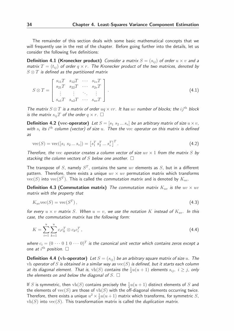
34 Chapter 4. Least-Squares Variance Component Estimation
The remainder of this section deals with some basic mathematical concepts that wewill frequently use in the rest of the chapter. Before going further into the details, let usconsider the following five definitions:
Definition 4.1 (Kronecker product) Consider a matrix S = (sij) of order u× v and amatrix T = (tij) of order q × r. The Kronecker product of the two matrices, denoted byS ⊗ T is defined as the partitioned matrix
S ⊗ T =
s11T s12T · · · s1vTs21T s22T · · · s2vT
......
. . ....
su1T su2T · · · suvT
. (4.1)
The matrix S⊗ T is a matrix of order uq× vr. It has uv number of blocks; the ijth blockis the matrix sijT of the order q × r. �
Definition 4.2 (vec-operator) Let S = [s1 s2 ... sv] be an arbitrary matrix of size u× v,with si its ith column (vector) of size u. Then the vec operator on this matrix is definedas
vec(S) = vec([s1 s2 ... sv]) =[sT1 sT
2 ... sTv
]T. (4.2)
Therefore, the vec operator creates a column vector of size uv × 1 from the matrix S bystacking the column vectors of S below one another. �
The transpose of S, namely ST , contains the same uv elements as S, but in a differentpattern. Therefore, there exists a unique uv × uv permutation matrix which transformsvec(S) into vec(ST ). This is called the commutation matrix and is denoted by Kuv.
Definition 4.3 (Commutation matrix) The commutation matrix Kuv is the uv × uvmatrix with the property that
Kuvvec(S) = vec(ST ) , (4.3)
for every u × v matrix S. When u = v, we use the notation K instead of Kuv. In thiscase, the commutation matrix has the following form:
K =u∑
i=1
u∑
k=1
cicTk ⊗ ckc
Ti , (4.4)
where ci = (0 · · · 0 1 0 · · · 0)T is the canonical unit vector which contains zeros except aone at ith position. �
Definition 4.4 (vh-operator) Let S = (sij) be an arbitrary square matrix of size u. Thevh operator of S is obtained in a similar way as vec(S) is defined, but it starts each columnat its diagonal element. That is, vh(S) contains the 1
2u(u + 1) elements sij, i ≥ j, only
the elements on and below the diagonal of S. �
If S is symmetric, then vh(S) contains precisely the 12u(u + 1) distinct elements of S and
the elements of vec(S) are those of vh(S) with the off-diagonal elements occurring twice.Therefore, there exists a unique u2× 1
2u(u+1) matrix which transforms, for symmetric S,
vh(S) into vec(S). This transformation matrix is called the duplication matrix.
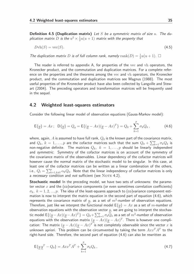
4.2 Weighted least-squares estimators 35
Definition 4.5 (Duplication matrix) Let S be a symmetric matrix of size u. The du-plication matrix D is the u2 × 1
2u(u + 1) matrix with the property that
Dvh(S) = vec(S). (4.5)
The duplication matrix D is of full column rank, namely rank(D) = 12u(u + 1). �
The reader is referred to appendix A, for properties of the vec and vh operators, theKronecker product, and the commutation and duplication matrices. For a complete refer-ence on the properties and the theorems among the vec and vh operators, the Kroneckerproduct, and the commutation and duplication matrices see Magnus (1988). The mostuseful properties of the Kronecker product have also been collected by Langville and Stew-art (2004). The preceding operators and transformation matrices will be frequently usedin the sequel.
4.2 Weighted least-squares estimators
Consider the following linear model of observation equations (Gauss-Markov model):
E{y} = Ax ; D{y} = Qy = E{(y − Ax)(y − Ax)T} = Q0 +
p∑
k=1
σkQk , (4.6)
where, again, A is assumed to have full rank, Q0 is the known part of the covariance matrix,and Qk, k = 1, . . . , p are the cofactor matrices such that the sum Q0 +
∑pk=1 σkQk is
non-negative definite. The matrices Qk, k = 1, . . . , p should be linearly independentand symmetric. Symmetry of the cofactor matrices is on account of the symmetry ofthe covariance matrix of the observables. Linear dependency of the cofactor matrices willhowever cause the normal matrix of the stochastic model to be singular. In this case, atleast one of the cofactor matrices can be written as a linear combination of the others,i.e., Ql =
∑pk=1,k 6=l αkQk. Note that the linear independency of cofactor matrices is only
a necessary condition and not sufficient (see Note 4.2).
Stochastic model In the preceding model, we have two sets of unknowns: the parame-ter vector x and the (co)variance components (or even sometimes correlation coefficients)σk, k = 1, 2, ..., p. The idea of the least-squares approach to (co)variance component esti-mation is now to interpret the matrix equation in the second part of equation (4.6), whichrepresents the covariance matrix of y, as a set of m2-number of observation equations.Therefore, just like we interpret the functional model E{y} = Ax as a set of m-number ofobservation equations with the observation vector y, we are going to interpret the stochas-
tic model E{(y−Ax)(y−Ax)T} = Q0+∑p
k=1 σkQk as a set of m2-number of observation
equations with the observation matrix (y − Ax)(y − Ax)T . There is however one compli-
cation: The matrix (y − Ax)(y − Ax)T is not completely observable since the vector x is
unknown apriori. This problem can be circumvented by taking the term AxxT AT to theright-hand side. Therefore, the second part of equation (4.6) can also be rewritten as
E{y yT −Q0} = AxxT AT +
p∑
k=1
σkQk , (4.7)
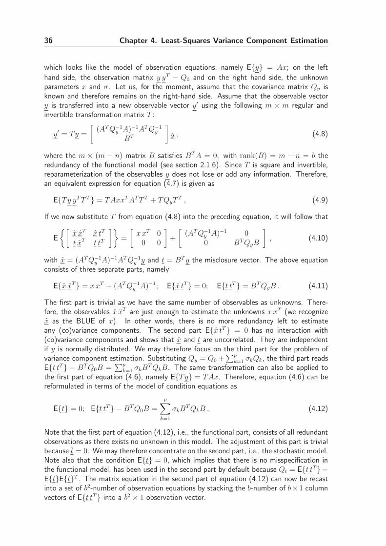
36 Chapter 4. Least-Squares Variance Component Estimation
which looks like the model of observation equations, namely E{y} = Ax; on the left
hand side, the observation matrix y yT − Q0 and on the right hand side, the unknownparameters x and σ. Let us, for the moment, assume that the covariance matrix Qy isknown and therefore remains on the right-hand side. Assume that the observable vectory is transferred into a new observable vector y′ using the following m × m regular andinvertible transformation matrix T :
y′ = Ty =
[(AT Q−1
y A)−1AT Q−1y
BT
]
y , (4.8)
where the m × (m − n) matrix B satisfies BT A = 0, with rank(B) = m − n = b theredundancy of the functional model (see section 2.1.6). Since T is square and invertible,reparameterization of the observables y does not lose or add any information. Therefore,an equivalent expression for equation (4.7) is given as
E{Ty yT T T} = TAxxT AT T T + TQyTT , (4.9)
If we now substitute T from equation (4.8) into the preceding equation, it will follow that
E
{[x xT x tT
t xT t tT
]}
=
[xxT 0
0 0
]
+
[(AT Q−1
y A)−1 00 BT QyB
]
, (4.10)
with x = (AT Q−1y A)−1AT Q−1
y y and t = BT y the misclosure vector. The above equationconsists of three separate parts, namely
E{x xT} = xxT + (AT Q−1y A)−1; E{x tT} = 0; E{t tT} = BT QyB . (4.11)
The first part is trivial as we have the same number of observables as unknowns. There-fore, the observables x xT are just enough to estimate the unknowns xxT (we recognizex as the BLUE of x). In other words, there is no more redundancy left to estimateany (co)variance components. The second part E{x tT} = 0 has no interaction with(co)variance components and shows that x and t are uncorrelated. They are independentif y is normally distributed. We may therefore focus on the third part for the problem ofvariance component estimation. Substituting Qy = Q0 +
∑pk=1 σkQk, the third part reads
E{t tT} − BT Q0B =∑p
k=1 σkBT QkB. The same transformation can also be applied to
the first part of equation (4.6), namely E{Ty} = TAx. Therefore, equation (4.6) can bereformulated in terms of the model of condition equations as
E{t} = 0; E{t tT} −BT Q0B =
p∑
k=1
σkBT QkB . (4.12)
Note that the first part of equation (4.12), i.e., the functional part, consists of all redundantobservations as there exists no unknown in this model. The adjustment of this part is trivialbecause t = 0. We may therefore concentrate on the second part, i.e., the stochastic model.Note also that the condition E{t} = 0, which implies that there is no misspecification inthe functional model, has been used in the second part by default because Qt = E{t tT}−E{t}E{t}T . The matrix equation in the second part of equation (4.12) can now be recastinto a set of b2-number of observation equations by stacking the b-number of b×1 columnvectors of E{t tT} into a b2 × 1 observation vector.
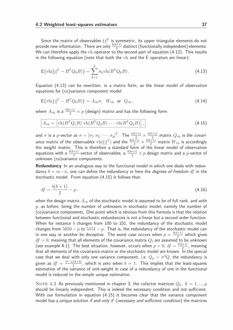
4.2 Weighted least-squares estimators 37
Since the matrix of observables t tT is symmetric, its upper triangular elements do notprovide new information. There are only b(b+1)
2distinct (functionally independent) elements.
We can therefore apply the vh operator to the second part of equation (4.12). This resultsin the following equation (note that both the vh and the E operators are linear):
E{vh(t tT −BT Q0B)} =
p∑
k=1
σkvh(BT QkB) . (4.13)
Equation (4.13) can be rewritten, in a matrix form, as the linear model of observationequations for (co)variance component model:
E{vh(t tT −BT Q0B)} = Avhσ, Wvh or Qvh , (4.14)
where Avh is a b(b+1)2× p (design) matrix and has the following form:
Avh =[vh(BT Q1B) vh(BT Q2B) · · · vh(BT QpB)
], (4.15)
and σ is a p-vector as σ = [σ1 σ2 · · · σp]T . The b(b+1)
2× b(b+1)
2matrix Qvh is the covari-
ance matrix of the observables vh(t tT ) and the b(b+1)2× b(b+1)
2matrix Wvh is accordingly
the weight matrix. This is therefore a standard form of the linear model of observationequations with a b(b+1)
2-vector of observables, a b(b+1)
2× p design matrix and a p-vector of
unknown (co)variance components.
Redundancy In an analogous way to the functional model in which one deals with redun-dancy b = m−n, one can define the redundancy or here the degrees of freedom df in thestochastic model. From equation (4.15) it follows that:
df =b(b + 1)
2− p , (4.16)
when the design matrix Avh of the stochastic model is assumed to be of full rank, and withp, as before, being the number of unknowns in stochastic model, namely the number of(co)variance components. One point which is obvious from this formula is that the relationbetween functional and stochastic redundancies is not a linear but a second order function.When for instance b changes from 100 to 101, the redundancy of the stochastic modelchanges from 5050− p to 5151− p. That is, the redundancy of the stochastic model canin one way or another be deceptive. The worst case occurs when p = b(b+1)
2which gives
df = 0, meaning that all elements of the covariance matrix Qt are assumed to be unknown(see example 4.1). The best situation, however, occurs when p = 0, df = b(b+1)
2, meaning
that all elements of the covariance matrix or the stochastic model are known. In the specialcase that we deal with only one variance component, i.e. Qy = σ2Q, the redundancy is
given as df = (b−1)(b+2)2
, which is zero when b = 1. This implies that the least-squaresestimation of the variance of unit-weight in case of a redundancy of one in the functionalmodel is reduced to the simple unique estimation.
Note 4.2 As previously mentioned in chapter 3, the cofactor matrices Qk, k = 1, ..., pshould be linearly independent. This is indeed the necessary condition and not sufficient.With our formulation in equation (4.15) it becomes clear that the variance componentmodel has a unique solution if and only if (necessary and sufficient condition) the matrices
38 Chapter 4. Least-Squares Variance Component Estimation
BT QkB, k = 1, ..., p are linearly independent. From the definition of the redundancy dfof the stochastic model it goes without saying that the maximum number of estimable(co)variance components in the stochastic model is b(b+1)
2which leads to df = 0 (unique
solution). That is, in general an m(m+1)2− b(b+1)
2number of distinct elements of Qy remains
inestimable as m ≥ b. Xu et al. (2007) also prove that all variance and covariances are
not estimable. They propose a method to show that at most only a b(b+1)2
number ofindependent parameters are estimable. ⊡
(Co)variance estimators (1) Having established these results, we can now apply theestimation methods of chapter 2. That is, if the weight matrix Wvh is known (or assumed),we can obtain the weighted (deterministic) least-squares estimators of the (co)variancecomponents. The weighted least-squares estimators of the (co)variance components thenread (cf. equation (2.6))
σ = (ATvhWvhAvh)
−1ATvhWvhvh(t tT −BT Q0B) . (4.17)
If we denote N = ATvhWvhAvh and l = AT
vhWvhvh(t tT−BT Q0B) it follows that σ = N−1l.This equation can be written out in full as
σ1
σ2...
σp
=
n11 n12 · · · n1p
n12 n22 · · · n2p...
.... . .
...n1p n2p · · · npp
−1
l1l2...lp
, (4.18)
where
nkl = vh(BT QkB)T Wvhvh(BT QlB) , (4.19)
and
lk = vh(BT QkB)T Wvhvh(t tT−BT Q0B) , (4.20)
with k, l = 1, 2, · · · , p. Any symmetric and positive-definite matrix Wvh can play the roleof the weight matrix. An important feature of the preceding estimators is the unbiasednessproperty. One can obtain the BLUE estimators (or in fact BIQUE estimators as they resultsin a quadratic form of the original observables) by taking the weight matrix as the inverseof Qvh. Unfortunately, in practice it is not always possible to obtain Qvh as it dependson the fourth central moments of the observables (see equation (4.53)) which may not beobtainable all the times, but only for special cases. In the following, we will however showtwo examples as limiting cases that no supposition on the distribution is required.
Example 4.1 Consider the model of condition equations E{BT y} = E{t} = 0 with a completelyunknown covariance matrix Qt (all elements are unknown). It is possible to obtain the solutionof these unknown (co)variance components. For this purpose we can write the unknown matrixQt as
Qt =
b(b+1)2∑
k=1
σkCk, with Ck =
cicTj , if σk = σii, i = j ,
cicTj + cjc
Ti , if σk = σij , i 6= j ,
(4.21)
4.2 Weighted least-squares estimators 39
where σk is respectively σ11, σ12, ..., σ1b, σ22, σ23, ..., σbb and ci = (0 · · · 1 · · · 0)T is the canonicalunit vector of size b containing zeros except a one at ith position. With the preceding formulation,the matrices BT QkB in equation (4.15) are of the form Ck = cic
Ti or Ck = cic
Tj + cjc
Ti .
Applying the vh operator to these matrices gives canonical unit vectors in Rb(b+1)
2 . That is, Avh
in equation (4.14) is given as Avh = I b(b+1)2
. This means that the (co)variance components σ
can be uniquely estimated as
σ = vh(Qt) = A−1
vh vh(t tT ) = vh(t tT ) , (4.22)
which is independent of the weight matrix Wvh or covariance matrix Qvh, and therefore ofdistribution of t. This expression can be rewritten as Q
t= t tT . One can also obtain the
covariance matrix of these estimators (see example 4.4). �
Example 4.2 If we measure a zero-mean quantity (see Note 4.1), then E{BT y} = E{y} =E{t} = 0, b = m. Let the observables be independent and identically distributed (in generalunknown distribution). In this case Qt = σ2I with σ2 an unknown variance component to beestimated. It is not difficult to show that only the following central moments (up to degree four)are non-zero
E{t2i } = µ2; E{t4i } = µ4; E{t2i t2j} =
µ4 if i = j ,
µ22 if i 6= j .
(4.23)
With these non-zero elements it becomes clear that Qvh is diagonal with the entries
diag(Qvh) = (µ4 − µ22 ,
m−1 times︷ ︸︸ ︷
µ22 , ... , µ2
2 , µ4 − µ22 ,
m−2 times︷ ︸︸ ︷
µ22 , ... , µ2
2 , ... , ... , µ4 − µ22). (4.24)
After a few simple mathematical operations one obtains the inverse of the matrix Qvh as
Q−1vh =
1
µ4 − µ22
DT (I ⊗ I)D +µ4 − 3µ2
2
µ22(µ4 − µ2
2)(DT D − Im(m+1)
2
). (4.25)
In equation (4.17) we have Avh = vh(I). If observables are normally distributed, then µ4 = 3σ4
and therefore the second term of Q−1vh vanishes. But even though the distribution is not specified,
the second term when pre-multiplied with vh(I)T becomes zero. Therefore, one obtains
N = n11 =m
µ4 − µ22
; l = l1 =tT t
µ4 − µ22
, (4.26)
which gives the variance estimator σ2 independent of µ4 as
σ2 =tT t
m. (4.27)
This estimator is therefore independent of the unspecified distribution of t. Such an estimator isnot only unbiased but also of minimum variance. Note however that the variance of this estimatoris given as N−1 = n−1
11 which is obtainable when we specify the distribution. �
40 Chapter 4. Least-Squares Variance Component Estimation
Weight matrix As mentioned, any symmetric and positive-definite matrix Wvh can playthe role of weight matrix in equation (4.17). From a numerical point of view such arbitraryweight matrices may not be advisable as they are as large as by the second power of thesample size. Now we will restrict ourselves to those weight matrices which computationallyare more efficient. To find different classes of admissible weight matrices Wvh we firstcome up with different classes of admissible weight matrices for Wvec. Pre-multiplyingequation (4.14) with the duplication matrix D yields that
E{vec(t tT −BT Q0B)} = DAvhσ, Wvec . (4.28)
We now recall the property of invariance of the estimators under a regular transformationmatrix T . Let us assume that the original observation vector t is transformed into v usingthe non-singular b× b matrix M , i.e. v = M t or t = M−1v. In this case, one obtains
vec(t tT ) = vec(M−1v vT M−T ) . (4.29)
Using equation (A.13), in appendix A, the preceding equation reads
vec(t tT ) = (M−1 ⊗M−1)vec(v vT ) = Tvec(v vT ) . (4.30)
To make our estimators independent of the type of reparameterization of observables, wecan use the identity W t
vec = T−T W vvecT
−1, which yields
W tvec = (MT ⊗MT )W v
vec(M ⊗M) . (4.31)
From the definition of vec and vh operators, it follows that for any symmetric matrixone gets vec = DD+vec where D+ is the pseudo inverse (Moore-Penrose inverse) of thematrix D and is given as D+ = (DT D)−1DT (see appendix A). Since the matrix DD+ has
rank b(b+1)2
, this implies that we will only deal with b(b+1)2
number of distinct (functionallyindependent) elements. Therefore, in order to specify a class of weight matrices for the vhoperator, we can argue that both the vec and vh operators should give identical estimators.Comparing the least-squares solution of equation (4.14) with that of equation (4.28) simplywith equation (4.31) follows that
Wvh = DT WvecD = DT (MT ⊗MT )W vvec(M ⊗M)D . (4.32)
In order for the weight matrix Wvh to be simple, we may take simple forms for W vvec in the
preceding equation. Here we consider two choices as follows:
• The identity matrix W vvec = Ib2 = I ⊗ I is positive-definite and therefore an element
of this class. It follows then
Wvh = DT (MT ⊗MT )I(M ⊗M)D = DT (MT M ⊗MT M)D . (4.33)
Since MT M is a positive-definite symmetric matrix, a class of admissible weightmatrices for vh(t tT ) is given as
Wvh = DT (Wt ⊗Wt)D , (4.34)
where Wt is an arbitrary positive-definite symmetric matrix. Using the properties ofthe Kronecker product one can show that Wvh is also positive-definite and thereforecan play the role of the weight matrix.
4.2 Weighted least-squares estimators 41
• The second weight matrix includes, in addition to identity matrix, one more simpleterm as W v
vec = I ⊗ I +αvec(I)vec(I)T . For some α, namely α > −1b
, this matrix ispositive-definite. When substituted in equation (4.33), the second term simplifies to(see equation (A.13)): (MT ⊗MT )(vec(I)vec(I)T )(M ⊗M) = vec(Wt)vec(Wt)
T .This results in the following weight matrix:
Wvh = DT (Wt ⊗Wt + α vec(Wt)vec(Wt)T )D . (4.35)
(Co)variance estimators (2) In this thesis we consider only the simplest weight matrixWvh = DT (Wt ⊗Wt)D (first choice). But we will as well give a few comments on thesecond case. Equation (4.14) can therefore be rewritten as
E{vh(t tT −BT Q0B)} = Avhσ, Wvh = DT (Wt ⊗Wt)D, (4.36)
with Wt any positive-definite symmetric matrix and D the duplication matrix. Substitutionof vh with D+vec and Wvh = DT (Wt ⊗Wt)D in equation (4.19) follows
nkl = vec(BT QkB)T D+T DT (Wt ⊗Wt)DD+vec(BT QlB) . (4.37)
Using identities (A.21) and (A.22) with (A.15) and (A.18), in appendix A, the termsD+T DT and DD+ in the preceding equation can be left out, i.e.
nkl = vec(BT QkB)T (Wt ⊗Wt)vec(BT QlB) . (4.38)
This also confirms that the operators vh and vec, on symmetric matrices, give identicalresults. Using equation (A.14), the preceding equation reads
nkl = tr(BT QkBWtBT QlBWt). (4.39)
In a similar manner, lk of equation (4.20) simplifies
lk = tr(BT QkBWt[t tT −BT Q0B]Wt) (4.40)
or finally
lk = tT WtBT QkBWtt− tr(BT QkBWtB
T Q0BWt). (4.41)
The weighted least-squares (co)variance component estimation was formulated byrewriting the (co)variance component model into a linear model of observation equations.Note that the above formulation to (co)variance component estimation is based on the de-terministic least-squares technique for which an arbitrary weight matrix Wvh (e.g. in formof equation (4.34)) can be used. The (co)variance components are therefore estimated asa linear unbiased estimator (LUE) of the quadratic misclosures vh(t tT ) which can then berewritten as an invariant quadratic unbiased estimator (IQUE) of the misclosures t.
The following example shows that the empirical autocovariance function is a weightedLS-VCE, if the weight matrix is chosen from the given weight matrix class in equa-tion (4.34).
42 Chapter 4. Least-Squares Variance Component Estimation
Example 4.3 (unbiased empirical autocorrelation function) Let yi, i = 1, . . ., be a zero-mean stationary random process, with unknown covariance function σij = στ (τ = |i− j|). If mrandom variables are available, we have, with y = (y
1, . . . , y
m)T , that
E{y} = 0 and D{y} = Qy =m−1∑
τ=0
στQτ , (4.42)
with the m×m cofactor matrices
Qτ = aτ
m−τ∑
i=1
(cicTi+τ + ci+τc
Ti ) , (4.43)
for τ = 0, 1, . . . , m − 1, with a0 = 12 and aτ = 1 for τ 6= 0. Note that σ0 is the variance of yi
and that στ is the covariance between yi and yi+τ .We can now apply the above formulation to estimate σ = (σ0, σ1, . . . , σm−1)
T . In our casewe have t = BT y, with B = I. We will use Wt = Wy = I as weight matrix. Substitution ofB = I and Wt = Wy = I into equation (4.39), gives, with equation (4.43) (see below)
nτ,κ = tr(QτQκ) =
{2aτ (m− τ) if τ = κ ;0 if τ 6= κ .
(4.44)
Therefore, the normal matrix is a diagonal matrix. In a similar manner, and with Q0 = 0, we findfor the entries of the right-hand side vector, lτ = 2aτ
∑m−τi=1 y
iy
i+τ(see below). The LS-VCE
solution for the unknown (co)variance components follows therefore as
στ =
∑m−τi=1 y
iy
i+τ
m− τ, τ = 0, 1, . . . , m− 1. (4.45)
This solution is known as the unbiased sample autocovariance function of a zero-mean stationarytime-series yi, see e.g. Priestley (1981). We thus have shown that the sample autocovariancefunction is a LS-VCE, if the weight matrix is chosen as the identity matrix. If one has a functionallyknown quantity with mean µ, one will use the residuals ei = y
i−µ in the preceding formula. One
can also compute the correlation coefficients that together represent the empirical autocorrelationfunction (ACF)
ρτ
=στ
σ0
, τ = 1, ..., m− 1. (4.46)
where σ0 = σ2 is the variance of the noise process, and στ the covariances. �
Proof. (nτ,κ and lτ
) Substitution of Qτ = aτ∑m−τ
i=1 (cicTi+τ + ci+τc
Ti ) and Qκ =
aκ∑m−κ
j=1 (cjcTj+κ + cj+κcT
j ) into nτ,κ = tr(QτQκ) results in the following equation
nτκ = 2aτaκ
m−τ∑
i=1
m−κ∑
j=1
tr(cicTi+τcjc
Tj+κ + cic
Ti+τcj+κcT
j ), (4.47)
or
nτκ = 2aτaκ
m−τ∑
i=1
m−κ∑
j=1
δi+τ,jδi,j+κ + δi+τ,j+κδi,j , (4.48)
4.3 Covariance matrix of observables vh(t tT ) 43
where δi,j is the Kronecker delta. The first term of the above equation is identical to zero exceptfor the case that τ = κ = 0. Also, the second term is zero when τ 6= κ. It then follows thatnτ,τ = 2aτ (m − τ) and nτ,κ = 0 if τ 6= κ. For the right-hand side vector, substitution ofQτ = aτ
∑m−τi=1 (cic
Ti+τ + ci+τc
Ti ) in lτ = yT Qτy gives
lτ = aτ
m−τ∑
i=0
yT cicTi+τy + yT ci+τc
Ti y, (4.49)
or, finally
lτ = 2aτ
m−τ∑
i=0
yiy
i+τ. H (4.50)
Before we enumerate the attractive features of the least-squares approach to (co)variancecomponent estimation, let us first derive the covariance matrix of the observables vh(t tT ).
4.3 Covariance matrix of observables vh(t tT )
In order to evaluate the covariance matrix of (co)variance components, i.e. Qσ, we need
to know the b(b+1)2× b(b+1)
2covariance matrix of vh(t tT ), namely Qvh. In addition, one
can in particular take the weight matrix Wvh to be the inverse of Qvh to obtain the BLUEestimators (or better say BIQUE estimators, as our ’observations’ are in quadratic form ofthe original ones). Let us first derive the covariance matrix of vec(t tT ) which is based onthe following theorem:
Theorem 4.1 (Central moments) Let the stochastic vector t be normally distributedwith mean zero and covariance matrix Qt, i.e. t ∼ N(0, Qt), then the odd-order centralmoments of t are zero, and the second and fourth central moments are of the form
E{titj} = qij ;E{titjtktl} = qijqkl + qikqjl + qjkqil ;i, j, k, l = 1, 2, · · · , b ,
(4.51)
where qij represents Qt in index notation, i.e., qij = Qti,tj . ⊠
Proof. For a proof of the preceding theorem we refer to appendix C. H
Note 4.3 The multivariate normal distribution is classified as an elliptical distribution.Another example of elliptical distributions is the multivariate Student t distribution. Forelliptically contoured distributed data one needs to define a kurtosis parameter κ in orderto obtain the moments of different orders, see Berkane and Bentler (1986); Maruyama andSeo (2003); Teunissen and Amiri-Simkooei (2006). The kurtosis parameter for normallydistributed data is zero. ⊡
Covariance matrix Qvec The elements of the covariance matrix Qvec are by definitiongiven as
Qi j k lvec = E{(titj − E{titj})(tktl − E{tktl})}, i, j, k, l = 1, 2, · · · , b . (4.52)
44 Chapter 4. Least-Squares Variance Component Estimation
This shows the covariance between elements of observable vector vec(t tT ), i.e. betweentitj and tktl. If we factor the right-hand side we obtain
Qi j k lvec = E{titjtktl} − E{titj}E{tktl}, i, j, k, l = 1, 2, · · · , b . (4.53)
This result shows that we need the second and the fourth multivariate central moments ofthe random vector t. Using Theorem 4.1, equation (4.53) as a fourth-order tensor, can bewritten as
Qijklvec = C{titj, tktl} = qikqjl + qjkqil, i, j, k, l = 1, 2, ..., b . (4.54)
One can rewrite the preceding equation in terms of a second-order tensor (a matrix). Tofollow consider the following theorem:
Theorem 4.2 Let Qt = qij be a symmetric and positive-definite matrix of size b. ThenQijkl
vec = qikqjl + qjkqil, i, j, k, l = 1, 2, ..., b, as a fourth-order tensor, is equivalent to thefollowing second-order tensor (matrix):
Qvec = 2 DD+(Qt ⊗Qt)D+T DT , (4.55)
which represents the covariance matrix of the observable vector vec(t tT ), where the b2 ×b(b+1)
2matrix D is the duplication matrix. ⊠
Proof. From Qijklvec = qikqjl + qjkqil, i, j, k, l = 1, 2, ..., b it follows that the b2 × b2 covariance
matrix Qvec, as a fourth order tensor, is composed of b2-number of b× b submatrices, i.e.
Qvec =
Q1.1. Q1.2. · · · Q1.b.
Q2.1. Q2.2. · · · Q2.b.
...... Qi.k.
...Qb.1. Qb.2. · · · Qb.b.
, (4.56)
where the b×b submatrix Qi.k. is of the form Qi.k. = cTi QtckQt+Qtckc
Ti Qt, with ci the canonical
unit vector. Equation (4.56) can be rewritten as follows:
Qvec =b∑
i=1
b∑
k=1
cicTk ⊗Qi.k.. (4.57)
Substituting Qi.k. = cTi QtckQt + Qtckc
Ti Qt in the preceding equation yields (note that the term
cTi Qtck = qik is a scalar)
Qvec =b∑
i=1
b∑
k=1
cTi Qtckcic
Tk ⊗Qt + cic
Tk ⊗Qtckc
Ti Qt. (4.58)
Using the properties of the Kronecker product, after a few simple matrix operations, the precedingequation yields
Qvec = [Qt ⊗Qt + (I ⊗Qt)K(I ⊗Qt)], with K =b∑
i=1
b∑
k=1
cick ⊗ ckcTi , (4.59)
the commutation matrix (see definition 4.3). Using equation (A.24) and then equations (A.5)and (A.27), the preceding equation reads
Qvec = [I + K](Qt ⊗Qt) = 2DD+(Qt ⊗Qt), (4.60)
which with equations (A.22) and (A.18) completes the proof. H
4.4 Properties of least-squares estimators 45
Covariance matrix Qvh One can show that the covariance matrix Qvec suffers from a rankdeficiency of b(b−1)
2. This is what we would expect. The b(b−1)
2number of elements of matrix
t tT located in the upper triangle do not introduce new information. That is why they areone-to-one correlated with those located in the lower triangle. This causes the matrix Qvec
to be rank deficient. Applying the error propagation law to vh(t tT ) = D+vec(t tT ) resultsin the covariance matrix of the observable vector vh(t tT )
Qvh = 2 D+(Qt ⊗Qt)D+T , (4.61)
which is a symmetric and positive-definite matrix provided that Qt is positive-definite;rank(Qvh) = b(b+1)
2. Using the properties of the duplication matrix, the inverse of Qvh is
obtained as (see identity (A.23))
Q−1vh =
1
2DT (Q−1
t ⊗Q−1t )D . (4.62)
Note 4.4 For normally distributed data, Q−1vh is an element of the class of admissible
weight matrices defined in equation (4.34) with
Wt =1√2Q−1
t . (4.63)
Teunissen and Amiri-Simkooei (2006) show that for elliptically contoured distributed data,the inverse of Qvh is of the form
Q−1vh =
1
2(κ + 1)DT
[
Q−1t ⊗Q−1
t −κ
2(κ + 1) + κbvec(Q−1
t )vec(Q−1t )T
]
D . (4.64)
This means that for elliptical distributions the above matrix is an element of the weightmatrix defined in equation (4.35) with
Wt =1
√
2(κ + 1)Q−1
t ; and α =−κ
2(κ + 1) + κb. (4.65)
This is in fact an interesting result because we can now take the weight matrix as Wvh =Q−1
vh to obtain the minimum variance estimators of the (co)variance components (notonly for the normal distribution but also for a larger class of elliptical distributions, seesection 4.5). ⊡
4.4 Properties of least-squares estimators
4.4.1 Optimal properties
The above (weighted) least-squares solutions to the (co)variance components are inde-pendent of the distribution of vh(t tT ) which has been left unspecified so far. Since theapproach is based on the least-squares principle, we know without any additional derivationthat the estimators are unbiased . This property is also independent of the distribution (oreven the covariance matrix) of the observable vector vh(t tT ).
Note that the weighted least-squares solution is however not necessarily of minimumvariance as we can use any positive-definite symmetric matrix as the weight matrix in
46 Chapter 4. Least-Squares Variance Component Estimation
equation (4.34). This problem can however be circumvented by taking the weight matrixto be the inverse of the covariance matrix, i.e. Wvh = Q−1
vh (see next section). Therefore, inthis alternative and indeed the most efficient technique, we can use the ’probabilistic’ least-squares technique to obtain the BLUE estimators (or better say, BIQUE estimators, sincethe observables are in quadratic form of the original ones, i.e. vh(t tT )) of the (co)variancecomponents. In the previous section, we specified the covariance matrix Qvh for thenormal distribution. Therefore, in this thesis, the property of minimum variance of the(co)variance component estimators is restricted to the class of normally distributed data.As a generalization, Teunissen and Amiri-Simkooei (2006) give the minimum varianceestimators for a larger class of distributions, namely elliptical distributions.
4.4.2 Covariance matrix of estimators
Since the (weighted) least-squares estimators are in a linear form of the observables vh(t tT ),applying the error propagation law to equation (4.17) automatically gives us the covariancematrix of the estimated (co)variance components, namely Qσ, provided that the properQvh, or equivalently the proper Qt, is input as the covariance matrix of the vector vh(t tT ).Applying the error propagation law to equation (4.17) gives (cf. equation (2.9))
Qσ = N−1ATvhWvhQvhWvhAvhN
−1 , (4.66)
or simply
Qσ = N−1MN−1, (4.67)
where the p× p matrix M is given as
M = ATvhWvhQvhWvhAvh . (4.68)
It is also possible to simplify the preceding equation. Substituting for Wvh from equa-tion (4.34) and for Qvh from equation (4.61) gives
mkl = 2tr(BT QkBWtQtWtBT QlBWtQtWt), (4.69)
where mkl represents the p× p matrix M in index notation.
Proof. Matrix M is given as M = ATvhWvhQvhWvhAvh = mkl =
vh(BT QkB)T WvhQvhWvhvh(BT QlB) where Wvh = DT (Wt ⊗ Wt)D and for normaldistribution Qvh = 2D+(Qt ⊗ Qt)D
+T . Substitution of these terms, with vh(.) = D+vec(.)and DD+vec(.) = vec(.), gives the above expression for M . H
Equation (4.67) can therefore provide us with the precision of the estimators. This is infact an important feature of the least-squares variance component estimation. Since thecovariance matrix Qvh depends on the distribution of the original observations, our resultsare again restricted to the class of normal distributions.
Example 4.4 (Example 4.1 continued) Let us assume that the misclosures t are normally dis-tributed. It is now possible to compute the covariance matrix of the estimated (co)varianceelements of Qt, namely the covariance matrix of σ = vh(Q
t) = A−1
vh vh(t tT ) = vh(t tT ). This is
4.4 Properties of least-squares estimators 47
in fact a very simple example as Avh = I. Application of the error propagation law to σ = vh(t tT )gives
Qσ = Qvh = 2D+(Qt ⊗Qt)D+T . (4.70)
In the preceding equation Qt is unknown apriori. One will thus have to be satisfied with anestimate of Qt, namely Qt = t tT . This leads to an estimate of Qσ as
Qσ = 2D+(t tT ⊗ t tT )D+T . (4.71)
Strictly speaking, the (co)variance elements of Qt are estimated as σij = ti tj , with the varianceof σ2
σij= 2t2i t2j (follow similar way to Theorem 4.2 when k = i and l = j). Note that the
estimator σij is of the same order as its standard deviation σσij. This indicates that the estimated
(co)variance elements σij may not be precise enough. In practice one may not have all the
elements of Qt to be unknown but only p << b(b+1)2 (co)variance components which leads to a
better precision of their related estimators. In the sequel, just for the sake of convenience, wewill drop the hat notation located on top and simply denote Q as Q. �
Example 4.5 (Example 4.3 continued ) To determine the precision of the empirical autoco-variance function, we will assume that y is normally distributed. The entries of matrix N inthe expression of the covariance matrix Qσ = N−1MN−1 of σ = (σ0, . . . , σm−1)
T , are given inequation (4.44). To determine the entries of matrix M , we substitute Wt = Wy = I and B = Iinto equation (4.69). This gives
mτκ = 2tr(QτQyQκQy). (4.72)
Therefore, the entries of the covariance matrix are given as
(Qσ)τκ =tr(QτQyQκQy)
2a2τ (m− τ)2
. (4.73)
This expression is easily evaluated numerically. A simple, but approximate, analytical expressioncan be obtained, if we approximate the covariance matrix of y by Qy ≈ σ0I. This is a goodapproximation, the closer the randomness of the time-series resembles that of white noise. Withthis approximation, the covariance matrix of equation (4.73) becomes a diagonal matrix, withentries
σ2στ
=σ4
aτ (m− τ), τ = 0, 1, ..., m− 1, (4.74)
with σ4 = σ20. To obtain the variance of the autocorrelation function one can apply the error
propagation law to the linearized form of equation (4.46)
σ2ρτ
=1
m− τ+
2ρ2τ
m, τ = 1, ..., m− 1. (4.75)
This shows that the precision of the autocorrelation function gets poorer with increasing time-lagτ . This also makes sense, since less data are used when τ increases. �
4.4.3 Quadratic form of residuals
Since the approach is based on the least-squares principle, parts of the standard qualitycontrol theory can be applied to the model in equation (4.36) and the result in equa-tion (4.18). One can in particular apply the idea of hypotheses testing to the stochastic
48 Chapter 4. Least-Squares Variance Component Estimation
model. Chapter 5 deals with the w-test statistic and the quadratic form of the residuals inthe stochastic model.
As an important measure of any least-squares solution, one can compute the quadraticform of the residuals. This quadratic form is given by equation (2.11) for the functionalmodel. This can in fact be generalized for the least-squares (co)variance component esti-mation, i.e. to the stochastic model. Therefore, one will obtain
eTvhWvhevh = vh(t tT −BT Q0B)T [Wvh −WvhAvhN
−1ATvhWvh]vh(t tT −BT Q0B) .
(4.76)
In a similar manner to the previous derivations, substitution Wvh = DT (Wt⊗Wt)D resultsin the following formula:
eTvhWvhevh =(tT Wtt)
2 − 2tT WtBT Q0BWtt + tr(BT Q0BWtB
T Q0BWt)− lT N−1l ,
(4.77)
with N and l introduced in equations (4.39) and (4.41), respectively. If Q0 = 0, then itfollows that
eTvhWvhevh = (tT Wtt)
2 − lT N−1l , (4.78)
with lk = tT WtBT QkBWtt obtained from equation (4.41). Note that the quadratic form
is also independent of the (unspecified) distribution of the observable vector vh(t tT ).
4.4.4 Prior information
In some cases, we may have prior information about the (co)variance components. Suchinformation can be provided by equipment manufacturers or from a previous process. Letus assume that this information can be expressed as σ0 in the following way
E{σ0} = Cσ ; Wσ0 , (4.79)
where Wσ0 is the weight matrix of σ0 and C is a known matrix. One important featureof the LS-VCE is the possibility of incorporating such prior information with the observ-ables vh(t tT ). Without additional derivations, we can obtain the weighted least-squares(co)variance estimators as (Teunissen, 2000a)
σ = N−1l + N−1CT (CN−1CT + W−1σ0
)(σ0 − CN−1l). (4.80)
The method uses all of the information in an optimal way. Concerning the precedingformulation, we can at least mention that
• the method is considered as a competitor to the Bayesian method. The prior infor-mation, here for the LS-VCE, is in the form of the weight or covariance matrix ratherthan the probability density function,
• the method can be used as a regularization technique for ill-posed (co)variance com-ponent models (see ill-posed problems in section 4.8.3),
4.5 Minimum variance estimators 49
• the method may also be used for incorporating several estimators obtained fromvarious data sets in a sequential way.
• if we choose W−1σ0
= 0, then the solution obtained corresponds to using the hardconstraints σ0 = Cσ.
• if we choose Wvh = Q−1vh and Wσ0 = Q−1
σ0, we then obtain the minimum variance
estimators. In this case, the covariance matrix of estimators is simply given asQσ = (N + CT Q−1
σ0C)−1 = N−1 −N−1CT (CN−1CT + Qσ0)
−1CN−1 (cf. later onequation (4.88)),
4.4.5 Robust estimation
Since we estimated the (co)variance components on the basis of a linear model of obser-vation equations (see equation (4.36)), we can think of robust estimation methods ratherthan the least-squares. One can in particular think of an L1 norm minimization problem.The usual method for implementation of the L1 norm adjustment leads to the solving of alinear programming problem. For more information we refer to e.g. Amiri-Simkooei (2003).This may be an important alternative if one wants to be guarded against misspecificationsin the functional part of the model.
Example 4.6 In example 4.2 we can apply the idea of L1 norm minimization problem. Thestochastic model expressed in terms of a model of observation equations is as follows:
E{vh(t tT )} = vh(I)σ2, Wvh = I . (4.81)
The L1 norm principle states that the sum of the absolute values of the ’residual’ vector vh(t tT )−vh(I)σ2 should be minimized. Because b(b−1)
2 elements of vh(I) are zeros, they do not effect theminimization problem. Therefore, the L1 norm minimization problem is reduced to the followingproblem:
m∑
i=1
|t2i − σ2| → min . (4.82)
This is in fact very similar to the problem of measuring one unknown quantity, where the observ-ables are t2i , i = 1, ..., m. It is well known that the L1 norm minimization will lead to the samplemedian as an estimator of the population mean for repeated measurements of an unknown quan-tity. Therefore, the variance component is estimated as the median of the t21, t
22, ..., t
2m, namely
σ2 = t2m+12
, (4.83)
whereas the least-squares solution gives the mean of t21, t22, ..., t
2m (see example 4.2). �
4.5 Minimum variance estimators
As with the BLUE estimator introduced in chapter 2, the (co)variance components canbe estimated as the best linear unbiased estimator of the observables vh(t tT ). One canobtain such estimators by taking the weight matrix Wvh as the inverse of the covariancematrix of the observables, Q−1
vh . Then this linear form of the observables vh(t tT ) can bewritten as the best (minimum variance) quadratic unbiased estimator of the misclosures
50 Chapter 4. Least-Squares Variance Component Estimation
t. This can therefore be considered as an alternative derivation of the BIQUE estimatorintroduced in chapter 3. In section 4.3 we derived the covariance matrix Qvh for normallydistributed data. Therefore, the ’best’ (minimum variance) property is restricted to thenormal distribution (or even to a larger class of elliptical distributions).
Estimator To obtain the minimum variance estimators, one needs to substitute Wvh =Q−1
vh = 12DT (Q−1
t ⊗Q−1t )D in equation (4.17)
σ = N−1l = (ATvhQ
−1vh Avh)
−1ATvhQ
−1vh vh(t tT −BT Q0B) . (4.84)
After simplification, the p× p normal matrix N , and the p× 1 vector l read, respectively(follow the same way as the previous derivations)
nkl =1
2tr(BT QkBQ−1
t BT QlBQ−1t ), (4.85)
and
lk =1
2tT Q−1
t BT QkBQ−1t t− 1
2tr(BT QkBQ−1
t BT Q0BQ−1t ). (4.86)
Note that the preceding equations can simply be obtained from equations (4.39) and (4.41)with Wt = 1√
2Q−1
t (see equation (4.63)). In the case that Q0 = 0, the preceding equation
reads
lk =1
2tT Q−1
t BT QkBQ−1t t . (4.87)
Note 4.5 For elliptically contoured distributed data one can obtain the above estimatorsby choosing the inverse of covariance matrix Qvh given in equation (4.64) as the weightmatrix. The normal matrix N and the vector l are respectively given as (follow the sameway as the previous derivations)
nkl = 12(κ+1)
[tr(BT QkBQ−1t BT QlBQ−1
t )+αtr(BT QkBQ−1t )tr(BT QlBQ−1
t )];
lk = 12(κ+1)
[tT Q−1t BT QkBQ−1
t t + α(tT Q−1t t)tr(BT QkBQ−1
t )],
with κ the kurtosis parameter and α defined in equation (4.65). Note again that for normaldistribution κ = α = 0. ⊡
Covariance matrix Since we have formulated our variance component estimation problemin the least-squares sense, we know without any additional derivation that the inverse of thenormal matrix N automatically gives us the covariance matrix of the estimated (co)variancecomponents
Qσ = N−1, (4.88)
which provides us with the precision of the (co)variance estimators. The preceding equationcan also be obtained from equation (4.67) because in this case M = N .
4.5 Minimum variance estimators 51
Implementation of LS-VCE (B model)
Input:1. matrix B of condition equations;2. observation vector y;3. cofactor matrices Qk, k = 0, ..., p ;4. initial (co)variance components σ = σ0 = [σ0
1, ..., σ0p]
T ;5. small value for ǫ;
begincheck for presence of gross errors in observations;compute misclosures t = BT y;set iteration counter i = 0;begin
evaluate matrix Qy = Q0 +∑p
k=1 σkQk;compute matrix Qt = BT QyB;invert covariance matrix Qt;calculate matrix N and vector l from equations (4.85) and (4.86);solve for a new σ from normal equations Nσ = l;increase i by one step;update vector σi ← σ;while ‖σi − σi−1‖Q−1
σ> ǫ repeat;
end
obtain σ and its covariance matrix Qσ = N−1.end
Figure 4.1: Symbolic algorithm for implementation of least-squares variance component estimation
in terms of linear model of condition equations (B-model); σi contains the (co)variance components
estimated in iteration i.
Quadratic form of residuals In a similar manner, from equation (4.77), the quadraticform of the residuals is given as
eTvhQ
−1vh evh = 1
2(tT Q−1
t t)2 − tT Q−1t BT Q0BQ−1
t t+ 1
2tr(BT Q0BQ−1
t BT Q0BQ−1t )− lT N−1l
, (4.89)
with N and l defined in equations (4.85) and (4.86), respectively. When Q0 = 0, oneobtains
eTvhQ
−1vh evh =
1
2(tT Q−1
t t)2 − lT N−1l . (4.90)
Implementation In this thesis we mainly deal with linear models; the observations andthe unknown parameters are related to each other by the linear model of observationequations, namely E{y} = Ax. An equivalent representation of this model is expressed
52 Chapter 4. Least-Squares Variance Component Estimation
in terms of model of condition equations, i.e. BT E{y} = 0. We will now concentrateon the implementation of this formulation. Before we are able to use the observations,we need to check for the presence of some (large) gross errors in observations, becauseoutliers in the data will lead to biases in the (co)variance components. Since the functionalmodel is generally known, obtaining some rough measures for verifying the correctness ofobservations is not difficult. For instance, GPS pseudo-range observations can be roughlychecked on exceeding the interval 18000-26000 km.
From equations (4.85) and (4.86) with equation (4.18) we see that we need Qt =BT Q0B +
∑pk=1 σkB
T QkB in order to compute the estimators σk. But the (co)variancecomponents σk are unknown apriori. One way out of this dilemma is to perform iterations.One starts with an initial guess for the σk. Using these values, one computes with equa-tion (4.18) estimates for the σk, which in the next cycle are considered the improved guessfor σk. Figure 4.1 shows an iterative algorithm for performing a least-squares (co)variancecomponent estimation in terms of the model of condition equations. This can only be astraightforward and symbolic procedure. In real problems, specially when the redundancy ofthe functional model is large, one may use more simplified procedures (see e.g. section 3.4).
Note 4.6 It should be perceived, from equation (4.14), that this model is intrinsicallylinear in terms of the observable vector vh(t tT ). But when applying the (probabilistic)least squares technique, one needs to know the covariance matrix Qvh of the observableswhich is unknown and is to be estimated (because Qt is unknown). Therefore, the usualstrategy is to estimate the stochastic model through iteration. For this purpose the apriorivalues of the (co)variance components are needed. Such values may be obtainable all thetime since the nominal precision of the instruments is usually known. One may also employapproximate methods to obtain these values.
4.6 Maximum likelihood estimators
The maximum likelihood (ML) method to (co)variance component estimation is only ap-plicable when the general structure of the probability density function (PDF) is known (seesection 2.1.5). In this section we will restrict ourselves to the normal distribution for whichwe obtain
y ∼ N(Ax,Qy) , with Qy = Q0 +
p∑
k=1
σkQk , (4.91)
where the first two moments of the observables y, namely E{y} and D{y}, are partiallyunknown. As mentioned in section 2.1.6 an equivalent expression for the model of obser-vation equations E{y} = Ax is in terms of the model of condition equations. With this,the preceding equation is reformulated as
t = BT y ∼ N(0, Qt) , with Qt = BT Q0B +
p∑
k=1
σkBT QkB , (4.92)
in which we have left out the unknown parameters x of the functional model. The (re-stricted) likelihood function is therefore of the form (see also section 3.3.4)
L(t; σ) =1
(2π)b2 det(Qt)
12
exp(−1
2tT Q−1
t t) , (4.93)
4.7 In terms of model of observation equations 53
with Qt expressed in equation (4.92). In order to solve for the unknown (co)variancecomponents, one needs to maximize the likelihood function over these unknowns
σ = arg maxσ
1
(2π)b2 det(Qt)
12
exp(−1
2tT Q−1
t t) (4.94)
In practice, it is more convenient to work with the log likelihood function, namely
σ = arg maxσ
ln L(t; σ) = arg maxσ− b
2ln 2π − 1
2ln det(Qt)−
1
2tT Q−1
t t (4.95)
where ln is the natural logarithm. The preceding maximization problem is equivalent tothe following minimization problem:
σ = arg maxσ
ln L(t; σ) = arg minσ
1
2ln det(Qt) +
1
2tT Q−1
t t (4.96)
To minimize the preceding equation (or maximize log likelihood) one needs to take thepartial derivatives with respect to σ and set them to zero. With doing so, the following setof nonlinear equations is obtained
1
2tr(Q−1
t BT QkB)− 1
2tT Q−1
t BT QkBQ−1t t = 0, k = 1, ..., p . (4.97)
There are standard procedures for solving a nonlinear problem. We use here a very sim-ple technique to solve for the unknown parameters which is equivalent to the well-knownNewton-Raphson method. The term tr(Q−1
t BT QkB) in the above equation can be rewrit-ten as tr(Q−1
t BT QkB Q−1t Qt). If we substitute Qt from equation (4.92) we obtain
1
2tr(Q−1
t BT QkBQ−1t [BT Q0B +
p∑
l=1
σlBT QlB]) =
1
2tT Q−1
t BT QkBQ−1t t . (4.98)
If we now take the known term 12tr(Q−1
t BT QkBQ−1t BT Q0B) to the right-hand side, the
preceding equation readsp∑
l=1
nklσl = lk, k = 1, ..., p , (4.99)
with nkl and lk defined in equations (4.85) and (4.86), respectively. This is an interestingresult which confirms that the least-squares (co)variance estimators are identical to the re-stricted maximum likelihood (REML) estimators if the observables are normally distributed.These estimators are therefore unbiased, of minimum variance (best), and restrictedly ofmaximum likelihood (cf. Note 2.3).
4.7 In terms of model of observation equations
The least-squares technique to (co)variance component estimation can directly be used,through equation (4.18) with equations (4.85) and (4.86), if the matrix B is available(model of condition equations). In practice however one will usually have the designmatrix A available (model of observation equations), instead of B. In this section, we willextend the least-squares method for estimation of (co)variance components to the model ofobservation equations. We will again restrict ourselves to the class of normally distributeddata.
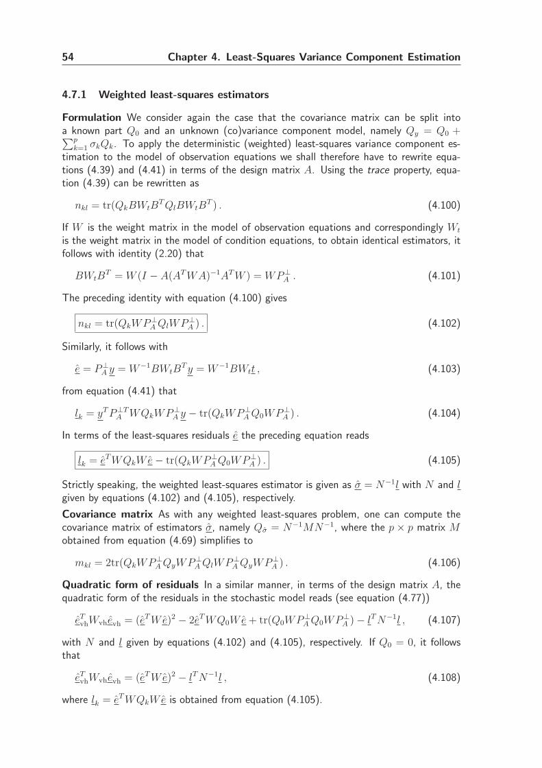
54 Chapter 4. Least-Squares Variance Component Estimation
4.7.1 Weighted least-squares estimators
Formulation We consider again the case that the covariance matrix can be split intoa known part Q0 and an unknown (co)variance component model, namely Qy = Q0 +∑p
k=1 σkQk. To apply the deterministic (weighted) least-squares variance component es-timation to the model of observation equations we shall therefore have to rewrite equa-tions (4.39) and (4.41) in terms of the design matrix A. Using the trace property, equa-tion (4.39) can be rewritten as
nkl = tr(QkBWtBT QlBWtB
T ) . (4.100)
If W is the weight matrix in the model of observation equations and correspondingly Wt
is the weight matrix in the model of condition equations, to obtain identical estimators, itfollows with identity (2.20) that
BWtBT = W (I − A(AT WA)−1AT W ) = WP⊥
A . (4.101)
The preceding identity with equation (4.100) gives
nkl = tr(QkWP⊥A QlWP⊥
A ) . (4.102)
Similarly, it follows with
e = P⊥A y = W−1BWtB
T y = W−1BWtt , (4.103)
from equation (4.41) that
lk = yT P⊥TA WQkWP⊥
A y − tr(QkWP⊥A Q0WP⊥
A ) . (4.104)
In terms of the least-squares residuals e the preceding equation reads
lk = eT WQkWe− tr(QkWP⊥A Q0WP⊥
A ) . (4.105)
Strictly speaking, the weighted least-squares estimator is given as σ = N−1l with N and lgiven by equations (4.102) and (4.105), respectively.
Covariance matrix As with any weighted least-squares problem, one can compute thecovariance matrix of estimators σ, namely Qσ = N−1MN−1, where the p × p matrix Mobtained from equation (4.69) simplifies to
mkl = 2tr(QkWP⊥A QyWP⊥
A QlWP⊥A QyWP⊥
A ) . (4.106)
Quadratic form of residuals In a similar manner, in terms of the design matrix A, thequadratic form of the residuals in the stochastic model reads (see equation (4.77))
eTvhWvhevh = (eT We)2 − 2eT WQ0We + tr(Q0WP⊥
A Q0WP⊥A )− lT N−1l , (4.107)
with N and l given by equations (4.102) and (4.105), respectively. If Q0 = 0, it followsthat
eTvhWvhevh = (eT We)2 − lT N−1l , (4.108)
where lk = eT WQkWe is obtained from equation (4.105).
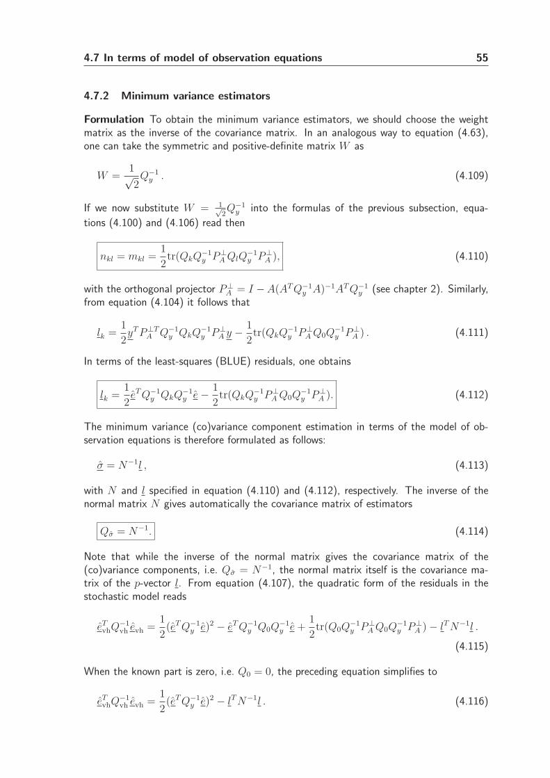
4.7 In terms of model of observation equations 55
4.7.2 Minimum variance estimators
Formulation To obtain the minimum variance estimators, we should choose the weightmatrix as the inverse of the covariance matrix. In an analogous way to equation (4.63),one can take the symmetric and positive-definite matrix W as
W =1√2Q−1
y . (4.109)
If we now substitute W = 1√2Q−1
y into the formulas of the previous subsection, equa-
tions (4.100) and (4.106) read then
nkl = mkl =1
2tr(QkQ
−1y P⊥
A QlQ−1y P⊥
A ), (4.110)
with the orthogonal projector P⊥A = I −A(AT Q−1
y A)−1AT Q−1y (see chapter 2). Similarly,
from equation (4.104) it follows that
lk =1
2yT P⊥T
A Q−1y QkQ
−1y P⊥
A y − 1
2tr(QkQ
−1y P⊥
A Q0Q−1y P⊥
A ) . (4.111)
In terms of the least-squares (BLUE) residuals, one obtains
lk =1
2eT Q−1
y QkQ−1y e− 1
2tr(QkQ
−1y P⊥
A Q0Q−1y P⊥
A ). (4.112)
The minimum variance (co)variance component estimation in terms of the model of ob-servation equations is therefore formulated as follows:
σ = N−1l , (4.113)
with N and l specified in equation (4.110) and (4.112), respectively. The inverse of thenormal matrix N gives automatically the covariance matrix of estimators
Qσ = N−1. (4.114)
Note that while the inverse of the normal matrix gives the covariance matrix of the(co)variance components, i.e. Qσ = N−1, the normal matrix itself is the covariance ma-trix of the p-vector l. From equation (4.107), the quadratic form of the residuals in thestochastic model reads
eTvhQ
−1vh evh =
1
2(eT Q−1
y e)2 − eT Q−1y Q0Q
−1y e +
1
2tr(Q0Q
−1y P⊥
A Q0Q−1y P⊥
A )− lT N−1l .
(4.115)
When the known part is zero, i.e. Q0 = 0, the preceding equation simplifies to
eTvhQ
−1vh evh =
1
2(eT Q−1
y e)2 − lT N−1l . (4.116)
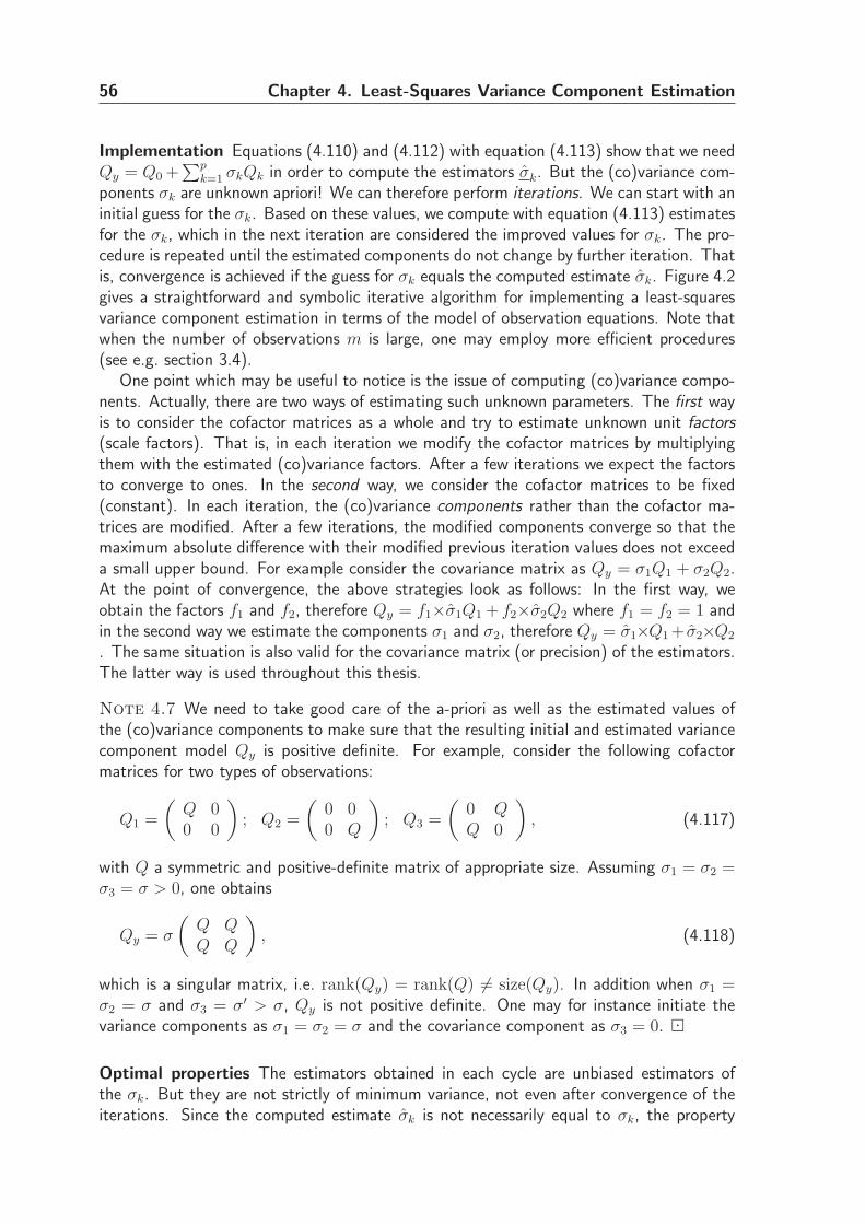
56 Chapter 4. Least-Squares Variance Component Estimation
Implementation Equations (4.110) and (4.112) with equation (4.113) show that we needQy = Q0 +
∑pk=1 σkQk in order to compute the estimators σk. But the (co)variance com-
ponents σk are unknown apriori! We can therefore perform iterations. We can start with aninitial guess for the σk. Based on these values, we compute with equation (4.113) estimatesfor the σk, which in the next iteration are considered the improved values for σk. The pro-cedure is repeated until the estimated components do not change by further iteration. Thatis, convergence is achieved if the guess for σk equals the computed estimate σk. Figure 4.2gives a straightforward and symbolic iterative algorithm for implementing a least-squaresvariance component estimation in terms of the model of observation equations. Note thatwhen the number of observations m is large, one may employ more efficient procedures(see e.g. section 3.4).
One point which may be useful to notice is the issue of computing (co)variance compo-nents. Actually, there are two ways of estimating such unknown parameters. The first wayis to consider the cofactor matrices as a whole and try to estimate unknown unit factors(scale factors). That is, in each iteration we modify the cofactor matrices by multiplyingthem with the estimated (co)variance factors. After a few iterations we expect the factorsto converge to ones. In the second way, we consider the cofactor matrices to be fixed(constant). In each iteration, the (co)variance components rather than the cofactor ma-trices are modified. After a few iterations, the modified components converge so that themaximum absolute difference with their modified previous iteration values does not exceeda small upper bound. For example consider the covariance matrix as Qy = σ1Q1 + σ2Q2.At the point of convergence, the above strategies look as follows: In the first way, weobtain the factors f1 and f2, therefore Qy = f1×σ1Q1 + f2×σ2Q2 where f1 = f2 = 1 andin the second way we estimate the components σ1 and σ2, therefore Qy = σ1×Q1 + σ2×Q2
. The same situation is also valid for the covariance matrix (or precision) of the estimators.The latter way is used throughout this thesis.
Note 4.7 We need to take good care of the a-priori as well as the estimated values ofthe (co)variance components to make sure that the resulting initial and estimated variancecomponent model Qy is positive definite. For example, consider the following cofactormatrices for two types of observations:
Q1 =
(Q 00 0
)
; Q2 =
(0 00 Q
)
; Q3 =
(0 QQ 0
)
, (4.117)
with Q a symmetric and positive-definite matrix of appropriate size. Assuming σ1 = σ2 =σ3 = σ > 0, one obtains
Qy = σ
(Q QQ Q
)
, (4.118)
which is a singular matrix, i.e. rank(Qy) = rank(Q) 6= size(Qy). In addition when σ1 =σ2 = σ and σ3 = σ′ > σ, Qy is not positive definite. One may for instance initiate thevariance components as σ1 = σ2 = σ and the covariance component as σ3 = 0. ⊡
Optimal properties The estimators obtained in each cycle are unbiased estimators ofthe σk. But they are not strictly of minimum variance, not even after convergence of theiterations. Since the computed estimate σk is not necessarily equal to σk, the property
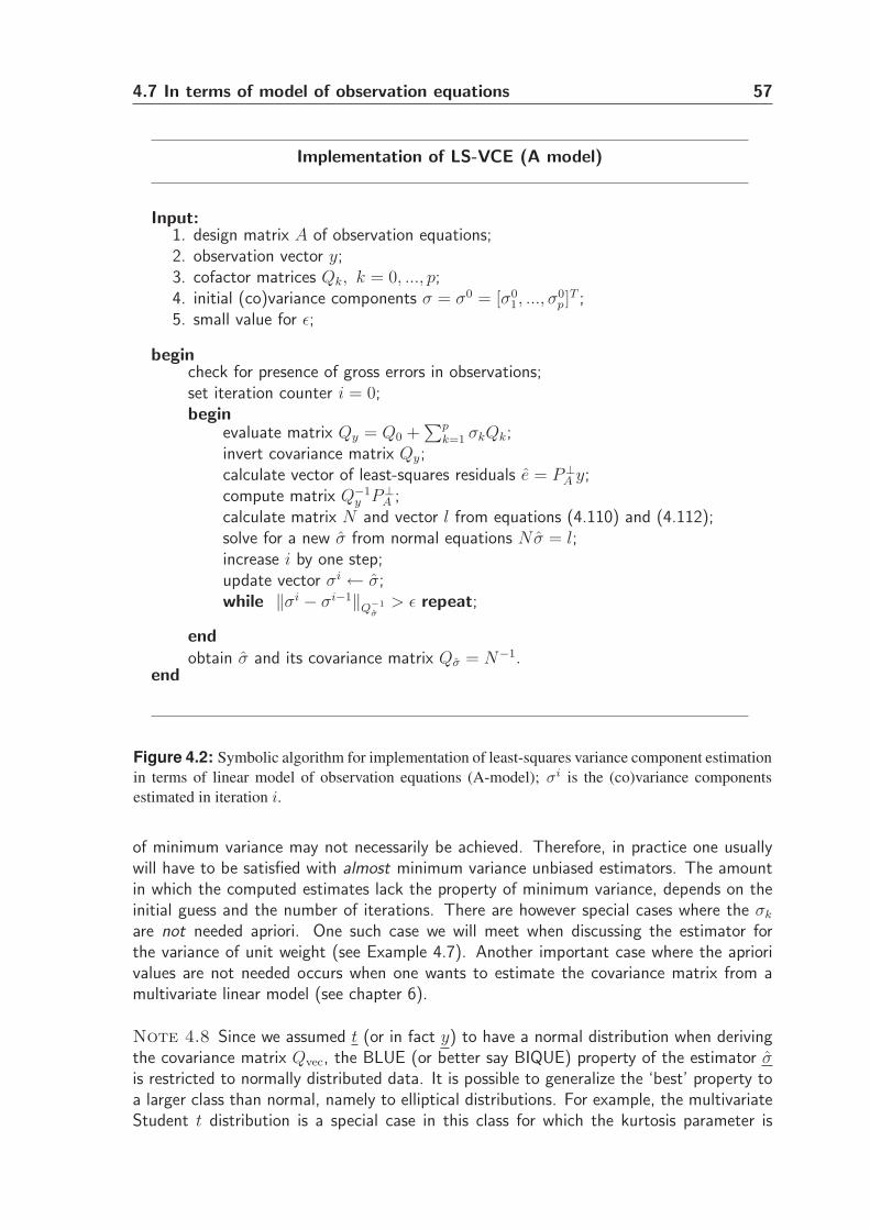
4.7 In terms of model of observation equations 57
Implementation of LS-VCE (A model)
Input:1. design matrix A of observation equations;2. observation vector y;3. cofactor matrices Qk, k = 0, ..., p;4. initial (co)variance components σ = σ0 = [σ0
1, ..., σ0p]
T ;5. small value for ǫ;
begincheck for presence of gross errors in observations;set iteration counter i = 0;begin
evaluate matrix Qy = Q0 +∑p
k=1 σkQk;invert covariance matrix Qy;calculate vector of least-squares residuals e = P⊥
A y;compute matrix Q−1
y P⊥A ;
calculate matrix N and vector l from equations (4.110) and (4.112);solve for a new σ from normal equations Nσ = l;increase i by one step;update vector σi ← σ;while ‖σi − σi−1‖Q−1
σ> ǫ repeat;
end
obtain σ and its covariance matrix Qσ = N−1.end
Figure 4.2: Symbolic algorithm for implementation of least-squares variance component estimation
in terms of linear model of observation equations (A-model); σi is the (co)variance components
estimated in iteration i.
of minimum variance may not necessarily be achieved. Therefore, in practice one usuallywill have to be satisfied with almost minimum variance unbiased estimators. The amountin which the computed estimates lack the property of minimum variance, depends on theinitial guess and the number of iterations. There are however special cases where the σk
are not needed apriori. One such case we will meet when discussing the estimator forthe variance of unit weight (see Example 4.7). Another important case where the apriorivalues are not needed occurs when one wants to estimate the covariance matrix from amultivariate linear model (see chapter 6).
Note 4.8 Since we assumed t (or in fact y) to have a normal distribution when derivingthe covariance matrix Qvec, the BLUE (or better say BIQUE) property of the estimator σis restricted to normally distributed data. It is possible to generalize the ‘best’ property toa larger class than normal, namely to elliptical distributions. For example, the multivariateStudent t distribution is a special case in this class for which the kurtosis parameter is
58 Chapter 4. Least-Squares Variance Component Estimation
not zero, κ = 2b−4
. The minimum variance estimators can thus be obtained for theclass of elliptically contoured distributed data (see Teunissen and Amiri-Simkooei, 2006).Therefore, if κ 6= 0, then Nσ = l with equations (4.110) and (4.112) does not strictlyprovide minimum variance estimators but only asymptotically ; i.e. when the redundancyin the functional model is large enough. The unbiasedness property of course still holds ingeneral. ⊡
Example 4.7 Let us as a simple application of the least-squares variance component estimationLS-VCE, assume that there is only one variance component in the stochastic model, namelyQy = σ2Q. If our original observables y are normally distributed, it follows with equations (4.110)and (4.112) from equation (4.113) that
σ2 =l
n=
12 eT Q−1
y QQ−1y e
12tr(QQ−1
y P⊥A QQ−1
y P⊥A )
, (4.119)
with the expectation and the variance of
E{σ2} = σ2 (unbiased) ; D{σ2} =2
tr(QQ−1y P⊥
A QQ−1y P⊥
A )≡ min (best) , (4.120)
respectively. With Qy = σ2Q, P⊥A P⊥
A = P⊥A , and tr(P⊥
A ) = rank(P⊥A ) = m − n = b, the
preceding equations simplify to
σ2 =eT Q−1e
m− n; E{σ2} = σ2 and D{σ2} =
2σ4
m− n. (4.121)
These are the well-known results for the estimator of the variance of unit weight. This estimatorcan thus be obtained from the least-squares residuals without any iteration. The least-squaresapproach implies that the above estimator is optimal in the sense that it is unbiased and hasminimum variance. With the least-squares approach we now also have a unified framework inwhich the well-known estimator of the variance of unit weight finds its logical place. That is, wenow do not have to introduce the estimator of the variance of unit weight in an ad hoc way! Inaddition, the quadratic form of residuals, i.e. equation (4.116) for our model, simplifies to
eTvhQ
−1vh evh =
b− 1
2b(eT Q−1
y e)2, (4.122)
with b = m−n the redundancy of the functional model. �
4.7.3 Nonlinear covariance function
Let us now consider a nonlinear (co)variance component model, namely Qy = Q(σ). Toovercome the nonlinearity, one can expand the stochastic model into a Taylor series. Forthis purpose we need to know the initial values for the unknown vector σ, namely σ0. Thelinear term of the Taylor series expansion reads
Qy = Q(σ0)−p∑
k=1
∂Q(σ)
∂σk
σk
∣∣∣∣σ0
+
p∑
k=1
∂Q(σ)
∂σk
∣∣∣∣σ0
σk . (4.123)
The above equation is in the form of the general (co)variance component model Qy =Q0 +
∑pk=1 σkQk with
Q0 = Q(σ0)−p∑
k=1
∂Q(σ)
∂σk
σk
∣∣∣∣σ0
; Qk =∂Q(σ)
∂σk
∣∣∣∣σ0
. (4.124)
4.7 In terms of model of observation equations 59
Implementation of non linear LS-VCE (A model)
Input:1. design matrix A of observation equations;2. observation vector y;3. function Q(σ) and its partial derivatives ∂σk
Q(σ), k = 1, ..., p ;4. initial (co)variance components σ = σ0 = [σ0
1, ..., σ0p]
T ;5. small value for ǫ;
begincheck for presence of gross errors in observations;set iteration counter i = 0;begin
obtain (modify) matrices Qik, k = 0, 1, ..., p, from equation (4.124);
evaluate matrix Qy = Q0 +∑p
k=1 σkQk;invert covariance matrix Qy;calculate vector of least-squares residuals e = P⊥
A y;compute matrix Q−1
y P⊥A ;
calculate matrix N and vector l from equations (4.110) and (4.112);solve for a new σ from normal equations Nσ = l;increase i by one step;update vector σi ← σ;while ‖σi − σi−1‖Q−1
σ> ǫ repeat;
end
obtain σ and its covariance matrix Qσ = N−1.end
Figure 4.3: Symbolic algorithm for implementation of nonlinear least-squares variance component
estimation in terms of linear model of observation equations.
We can now apply the least-squares method of the previous subsection to (co)variancecomponents. What we will estimate is the least-squares estimator for σ . The estimated σcan now be considered as a new update for σ0 and the same procedure can be repeated.We can iterate until the estimated (co)variance components do not change by furtheriterations. The Gauss-Newton iteration has a linear rate of convergence. This convergencerate is dictated by the normal curvature of the nonlinear manifold Avh(σ). For moreinformation we refer to Teunissen (1990).
Note 4.9 In the nonlinear LS-VCE, the cofactor matrices Qk, k = 1, ..., p are not fixed.They are modified from one iteration to the next. It is important to perceive that we havein fact two sorts of iterations for this model; one to come up with the nonlinearity andone due to the covariance matrix Qy which is unknown apriori. Because of the Taylorseries expansion, the initial values σ0 should be close enough to their final values. Roughapproximate values can lead to the divergence of the computed (co)variance components.The implementation algorithm is given in figure 4.3. ⊡
60 Chapter 4. Least-Squares Variance Component Estimation
4.8 Remarks on stochastic model
4.8.1 Negative variance components
Since the LS-VCE method is based on the ’unrestricted’ or ’unconstrained’ least-squaresprinciple, occurrence of negative variance components is not impossible. Estimated nega-tive variance components may result in a non-positive definite covariance matrix Qy, whichcan not be physically interpreted. Occurrence of negative variances makes sense whenwe compare the estimators with their precision (see equation (4.114)); they may not beprecise enough because of insufficient redundancy in the functional model. Though non-interpretable, a significantly negative variance component can be an important indicationof defects in our variance component model. We can enumerate at least
• an improperly designed (co)variance component model;The problem occurs when the (co)variance component model is not correct for thedata at hand. In this case one has to look for an appropriate stochastic model.In chapter 5 we introduce and employ hypotheses testing (e.g. w-test statistic) inconjunction with the least-squares variance component estimation. The methodprovides a powerful tool to look for a realistic stochastic model. The problem of animproperly designed stochastic model is thus not subject of discussion in this section.
• a low redundancy of our functional model;Low redundancy b of the functional model (and thereby df of stochastic model) cangive rise to some negative variance components. This also makes sense because theprecision of all parameters of interest directly depends on the number of observationsinvolved in the model. The more observations we have, the more precision for our(co)variance components we will obtain, and the less chance for estimators beinginadmissible (e.g. negative) we have.
Note 4.10 If the redundancy is too low, at times, the variance component modelbecomes singular. That is, we do not have enough observations for unique determi-nation of the unknowns in the stochastic model with that special structure. Theremight be different ways to handle the problem. One can for instance add more obser-vations to handle the problem (see next subsection). The other way, if allowed, is tomodify the stochastic model. The observations might be sufficient for estimating theparameters of a modified stochastic model. Low redundancy may also be interpretedas a weak functional model. Given the stochastic model, a weak functional modelmay lead to a high correlation between (co)variance components. Such estimatorsare usually of poor precision and occurrence of negative variances is more probable(see section 4.8.3). ⊡
• a badly chosen set of apriori (co)variance components (initial weight matrix W ).To avoid the non-negativity, one may for instance think of a proper set of a priorivalues for (co)variance components (a realistic weight matrix). That is, we try tochoose the initial components somewhat close to their actual values. The applicationof the so-called almost unbiased estimator must be useful. Since this estimator, aslong as the cofactor matrix Qk is semi-positive-definite, always results in a non-negative variance component, we can apply this method in the first iteration and
4.8 Remarks on stochastic model 61
then apply the least squares method. The almost unbiased estimator for the variancecomponent is given by Forstner (1979) (see also section 3.4).
Example 4.8 Consider one unknown quantity that is measured with two different instrumentstwice, i.e., y1, y2 and s1, s2. In the following, the design matrix, vector of observations, and twocofactor matrices are given as
A =
1111
, y =
y1
y2
s1
s2
, Q1 =
[I2 00 0
]
, Q2 =
[0 00 I2
]
. (4.125)
Assuming σ01 = 1 and σ0
2 = 1, i.e. W = I4 in equations (4.102) and (4.104), after a few simplemathematical operations, the estimated variance components read
σ1 = 16{3(y2
1 + y22) + 2(s1s2 − 2y1y2)− (s1 + s2)(y1 + y2)} ;
σ2 = 16{3(s2
1 + s22) + 2(y1y2 − 2s1s2)− (s1 + s2)(y1 + y2)} ,
(4.126)
which are not guaranteed to be positive all the time. Assume for instance observation valuesy1 = 10.0016 m, y2 = 10.0009 m, s1 = 9.9991 m, and s2 = 10.0036 m, which lead to a negativevariance component
[σ1
σ2
]
=
[−1.48
8.40
]
mm2 . (4.127)
Note that this is an example which leads to a negative variance component. One can find lotsof examples (different y in the above) with the resulting variances both being positive. Also ifone increases the number of observations, e.g. y3, s3, . . ., one will rarely encounter the negativevariance problem.
To see the role of the a-priori (co)variance components let us refer to the preceding results.For instance, if we choose the a-priori variance components as σ0
1 = 1 and σ02 = 10, the following
variance components can be estimated for the aforementioned sample (first iteration):
[σ1
σ2
]
=
[0.1985.463
]
mm2. (4.128)
After a few iterations, the converged solution is given as
[σ1
σ2
]
=
[0.2355.184
]
mm2, (4.129)
which are both positive. Note that the above structure for our model is known as a disjunctivegroup model with one variance component for each group. These components are expected tobe positive as the cofactor matrices Q1 and Q2 are both positive semi-definite. �
Non-negativity The (co)variance components are usually estimated in the absence of non-negative variance constraints. But in order to ensure non negative variance components,one may also incorporate non-negativity constraints σ ≥ 0 in equation (4.36). This leadsto a non-negative least squares problem. The standard form of the model of observationequations with non-negativity constraints is as follows: E{y} = Ax, x ≥ 0, D{y} = Qy
(cf. equation (2.4)). There are standard procedures for solving this problem (see e.g.Lawson and Hanson, 1974; Haskell and Hanson, 1981). One simple method to restore
62 Chapter 4. Least-Squares Variance Component Estimation
the non-negativeness is to reparameterize the variance components as follows (Teunissen,1988):
σi = eai , i = 1, · · · , p′ , (4.130)
where p′ is the number of variance components. If one solves for ai, namely ai, theestimated variance components then read
σi = eai , i = 1, · · · , p′ , (4.131)
which are forcefully and restrictively positive. The above reparameterization will lead usto a nonlinear (co)variance component model which was explained in section 4.7.3. Notethat estimation of the variance components, subject to non-negativity constraints, conflictswith unbiasedness property. But such estimators are definitely of lower minimum variancethan those obtained in the absence of the non-negativity constraints because we are usingthe additional information in a logical way.
4.8.2 Singular stochastic model
As previously mentioned, the (co)variance component model has a unique solution if andonly if the matrices BT Q1B, ..., BT QpB are linearly independent. If the cofactor matricesQ1, ..., Qp are linearly dependent, so are matrices BT Q1B, ..., BT QpB (i.e. rank deficientnormal matrix N). But if the cofactor matrices Q1, ..., Qp are linearly independent, thereis no guarantee for the stochastic model to have a unique solution. Therefore, linearindependence of the cofactor matrices Q1, ..., Qp is a necessary condition to have a fullrank normal matrix in the stochastic model. This is not however the sufficient condition,meaning that matrices BT Q1B, ..., BT QpB can be linearly dependent whereas Q1, ..., Qp
are linearly independent. To see this, we will consider two examples.
Example 4.9 Assume that we have observed an unknown quantity m times, i.e. a repeatedobservation. In this case we have the following model of observation equation:
E{y} = u x; D{y} = σ1I + σ2uuT , (4.132)
where u is the m×1 summation vector containing only ones. It is clear that the cofactor matricesQ1 = I and Q2 = uuT are linearly independent. One can however show that the unknowncovariance component σ2 is not estimable. Given the m× 1 design matrix A = u, it follows thatthe m×(m−1) matrix B in the model of condition equations reads B = [um−1 −Im−1]
T . ThenBT Q1B = um−1u
Tm−1+Im−1 and BT Q2B = 0. They are not linearly independent and therefore
σ2 remains inestimable. Note that increasing m can not overcome the singularity. Statisticallythis makes sense since strictly speaking a mutually constant covariance between observations,namely Q2 = uuT , can be interpreted as a systematic effect (constant bias) in the data. Such abias can not be estimated from the functional model of an unknown quantity because A = [u u]is also not of full rank (in fact the estimator x is biased by the systematic effect). Therefore, ifwe now try to estimate such a bias in the stochastic model, this also does not help. �
Let us now consider another simple example that the (co)variance components are notsimultaneously estimable.
4.8 Remarks on stochastic model 63
Example 4.10 Consider that we are measuring the same set of unknown quantities (e.g. dis-tances) with two different instruments which are in general of different precision. If we measurem different unknowns using these two instruments, then the number of unknowns is n = m,and the total number of observations would be 2m. The functional model which relates theobservations to the unknown parameters reads
E{y} = Ax, with y =
[y
1y
2
]
; A =
[II
]
. (4.133)
The redundancy of the functional model is b = 2m −m = m. In this example we have 2 typesof observations for which one needs to estimate a variance component (σ1 and σ2), and also acovariance component between y
1and y
2(σ3). The cofactor matrices may have the following
forms:
Q1 =
[Q 00 0
]
; Q2 =
[0 00 Q
]
; Q3 =
[0 QQ 0
]
, (4.134)
where Q is an arbitrary m×m symmetric and positive-definite matrix. The cofactor matrices Q1,Q2, and Q3 are linearly independent, but σ1, σ2, and σ3 are not simultaneously estimable. Toshow this, we need to obtain the matrix B of the model of condition equations. It is not difficultto see that B = [I − I]T . After a few simple mathematical operations one gets, BT Q1B = Q,BT Q2B = Q, and BT Q3B = −2Q. This means that the design matrix of the stochasticmodel, namely Avh, is not of full rank. In fact the 3 × 3 normal matrix N suffers from a rankdeficiency of two. Therefore, two out of three (co)variance components are not estimable; onlyone (co)variance component is estimable and not three. To handle the singularity of the above,at least, two ways are recommended.
1. assuming σ3 = 0 and the relative scale between Q1 and Q2 is known (e.g., they areequal σ1 = σ2), one can try to estimate a common variance component, namely Qy =σ1(Q1 + Q2);
2. assuming σ1 and σ2 are known, we can try to estimate the only covariance component σ3.If this is the case, one obtains Qy = Q0 + σ3Q3.
Generalization A third way can be to modify the functional and stochastic model by extendingthe observations plan. Let us consider 3 observation types instead of two kinds of observations,namely y1, y2 and y3. In this case, the VCE model consists of 3 cofactor matrices incorporatedwith 3 variance components, namely
A =
III
; Q1 =
Q 0 00 0 00 0 0
, Q2 =
0 0 00 Q 00 0 0
, Q3 =
0 0 00 0 00 0 Q
. (4.135)
The matrix B of the condition equations reads
B =
I I−I 0
0 −I
, (4.136)
which leads to the matrices
BT Q1B =
[Q QQ Q
]
; BT Q2B =
[Q 00 0
]
; BT Q3B =
[0 00 Q
]
. (4.137)
64 Chapter 4. Least-Squares Variance Component Estimation
The above listed cofactor matrices are linearly independent and therefore the variance compo-nents σ1, σ2 and σ3 are simultaneously estimable. One can simply show that if a covariancecomponent σ4 is in addition included between any two observation types, the stochastic modelbecomes singular. This shows that only three components out of six (co)variance componentsare estimable. To summarize, the above results can be generalized as follows: with r observationtypes and the above structure for the functional and stochastic model, we have r(r+1)
2 unknown
(co)variance components in total (r variance and r(r−1)2 covariance components). In this case
at maximum only r(r−1)2 out of r(r+1)
2 (co)variance components are estimable and the other rcomponents remain to be inestimable. �
Note 4.11 The aforementioned singular examples have nothing to do with the least-squares variance component estimation. This is in fact an intrinsic behavior (property)of the problem itself and is independent of the estimation principle which one applies tothe (co)variance component model. To handle the problem of the rank-deficient systemof normal equations Nσ = l some remedies were proposed. To handle the singularity onecan also either apply the theory of generalized inverses (see e.g. Rao and Mitra (1971)),or apply the theory of S-transformations (see Baarda, 1973; Teunissen, 1985). ⊡
4.8.3 Ill-posedness of stochastic model
As mentioned, the normal matrix N of the VCE formulas will become singular if and onlyif the matrices BT Q1B, ..., BT QpB are linearly dependent. If the matrix N is strictly rankdeficient then the cofactor matrices are linearly dependent. But practically, N , sometimes,is nearly rank-deficient (ill-conditioned) rather than strictly rank deficient. This means,theoretically, that N is of full rank but practically the solution is severely sensitive toround-off and random errors; so the solution is not stable. In this case, usually, one ormore functions of the estimators may have very poor precision. To handle the problem, wesuggest to compute the condition number of N .
For the positive-definite matrix N , the condition number is defined as the ratio c =λmax/λmin, with λmax and λmin the maximum and minimum eigenvalues of the matrix,respectively. For such a matrix, the solution σ = N−1l and the error δσ = N−1δl alwayssatisfy the inequality (Strang, 1988)
‖δσ‖ ≤ c‖σ‖‖l‖ ‖δl‖, or
‖δσ‖‖σ‖ ≤ c
‖δl‖‖l‖ , (4.138)
where ‖.‖ denotes the norm of a vector. The above equation, in a relative sense, shows thatany error ‖δl‖ in the observations, both rounding and random errors, is amplified into thesolution (at maximum) by the condition number. Ideally, for a well-conditioned matrix, thecondition number is one, e.g., an identity matrix. This implies that the condition number cis not directly affected by the size of the matrix; so it is a better measure of ill-conditioningthan the determinant. If c is large, the solution is ill-conditioned and thus the cofactormatrices BT Q1B, ..., BT QpB are nearly linearly dependent. It is important to perceive,at times, that the cofactor matrices Q1, ..., Qp are strictly independent but the problem isill-posed. This can be the case when combining non-precise observations with precise ones(e.g. when combining GPS code and phase observations; see chapter 7).
Since the condition number depends on the type of the formulation of the problem, and,in addition, it is an overall measure, meaning that it does not employ all information in an
4.8 Remarks on stochastic model 65
optimal way, it is suggested to evaluate the degree of dependency of the columns of thedesign matrix Avh in equation (4.15). For this purpose we consider the following partitionof the design matrix of the stochastic model:
(AJ...aj); j = 2, 3, . . . , p, J = {1, 2, . . . , j − 1} , (4.139)
where AJ contains the first j − 1 columns of the VCE design matrix Avh and aj is the jth
column of the matrix Avh and its dependency from AJ is to be evaluated. Let θj be theangle between aj and R(AJ). Then, the degree of dependence θj between aj and R(AJ)can be obtained from the following equation:
sin2θj
=aT
j Q−1vh aj
aTj Q−1
vh aj
, j = 2, . . . , p , (4.140)
where
aTj Q−1
vh aj = aTj Q−1
vh aj − aTj Q−1
vh AJ(ATJ Q−1
vh AJ)−1ATJ Q−1
vh aj . (4.141)
The above measure can be simply obtained by some elements of the normal matrix asfollows:
sin2θj
=njj −NjJN−1
JJ NJj
njj
; j = 2, . . . , p . (4.142)
The term NJJ = ATJ Q−1
vh AJ is the (j − 1)× (j − 1) normal matrix part corresponding toAJ , NJj = AT
J Q−1vh aj is a j−1 vector containing the first j−1 elements of the jth column
of N , and njj = aTj Q−1
vh aj is the jth diagonal element of N . The above equation can besimplified to the following:
cos2θj
=NjJN−1
JJ NJj
njj
, j = 2, . . . , p . (4.143)
When dealing with two unknown components, p = 2, the above equation is reduced to thefollowing simple formula:
cosθ =±n12√n11 n22
, (4.144)
which represents a correlation coefficient ρ. If θ = π/2, then aj is orthogonal to (fullyindependent of) R(AJ); i.e. ρ = 0. On the other hand, if θ = 0, then aj belongs to therange space of AJ (fully dependent); i.e. ρ = ±1. If θ is small, then aj nearly belongs toR(AJ) and therefore σj is poorly estimable.
Example 4.11 To see how the preceding measures work, in example 4.10 consider m = 2 andσ3 = 0. If we now assume that the cofactor matrices Q1 and Q2 have the form
Q1 =
[I2 00 0
]
; Q2 =
[0 00 Q
]
with Q =
[1 αα 1
]
, (4.145)
with −1 < α < 1, α 6= 0. Taking the above cofactor matrices into account and assuming theweight matrix as W = (Q1 + Q2)
−1 (i.e. in the first iteration σ01 = σ0
2 = 1) and after not soshort mathematical and matrix operations, the normal matrix of the stochastic model reads
N =1
(4− α2)2
[4 + α2 4− 3α2
4− 3α2 4− 3α2 + α4
]
; −1 < α < 1 , (4.146)
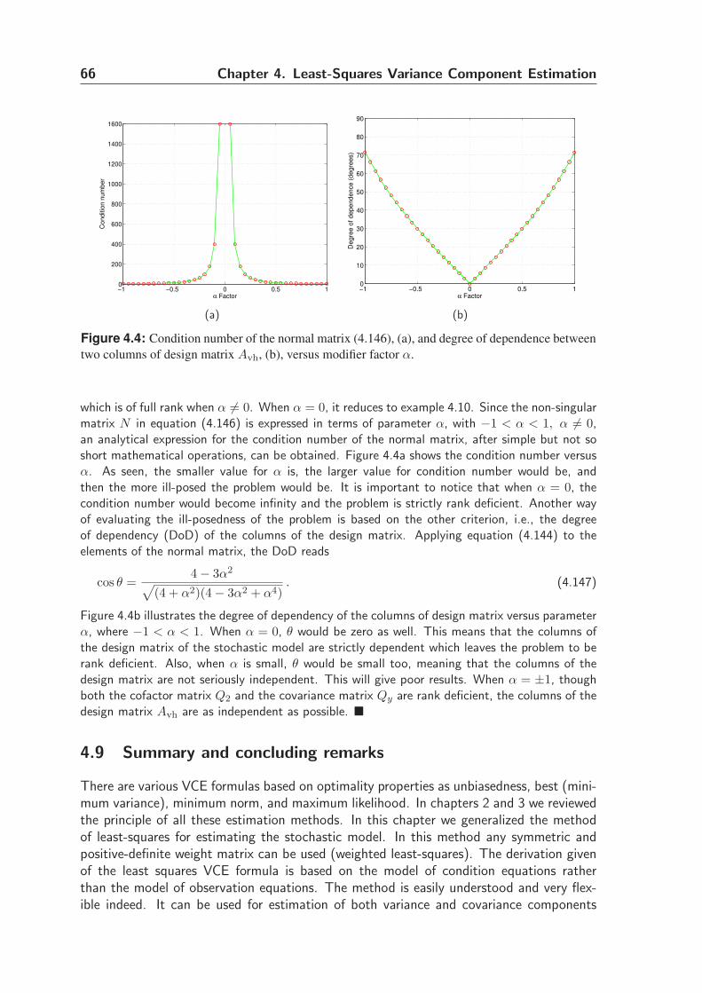
66 Chapter 4. Least-Squares Variance Component Estimation
−1 −0.5 0 0.5 10
200
400
600
800
1000
1200
1400
1600
α Factor
Conditio
n n
um
ber
(a)
−1 −0.5 0 0.5 10
10
20
30
40
50
60
70
80
90
α Factor
Degre
e o
f dependence (
degre
es)
(b)
Figure 4.4: Condition number of the normal matrix (4.146), (a), and degree of dependence between
two columns of design matrix Avh, (b), versus modifier factor α.
which is of full rank when α 6= 0. When α = 0, it reduces to example 4.10. Since the non-singularmatrix N in equation (4.146) is expressed in terms of parameter α, with −1 < α < 1, α 6= 0,an analytical expression for the condition number of the normal matrix, after simple but not soshort mathematical operations, can be obtained. Figure 4.4a shows the condition number versusα. As seen, the smaller value for α is, the larger value for condition number would be, andthen the more ill-posed the problem would be. It is important to notice that when α = 0, thecondition number would become infinity and the problem is strictly rank deficient. Another wayof evaluating the ill-posedness of the problem is based on the other criterion, i.e., the degreeof dependency (DoD) of the columns of the design matrix. Applying equation (4.144) to theelements of the normal matrix, the DoD reads
cos θ =4− 3α2
√
(4 + α2)(4− 3α2 + α4). (4.147)
Figure 4.4b illustrates the degree of dependency of the columns of design matrix versus parameterα, where −1 < α < 1. When α = 0, θ would be zero as well. This means that the columns ofthe design matrix of the stochastic model are strictly dependent which leaves the problem to berank deficient. Also, when α is small, θ would be small too, meaning that the columns of thedesign matrix are not seriously independent. This will give poor results. When α = ±1, thoughboth the cofactor matrix Q2 and the covariance matrix Qy are rank deficient, the columns of thedesign matrix Avh are as independent as possible. �
4.9 Summary and concluding remarks
There are various VCE formulas based on optimality properties as unbiasedness, best (mini-mum variance), minimum norm, and maximum likelihood. In chapters 2 and 3 we reviewedthe principle of all these estimation methods. In this chapter we generalized the methodof least-squares for estimating the stochastic model. In this method any symmetric andpositive-definite weight matrix can be used (weighted least-squares). The derivation givenof the least squares VCE formula is based on the model of condition equations ratherthan the model of observation equations. The method is easily understood and very flex-ible indeed. It can be used for estimation of both variance and covariance components
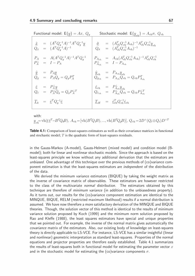
4.9 Summary and concluding remarks 67
Functional model: E{y} = Ax, Qy Stochastic model: E{yvh} = Avhσ, Qvh
x = (AT Q−1y A)−1AT Q−1
y y σ = (ATvhQ
−1vh Avh)
−1ATvhQ
−1vh y
vh
Qx = (AT Q−1y A)−1 Qσ = (AT
vhQ−1vh Avh)
−1
PA = A(AT Q−1y A)−1AT Q−1
y PAvh= Avh(A
TvhQ
−1vh Avh)
−1ATvhQ
−1vh
P⊥A = I − PA P⊥
Avh= I − PAvh
y = PAy yvh
= PAvhy
vh
Qy = PAQy = QyPTA Qyvh
= PAvhQvh = QvhP
TAvh
e = P⊥A y evh = P⊥
Avhy
vh
Qe = P⊥A Qy = QyP
⊥TA Qevh
= P⊥Avh
Qvh = QvhP⊥TAvh
T b = eT Q−1y e T df = eT
vhQ−1vh evh
with:y
vh=vh(t tT−BTQ0B), Avh =[vh(BTQ1B), ..., vh(BTQpB)], Qvh =2D+(Qt⊗Qt)D
+T
Table 4.1: Comparison of least-squares estimators as well as their covariance matrices in functional
and stochastic model; T is the quadratic form of least-squares residuals.
in the Gauss-Markov (A-model), Gauss-Helmert (mixed model) and condition model (B-model); both for linear and nonlinear stochastic models. Since the approach is based on theleast-squares principle we know without any additional derivation that the estimators areunbiased. One advantage of this technique over the previous methods of (co)variance com-ponent estimation is that the least-squares estimators are independent of the distributionof the data.
We derived the minimum variance estimators (BIQUE) by taking the weight matrix asthe inverse of covariance matrix of observables. These estimators are however restrictedto the class of the multivariate normal distribution. The estimators obtained by thistechnique are therefore of minimum variance (in addition to the unbiasedness property).As it turns out, our results for the (co)variance component estimation are identical to theMINQUE, BIQUE, RELM (restricted maximum likelihood) results if a normal distribution isassumed. We have now therefore a more satisfactory derivation of the MINQUE and BIQUEtheories. Though, the solution vector of this method is identical to the results of minimumvariance solution proposed by Koch (1999) and the minimum norm solution proposed byRao and Kleffe (1988), the least squares estimators have special and unique propertiesthat we pointed out. For example, the inverse of the normal matrix gives automatically thecovariance matrix of the estimators. Also, our existing body of knowledge on least-squarestheory is directly applicable to LS-VCE. For instance, LS-VCE has a similar insightful (linearand nonlinear) geometric interpretation as standard least-squares. Properties of the normalequations and projector properties are therefore easily established. Table 4.1 summarizesthe results of least-squares both in functional model for estimating the parameter vector xand in the stochastic model for estimating the (co)variance components σ.

68 Chapter 4. Least-Squares Variance Component Estimation
Since the method is based on the least-squares principle, measures of inconsistency, suchas the quadratic form of residuals and the w-test statistic can directly be given. We canalso apply testing hypotheses with the stochastic model. This, as an important feature ofLS-VCE, is the subject of discussion in the next chapter.
Detection and Validation in Stochastic Model 55.1 Introduction
In this chapter we generalize the idea of detection and validation introduced in chapter 2into the stochastic model. The goal is to find misspecifications in the stochastic model,or to improve an existing covariance matrix description by including more (or excluding)(co)variance components. This can be done by introducing the w-test, the v-test, and theoverall model test with the stochastic model. We show that employing the w-test and v-testin the stochastic model is in fact equivalent to the testing of (co)variance components.
We will point out the limitations of using the proposed formulations. Note that becausethe observables, here in the stochastic model, are in a quadratic form of the originalobservables y or t, i.e. vh(y yT ) or vh(t tT ), the distribution of the test statistics becomes(much) more complicated when compared to the functional model. For example, the overallmodel test has the most complicated form of the distribution. This chapter is thereforeconsidered as a first attempt for the detection and validation in the stochastic model.
5.2 The w-test statistic
5.2.1 Introduction
The goal of this section is to generalize the square-root of the 1-dimensional T-test statisticor the w-test statistic introduced in chapter 2 to the stochastic model. In the functionalmodel, the w-test statistic is given by equations (2.39) and (2.42). In a similar way to thefunctional model, it is also possible, for the stochastic model, to obtain the w-test statisticand to generalize the idea of datasnooping on the vector vh(t tT ).
The hypotheses that will be considered in this section are all hypotheses on the meanof the observable vector vh(t tT ) in the stochastic model. Such hypotheses are in factequivalent to those considered on the (co)variance components of covariance matrix Qt.From the explicit form of the observation equations of the VCE model, the following twohypotheses are put forward:
Ho : E{vh(t tT )} = Avhσ versus Ha : E{vh(t tT )} = Avhσ + cvh∇, ∇ 6= 0 , (5.1)
The design matrix Avh is supposed to be of full column rank, i.e. rank(Avh) = p.Furthermore, vector cvh is independent of the range space of the matrix Avh, i.e.rank(Avh : cvh) = p + 1. The scalar ∇ is unknown under Ha. Because both vh andE are linear operators, the above null and alternative hypotheses can be reformulated as
70 Chapter 5. Detection and Validation in Stochastic Model
follows:
Ho : E{t tT} = BT Q0B +
p∑
k=1
σkBT QkB, (5.2)
versus
Ha : E{t tT} = BT Q0B +
p∑
k=1
σkBT QkB + Ct∇, ∇ 6= 0 , (5.3)
where the b×b symmetric matrix Ct satisfies cvh = vh(Ct). The constant term BT Q0B hasbeen included to keep the generality of the formulation. When there is no misspecificationin the functional part of the model, namely when E{y} = Ax or E{t} = 0, it follows that
E{t tT} = Qt which yields
Ho : Qt = BT Q0B +
p∑
k=1
σkBT QkB , (5.4)
versus
Ha : Qt = BT Q0B +
p∑
k=1
σkBT QkB + Ct∇, ∇ 6= 0 . (5.5)
The above formulation can be used for finding misspecifications in the covariance matrixof the misclosure vector t, i.e. Qt. The preceding hypotheses, in fact, provides us witha powerful tool to judge whether or not additional (co)variance components are likelyto be included in the stochastic model. Note, however, that in most Geodesy and GPSapplications, one needs to evaluate the misspecification in the covariance matrix of theoriginal observables y, namely Qy, rather than Qt (see section 5.2.5). From now on, for the
sake of brevity, we will ignore the constant term Qt0 = BT Q0B in our derivations, but whenneeded, we will make a few comments on that. Also, the matrices BT Q1B, ..., BT QpBare simply denoted as Qt1 , ..., Qtp . In addition, the statement ∇ 6= 0 in the alternativehypothesis will be disregarded (simply note that ∇ is always non-zero).
Carrying through the similarity with the functional model, we will just try to obtainequation (2.42) for the stochastic model and to determine its distribution under Ho as-suming the original observables y or misclosures t to be normally distributed. The w-teststatistic for the stochastic model reads then (cf. equation (2.42))
w =〈P⊥
Avhvh(Ct), P
⊥Avh
vh(t tT )〉‖P⊥
Avhvh(Ct)‖Q−1
vh
= ‖evh‖Q−1vh
cos ϕ , (5.6)
where most of the terms are given in table 4.1. Note that ϕ is the angle between two vectorsP⊥
Avhvh(Ct) and P⊥
Avhvh(t tT ). In the next subsection, we will give a simple expression for
the preceding formula. The above test statistic has a similar geometrical interpretation tothat introduced in section 2.2.4 with the functional model.
5.2 The w-test statistic 71
5.2.2 Formulation in terms of B-model
To obtain a simple expression for the w-test, one needs to reach a simplified formula forthe norm and the inner product (in metric Q−1
vh ) in equation (5.6). For this purpose, let usconsider the following theorem:
Theorem 5.1 Let the b× b matrices Z1 and Z2 be symmetric. Then
⟨P⊥
Avhvh(Z1) , P⊥
Avhvh(Z2)
⟩=
1
2tr(Z1Q
−1t Z2Q
−1t )− g(1)T N−1g(2) , (5.7)
where 〈. , .〉 denotes the inner (scalar) product of two vectors in the metric Q−1vh and the
p-vector g(1) is given as
g(1)k =
1
2tr(Z1Q
−1t QtkQ
−1t ), k = 1, 2, ..., p , (5.8)
and so is g(2) with Z2. When Z2 = Z1, the inner product becomes the squared norm (L2
norm) of P⊥Avh
vh(Z1). Therefore
‖P⊥Avh
vh(Z1)‖2Q−1vh
=1
2tr(Z1Q
−1t Z1Q
−1t )− g(1)T N−1g(1) , (5.9)
where ‖.‖Q−1vh
denotes the norm of a vector in the metric Q−1vh . ⊠
Proof. The inner product of vectors P⊥Avh
vh(Z1) and P⊥Avh
vh(Z2), in the metric Q−1vh , is given
as⟨
P⊥Avh
vh(Z1) , P⊥Avh
vh(Z2)⟩
= vh(Z1)T P⊥T
AvhQ−1
vh P⊥Avh
vh(Z2) . (5.10)
Since P⊥TAvh
Q−1vh P⊥
Avh= Q−1
vh P⊥Avh
, the preceding equation reads
⟨
P⊥Avh
vh(Z1) , P⊥Avh
vh(Z2)⟩
= vh(Z1)T Q−1
vh P⊥Avh
vh(Z2) . (5.11)
If we now substitute the terms vh(.) = D+vec(.), Q−1vh = 1
2DT (Q−1t ⊗ Q−1
t )D, and P⊥Avh
=
I−AvhN−1AT
vhQ−1vh in the preceding equation, one can leave out, similar to previous derivations
of chapter 4, the duplication matrices D and simply prove the theorem. The second part of thetheorem is trivial. H
Because of the symmetry of the b× b matrices Ct and t tT , if we now substitute Z1 = Ct
and Z2 = t tT , it follows from equation (5.6) with theorem 5.1 that
w =wn
wd=
12tr(CtQ
−1t t tT Q−1
t )− gT N−1l[
12tr(CtQ
−1t CtQ
−1t )− gT N−1g
]1/2, (5.12)
with g and l respectively as
gk =1
2tr(CtQ
−1t QtkQ
−1t ); lk =
1
2tT Q−1
t QtkQ−1t t . (5.13)
72 Chapter 5. Detection and Validation in Stochastic Model
Note 5.1 (Summation convention) In the sequel, summation∑
, for the sake ofbrevity, is sometimes disregarded. This is based on the summation convention which statesthat whenever there arises an expression in which an index occurs twice on the same sideof any equation, or term within an equation, it is understood to represent a summation onthese repeated indices. A repeated index is called a summation index, while an unrepeatedindex is called a free index. For example, the trace of a matrix S can simply be denotedas tr(S) = sii while the matrix itself is symbolized as S = sij. ⊡
With the summation convention and substituting ll = 12tT Q−1
t QtlQ−1t t, the numerator of
the w-test statistic in equation (5.12) is rewritten as
wn = 12tT Q−1
t CtQ−1t t− 1
2gkn
−1kl tT Q−1
t QtlQ−1t t
= 12tT Q−1
t CtQ−1t t− 1
2tT Q−1
t [gkn−1kl Qtl ]Q
−1t t
= tT Q−1t
(12Ct − 1
2[gkn
−1kl Qtl ]
)Q−1
t t .
(5.14)
Substitution of the preceding equation into equation (5.12) yields
w = tT Mt =tT Q−1
t
(12Ct − 1
2[gkn
−1kl Qtl ]
)Q−1
t t[
12tr(CtQ
−1t CtQ
−1t )− gT N−1g
]1/2, (5.15)
with the symmetric matrix M as
M =Q−1
t
(12Ct − 1
2[gkn
−1kl Qtl ]
)Q−1
t[
12tr(CtQ
−1t CtQ
−1t )− gT N−1g
]1/2, (5.16)
Therefore, the w-test statistic of the stochastic model can be written as a quadratic form inthe vector t which is supposed to be normally distributed. This is an important result sincethe distribution of quadratic forms can be derived. This can be considered an importantissue if one wants to apply hypotheses testing and to compute the critical values of the test.Note that, if a constant term Qt0 = BT Q0B is also included in both null and alternativehypotheses, the numerator of equation (5.15) should be added up with the constant term−1
2tr(CtQ
−1t Qt0Q
−1t ).
Note 5.2 The symmetric matrix Ct should be linearly independent from the matricesQt1 , ..., Qtp . Otherwise, the w-test can not be defined since zero over zero is undefined.To see this, let us assume that Ct is a linear combination of Qt1 , ..., Qtp
Ct =
p∑
i=1
αiBT QiB =
p∑
i=1
αiQti = αiQti , (5.17)
with αi some non-zero real numbers. Substituting the preceding equation in equation (5.13)gives gk = 1
2tr(αiQtiQ
−1t QtkQ
−1t ) = αinik. Substituting Ct = αiQti and gk = αinik into
the numerator of equation (5.15), namely wn, gives
wn =1
2αit
T Q−1t
(Qti − [nikn
−1kl Qtl ]
)Q−1
t t, (5.18)
5.2 The w-test statistic 73
in which nikn−1kl , multiplication of the ith, i = 1, ..., p row of N with the lth, l = 1, ..., p
column of N−1, is the well-known Kronecker delta, i.e.
nikn−1kl = δil =
{1 if i = l ;0 if i 6= l .
(5.19)
Substituting nikn−1kl = δil in equation (5.18) yields
wn =1
2αit
T Q−1t (Qti −Qti) Q−1
t t = 0 . (5.20)
In an analogous way, one can show that the denominator of equation (5.15) simplifies to
wd =[αT Nα− αT Nα
]1/2= 0 , (5.21)
which proves the claim. In the next subsections, we show how to formulate matrix Ct. ⊡
Special case 5.1 (1) In some applications the covariance matrix is known under the null hy-pothesis, i.e. Ho : Qt = Qt0 versus Ho : Qt = Qt0 + Ct∇. Therefore, there is no unknownin the stochastic model to estimate. In this case, the normal matrix N is empty. The w-teststatistic can therefore be given from equation (5.15) when the constant term Qt0 is included inthe formulation
w =12
[tT Q−1
t CtQ−1t t− tr(CtQ
−1t )]
[12tr(CtQ
−1t CtQ
−1t )]1/2
, (5.22)
which has in fact a very simple form. The above w-test may be written as w = tT Mt−m0 with
M =12Q−1
t CtQ−1t
[12tr(CtQ
−1t CtQ
−1t )]1/2
; m0 =12tr(CtQ
−1t )
[12tr(CtQ
−1t CtQ
−1t )]1/2
. (5.23)
The constant m0 only changes the mean of the statistic tT Mt (just shifts it into the origin). �
Special case 5.2 (2) Another special case of the w-test occurs when only one variance compo-nent is involved in the stochastic model, p = 1. The null and alternative hypotheses are givenas
Ho : Qt = σ1Qt1 versus Ha : Qt = σ1Qt1 + Ct∇ , (5.24)
with σ1 = σ2 the variance of unit weight. Under the null hypothesis one obtains
Qy = σ2Q1 and Q−1t =
1
σ2(BT Q1B)−1 =
1
σ2Q−1
t1. (5.25)
The scalars l, g, and N read then (note that p = 1)
l = l1 = 12 tT Q−1
t Qt1Q−1t t = 1
2σ2 tT Q−1t t ;
g = g1 = 12tr(CtQ
−1t Qt1Q
−1t ) = 1
2σ2 tr(CtQ−1t ) ;
N = n11 = 12tr(Q−1
t Qt1Q−1t Qt1) = b
2σ4 .
(5.26)
Substituting g and N in equation (5.15) yields the w-test as
w = tT Mt =tT Q−1
t
[12Ct − tr(CtQ
−1t )
2b Qt
]
Q−1t t
[12tr(CtQ
−1t CtQ
−1t )− 1
2btr(CtQ−1t )tr(CtQ
−1t )]1/2
. (5.27)
In the sequel, we will refer to these two special cases several times. �
74 Chapter 5. Detection and Validation in Stochastic Model
5.2.3 Distribution of w-test statistic
In order to derive the distribution of the w-test statistic for the stochastic model, we needthe distribution of w = tT Mt given in the previous subsection. It is based on the followingtheorem, the distribution of quadratic forms in normal variables. We closely but not exactlyfollow Teunissen (1988).
Theorem 5.2 Let the b × 1 vector t be normally distributed with mean E{t} = 0 andpositive definite covariance matrix Qt. Let M be a symmetric matrix of order b. Thenthere exists a diagonal matrix Λr = diag(λ1, λ2, · · · , λr) such that
tT Mt = zT Λrz =r∑
i=1
λiz2i , (5.28)
where z has the standard normal distribution, i.e. z ∼ N(0, Ir). The number r is the rankof M or MQt. The diagonal elements of Λr are the r eigenvalues of MQt or QtM . ⊠
Proof. If we define the random vector x = Q−1/2t t, then clearly x has a standard normal distrib-
ution, i.e. x ∼ N(0, Ib). Substitution of t = Q1/2t x in tT Mt gives
tT Mt = xT Q1/2t MQ
1/2t x . (5.29)
Since the matrix Q1/2t MQ
1/2t is symmetric, it has real-valued eigenvalues (not necessarily positive)
and corresponding orthonormal eigenvectors. In case M is of full rank (b = r), if we collect the b-number of non-zero eigenvalues in the b×b diagonal matrix Λ and the corresponding orthonormaleigenvectors as columns in the b× b matrix U then
Q1/2t MQ
1/2t = UΛUT , (5.30)
with
UT U = UUT = Ib . (5.31)
If rank(Q1/2t MQ
1/2t ) = r < b, then r-number of eigenvalues are non-zero and (b− r)-number of
eigenvalues are zero. We may therefore partition equation (5.30) as
Q1/2t MQ
1/2t = [Ur Ub−r]
[Λr 00 0
] [UT
r
UTb−r
]
= UrΛrUTr , (5.32)
with
UTr Ur = Ir (5.33)
Substitution of equation (5.32) into equation (5.29) gives
tT Mt = xT UrΛrUTr x = zT Λrz , (5.34)
with
z = UTr x = UT
r Q−1/2t t . (5.35)
Since x is distributed as x ∼ N(0, Ib), and UTr Ur = Ir, it follows that z = UT
r x is distributed as
z ∼ N(0, Ir). Note that since |Q1/2t MQ
1/2t −λIb| = |MQt−λIb| = |QtM−λIb|, the eigenvalues
of Q1/2t MQ
1/2t , MQt and QtM are the same. H
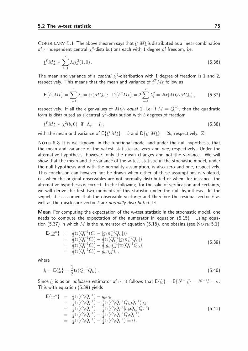
5.2 The w-test statistic 75
Corollary 5.1 The above theorem says that tT Mt is distributed as a linear combinationof r independent central χ2-distributions each with 1 degree of freedom, i.e.
tT Mt ∼r∑
i=1
λiχ2i (1, 0) . (5.36)
The mean and variance of a central χ2-distribution with 1 degree of freedom is 1 and 2,respectively. This means that the mean and variance of tT Mt follow as
E{tT Mt} =r∑
i=1
λi = tr(MQt); D{tT Mt} = 2r∑
i=1
λ2i = 2tr(MQtMQt) , (5.37)
respectively. If all the eigenvalues of MQt equal 1, i.e. if M = Q−1t , then the quadratic
form is distributed as a central χ2-distribution with b degrees of freedom
tT Mt ∼ χ2(b, 0) if Λr = Ib , (5.38)
with the mean and variance of E{tT Mt} = b and D{tT Mt} = 2b, respectively. ⊠
Note 5.3 It is well-known, in the functional model and under the null hypothesis, thatthe mean and variance of the w-test statistic are zero and one, respectively. Under thealternative hypothesis, however, only the mean changes and not the variance. We willshow that the mean and the variance of the w-test statistic in the stochastic model, underthe null hypothesis and with the normality assumption, is also zero and one, respectively.This conclusion can however not be drawn when either of these assumptions is violated,i.e. when the original observables are not normally distributed or when, for instance, thealternative hypothesis is correct. In the following, for the sake of verification and certainty,we will derive the first two moments of this statistic under the null hypothesis. In thesequel, it is assumed that the observable vector y and therefore the residual vector e aswell as the misclosure vector t are normally distributed. ⊡
Mean For computing the expectation of the w-test statistic in the stochastic model, oneneeds to compute the expectation of the numerator in equation (5.15). Using equa-tion (5.37) in which M is the numerator of equation (5.16), one obtains (see Note 5.1)
E{wn} = 12tr(Q−1
t (Ct − [gkn−1kl Qtl ]))
= 12tr(Q−1
t Ct)− 12tr(Q−1
t [gkn−1kl Qtl ])
= 12tr(Q−1
t Ct)− 12[gkn
−1kl ]tr(Q−1
t Qtl)= 1
2tr(Q−1
t Ct)− gkn−1kl ll ,
(5.39)
where
ll = E{ll} =1
2tr(Q−1
t Qtl) . (5.40)
Since σ is as an unbiased estimator of σ, it follows that E{σ} = E{N−1l} = N−1l = σ.This with equation (5.39) yields
E{wn} = 12tr(CtQ
−1t )− gkσk
= 12tr(CtQ
−1t )− 1
2tr(CtQ
−1t QtkQ
−1t )σk
= 12tr(CtQ
−1t )− 1
2tr(CtQ
−1t [σkQtk ]Q
−1t )
= 12tr(CtQ
−1t )− 1
2tr(CtQ
−1t QtQ
−1t )
= 12tr(CtQ
−1t )− 1
2tr(CtQ
−1t ) = 0 .
(5.41)
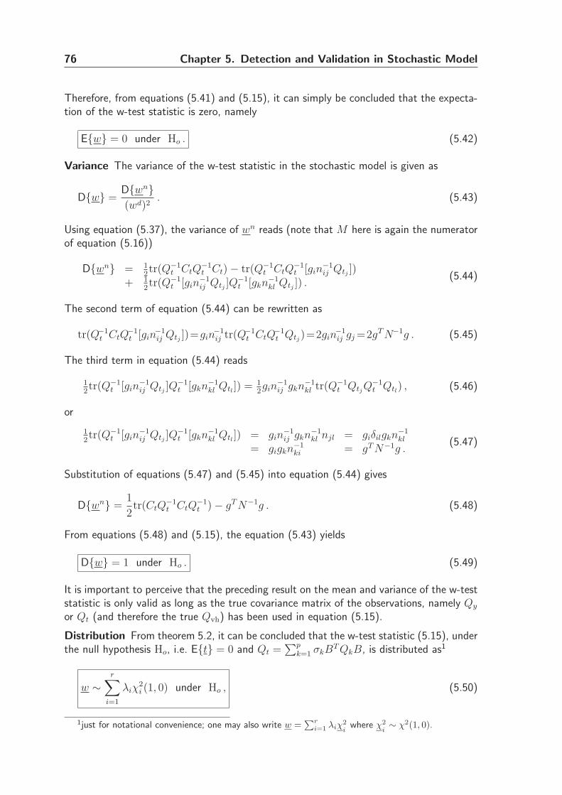
76 Chapter 5. Detection and Validation in Stochastic Model
Therefore, from equations (5.41) and (5.15), it can simply be concluded that the expecta-tion of the w-test statistic is zero, namely
E{w} = 0 under Ho . (5.42)
Variance The variance of the w-test statistic in the stochastic model is given as
D{w} =D{wn}(wd)2
. (5.43)
Using equation (5.37), the variance of wn reads (note that M here is again the numeratorof equation (5.16))
D{wn} = 12tr(Q−1
t CtQ−1t Ct)− tr(Q−1
t CtQ−1t [gin
−1ij Qtj ])
+ 12tr(Q−1
t [gin−1ij Qtj ]Q
−1t [gkn
−1kl Qtj ]) .
(5.44)
The second term of equation (5.44) can be rewritten as
tr(Q−1t CtQ
−1t [gin
−1ij Qtj ])=gin
−1ij tr(Q−1
t CtQ−1t Qtj)=2gin
−1ij gj =2gT N−1g . (5.45)
The third term in equation (5.44) reads
12tr(Q−1
t [gin−1ij Qtj ]Q
−1t [gkn
−1kl Qtl ]) = 1
2gin
−1ij gkn
−1kl tr(Q−1
t QtjQ−1t Qtl) , (5.46)
or
12tr(Q−1
t [gin−1ij Qtj ]Q
−1t [gkn
−1kl Qtl ]) = gin
−1ij gkn
−1kl njl = giδilgkn
−1kl
= gigkn−1ki = gT N−1g .
(5.47)
Substitution of equations (5.47) and (5.45) into equation (5.44) gives
D{wn} =1
2tr(CtQ
−1t CtQ
−1t )− gT N−1g . (5.48)
From equations (5.48) and (5.15), the equation (5.43) yields
D{w} = 1 under Ho . (5.49)
It is important to perceive that the preceding result on the mean and variance of the w-teststatistic is only valid as long as the true covariance matrix of the observations, namely Qy
or Qt (and therefore the true Qvh) has been used in equation (5.15).
Distribution From theorem 5.2, it can be concluded that the w-test statistic (5.15), underthe null hypothesis Ho, i.e. E{t} = 0 and Qt =
∑pk=1 σkB
T QkB, is distributed as1
w ∼r∑
i=1
λiχ2i (1, 0) under Ho , (5.50)
1just for notational convenience; one may also write w =∑r
i=1 λiχ2i
where χ2i∼ χ2(1, 0).
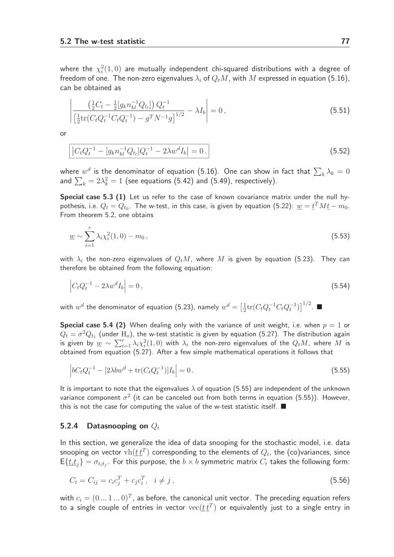
5.2 The w-test statistic 77
where the χ2i (1, 0) are mutually independent chi-squared distributions with a degree of
freedom of one. The non-zero eigenvalues λi of QtM , with M expressed in equation (5.16),can be obtained as∣∣∣∣∣
(12Ct − 1
2[gkn
−1kl Qtl ]
)Q−1
t[
12tr(CtQ
−1t CtQ
−1t )− gT N−1g
]1/2− λIb
∣∣∣∣∣= 0 , (5.51)
or
∣∣CtQ
−1t − [gkn
−1kl Qtl ]Q
−1t − 2λwdIb
∣∣ = 0 . (5.52)
where wd is the denominator of equation (5.16). One can show in fact that∑
k λk = 0and
∑
k = 2λ2k = 1 (see equations (5.42) and (5.49), respectively).
Special case 5.3 (1) Let us refer to the case of known covariance matrix under the null hy-pothesis, i.e. Qt = Qt0 . The w-test, in this case, is given by equation (5.22): w = tT Mt−m0.From theorem 5.2, one obtains
w ∼r∑
i=1
λiχ2i (1, 0)−m0 , (5.53)
with λi the non-zero eigenvalues of QtM , where M is given by equation (5.23). They cantherefore be obtained from the following equation:
∣∣∣CtQ
−1t − 2λwdIb
∣∣∣ = 0 , (5.54)
with wd the denominator of equation (5.23), namely wd =[
12tr(CtQ
−1t CtQ
−1t )]1/2
. �
Special case 5.4 (2) When dealing only with the variance of unit weight, i.e. when p = 1 orQt = σ2Qt1 (under Ho), the w-test statistic is given by equation (5.27). The distribution againis given by w ∼ ∑r
i=1 λiχ2i (1, 0) with λi the non-zero eigenvalues of the QtM , where M is
obtained from equation (5.27). After a few simple mathematical operations it follows that
∣∣∣bCtQ
−1t − [2λbwd + tr(CtQ
−1t )]Ib
∣∣∣ = 0 . (5.55)
It is important to note that the eigenvalues λ of equation (5.55) are independent of the unknownvariance component σ2 (it can be canceled out from both terms in equation (5.55)). However,this is not the case for computing the value of the w-test statistic itself. �
5.2.4 Datasnooping on Qt
In this section, we generalize the idea of data snooping for the stochastic model, i.e. datasnooping on vector vh(t tT ) corresponding to the elements of Qt, the (co)variances, sinceE{titj} = σtitj . For this purpose, the b× b symmetric matrix Ct takes the following form:
Ct = Cij = cicTj + cjc
Ti , i 6= j , (5.56)
with ci = (0 ... 1 ... 0)T , as before, the canonical unit vector. The preceding equation refersto a single couple of entries in vector vec(t tT ) or equivalently just to a single entry in
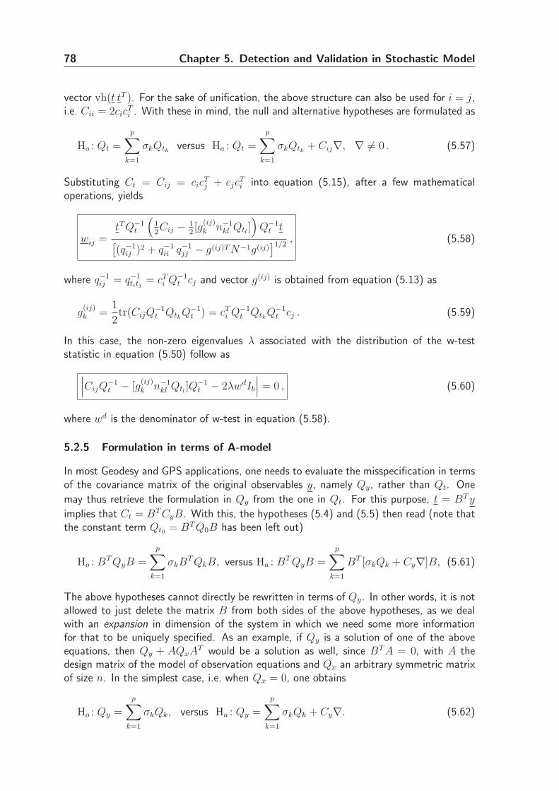
78 Chapter 5. Detection and Validation in Stochastic Model
vector vh(t tT ). For the sake of unification, the above structure can also be used for i = j,i.e. Cii = 2cic
Ti . With these in mind, the null and alternative hypotheses are formulated as
Ho : Qt =
p∑
k=1
σkQtk versus Ha : Qt =
p∑
k=1
σkQtk + Cij∇, ∇ 6= 0 . (5.57)
Substituting Ct = Cij = cicTj + cjc
Ti into equation (5.15), after a few mathematical
operations, yields
wij =tT Q−1
t
(12Cij − 1
2[g
(ij)k n−1
kl Qtl ])
Q−1t t
[(q−1
ij )2 + q−1ii q−1
jj − g(ij)T N−1g(ij)]1/2
, (5.58)
where q−1ij = q−1
titj = cTi Q−1
t cj and vector g(ij) is obtained from equation (5.13) as
g(ij)k =
1
2tr(CijQ
−1t QtkQ
−1t ) = cT
i Q−1t QtkQ
−1t cj . (5.59)
In this case, the non-zero eigenvalues λ associated with the distribution of the w-teststatistic in equation (5.50) follow as
∣∣∣CijQ
−1t − [g
(ij)k n−1
kl Qtl ]Q−1t − 2λwdIb
∣∣∣ = 0 , (5.60)
where wd is the denominator of w-test in equation (5.58).
5.2.5 Formulation in terms of A-model
In most Geodesy and GPS applications, one needs to evaluate the misspecification in termsof the covariance matrix of the original observables y, namely Qy, rather than Qt. One
may thus retrieve the formulation in Qy from the one in Qt. For this purpose, t = BT y
implies that Ct = BT CyB. With this, the hypotheses (5.4) and (5.5) then read (note thatthe constant term Qt0 = BT Q0B has been left out)
Ho : BT QyB =
p∑
k=1
σkBT QkB, versus Ha : BT QyB =
p∑
k=1
BT [σkQk + Cy∇]B, (5.61)
The above hypotheses cannot directly be rewritten in terms of Qy. In other words, it is notallowed to just delete the matrix B from both sides of the above hypotheses, as we dealwith an expansion in dimension of the system in which we need some more informationfor that to be uniquely specified. As an example, if Qy is a solution of one of the aboveequations, then Qy + AQxA
T would be a solution as well, since BT A = 0, with A thedesign matrix of the model of observation equations and Qx an arbitrary symmetric matrixof size n. In the simplest case, i.e. when Qx = 0, one obtains
Ho : Qy =
p∑
k=1
σkQk, versus Ha : Qy =
p∑
k=1
σkQk + Cy∇. (5.62)
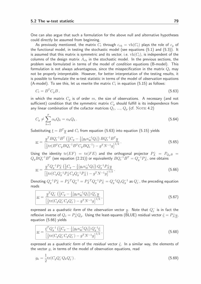
5.2 The w-test statistic 79
One can also argue that such a formulation for the above null and alternative hypothesescould directly be assumed from beginning.
As previously mentioned, the matrix Ct through cvh = vh(Ct) plays the role of cy ofthe functional model, in testing the stochastic model (see equations (5.1) and (5.3)). Itis assumed that this matrix is symmetric and its vector, i.e. vh(Ct), is independent of thecolumns of the design matrix Avh in the stochastic model. In the previous sections, theproblem was formulated in terms of the model of condition equations (B-model). Thisformulation is not always advantageous, since the misspecification in the matrix Qt maynot be properly interpretable. However, for better interpretation of the testing results, itis possible to formulate the w-test statistic in terms of the model of observation equations(A-model). To see this, let us rewrite the matrix Ct in equation (5.15) as follows:
Ct = BT CyB , (5.63)
in which the matrix Cy is of order m, the size of observations. A necessary (and notsufficient) condition that the symmetric matrix Cy should fulfill is its independence fromany linear combination of the cofactor matrices Q1, ..., Qp (cf. Note 4.2)
Cy 6=p∑
k=1
αkQk = αkQk . (5.64)
Substituting t = BT y and Ct from equation (5.63) into equation (5.15) yields
w =yT BQ−1
t BT(
12Cy − 1
2[gkn
−1kl Ql]
)BQ−1
t BT y[
12tr(BT CyBQ−1
t BT CyBQ−1t )− gT N−1g
]1/2. (5.65)
Using the identity tr(EF ) = tr(FE) and the orthogonal projector P⊥A = PQyB =
QyBQ−1t BT (see equation (2.21)) or equivalently BQ−1
t BT = Q−1y P⊥
A , one obtains
w =yT Q−1
y P⊥A
(12Cy − 1
2[gkn
−1kl Ql]
)Q−1
y P⊥A y
[12tr(CyQ−1
y P⊥A CyQ−1
y P⊥A )− gT N−1g
]1/2. (5.66)
Denoting Q−1y P⊥
A = P⊥TA Q−1
y = P⊥TA Q−1
y P⊥A = Q−1
y QeQ−1y as Q−
e , the preceding equationreads
w =yT Q−
e
(12Cy − 1
2[gkn
−1kl Ql]
)Q−
e y[
12tr(CyQ
−e CyQ
−e )− gT N−1g
]1/2, (5.67)
expressed as a quadratic form of the observation vector y. Note that Q−e is in fact the
reflexive inverse of Qe = P⊥A Qy. Using the least-squares (BLUE) residual vector e = P⊥
A y,equation (5.66) yields
w =eT Q−1
y
(12Cy − 1
2[gkn
−1kl Ql]
)Q−1
y e[
12tr(CyQ
−e CyQ
−e )− gT N−1g
]1/2, (5.68)
expressed as a quadratic form of the residual vector e. In a similar way, the elements ofthe vector g, in terms of the model of observation equations, read
gk =1
2tr(CyQ
−e QkQ
−e ) . (5.69)
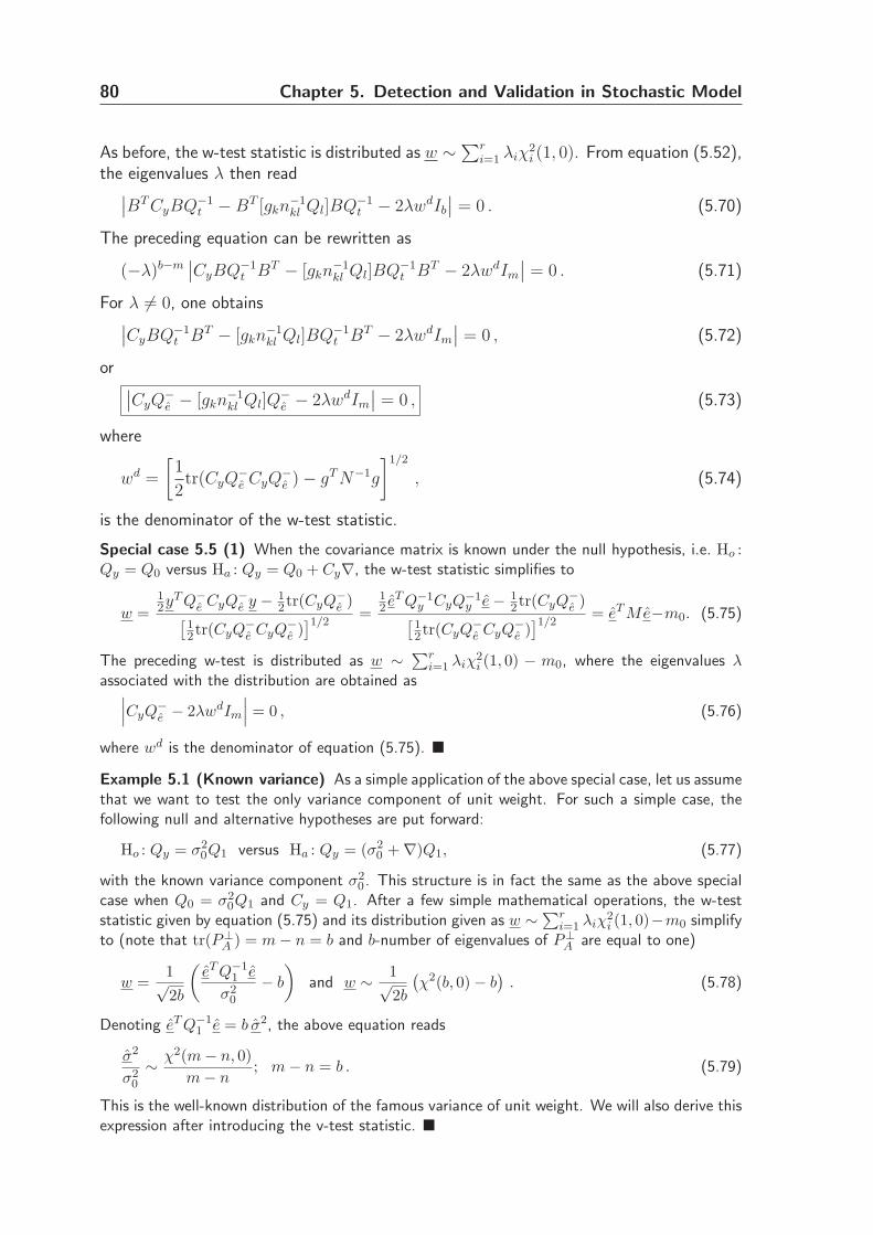
80 Chapter 5. Detection and Validation in Stochastic Model
As before, the w-test statistic is distributed as w ∼∑ri=1 λiχ
2i (1, 0). From equation (5.52),
the eigenvalues λ then read∣∣BT CyBQ−1
t −BT [gkn−1kl Ql]BQ−1
t − 2λwdIb
∣∣ = 0 . (5.70)
The preceding equation can be rewritten as
(−λ)b−m∣∣CyBQ−1
t BT − [gkn−1kl Ql]BQ−1
t BT − 2λwdIm
∣∣ = 0 . (5.71)
For λ 6= 0, one obtains∣∣CyBQ−1
t BT − [gkn−1kl Ql]BQ−1
t BT − 2λwdIm
∣∣ = 0 , (5.72)
or∣∣CyQ
−e − [gkn
−1kl Ql]Q
−e − 2λwdIm
∣∣ = 0 , (5.73)
where
wd =
[1
2tr(CyQ
−e CyQ
−e )− gT N−1g
]1/2
, (5.74)
is the denominator of the w-test statistic.
Special case 5.5 (1) When the covariance matrix is known under the null hypothesis, i.e. Ho :Qy = Q0 versus Ha : Qy = Q0 + Cy∇, the w-test statistic simplifies to
w =12yT Q−
e CyQ−e y − 1
2tr(CyQ−e )
[12tr(CyQ
−e CyQ
−e )]1/2
=12 eT Q−1
y CyQ−1y e− 1
2tr(CyQ−e )
[12tr(CyQ
−e CyQ
−e )]1/2
= eT Me−m0. (5.75)
The preceding w-test is distributed as w ∼ ∑ri=1 λiχ
2i (1, 0) − m0, where the eigenvalues λ
associated with the distribution are obtained as∣∣∣CyQ
−e − 2λwdIm
∣∣∣ = 0 , (5.76)
where wd is the denominator of equation (5.75). �
Example 5.1 (Known variance) As a simple application of the above special case, let us assumethat we want to test the only variance component of unit weight. For such a simple case, thefollowing null and alternative hypotheses are put forward:
Ho : Qy = σ20Q1 versus Ha : Qy = (σ2
0 +∇)Q1, (5.77)
with the known variance component σ20. This structure is in fact the same as the above special
case when Q0 = σ20Q1 and Cy = Q1. After a few simple mathematical operations, the w-test
statistic given by equation (5.75) and its distribution given as w ∼∑ri=1 λiχ
2i (1, 0)−m0 simplify
to (note that tr(P⊥A ) = m− n = b and b-number of eigenvalues of P⊥
A are equal to one)
w =1√2b
(eT Q−1
1 e
σ20
− b
)
and w ∼ 1√2b
(χ2(b, 0)− b
). (5.78)
Denoting eT Q−11 e = b σ2, the above equation reads
σ2
σ20
∼ χ2(m− n, 0)
m− n; m− n = b . (5.79)
This is the well-known distribution of the famous variance of unit weight. We will also derive thisexpression after introducing the v-test statistic. �
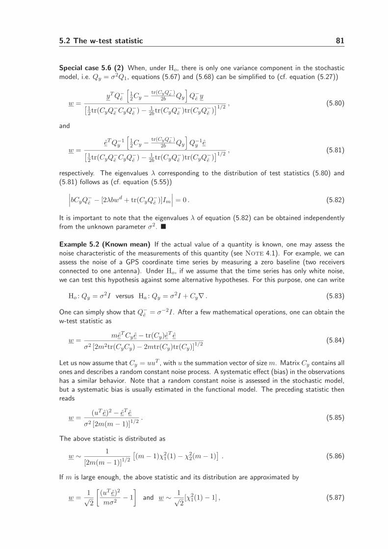
5.2 The w-test statistic 81
Special case 5.6 (2) When, under Ho, there is only one variance component in the stochasticmodel, i.e. Qy = σ2Q1, equations (5.67) and (5.68) can be simplified to (cf. equation (5.27))
w =yT Q−
e
[12Cy − tr(CyQ−
e)
2b Qy
]
Q−e y
[12tr(CyQ
−e CyQ
−e )− 1
2btr(CyQ−e )tr(CyQ
−e )]1/2
, (5.80)
and
w =eT Q−1
y
[12Cy − tr(CyQ−
e)
2b Qy
]
Q−1y e
[12tr(CyQ
−e CyQ
−e )− 1
2btr(CyQ−e )tr(CyQ
−e )]1/2
, (5.81)
respectively. The eigenvalues λ corresponding to the distribution of test statistics (5.80) and(5.81) follows as (cf. equation (5.55))
∣∣∣bCyQ
−e − [2λbwd + tr(CyQ
−e )]Im
∣∣∣ = 0 . (5.82)
It is important to note that the eigenvalues λ of equation (5.82) can be obtained independentlyfrom the unknown parameter σ2. �
Example 5.2 (Known mean) If the actual value of a quantity is known, one may assess thenoise characteristic of the measurements of this quantity (see Note 4.1). For example, we canassess the noise of a GPS coordinate time series by measuring a zero baseline (two receiversconnected to one antenna). Under Ho, if we assume that the time series has only white noise,we can test this hypothesis against some alternative hypotheses. For this purpose, one can write
Ho : Qy = σ2I versus Ha : Qy = σ2I + Cy∇ . (5.83)
One can simply show that Q−e = σ−2I. After a few mathematical operations, one can obtain the
w-test statistic as
w =meT Cy e− tr(Cy)e
T e
σ2 [2m2tr(CyCy)− 2mtr(Cy)tr(Cy)]1/2
(5.84)
Let us now assume that Cy = uuT , with u the summation vector of size m. Matrix Cy contains allones and describes a random constant noise process. A systematic effect (bias) in the observationshas a similar behavior. Note that a random constant noise is assessed in the stochastic model,but a systematic bias is usually estimated in the functional model. The preceding statistic thenreads
w =(uT e)2 − eT e
σ2 [2m(m− 1)]1/2. (5.85)
The above statistic is distributed as
w ∼ 1
[2m(m− 1)]1/2
[(m− 1)χ2
1(1)− χ22(m− 1)
]. (5.86)
If m is large enough, the above statistic and its distribution are approximated by
w =1√2
[(uT e)2
mσ2− 1
]
and w ∼ 1√2[χ2
1(1)− 1] , (5.87)

82 Chapter 5. Detection and Validation in Stochastic Model
which yields
(uT e)2
mσ2∼ χ2
1(1) oruT e√mσ∼ N(0, 1) . (5.88)
The preceding formula could directly be obtained from the functional model when we includean unknown bias term, namely bx, in the functional model. In this case, its least-squares solutionreads bx = uT e/m. When testing the hypothesis Ho : bx = 0 versus Ha : bx 6= 0 (parametersignificance test, see section 2.2.5), the same formula as above can be obtained. �
5.2.6 Datasnooping on Qy
As with the datasnooping on the elements of the vector vh(t tT ) or correspondingly on theelements of Qt, suggested in section 5.2.4, one can also apply this idea to the elements ofQy, the variances and covariances of the observables. In this case, the m×m symmetricmatrix Cy takes the form
Cy = Cij = cicTj + cjc
Ti , i, j = 1, 2, ...,m, , (5.89)
with ci and cj the canonical unit vectors of length m, referring to a single couple of entriesin matrix Qy, the ijth and jith element, the (co)variances. Taking the above form for thematrix Cy, the null and alternative hypotheses read
Ho : Qy =
p∑
k=1
σkQk versus Ha : Qy =
p∑
k=1
σkQk + Cij∇, ∇ 6= 0 . (5.90)
Substituting Cy from equation (5.89) into equation (5.67) gives
w =yT Q−
e
(12Cij − 1
2[gkn
−1kl Ql]
)Q−
e y[(q−ij)
2 + q−ii q−jj − g(ij)T N−1g(ij)
]1/2, (5.91)
with q−ij = ciQ−e cj. The p-vector g(ij) follows from equation (5.69): g
(ij)k = cT
i Q−e QkQ
−e cj
(substitute Cy from equation (5.89)). The eigenvalues associated with the distribution ofthe preceding w-test statistic follow from equation (5.73)∣∣CijQ
−e − [gkn
−1kl Ql]Q
−e − 2λwdIm
∣∣ = 0 (5.92)
with wd the denominator of equation (5.91). In terms of the least-squares residuals e =P⊥
A y, a similar formulation can be given for the w-test statistic.
Special case 5.7 (1) In the case that the covariance matrix is known, i.e. Ho : Qy = Q0 versusHa : Qy = Q0 + Cij∇, the w-test statistic (5.75) reads
w =12yT Q−
e CijQ−e y − q−ij
[
(q−ij)2 + q−ii q
−jj
]1/2=
12 eT Q−1
y CijQ−1y e− q−ij
[
(q−ij)2 + q−ii q
−jj
]1/2= eT Me−m0. (5.93)
This test statistic is again distributed as w ∼ λkχ2k(1, 0)−m0, where the r number of eigenvalues
λ follow from∣∣∣CijQ
−e − 2λwdIm
∣∣∣ = 0 , (5.94)
where wd is the denominator of equation (5.93). �
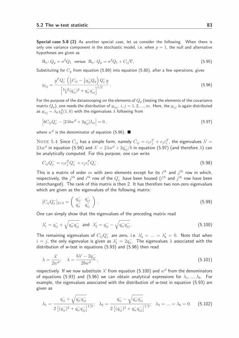
5.2 The w-test statistic 83
Special case 5.8 (2) As another special case, let us consider the following. When there isonly one variance component in the stochastic model, i.e. when p = 1, the null and alternativehypotheses are given as
Ho : Qy = σ2Q1 versus Ha : Qy = σ2Q1 + Cij∇, (5.95)
Substituting for Cy from equation (5.89) into equation (5.80), after a few operations, gives
wij =yT Q−
e
(12Cij − 1
b q−ijQy
)
Q−e y
[b−2
b (q−ij)2 + q−ii q
−jj
]1/2. (5.96)
For the purpose of the datasnooping on the elements of Qy (testing the elements of the covariancematrix Qy), one needs the distribution of wij , i, j = 1, 2, ..., m. Here, the wij is again distributedas wij ∼ λkχ
2k(1, 0) with the eigenvalues λ following from
∣∣∣bCijQ
−e − [2λbwd + 2q−ij ]Im
∣∣∣ = 0 , (5.97)
where wd is the denominator of equation (5.96). �
Note 5.4 Since Cij has a simple form, namely Cij = cicTj + cjc
Ti , the eigenvalues λ′ =
2λwd in equation (5.94) and λ′ = 2λwd + 2q−ij/b in equation (5.97) (and therefore λ) canbe analytically computed. For this purpose, one can write
CijQ−e = cic
Tj Q−
e + cjcTi Q−
e . (5.98)
This is a matrix of order m with zero elements except for its ith and jth row in which,respectively, the jth and ith row of the Q−
e have been housed (ith and jth row have beeninterchanged). The rank of this matrix is then 2. It has therefore two non-zero eigenvalueswhich are given as the eigenvalues of the following matrix:
[CijQ−e ]2×2 =
(q−ij q−jjq−ii q−ij
)
. (5.99)
One can simply show that the eigenvalues of the preceding matrix read
λ′1 = q−ij +
√
q−ii q−jj and λ′
2 = q−ij −√
q−ii q−jj . (5.100)
The remaining eigenvalues of CijQ−e are zero, i.e. λ′
3 = ... = λ′b = 0. Note that when
i = j, the only eigenvalue is given as λ′1 = 2q−ii . The eigenvalues λ associated with the
distribution of w-test in equations (5.93) and (5.96) then read
λ =λ′
2wd; λ =
bλ′ − 2q−ij2bwd
, (5.101)
respectively. If we now substitute λ′ from equation (5.100) and wd from the denominatorsof equations (5.93) and (5.96) we can obtain analytical expressions for λ1, ..., λb. Forexample, the eigenvalues associated with the distribution of w-test in equation (5.93) aregiven as
λ1 =q−ij +
√
q−ii q−jj
2[(q−ij)
2 + q−ii q−jj
]1/2; λ2 =
q−ij −√
q−ii q−jj
2[(q−ij)
2 + q−ii q−jj
]1/2; λ3 = ... = λb = 0. (5.102)
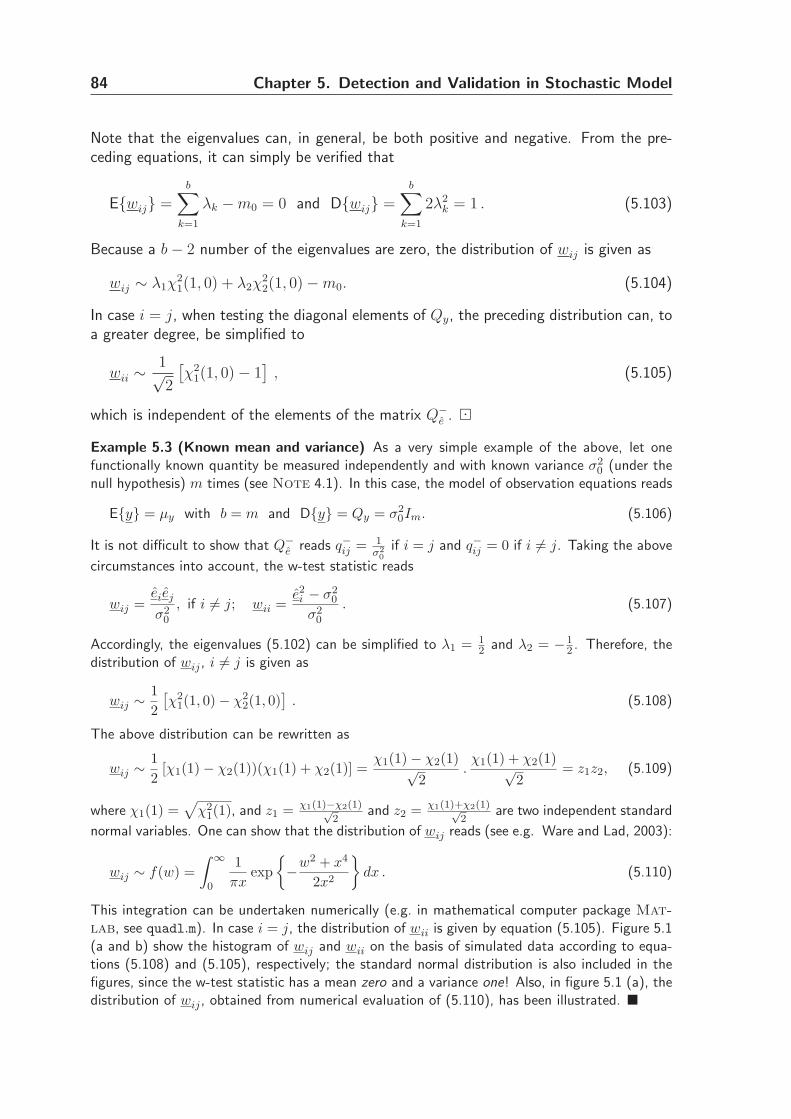
84 Chapter 5. Detection and Validation in Stochastic Model
Note that the eigenvalues can, in general, be both positive and negative. From the pre-ceding equations, it can simply be verified that
E{wij} =b∑
k=1
λk −m0 = 0 and D{wij} =b∑
k=1
2λ2k = 1 . (5.103)
Because a b− 2 number of the eigenvalues are zero, the distribution of wij is given as
wij ∼ λ1χ21(1, 0) + λ2χ
22(1, 0)−m0. (5.104)
In case i = j, when testing the diagonal elements of Qy, the preceding distribution can, toa greater degree, be simplified to
wii ∼1√2
[χ2
1(1, 0)− 1]
, (5.105)
which is independent of the elements of the matrix Q−e . ⊡
Example 5.3 (Known mean and variance) As a very simple example of the above, let onefunctionally known quantity be measured independently and with known variance σ2
0 (under thenull hypothesis) m times (see Note 4.1). In this case, the model of observation equations reads
E{y} = µy with b = m and D{y} = Qy = σ20Im. (5.106)
It is not difficult to show that Q−e reads q−ij = 1
σ20
if i = j and q−ij = 0 if i 6= j. Taking the above
circumstances into account, the w-test statistic reads
wij =eiej
σ20
, if i 6= j; wii =e2i − σ2
0
σ20
. (5.107)
Accordingly, the eigenvalues (5.102) can be simplified to λ1 = 12 and λ2 = −1
2 . Therefore, thedistribution of wij , i 6= j is given as
wij ∼1
2
[χ2
1(1, 0)− χ22(1, 0)
]. (5.108)
The above distribution can be rewritten as
wij ∼1
2[χ1(1)− χ2(1))(χ1(1) + χ2(1)] =
χ1(1)− χ2(1)√2
.χ1(1) + χ2(1)√
2= z1z2, (5.109)
where χ1(1) =√
χ21(1), and z1 = χ1(1)−χ2(1)√
2and z2 = χ1(1)+χ2(1)√
2are two independent standard
normal variables. One can show that the distribution of wij reads (see e.g. Ware and Lad, 2003):
wij ∼ f(w) =
∫ ∞
0
1
πxexp
{
−w2 + x4
2x2
}
dx . (5.110)
This integration can be undertaken numerically (e.g. in mathematical computer package Mat-lab, see quadl.m). In case i = j, the distribution of wii is given by equation (5.105). Figure 5.1(a and b) show the histogram of wij and wii on the basis of simulated data according to equa-tions (5.108) and (5.105), respectively; the standard normal distribution is also included in thefigures, since the w-test statistic has a mean zero and a variance one! Also, in figure 5.1 (a), thedistribution of wij , obtained from numerical evaluation of (5.110), has been illustrated. �
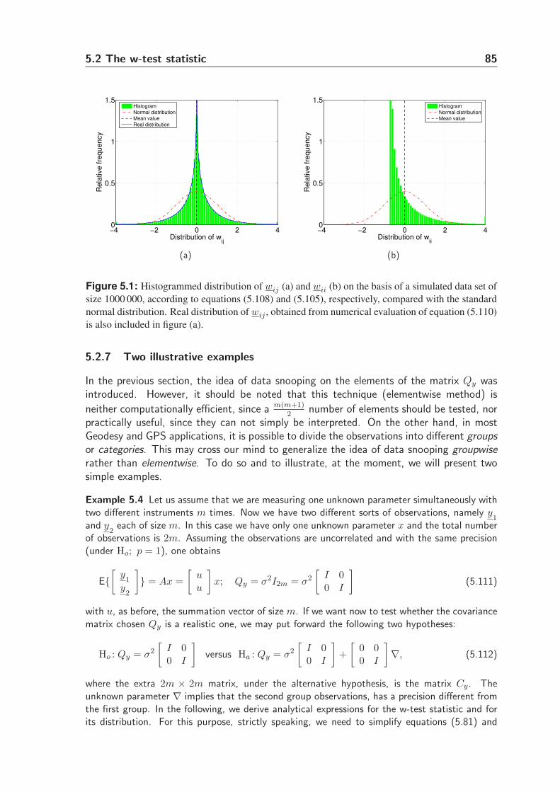
5.2 The w-test statistic 85
−4 −2 0 2 40
0.5
1
1.5
Distribution of wij
Rela
tive fre
quency
Histogram
Normal distribution
Mean value
Real distribution
(a)
−4 −2 0 2 40
0.5
1
1.5
Distribution of wii
Rela
tive fre
quency
Histogram
Normal distribution
Mean value
(b)
Figure 5.1: Histogrammed distribution of wij (a) and wii (b) on the basis of a simulated data set of
size 1000 000, according to equations (5.108) and (5.105), respectively, compared with the standard
normal distribution. Real distribution of wij , obtained from numerical evaluation of equation (5.110)
is also included in figure (a).
5.2.7 Two illustrative examples
In the previous section, the idea of data snooping on the elements of the matrix Qy wasintroduced. However, it should be noted that this technique (elementwise method) is
neither computationally efficient, since a m(m+1)2
number of elements should be tested, norpractically useful, since they can not simply be interpreted. On the other hand, in mostGeodesy and GPS applications, it is possible to divide the observations into different groupsor categories. This may cross our mind to generalize the idea of data snooping groupwiserather than elementwise. To do so and to illustrate, at the moment, we will present twosimple examples.
Example 5.4 Let us assume that we are measuring one unknown parameter simultaneously withtwo different instruments m times. Now we have two different sorts of observations, namely y
1and y
2each of size m. In this case we have only one unknown parameter x and the total number
of observations is 2m. Assuming the observations are uncorrelated and with the same precision(under Ho; p = 1), one obtains
E{[
y1
y2
]
} = Ax =
[uu
]
x; Qy = σ2I2m = σ2
[I 00 I
]
(5.111)
with u, as before, the summation vector of size m. If we want now to test whether the covariancematrix chosen Qy is a realistic one, we may put forward the following two hypotheses:
Ho : Qy = σ2
[I 00 I
]
versus Ha : Qy = σ2
[I 00 I
]
+
[0 00 I
]
∇, (5.112)
where the extra 2m × 2m matrix, under the alternative hypothesis, is the matrix Cy. Theunknown parameter ∇ implies that the second group observations, has a precision different fromthe first group. In the following, we derive analytical expressions for the w-test statistic and forits distribution. For this purpose, strictly speaking, we need to simplify equations (5.81) and
86 Chapter 5. Detection and Validation in Stochastic Model
(5.82), respectively. The w-test statistic simplifies to
w =eT2 e2 − eT
1 e1
2σ2√
m− 1, (5.113)
with e1 and e2 the least squares residual vectors of the first and second group of observations,under Ho, respectively.
Proof. The entries of matrix Q−e = Q−1
y P⊥A , of order 2m, are given as q−ij = 2m−1
2mσ2 if i = j and
q−ij = −12mσ2 if i 6= j. After a few mathematical operations, one obtains
tr(CyQ−e ) =
2m− 1
2σ2, tr(CyQ
−e CyQ
−e ) =
4m− 3
4σ4(5.114)
from which wd in equation (5.81) follows as wd =√
m−12σ2 . The terms in the numerator of
equation (5.81) simplify to
eT Q−1y CyQ
−1y e =
eT2 e2
σ4, eT Q−1
y e =eT1 e1 + eT
2 e2
σ2(5.115)
Substituting the preceding terms in equation (5.81) completes the proof. H
Note that the σ2 is unknown even under the null hypothesis. In practice, one has to be satisfied
with a least-squares estimate of this variance component, namely σ2 =eT1 e1+eT
2 e2
2m−1 . If e1 and e2
are of similar magnitude, the preceding test statistic intuitively says that the w-test value is notvery large, and therefore the null hypothesis is likely to be accepted. One will then obtain ∇ ≈ 0and therefore σ2
1 ≈ σ22.
The w-test statistic is distributed as w ∼ λkχ2k(1, 0), where the eigenvalues λ are obtained
from equation (5.82). After not very long derivations, the eigenvalues λ are given, independentof the unknown variance component σ2, as (see appendix B.1)
λ1 = 0; λ2 = ... = λm =1
2√
m− 1; λm+1 = ... = λ2m−1 =
−1
2√
m− 1, (5.116)
from which it can simply be concluded that the w-test statistic (5.113) is distributed as
w ∼ 1
2√
m− 1
[χ2
1(m− 1, 0)− χ22(m− 1, 0)
](5.117)
where χ21(m− 1, 0) and χ2
2(m− 1, 0) are two independent chi-squared distributions with m− 1degrees of freedom. One can simply show that the above distribution has a mean of zero and avariance of one. Based on the central limit theorem for independent and identically distributeddata, when m is large enough, one can approximate the chi-squared distribution by a normal one,i.e. χ2
1(m−1, 0) ≈ N(m−1, 2(m−1)). Taking these into account, one can simply show that thepreceding distribution is approximated by the standard normal distribution, namely w ≃ N(0, 1).To show this, one needs to use the following identity:
α1N1(µ1, σ21) + α2N2(µ2, σ
22) = N(α1µ1 + α2µ2, α
21σ
21 + α2
2σ22) , (5.118)
for two independent normal distributions N1 and N2, and α1 and α2 two real numbers. �
Example 5.5 In previous example, if one wants to test whether the first group of observations isindependent of the second group, one may write the null and alternative hypotheses as follows:
Ho : Qy = σ2
[I 00 I
]
versus Ha : Qy = σ2
[I 00 I
]
+
[0 II 0
]
︸ ︷︷ ︸
Cy
∇, (5.119)
5.2 The w-test statistic 87
where∇ here is a covariance component. In the following, we give formulas for the w-test statisticand its distribution. After a few mathematical and matrix operations, one can show that (seeappendix B)
w =(e2 − e1)
T (e2 − e1) + 4meT1 e2
2σ2√
2m(2m− 1)(m− 1), (5.120)
where e1 and e2 are, again, the least squares residuals of the first and second group of observations.
Proof. After a few mathematical and matrix operations, one can show that
tr(CyQ−e ) =
−1
σ2, tr(CyQ
−e CyQ
−e ) =
2m− 1
σ41
(5.121)
which yields wd = 1σ2
√2m(m−1)
2m−1 in equation (5.81). The terms in the numerator of equa-
tion (5.81) then read
eT Q−1y CyQ
−1y e =
2 eT1 e2
σ41
, eT Q−1y e =
eT1 e1 + eT
2 e2
σ2(5.122)
Substituting the preceding terms in equation (5.81) completes the proof. H
If e1 and e2 have similar corresponding values, then the term eT1 e2 in the preceding equation
becomes large, and therefore the null hypothesis is likely to be rejected. This implies that thefirst and the second observation groups are likely to be correlated.
To see how the distribution looks like, we need the eigenvalues λ from equation (5.82). We canshow that such non-zero eigenvalues (a 2m− 1 number) can be obtained as (see appendix B.2)
λ1 = ... = λm = − m−1√2m(2m−1)(m−1)
;
λm+1 = ... = λ2m−1 = m√2m(2m−1)(m−1)
.(5.123)
With these in mind, the distribution of the w-test statistic, namely λkχ2k(1, 0), simplifies to
w ∼ 1√
2m(2m− 1)(m− 1)
[mχ2
1(m− 1, 0)− (m− 1)χ22(m, 0)
], (5.124)
where χ21(m− 1, 0) and χ2
2(m, 0) are two independent chi-squared distributions with m− 1 andm degrees of freedom, respectively. One can again show that the preceding distribution hasmean zero and variance one. If m is large enough, again, the chi-squared distributions can beapproximated by normal ones. Therefore, using identity (5.118), the above distribution can beapproximated by the standard normal distribution, i.e. w ≃ N(0, 1). �
Figure (5.2), a and b, respectively, show the histogram distribution of w-test statisticpresented in formulae (5.117) and (5.124), in case of m = 50 and on the basis of a simulateddata set of size 100,000. For a visual comparison with normality, the standard normaldistribution has been plotted on the histograms. In addition, figure 5.2, c and d, illustratethe normal probability plot for the aforementioned (simulated) data sets. The normalprobability plot is a graphical technique to assess whether or not a data set is approximatelynormally distributed. The data is plotted against a theoretical normal distribution in sucha way that the points should form a straight line. Departures from this straight lineindicate departures from normality. These plots may seem curved at the ends (tails) ofthe distribution function. However, this minor curvature seems to be not significant atα = 0.05 or even α = 0.01 significance level tests.
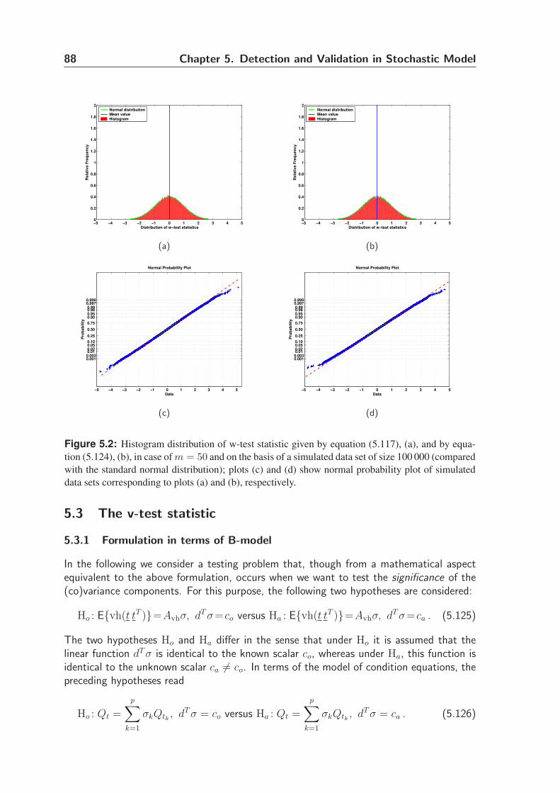
88 Chapter 5. Detection and Validation in Stochastic Model
−5 −4 −3 −2 −1 0 1 2 3 4 50
0.2
0.4
0.6
0.8
1
1.2
1.4
1.6
1.8
2
Distribution of w−test statistics
Re
lati
ve
Fre
qu
en
cy
Normal distributionMean valueHistogram
(a)
−5 −4 −3 −2 −1 0 1 2 3 4 50
0.2
0.4
0.6
0.8
1
1.2
1.4
1.6
1.8
2
Distribution of w−test statistics
Re
lati
ve
Fre
qu
en
cy
Normal distributionMean valueHistogram
(b)
−5 −4 −3 −2 −1 0 1 2 3 4 5
0.0010.0030.01 0.02 0.05 0.10
0.25
0.50
0.75
0.90 0.95 0.98 0.99
0.9970.999
Data
Pro
ba
bil
ity
Normal Probability Plot
(c)
−5 −4 −3 −2 −1 0 1 2 3 4 5
0.0010.0030.01 0.02 0.05 0.10
0.25
0.50
0.75
0.90 0.95 0.98 0.99
0.9970.999
Data
Pro
ba
bil
ity
Normal Probability Plot
(d)
Figure 5.2: Histogram distribution of w-test statistic given by equation (5.117), (a), and by equa-
tion (5.124), (b), in case of m = 50 and on the basis of a simulated data set of size 100 000 (compared
with the standard normal distribution); plots (c) and (d) show normal probability plot of simulated
data sets corresponding to plots (a) and (b), respectively.
5.3 The v-test statistic
5.3.1 Formulation in terms of B-model
In the following we consider a testing problem that, though from a mathematical aspectequivalent to the above formulation, occurs when we want to test the significance of the(co)variance components. For this purpose, the following two hypotheses are considered:
Ho : E{vh(t tT )}=Avhσ, dT σ=co versus Ha : E{vh(t tT )}=Avhσ, dT σ=ca . (5.125)
The two hypotheses Ho and Ha differ in the sense that under Ho it is assumed that thelinear function dT σ is identical to the known scalar co, whereas under Ha, this function isidentical to the unknown scalar ca 6= co. In terms of the model of condition equations, thepreceding hypotheses read
Ho : Qt =
p∑
k=1
σkQtk , dT σ = co versus Ha : Qt =
p∑
k=1
σkQtk , dT σ = ca . (5.126)
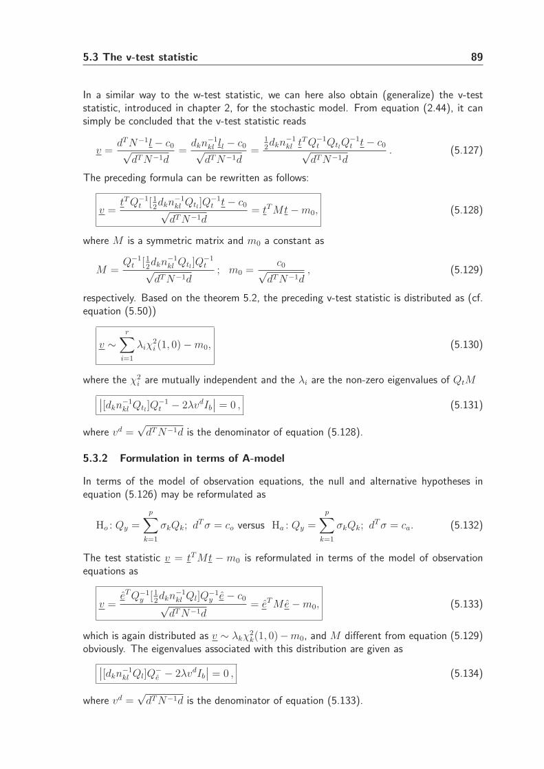
5.3 The v-test statistic 89
In a similar way to the w-test statistic, we can here also obtain (generalize) the v-teststatistic, introduced in chapter 2, for the stochastic model. From equation (2.44), it cansimply be concluded that the v-test statistic reads
v =dT N−1l − c0√
dT N−1d=
dkn−1kl ll − c0√dT N−1d
=12dkn
−1kl tT Q−1
t QtlQ−1t t− c0√
dT N−1d. (5.127)
The preceding formula can be rewritten as follows:
v =tT Q−1
t [12dkn
−1kl Qtl ]Q
−1t t− c0√
dT N−1d= tT Mt−m0, (5.128)
where M is a symmetric matrix and m0 a constant as
M =Q−1
t [12dkn
−1kl Qtl ]Q
−1t√
dT N−1d; m0 =
c0√dT N−1d
, (5.129)
respectively. Based on the theorem 5.2, the preceding v-test statistic is distributed as (cf.equation (5.50))
v ∼r∑
i=1
λiχ2i (1, 0)−m0, (5.130)
where the χ2i are mutually independent and the λi are the non-zero eigenvalues of QtM
∣∣[dkn
−1kl Qtl ]Q
−1t − 2λvdIb
∣∣ = 0 , (5.131)
where vd =√
dT N−1d is the denominator of equation (5.128).
5.3.2 Formulation in terms of A-model
In terms of the model of observation equations, the null and alternative hypotheses inequation (5.126) may be reformulated as
Ho : Qy =
p∑
k=1
σkQk; dT σ = co versus Ha : Qy =
p∑
k=1
σkQk; dT σ = ca. (5.132)
The test statistic v = tT Mt − m0 is reformulated in terms of the model of observationequations as
v =eT Q−1
y [12dkn
−1kl Ql]Q
−1y e− c0√
dT N−1d= eT Me−m0, (5.133)
which is again distributed as v ∼ λkχ2k(1, 0)−m0, and M different from equation (5.129)
obviously. The eigenvalues associated with this distribution are given as
∣∣[dkn
−1kl Ql]Q
−e − 2λvdIb
∣∣ = 0 , (5.134)
where vd =√
dT N−1d is the denominator of equation (5.133).
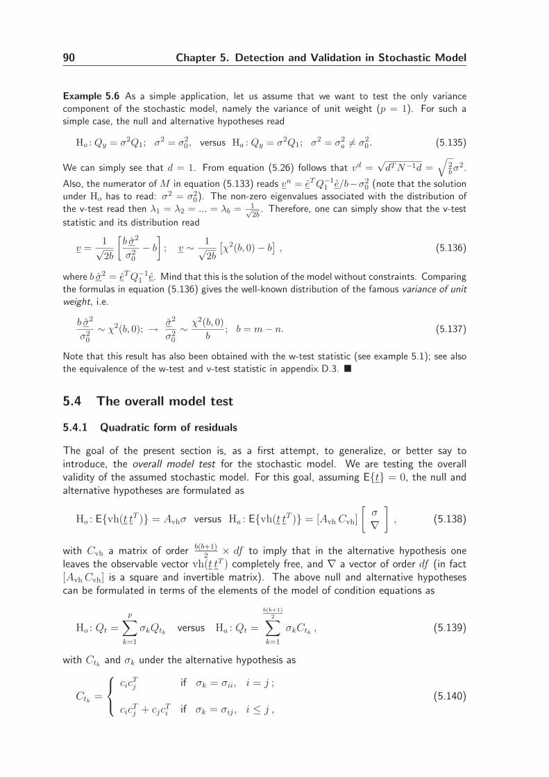
90 Chapter 5. Detection and Validation in Stochastic Model
Example 5.6 As a simple application, let us assume that we want to test the only variancecomponent of the stochastic model, namely the variance of unit weight (p = 1). For such asimple case, the null and alternative hypotheses read
Ho : Qy = σ2Q1; σ2 = σ20, versus Ha : Qy = σ2Q1; σ2 = σ2
a 6= σ20. (5.135)
We can simply see that d = 1. From equation (5.26) follows that vd =√
dT N−1d =√
2bσ
2.
Also, the numerator of M in equation (5.133) reads vn = eT Q−11 e/b−σ2
0 (note that the solutionunder Ho has to read: σ2 = σ2
0). The non-zero eigenvalues associated with the distribution ofthe v-test read then λ1 = λ2 = ... = λb = 1√
2b. Therefore, one can simply show that the v-test
statistic and its distribution read
v =1√2b
[b σ2
σ20
− b
]
; v ∼ 1√2b
[χ2(b, 0)− b
], (5.136)
where b σ2 = eT Q−11 e. Mind that this is the solution of the model without constraints. Comparing
the formulas in equation (5.136) gives the well-known distribution of the famous variance of unitweight, i.e.
b σ2
σ20
∼ χ2(b, 0); → σ2
σ20
∼ χ2(b, 0)
b; b = m− n. (5.137)
Note that this result has also been obtained with the w-test statistic (see example 5.1); see alsothe equivalence of the w-test and v-test statistic in appendix D.3. �
5.4 The overall model test
5.4.1 Quadratic form of residuals
The goal of the present section is, as a first attempt, to generalize, or better say tointroduce, the overall model test for the stochastic model. We are testing the overallvalidity of the assumed stochastic model. For this goal, assuming E{t} = 0, the null andalternative hypotheses are formulated as
Ho : E{vh(t tT )} = Avhσ versus Ha : E{vh(t tT )} = [Avh Cvh]
[σ∇
]
, (5.138)
with Cvh a matrix of order b(b+1)2× df to imply that in the alternative hypothesis one
leaves the observable vector vh(t tT ) completely free, and ∇ a vector of order df (in fact[Avh Cvh] is a square and invertible matrix). The above null and alternative hypothesescan be formulated in terms of the elements of the model of condition equations as
Ho : Qt =
p∑
k=1
σkQtk versus Ha : Qt =
b(b+1)2∑
k=1
σkCtk , (5.139)
with Ctk and σk under the alternative hypothesis as
Ctk =
cicTj if σk = σii, i = j ;
cicTj + cjc
Ti if σk = σij, i ≤ j ,
(5.140)
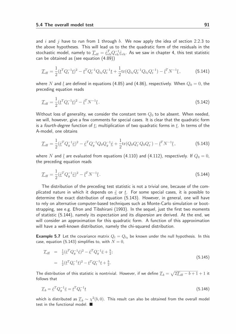
5.4 The overall model test 91
and i and j have to run from 1 through b. We now apply the idea of section 2.2.3 tothe above hypotheses. This will lead us to the the quadratic form of the residuals in thestochastic model, namely to T df = eT
vhQ−1vh evh. As we saw in chapter 4, this test statistic
can be obtained as (see equation (4.89))
T df =1
2(tT Q−1
t t)2 − tT Q−1t Qt0Q
−1t t +
1
2tr(Qt0Q
−1t Qt0Q
−1t )− lT N−1l , (5.141)
where N and l are defined in equations (4.85) and (4.86), respectively. When Q0 = 0, thepreceding equation reads
T df =1
2(tT Q−1
t t)2 − lT N−1l . (5.142)
Without loss of generality, we consider the constant term Q0 to be absent. When needed,we will, however, give a few comments for special cases. It is clear that the quadratic formis a fourth-degree function of t; multiplication of two quadratic forms in t. In terms of theA-model, one obtains
T df =1
2(eT Q−1
y e)2 − eT Q−1y Q0Q
−1y e +
1
2tr(Q0Q
−e Q0Q
−e )− lT N−1l , (5.143)
where N and l are evaluated from equations (4.110) and (4.112), respectively. If Q0 = 0,the preceding equation reads
T df =1
2(eT Q−1
y e)2 − lT N−1l . (5.144)
The distribution of the preceding test statistic is not a trivial one, because of the com-plicated nature in which it depends on e or t. For some special cases, it is possible todetermine the exact distribution of equation (5.143). However, in general, one will haveto rely on alternative computer-based techniques such as Monte-Carlo simulation or boot-strapping, see e.g. Efron and Tibshirani (1993). In the sequel, just the first two momentsof statistic (5.144), namely its expectation and its dispersion are derived. At the end, wewill consider an approximation for this quadratic form. A function of this approximationwill have a well-known distribution, namely the chi-squared distribution.
Example 5.7 Let the covariance matrix Qt = Qt0 be known under the null hypothesis. In thiscase, equation (5.143) simplifies to, with N = 0,
T df = 12(eT Q−1
y e)2 − eT Q−1y e + b
2 ;
= 12(tT Q−1
t t)2 − tT Q−1t t + b
2 .
(5.145)
The distribution of this statistic is nontrivial. However, if we define T b =√
2T df − b + 1 + 1 itfollows that
T b = eT Q−1y e = tT Q−1
t t (5.146)
which is distributed as T b ∼ χ2(b, 0). This result can also be obtained from the overall modeltest in the functional model. �
92 Chapter 5. Detection and Validation in Stochastic Model
5.4.2 Expectation of quadratic form
The usual assumption, from now on, is that the b × 1 misclosure vector t is normallydistributed, i.e. t ∼ N(0, Qt). From equation (C.37), one obtains
E{12(tT Q−1
t t)2} =1
2E{(tT Q−1
t t)(tT Q−1t t)} =
1
2b(b + 2) . (5.147)
The expectation of the second term in equation (5.142) reads
E{lT N−1l} = E{tr(lT N−1l)} = E{tr(N−1l lT )} = tr(N−1E{l lT}) , (5.148)
where matrix E{l lT} is given as (see equation (4.86))
E{l lT} = E{lilj} =1
4E{(tT
A︷ ︸︸ ︷
Q−1t QtiQ
−1t t)(tT
B︷ ︸︸ ︷
Q−1t QtjQ
−1t t)} , (5.149)
with A and B temporary matrices as in equation (C.33). One then obtains
E{l lT} = 14tr(Q−1
t Qti)tr(Q−1t Qtj) + 1
2tr(Q−1
t QtiQ−1t Qtj)
= lilj + nij = l lT + N ,(5.150)
with li = 12tr(Q−1
t Qti), the expectation of li. Substitution of the preceding equation inequation (5.148) yields
E{lT N−1l} = tr(N−1[llT + N ]) = p + lT N−1l . (5.151)
The term lT N−1l in the preceding formulas can be simplified to
lT N−1l = lT σ = liσi =1
2tr(Q−1
t Qti)σi =1
2tr(Q−1
t [σiQti ]) =b
2. (5.152)
Taking the expectation of equation (5.142) and substituting the first and second termsfrom equations (5.147) and (5.151), respectively, under null-hypothesis Ho, result in theexpectation of the quadratic form as the redundancy of the stochastic model, namely
E{T df} = df , (5.153)
with df = b(b+1)2− p, the redundancy of the stochastic model. This is an interesting
result, when compared with the functional model, as the expectation of the quadraticform in the functional model leads to the redundancy of the functional model b, i.e.E{T b} = E{tT Q−1
t t} = b. Note however that the result obtained for the functional modelis independent of the distribution of t, but that obtained for the stochastic model takesthe normality assumption into account.
5.4.3 Dispersion of quadratic form
The dispersion of the quadratic form of the residuals reads
D{T df} = E{T 2df} − (E{T df})2 . (5.154)
5.4 The overall model test 93
From equation (5.153), the second term of the preceding equation reads
(E{T df})2 =b2(b + 1)2
4+ p2 − p b(b + 1) . (5.155)
From equation (5.142), the expectation of T 2df is given as
E{T 2df} = E
{1
4(tT Q−1
t t)4 − (tT Q−1t t)2(lT N−1l) + (lT N−1l)2
}
, (5.156)
which consists of three terms. In the following, we will evaluate each of the three terms inequation (5.156). The results will be given in a compact form. However, more explanationcan be found in appendix C.
First term: From equation (C.51), the expectation of the first term in equation (5.156)reads:
E{14(tT Q−1
t t)4} = b(b + 2)(b + 4)(b + 6)/4 . (5.157)
Second term: The expectation of the second term in equation (5.156) simplifies to (seeappendix B.3)
E{(tT Q−1t t)2(lT N−1l)} =
b3
2+ 5b2 + b2p + 12b + 10bp + 24p . (5.158)
Third term: The expectation of the third term in equation (5.156) simplifies to (seeappendix B.4)
E{(lN−1l)2} =b2
4+p b+2b+10p+p2+4N−1 : Z : N−1+2N−1 : Z23 : N−1 . (5.159)
where : denotes the double inner (dot) product of two tensors and the fourth-order tensorZ is given as zijkl = 1
2tr(Q−1
t QtiQ−1t QtjQ
−1t QtkQ
−1t Qtl), i, j, k, l = 1, 2, ..., p. This tensor
satisfies zijkl = zjkli = zklij = zlijk, i, j, k, l = 1, 2, ..., p. Note that here N−1 : Z is asecond order tensor (a matrix), and N−1 : Z : N−1 is a scalar.
Substitution of equations (5.157), (5.158) and (5.159) into equation (5.156) and thensubstitution of equations (5.156) and (5.155) into equation (5.154), under the null-hypothesis Ho, gives the dispersion of the quadratic form as
D{T df} = 2b(b2+3b+1)−(8b+14)p + 4N−1 :Z :N−1 + 2N−1 :Z23 :N−1 . (5.160)
5.4.4 Quadratic form in case p = 1
In a simple case that only one variance component is involved in the stochastic model, i.e.when Qy = σ2Q1 or Qt = σ2Qt1 , one obtains l and N by equation (5.26). In this case,the quadratic form expressed in equation (5.142) simplifies to (cf. equation (4.116))
T df =b− 1
2b(tT Q−1
t t)2. (5.161)
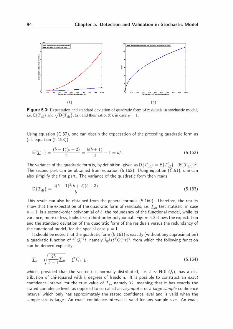
94 Chapter 5. Detection and Validation in Stochastic Model
0 100 200 300 400 500 600 700 800 900 10000
1
2
3
4
5
6x 10
5
Reduadancy of functional model (b)
Ex
pe
cta
tio
n &
Sta
nd
ard
de
via
tio
n
Expectation of quadratic formStd. dev. of quadratic form
(a)
0 100 200 300 400 500 600 700 800 900 10000
2
4
6
8
10
12
Reduadancy of functional model (b)
Ra
tio
Ratio of expectation and Std. dev. of quadratic form
(b)
Figure 5.3: Expectation and standard deviation of quadratic form of residuals in stochastic model,
i.e. E{T df} and√
D{T df}, (a), and their ratio, (b), in case p = 1.
Using equation (C.37), one can obtain the expectation of the preceding quadratic form as(cf. equation (5.153))
E{T df} =(b− 1)(b + 2)
2=
b(b + 1)
2− 1 = df . (5.162)
The variance of the quadratic form is, by definition, given as D{T df} = E{T 2df}−(E{T df})2.
The second part can be obtained from equation (5.162). Using equation (C.51), one canalso simplify the first part. The variance of the quadratic form then reads
D{T df} =2(b− 1)2(b + 2)(b + 3)
b. (5.163)
This result can also be obtained from the general formula (5.160). Therefore, the resultsshow that the expectation of the quadratic form of residuals, i.e. T df test statistic, in casep = 1, is a second-order polynomial of b, the redundancy of the functional model, while itsvariance, more or less, looks like a third-order polynomial. Figure 5.3 shows the expectationand the standard deviation of the quadratic form of the residuals versus the redundancy ofthe functional model, for the special case p = 1.
It should be noted that the quadratic form (5.161) is exactly (without any approximation)a quadratic function of tT Q−1
t t, namely b−12b
(tT Q−1t t)2, from which the following function
can be derived explicitly:
T b =
√
2b
b− 1T df = tT Q−1
t t , (5.164)
which, provided that the vector t is normally distributed, i.e. t ∼ N(0, Qt), has a dis-tribution of chi-squared with b degrees of freedom. It is possible to construct an exactconfidence interval for the true value of T b, namely Tb, meaning that it has exactly thestated confidence level, as opposed to so-called an asympotic or a large-sample confidenceinterval which only has approximately the stated confidence level and is valid when thesample size is large. An exact confidence interval is valid for any sample size. An exact
5.4 The overall model test 95
two-sided confidence interval (1− α) for Tb reads then
χ2b,1−α
2≤ Tb ≤ χ2
b, α2, (5.165)
with χ2b, α
2, the critical value obtained from the inverse of the chi-square cumulative dis-
tribution function. Substituting for Tb from equation (5.164) and solving for Tdf , i.e.transforming back from Tb into Tdf , gives a confidence interval for Tdf as follows:
b− 1
2bχ4
b,1−α2≤ Tdf ≤
b− 1
2bχ4
b, α2, (5.166)
with notation χ4b, α
2= (χ2
b, α2)2. In the case that b is sufficiently large, the chi-square
distribution may be approximated by a normal one, i.e. χ2(b, 0) ≈ N(b, 2b). In this case,the critical value reads χ2
b, α2≈ Xα
2with
Xα2
=√
2bZα2
+ b . (5.167)
Since the standard normal distribution is a symmetric one about zero, it follows Z1−α2
=−Zα
2. Substitution of the preceding terms in equation (5.166) gives an asymptotic confi-
dence interval for Tdf as
b2
2−√
2b32 Zα
2+ bZ2
α2≤ Tdf ≤
b2
2+√
2b32 Zα
2+ bZ2
α2. (5.168)
5.4.5 Approximation of quadratic form
What we want to mention here is the complexity of the distribution of the quadratic formT df . In this subsection an approximation for this quadratic form is derived, and a functionof it for which the distribution is completely known. To reach this goal, let us rewrite thequadratic form of the residuals for the stochastic model, i.e. equation (5.142) in terms oft vector, as follows:
T df = 12(tT Q−1
t t)2 − lT σ= 1
2(tT Q−1
t t)2 − liσi
= 12(tT Q−1
t t)2 − 12tT Q−1
t [σiQti ]Q−1t t
= 12(tT Q−1
t t)2 − 12tT Q−1
t QtQ−1t t .
(5.169)
Using the approximation Qt = Qt, one obtains
T df ≈1
2(tT Q−1
t t)2 − 1
2tT Q−1
t t = T ′df . (5.170)
This approximation is denoted as T ′df . Therefore, T df ≈ T ′
df . The distribution of thisapproximation is still complicated. It is not however difficult to show that the expectationand the dispersion of this approximated statistic read
E{T ′df} =
b(b + 1)
2= df + p ; D{T ′
df} = 2b3 + 8b2 + 8.5b , (5.171)
respectively. It is now possible to derive a function of this new statistic whose distributionis completely known. To follow this, equation (5.169) can be rewritten as
T df =1
2(tT Q−1
t t)2 − 1
2tT Q−1
t t− ǫ = T ′df − ǫ , (5.172)
96 Chapter 5. Detection and Validation in Stochastic Model
with
ǫ =1
2
(
tT Q−1t QtQ
−1t t− tT Q−1
t t)
. (5.173)
If we now define T b = tT Q−1t t it then follows that (see appendix B.5)
T ′b + ǫ′ ≈ 1
2
(√
8(T df + ǫ) + 1 + 1)
≈ T b = tT Q−1t t (5.174)
where the bias statistic ǫ′ is approximated as
ǫ′ ≈ 1
2
[
tT Q−1t QtQ
−1t t
tT Q−1t t
− 1
]
. (5.175)
Neglecting the bias terms ǫ and ǫ′ in equation (5.174) yields
T ′b ≈ T b =
1
2
(√
8T ′df + 1 + 1
)
= tT Q−1t t ∼ χ2(b, 0) (5.176)
Note that this approximation gets better and better when b, the redundancy of the func-tional model, becomes larger and larger (see example 5.8). In fact, the estimator T ′
b is aconsistent estimator of Tb. This is an interesting result as the preceding function (statistic)is the quadratic form of the residuals for the functional model, denoted as T b. Therefore,the statistic of the overall model test, both for the functional and the stochastic model,is identical. That is, the T b test statistic used in the functional model is a good generalindicator of the presence of some blunders (gross errors) in the observations. On the otherhand, with a large enough b, it can be interpreted as a general indication of detectingmisspecifications in the stochastic model as well.
An exact two-sided confidence interval (1 − α) for Tb (or accordingly an asymptoticconfidence interval for T ′
b) reads then
χ2b,1−α
2≤ T ′
b ≤ χ2b, α
2(5.177)
Substituting Tb and solving for T ′df , i.e. transforming back to the original function, from
Tb to T ′df , gives an approximate confidence interval for T ′
df (or an asymptotic approximateconfidence interval for Tdf) as follows:
1
2
(
χ4b,1−α
2− χ2
b,1−α2
)
≤ T ′df ≤
1
2
(
χ4b, α
2− χ2
b, α2
)
(5.178)
Again, if b is sufficiently large, the chi-square distribution can be approximated by a normalone for which the critical value reads χ2
b, α2≈√
2bZα2
+ b.
Example 5.8 Let us consider the simplest case with only one variance component in the sto-chastic model, namely p = 1. In this case, Qy = σ2Q, which gives
Qt = σ2BT Q1B, Qt = σ2BT Q1B . (5.179)
Substitution of the preceding terms into equation (5.175) yields
ǫ′ ≈ 1
2
[σ2
1
σ2− 1
]
. (5.180)
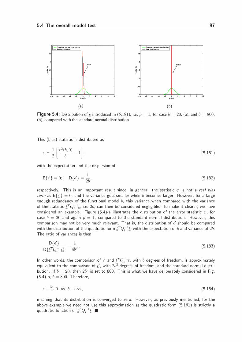
5.4 The overall model test 97
−10 −8 −6 −4 −2 0 2 4 6 8 100
0.5
1
1.5
2
2.5
3
x−axis
y−
ax
is
f(x
)Standard normal distributionReal distribution
b=20
(a)
−10 −8 −6 −4 −2 0 2 4 6 8 100
0.5
1
1.5
2
2.5
3
x−axis
y−
ax
is
f(x
)
Standard normal distributionReal distribution
b=800
(b)
Figure 5.4: Distribution of ǫ introduced in (5.181), i.e. p = 1, for case b = 20, (a), and b = 800,
(b), compared with the standard normal distribution
This (bias) statistic is distributed as
ǫ′ ≃ 1
2
[χ2(b, 0)
b− 1
]
, (5.181)
with the expectation and the dispersion of
E{ǫ′} = 0; D{ǫ′} =1
2b, (5.182)
respectively. This is an important result since, in general, the statistic ǫ′ is not a real biasterm as E{ǫ′} = 0, and the variance gets smaller when b becomes larger. However, for a largeenough redundancy of the functional model b, this variance when compared with the varianceof the statistic tT Q−1
t t, i.e. 2b, can then be considered negligible. To make it clearer, we haveconsidered an example. Figure (5.4)-a illustrates the distribution of the error statistic ǫ′, forcase b = 20 and again p = 1, compared to the standard normal distribution. However, thiscomparison may not be very much relevant. That is, the distribution of ǫ′ should be comparedwith the distribution of the quadratic form tT Q−1
t t, with the expectation of b and variance of 2b.The ratio of variances is then
D{ǫ′}D{tT Q−1
t t}=
1
4b2. (5.183)
In other words, the comparison of ǫ′ and tT Q−1t t, with b degrees of freedom, is approximately
equivalent to the comparison of ǫ′, with 2b2 degrees of freedom, and the standard normal distri-bution. If b = 20, then 2b2 is set to 800. This is what we have deliberately considered in Fig.(5.4)-b, b = 800. Therefore,
ǫ′ −→D 0 as b→∞ , (5.184)
meaning that its distribution is converged to zero. However, as previously mentioned, for theabove example we need not use this approximation as the quadratic form (5.161) is strictly aquadratic function of tT Q−1
t t. �
98 Chapter 5. Detection and Validation in Stochastic Model
5.5 Summary and concluding remarks
We generalized the idea of detection and validation into the stochastic model. It was aimedto find misspecifications in the stochastic model, to improve an existing covariance matrix,and to test the general validity of the stochastic model. This was done by introducingthe w-test, the v-test, and the overall model test with the stochastic model in systematicanalogy with testing in the functional model. We gave expressions for these test statisticsand derived the distributions for the w-test and the v-test statistic based on the normalityassumptions of the original observables y or t. For the examples given, when the redundancyb of the functional model is large enough, the distributions can be approximated by the(standard) normal distribution.
The overall model test statistic has in general a complicated form of distribution becauseof the complicated nature in which it depends on y or e. For some special cases, it mightbe possible to determine the exact distribution of equation (5.143). We considered anapproximation for this test statistic of which a function of this approximation has thewell-known chi-squared distribution. But, in general, one will have to rely on alternativecomputer-based techniques such as Monte-Carlo simulation or bootstrapping to make forinstance bootstrap confidence intervals. One may consider the simplest technique, thepercentile method. This method works well when the statistic used has a symmetricdistribution. The percentile method requires a large number of Monte Carlo replicationsfor the intervals to be both accurate (i.e. be as small as possible for the given confidencelevel) and nearly exact (i.e. if the procedure were repeated many times the percentage ofintervals that would actually include the ’true’ parameter value is approximately the statedconfidence level). For more information we refer to Efron and Tibshirani (1993)
Multivariate Variance-Covariance Analysis 66.1 Introduction
The primary purpose of this chapter is to introduce basic concepts of a multivariate statis-tical analysis which occurs frequently in practice. It may be helpful to think of the ‘analysis’as involving multiple dependent models. Experiments produce data where measurementswere obtained on one repeated model. In repeated model analysis, the multiple dependentvariables are the same measures (e.g. they are repeated over time). In multivariate models,the multiple dependent variables are measures of multiple outcomes, usually measured atthe same point in time. For example, a repeated model might be used to analyze the ver-tical components measured at three successive months while a multivariate analysis mightbe used to model three coordinate components (north, east, and vertical) at a single pointin time. The analysis of (co)variance is often applied in a multivariate model, if the effectsof factors can be explained by several characteristics. This is called a multivariate analysisof (co)variance. Multivariate models can also be set up if observations are repeated atdifferent times. In this case we can record temporal changes of a phenomenon.
A multivariate linear model, also known as a repeated linear model, is in fact an extensionof the univariate linear model. If for one design matrix in a Gauss-Markov model insteadof one observation vector several observation vectors with identical covariance matricesare given and the corresponding parameter vectors have to be determined, the model isreferred to as a multivariate Gauss-Markov model. We consider a generalization of theunivariate linear model E{y} = Ax, D{y} = σ2Q, when the variance σ2 of unit weightis unknown. This is in fact the simplest form of an unknown covariance matrix in a linearmodel. One can for instance show that the expressions for the BLUE of x, y, and e areinvariant against a change in the variance σ2 (see chapter 3). We will show in fact thatsuch an independence of the variance holds true also for a multivariate linear model.
In order to properly understand the estimation and validation of these model parameters,a foundation in multivariate statistics is needed. In particular, we may think of conceptssuch as variances and covariances (or correlations) between different groups (models). Weshow how the estimation and validation of (co)variance components can be expressed interms of the least-squares residuals. An advantage of the multivariate approach is to allowfor designs of experiments where the resulting parameter estimators will be uncorrelated,thus making it easier to interpret results. One might approach multivariate outcomes byexamining each outcome separately. There might be dangers with this, however. Withunivariate model analysis we may not use the whole observables in an optimal way. Oneproblem is that we are not doing multiple comparisons on the same data. More importantly,we usually expect the multiple outcomes to be correlated, and we may wish to determineif the outcomes are affected by treatment factors independent of other outcomes. We
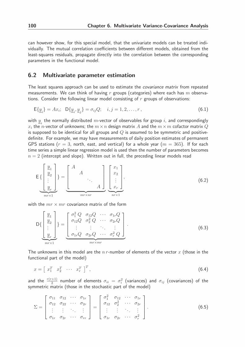
100 Chapter 6. Multivariate Variance-Covariance Analysis
can however show, for this special model, that the univariate models can be treated indi-vidually. The mutual correlation coefficients between different models, obtained from theleast-squares residuals, propagate directly into the correlation between the correspondingparameters in the functional model.
6.2 Multivariate parameter estimation
The least squares approach can be used to estimate the covariance matrix from repeatedmeasurements. We can think of having r groups (categories) where each has m observa-tions. Consider the following linear model consisting of r groups of observations:
E{yi} = Axi; D{y
i, y
j} = σijQ; i, j = 1, 2, . . . , r , (6.1)
with yithe normally distributed m-vector of observables for group i, and correspondingly
xi the n-vector of unknowns; the m×n design matrix A and the m×m cofactor matrix Qis supposed to be identical for all groups and Q is assumed to be symmetric and positive-definite. For example, we may have measurements of daily position estimates of permanentGPS stations (r = 3, north, east, and vertical) for a whole year (m = 365). If for eachtime series a simple linear regression model is used then the number of parameters becomesn = 2 (intercept and slope). Written out in full, the preceding linear models read
E {
y1
y2
...y
r
︸ ︷︷ ︸
mr×1
} =
AA
. . .
A
︸ ︷︷ ︸
mr×nr
x1
x2...xr
︸ ︷︷ ︸
nr×1
,(6.2)
with the mr ×mr covariance matrix of the form
D{
y1
y2
...y
r
︸ ︷︷ ︸
mr×1
} =
σ21 Q σ12Q · · · σ1rQ
σ12Q σ22 Q · · · σ2rQ
......
. . ....
σ1rQ σ2rQ · · · σ2r Q
︸ ︷︷ ︸
mr×mr
.(6.3)
The unknowns in this model are the n r-number of elements of the vector x (those in thefunctional part of the model)
x =[
xT1 xT
2 · · · xTr
]T, (6.4)
and the r(r+1)2
number of elements σii = σ2i (variances) and σij (covariances) of the
symmetric matrix (those in the stochastic part of the model)
Σ =
σ11 σ12 · · · σ1r
σ12 σ22 · · · σ2r...
.... . .
...σ1r σ2r · · · σrr
=
σ21 σ12 · · · σ1r
σ12 σ22 · · · σ2r
......
. . ....
σ1r σ2r · · · σ2r
. (6.5)
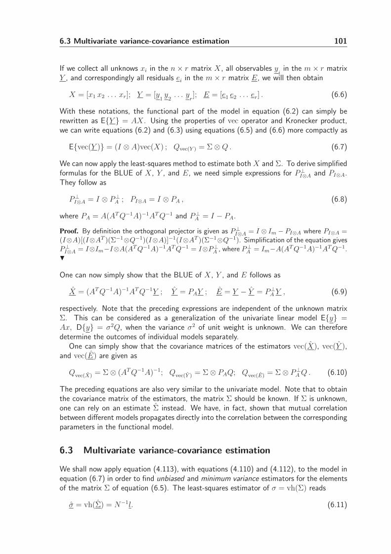
6.3 Multivariate variance-covariance estimation 101
If we collect all unknows xi in the n× r matrix X, all observables yiin the m× r matrix
Y , and correspondingly all residuals ei in the m× r matrix E, we will then obtain
X = [x1 x2 . . . xr]; Y = [y1y
2. . . y
r]; E = [e1 e2 . . . er] . (6.6)
With these notations, the functional part of the model in equation (6.2) can simply berewritten as E{Y } = AX. Using the properties of vec operator and Kronecker product,we can write equations (6.2) and (6.3) using equations (6.5) and (6.6) more compactly as
E{vec(Y )} = (I ⊗ A)vec(X) ; Qvec(Y ) = Σ⊗Q . (6.7)
We can now apply the least-squares method to estimate both X and Σ. To derive simplifiedformulas for the BLUE of X, Y , and E, we need simple expressions for P⊥
I⊗A and PI⊗A.They follow as
P⊥I⊗A = I ⊗ P⊥
A ; PI⊗A = I ⊗ PA , (6.8)
where PA = A(AT Q−1A)−1AT Q−1 and P⊥A = I − PA.
Proof. By definition the orthogonal projector is given as P⊥I⊗A = I ⊗ Im − PI⊗A where PI⊗A =
(I⊗A)[(I⊗AT )(Σ−1⊗Q−1)(I⊗A)]−1(I⊗AT )(Σ−1⊗Q−1). Simplification of the equation givesP⊥
I⊗A = I⊗Im−I⊗A(AT Q−1A)−1AT Q−1 = I⊗P⊥A , where P⊥
A = Im−A(AT Q−1A)−1AT Q−1.H
One can now simply show that the BLUE of X, Y , and E follows as
X = (AT Q−1A)−1AT Q−1Y ; Y = PAY ; E = Y − Y = P⊥A Y , (6.9)
respectively. Note that the preceding expressions are independent of the unknown matrixΣ. This can be considered as a generalization of the univariate linear model E{y} =Ax, D{y} = σ2Q, when the variance σ2 of unit weight is unknown. We can thereforedetermine the outcomes of individual models separately.
One can simply show that the covariance matrices of the estimators vec(X), vec(Y ),and vec(E) are given as
Qvec(X) = Σ⊗ (AT Q−1A)−1; Qvec(Y ) = Σ⊗ PAQ; Qvec(E) = Σ⊗ P⊥A Q . (6.10)
The preceding equations are also very similar to the univariate model. Note that to obtainthe covariance matrix of the estimators, the matrix Σ should be known. If Σ is unknown,one can rely on an estimate Σ instead. We have, in fact, shown that mutual correlationbetween different models propagates directly into the correlation between the correspondingparameters in the functional model.
6.3 Multivariate variance-covariance estimation
We shall now apply equation (4.113), with equations (4.110) and (4.112), to the model inequation (6.7) in order to find unbiased and minimum variance estimators for the elementsof the matrix Σ of equation (6.5). The least-squares estimator of σ = vh(Σ) reads
σ = vh(Σ) = N−1l. (6.11)
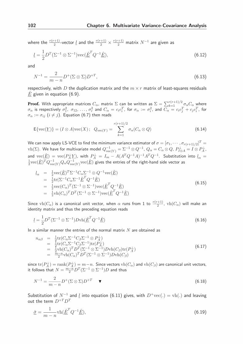
102 Chapter 6. Multivariate Variance-Covariance Analysis
where the r(r+1)2
-vector l and the r(r+1)2× r(r+1)
2matrix N−1 are given as
l =1
2DT (Σ−1 ⊗ Σ−1)vec(E
TQ−1E), (6.12)
and
N−1 =2
m− nD+(Σ⊗ Σ)D+T , (6.13)
respectively, with D the duplication matrix and the m× r matrix of least-squares residualsE given in equation (6.9).
Proof. With appropriate matrices Cα, matrix Σ can be written as Σ =∑r(r+1)/2
k=1 σαCα whereσα is respectively σ2
1, σ12, . . . , σ2r and Cα = cic
Ti , for σα := σ2
i , and Cα = cicTj + cjc
Ti , for
σα := σij (i 6= j). Equation (6.7) then reads
E{vec(Y )} = (I ⊗A)vec(X) ; Qvec(Y ) =
r(r+1)/2∑
k=1
σα(Cα ⊗Q) (6.14)
We can now apply LS-VCE to find the minimum variance estimator of σ = [σ1, · · · , σr(r+1)/2]T =
vh(Σ). We have for multivariate model Q−1vec(Y ) = Σ−1 ⊗Q−1, Qα = Cα ⊗Q, P⊥
I⊗A = I ⊗ P⊥A ,
and vec(E) = vec(P⊥A Y ), with P⊥
A = Im − A(AT Q−1A)−1AT Q−1. Substitution into lα =12vec(E)T Q−1
vec(Y )QαQ−1vec(Y )vec(E) gives the entries of the right-hand side vector as
lα = 12vec(E)T Σ−1CαΣ−1 ⊗Q−1vec(E)
= 12tr(Σ−1CαΣ−1E
TQ−1E)
= 12vec(Cα)T (Σ−1 ⊗ Σ−1)vec(E
TQ−1E)
= 12vh(Cα)T DT (Σ−1 ⊗ Σ−1)vec(E
TQ−1E)
(6.15)
Since vh(Cα) is a canonical unit vector, when α runs from 1 to r(r+1)2 , vh(Cα) will make an
identity matrix and thus the preceding equation reads
l =1
2DT (Σ−1 ⊗ Σ−1)Dvh(E
TQ−1E) (6.16)
In a similar manner the entries of the normal matrix N are obtained as
nαβ = 12tr(CαΣ−1CβΣ−1 ⊗ P⊥
A )= 1
2tr(CαΣ−1CβΣ−1)tr(P⊥A )
= 12vh(Cα)T DT (Σ−1 ⊗ Σ−1)Dvh(Cβ)tr(P⊥
A )= m−n
2 vh(Cα)T DT (Σ−1 ⊗ Σ−1)Dvh(Cβ)
(6.17)
since tr(P⊥A ) = rank(P⊥
A ) = m−n. Since vectors vh(Cα) and vh(Cβ) are canonical unit vectors,it follows that N = m−n
2 DT (Σ−1 ⊗ Σ−1)D and thus
N−1 =2
m− nD+(Σ⊗ Σ)D+T
H (6.18)
Substitution of N−1 and l into equation (6.11) gives, with D+vec(.) = vh(.) and leavingout the term D+T DT
σ =1
m− nvh(E
TQ−1E), (6.19)
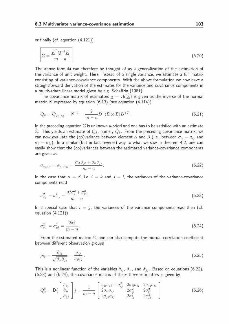
6.3 Multivariate variance-covariance estimation 103
or finally (cf. equation (4.121))
Σ =E
TQ−1E
m− n. (6.20)
The above formula can therefore be thought of as a generalization of the estimation ofthe variance of unit weight. Here, instead of a single variance, we estimate a full matrixconsisting of variance-covariance components. With the above formulation we now have astraightforward derivation of the estimates for the variance and covariance components ina multivariate linear model given by e.g. Schaffrin (1981).
The covariance matrix of estimators σ = vh(Σ) is given as the inverse of the normalmatrix N expressed by equation (6.13) (see equation (4.114))
Qσ = Qvh(Σ) = N−1 =2
m− nD+(Σ⊗ Σ)D+T . (6.21)
In the preceding equation Σ is unknown a-priori and one has to be satisfied with an estimateΣ. This yields an estimate of Qσ, namely Qσ. From the preceding covariance matrix, wecan now evaluate the (co)variance between element α and β (i.e. between σα = σij andσβ = σkl). In a similar (but in fact reverse) way to what we saw in theorem 4.2, one caneasily show that the (co)variances between the estimated variance-covariance componentsare given as
σσασβ= σσijσkl
=σikσjl + σilσjk
m− n. (6.22)
In the case that α = β, i.e. i = k and j = l, the variances of the variance-covariancecomponents read
σ2σα
= σ2σij
=σ2
i σ2j + σ2
ij
m− n. (6.23)
In a special case that i = j, the variances of the variance components read then (cf.equation (4.121))
σ2σα
= σ2σ2
i=
2σ4i
m− n. (6.24)
From the estimated matrix Σ, one can also compute the mutual correlation coefficientbetween different observation groups
ρij =σij
√σiiσjj
=σij
σiσj
. (6.25)
This is a nonlinear function of the variables σij, σii, and σjj. Based on equations (6.22),(6.23) and (6.24), the covariance matrix of these three estimators is given by
Qijσ = D{
σij
σii
σjj
} =1
m− n
σiiσjj + σ2ij 2σiiσij 2σjjσij
2σiiσij 2σ2ii 2σ2
ij
2σjjσij 2σ2ij 2σ2
jj
(6.26)
104 Chapter 6. Multivariate Variance-Covariance Analysis
To obtain the variance of the correlation coefficient ρij, one needs to apply the errorpropagation law to the linearized form of equation (6.25). The Jacobian (vector) of ρij isgiven as (take partial derivatives of equation (6.25) with respect to σij, σii, and σjj)
J = ρij
[1
σij
−1
2σii
−1
2σjj
]
(6.27)
Application of the error propagation law yields σ2ρij
= JQijσ JT . Substituting Qij
σ and J ,
respectively, from equations (6.26) and (6.27) yields
σ2ρij
=(1− ρij)
2
m− n(6.28)
If ρij = 0, it follows that σ2ρij
= 1m−n
.
6.4 Multivariate variance-covariance validation
6.4.1 The w-test statistic
Let us consider again the multivariate linear model given in equation (6.7). We are nowgoing to apply the idea of hypothesis testing to the stochastic part of this model. For thew-test statistic, the following null and alternative hypotheses are put forward:
Ho : D{vec(Y )} = σ20I ⊗Q versus Ha : D{vec(Y )} = (σ2
0I +∇Cα)⊗Q , (6.29)
where ∇ is an unknown parameter and Cα is an arbitrary r × r matrix. In this section wewill restrict ourselves to the case that σ2
0 is known. This means, under the null hypothesis,that all groups of observables have the same known variance component σ2
0 and that theobservable groups are uncorrelated. We want now to test this hypothesis using the w-teststatistic. For this purpose we can use the special case introduced in section 5.2.5 (seeequation (5.75)). We just need to substitute the terms from the multivariate model ase← vec(E), Qy ← σ2
0I ⊗Q, Cy ← Cα⊗Q, and P⊥A ← I ⊗P⊥
A . By doing so and after afew matrix operations, the following w-test statistic can be given:
w =
12σ4
0tr(CαE
TQ−1E)− b
2σ20tr(Cα)
[b
2σ40tr(CαCα)
]1/2. (6.30)
Under Ho, the preceding test statistic is distributed as w ∼∑k λkχ2k(1, 0)−m0, where m0
is the constant term on the right-hand side of equation (6.30) divided by the denominator,and the eigenvalues λk follow from
∣∣Cα ⊗ P⊥
A − λ[2b tr(CαCα)]1/2Irm
∣∣ = 0 . (6.31)
We will now consider two important cases which can frequently be used in practice. Theyare related to the testing of variances and covariances.
6.4 Multivariate variance-covariance validation 105
Testing of variances
In order to test whether or not the predefined variance components σ20 are appropriate, in
equation (6.29), one can take Cα = cicTi . Therefore, tr(Cα) = tr(CαCα) = 1. One can
simply show that the w-test statistic (6.30) simplifies to
wii =1√2b
(eT
i Q−1ei
σ20
− b
)
. (6.32)
In order to obtain the distribution of the preceding test statistic, we need to computeλk from equation (6.31). It goes without saying that the only non-zero eigenvalue ofCα = cic
Ti is one. Therefore, the b-number of non-zero eigenvalues of Cα ⊗ P⊥
A are one.The eigenvalues λk then read λ1 = λ2 = ... = λb = 1√
2b. Therefore, under the null
hypothesis, the w-test statistic is distributed as
wii ∼1√2b
(χ2(b, 0)− b
). (6.33)
Denoting eTi Q−1ei = b× σ2
i , the preceding equations yield
σ2i
σ20
∼ χ2(b, 0)
b. (6.34)
This is very similar to and in fact a generalization of the distribution of the famous varianceof unit weight (see example 5.1). Here we were concerned about the variance component ofonly one group of observables. We may also want to consider a few groups of observablestogether. For example one can define Cα = cic
Ti + cjc
Tj (if two groups are assumed to
have an identical variance component) or Cα = I (if we consider all groups together).
Note 6.1 In equation (6.29) we assumed that σ20 is known. It is still possible to perform
hypotheses testing even though the variance component σ2 is unknown. In this case equiv-alent expressions for equations (6.32) and (6.33) can be given as (employ equations (5.81)and (5.82))
wii =1
√
2br(r − 1)
(reT
i Q−1ei −∑r
k=1 eTk Q−1ek
σ2
)
; r ≥ 2, (6.35)
and
wii ∼1
√
2br(r − 1)
(
(r − 1)χ21(b, 0)− χ2
2(b(r − 1), 0))
, (6.36)
respectively. Note that the value of the test statistic (but not its distribution) dependson the unknown variance component σ2 for which an estimate can be used as σ2 =(∑r
k=1 eTk Q−1ek)/br. ⊡
Testing of covariances
We can also test whether or not additional covariance components are needed to be in-troduced in the stochastic model. For this purpose we may take Cα = cic
Tj + cjc
Ti to see
106 Chapter 6. Multivariate Variance-Covariance Analysis
if the covariance component between groups i and j is in fact zero. With this structurewe have tr(Cα) = 0 and tr(CαCα) = 2. One can show that the w-test statistic (6.30)simplifies to
wij =1√b
(
eTi Q−1ej
σ20
)
. (6.37)
In order to determine the distribution of the above test statistic, we need to compute λk
from equation (6.31). One can simply show that the two non-zero eigenvalues of Cα are±1. Therefore, only 2b-number of eigenvalues of Cα ⊗ P⊥
A are non zero. They follow asλ1 = λ2 = ... = λb = 1
2√
band λb+1 = λb+2 = ... = λ2b = −1
2√
b. The preceding w-test
statistic is then distributed as
wij ∼1
2√
b
(χ2
1(b, 0)− χ22(b, 0)
), (6.38)
where χ21(b, 0) and χ2
2(b, 0) are two independent chi-squared distributions with b degreesof freedom. Denoting eT
i Q−1ej = b× σij, the preceding equations yield
ρij
=σij
σ20
∼ 1
2b
(χ2
1(b, 0)− χ22(b, 0)
), (6.39)
with ρij
the correlation coefficient between groups i and j. There are standard procedures
for computing the distribution of quadratic forms in normal variables. The reader is referredto e.g. Imhof (1961). Based on the central limit theorem for independent and identicallydistributed data, when the redundancy b is large enough, one can approximate the chi-squared distribution by a normal one. Taking these approximations into account, thepreceding equation reads
ρij
=σij
σ20
≃ N(0, 1/b). (6.40)
Here we were only concerned about the covariance component between two groups ofobservables. We may also want to consider a few groups together. For example we candefine Cα = cic
Tj + cjc
Ti + cic
Tk + ckc
Ti (three groups).
6.4.2 The v-test statistic
The idea here is to test whether or not it is possible to reduce the number of covariancecomponents. To perform the (co)variance significance test (v-test), we can, for instance,test the following null hypotheses versus the alternative ones:
1. Ho : Qy = Σ⊗Q, σii = σ0ii versus Ha : Qy = Σ⊗Q,
2. Ho : Qy = Σ⊗Q, σij = σ0ij versus Ha : Qy = Σ⊗Q,
3. Ho : Qy = Σ⊗Q, σii = σkk versus Ha : Qy = Σ⊗Q,
4. Ho : Qy = Σ⊗Q, σij = σik versus Ha : Qy = Σ⊗Q,
5. Ho : Qy = Σ⊗Q, σij = σkl versus Ha : Qy = Σ⊗Q.
6.4 Multivariate variance-covariance validation 107
To do the testing we can make use of equations (5.133) and (5.134) for v-test statisticand the corresponding eigenvalues associated with its distribution, respectively. However,since the constant terms c0 and dT N−1d do not have any effect on testing results, we willignore them both in the test statistic and its distribution. Therefore, equation (5.133) cannow be reformulated as
v = dασα = eQ−1y [
1
2dαn−1
αβQβ]Q−1y e , (6.41)
which is distributed as v ∼ ∑k λkχ2k. The eigenvalues associated with this distribution
can be given by the following equation:∣∣[dαn−1
αβQβ]Q−1y P⊥
A − 2λI∣∣ = 0. (6.42)
Note that this new test statistic, in general, is no longer of mean zero and variance one.To obtain the v-test statistics for the multivariate linear model we just need to substitute
the preceding terms as follows: e ← vec(E), Qy ← Σ ⊗ Q, Qβ ← Cβ ⊗ Q, and P⊥A ←
I ⊗ P⊥A . In the following we will make use of the canonical unit vector for dα, e.g.
dα = vh(cicTi ) or dα = vh(cic
Tj + cjc
Ti ) if i 6= j. When we specify values for α or
correspondingly for i and j, the term dαn−1αβ simplifies to n−1
αβ where the only free index
is β (it is in fact the αth row of N−1). Note that β becomes a summation index whenmultiplied with Qβ. We will first evaluate the term dαn−1
α,βQβ. For this purpose we use thefixed index as α ≡ i, j and the summation index as β ≡ k, l. Therefore, one obtains
[dαn−1α,βQβ] = [n−1
ij,klQkl] = [n−1ij,klckc
Tl ]⊗Q =
1
b[(σikσjl + σilσjk)ckc
Tl ]⊗Q . (6.43)
Equation (6.42) can therefore be reformulated for the multivariate model as∣∣[(σikσjl + σilσjk)ckc
Tl ]Σ−1 ⊗ P⊥
A − 2bλIrm
∣∣ = 0 , (6.44)
in which the usth entry of the matrix [(σikσjl + σilσjk)ckcTl ], i.e. the element of the uth
row and sth column, is given as
[(σikσjl + σilσjk)ckcTl ] = σuiσjs + σujσis . (6.45)
When post-multiplied with Σ−1, it follows that
[(σikσjl + σilσjk)ckcTl ]Σ−1 = σuiσjsσ
−1sv + σujσisσ
−1sv = σuiδjv + σujδiv , (6.46)
which simplifies to
[(σikσjl + σilσjk)ckcTl ]Σ−1 =
σuj if v = i;σui if v = j;0 if v 6= i, j.
(6.47)
Therefore, the matrix [(σikσjl + σilσjk)ckcTl ]Σ−1 is a zero matrix except for two columns,
namely i and j, with entries of the jth and ith columns of Σ, respectively (the ith and jth
columns have been interchanged). The two non-zero eigenvalues of this matrix are givenby the eigenvalues of the following matrix:
Λ =
[σij σii
σjj σij
]
=
[σij σ2
i
σ2j σij
]
. (6.48)
108 Chapter 6. Multivariate Variance-Covariance Analysis
The eigenvalues of the preceding matrix can easily be computed as
λmax = σij + σiσj; λmin = σij − σiσj. (6.49)
Since the matrix P⊥A is a projector it also has b-number of non-zero eigenvalues i.e. λ′
1 =... = λ′
b = 1. Equation (6.44) has therefore 2b-number of non-zero eigenvalues. In thefollowing we will consider different testing hypotheses (different possibilities for i and j)for which we present test statistics and their corresponding distributions.
Testing of σii = σ0ii
We consider here the null hypothesis Ho : Qy = Σ ⊗ Q, σii = σ0ii versus the alternative
one Ha : Qy = Σ⊗Q. Under the null hypothesis it is assumed that the value of variancecomponent σii is to be equal to the known value σ0
ii. To see how the v-test statistic andits distribution of the above testing hypotheses look like, one can take dα = vh(cic
Ti ). It
goes without saying that the test statistic (6.41) can be written as
v = vh(cicTi )vh(Σ) = σii =
eTi Q−1ei
b. (6.50)
In order to determine the distribution of the aforementioned statistic, i.e. v = σii, we needto compute the eigenvalues λk from equation (6.44) as (note that here dα = vh(cic
Ti ))
∣∣[σikσilckc
Tl ]Σ−1 ⊗ P⊥
A − bλIrm
∣∣ = 0. (6.51)
In a similar way to equation (6.47), one can show that
[σikσilckcTl ]Σ−1 =
{σui if v = i;0 if v 6= i.
(6.52)
Therefore, the matrix [σikσilckcTl ]Σ−1 is a zero matrix except for its ith column with entries
of the ith column of Σ. The only non-zero eigenvalue of this matrix is σii. The matrixP⊥
A is a projector with non-zero eigenvalues λ′1 = ... = λ′
b = 1. With these in mind, thenon-zero eigenvalues λ of equation (6.51) are given as
λ1 = λ2 = .... = λb =σii
b. (6.53)
Under the null hypothesis, the distribution of the test statistic σii then reads
σii ∼σ0
ii
bχ2(b, 0)⇒ σii
σ0ii
∼ χ2(b, 0)
b. (6.54)
The above result can be thought of as being a generalization of the testing of the varianceof unit weight. This is an interesting result and very simple indeed as the χ2(b, 0) is awell-known central chi-squared distribution. Note that we have obtained the same resultsusing the w-test statistic (see equation (6.34)).
6.4 Multivariate variance-covariance validation 109
Testing of σij = σ0ij
We consider here the null hypothesis Ho : Qy = Σ ⊗ Q, σij = σ0ij versus the alternative
one Ha : Qy = Σ ⊗ Q. Under the null hypothesis the value of covariance component σij
is equal to the known value σ0ij. To see how the v-test statistic and its distribution of the
above testing hypotheses look like, one can take dα = vh(cicTj + cjc
Ti ). One can simply
show that the v-test statistic is written as follows:
v = σij =eT
i Q−1ej
b. (6.55)
In order to determine the distribution of the aforementioned statistic, we need to computethe eigenvalues of equation (6.44). We have, in fact, obtained these values as thosepresented in equation (6.49). When taking into account the projector P⊥
A , one obtains
λ1 = λ2 = .... = λb =σij + σiσj
2b; λb+1 = λb+2 = .... = λ2b =
σij − σiσj
2b. (6.56)
Under the null hypothesis, the test statistic σij is thus distributed as
σij ∼1
2b
[(σ0
ij + σiσj)χ21(b, 0) + (σ0
ij − σiσj)χ22(b, 0)
], (6.57)
where χ21(b, 0) and χ2
2(b, 0) are two independent chi-squared distributions with b degreesof freedom. If the redundancy b is large enough, we may approximate the chi-squareddistributions with normal ones. In this case the preceding distribution approximately yields
σij ≃ σiσjN
(
ρ0ij,
1 + ρ0ij
2
b
)
, (6.58)
or
ρij≃ N
(
ρ0ij,
1 + ρ0ij
2
b
)
, (6.59)
where ρ0ij =
σ0ij
σiσjand ρ
ij=
σij
σiσjare the correlation coefficients. If we now want to test
the significance of the correlation coefficient, i.e. under null hypothesis if ρ0ij = 0, it then
follows that
ρij≃ N(0, 1/b), (6.60)
which is identical to what we found in equation (6.40).
Testing of σii = σkk
The goal here is to test whether or not the variance component of group i is the same asthat of group k. In a similar way to what was done previously, one can define the vector das dα = vh(cic
Ti − ckc
Tk ). The test statistic simplifies to
v = σii − σkk =1
b[eT
i Q−1ei − eTk Q−1ek]. (6.61)
110 Chapter 6. Multivariate Variance-Covariance Analysis
The eigenvalues associated with the distribution, apart from those of P⊥A , i.e. b-number of
ones, of v can be obtained from∣∣∣∣
[σii −σik
σik −σkk
]
−[
λ 00 λ
]∣∣∣∣= 0, (6.62)
which gives
λmax =1
2
[
σii − σkk +√
(σii + σkk)2 − 4σ2ik
]
, (6.63)
and
λmin =1
2
[
σii − σkk −√
(σii + σkk)2 − 4σ2ik
]
, (6.64)
Under the null hypothesis we have σii = σkk. Therefore, the v-test statistic is distributedas (take into account the projector P⊥
A )
v ∼√
σ2ii − σ2
ik
b
[
χ21(b, 0) + χ2
2(b, 0)]
. (6.65)
If we approximate χ21(b, 0) and χ2
2(b, 0) by two independent normal distributions N1(b, 2b)and N2(b, 2b), we obtain
v ≃ N
(
0,4(σ2
ii − σ2ik)
b
)
. (6.66)
The maximum possible variance of the v-test statistic occurs when the covariance com-ponent between groups i and k is not significant, i.e. when σik = 0. If σii and σik areunknown a-priori, one can have recourse to estimates of those as σii = 1
2(σii + σkk) and
σik = σik, respectively.
Testing of σij = σik
Here we want to test whether or not the covariance component σij equals σik (i is thecommon index). To perform this test, one can define dα = vh(cic
Tj + cjc
Ti − cic
Tk − ckc
Ti )
from which it can be concluded that
v = σij − σik =1
b[eT
i Q−1ej − eTi Q−1ek]. (6.67)
The matrix Λ, a matrix whose eigenvalues are associated with the distribution of the v-teststatistic, is then given by
Λ =
σij − σik σii −σii
σjj − σjk σij −σij
σjk − σkk σik −σik
, (6.68)
in which the third column is a multiple of the second column. Therefore, the precedingmatrix is of rank 2. The eigenvalues of Λ then can be given as
λmax = σij − σik + σi
√
σjj + σkk − 2σjk, (6.69)
6.4 Multivariate variance-covariance validation 111
and
λmin = σij − σik − σi
√
σjj + σkk − 2σjk; λ3 = 0. (6.70)
Therefore, under the null hypothesis, the v-test statistic is distributed according to
v ∼ σi
√σjj + σkk − 2σjk
2b
[
χ21(b, 0)− χ2
2(b, 0)]
. (6.71)
which can be approximated by a normal distribution as
v ≃ N
(
0,σii(σjj + σkk − 2σjk)
b
)
. (6.72)
If the (co)variance components σii, σjj, σkk, and σjk are unknown a-priori, one can relyon the estimates σii, σjj, σkk, and σjk, respectively.
Testing of σij = σkl
The goal here is to see whether or not the covariance component σij equals σkl. To performthis test, one can define dα = vh(cic
Tj +cjc
Ti −ckc
Tl −clc
Tk ) from which it can be concluded
that
v = σij − σkl =1
b[eT
i Q−1ej − eTk Q−1el]. (6.73)
The matrix Λ, a matrix whose eigenvalues are associated with the distribution of thepreceding test statistic reads then
Λ =
σij σii −σil −σik
σjj σij −σjl −σjk
σjk σik −σkl −σkk
σjl σil −σll −σkl
, (6.74)
which, in general, is of rank 4. Denoting the eigenvalues of Λ as λ1, λ2, λ3 and λ4, thetest statistic v is distributed as
v ∼ 1
2b
[λ1χ
21(b, 0) + λ2χ
22(b, 0) + λ3χ
23(b, 0) + λ4χ
24(b, 0)
]. (6.75)
Under the null hypothesis and when σil = σjk = σjl = σik = 0 it follows that
λ1 = (σij + σiσj); λ2 = (σij − σiσj);λ3 = −(σij + σkσl); λ4 = −(σij − σkσl).
(6.76)
Again, if we approximate the chi-squared distributions with normal ones, equation (6.75)yields
v ≃ N
(
0,
∑4u=1 λ2
u
2b
)
. (6.77)
If in addition σi = σj = σk = σl, the preceding distribution reads
v ≃ N
(
0,2(σii + σij)
2
b
)
. (6.78)
112 Chapter 6. Multivariate Variance-Covariance Analysis
6.4.3 Overall model test
Let us now obtain the overall model test for the multivariate model. Under the nullhypothesis the stochastic model reads Qvec(Y ) = Σ ⊗ Q, in which we only consider thatΣ is known. Under the alternative hypothesis the covariance matrix is fully unknown (seee.g. equation (5.139)).
Σ = Σ0 known In multivariate model we need to obtain T df where df is defined as
df = rb(rb+1)2
. We can extend example 5.7 and equation (5.145) for a multivariate model.
We should substitute e← vec(E), Q−1y ← Σ−1 ⊗Q−1, and b← rb. One will then obtain
T df =1
2tr(Σ−1E
TQ−1E) tr(Σ−1E
TQ−1E)− tr(Σ−1E
TQ−1E) +
rb
2, (6.79)
which can have a complicated distribution. However, if we use the function T rb =√
2T df − rb + 1 + 1, it then follows that
T rb = tr(Σ−1ETQ−1E), (6.80)
which is distributed as T rb ∼ χ2(rb, 0).
GPS Geometry-Free Model 77.1 Introduction
The geometry-free observation model is one of the simplest approaches to integer GPSdouble differenced ambiguity estimation. This linear model dispenses with geometric apriori information and parameterizes the GPS observations simply in carrier-phase ambigu-ities and satellite-receiver ranges. Although simple, this parameterization does imply thatan adjustment according to the geometry-free observation model does not allow a directestimation of the baseline coordinates. It is therefore not the common mode of operationfor surveying applications.
Of the two basic GPS observation types, namely carrier-phase and pseudorange observa-tions, phase observations are greatly the more precise. Although more precise, carrier-phaseobservations are inherently biased by unknown integer numbers of carrier wavelengths whichare called carrier-phase ambiguities. Therefore, the favorable precision of the carrier-phaseobservations can only be fully exploited for relative positioning if the ambiguities are esti-mated and kept fixed at their integer values. In this case, the carrier-phase observationsare corrected on the basis of these estimates (see later on).
In spite of the fact that the geometry-free approach is less well suited for surveyingapplications, its use does offer some advantages (see next section). Foremost of theseadvantages is the ease with which the geometry-free observation model can be implementedin computer code. This ease stems from the linearity of the observation model and itsindependence of satellite orbit information. In addition, the geometry-free observationmodel is also very versatile, as it will allow the estimation of ambiguities even if observationsto only two satellites are available and even if both receivers are moving. Moreover,ambiguities estimated with the geometry-free model are also known to be free from residualtropospheric delay in the observations, as these delays are automatically lumped with thesatellite-receiver ranges. Therefore, for some applications, like data analysis and ionospheremonitoring, the geometry-free approach does have its appeal. Because of these advantages,the GPS geometry-free model will be used in this chapter as a favorable model for estimationof (co)variance components via the LS-VCE method. In the following section we considerthe geometry-free approach in more detail. We start with a description of the geometry-freeobservation model.
7.2 Functional and stochastic models
The geometry-free observation model consists of two parts: the functional model andthe stochastic model. The functional model relates the observations to the parameters ofinterest whereas the stochastic model describes the precision and the mutual correlation be-
114 Chapter 7. GPS Geometry-Free Model
tween the observations. The geometry-free functional model is based on the non-linearizeddouble differenced (DD) dual frequency pseudorange and carrier-phase observation equa-tions. Consider two receivers r and j simultaneously observing the same satellites s andk. Neglecting the dispersive DD ionospheric delay, the double differenced dual frequencypseudorange observation equations read (Jonkman, 1998)
psk
rj,L(ti) = ρsk
rj,L(ti) + eskrj,L(ti) , (7.1)
where (.)skrj is an abbreviation for (.)k
rj − (.)srj = (.)k
j − (.)kr − ((.)s
j − (.)sr), p denotes
the ’observed’ DD pseudoranges on the L1 or L2 frequency, e.g. C1 and P2, ρ denotesthe combination of all non-dispersive effects, L is either L1 or L2 frequency, e denotesthe pseudorange measurement errors on the L1 or L2 frequency, and ti indicates the timeinstant or epoch to which the observations refer. The most important difference betweenthe phase and the code observations is the entry of an integer DD carrier-phase ambiguityin the phase observation equations. Expressed in units of distance (m) rather then in cycles,the DD carrier-phase observation equations read
φsk
rj,L(ti) = ρsk
rj,L(ti) + λLaskrj,L + ǫsk
rj,L(ti) , (7.2)
where φ denotes the ’observed’ DD carrier-phase on the L1 or L2 frequency, a denotes theinteger carrier-phase ambiguities on the L1 or L2 frequency, and ǫ denotes the carrier-phasemeasurement errors on the L1 or L2 frequency. The dual frequency DD pseudorange andcarrier-phase observation equations can be summarized in the following linear system ofequations:
E{
pskrj,1
(ti)
pskrj,2
(ti)
φsk
rj,1(ti)
φsk
rj,2(ti)
} =
1 0 01 0 01 λ1 01 0 λ2
ρskrj (ti)
askrj,1
askrj,2
, (7.3)
where E denotes the expectation operator; the expectation of the measurement errors isassumed to be zero. This system of observation equations is referred to as the singleepoch geometry-free functional model. It refers to two receivers simultaneously observingtwo satellites. It is of course possible to include, in the functional model, the observationsto more than two satellites or even the observations of more than two receivers. In thisstudy, however, we will restrict ourselves to the observations of two receivers and to morethan two satellites. The above functional model over K epochs can be summarized in aconvenient vector-matrix notation as (still for two satellites)
E{
p1
p2
φ1
φ2
} =
I 0 0I 0 0I uλ1 0I 0 uλ2
ρa1
a2
(7.4)
with u = [1, 1, · · · , 1]T . If one, in one step, obtains a least squares solution of theabove, fixes the double differenced carrier-phase ambiguities to their integer values byusing the least-squares ambiguity decorrelation adjustment (LAMBDA) method (see Teu-nissen (1993, 1995); Verhagen (2005); Odijk (2002)) and ignores the stochastic behavior
7.2 Functional and stochastic models 115
of the integer valued ambiguities, one, in the next step, will be able to simplify the aboveobservation equations by subtracting from the observation vector a constant vector, namely[
0 0 λ1a1uT λ2a2u
T]T
, with a1 and a2 the least squares integer valued ambiguities.In this case, only the identity matrices of the design matrix will remain on the right handside of the preceding equation.
For a single observation epoch and dual frequency undifferenced pseudorange and carrier-phase observations, a very simple stochastic model reads
D{y} =
σ2p1
0 0 00 σ2
p20 0
0 0 σ2φ1
00 0 0 σ2
φ2
, (7.5)
where σ2pi
and σ2φi
, i = 1, 2 denote the variances of the undifferenced pseudorange andcarrier-phase observables. At this moment, mutual correlation between the observationsis assumed to be absent. Moreover, for the sake of simplicity, in some applications, theobservations on the L1 and L2 frequency are assumed to have a constant precision, i.e.σ2
p1= σ2
p2= σ2
p and σ2φ1
= σ2φ2
= σ2φ. This however may not be the case in general (see
next section); with these assumptions the stochastic model is very poor and immature.The purpose of this chapter is to come up with a realistic and adequate covariance matrixof GPS observables in case of a linear and simple geometry-free observation model. Weapply the least squares variance component estimation (LS-VCE) method to the stochasticpart of the geometry-free observation model. The construction of the covariance matrix(for undifferenced observables) starts from a scaled unit matrix per observation type andtakes place in different steps. In this application, the following six suppositions regardingthe noise of the undifferenced observables are considered:
1. to handle the ill-posedness of the VCE model (specifically for geometry-free model),the precision of the carrier-phase observables on L1 and L2 is assumed to be identical,
2. the precision of the pseudorange observations is assumed to be different for differentobservation types (on different frequencies),
3. the observables on the L1 and L2 frequency may or may not be correlated,
4. satellite elevation dependence of the observables precision will in part be considered,
5. time correlation of the observables is assumed to be absent (this may not be true forsome observation types for particular receivers), and
6. the correlation between different channels/satellites is assumed to be absent for allobservation types.
For detailed discussions on the noise characteristics of the GPS observables we refer toLangley (1997); Tiberius et al. (1999).
116 Chapter 7. GPS Geometry-Free Model
7.3 Sophisticated stochastic models
7.3.1 Satellite elevation dependence
If, in addition to the satellites s and k, we now assume that the receivers r and j are alsosimultaneously tracking the satellite l, the other DD pseudorange reads
psl
rj,L(ti) = ρsl
rj,L(ti) + eslrj,L(ti) , (7.6)
in which satellite s has been considered as reference. Assuming that the correlation betweenchannels is absent for each observation type, one can consider different precisions fordifferent channels. The covariance matrix of the undifferenced pseudorange observablesthen reads (two receivers)
Qy = diag(σ2ps
σ2ps
σ2pk
σ2pk
σ2pl
σ2pl) . (7.7)
Applying the error propagation law to the DD pseudoranges yields
QDy = JQyJ
T = 2
[σ2
ps+ σ2
pkσ2
ps
σ2ps
σ2ps
+ σ2pl
]
, (7.8)
where
J =
[1 −1 −1 1 0 01 −1 0 0 −1 1
]
. (7.9)
One can simplify the above covariance matrix if one assumes the same precision for differentchannels, i.e. σ2
ps= σ2
pk= σ2
pl= σ2
p. Therefore, if one neglects the satellite elevationdependence of GPS observation precision, one can estimate only one variance componentσ1 (a scale) for each observation type
QDy =
[4σ2
p 2σ2p
2σ2p 4σ2
p
]
σ1 , (7.10)
when the initial value of the pseudorange precision, σp = 30 cm, has been included in thecofactor matrix. In general, however, one needs to estimate 3 variance components foreach observation type
QDy =
[2σ2
p 2σ2p
2σ2p 2σ2
p
]
σs +
[2σ2
p 00 0
]
σk +
[0 00 2σ2
p
]
σl (7.11)
In other words, instead of estimating just one variance component, one can estimate differ-ent variance components for different satellites (or channels) observed at different elevationangles. The above structure can be employed for all observation types (e.g. for code andphase observations on L1 and L2).
7.3.2 Correlation between observation types
We now want to consider the correlation between different observation types. For the sakeof simplicity, one can ignore the satellite elevation dependence of the observables preci-sion. When dealing with four observation types, one needs to estimate 10 (co)variance
7.3 Sophisticated stochastic models 117
components, namely 4 variances and 6 covariances. As an example, consider the follow-ing covariance matrix for two types of undifferenced observations (e.g. single frequency),namely pseudorange and carrier phase (as before, 2 receivers simultaneously tracking 3satellites)
Qy =
[σ2
p I6 σpφI6
σpφI6 σ2φ I6
]
. (7.12)
From the above 12 observations one can create 4 DD equations; 2 DD pseudorange and 2DD carrier-phase observation equations. Applying the error propagation law, will give riseto the following covariance matrix for DD observations:
QDy =
[J 00 J
] [σ2
p I6 σpφI6
σpφI6 σ2φ I6
] [JT 00 JT
]
=
[σ2
p Q σpφQσpφQ σ2
φ Q
]
, (7.13)
where
Q = J JT =
[4 22 4
]
. (7.14)
When we have more satellites, namely k, Q can be generalized as well; qii = 4, qij =2, i 6= j and i, j = 1, 2, . . . , k − 1. Therefore, in general, the following covariance matrixshould be estimated by the LS-VCE method (dual frequency):
QDy =
σ2p1
Q σp1p2Q σp1φ1Q σp1φ2Qσp1p2Q σ2
p2Q σp2φ1Q σp2φ2Q
σp1φ1Q σp2φ1Q σ2φ1
Q σφ1φ2Qσp1φ2Q σp2φ2Q σφ1φ2Q σ2
φ2Q
, (7.15)
or
QDy =
σ2p1
σp1p2 σp1φ1 σp1φ2
σp1p2 σ2p2
σp2φ1 σp2φ2
σp1φ1 σp2φ1 σ2φ1
σφ1φ2
σp1φ2 σp2φ2 σφ1φ2 σ2φ2
⊗Q = Σ⊗Q , (7.16)
where ⊗ denotes the Kronecker product of two matrices. In our investigations, the initialvalues (undifferenced) σφi
= 0.003 m and σpi= 0.3 m, i = 1, 2 have also been included in
Q matrices. In other words, the Q matrices above have the same structure but, in general,different scales. Therefore, the above equation is just symbolically correct.
With four observation types, one needs to estimate 10 (co)variance components, namely4 variances and 6 covariances. Strictly speaking not all unknown components are estimable.The maximum number of estimable parameters is 6, e.g. 4 variances and 2 covariances orjust 6 covariances, etc (see example 4.10). The other problem as to the estimability is dueto the fact that two observation types are much more precise than the others, namely carrierphase when compared to the pseudoranges. This will cause the problem to be ill-posed forthe geometry-free model. That is, the estimated components of the precise observationsare highly correlated and poorly estimable. To handle the problem, one can assume thesame variance for both carrier-phase observations on L1 and L2. It should be noted, whendealing with 4 observation types as with GPS, only 3 components are precisely estimable,
118 Chapter 7. GPS Geometry-Free Model
namely one (co)variance component for carrier-phase observations and two (co)variancecomponents for pseudorange observations. When we deal with 5 observation types, e.g.φ1, φ2, C1, P1, and P2, 7 components are precisely estimable, namely 1 (co)variancecomponent for carrier-phase observations and all 6 (co)variance components of the codeobservations.
7.3.3 Time correlation of observables
We concentrate here on the off-diagonal elements (covariances) in the K m × K m co-variance matrix of one GPS observation type over K epochs, i.e. the covariance betweenepochs or time correlation, instead of between observation types. For the reason of con-venience, assume only two epochs of observations for one observation type (as before,2 receivers simultaneously tracking 3 satellites). The covariance matrix of undifferencedobservables then reads
Qy =
[σ2
(1) I6 σ(12)I6
σ(12)I6 σ2(2) I6
]
, (7.17)
in which σ2(1) and σ2
(2) are the variance components of the first and second epoch, respec-tively and σ(12) is the covariance between the two epochs. Applying the error propagationlaw will bring about the following covariance matrix for DD observations:
QDy =
[J 00 J
] [σ2
(1) I6 σ(12)I6
σ(12)I6 σ2(2) I6
] [JT 00 JT
]
=
[σ2
(1) Q σ(12)Q
σ(12)Q σ2(2) Q
]
, (7.18)
where again
Q = J JT =
[4 22 4
]
. (7.19)
If we have k satellites, Q can be generalized as qii = 4, qij = 2, i 6= j and i, j =1, 2, . . . , k−1. Therefore, in general, for K epochs, the following covariance matrix shouldbe estimated by the LS-VCE method:
QDy =
σ2(1) Q σ(12)Q · · · σ(1K)Q
σ(12)Q σ2(2) Q · · · σ(2K)Q
......
. . ....
σ(1K)Q σ(2K)Q · · · σ2(K) Q
, (7.20)
or
QDy =
σ2(1) σ(12) · · · σ(1K)
σ(12) σ2(2) · · · σ(2K)
......
. . ....
σ(1K) σ(2K) · · · σ2(K)
⊗Q . (7.21)
The above structure can be employed for all different observation types. The preced-ing covariance matrix contains K(K + 1)/2 (co)variance components, K variances and
7.4 Multivariate linear model 119
K(K − 1)/2 covariances. Since the observations are usually equidistant in time, assum-ing stationarity of the GPS observations implies that the elements on the negative-slopingdiagonals of the above equation should be equal (a symmetric Toeplitz matrix). In thiscase the (co)variance component σ(ij) is a function of the time difference τ = |j − i|,namely σ(ij) = στ = σ|j−i|. Therefore, the number of auto-(co)variance components willget reduced to K. The reader is referred to Tiberius and Kenselaar (2003).
7.4 Multivariate linear model
The LS-VCE model is a powerful method for the estimation of the stochastic model para-meters. However, the computational burden of this method is still a challenging problem.The procedure proposed in this section aims to reduce the computational load and memoryusage. For the GPS geometry-free model one can estimate the (co)variance componentsby using only a few epochs of observations. However, to improve the precision of the es-timates one usually likes using all available observations. Because of the special structureof the covariance matrix of observations and the design matrix, the final estimates can beeasily obtained. To this end, consider the following model of observation equations withunknown (co)variance components:
E{y} = Ax, Q =
p∑
k=1
σkQk (7.22)
with y the m × 1 vector of observables, A the m × n design matrix, x the n × 1 vectorof unknowns, Q the m × m covariance matrix of observables, Qk the m × m cofactormatrices, and σk the unknown (co)variance components to be estimated. Now this modelis repeated r times α = 1, . . . , r, where the unknown parameters are allowed to varybetween the groups. Moreover, the measurements of different groups are assumed to beuncorrelated. This model can, for example, be applied to the geometry-free observationmodel when first the observations are split into r groups or categories, second the timecorrelation of observables is absent, and third the statistical behavior of the integer DDcarrier-phase ambiguities is ignored and they are kept fixed. Such a multivariate model(repeated model) is of the form
E{
y(1)
y(2)
...y(r)
} =
A 0 · · · 00 A · · · 0...
.... . .
...0 0 · · · A
x(1)
x(2)
...x(r)
, Qy =
Q 0 · · · 00 Q · · · 0...
.... . .
...0 0 · · · Q
(7.23)
with y(i) and x(i) the observable vector and the unknown vector of group i, respectively.The same design matrix A appears for each group, but the unknowns in x are allowed tovary from group to group. One can prove that the final estimates are obtained by averagingthe groupwise estimates
σ =1
r
r∑
i=1
σ(i), or σk =1
r
r∑
i=1
σ(i)k , k = 1, . . . , p (7.24)
with the covariance matrix
Qσ =1
rN−1 (7.25)
120 Chapter 7. GPS Geometry-Free Model
where N is the normal matrix of a single group. Note that if certain (co)variance com-ponents can not be estimated in a single model (which is sometimes the case for thegeometry-free model), they can never be estimated if the model is repeated r times.
When a model repeats every 1 sec, collecting 10 (10 is arbitrary) secs of these datain one group (a 10-epoch group) is repeated every 10 secs. For the multivariate modelintroduced above, we now assume that the covariance matrix Q is the same for all 10-epochgroups as in equation (7.23). This is our strategy for handling a full hour of GPS data.
7.5 Presentation and interpretation of results
The estimates obtained should be presented as clearly as possible. For this purpose, usuallyvisualizing techniques are very appealing. Apart from that, when dealing with numbers,it is more convenient to demonstrate the numerical estimates in such a way that theyare readily understandable. For example, if our original observations are expressed in unitof meter (m), then the (co)variance components estimated by LS-VCE will be expressedin unit of m2 and the variance of these estimators in m4. It may not be convenient todeal with m2 and m4. In this section it is intended to derive simple formulas for standarddeviation estimators and correlation coefficients as well as their precision only for the reasonof presentation. Let σ2
i = σii and σσ2i
= σσiibe the variance estimator and its standard
deviation, respectively. They are both expressed in units of m2. To extract the moreconvenient indicators, let us apply the square root to the variance estimator which givesthe standard deviation estimator expressed in units of meters. To obtain the precision ofthis estimator, consider the following equation:
σi =√
σ2i =
√
σii. (7.26)
It is now possible to derive the precision of the variable σi, namely σσi, using the error
propagation law for non-linear functions. One can simply show that the precision of thestandard deviation estimate can be approximated using the following equation:
σσi≈
σσ2i
2σi
=σσii
2σi
(7.27)
where both σi and σσiiare given.
For correlation coefficients, assume that we are given the covariance estimate σij (m2)and its precision σσij
(m2) and two variance estimates σii (m2) and σjj (m2) with theirprecision σσii
(m2) and σσjj(m2). In addition to the standard deviations of the estimates,
there are also covariances between estimates. The 3×3 matrix Qijσ denotes the covariance
matrix of the estimates. In practice, it is more convenient to present the correlationcoefficient instead of the covariance estimate
ρ =σij
σi σj
=σij√
σii
√σjj
(7.28)
To obtain the variance of the correlation coefficient ρij, one needs to apply the errorpropagation law to the linearized form of the preceding equation which yields σ2
ρ = JQijσ JT ,
where J is the Jacobian vector given in equation (6.27). If we assume that the (co)variance
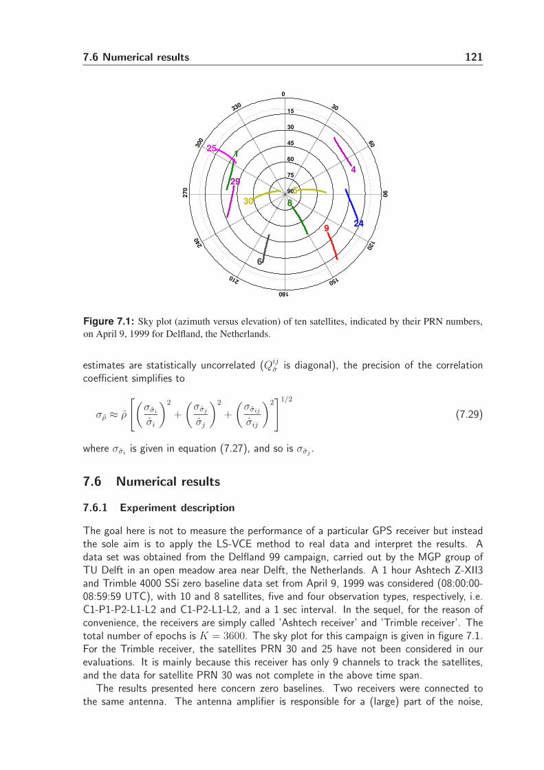
7.6 Numerical results 121
−50 0 50
−80
−60
−40
−20
0
20
40
60
80
0
30
60
90
120
150
180
210
240
270
300
33015
30
45
60
75
90
1
4
5
6
8
924
25
29
30
Figure 7.1: Sky plot (azimuth versus elevation) of ten satellites, indicated by their PRN numbers,
on April 9, 1999 for Delfland, the Netherlands.
estimates are statistically uncorrelated (Qijσ is diagonal), the precision of the correlation
coefficient simplifies to
σρ ≈ ρ
[(σσi
σi
)2
+
(σσj
σj
)2
+
(σσij
σij
)2]1/2
(7.29)
where σσiis given in equation (7.27), and so is σσj
.
7.6 Numerical results
7.6.1 Experiment description
The goal here is not to measure the performance of a particular GPS receiver but insteadthe sole aim is to apply the LS-VCE method to real data and interpret the results. Adata set was obtained from the Delfland 99 campaign, carried out by the MGP group ofTU Delft in an open meadow area near Delft, the Netherlands. A 1 hour Ashtech Z-XII3and Trimble 4000 SSi zero baseline data set from April 9, 1999 was considered (08:00:00-08:59:59 UTC), with 10 and 8 satellites, five and four observation types, respectively, i.e.C1-P1-P2-L1-L2 and C1-P2-L1-L2, and a 1 sec interval. In the sequel, for the reason ofconvenience, the receivers are simply called ’Ashtech receiver’ and ’Trimble receiver’. Thetotal number of epochs is K = 3600. The sky plot for this campaign is given in figure 7.1.For the Trimble receiver, the satellites PRN 30 and 25 have not been considered in ourevaluations. It is mainly because this receiver has only 9 channels to track the satellites,and the data for satellite PRN 30 was not complete in the above time span.
The results presented here concern zero baselines. Two receivers were connected tothe same antenna. The antenna amplifier is responsible for a (large) part of the noise,
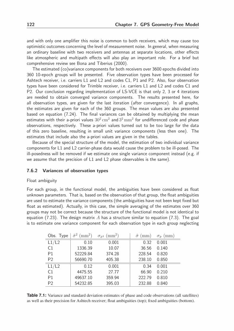
122 Chapter 7. GPS Geometry-Free Model
and with only one amplifier this noise is common to both receivers, which may cause toooptimistic outcomes concerning the level of measurement noise. In general, when measuringan ordinary baseline with two receivers and antennas at separate locations, other effectslike atmospheric and multipath effects will also play an important role. For a brief butcomprehensive review see Bona and Tiberius (2000).
The estimated (co)variance components for both receivers over 3600 epochs divided into360 10-epoch groups will be presented. Five observation types have been processed forAshtech receiver, i.e. carriers L1 and L2 and codes C1, P1 and P2. Also, four observationtypes have been considered for Trimble receiver, i.e. carriers L1 and L2 and codes C1 andP2. Our conclusion regarding implementation of LS-VCE is that only 2, 3 or 4 iterationsare needed to obtain converged variance components. The results presented here, forall observation types, are given for the last iteration (after convergence). In all graphs,the estimates are given for each of the 360 groups. The mean values are also presentedbased on equation (7.24). The final variances can be obtained by multiplying the meanestimates with their a-priori values 302 cm2 and 32 mm2 for undifferenced code and phaseobservations, respectively. These a-priori values turned out to be too large for the dataof this zero baseline, resulting in small unit variance components (less then one). Theestimates that include also the a-priori values are given in the tables.
Because of the special structure of the model, the estimation of two individual variancecomponents for L1 and L2 carrier-phase data would cause the problem to be ill-posed. Theill-posedness will be removed if we estimate one single variance component instead (e.g. ifwe assume that the precision of L1 and L2 phase observables is the same).
7.6.2 Variances of observation types
Float ambiguity
For each group, in the functional model, the ambiguities have been considered as floatunknown parameters. That is, based on the observation of that group, the float ambiguitiesare used to estimate the variance components (the ambiguities have not been kept fixed butfloat as estimated). Actually, in this case, the simple averaging of the estimates over 360groups may not be correct because the structure of the functional model is not identical toequation (7.23). The design matrix A has a structure similar to equation (7.3). The goalis to estimate one variance component for each observation type in each group neglecting
Obs. Type σ2 (mm2) σσ2 (mm2) σ (mm) σσ (mm)
L1/L2 0.10 0.001 0.32 0.001C1 1336.39 10.07 36.56 0.140P1 52229.84 374.28 228.54 0.820P2 56690.70 405.38 238.10 0.850
L1/L2 0.12 0.001 0.34 0.001C1 4475.55 27.77 66.90 0.210P1 49637.10 359.94 222.79 0.810P2 54232.85 395.03 232.88 0.840
Table 7.1: Variance and standard deviation estimates of phase and code observations (all satellites)
as well as their precision for Ashtech receiver; float ambiguities (top); fixed ambiguities (bottom).
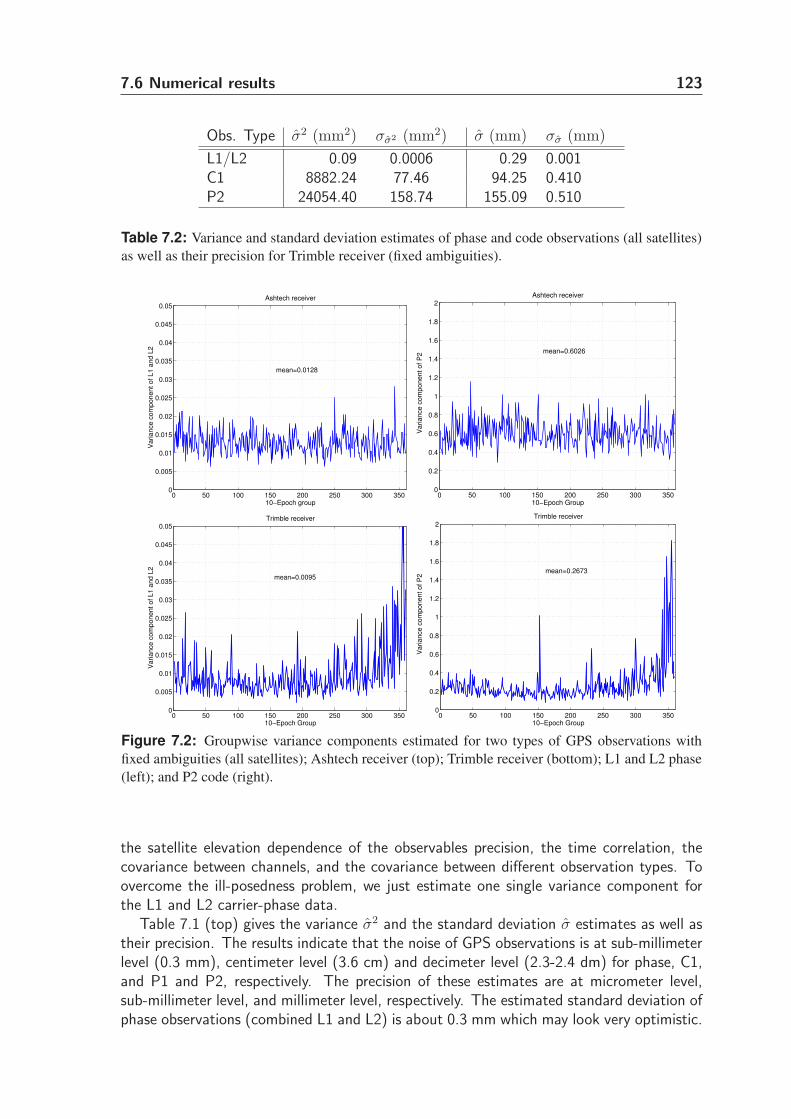
7.6 Numerical results 123
Obs. Type σ2 (mm2) σσ2 (mm2) σ (mm) σσ (mm)
L1/L2 0.09 0.0006 0.29 0.001C1 8882.24 77.46 94.25 0.410P2 24054.40 158.74 155.09 0.510
Table 7.2: Variance and standard deviation estimates of phase and code observations (all satellites)
as well as their precision for Trimble receiver (fixed ambiguities).
0 50 100 150 200 250 300 3500
0.005
0.01
0.015
0.02
0.025
0.03
0.035
0.04
0.045
0.05Ashtech receiver
10−Epoch group
Variance c
om
ponent of L1 a
nd L
2
mean=0.0128
0 50 100 150 200 250 300 3500
0.2
0.4
0.6
0.8
1
1.2
1.4
1.6
1.8
2Ashtech receiver
10−Epoch Group
Variance c
om
ponent of P
2 mean=0.6026
0 50 100 150 200 250 300 3500
0.005
0.01
0.015
0.02
0.025
0.03
0.035
0.04
0.045
0.05Trimble receiver
10−Epoch Group
Variance c
om
ponent of L1 a
nd L
2
mean=0.0095
0 50 100 150 200 250 300 3500
0.2
0.4
0.6
0.8
1
1.2
1.4
1.6
1.8
2Trimble receiver
10−Epoch Group
Va
ria
nce
co
mp
on
en
t o
f P
2
mean=0.2673
Figure 7.2: Groupwise variance components estimated for two types of GPS observations with
fixed ambiguities (all satellites); Ashtech receiver (top); Trimble receiver (bottom); L1 and L2 phase
(left); and P2 code (right).
the satellite elevation dependence of the observables precision, the time correlation, thecovariance between channels, and the covariance between different observation types. Toovercome the ill-posedness problem, we just estimate one single variance component forthe L1 and L2 carrier-phase data.
Table 7.1 (top) gives the variance σ2 and the standard deviation σ estimates as well astheir precision. The results indicate that the noise of GPS observations is at sub-millimeterlevel (0.3 mm), centimeter level (3.6 cm) and decimeter level (2.3-2.4 dm) for phase, C1,and P1 and P2, respectively. The precision of these estimates are at micrometer level,sub-millimeter level, and millimeter level, respectively. The estimated standard deviation ofphase observations (combined L1 and L2) is about 0.3 mm which may look very optimistic.
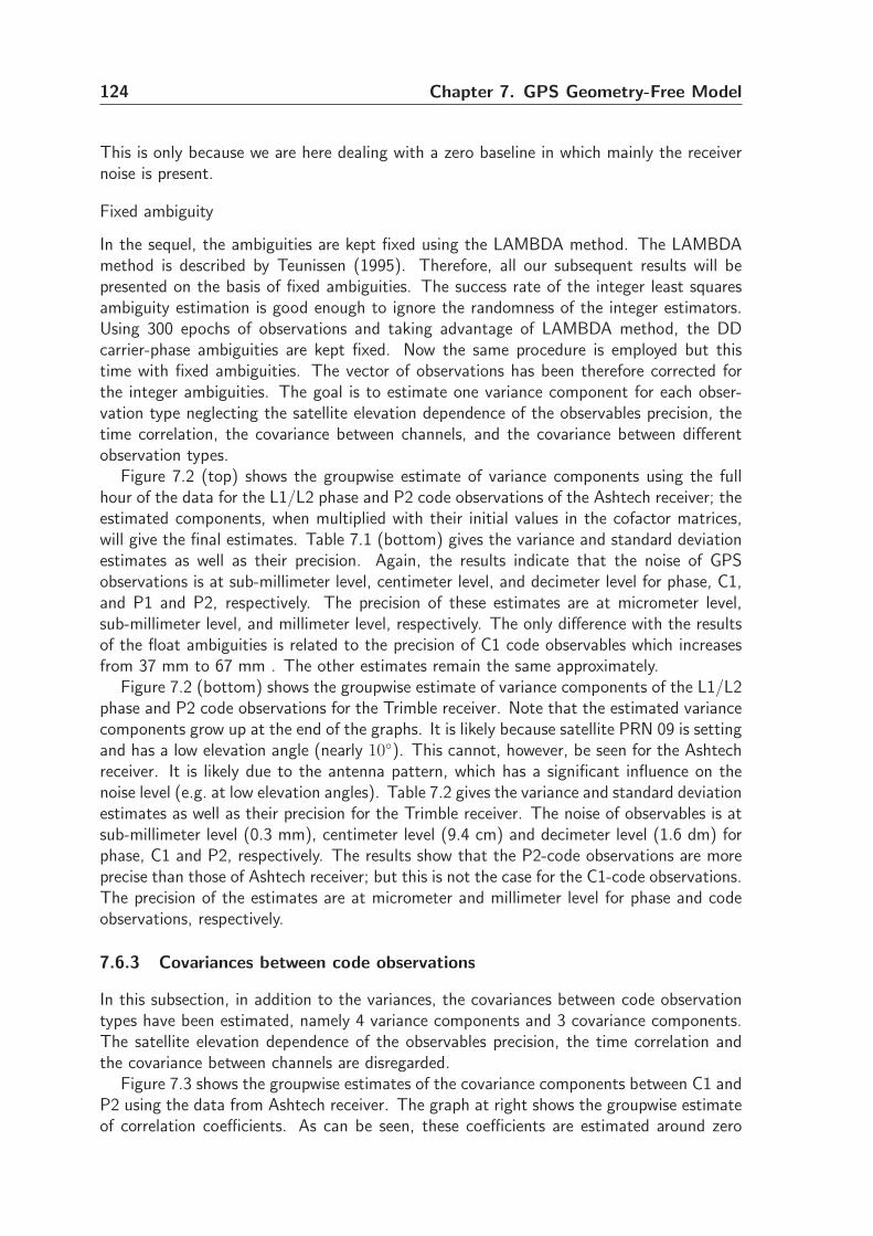
124 Chapter 7. GPS Geometry-Free Model
This is only because we are here dealing with a zero baseline in which mainly the receivernoise is present.
Fixed ambiguity
In the sequel, the ambiguities are kept fixed using the LAMBDA method. The LAMBDAmethod is described by Teunissen (1995). Therefore, all our subsequent results will bepresented on the basis of fixed ambiguities. The success rate of the integer least squaresambiguity estimation is good enough to ignore the randomness of the integer estimators.Using 300 epochs of observations and taking advantage of LAMBDA method, the DDcarrier-phase ambiguities are kept fixed. Now the same procedure is employed but thistime with fixed ambiguities. The vector of observations has been therefore corrected forthe integer ambiguities. The goal is to estimate one variance component for each obser-vation type neglecting the satellite elevation dependence of the observables precision, thetime correlation, the covariance between channels, and the covariance between differentobservation types.
Figure 7.2 (top) shows the groupwise estimate of variance components using the fullhour of the data for the L1/L2 phase and P2 code observations of the Ashtech receiver; theestimated components, when multiplied with their initial values in the cofactor matrices,will give the final estimates. Table 7.1 (bottom) gives the variance and standard deviationestimates as well as their precision. Again, the results indicate that the noise of GPSobservations is at sub-millimeter level, centimeter level, and decimeter level for phase, C1,and P1 and P2, respectively. The precision of these estimates are at micrometer level,sub-millimeter level, and millimeter level, respectively. The only difference with the resultsof the float ambiguities is related to the precision of C1 code observables which increasesfrom 37 mm to 67 mm . The other estimates remain the same approximately.
Figure 7.2 (bottom) shows the groupwise estimate of variance components of the L1/L2phase and P2 code observations for the Trimble receiver. Note that the estimated variancecomponents grow up at the end of the graphs. It is likely because satellite PRN 09 is settingand has a low elevation angle (nearly 10◦). This cannot, however, be seen for the Ashtechreceiver. It is likely due to the antenna pattern, which has a significant influence on thenoise level (e.g. at low elevation angles). Table 7.2 gives the variance and standard deviationestimates as well as their precision for the Trimble receiver. The noise of observables is atsub-millimeter level (0.3 mm), centimeter level (9.4 cm) and decimeter level (1.6 dm) forphase, C1 and P2, respectively. The results show that the P2-code observations are moreprecise than those of Ashtech receiver; but this is not the case for the C1-code observations.The precision of the estimates are at micrometer and millimeter level for phase and codeobservations, respectively.
7.6.3 Covariances between code observations
In this subsection, in addition to the variances, the covariances between code observationtypes have been estimated, namely 4 variance components and 3 covariance components.The satellite elevation dependence of the observables precision, the time correlation andthe covariance between channels are disregarded.
Figure 7.3 shows the groupwise estimates of the covariance components between C1 andP2 using the data from Ashtech receiver. The graph at right shows the groupwise estimateof correlation coefficients. As can be seen, these coefficients are estimated around zero
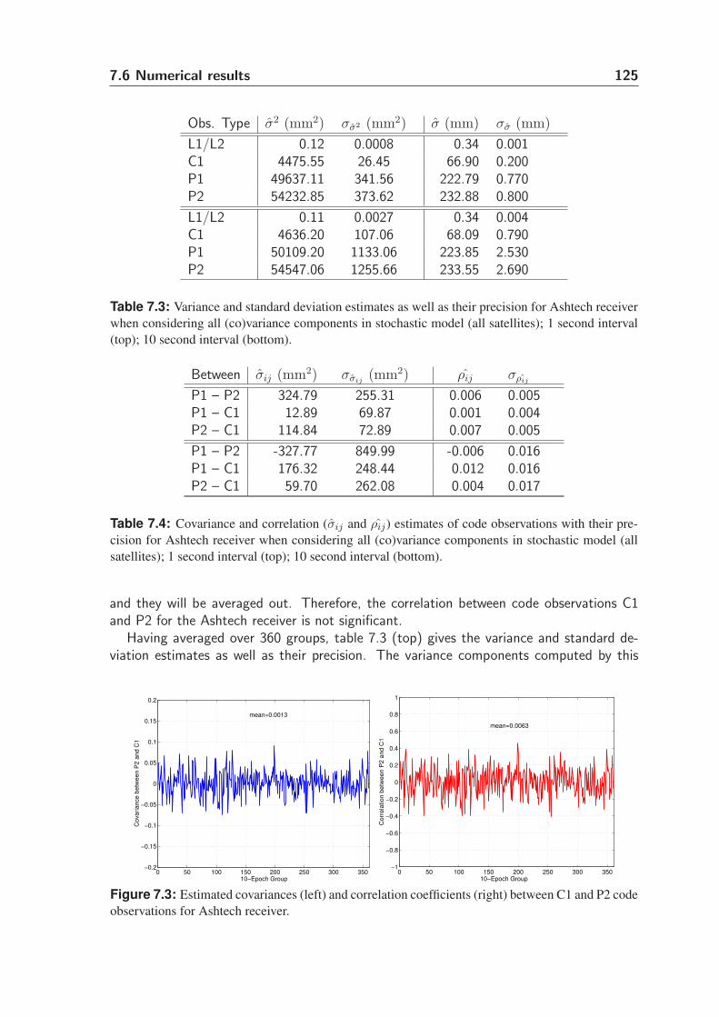
7.6 Numerical results 125
Obs. Type σ2 (mm2) σσ2 (mm2) σ (mm) σσ (mm)
L1/L2 0.12 0.0008 0.34 0.001C1 4475.55 26.45 66.90 0.200P1 49637.11 341.56 222.79 0.770P2 54232.85 373.62 232.88 0.800
L1/L2 0.11 0.0027 0.34 0.004C1 4636.20 107.06 68.09 0.790P1 50109.20 1133.06 223.85 2.530P2 54547.06 1255.66 233.55 2.690
Table 7.3: Variance and standard deviation estimates as well as their precision for Ashtech receiver
when considering all (co)variance components in stochastic model (all satellites); 1 second interval
(top); 10 second interval (bottom).
Between σij (mm2) σσij(mm2) ρij σρij
P1 – P2 324.79 255.31 0.006 0.005P1 – C1 12.89 69.87 0.001 0.004P2 – C1 114.84 72.89 0.007 0.005
P1 – P2 -327.77 849.99 -0.006 0.016P1 – C1 176.32 248.44 0.012 0.016P2 – C1 59.70 262.08 0.004 0.017
Table 7.4: Covariance and correlation (σij and ρij) estimates of code observations with their pre-
cision for Ashtech receiver when considering all (co)variance components in stochastic model (all
satellites); 1 second interval (top); 10 second interval (bottom).
and they will be averaged out. Therefore, the correlation between code observations C1and P2 for the Ashtech receiver is not significant.
Having averaged over 360 groups, table 7.3 (top) gives the variance and standard de-viation estimates as well as their precision. The variance components computed by this
0 50 100 150 200 250 300 350−0.2
−0.15
−0.1
−0.05
0
0.05
0.1
0.15
0.2
10−Epoch Group
Covariance b
etw
een P
2 a
nd C
1
mean=0.0013
0 50 100 150 200 250 300 350−1
−0.8
−0.6
−0.4
−0.2
0
0.2
0.4
0.6
0.8
1
10−Epoch Group
Corr
ela
tion b
etw
een P
2 a
nd C
1
mean=0.0063
Figure 7.3: Estimated covariances (left) and correlation coefficients (right) between C1 and P2 code
observations for Ashtech receiver.
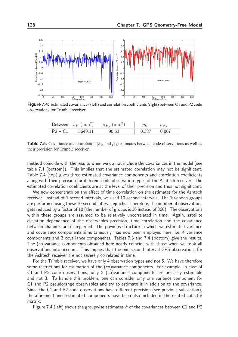
126 Chapter 7. GPS Geometry-Free Model
0 50 100 150 200 250 300 350−0.25
−0.2
−0.15
−0.1
−0.05
0
0.05
0.1
0.15
0.2
0.25
10−Epoch Group
Covariance b
etw
een P
2 a
nd C
1
mean=0.0628
0 50 100 150 200 250 300 350−1
−0.8
−0.6
−0.4
−0.2
0
0.2
0.4
0.6
0.8
1
10−Epoch Group
Co
rre
latio
n b
etw
ee
n P
2 a
nd
C1
mean=0.4399
Figure 7.4: Estimated covariances (left) and correlation coefficients (right) between C1 and P2 code
observations for Trimble receiver.
Between σij (mm2) σσij(mm2) ρij σρij
P2 – C1 5649.11 90.53 0.387 0.007
Table 7.5: Covariance and correlation (σij and ρij) estimates between code observations as well as
their precision for Trimble receiver.
method coincide with the results when we do not include the covariances in the model (seetable 7.1 (bottom)). This implies that the estimated correlation may not be significant.Table 7.4 (top) gives three estimated covariance components and correlation coefficientsalong with their precision for different code observation types of the Ashtech receiver. Theestimated correlation coefficients are at the level of their precision and thus not significant.
We now concentrate on the effect of time correlation on the estimates for the Ashtechreceiver. Instead of 1 second intervals, we used 10 second intervals. The 10-epoch groupsare performed using these 10-second interval epochs. Therefore, the number of observationsgets reduced by a factor of 10 (the number of groups is 36 instead of 360). The observationswithin these groups are assumed to be relatively uncorrelated in time. Again, satelliteelevation dependence of the observables precision, time correlation and the covariancebetween channels are disregarded. The previous structure in which we estimated varianceand covariance components simultaneously, has now been employed here, i.e. 4 variancecomponents and 3 covariance components. Tables 7.3 and 7.4 (bottom) give the results.The (co)variance components obtained here nearly coincide with those when we took allobservations into account. This implies that the one-second interval GPS observations forthe Ashtech receiver are not severely correlated in time.
For the Trimble receiver, we have only 4 observation types and not 5. We have thereforesome restrictions for estimation of the (co)variance components. For example, in case ofC1 and P2 code observations, only 2 (co)variance components are precisely estimableand not 3. To handle this problem, one can consider only one variance component forC1 and P2 pseudorange observables and try to estimate it in addition to the covariance.Since the C1 and P2 code observations have different precision (see previous subsection),the aforementioned estimated components have been also included in the related cofactormatrix.
Figure 7.4 (left) shows the groupwise estimates σ of the covariances between C1 and P2
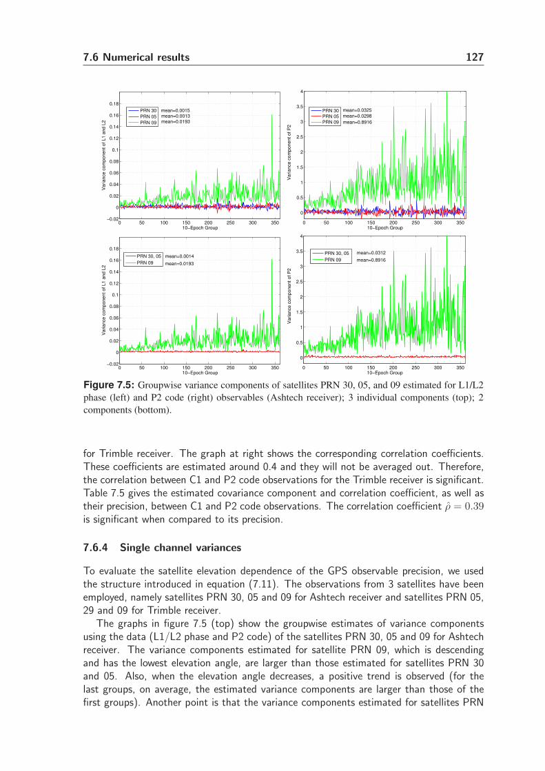
7.6 Numerical results 127
0 50 100 150 200 250 300 350−0.02
0
0.02
0.04
0.06
0.08
0.1
0.12
0.14
0.16
0.18
10−Epoch Group
Variance c
om
ponent of L1 a
nd L
2
mean=0.0015 mean=0.0013 mean=0.0193
PRN 30
PRN 05
PRN 09
0 50 100 150 200 250 300 350
0
0.5
1
1.5
2
2.5
3
3.5
4
10−Epoch Group
Variance c
om
ponent of P
2
mean=0.0325
mean=0.0298
mean=0.8916
PRN 30
PRN 05
PRN 09
0 50 100 150 200 250 300 350−0.02
0
0.02
0.04
0.06
0.08
0.1
0.12
0.14
0.16
0.18
10−Epoch Group
Variance c
om
ponent of L1 a
nd L
2
mean=0.0014
mean=0.0193
PRN 30, 05
PRN 09
0 50 100 150 200 250 300 350
0
0.5
1
1.5
2
2.5
3
3.5
4
10−Epoch Group
Va
ria
nce
co
mp
on
en
t o
f P
2
mean=0.0312
mean=0.8916
PRN 30, 05
PRN 09
Figure 7.5: Groupwise variance components of satellites PRN 30, 05, and 09 estimated for L1/L2
phase (left) and P2 code (right) observables (Ashtech receiver); 3 individual components (top); 2
components (bottom).
for Trimble receiver. The graph at right shows the corresponding correlation coefficients.These coefficients are estimated around 0.4 and they will not be averaged out. Therefore,the correlation between C1 and P2 code observations for the Trimble receiver is significant.Table 7.5 gives the estimated covariance component and correlation coefficient, as well astheir precision, between C1 and P2 code observations. The correlation coefficient ρ = 0.39is significant when compared to its precision.
7.6.4 Single channel variances
To evaluate the satellite elevation dependence of the GPS observable precision, we usedthe structure introduced in equation (7.11). The observations from 3 satellites have beenemployed, namely satellites PRN 30, 05 and 09 for Ashtech receiver and satellites PRN 05,29 and 09 for Trimble receiver.
The graphs in figure 7.5 (top) show the groupwise estimates of variance componentsusing the data (L1/L2 phase and P2 code) of the satellites PRN 30, 05 and 09 for Ashtechreceiver. The variance components estimated for satellite PRN 09, which is descendingand has the lowest elevation angle, are larger than those estimated for satellites PRN 30and 05. Also, when the elevation angle decreases, a positive trend is observed (for thelast groups, on average, the estimated variance components are larger than those of thefirst groups). Another point is that the variance components estimated for satellites PRN
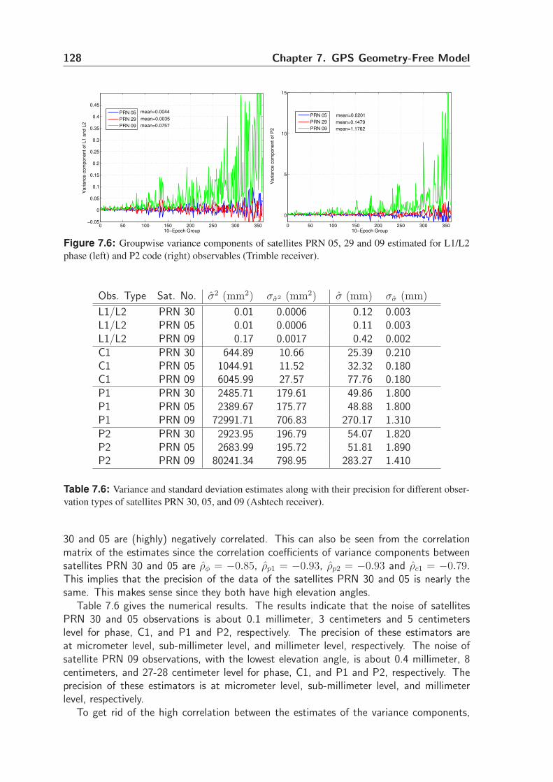
128 Chapter 7. GPS Geometry-Free Model
0 50 100 150 200 250 300 350−0.05
0
0.05
0.1
0.15
0.2
0.25
0.3
0.35
0.4
0.45
10−Epoch Group
Variance c
om
ponent of L1 a
nd L
2
mean=0.0044
mean=0.0035
mean=0.0757
PRN 05
PRN 29
PRN 09
0 50 100 150 200 250 300 350
0
5
10
15
10−Epoch Group
Variance c
om
ponent of P
2
mean=0.0201
mean=0.1479
mean=1.1762
PRN 05
PRN 29
PRN 09
Figure 7.6: Groupwise variance components of satellites PRN 05, 29 and 09 estimated for L1/L2
phase (left) and P2 code (right) observables (Trimble receiver).
Obs. Type Sat. No. σ2 (mm2) σσ2 (mm2) σ (mm) σσ (mm)
L1/L2 PRN 30 0.01 0.0006 0.12 0.003L1/L2 PRN 05 0.01 0.0006 0.11 0.003L1/L2 PRN 09 0.17 0.0017 0.42 0.002C1 PRN 30 644.89 10.66 25.39 0.210C1 PRN 05 1044.91 11.52 32.32 0.180C1 PRN 09 6045.99 27.57 77.76 0.180P1 PRN 30 2485.71 179.61 49.86 1.800P1 PRN 05 2389.67 175.77 48.88 1.800P1 PRN 09 72991.71 706.83 270.17 1.310P2 PRN 30 2923.95 196.79 54.07 1.820P2 PRN 05 2683.99 195.72 51.81 1.890P2 PRN 09 80241.34 798.95 283.27 1.410
Table 7.6: Variance and standard deviation estimates along with their precision for different obser-
vation types of satellites PRN 30, 05, and 09 (Ashtech receiver).
30 and 05 are (highly) negatively correlated. This can also be seen from the correlationmatrix of the estimates since the correlation coefficients of variance components betweensatellites PRN 30 and 05 are ρφ = −0.85, ρp1 = −0.93, ρp2 = −0.93 and ρc1 = −0.79.This implies that the precision of the data of the satellites PRN 30 and 05 is nearly thesame. This makes sense since they both have high elevation angles.
Table 7.6 gives the numerical results. The results indicate that the noise of satellitesPRN 30 and 05 observations is about 0.1 millimeter, 3 centimeters and 5 centimeterslevel for phase, C1, and P1 and P2, respectively. The precision of these estimators areat micrometer level, sub-millimeter level, and millimeter level, respectively. The noise ofsatellite PRN 09 observations, with the lowest elevation angle, is about 0.4 millimeter, 8centimeters, and 27-28 centimeter level for phase, C1, and P1 and P2, respectively. Theprecision of these estimators is at micrometer level, sub-millimeter level, and millimeterlevel, respectively.
To get rid of the high correlation between the estimates of the variance components,
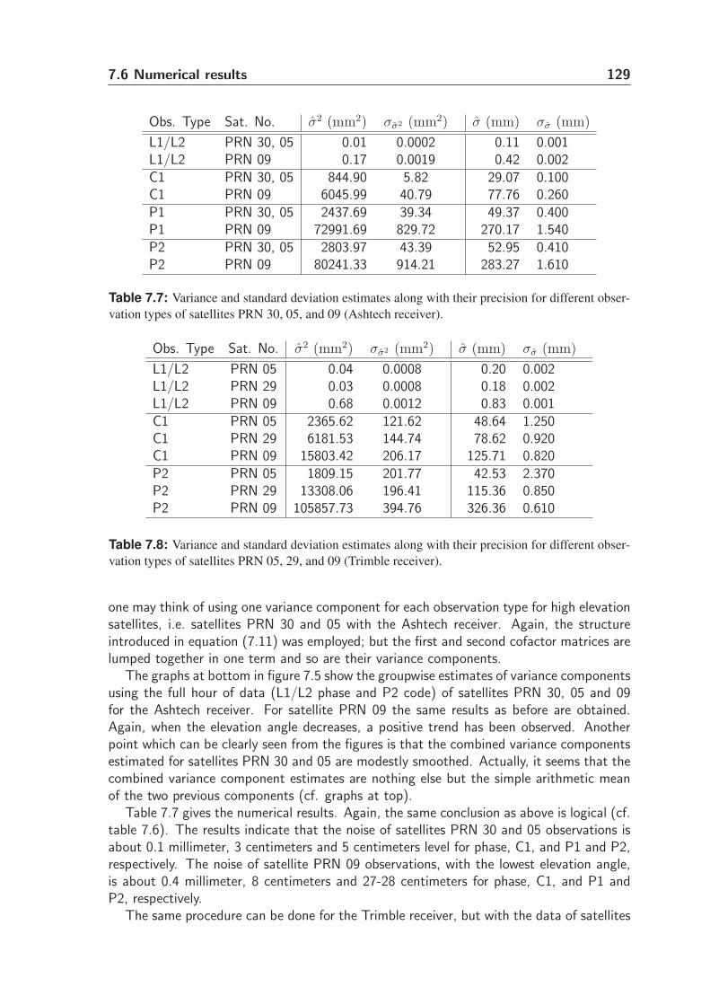
7.6 Numerical results 129
Obs. Type Sat. No. σ2 (mm2) σσ2 (mm2) σ (mm) σσ (mm)
L1/L2 PRN 30, 05 0.01 0.0002 0.11 0.001L1/L2 PRN 09 0.17 0.0019 0.42 0.002C1 PRN 30, 05 844.90 5.82 29.07 0.100C1 PRN 09 6045.99 40.79 77.76 0.260P1 PRN 30, 05 2437.69 39.34 49.37 0.400P1 PRN 09 72991.69 829.72 270.17 1.540P2 PRN 30, 05 2803.97 43.39 52.95 0.410P2 PRN 09 80241.33 914.21 283.27 1.610
Table 7.7: Variance and standard deviation estimates along with their precision for different obser-
vation types of satellites PRN 30, 05, and 09 (Ashtech receiver).
Obs. Type Sat. No. σ2 (mm2) σσ2 (mm2) σ (mm) σσ (mm)
L1/L2 PRN 05 0.04 0.0008 0.20 0.002L1/L2 PRN 29 0.03 0.0008 0.18 0.002L1/L2 PRN 09 0.68 0.0012 0.83 0.001C1 PRN 05 2365.62 121.62 48.64 1.250C1 PRN 29 6181.53 144.74 78.62 0.920C1 PRN 09 15803.42 206.17 125.71 0.820P2 PRN 05 1809.15 201.77 42.53 2.370P2 PRN 29 13308.06 196.41 115.36 0.850P2 PRN 09 105857.73 394.76 326.36 0.610
Table 7.8: Variance and standard deviation estimates along with their precision for different obser-
vation types of satellites PRN 05, 29, and 09 (Trimble receiver).
one may think of using one variance component for each observation type for high elevationsatellites, i.e. satellites PRN 30 and 05 with the Ashtech receiver. Again, the structureintroduced in equation (7.11) was employed; but the first and second cofactor matrices arelumped together in one term and so are their variance components.
The graphs at bottom in figure 7.5 show the groupwise estimates of variance componentsusing the full hour of data (L1/L2 phase and P2 code) of satellites PRN 30, 05 and 09for the Ashtech receiver. For satellite PRN 09 the same results as before are obtained.Again, when the elevation angle decreases, a positive trend has been observed. Anotherpoint which can be clearly seen from the figures is that the combined variance componentsestimated for satellites PRN 30 and 05 are modestly smoothed. Actually, it seems that thecombined variance component estimates are nothing else but the simple arithmetic meanof the two previous components (cf. graphs at top).
Table 7.7 gives the numerical results. Again, the same conclusion as above is logical (cf.table 7.6). The results indicate that the noise of satellites PRN 30 and 05 observations isabout 0.1 millimeter, 3 centimeters and 5 centimeters level for phase, C1, and P1 and P2,respectively. The noise of satellite PRN 09 observations, with the lowest elevation angle,is about 0.4 millimeter, 8 centimeters and 27-28 centimeters for phase, C1, and P1 andP2, respectively.
The same procedure can be done for the Trimble receiver, but with the data of satellites
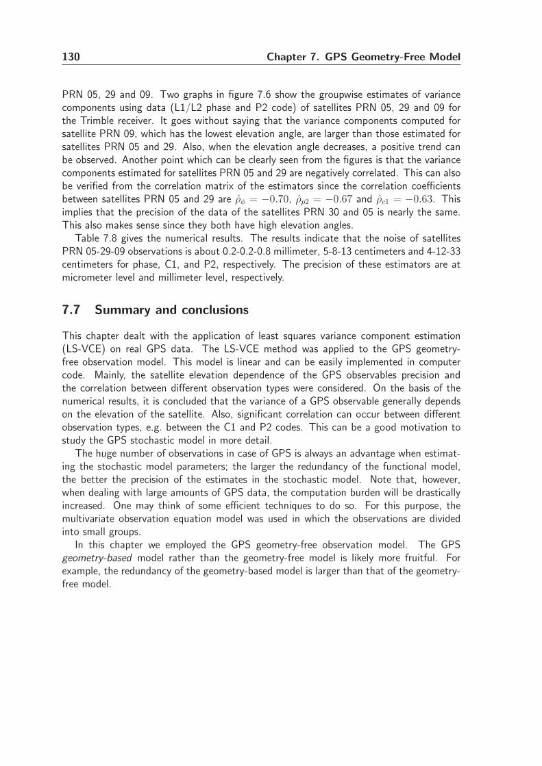
130 Chapter 7. GPS Geometry-Free Model
PRN 05, 29 and 09. Two graphs in figure 7.6 show the groupwise estimates of variancecomponents using data (L1/L2 phase and P2 code) of satellites PRN 05, 29 and 09 forthe Trimble receiver. It goes without saying that the variance components computed forsatellite PRN 09, which has the lowest elevation angle, are larger than those estimated forsatellites PRN 05 and 29. Also, when the elevation angle decreases, a positive trend canbe observed. Another point which can be clearly seen from the figures is that the variancecomponents estimated for satellites PRN 05 and 29 are negatively correlated. This can alsobe verified from the correlation matrix of the estimators since the correlation coefficientsbetween satellites PRN 05 and 29 are ρφ = −0.70, ρp2 = −0.67 and ρc1 = −0.63. Thisimplies that the precision of the data of the satellites PRN 30 and 05 is nearly the same.This also makes sense since they both have high elevation angles.
Table 7.8 gives the numerical results. The results indicate that the noise of satellitesPRN 05-29-09 observations is about 0.2-0.2-0.8 millimeter, 5-8-13 centimeters and 4-12-33centimeters for phase, C1, and P2, respectively. The precision of these estimators are atmicrometer level and millimeter level, respectively.
7.7 Summary and conclusions
This chapter dealt with the application of least squares variance component estimation(LS-VCE) on real GPS data. The LS-VCE method was applied to the GPS geometry-free observation model. This model is linear and can be easily implemented in computercode. Mainly, the satellite elevation dependence of the GPS observables precision andthe correlation between different observation types were considered. On the basis of thenumerical results, it is concluded that the variance of a GPS observable generally dependson the elevation of the satellite. Also, significant correlation can occur between differentobservation types, e.g. between the C1 and P2 codes. This can be a good motivation tostudy the GPS stochastic model in more detail.
The huge number of observations in case of GPS is always an advantage when estimat-ing the stochastic model parameters; the larger the redundancy of the functional model,the better the precision of the estimates in the stochastic model. Note that, however,when dealing with large amounts of GPS data, the computation burden will be drasticallyincreased. One may think of some efficient techniques to do so. For this purpose, themultivariate observation equation model was used in which the observations are dividedinto small groups.
In this chapter we employed the GPS geometry-free observation model. The GPSgeometry-based model rather than the geometry-free model is likely more fruitful. Forexample, the redundancy of the geometry-based model is larger than that of the geometry-free model.
GPS Coordinate Time Series 88.1 Introduction
Continuous GPS measurements have been used now nearly 15 years for estimation of crustaldeformation. Station positions are determined with respect to an earth-fixed terrestrial ref-erence system. Geophysical studies using geodetic measurements of surface displacementor strain require not only accurate estimates of these parameters but also accurate error es-timates. The precision of these estimates is often assessed by their repeatability defined bythe mean squared error of individual coordinate components (i.e. north, east, and vertical)about a linear trend. Except for the significant episodic deformation, such as large earth-quakes, a linear trend can be a good representative of the deformation behavior. The sitevelocities are usually determined by linear regression of individual coordinate components.The least-squares technique is used to estimate the line parameters, i.e. the intercept andthe slope (site velocity).
In the ideal case, it is desired that the time series possess only white noise and allfunctional effects are fully understood. The noise in GPS coordinate time series turns outnot to be white. Several geodetic data sets have provided evidence for error sources thatintroduce large temporal correlations into the data. The ultimate goal of noise-studiesis to come up with a stochastic model which allows one to process the coordinate timeseries such that the ’best’ solution (most precise solution together with proper precisiondescription) of the station positions and site velocities can be determined. An intermediategoal is therefore to better understand and identify the various noise components of thestochastic model.
Two techniques have generally been employed to assess the noise characteristics of geo-detic time series, namely the power spectral method and the maximum likelihood estimation(MLE) method. The former is aimed to examine the data in the frequency domain whilethe latter is used to examine the data covariance matrix in the time (space) domain. TheMLE can estimate the parameters of a noise model effectively in contrast to the classicalpower spectra techniques. MLE has generally been used to compute the amount of whitenoise, flicker noise and random walk noise in the time series (see e.g. Zhang et al., 1997;Langbein and Johnson, 1997; Mao et al., 1999; Williams et al., 2004; Langbein, 2004). Inthis chapter we employ the least-squares variance component estimation (LS-VCE) methodintroduced in chapters 4 and 5.
8.2 Review of previous work
Zhang et al. (1997) processed 19 months of continuous GPS coordinates from 10 sites insouthern California. Using MLE with integer spectral indices, they found that the noise in
132 Chapter 8. GPS Coordinate Time Series
the GPS time series was best described as a combination of white noise and flicker noise.This combination suggested that the velocity uncertainties should be 3-6 times larger thanthose obtained from a pure white noise model. Using the power spectra, the noise wascharacterized by a fractal noise process with a spectral index of -0.4. Neglecting thisfractal white noise model, site velocity uncertainties could be underestimated by a factorof 2-4. In an analogous way, Calais (1999); Mao et al. (1999) processed permanent GPScoordinates. They found that GPS position time series best fitted a noise model consistingof both white noise and flicker noise. In global GPS solutions, Williams et al. (2004)showed that a combination of white and flicker noise is appropriate for all three coordinatecomponents. In regional GPS solutions, the noise was substantially lower than in globalsolutions. Higher-frequency (1–30 s) GPS position time series have also been shown tocontain white plus flicker noise (Bock et al., 2000; Langbein and Bock, 2004).
Several studies have also recognized random walk noise in geodetic data. Randomwalk noise was detected in continuous measurements of strainmeters as well as very shortbaseline GPS data at Pinon Flat Observatory in southern California (Wyatt, 1982, 1989;Wyatt et al., 1989; Johnson and Agnew, 2000). Langbein and Johnson (1995, 1997) showedthat the noise in the Electronic Distance Measuring (EDM) data is well characterized bya combination of white and random walk noise. Random walk noise can be mitigated bycarefully designed monuments. GPS stations deployed in southern California for which thebase is deeply seated and laterally braced can be mentioned as a good sample (Wyattet al., 1989; Bock et al., 1997). The random walk amplitude for a very short baseline atPinon Flat Observatory is only 0.4 mm/yr1/2 (Johnson and Agnew, 2000). Beavan (2005)shows that the noise properties of GPS time series for concrete pillar monuments are verysimilar to those of deeply drilled braced monuments. Using two-color EDM measurementsin California, Langbein (2004) shows that the random walk noise model is valid for about30% of the data. In some cases a combination of random walk and band-pass-filtered noisebest characterizes the data.
Site-position time series obtained from continuous GPS arrays show significant seasonalvariations with annual and semiannual periods. Such seasonal deformation is present inboth global and regional GPS coordinate time series (see van Dam et al., 2001; Dong et al.,2002). The latter examine the nature of the observed annual and semiannual site positionvariations using 4.5 years of global continuous GPS time series. Joint contributions fromseasonal surface mass redistribution are the primary causes for the observed annual verticalvariations of site positions. Kusche and Schrama (2005) show that after removing theatmospheric pressure loading effect, estimated annual variations of continental-scale massredistribution exhibit pattern similar to those obtained with GRACE. Ding et al. (2005)used time series of daily positions of eight co-located GPS and VLBI stations to assessthe seasonal signals using the wavelet transform. Blewitt and Lavallee (2002) showedthat annual signals can significantly bias the site velocity if they are not estimated in themodel. Another important systematic error in GPS time series is the presence of offsets(jumps). Williams (2003b) discusses offset detection and estimation strategies. The effectoffset estimation has on rate uncertainty depends on the noise characteristics in the series.Kenyeres and Bruyninx (2004) estimate offsets for coordinate time series in the EUREFpermanent network. Perfetti (2006) applies the Detection Identification Adaptation (DIA)procedure, suggested by Teunissen (2000b), to permanent GPS time series to detect jumpsand to reject outliers.
This study differs in several ways from previous work. We use the least-squares variance
8.3 Analysis of GPS coordinate time series 133
component estimation (LS-VCE) method which has attractive and unique features thatwe pointed out earlier. First, LS-VCE is generally applicable and can cope with any typeof noise (and with any number of noise components) in the data series. The methodcan be implemented in a relatively simple and straightforward manner. Second, using LS-VCE one can obtain the covariance matrix of the estimators describing the uncertainty ofthe (co)variance components. Third, the LS-VCE method is employed to estimate timecorrelation assuming that the time series are stationary in time. Fourth, we use the w-teststatistic with which one can simply test the ‘contribution’ of single noise components. Onecan thus determine which noise combination is best describing the noise characteristicsof GPS position time series. In the same framework as LS-VCE we then introduce theleast-squares harmonic estimation (LS-HE) method. The goal is to introduce harmonicfunctions to capture unmodelled effects in the time series. It is then shown that practicallyonly white noise remains which is very attractive from the data processing point of view.Such a duality between the stochastic and functional model is useful to correctly judge onthe amount and behavior of noise.
8.3 Analysis of GPS coordinate time series
This section demonstrates how to estimate the time correlation of GPS coordinate timeseries using LS-VCE. We rely on a commonly accepted structure of the functional andstochastic model. To see an application of LS-VCE, time correlation of a time series isestimated using a simple expression.
8.3.1 Introduction to noise process
The power spectra, Py, of many geophysical phenomena, including the noise in GPS posi-tion time series, are well approximated as a power-law process (Mandelbrot, 1983; Agnew,1992; Mao et al., 1999; Williams, 2003a; Williams et al., 2004). The one dimensional timebehavior of the stochastic process is such that its power spectrum has the form
Py(f) = P0
(f
f0
)κ
(8.1)
where f is the temporal frequency, P0 and f0 are normalizing constants, and κ is thespectral index (see e.g. Mandelbrot and van Ness, 1968). Typical spectral index valueslie within [−3, 1]; for stationary processes −1 < κ < 1 and for non-stationary processes−3 < κ < −1. A smaller spectral index implies a more correlated process and morerelative power at lower frequencies. Special cases within this stochastic process occur atthe integer values for κ. Classical white noise has a spectral index of 0, flicker noise hasa spectral index of -1, and a random walk noise has a spectral index of -2. The powerspectral method can be employed to assess the noise characteristic of GPS time series.
The second way is to use (co)variance component estimation (VCE) methods. Therole of the data series covariance matrix is considered to be an important element withrespect to the quality criteria of the unknown parameters. Therefore, VCE methods areof great importance. There are many different methods for VCE. For more informationon VCE methods and their applications we refer to chapter 3. The noise componentsof GPS coordinate time-series, i.e. white noise, flicker noise and random walk noise, are
134 Chapter 8. GPS Coordinate Time Series
usually estimated by the MLE method which is a well-known estimation principle. The MLEproblem can be solved in several ways (see Kubik, 1970; Koch, 1986; Ou, 1989; Yu, 1996;Grodecki, 1999, 2001). In time series analysis of GPS coordinates, the MLE is describedby Langbein and Johnson (1997), Zhang et al. (1997), Mao et al. (1999), Calais (1999),and Williams et al. (2004). They all selected the downhill simplex method developed byNelder and Mead (Press et al., 1992). Using expressions given by Sahin et al. (1992), someauthors used a simplified algorithm for VCE (see Davies and Blewitt, 2000; Altamimi et al.,2002).
In contrast to MLE which gives biased estimators, LS-VCE provides unbiased and min-imum variance estimators. The unbiasedness property is independent of the (unspecified)distribution of the data. LS-VCE is also faster than MLE since it iterates in a Newton-Raphson scheme towards a solution rather than using the downhill simplex which can beextremely slow (see Press et al., 1992). Another advantage of LS-VCE over downhill sim-plex method is the possibility of incorporating any number of noise components in thestochastic model. Using hypothesis testing one can also simply judge in an objective man-ner which noise components are likely to be present in the series (see sections 8.4.2 and8.5.4.2).
8.3.2 Functional model
We restrict ourselves to the problem of time correlation estimation for an individual com-ponent of GPS coordinate time series. In functional model E{y} = Ax, y is the m-vectorof time series observations, e.g. daily GPS positions of one component. Hereinafter itis denoted by y(t) where t refers to the time instant. When a linear trend describes thedeformation behavior, the functional model will read: E{y(t)} = y0 + r t. When there arein addition q periodic signals in the data series, the functional model is extended to
E{y(t)} = y0 + r t +
q∑
k=1
ak cos ωkt + bk sin ωkt (8.2)
Two trigonometrical terms cos and sin together represent a sinusoidal wave with in generala non-zero initial phase. The structure introduced above has the advantage of being linear.The unknown vector x consists of the intercept y0, the slope r and the coefficients ak andbk. In case of a linear trend and annual and semiannual signals (q = 2), the design matrixA is of size m× 6. Its ith row at time instant ti is given as
ai = [1 ti cos 2πti sin 2πti cos 4πti sin 4πti] (8.3)
where ti is expressed in terms of year (yr). In section 8.4.1 we show how to obtain anappropriate functional model.
8.3.3 Stochastic model
If the time series of GPS coordinates is composed of white noise, flicker noise, and randomwalk noise with variances σ2
w, σ2f , and σ2
rw, respectively, the covariance matrix of the timeseries can then be written as (Q0 = 0)
Qy = σ2wI + σ2
fQf + σ2rwQrw (8.4)
8.3 Analysis of GPS coordinate time series 135
where I is the m×m identity matrix, and Qf and Qrw are the cofactor matrices relatingto flicker noise and random walk noise, respectively. The structure of Qy matrix is knownthrough I, Qf , and Qrw, but the contributions through σw, σf , and σrw are unknown. Insection 8.4.2 we show how to improve an existing stochastic model.
The elements of the flicker noise cofactor matrix Qf can be approximated by (Zhanget al., 1997)
q(f)ij =
{98
if τ = 098
(
1− log τ/log 2+224
)
if τ 6= 0(8.5)
where τ = |tj − ti|. For evenly spaced data, the matrix Qf is a symmetric Toeplitz matrixwhich contains constant values along negative-sloping diagonals. It is important to notethat the Hosking flicker noise covariance matrix which was introduced and used by Williams(2003a); Langbein (2004); Williams et al. (2004); Beavan (2005) can also be used. Themain difference is a scaling of the amplitudes. Therefore, the flicker noise variances we usehere are roughly one-half the size of those quoted in these papers.
A random walk process is derived by integrating white noise. Random walk noise issupposed to be zero at initial time t0 . For evenly spaced data, the random walk cofactormatrix Qrw is expressed as
Qrw = f−1s
1 1 · · · 11 2 · · · 2...
.... . .
...1 2 · · · m
; fs =m− 1
T(8.6)
where fs is the sampling frequency in yr−1, and T is the total observation span (Johnsonand Wyatt, 1994; Zhang et al., 1997; Mao et al., 1999).
The variance components σ2w, σ2
f and σ2rw can now be estimated using the LS-VCE
method.
8.3.4 Misspecification in functional and stochastic model
A discussion on the misspecifications (errors) in the functional and stochastic model is inplace as in practice man’s models of real phenomena will always be misspecified. Concerningthe number of parameters in a model two types of misspecifications can occur: overpara-metrization and underparameterization. Underparametrization in the functional model willgenerally lead to biases in the estimation of x and thus in the results of variance componentestimation (aliasing) for noise assessment. The side effect of underparameterization in thefunctional model can also be a misinterpretation in terms of underparameterization in thestochastic model (see section 8.4.3). Overparametrization in general does not introducebiases provided the remaining redundancy is such that sufficiently precise estimates of x(and thus VCE-results) can be obtained. If however overparametrization in the functionalmodel can seriously affect the noise amplitudes in the stochastic model, this simply meansthat the extended part of the functional model is closely related to the stochastic model.One can therefore expect to see a duality between the functional and stochastic model.
Misspecifications in the stochastic model will not lead to biases in the estimation of x(after all weighted least-squares is still unbiased). However, underparameterization in the
136 Chapter 8. GPS Coordinate Time Series
stochastic model leads to biases in (co)variance components. This will result in an incorrectprecision description of the estimator x (also losing the ‘best’ property). To discuss theeffect of misspecifications (in fact underparameterization) in the stochastic model, let Qy
be the correct covariance matrix and Q′y be an incorrect one. If least-squares estimation of
x is done with Q′y, then x = (AT Q′−1
y A)−1AT Q′−1y y is still an unbiased estimator of x and
Qx = (AT Q′−1y A)−1AT Q′−1
y QyQ′−1y A(AT Q′−1
y A)−1 (8.7)
is the correct covariance matrix of the estimator x. Therefore, if one uses Q′x =
(AT Q′−1y A)−1 as the matrix to describe the precision of x one will have an incorrect
precision description which can be too optimistic if Qx ≥ Q′x, but also too pessimistic if
Qx ≤ Q′x. Comparisons of precision description of estimates for different stochastic models
are given in section 8.5.6.
8.4 Model identification
8.4.1 Least-squares harmonic estimation (LS-HE)
In this subsection it is aimed to determine an adequate design matrix A for the functionalmodel through parameter significance testing. For a time series yT = [y
1, y
2, ..., y
m] defined
on Rm, we assume that it can be expressed as a linear trend plus a sum of q individual
trigonometric terms, i.e. E{y(t)} = y0 + r t +∑q
k=1 ak cos ωkt + bk sin ωkt (see equation(8.2)). In matrix notation, we may write
E{y} = Ax +
q∑
k=1
Akxk, D{y} = Qy (8.8)
where the design matrix A contains for instance two columns of the linear regression termsand the matrix Ak consists of two columns corresponding to the frequency ωk of thesinusoidal function
Ak =
cos ωkt1 sin ωkt1cos ωkt2 sin ωkt2
......
cos ωktm sin ωktm
and xk =
[ak
bk
]
(8.9)
with ak, bk and ωk being (un)known real numbers. On the one hand, if the frequencies ωk
are known, one will deal with the most popular (linear) least-squares problem to estimateamplitudes ak and bk’s. Petrov and Ma (2003) studied harmonic position variations of 40VLBI stations at 32 known tidal frequencies. They found that the estimates of stationdisplacements generally agree with the ocean loading computed on the basis of modernocean tide models for the main diurnal and semidiurnal tides. On the other hand, if thefrequencies ωk are unknown, the problem of finding these unknown parameters is the taskof least-squares harmonic estimation.
The problem now is to find the set of frequencies ω1, · · · , ωq, and in particular the valueq, in equation (8.8). The following null and alternative hypotheses are put forward (tostart, set i = 1):
Ho : E{y} = Ax +i−1∑
k=1
Akxk (8.10)
8.4 Model identification 137
versus
Ha : E{y} = Ax +i∑
k=1
Akxk (8.11)
The detection and validation of ωi is completed through the following two steps:
Step I The goal is to find the frequency ωi (and correspondingly Ai) by solving thefollowing minimization problem:
ωi =arg minωj
||P⊥[A Aj ]
y||2Q−1
y=arg min
ωj
||ea||2Q−1y
(8.12)
where ||.||2Q−1
y= (.)T Q−1
y (.), A = [A A1 ... Ai−1] and ea is the least-squares residuals under
the alternative hypothesis. The matrix Aj has the same structure as Ak in equation (8.9);the one which minimizes the preceding criterion is set to be Ai. The above minimizationproblem is equivalent to the following maximization problem (Teunissen, 2000a, p. 96):
ωi = arg maxωj
||PAjy||2
Q−1y
, with Aj = P⊥A
Aj (8.13)
with PAj= Aj(A
T
j Q−1y Aj)
−1AT
j Q−1y . The preceding equation simplifies to
ωi =arg maxωj
eT0 Q−1
y Aj(ATj Q−1
y P⊥A
Aj)−1AT
j Q−1y e0 (8.14)
with e0 = P⊥A
y the least-squares residuals under the null hypothesis. In the case that thetime series contains only white noise, namely Qy = σ2I, it follows that
ωi = arg maxωj
eT0 Aj(A
Tj P⊥
AAj)
−1ATj e0 (8.15)
Analytical evaluation of the above maximization problem is complicated. In practice,one has to be satisfied with numerical evaluation. A plot of spectral values ||PAj
y||2Q−1
y
versus a set of discrete values for ωj can be used as a tool to investigate the contributionof different frequencies in the construction of the original time series. That is, we cancompute the spectral values for different frequencies using equation (8.14) or (8.15). Thefrequency at which ||PAj
y||2Q−1
yachieves its maximum value is used to construct Ai.
Step II To test Ho against Ha in equation (8.11), we consider Qy = σ2I, with σ2 unknown.The following test statistic can be used (see Teunissen et al., 2005)
T 2 =||PAi
y||2Q−1
y
2σ2a
=eT0 Ai(A
Ti P⊥
AAi)
−1ATi e0
2σ2a
(8.16)
where Ai = P⊥A
Ai and the estimator for the variance, σ2a, has to be computed under the
alternative hypothesis. Under Ho, the test statistic has a central Fisher distribution
T 2 ∼ F(2,m− n− 2i) (8.17)
The above hypothesis testing is in fact the parameter significance test because the teststatistic T 2 can also be expressed in terms of xi in equation (8.11) and its covariance matrix.
138 Chapter 8. GPS Coordinate Time Series
If the null hypothesis is rejected, we can increase i by one step and perform the sameprocedure for finding yet another frequency. As a generalization of the Fourier SpectralAnalysis, the method is neither limited to evenly spaced data nor to integer frequencies.
When measuring a functionally known quantity, equation (8.15) reads ωi =arg maxωj
eT0 Aj(A
Tj Aj)
−1ATj e0 which is identical to the least-squares spectral analysis
(LSSA) method developed by Vanıcek (1969). For some applications refer to Craymer(1998); Abbasi (1999); Asgari and Harmel (2005); Amiri-Simkooei (2005). Amiri-Simkooeiand Tiberius (2007) assess the noise characteristics of GPS receivers using zero-baselinetime series and arrive at the same conclusions using short-baseline time series when mul-tipath effects were captured by a set of harmonic functions. With equations (8.8)–(8.11)and (8.14) we now have a formulation for LSSA even when an initial design matrix A ispresent in the model and the covariance matrix Qy, in general, is not a scaled identitymatrix.
Our application of harmonic estimation, in the first place, is to find any potential peri-odicities in the series. The remaining unmodelled effects (e.g. power-law noise) will alsobe interpreted and captured by a set of harmonic functions. Once we compensate for theseeffects in the functional model, the remaining noise characteristics of the series will beassessed. A nearly white noise combined with autoregressive noise can be shown to remainin the data series. This will bring us to see a duality between the stochastic and functionalmodel; what is not captured in the functional model is captured in the stochastic modeland vice versa.
8.4.2 The w-test statistic
Here we aim to determine the appropriate covariance matrix Qy through significance testingon the stochastic model. One advantage of LS-VCE over other methods is that one can usestatistical hypothesis testing in the stochastic model (similar as done with the functionalmodel). When there is no misspecification in the functional part of the model E{y} = Ax,the following two hypotheses, as an example, are taken into account:
Ho : Qy = σ2wI versus Ha : Qy = σ2
wI + Cy∇ (8.18)
where Cy is a known cofactor matrix, for example Qf or Qrw, and ∇ is an unknown(co)variance parameter. We can use the generalized likelihood ratio test for testing Ho
against Ha. The following w-test statistic can be obtained from equation (5.81), withQy = σ2
wI
w =b eT Cye− tr(CyP
⊥A )eT e
σ2w
[2b2 tr(CyP⊥
A CyP⊥A )− 2b tr(CyP⊥
A )2]1/2
(8.19)
with b = m− n the redundancy of the functional model and e the least-squares residualsunder the null hypothesis.
The expectation and the variance of the w-test statistic are zero and one, respectively(see equations (5.42) and (5.49)). The distribution of this statistic, for large m, can beapproximated by the standard normal distribution. The goal now is to compute the w-test statistic values for different alternative hypotheses, i.e. different Cy’s in the precedingequation, and select the one that gives the maximum value for the w-test. In fact, equation(8.19) provides us with an objective measure to judge, whether or not (or which), additional
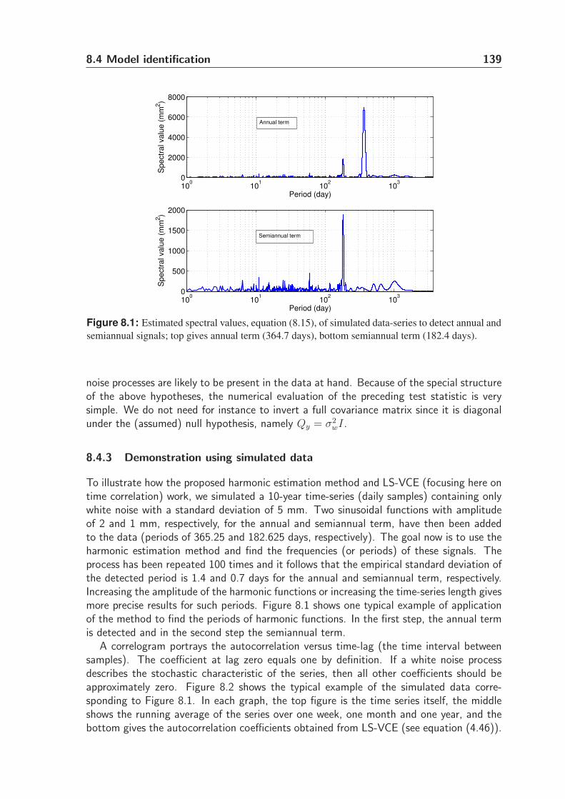
8.4 Model identification 139
100
101
102
103
0
2000
4000
6000
8000
Period (day)
Sp
ectr
al va
lue
(m
m2)
100
101
102
103
0
500
1000
1500
2000
Period (day)
Sp
ectr
al va
lue
(m
m2)
Annual term
Semiannual term
Figure 8.1: Estimated spectral values, equation (8.15), of simulated data-series to detect annual and
semiannual signals; top gives annual term (364.7 days), bottom semiannual term (182.4 days).
noise processes are likely to be present in the data at hand. Because of the special structureof the above hypotheses, the numerical evaluation of the preceding test statistic is verysimple. We do not need for instance to invert a full covariance matrix since it is diagonalunder the (assumed) null hypothesis, namely Qy = σ2
wI.
8.4.3 Demonstration using simulated data
To illustrate how the proposed harmonic estimation method and LS-VCE (focusing here ontime correlation) work, we simulated a 10-year time-series (daily samples) containing onlywhite noise with a standard deviation of 5 mm. Two sinusoidal functions with amplitudeof 2 and 1 mm, respectively, for the annual and semiannual term, have then been addedto the data (periods of 365.25 and 182.625 days, respectively). The goal now is to use theharmonic estimation method and find the frequencies (or periods) of these signals. Theprocess has been repeated 100 times and it follows that the empirical standard deviation ofthe detected period is 1.4 and 0.7 days for the annual and semiannual term, respectively.Increasing the amplitude of the harmonic functions or increasing the time-series length givesmore precise results for such periods. Figure 8.1 shows one typical example of applicationof the method to find the periods of harmonic functions. In the first step, the annual termis detected and in the second step the semiannual term.
A correlogram portrays the autocorrelation versus time-lag (the time interval betweensamples). The coefficient at lag zero equals one by definition. If a white noise processdescribes the stochastic characteristic of the series, then all other coefficients should beapproximately zero. Figure 8.2 shows the typical example of the simulated data corre-sponding to Figure 8.1. In each graph, the top figure is the time series itself, the middleshows the running average of the series over one week, one month and one year, and thebottom gives the autocorrelation coefficients obtained from LS-VCE (see equation (4.46)).
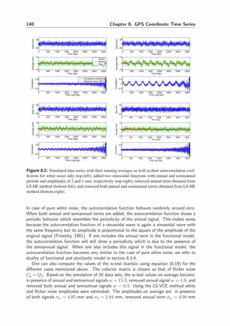
140 Chapter 8. GPS Coordinate Time Series
0 500 1000 1500 2000 2500 3000 3500
−20
0
20
Time (day)
Da
ta (
mm
)
0 500 1000 1500 2000 2500 3000 3500−10
0
10
Time (day)
Ave
rag
e (
mm
)
0 500 1000 1500 2000 2500 3000 3500
−0.2
0
0.2
Time−Lag (day)
Co
rre
latio
n Correlation coefficient
Maximum error (95%)
Week
Month
Year
0 500 1000 1500 2000 2500 3000 3500
−20
0
20
Time (day)
Da
ta (
mm
)
0 500 1000 1500 2000 2500 3000 3500−10
0
10
Time (day)
Ave
rag
e (
mm
)
0 500 1000 1500 2000 2500 3000 3500
−0.2
0
0.2
Time−Lag (day)
Co
rre
latio
n0 500 1000 1500 2000 2500 3000 3500
−20
0
20
Time (day)
Da
ta (
mm
)
0 500 1000 1500 2000 2500 3000 3500−10
0
10
Time (day)
Ave
rag
e (
mm
)
0 500 1000 1500 2000 2500 3000 3500
−0.2
0
0.2
Time−Lag (day)
Co
rre
latio
n
0 500 1000 1500 2000 2500 3000 3500
−20
0
20
Time (day)
Da
ta (
mm
)
0 500 1000 1500 2000 2500 3000 3500−10
0
10
Time (day)
Ave
rag
e (
mm
)
0 500 1000 1500 2000 2500 3000 3500
−0.2
0
0.2
Time−Lag (day)
Co
rre
latio
n
Figure 8.2: Simulated data-series with their running averages as well as their autocorrelation coef-
ficients for white noise only (top-left); added two sinusoidal functions with annual and semiannual
periods and amplitudes of 2 and 1 mm, respectively (top-right); removed annual term obtained from
LS-HE method (bottom-left); and removed both annual and semiannual terms obtained from LS-HE
method (bottom-right).
In case of pure white noise, the autocorrelation function behaves randomly around zero.When both annual and semiannual terms are added, the autocorrelation function shows aperiodic behavior which resembles the periodicity of the annual signal. This makes sensebecause the autocorrelation function of a sinusoidal wave is again a sinusoidal wave withthe same frequency but its amplitude is proportional to the square of the amplitude of theoriginal signal (Priestley, 1981). If one includes the annual term in the functional model,the autocorrelation function will still show a periodicity which is due to the presence ofthe semiannual signal. When one also includes this signal in the functional model, theautocorrelation function becomes very similar to the case of pure white noise; we refer toduality of functional and stochastic model in section 8.3.4.
One can also compute the values of the w-test statistic using equation (8.19) for thedifferent cases mentioned above. The cofactor matrix is chosen as that of flicker noiseCy = Qf . Based on the simulation of 20 data sets, the w-test values on average become:in presence of annual and semiannual signals w = 15.3, removed annual signal w = 1.9, andremoved both annual and semiannual signals w = 0.3. Using the LS-VCE method whiteand flicker noise amplitudes were estimated. The amplitudes on average are: in presenceof both signals σw = 4.85 mm and σf = 2.84 mm, removed annual term σw = 4.98 mm
8.5 Numerical results and discussions 141
and σf = 1.35, mm and removed both terms σw = 5.00 mm and σf = 0.07 mm. These alltogether simply express that if there exist unmodelled effects in data, they can mistakenlybe interpreted as time correlation (here flicker noise). One should therefore take care ofthese signals in the functional model.
8.5 Numerical results and discussions
8.5.1 Data and model description
Global time series of site positions are supposed to have more noise than those froma regional solution (Williams et al., 2004). Therefore, the daily GPS global solutions ofdifferent stations processed by the GPS Analysis Center at JPL are adopted. The data wereprocessed using the precise point positioning method in the GIPSY software (Zumbergeet al., 1997). The satellite orbits, satellite clocks and Earth rotation parameters (ERP) usedfor the daily solutions were estimated with data from 42 globally distributed IGS trackingstations (see Beutler et al., 1999). In addition, corrections for geophysical effects such aspole and ocean tide effects have been applied. The reader is referred to the JPL website[http://sideshow.jpl.nasa.gov/mbh/series.html].
The estimated coordinates of a site are uncorrelated with those of the other sites if theeffects of the common errors in the satellite orbits and clocks and ERP on the estimatedcoordinates are insignificant. To make a proper statement, one can rely on multivariatetime series analysis methods. The time series are processed component-by-component inthis chapter.
Most of the results given are based on 5 stations, namely KOSG, WSRT, ONSA, GRAZand ALGO. Four stations are in Europe of which KOSG and WSRT in the Netherlands,ONSA in Sweden, and GRAZ in Austria. ALGO is in Canada. We have used 10-years ofdaily solutions for all sites except WSRT which covers only 6.5 years. To justify some of thestatements that we will make, 71 globally distributed GPS stations were also processed. Ourpoint of departure is the original time series and its linear model of observation equationsyt = y0 + r t. In some cases, the annual and semiannual signals have been considered aswell. At times, we have included a set of harmonic functions to compensate for (parts of)unmodelled effects in the series.
8.5.2 Variance component analysis
Three stochastic models have been chosen to describe the noise characteristics of GPScoordinate time series. They include the pure white noise model (I), the white plus flickernoise model (IIa), and the white plus random walk noise model (III). We employed LS-VCE to estimate the white noise, flicker noise, and random walk noise amplitudes (seeequation (8.4)). Williams investigations (pers. commun.; Williams (2006)) show that LS-VCE gives the same results as MLE. This holds in fact if m >> n which is usually thecase in time series analysis. Table 8.1 gives the noise amplitudes of different componentsfor different stochastic models. The table also provides the precision (standard deviation)of the estimates which is an important feature of LS-VCE. We find, for different noisecomponents, that the horizontal components are less noisy than the vertical componentsby a factor of 2-4. Compared to the white noise model only, the amplitude of white noisefor the white plus flicker noise model is 30% smaller, while this reduction for white plus
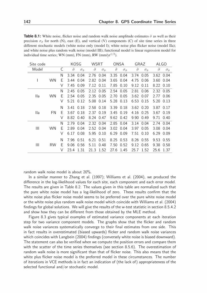
142 Chapter 8. GPS Coordinate Time Series
Table 8.1: White noise, flicker noise and random walk noise amplitude estimates σ as well as their
precision σσ for north (N), east (E), and vertical (V) components (C) of site time series in three
different stochastic models (white noise only (model I); white noise plus flicker noise (model IIa);
and white noise plus random walk noise (model III); functional model is linear regression model for
individual time series; WN (mm), FN (mm), RW (mm/yr1/2).
Site code KOSG WSRT ONSA GRAZ ALGOModel C σ σσ σ σσ σ σσ σ σσ σ σσ
N 3.34 0.04 2.76 0.04 3.35 0.04 3.74 0.05 3.62 0.04I WN E 3.44 0.04 2.82 0.04 3.65 0.04 4.75 0.06 3.60 0.04
V 7.45 0.09 7.12 0.11 7.85 0.10 9.12 0.11 8.22 0.10
N 2.45 0.05 2.12 0.05 2.54 0.05 2.81 0.06 2.32 0.05IIa WN E 2.54 0.05 2.35 0.05 2.70 0.05 3.62 0.07 2.77 0.06
V 5.21 0.12 5.08 0.14 5.28 0.13 6.53 0.15 5.20 0.13
N 3.41 0.18 2.58 0.18 3.39 0.18 3.62 0.20 3.87 0.17IIa FN E 3.67 0.18 2.37 0.19 3.45 0.19 4.16 0.25 3.67 0.19
V 8.82 0.40 8.24 0.47 9.62 0.42 9.90 0.49 9.71 0.40
N 2.79 0.04 2.32 0.04 2.85 0.04 3.14 0.04 2.74 0.04III WN E 2.89 0.04 2.52 0.04 3.02 0.04 3.97 0.05 3.08 0.04
V 6.17 0.08 5.95 0.10 6.29 0.09 7.51 0.10 6.29 0.09
N 7.96 0.51 6.21 0.51 8.25 0.53 8.26 0.55 9.53 0.55III RW E 9.06 0.56 5.11 0.48 7.50 0.52 9.12 0.65 9.38 0.58
V 23.4 1.31 21.3 1.52 27.6 1.45 25.7 1.52 25.6 1.37
random walk noise model is about 20%.In a similar manner to Zhang et al. (1997); Williams et al. (2004), we produced the
difference in the log-likelihood values for each site, each component and each error model.The results are given in Table 8.2. The values given in this table are normalized such thatthe pure white noise model has a log-likelihood of zero. These results confirm that thewhite noise plus flicker noise model seems to be preferred over the pure white noise modelor the white noise plus random walk noise model which coincide with Williams et al. (2004)findings for global solutions. We will give the results of the w-test statistic in section 8.5.4.2and show how they can be different from those obtained by the MLE method.
Figure 8.3 gives typical examples of estimated variance components at each iterationstep for two variance component models. The graphs show that the flicker and randomwalk noise variances systematically converge to their final estimates from one side. Thisin fact results in overestimated (biased upwards) flicker and random walk noise varianceswhich coincides with Langbein (2004) findings (conversely white noise is biased downward).The statement can also be verified when we compute the position errors and compare themwith the scatter of the time series themselves (see section 8.5.6). The overestimation ofrandom walk noise is more significant than that of flicker noise. This also means that thewhite plus flicker noise model is the preferred model in these circumstances. The numberof iterations in VCE methods is in fact an indication of (the lack of) appropriateness of theselected functional and/or stochastic model.
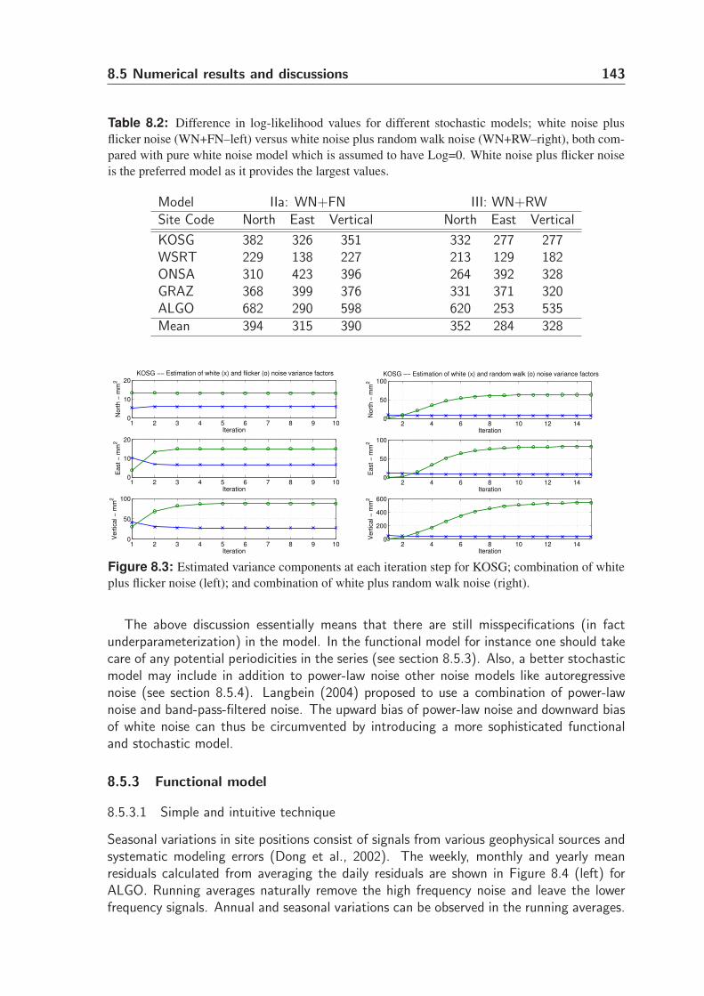
8.5 Numerical results and discussions 143
Table 8.2: Difference in log-likelihood values for different stochastic models; white noise plus
flicker noise (WN+FN–left) versus white noise plus random walk noise (WN+RW–right), both com-
pared with pure white noise model which is assumed to have Log=0. White noise plus flicker noise
is the preferred model as it provides the largest values.
Model IIa: WN+FN III: WN+RWSite Code North East Vertical North East Vertical
KOSG 382 326 351 332 277 277WSRT 229 138 227 213 129 182ONSA 310 423 396 264 392 328GRAZ 368 399 376 331 371 320ALGO 682 290 598 620 253 535Mean 394 315 390 352 284 328
1 2 3 4 5 6 7 8 9 100
10
20
Iteration
Nort
h −
mm
2
KOSG −− Estimation of white (x) and flicker (o) noise variance factors
1 2 3 4 5 6 7 8 9 100
10
20
Iteration
East −
mm
2
1 2 3 4 5 6 7 8 9 100
50
100
Iteration
Vert
ical −
mm
2
2 4 6 8 10 12 140
50
100
Iteration
Nort
h −
mm
2
KOSG −− Estimation of white (x) and random walk (o) noise variance factors
2 4 6 8 10 12 140
50
100
Iteration
East −
mm
2
2 4 6 8 10 12 140
200
400
600
Iteration
Vert
ical −
mm
2
Figure 8.3: Estimated variance components at each iteration step for KOSG; combination of white
plus flicker noise (left); and combination of white plus random walk noise (right).
The above discussion essentially means that there are still misspecifications (in factunderparameterization) in the model. In the functional model for instance one should takecare of any potential periodicities in the series (see section 8.5.3). Also, a better stochasticmodel may include in addition to power-law noise other noise models like autoregressivenoise (see section 8.5.4). Langbein (2004) proposed to use a combination of power-lawnoise and band-pass-filtered noise. The upward bias of power-law noise and downward biasof white noise can thus be circumvented by introducing a more sophisticated functionaland stochastic model.
8.5.3 Functional model
8.5.3.1 Simple and intuitive technique
Seasonal variations in site positions consist of signals from various geophysical sources andsystematic modeling errors (Dong et al., 2002). The weekly, monthly and yearly meanresiduals calculated from averaging the daily residuals are shown in Figure 8.4 (left) forALGO. Running averages naturally remove the high frequency noise and leave the lowerfrequency signals. Annual and seasonal variations can be observed in the running averages.
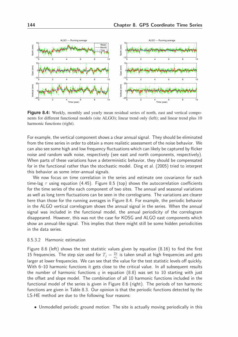
144 Chapter 8. GPS Coordinate Time Series
0 2 4 6 8 10−10
0
10
No
rth
(m
m)
ALGO −− Running average
0 2 4 6 8 10−10
0
10
Ea
st
(mm
)
0 2 4 6 8 10−20
0
20
Ve
rtic
al (m
m)
Time (year)
Week
Month
Year
0 2 4 6 8 10−10
0
10
No
rth
(m
m)
ALGO −− Running average
0 2 4 6 8 10−10
0
10
Ea
st
(mm
)
0 2 4 6 8 10−20
0
20
Ve
rtic
al (m
m)
Time (year)
Figure 8.4: Weekly, monthly and yearly mean residual series of north, east and vertical compo-
nents for different functional models (site ALGO); linear trend only (left); and linear trend plus 10
harmonic functions (right).
For example, the vertical component shows a clear annual signal. They should be eliminatedfrom the time series in order to obtain a more realistic assessment of the noise behavior. Wecan also see some high and low frequency fluctuations which can likely be captured by flickernoise and random walk noise, respectively (see east and north components, respectively).When parts of these variations have a deterministic behavior, they should be compensatedfor in the functional rather than the stochastic model. Ding et al. (2005) tried to interpretthis behavior as some inter-annual signals.
We now focus on time correlation in the series and estimate one covariance for eachtime-lag τ using equation (4.45). Figure 8.5 (top) shows the autocorrelation coefficientsfor the time series of the each component of two sites. The annual and seasonal variationsas well as long term fluctuations can be seen in the correlograms. The variations are clearerhere than those for the running averages in Figure 8.4. For example, the periodic behaviorin the ALGO vertical correlogram shows the annual signal in the series. When the annualsignal was included in the functional model, the annual periodicity of the correlogramdisappeared. However, this was not the case for KOSG and ALGO east components whichshow an annual-like signal. This implies that there might still be some hidden periodicitiesin the data series.
8.5.3.2 Harmonic estimation
Figure 8.6 (left) shows the test statistic values given by equation (8.16) to find the first15 frequencies. The step size used for Tj = 2π
ωjis taken small at high frequencies and gets
larger at lower frequencies. We can see that the value for the test statistic levels off quickly.With 6–10 harmonic functions it gets close to the critical value. In all subsequent resultsthe number of harmonic functions q in equation (8.8) was set to 10 starting with justthe offset and slope model. The combination of all 10 harmonic functions included in thefunctional model of the series is given in Figure 8.6 (right). The periods of ten harmonicfunctions are given in Table 8.3. Our opinion is that the periodic functions detected by theLS-HE method are due to the following four reasons:
• Unmodelled periodic ground motion: The site is actually moving periodically in this
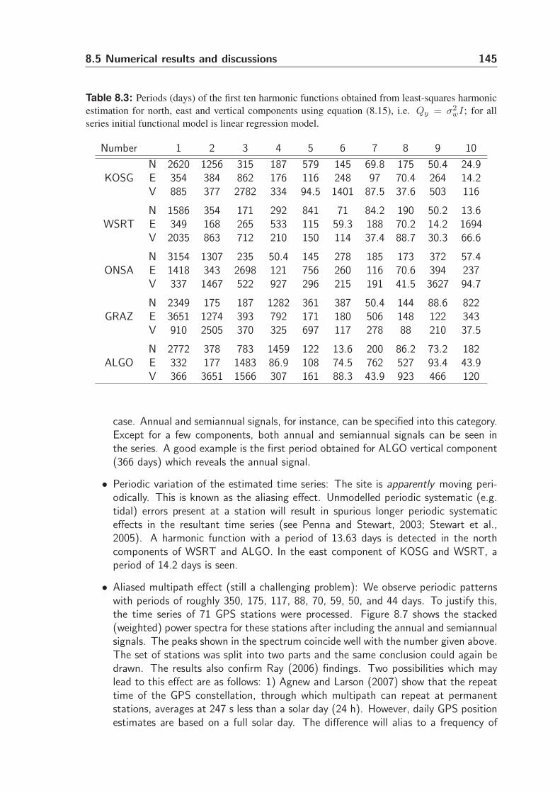
8.5 Numerical results and discussions 145
Table 8.3: Periods (days) of the first ten harmonic functions obtained from least-squares harmonic
estimation for north, east and vertical components using equation (8.15), i.e. Qy = σ2wI; for all
series initial functional model is linear regression model.
Number 1 2 3 4 5 6 7 8 9 10
N 2620 1256 315 187 579 145 69.8 175 50.4 24.9KOSG E 354 384 862 176 116 248 97 70.4 264 14.2
V 885 377 2782 334 94.5 1401 87.5 37.6 503 116
N 1586 354 171 292 841 71 84.2 190 50.2 13.6WSRT E 349 168 265 533 115 59.3 188 70.2 14.2 1694
V 2035 863 712 210 150 114 37.4 88.7 30.3 66.6
N 3154 1307 235 50.4 145 278 185 173 372 57.4ONSA E 1418 343 2698 121 756 260 116 70.6 394 237
V 337 1467 522 927 296 215 191 41.5 3627 94.7
N 2349 175 187 1282 361 387 50.4 144 88.6 822GRAZ E 3651 1274 393 792 171 180 506 148 122 343
V 910 2505 370 325 697 117 278 88 210 37.5
N 2772 378 783 1459 122 13.6 200 86.2 73.2 182ALGO E 332 177 1483 86.9 108 74.5 762 527 93.4 43.9
V 366 3651 1566 307 161 88.3 43.9 923 466 120
case. Annual and semiannual signals, for instance, can be specified into this category.Except for a few components, both annual and semiannual signals can be seen inthe series. A good example is the first period obtained for ALGO vertical component(366 days) which reveals the annual signal.
• Periodic variation of the estimated time series: The site is apparently moving peri-odically. This is known as the aliasing effect. Unmodelled periodic systematic (e.g.tidal) errors present at a station will result in spurious longer periodic systematiceffects in the resultant time series (see Penna and Stewart, 2003; Stewart et al.,2005). A harmonic function with a period of 13.63 days is detected in the northcomponents of WSRT and ALGO. In the east component of KOSG and WSRT, aperiod of 14.2 days is seen.
• Aliased multipath effect (still a challenging problem): We observe periodic patternswith periods of roughly 350, 175, 117, 88, 70, 59, 50, and 44 days. To justify this,the time series of 71 GPS stations were processed. Figure 8.7 shows the stacked(weighted) power spectra for these stations after including the annual and semiannualsignals. The peaks shown in the spectrum coincide well with the number given above.The set of stations was split into two parts and the same conclusion could again bedrawn. The results also confirm Ray (2006) findings. Two possibilities which maylead to this effect are as follows: 1) Agnew and Larson (2007) show that the repeattime of the GPS constellation, through which multipath can repeat at permanentstations, averages at 247 s less than a solar day (24 h). However, daily GPS positionestimates are based on a full solar day. The difference will alias to a frequency of
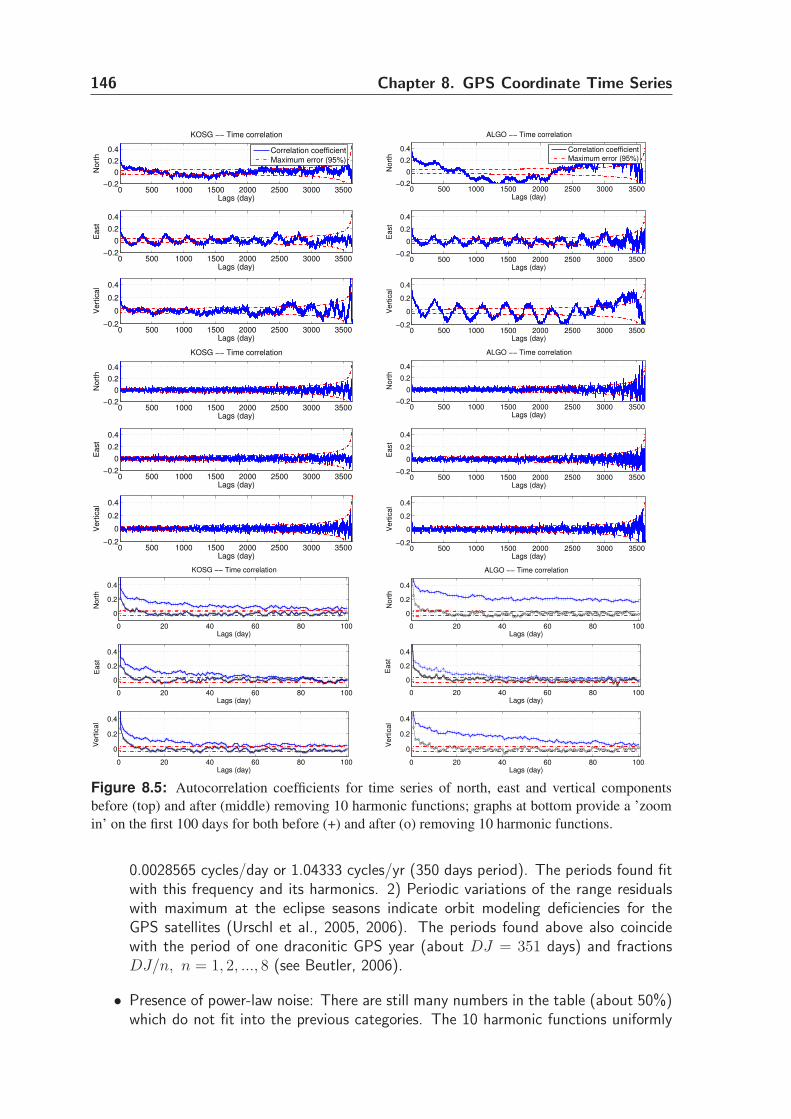
146 Chapter 8. GPS Coordinate Time Series
0 500 1000 1500 2000 2500 3000 3500−0.2
0
0.2
0.4
Nort
h
Lags (day)
KOSG −− Time correlation
0 500 1000 1500 2000 2500 3000 3500−0.2
0
0.2
0.4
East
Lags (day)
0 500 1000 1500 2000 2500 3000 3500−0.2
0
0.2
0.4
Vert
ical
Lags (day)
Correlation coefficient
Maximum error (95%)
0 500 1000 1500 2000 2500 3000 3500−0.2
0
0.2
0.4
No
rth
Lags (day)
ALGO −− Time correlation
0 500 1000 1500 2000 2500 3000 3500−0.2
0
0.2
0.4
Ea
st
Lags (day)
0 500 1000 1500 2000 2500 3000 3500−0.2
0
0.2
0.4
Ve
rtic
al
Lags (day)
Correlation coefficient
Maximum error (95%)
0 500 1000 1500 2000 2500 3000 3500−0.2
0
0.2
0.4
Nort
h
Lags (day)
KOSG −− Time correlation
0 500 1000 1500 2000 2500 3000 3500−0.2
0
0.2
0.4
East
Lags (day)
0 500 1000 1500 2000 2500 3000 3500−0.2
0
0.2
0.4
Vert
ical
Lags (day)
0 500 1000 1500 2000 2500 3000 3500−0.2
0
0.2
0.4
No
rth
Lags (day)
ALGO −− Time correlation
0 500 1000 1500 2000 2500 3000 3500−0.2
0
0.2
0.4
Ea
st
Lags (day)
0 500 1000 1500 2000 2500 3000 3500−0.2
0
0.2
0.4
Ve
rtic
al
Lags (day)
0 20 40 60 80 100
0
0.2
0.4
No
rth
Lags (day)
KOSG −− Time correlation
0 20 40 60 80 100
0
0.2
0.4
Ea
st
Lags (day)
0 20 40 60 80 100
0
0.2
0.4
Ve
rtic
al
Lags (day)
0 20 40 60 80 100
0
0.2
0.4
Nort
h
Lags (day)
ALGO −− Time correlation
0 20 40 60 80 100
0
0.2
0.4
East
Lags (day)
0 20 40 60 80 100
0
0.2
0.4
Vert
ical
Lags (day)
Figure 8.5: Autocorrelation coefficients for time series of north, east and vertical components
before (top) and after (middle) removing 10 harmonic functions; graphs at bottom provide a ’zoom
in’ on the first 100 days for both before (+) and after (o) removing 10 harmonic functions.
0.0028565 cycles/day or 1.04333 cycles/yr (350 days period). The periods found fitwith this frequency and its harmonics. 2) Periodic variations of the range residualswith maximum at the eclipse seasons indicate orbit modeling deficiencies for theGPS satellites (Urschl et al., 2005, 2006). The periods found above also coincidewith the period of one draconitic GPS year (about DJ = 351 days) and fractionsDJ/n, n = 1, 2, ..., 8 (see Beutler, 2006).
• Presence of power-law noise: There are still many numbers in the table (about 50%)which do not fit into the previous categories. The 10 harmonic functions uniformly
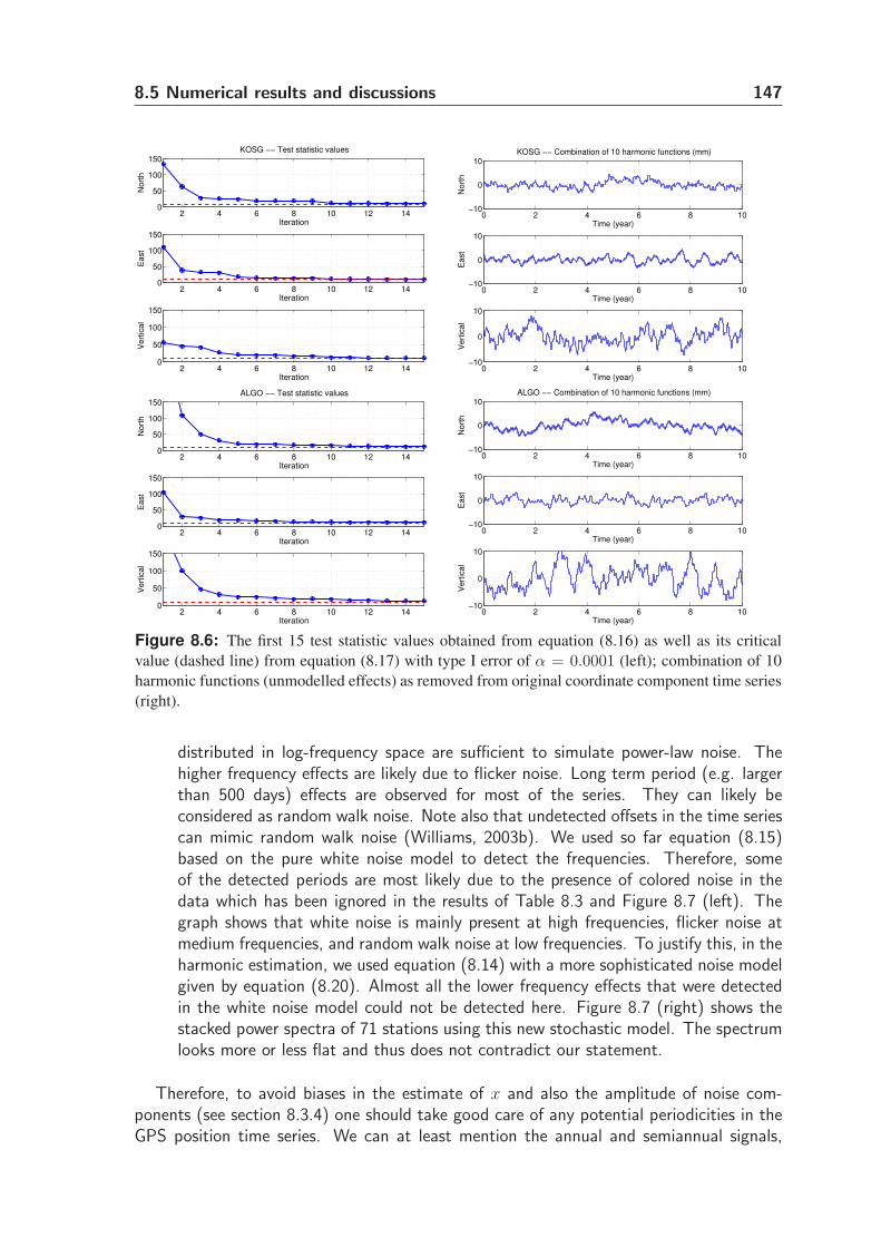
8.5 Numerical results and discussions 147
2 4 6 8 10 12 140
50
100
150
No
rth
Iteration
KOSG −− Test statistic values
2 4 6 8 10 12 140
50
100
150
Ea
st
Iteration
2 4 6 8 10 12 140
50
100
150
Ve
rtic
al
Iteration
0 2 4 6 8 10−10
0
10
Time (year)
No
rth
KOSG −− Combination of 10 harmonic functions (mm)
0 2 4 6 8 10−10
0
10
Time (year)
Ea
st
0 2 4 6 8 10−10
0
10
Time (year)
Ve
rtic
al
2 4 6 8 10 12 140
50
100
150
No
rth
Iteration
ALGO −− Test statistic values
2 4 6 8 10 12 140
50
100
150
Ea
st
Iteration
2 4 6 8 10 12 140
50
100
150
Ve
rtic
al
Iteration
0 2 4 6 8 10−10
0
10
Time (year)N
ort
h
ALGO −− Combination of 10 harmonic functions (mm)
0 2 4 6 8 10−10
0
10
Time (year)
Ea
st
0 2 4 6 8 10−10
0
10
Time (year)
Ve
rtic
al
Figure 8.6: The first 15 test statistic values obtained from equation (8.16) as well as its critical
value (dashed line) from equation (8.17) with type I error of α = 0.0001 (left); combination of 10
harmonic functions (unmodelled effects) as removed from original coordinate component time series
(right).
distributed in log-frequency space are sufficient to simulate power-law noise. Thehigher frequency effects are likely due to flicker noise. Long term period (e.g. largerthan 500 days) effects are observed for most of the series. They can likely beconsidered as random walk noise. Note also that undetected offsets in the time seriescan mimic random walk noise (Williams, 2003b). We used so far equation (8.15)based on the pure white noise model to detect the frequencies. Therefore, someof the detected periods are most likely due to the presence of colored noise in thedata which has been ignored in the results of Table 8.3 and Figure 8.7 (left). Thegraph shows that white noise is mainly present at high frequencies, flicker noise atmedium frequencies, and random walk noise at low frequencies. To justify this, in theharmonic estimation, we used equation (8.14) with a more sophisticated noise modelgiven by equation (8.20). Almost all the lower frequency effects that were detectedin the white noise model could not be detected here. Figure 8.7 (right) shows thestacked power spectra of 71 stations using this new stochastic model. The spectrumlooks more or less flat and thus does not contradict our statement.
Therefore, to avoid biases in the estimate of x and also the amplitude of noise com-ponents (see section 8.3.4) one should take good care of any potential periodicities in theGPS position time series. We can at least mention the annual and semiannual signals,
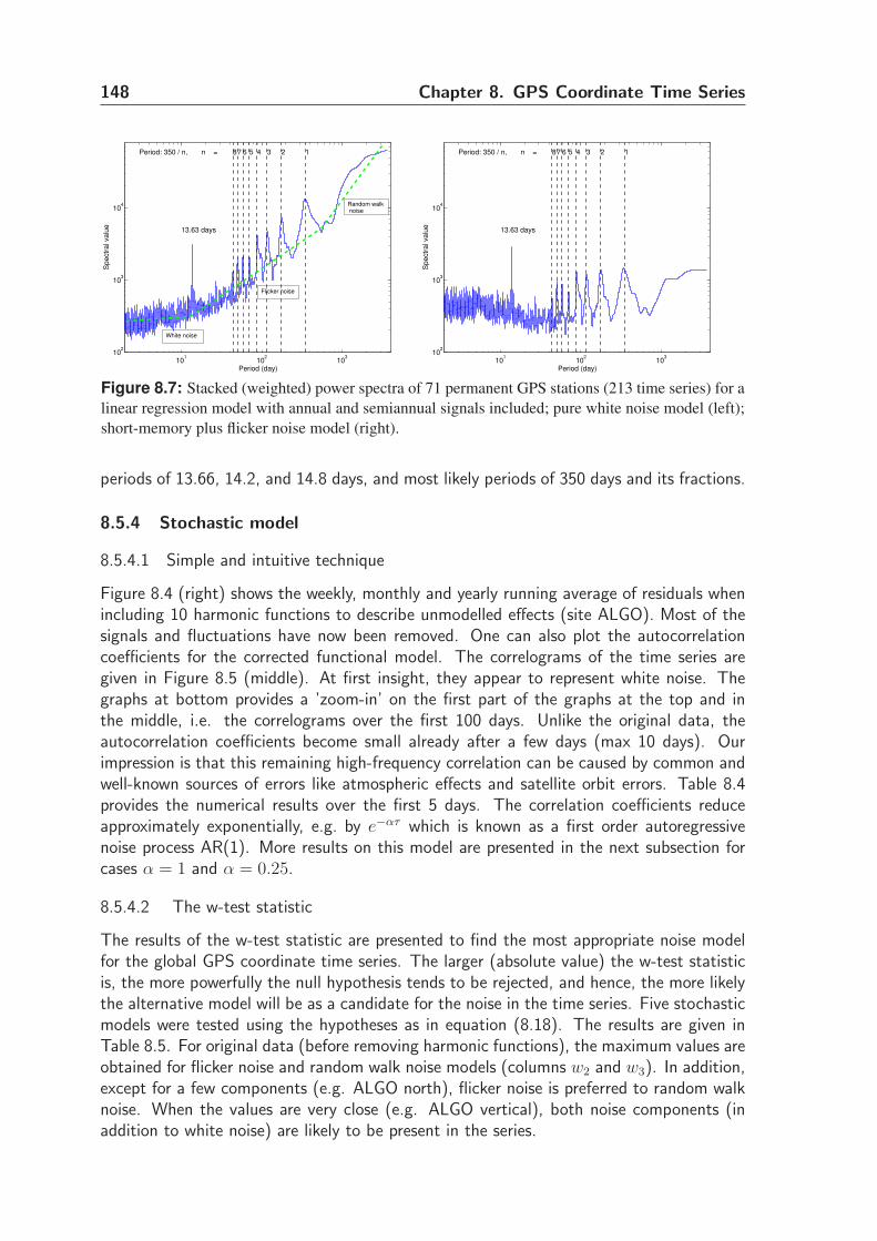
148 Chapter 8. GPS Coordinate Time Series
101
102
103
102
103
104
Period (day)
Sp
ectr
al va
lue
87 6 5 4 3 2 1Period: 350 / n, n =
13.63 days
White noise
Flicker noise
Random walk noise
101
102
103
102
103
104
87 6 5 4 3 2 1Period: 350 / n, n =
13.63 days
Period (day)
Sp
ectr
al va
lue
Figure 8.7: Stacked (weighted) power spectra of 71 permanent GPS stations (213 time series) for a
linear regression model with annual and semiannual signals included; pure white noise model (left);
short-memory plus flicker noise model (right).
periods of 13.66, 14.2, and 14.8 days, and most likely periods of 350 days and its fractions.
8.5.4 Stochastic model
8.5.4.1 Simple and intuitive technique
Figure 8.4 (right) shows the weekly, monthly and yearly running average of residuals whenincluding 10 harmonic functions to describe unmodelled effects (site ALGO). Most of thesignals and fluctuations have now been removed. One can also plot the autocorrelationcoefficients for the corrected functional model. The correlograms of the time series aregiven in Figure 8.5 (middle). At first insight, they appear to represent white noise. Thegraphs at bottom provides a ’zoom-in’ on the first part of the graphs at the top and inthe middle, i.e. the correlograms over the first 100 days. Unlike the original data, theautocorrelation coefficients become small already after a few days (max 10 days). Ourimpression is that this remaining high-frequency correlation can be caused by common andwell-known sources of errors like atmospheric effects and satellite orbit errors. Table 8.4provides the numerical results over the first 5 days. The correlation coefficients reduceapproximately exponentially, e.g. by e−ατ which is known as a first order autoregressivenoise process AR(1). More results on this model are presented in the next subsection forcases α = 1 and α = 0.25.
8.5.4.2 The w-test statistic
The results of the w-test statistic are presented to find the most appropriate noise modelfor the global GPS coordinate time series. The larger (absolute value) the w-test statisticis, the more powerfully the null hypothesis tends to be rejected, and hence, the more likelythe alternative model will be as a candidate for the noise in the time series. Five stochasticmodels were tested using the hypotheses as in equation (8.18). The results are given inTable 8.5. For original data (before removing harmonic functions), the maximum values areobtained for flicker noise and random walk noise models (columns w2 and w3). In addition,except for a few components (e.g. ALGO north), flicker noise is preferred to random walknoise. When the values are very close (e.g. ALGO vertical), both noise components (inaddition to white noise) are likely to be present in the series.
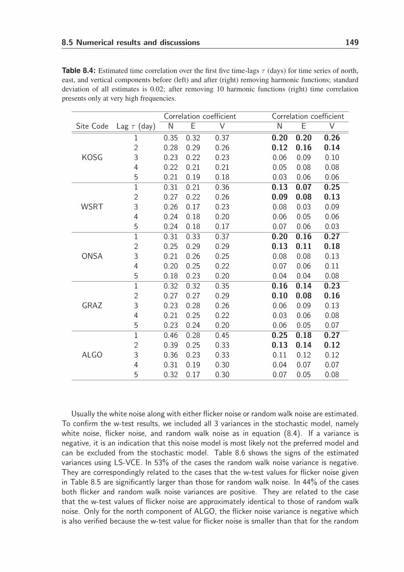
8.5 Numerical results and discussions 149
Table 8.4: Estimated time correlation over the first five time-lags τ (days) for time series of north,
east, and vertical components before (left) and after (right) removing harmonic functions; standard
deviation of all estimates is 0.02; after removing 10 harmonic functions (right) time correlation
presents only at very high frequencies.
Correlation coefficient Correlation coefficientSite Code Lag τ (day) N E V N E V
1 0.35 0.32 0.37 0.20 0.20 0.262 0.28 0.29 0.26 0.12 0.16 0.14
KOSG 3 0.23 0.22 0.23 0.06 0.09 0.104 0.22 0.21 0.21 0.05 0.08 0.085 0.21 0.19 0.18 0.03 0.06 0.061 0.31 0.21 0.36 0.13 0.07 0.252 0.27 0.22 0.26 0.09 0.08 0.13
WSRT 3 0.26 0.17 0.23 0.08 0.03 0.094 0.24 0.18 0.20 0.06 0.05 0.065 0.24 0.18 0.17 0.07 0.06 0.031 0.31 0.33 0.37 0.20 0.16 0.272 0.25 0.29 0.29 0.13 0.11 0.18
ONSA 3 0.21 0.26 0.25 0.08 0.08 0.134 0.20 0.25 0.22 0.07 0.06 0.115 0.18 0.23 0.20 0.04 0.04 0.081 0.32 0.32 0.35 0.16 0.14 0.232 0.27 0.27 0.29 0.10 0.08 0.16
GRAZ 3 0.23 0.28 0.26 0.06 0.09 0.134 0.21 0.25 0.22 0.03 0.06 0.085 0.23 0.24 0.20 0.06 0.05 0.071 0.46 0.28 0.45 0.25 0.18 0.272 0.39 0.25 0.33 0.13 0.14 0.12
ALGO 3 0.36 0.23 0.33 0.11 0.12 0.124 0.31 0.19 0.30 0.04 0.07 0.075 0.32 0.17 0.30 0.07 0.05 0.08
Usually the white noise along with either flicker noise or random walk noise are estimated.To confirm the w-test results, we included all 3 variances in the stochastic model, namelywhite noise, flicker noise, and random walk noise as in equation (8.4). If a variance isnegative, it is an indication that this noise model is most likely not the preferred model andcan be excluded from the stochastic model. Table 8.6 shows the signs of the estimatedvariances using LS-VCE. In 53% of the cases the random walk noise variance is negative.They are correspondingly related to the cases that the w-test values for flicker noise givenin Table 8.5 are significantly larger than those for random walk noise. In 44% of the casesboth flicker and random walk noise variances are positive. They are related to the casethat the w-test values of flicker noise are approximately identical to those of random walknoise. Only for the north component of ALGO, the flicker noise variance is negative whichis also verified because the w-test value for flicker noise is smaller than that for the random
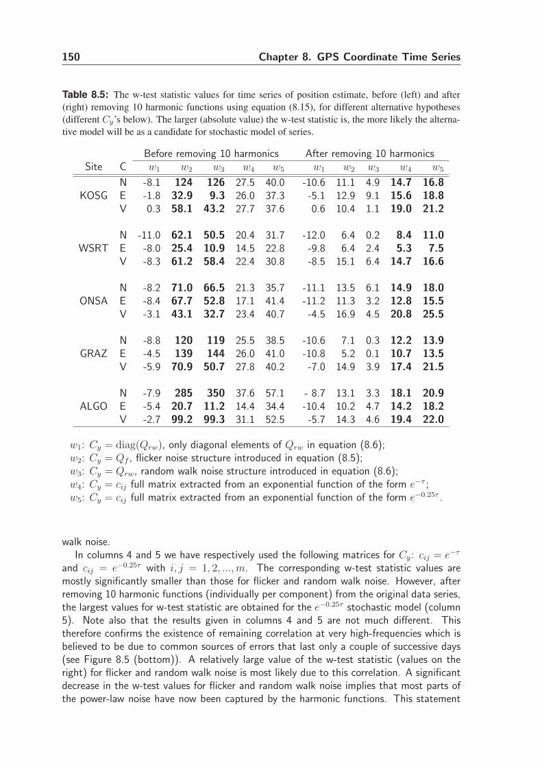
150 Chapter 8. GPS Coordinate Time Series
Table 8.5: The w-test statistic values for time series of position estimate, before (left) and after
(right) removing 10 harmonic functions using equation (8.15), for different alternative hypotheses
(different Cy’s below). The larger (absolute value) the w-test statistic is, the more likely the alterna-
tive model will be as a candidate for stochastic model of series.
Before removing 10 harmonics After removing 10 harmonicsSite C w1 w2 w3 w4 w5 w1 w2 w3 w4 w5
N -8.1 124 126 27.5 40.0 -10.6 11.1 4.9 14.7 16.8KOSG E -1.8 32.9 9.3 26.0 37.3 -5.1 12.9 9.1 15.6 18.8
V 0.3 58.1 43.2 27.7 37.6 0.6 10.4 1.1 19.0 21.2
N -11.0 62.1 50.5 20.4 31.7 -12.0 6.4 0.2 8.4 11.0WSRT E -8.0 25.4 10.9 14.5 22.8 -9.8 6.4 2.4 5.3 7.5
V -8.3 61.2 58.4 22.4 30.8 -8.5 15.1 6.4 14.7 16.6
N -8.2 71.0 66.5 21.3 35.7 -11.1 13.5 6.1 14.9 18.0ONSA E -8.4 67.7 52.8 17.1 41.4 -11.2 11.3 3.2 12.8 15.5
V -3.1 43.1 32.7 23.4 40.7 -4.5 16.9 4.5 20.8 25.5
N -8.8 120 119 25.5 38.5 -10.6 7.1 0.3 12.2 13.9GRAZ E -4.5 139 144 26.0 41.0 -10.8 5.2 0.1 10.7 13.5
V -5.9 70.9 50.7 27.8 40.2 -7.0 14.9 3.9 17.4 21.5
N -7.9 285 350 37.6 57.1 - 8.7 13.1 3.3 18.1 20.9ALGO E -5.4 20.7 11.2 14.4 34.4 -10.4 10.2 4.7 14.2 18.2
V -2.7 99.2 99.3 31.1 52.5 -5.7 14.3 4.6 19.4 22.0
w1: Cy = diag(Qrw), only diagonal elements of Qrw in equation (8.6);w2: Cy = Qf , flicker noise structure introduced in equation (8.5);w3: Cy = Qrw, random walk noise structure introduced in equation (8.6);w4: Cy = cij full matrix extracted from an exponential function of the form e−τ ;w5: Cy = cij full matrix extracted from an exponential function of the form e−0.25τ .
walk noise.In columns 4 and 5 we have respectively used the following matrices for Cy: cij = e−τ
and cij = e−0.25τ with i, j = 1, 2, ...,m. The corresponding w-test statistic values aremostly significantly smaller than those for flicker and random walk noise. However, afterremoving 10 harmonic functions (individually per component) from the original data series,the largest values for w-test statistic are obtained for the e−0.25τ stochastic model (column5). Note also that the results given in columns 4 and 5 are not much different. Thistherefore confirms the existence of remaining correlation at very high-frequencies which isbelieved to be due to common sources of errors that last only a couple of successive days(see Figure 8.5 (bottom)). A relatively large value of the w-test statistic (values on theright) for flicker and random walk noise is most likely due to this correlation. A significantdecrease in the w-test values for flicker and random walk noise implies that most parts ofthe power-law noise have now been captured by the harmonic functions. This statement
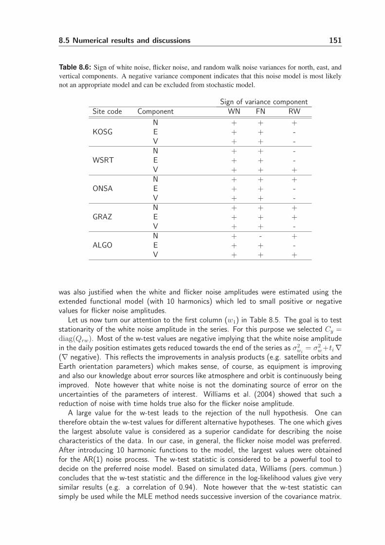
8.5 Numerical results and discussions 151
Table 8.6: Sign of white noise, flicker noise, and random walk noise variances for north, east, and
vertical components. A negative variance component indicates that this noise model is most likely
not an appropriate model and can be excluded from stochastic model.
Sign of variance componentSite code Component WN FN RW
N + + +KOSG E + + -
V + + -N + + -
WSRT E + + -V + + +N + + +
ONSA E + + -V + + -N + + +
GRAZ E + + +V + + -N + - +
ALGO E + + -V + + +
was also justified when the white and flicker noise amplitudes were estimated using theextended functional model (with 10 harmonics) which led to small positive or negativevalues for flicker noise amplitudes.
Let us now turn our attention to the first column (w1) in Table 8.5. The goal is to teststationarity of the white noise amplitude in the series. For this purpose we selected Cy =diag(Qrw). Most of the w-test values are negative implying that the white noise amplitudein the daily position estimates gets reduced towards the end of the series as σ2
wi= σ2
w +ti∇(∇ negative). This reflects the improvements in analysis products (e.g. satellite orbits andEarth orientation parameters) which makes sense, of course, as equipment is improvingand also our knowledge about error sources like atmosphere and orbit is continuously beingimproved. Note however that white noise is not the dominating source of error on theuncertainties of the parameters of interest. Williams et al. (2004) showed that such areduction of noise with time holds true also for the flicker noise amplitude.
A large value for the w-test leads to the rejection of the null hypothesis. One cantherefore obtain the w-test values for different alternative hypotheses. The one which givesthe largest absolute value is considered as a superior candidate for describing the noisecharacteristics of the data. In our case, in general, the flicker noise model was preferred.After introducing 10 harmonic functions to the model, the largest values were obtainedfor the AR(1) noise process. The w-test statistic is considered to be a powerful tool todecide on the preferred noise model. Based on simulated data, Williams (pers. commun.)concludes that the w-test statistic and the difference in the log-likelihood values give verysimilar results (e.g. a correlation of 0.94). Note however that the w-test statistic cansimply be used while the MLE method needs successive inversion of the covariance matrix.
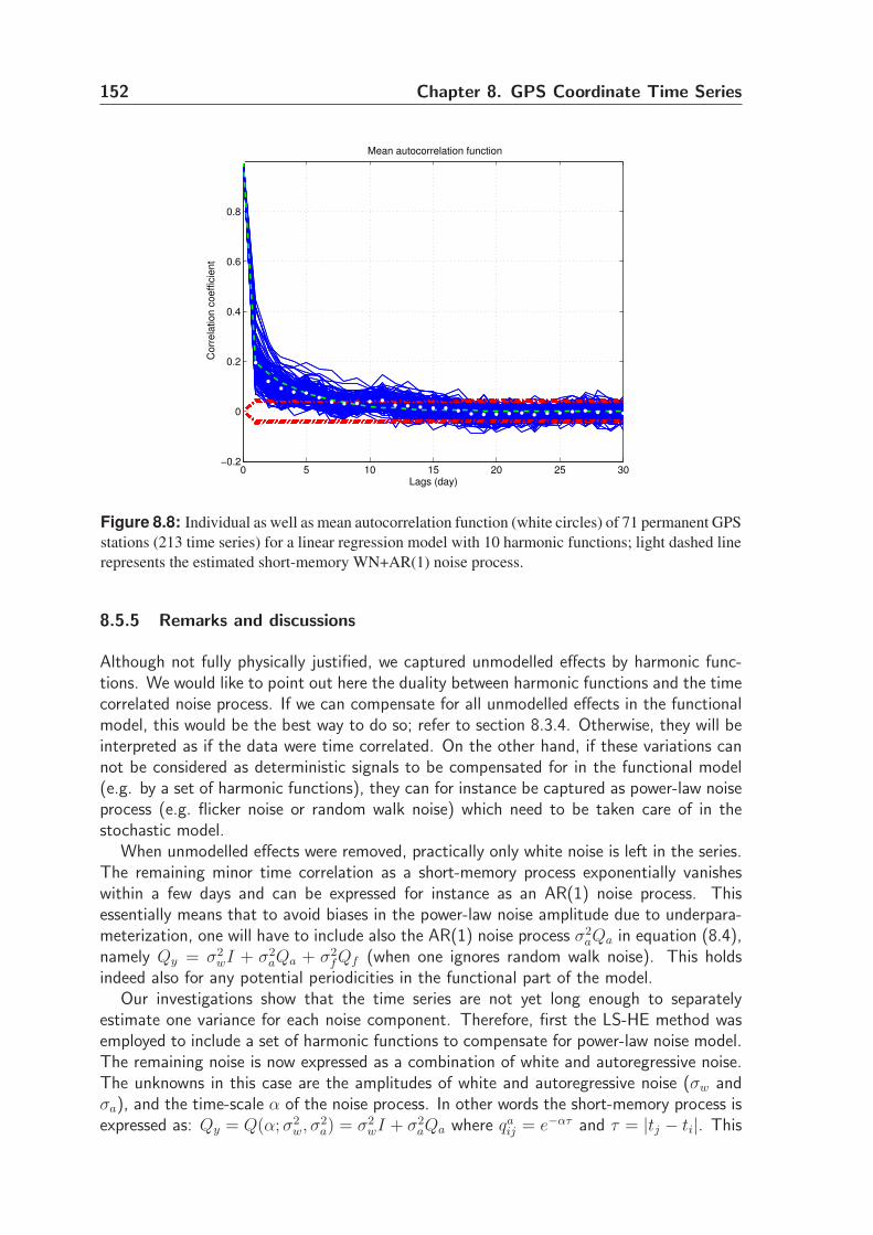
152 Chapter 8. GPS Coordinate Time Series
0 5 10 15 20 25 30−0.2
0
0.2
0.4
0.6
0.8C
orr
ela
tion c
oeffic
ient
Lags (day)
Mean autocorrelation function
Figure 8.8: Individual as well as mean autocorrelation function (white circles) of 71 permanent GPS
stations (213 time series) for a linear regression model with 10 harmonic functions; light dashed line
represents the estimated short-memory WN+AR(1) noise process.
8.5.5 Remarks and discussions
Although not fully physically justified, we captured unmodelled effects by harmonic func-tions. We would like to point out here the duality between harmonic functions and the timecorrelated noise process. If we can compensate for all unmodelled effects in the functionalmodel, this would be the best way to do so; refer to section 8.3.4. Otherwise, they will beinterpreted as if the data were time correlated. On the other hand, if these variations cannot be considered as deterministic signals to be compensated for in the functional model(e.g. by a set of harmonic functions), they can for instance be captured as power-law noiseprocess (e.g. flicker noise or random walk noise) which need to be taken care of in thestochastic model.
When unmodelled effects were removed, practically only white noise is left in the series.The remaining minor time correlation as a short-memory process exponentially vanisheswithin a few days and can be expressed for instance as an AR(1) noise process. Thisessentially means that to avoid biases in the power-law noise amplitude due to underpara-meterization, one will have to include also the AR(1) noise process σ2
aQa in equation (8.4),namely Qy = σ2
wI + σ2aQa + σ2
fQf (when one ignores random walk noise). This holdsindeed also for any potential periodicities in the functional part of the model.
Our investigations show that the time series are not yet long enough to separatelyestimate one variance for each noise component. Therefore, first the LS-HE method wasemployed to include a set of harmonic functions to compensate for power-law noise model.The remaining noise is now expressed as a combination of white and autoregressive noise.The unknowns in this case are the amplitudes of white and autoregressive noise (σw andσa), and the time-scale α of the noise process. In other words the short-memory process isexpressed as: Qy = Q(α; σ2
w, σ2a) = σ2
wI + σ2aQa where qa
ij = e−ατ and τ = |tj − ti|. This
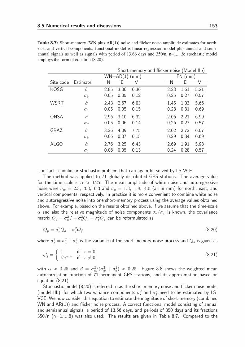
8.5 Numerical results and discussions 153
Table 8.7: Short-memory (WN plus AR(1)) noise and flicker noise amplitude estimates for north,
east, and vertical components; functional model is linear regression model plus annual and semi-
annual signals as well as signals with period of 13.66 days and 350/n, n=1,...,8; stochastic model
employs the form of equation (8.20).
Short-memory and flicker noise (Model IIb)WN+AR(1) (mm) FN (mm)
Site code Estimate N E V N E V
KOSG σ 2.85 3.06 6.36 2.23 1.61 5.21σσ 0.05 0.05 0.12 0.25 0.27 0.57
WSRT σ 2.43 2.67 6.03 1.45 1.03 5.66σσ 0.05 0.05 0.15 0.28 0.31 0.69
ONSA σ 2.96 3.10 6.32 2.06 2.21 6.99σσ 0.05 0.06 0.14 0.26 0.27 0.57
GRAZ σ 3.26 4.09 7.75 2.02 2.72 6.07σσ 0.06 0.07 0.15 0.29 0.34 0.69
ALGO σ 2.76 3.25 6.43 2.69 1.91 5.98σσ 0.06 0.05 0.13 0.24 0.28 0.57
is in fact a nonlinear stochastic problem that can again be solved by LS-VCE.The method was applied to 71 globally distributed GPS stations. The average value
for the time-scale is α ≈ 0.25. The mean amplitude of white noise and autoregressivenoise were σw = 2.3, 3.3, 6.3 and σa = 1.3, 1.8, 4.0 (all in mm) for north, east, andvertical components, respectively. In practice it is more convenient to combine white noiseand autoregressive noise into one short-memory process using the average values obtainedabove. For example, based on the results obtained above, if we assume that the time-scaleα and also the relative magnitude of noise components σa/σw is known, the covariancematrix Qy = σ2
wI + σ2aQa + σ2
fQf can be reformulated as
Qy = σ2sQs + σ2
fQf (8.20)
where σ2s = σ2
a + σ2w is the variance of the short-memory noise process and Qs is given as
qsij =
{1 if τ = 0βe−ατ if τ 6= 0
(8.21)
with α ≈ 0.25 and β = σ2a/(σ
2w + σ2
a) ≈ 0.25. Figure 8.8 shows the weighted meanautocorrelation function of 71 permanent GPS stations, and its approximation based onequation (8.21).
Stochastic model (8.20) is referred to as the short-memory noise and flicker noise model(model IIb), for which two variance components σ2
s and σ2f need to be estimated by LS-
VCE. We now consider this equation to estimate the magnitude of short-memory (combinedWN and AR(1)) and flicker noise process. A correct functional model consisting of annualand semiannual signals, a period of 13.66 days, and periods of 350 days and its fractions350/n (n=1,...,8) was also used. The results are given in Table 8.7. Compared to the
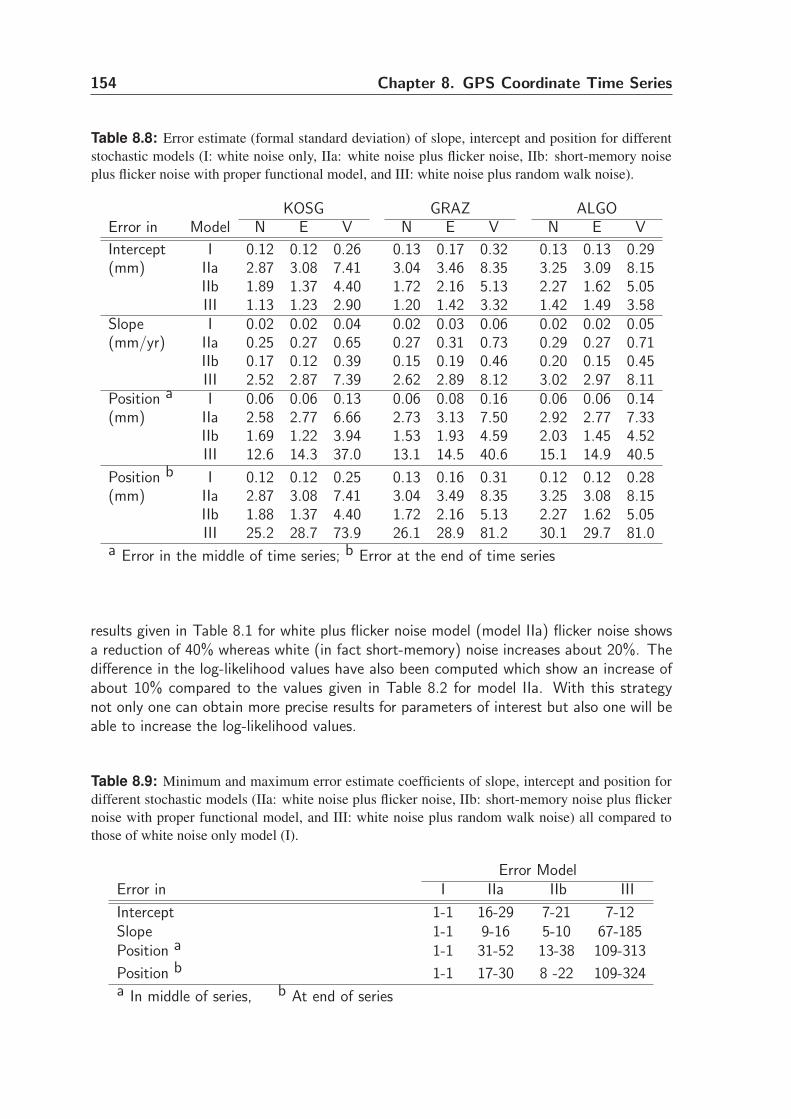
154 Chapter 8. GPS Coordinate Time Series
Table 8.8: Error estimate (formal standard deviation) of slope, intercept and position for different
stochastic models (I: white noise only, IIa: white noise plus flicker noise, IIb: short-memory noise
plus flicker noise with proper functional model, and III: white noise plus random walk noise).
KOSG GRAZ ALGOError in Model N E V N E V N E V
Intercept I 0.12 0.12 0.26 0.13 0.17 0.32 0.13 0.13 0.29(mm) IIa 2.87 3.08 7.41 3.04 3.46 8.35 3.25 3.09 8.15
IIb 1.89 1.37 4.40 1.72 2.16 5.13 2.27 1.62 5.05III 1.13 1.23 2.90 1.20 1.42 3.32 1.42 1.49 3.58
Slope I 0.02 0.02 0.04 0.02 0.03 0.06 0.02 0.02 0.05(mm/yr) IIa 0.25 0.27 0.65 0.27 0.31 0.73 0.29 0.27 0.71
IIb 0.17 0.12 0.39 0.15 0.19 0.46 0.20 0.15 0.45III 2.52 2.87 7.39 2.62 2.89 8.12 3.02 2.97 8.11
Position a I 0.06 0.06 0.13 0.06 0.08 0.16 0.06 0.06 0.14(mm) IIa 2.58 2.77 6.66 2.73 3.13 7.50 2.92 2.77 7.33
IIb 1.69 1.22 3.94 1.53 1.93 4.59 2.03 1.45 4.52III 12.6 14.3 37.0 13.1 14.5 40.6 15.1 14.9 40.5
Position b I 0.12 0.12 0.25 0.13 0.16 0.31 0.12 0.12 0.28(mm) IIa 2.87 3.08 7.41 3.04 3.49 8.35 3.25 3.08 8.15
IIb 1.88 1.37 4.40 1.72 2.16 5.13 2.27 1.62 5.05III 25.2 28.7 73.9 26.1 28.9 81.2 30.1 29.7 81.0
a Error in the middle of time series; b Error at the end of time series
results given in Table 8.1 for white plus flicker noise model (model IIa) flicker noise showsa reduction of 40% whereas white (in fact short-memory) noise increases about 20%. Thedifference in the log-likelihood values have also been computed which show an increase ofabout 10% compared to the values given in Table 8.2 for model IIa. With this strategynot only one can obtain more precise results for parameters of interest but also one will beable to increase the log-likelihood values.
Table 8.9: Minimum and maximum error estimate coefficients of slope, intercept and position for
different stochastic models (IIa: white noise plus flicker noise, IIb: short-memory noise plus flicker
noise with proper functional model, and III: white noise plus random walk noise) all compared to
those of white noise only model (I).
Error ModelError in I IIa IIb III
Intercept 1-1 16-29 7-21 7-12Slope 1-1 9-16 5-10 67-185Position a 1-1 31-52 13-38 109-313
Position b 1-1 17-30 8 -22 109-324a In middle of series, b At end of series
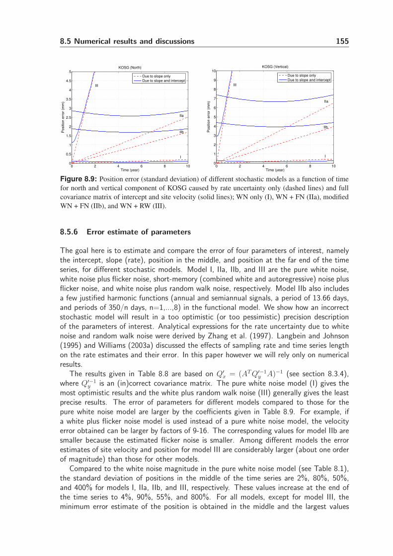
8.5 Numerical results and discussions 155
0 2 4 6 8 100
0.5
1
1.5
2
2.5
3
3.5
4
4.5
5
Time (year)
Po
sitio
n e
rro
r (m
m)
KOSG (North)
III
IIb
IIa
I
Due to slope only
Due to slope and intercept
0 2 4 6 8 100
1
2
3
4
5
6
7
8
9
10
Time (year)
Positio
n e
rror
(mm
)
KOSG (Vertical)
III
IIb
IIa
I
Due to slope only
Due to slope and intercept
Figure 8.9: Position error (standard deviation) of different stochastic models as a function of time
for north and vertical component of KOSG caused by rate uncertainty only (dashed lines) and full
covariance matrix of intercept and site velocity (solid lines); WN only (I), WN + FN (IIa), modified
WN + FN (IIb), and WN + RW (III).
8.5.6 Error estimate of parameters
The goal here is to estimate and compare the error of four parameters of interest, namelythe intercept, slope (rate), position in the middle, and position at the far end of the timeseries, for different stochastic models. Model I, IIa, IIb, and III are the pure white noise,white noise plus flicker noise, short-memory (combined white and autoregressive) noise plusflicker noise, and white noise plus random walk noise, respectively. Model IIb also includesa few justified harmonic functions (annual and semiannual signals, a period of 13.66 days,and periods of 350/n days, n=1,...,8) in the functional model. We show how an incorrectstochastic model will result in a too optimistic (or too pessimistic) precision descriptionof the parameters of interest. Analytical expressions for the rate uncertainty due to whitenoise and random walk noise were derived by Zhang et al. (1997). Langbein and Johnson(1995) and Williams (2003a) discussed the effects of sampling rate and time series lengthon the rate estimates and their error. In this paper however we will rely only on numericalresults.
The results given in Table 8.8 are based on Q′x = (AT Q′−1
y A)−1 (see section 8.3.4),where Q′−1
y is an (in)correct covariance matrix. The pure white noise model (I) gives themost optimistic results and the white plus random walk noise (III) generally gives the leastprecise results. The error of parameters for different models compared to those for thepure white noise model are larger by the coefficients given in Table 8.9. For example, ifa white plus flicker noise model is used instead of a pure white noise model, the velocityerror obtained can be larger by factors of 9-16. The corresponding values for model IIb aresmaller because the estimated flicker noise is smaller. Among different models the errorestimates of site velocity and position for model III are considerably larger (about one orderof magnitude) than those for other models.
Compared to the white noise magnitude in the pure white noise model (see Table 8.1),the standard deviation of positions in the middle of the time series are 2%, 80%, 50%,and 400% for models I, IIa, IIb, and III, respectively. These values increase at the end ofthe time series to 4%, 90%, 55%, and 800%. For all models, except for model III, theminimum error estimate of the position is obtained in the middle and the largest values
156 Chapter 8. GPS Coordinate Time Series
are given at both ends of the series. The results of model I are too optimistic. The errorcontribution of the intercept and the slope on the position seems to be the same (2% inthe middle and 4% at both ends). The results obtained from models IIa and IIb appearto be more realistic. In Model IIa the slope error has only a contribution of 10% on theposition error estimate (compare 80% in the middle vs 90% at both ends). The error inthe intercept plays the main role. This holds also for model IIb. When compared withmodel IIa, the results with model IIb get improved by a factor of 1.6. The behavior of thewhite noise plus random walk noise is somehow different. The results are too pessimisticand the error in the slope plays the main role.
In geophysical literature, the site velocity uncertainty is usually of interest and notdirectly the position error. However, in some geodesy applications (e.g. realization ofITRF) the final goal of the site velocity is in fact the position and its uncertainty. Thismeans that so far we have ignored the uncertainty of the intercept. In models IIa and IIbthe intercept plays the main role of error. Figure 8.9 shows the effect of site velocity onlyand site velocity plus intercept on the position error for different stochastic models. Wheninterested in position error and relying only on the site velocity error, it seems that modelsIIa and IIb are more appropriate for long-term accuracy but give optimistic results overshort periods. On the other hand, model III is likely suitable for short-term accuracy butyields pessimistic results over long periods (see Figure 8.9).
8.6 Summary and conclusions
We assessed the noise characteristics in global time series of daily position estimates by LS-VCE. The method is easily understood, generally applicable and very flexible. The LS-VCEestimators are unbiased and of minimum variance. This method provides the precision ofthe (co)variance estimators. Based on the results given, the following conclusions can bedrawn:
The w-test statistic is a powerful tool to recognize the data noise characteristics in orderto construct an appropriate stochastic model. Using the w-test a combination of short-memory (white plus autoregressive) noise and flicker noise was in general found to bestdescribe the noise characteristics of the position components; we hardly observed that thestrict white plus random walk was the preferred noise model. These results have also beenverified using correlograms of the time series, the frequencies of the harmonic functions,and the signs of the estimated flicker and random walk noise variance components.
The least-squares harmonic estimation method was used to find and consequently re-move a set of harmonic functions from the data. These harmonic functions capturedunmodelled effects. The results confirm the presence of annual and semiannual signals inthe series. We could also observe other periodic effects; for example a period of 13.66,14.2, and 14.8 days. We observed also significant periodic patterns with periods of 350days and its fractions 350/n, n=1,2,...,8 which is likely due to the aliased multipath ef-fects in permanent stations. When such variations have underlying physical phenomena(or modeling error), their effects can be considered as systematic periodic signals. It maynot be appropriate to capture their effects by a power-law noise process in the stochasticmodel. They may mistakenly mimic flicker or random walk noise if we neglect them inthe functional model. Therefore, neglecting such effects, which may be best described bya deterministic model rather than a power-law noise model, can seriously affect the error
8.6 Summary and conclusions 157
estimate of the site velocity and the position.There are also some effects in the series that are not of periodic nature. They can most
likely be expressed as power-law noise. We however employed the harmonic estimationmethod to find more frequencies in the series. A significant decrease in the w-test valuesfor power-law noise implies that most parts of this noise are captured by the harmonicfunctions. This led us to see a duality between the stochastic and functional model; whatis not captured in the functional model is captured in the stochastic model. When weinclude the harmonic functions, almost exclusively white noise remains in the data. Onlyat very high frequencies a significant time-correlation appeared to be present which can beexpressed as an exponential function (e.g. a first-order autoregressive noise process). Thisnoise can be caused by common sources of error like atmospheric effects as well as satelliteorbit errors that last over only a few successive days.
The overestimation of the power-law noise was due to the presence of the autoregressivenoise and also the justified hidden periodic effects in the series. This means that neitherthe white noise plus flicker noise model nor the white noise plus random walk noise modelis the preferred model. The best model includes in addition to power-law noise also othernoise models like autoregressive noise or as Langbein (2004) used the band-pass-filterednoise. Instead of strict white noise model a short-memory noise process was introducedwhich led to the reduction of the flicker noise magnitude.

Conclusions and Recommendations 99.1 Introduction
The least-squares method is one of the leading principles in the estimation of unknownparameters. In this thesis we introduced and used the least-squares variance componentestimation (LS-VCE) method. The research objective was focused on the theoretical aswell as practical aspects of LS-VCE for which two different applications of LS-VCE to realdata were considered.
To see the analogy with the functional model, we started by reviewing the standard least-squares theory with a linear model in chapter 2. This chapter consists of the estimationpart which includes the weighted least-squares estimator, the minimum variance estimator(BLUE), and the maximum likelihood estimator (MLE), but also consists of the validationpart which includes the w-test, v-test, and overall model test. In chapter 3 we reviewedthe many different variance component estimation methods. We can at least mentionthe MINQUE, BIQUE, and MLE methods. The underlying assumptions of each methodwere discussed. The methods give identical estimators under the normality assumption.Chapters 4, 5, and 6 form the body of knowledge of our least-squares variance componentestimation and validation theory. Chapters 7 and 8 dealt with applications of LS-VCE toreal GPS data. In the next section we summarize the key points of our achievements andeventually provide recommendations for further research.
9.2 Summary
Since the LS-VCE method is undeservedly still one of the lesser known VCE-methods, inchapters 4 and 5, we emphasized that LS-VCE is a simple, flexible, and attractive method.The method is simple since it formulates the variance component estimation model in termsof a model of observation equations with the observable vector y
vh= vh(t tT −BT Q0B),
the design matrix Avh = [vh(BT Q1B), . . . , vh(BT QpB)], and the positive-definite weightmatrix Wvh. The unbiased least-squares estimator of the (co)variance component vectorfollows directly as
σ = (ATvhWvhAvh)
−1ATvhWvhyvh
= N−1l , (9.1)
where the p× p matrix N and the p-vector l are obtained from t, BT Q1B,...,BT QpB andWvh. The unbiasedness property follows directly from the weighted least-squares theoryand is independent of the (un)specified distribution of the observables either y or vh(t tT ).The method is flexible, since it works with a user-defined weight matrix Wvh. One hasthus the possibility to use different classes of weight matrices, one of which is given as
160 Chapter 9. Conclusions and Recommendations
Wvh = DT (Wt ⊗Wt)D with D the duplication matrix and Wt a positive-definite matrix.Another weight matrix class follows from the class of elliptically contoured distributions.
The LS-VCE method is also attractive, since it allows one to directly apply the existingbody of knowledge of least-squares theory. We addressed measures of inconsistencies in thestochastic model, the use of a-priori (co)variance component estimation, the estimabilityof variance components, robust estimation of variance components, non-negative variancecomponents, and nonlinear variance component estimation. The precision description of the(co)variance component estimator easily follows from application of the error propagationlaw to equation (9.1), as
Qσ = N−1MN−1 , (9.2)
with N = ATvhWvhAvh, M = AT
vhWvhQvhWvhAvh and Qvh the covariance matrix of yvh
.Being able to perform a rigorous precision analysis is important for many applications, suchas estimability analysis and significance testing.
In an analogous way to chapter 2 we described the weighted least-squares estimator,the minimum variance estimator, and the maximum likelihood estimator to VCE. To imple-ment the minimum variance estimators of (co)variance components, iterative step-by-stepprocedures were proposed; two equivalent formulation were given. The last part of chap-ter 4 was focused on inadmissible variance and covariance components. This can be thecase for instance when estimated variance components are negative. Some defects of theVCE model in which the (co)variance components are inestimable or poorly estimable werediscussed as well. This was achieved by using a few illustrative examples.
We applied hypothesis testing with the stochastic model, which is the subject of discus-sion in chapter 5. We presented the w-test, v-test, and overall model test for the stochasticmodel. The w-test statistic is used to see whether or not a certain noise component islikely to be present in the data set at hand, which consequently can be included in thestochastic model. Following the standard least-squares theory, this test statistic is given as
w =〈P⊥
Avhvh(Ct), P
⊥Avh
vh(t tT )〉‖P⊥
Avhvh(Ct)‖Q−1
vh
, (9.3)
where Ct is a cofactor matrix under the alternative hypothesis. Based on the normaldistribution of the original observables we determined the mean, variance, and distributionof the w-test statistic. Under the null hypothesis, the mean is zero and the variance isone. The distribution is a linear combination of mutually independent central chi-squaredistributions each with one degree of freedom.
An equivalent expression was given by introducing the v-test statistic. The goal is todecrease the number of (co)variance components of the stochastic model by testing thesignificance of the (co)variance components. If one (co)variance component is insignificant,that component can likely be excluded from the stochastic model. The overall model testwas also introduced to generally validate a proposed stochastic model.
In chapters 7 and 8 we applied LS-VCE to real data. The LS-VCE method was appliedto the GPS geometry-free observation model in chapter 7. This model is linear and canbe easily implemented in computer code. We started by formulating the functional andstochastic model of the GPS observables. Mainly, the variance component of differentobservation types, the satellite elevation dependence of GPS observables precision, and thecorrelation between different observation types were considered. We showed for instance
9.3 Conclusions 161
that the precision of the GPS observables depends, to a large extent, upon the elevationof satellites. Also, significant correlation between observation types was found. In orderto obtain the minimum variance estimators, and for a proper precision description of theestimates, such important issues should be taken into account in the covariance matrix ofthe GPS observables.
In chapter 8 we proposed a methodology to assess the noise characteristics in time seriesof daily position estimates for permanent GPS stations in a global reference frame. Wealso applied the statistical tests to find an appropriate stochastic model of GPS time series.Using the w-test statistic values, a combination of white noise and flicker noise turned outin general to best characterize the noise in all three position components. An interpretationfor the colored noise of the series was given. Unmodelled periodic effects in the data werecaptured by a set of harmonic functions for which we relied on the least-squares harmonicestimation (LS-HE) method and parameter significance testing developed in the sameframework as LS-VCE. Having included harmonic functions into the model, practically onlywhite noise was observed to remain in the data. Remaining time-correlation was presentonly at very high frequencies (spanning a few days only) which was best expressed as a firstorder autoregressive noise process. This noise can be caused by common and well-knownsources of error like unmodelled tropospheric and ionospheric effects as well as satelliteorbit errors. The results confirmed the presence of annual and semiannual signals in theseries. We observed also other significant periodic patterns in the series.
9.3 Conclusions
On the basis of the presented theory and the numerical results obtained with real data, thefollowing conclusions can be drawn:
Unification of methods The LS-VCE method is capable of unifying many of the existingVCE-methods. These methods can be easily recovered by making appropriate choices forthe weight matrix Wvh. From equation (9.1) one directly obtains the minimum variance(co)variance component estimator, if the weight matrix is chosen as Wvh = Q−1
vh . Thecovariance matrix Qvh and its inverse were worked out for the normal distributions. We alsomade some statements for a class of elliptically contoured distributions. Several importantdistributions are known to belong to this class, the multivariate normal distribution beingone such example. In case of the normal distribution, the REML and the BIQUE arerecovered. Without any distribution assumption, the MINQUE can also be recovered fromthe LS-VCE method by making a particular choice for the weight matrix, namely Wt = Q−1
t
in Wvh = DT (Wt ⊗Wt)D.
LS-VCE method LS-VCE is a powerful method for the estimation and validation of thestochastic model parameters. Since the method is based on the least-squares principle,we can directly apply the existing body of knowledge of least-squares theory to the VCEproblem. For example it allows one to easily obtain the covariance matrix of the estimators,and also measures of discrepancies such as the quadratic form of the residuals and the w-test statistics can readily be obtained. This can play an important role if one wants to applythe standard quality control theory to the stochastic model. The use of a-priori (co)variancecomponent information, robust estimation of variance components, non-negative variancecomponents, and nonlinear covariance functions can also be dealt with in LS-VCE. This
162 Chapter 9. Conclusions and Recommendations
method can thus be introduced as a standard method for estimation and validation of the(co)variance components of the stochastic model.
Estimability In order for the stochastic model to have a unique solution, the columnsof the design matrix Avh should be linearly independent. The necessary and sufficientcondition, for the stochastic model to have a unique solution, is thus linear independence ofthe cofactor matrices BT Q1B, ... , BT QpB. Therefore, linear independence of Q1, ... , Qp
is only a necessary condition, and not a sufficient one. One can apply the idea of thegeneralized inverses and the S-transformations to the rank-deficient system of equations inthe stochastic model. Estimability, admissibility, and ill-posedness of the stochastic modelare three key issues that need to be taken care of in practice. Modification of the variancecomponent model, choosing reasonably good a-priori values for (co)variance componentsand increasing the redundancy of the functional model, and thereby the redundancy of thestochastic model, cure usually such problems.
Distribution In this thesis we introduced hypotheses testing in the stochastic model. Thegoal is to come up with an appropriate stochastic model which includes the proper noisecomponents into the covariance matrix, for which we rely on the w-test and v-test statistic.In general, the distribution of the w-test and v-test statistic in the stochastic model is notnormal if the original observables are normally distributed. However, based on the centrallimit theorem, for some special cases, if the redundancy of the model is large enough,the distribution can be approximated by the standard normal distribution. Based on thesimulation of a few examples (not included in this thesis) we could draw the same conclusionfor different forms of the functional and stochastic model. To stay on the safe side, for therejection of the null hypothesis, one can also use the Chebyschev inequality which is alwaysindependent of the distribution. The Chebyschev inequality does not provide us with asharp confidence interval (usually gives an upper bound for a specified level of significanceα). However, there is no danger with using this if our testing results in the rejection ofthe null hypothesis. For example, lots of the large values of the w-test statistic given intable 8.5 can simply results in the rejection of the null hypothesis using the Chebyschevinequality. We could thereby conclude that the noise in GPS coordinate time series wasbest described by a combination of white noise, flicker noise, and autoregressive noise.
Geometry-free model It this thesis we considered the GPS geometry-free (double dif-ference) observation model to assess the stochastics of the GPS code and carrier phaseobservations. As expected, the variance of a GPS observable generally depends on the ele-vation of the satellite. Also, significant correlation can occur between different observationtypes, e.g. between the C1 and P2 codes. For high-precision positioning applications, toobtain best (minimum variance) estimators, it is necessary to use an appropriate covari-ance matrix for the observables, since W = Q−1
y . Using the GPS geometry free observationmodel, we could only assess the noise behavior of the GPS observables partially. Since thegeometry-based model is stronger than the geometry-free model, the use of this model ismore fruitful for the application of VCE to GPS observables (see next section).
Time series analysis To obtain a realistic precision description of the estimates for theunknown parameters in the functional model, a proper covariance matrix of the data isrequired. This means that if the covariance matrix is being estimated by VCE-methods,underparameterization in both functional and stochastic model is not allowed. We observedfor instance significant periodic patterns with periods of 350 days and its fractions 350/n,n=1,2,...,8 in the GPS coordinate time series. Neglecting these harmonic signals in the
9.4 Recommendations 163
functional model can seriously overestimate the rate uncertainty, with obvious undesirednegative consequences for geophysical research. Their effects are to be considered asperiodic systematic effects which may not be captured as power-law noise in the stochasticmodel. We also observed the presence of the high frequency noise in the data series. Toavoid the overestimation (upward bias) of power-law noise, autoregressive noise should betaken into account in the stochastic model in this application.
9.4 Recommendations
There are still some issues that we did not address in this thesis. The following topics needmore research in the future:
LS-VCE based estimator In case of the linear model E{y} = Ax, the BLUE of x is
given as x = (AT Q−1y A)−1AT Q−1
y y. We cannot use this estimator if Qy is unknown. If
Qy is unknown, one can use Qy obtained from LS-VCE which leads to an estimator x′.
The question is then how the randomness of Qy propagates into the mean and covariancematrix of x′. For example in order for x′ to be an unbiased estimator of x, a symmetricdistribution (e.g. elliptical distributions) of the original observations is required (Teunissenand Amiri-Simkooei, 2006). However, to make a proper statement on the higher ordermoments, and in general its distribution, more research needs to be done in this field.
Nonlinear model Throughout this thesis, we dealt with the linear form of the functionalmodel. In some practical applications we however deal with nonlinear functional mod-els. The GPS geometry-based model is an example of the nonlinear functional model.The nonlinearity needs to be looked into for future plans by applying the LS-VCE to non-linear problems. Our strategy is of course the linearization and is organized as follows.One can start with an initial covariance matrix and apply the least-squares theory to thelinearized form of the functional model to estimate the least-squares residuals. Expres-sion σ = N−1l with equations (4.110) and (4.112) provides us with estimates for the(co)variance components. Using these estimates one obtains a new covariance matrix andthus a new least-squares residual vector e. The double-iterative procedure is repeated untilthe estimated residuals and thus the (co)variance components do not change with furtheriterations.
Simple methods The large number of observations in case of GPS is always an advan-tage when estimating the stochastic model parameters; the larger the redundancy in thefunctional model is, the better the precision of the (co)variance estimators in the stochasticmodel will be. But, on the other hand, when dealing with great amount of GPS data, thecomputational burden for VCE will be drastically increased since, in general, one needssuccessive inversion of Qy when computing N and l. One may then apply some efficienttechniques to reduce the computational load. For example, the repeated model of ob-servation equations used in section 7.4 could be helpful. The final estimates were simplyobtained by taking the average of the individual estimates of different groups. The otheralternative is to use the simplified methods introduced in chapter 3. If one for instanceuses a block-diagonal covariance matrix with only some variance components, one can sig-nificantly decrease the computational load. This model is known as the disjunctive groupmodel, which always provides positive variance components provided the a-priori variancecomponents are chosen properly. At the point of convergence, the results also coincide with
164 Chapter 9. Conclusions and Recommendations
the almost unbiased estimator (AUE). However, for this special structure the estimates arestrictly unbiased. The other alternative, to reduce the computational burden, is to use theMonte-Carlo simulation (see Kusche, 2003a).
Distribution The distribution of the w-test and v-test statistic in the stochastic modelneeds further research. The distribution is a linear combination of mutually independentcentral chi-square distributions with one degree of freedom. One should be able to obtaincritical values which are needed for effectively hypotheses testing. Since no practical closedform expression for the cumulative distribution function of these test statistics is available,one may use the asymptotic expressions, or some numerical root finding methods instead.The other alternative would be to use the normal distribution as an approximation. Whenmany observations are involved in the functional model, the distribution of the w-test andv-test statistic of the stochastic model tends to become normal. Concerning the overallmodel test which was introduced to test the appropriateness of the general structure of theselected stochastic model, the distribution in general looks complicated. We proposed anapproximation to handle this problem. The other alternative is to rely on some simulationtechniques as bootstrapping or Monte-Carlo. More research needs to be done in this fieldin future.
Geometry-based model In this thesis we used the geometry-free model to assess thestochastics of GPS observables. Because of the special structure of this model we do havesome restrictions to estimate (co)variance components (see example 4.10). Apparently,the GPS geometry-based model rather than the geometry-free model is more fruitful. Forexample, it allows one to estimate the noise components of the carrier phase observations,L1 separately from L2. Generally, the redundancy of the geometry-based model is largerthan that of the geometry-free model. The geometry-based model can start for instancefrom a single difference phase observation which is related to three baseline components,one receiver clock error, and a single difference ambiguity. Usually the double differenceambiguities are estimated by the LAMBDA method and kept fixed in the model. If wehave m satellites, for one observation type, the redundancy becomes b = m − 4. But,the redundancy in the geometry-free model becomes zero in this case. When we haver observation types, the redundancy of the functional model reads: b = mr − 4 for thegeometry-based model, and b = m(r − 1) for the geometry-free model.
Other applications We finally emphasize that the LS-VCE is generally applicable. Onecan find many areas in our field that the LS-VCE can be used. We can at least mention1) combination of InSAR data and leveling data, 2) weighting of different observations ingravity field modeling, 3) estimation of covariance functions in geosciences and geostatis-tics, 4) combination of different height systems, 5) combination of GPS, SLR, and VLBIobservations, and 6) combination of GPS and upcoming Galileo observations.
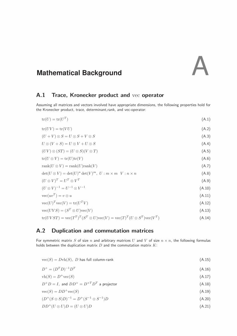
Mathematical Background AA.1 Trace, Kronecker product and vec operator
Assuming all matrices and vectors involved have appropriate dimensions, the following properties hold forthe Kronecker product, trace, determinant,rank, and vec-operator:
tr(U) = tr(UT ) (A.1)
tr(UV ) = tr(V U) (A.2)
(U + V )⊗ S = U ⊗ S + V ⊗ S (A.3)
U ⊗ (V + S) = U ⊗ V + U ⊗ S (A.4)
(UV )⊗ (ST ) = (U ⊗ S)(V ⊗ T ) (A.5)
tr(U ⊗ V ) = tr(U)tr(V ) (A.6)
rank(U ⊗ V ) = rank(U)rank(V ) (A.7)
det(U ⊗ V ) = det(U)n det(V )m, U : m×m V : n× n (A.8)
(U ⊗ V )T = UT ⊗ V T (A.9)
(U ⊗ V )−1 = U−1 ⊗ V −1 (A.10)
vec(uvT ) = v ⊗ u (A.11)
vec(U)T vec(V ) = tr(UT V ) (A.12)
vec(UV S) = (ST ⊗ U)vec(V ) (A.13)
tr(UV ST ) = vec(TT )T (ST ⊗ U)vec(V ) = vec(T )T (U ⊗ ST )vec(V T ) (A.14)
A.2 Duplication and commutation matrices
For symmetric matrix S of size n and arbitrary matrices U and V of size n × n, the following formulasholds between the duplication matrix D and the commutation matrix K:
vec(S) = Dvh(S), D has full column-rank (A.15)
D+ = (DT D)−1DT (A.16)
vh(S) = D+vec(S) (A.17)
D+D = I, and DD+ = D+T DT a projector (A.18)
vec(S) = DD+vec(S) (A.19)
(D+(S ⊗ S)D)−1 = D+(S−1 ⊗ S−1)D (A.20)
DD+(U ⊗ U)D = (U ⊗ U)D (A.21)
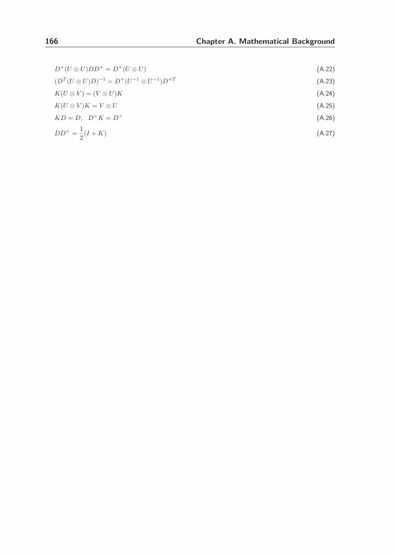
166 Chapter A. Mathematical Background
D+(U ⊗ U)DD+ = D+(U ⊗ U) (A.22)
(DT (U ⊗ U)D)−1 = D+(U−1 ⊗ U−1)D+T (A.23)
K(U ⊗ V ) = (V ⊗ U)K (A.24)
K(U ⊗ V )K = V ⊗ U (A.25)
KD = D, D+K = D+ (A.26)
DD+ =1
2(I + K) (A.27)

Derivation of Equations BB.1 Equation (5.116)
To see how the distribution of the w-test statistic looks like, we need the eigenvalues of CyQ−e in equa-
tion (5.82)
CyQ−e =
1
σ2
[0 00 Im
] [Q1 Q2
Q2 Q1
]
=1
σ2
[0 0Q2 Q1
]
(B.1)
with Q1 and Q2 as
q(1)ij =
2m−12m if i = j
−12m if i 6= j
, and q(2)ij =
−1
2m∀ i, j = 1, ...,m (B.2)
The matrix CyQ−e is of rank m, and we just need to compute the eigenvalues of the full rank matrix
1σ2 Q1; note that 1
σ2 Q1 is the block diagonal of Q−e . It can be rewritten as
1
σ2Q1 =
1
2σ2P1 +
1
2σ2Im (B.3)
with P1 an orthogonal projector of rank m− 1 and of the form
pij =
m−1m if i = j
−1m if i 6= j
(B.4)
The eigenvalues of 1σ2 Q1 then read
∣∣∣∣
1
σ2Q1 − γIm
∣∣∣∣=
∣∣∣∣
1
2σ2P1 − (γ − 1
2σ2)Im
∣∣∣∣= 0 (B.5)
or |P1 − (2σ2γ − 1)Im| = 0. Since P1 is a projector of rank m − 1, its eigenvalues read 2σ2γ1 − 1 =0, 2σ2γ2 − 1 = ... = 2σ2γm − 1 = 1, which yields
γ1 =1
2σ2, γ2 = ... = γm =
1
σ2(B.6)
This, with equation (5.82), wd =√
m−12σ2 and tr(CyQ−
e ) = 2m−12σ2 gives the 2m − 2 number of non-zero
eigenvalues λ as
λ1 = 0; λ2 = ... = λm =1
2√
m− 1; λm+1 = ... = λ2m−1 =
−1
2√
m− 1(B.7)
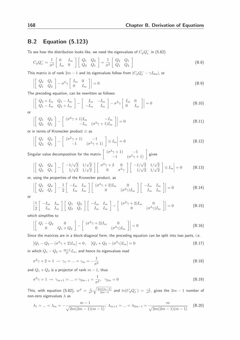
168 Chapter B. Derivation of Equations
B.2 Equation (5.123)
To see how the distribution looks like, we need the eigenvalues of CyQ−e in (5.82)
CyQ−e =
1
σ2
[0 Im
Im 0
] [Q1 Q2
Q2 Q1
]
=1
σ2
[Q2 Q1
Q1 Q2
]
(B.8)
This matrix is of rank 2m− 1 and its eigenvalues follow from |CyQ−e − γI2m|, or
∣∣∣∣
[Q2 Q1
Q1 Q2
]
− σ2γ
[Im 00 Im
]∣∣∣∣= 0 (B.9)
The preceding equation, can be rewritten as follows:∣∣∣∣
[Q2 + Im Q1 − Im
Q1 − Im Q2 + Im
]
−[
Im −Im
−Im Im
]
− σ2γ
[Im 00 Im
]∣∣∣∣= 0 (B.10)
or∣∣∣∣
[Q1 Q2
Q2 Q1
]
−[
(σ2γ + 1)Im −Im
−Im (σ2γ + 1)Im
]∣∣∣∣= 0 (B.11)
or in terms of Kronecker product ⊗ as∣∣∣∣
[Q1 Q2
Q2 Q1
]
−[
(σ2γ + 1) −1−1 (σ2γ + 1)
]
⊗ Im
∣∣∣∣= 0 (B.12)
Singular value decomposition for the matrix
[(σ2γ + 1) −1−1 (σ2γ + 1)
]
gives
∣∣∣∣
[Q1 Q2
Q2 Q1
]
−[−1/√
2 1/√
2
1/√
2 1/√
2
] [σ2γ + 2 0
0 σ2γ
] [−1/√
2 1/√
2
1/√
2 1/√
2
]
⊗ Im
∣∣∣∣= 0 (B.13)
or, using the properties of the Kronecker product, as∣∣∣∣
[Q1 Q2
Q2 Q1
]
− 1
2
[−Im Im
Im Im
] [(σ2γ + 2)Im 0
0 (σ2γ)Im
] [−Im Im
Im Im
]∣∣∣∣= 0 (B.14)
or∣∣∣∣
1
2
[−Im Im
Im Im
] [Q1 Q2
Q2 Q1
] [−Im Im
Im Im
]
−[
(σ2γ + 2)Im 00 (σ2γ)Im
]∣∣∣∣= 0 (B.15)
which simplifies to∣∣∣∣
[Q1 −Q2 0
0 Q1 + Q2
]
−[
(σ2γ + 2)Im 00 (σ2γ)Im
]∣∣∣∣= 0 (B.16)
Since the matrices are in a block-diagonal form, the preceding equation can be split into two parts, i.e.∣∣Q1 −Q2 − (σ2γ + 2)Im
∣∣ = 0 ,
∣∣Q1 + Q2 − (σ2γ)Im
∣∣ = 0 (B.17)
in which Q1 −Q2 = m−1m Im, and hence its eigenvalues read
σ2γ + 2 = 1 → γ1 = ... = γm = − 1
σ2(B.18)
and Q1 + Q2 is a projector of rank m− 1, thus
σ2γ = 1 → γm+1 = ... = γ2m−1 =1
σ2, γ2m = 0 (B.19)
This, with equation (5.82), wd = 1σ2
√2m(m−1)
2m−1 and tr(CyQ−e ) = −1
σ2 , gives the 2m − 1 number of
non-zero eigenvalues λ as
λ1 = ... = λm = − m− 1√
2m(2m− 1)(m− 1); λm+1 = ... = λ2m−1 =
m√
2m(2m− 1)(m− 1)(B.20)
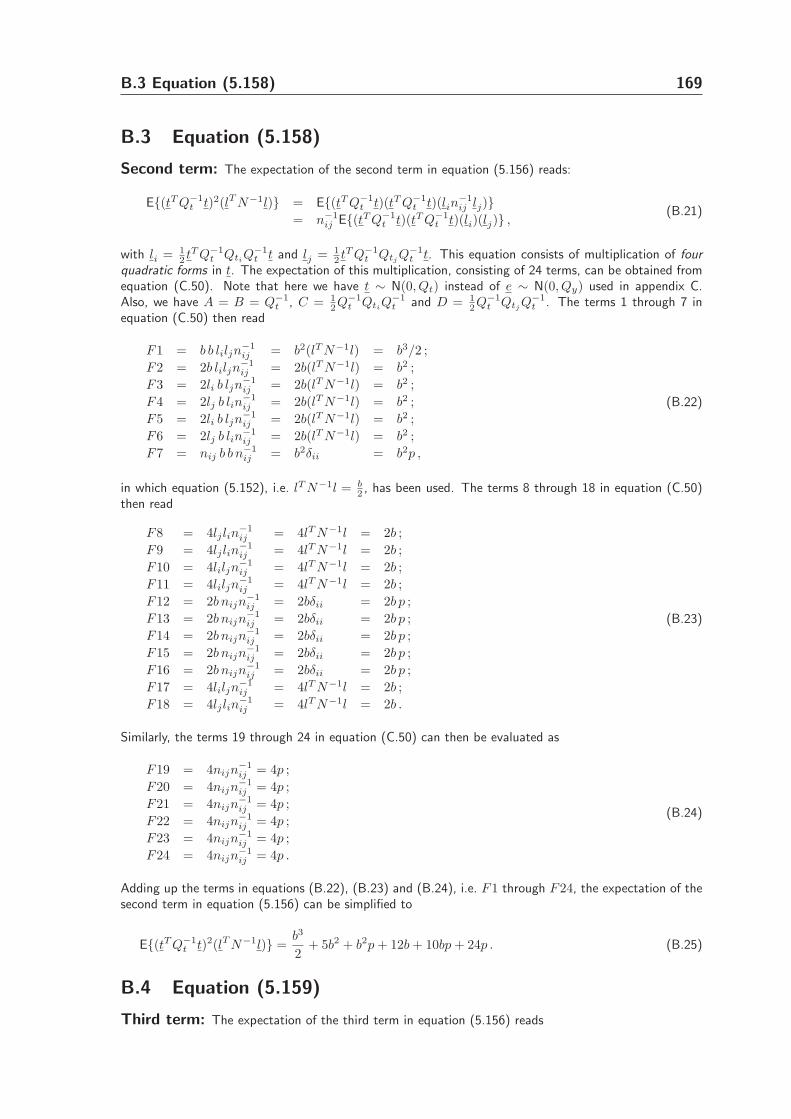
B.3 Equation (5.158) 169
B.3 Equation (5.158)
Second term: The expectation of the second term in equation (5.156) reads:
E{(tT Q−1t t)2(lT N−1l)} = E{(tT Q−1
t t)(tT Q−1t t)(lin
−1ij lj)}
= n−1ij E{(tT Q−1
t t)(tT Q−1t t)(li)(lj)} ,
(B.21)
with li = 12 tT Q−1
t QtiQ−1
t t and lj = 12 tT Q−1
t QtjQ−1
t t. This equation consists of multiplication of fourquadratic forms in t. The expectation of this multiplication, consisting of 24 terms, can be obtained fromequation (C.50). Note that here we have t ∼ N(0, Qt) instead of e ∼ N(0, Qy) used in appendix C.Also, we have A = B = Q−1
t , C = 12Q−1
t QtiQ−1
t and D = 12Q−1
t QtjQ−1
t . The terms 1 through 7 inequation (C.50) then read
F1 = b b liljn−1ij = b2(lT N−1l) = b3/2 ;
F2 = 2b liljn−1ij = 2b(lT N−1l) = b2 ;
F3 = 2li b ljn−1ij = 2b(lT N−1l) = b2 ;
F4 = 2lj b lin−1ij = 2b(lT N−1l) = b2 ;
F5 = 2li b ljn−1ij = 2b(lT N−1l) = b2 ;
F6 = 2lj b lin−1ij = 2b(lT N−1l) = b2 ;
F7 = nij b b n−1ij = b2δii = b2p ,
(B.22)
in which equation (5.152), i.e. lT N−1l = b2 , has been used. The terms 8 through 18 in equation (C.50)
then read
F8 = 4lj lin−1ij = 4lT N−1l = 2b ;
F9 = 4lj lin−1ij = 4lT N−1l = 2b ;
F10 = 4liljn−1ij = 4lT N−1l = 2b ;
F11 = 4liljn−1ij = 4lT N−1l = 2b ;
F12 = 2b nijn−1ij = 2bδii = 2b p ;
F13 = 2b nijn−1ij = 2bδii = 2b p ;
F14 = 2b nijn−1ij = 2bδii = 2b p ;
F15 = 2b nijn−1ij = 2bδii = 2b p ;
F16 = 2b nijn−1ij = 2bδii = 2b p ;
F17 = 4liljn−1ij = 4lT N−1l = 2b ;
F18 = 4lj lin−1ij = 4lT N−1l = 2b .
(B.23)
Similarly, the terms 19 through 24 in equation (C.50) can then be evaluated as
F19 = 4nijn−1ij = 4p ;
F20 = 4nijn−1ij = 4p ;
F21 = 4nijn−1ij = 4p ;
F22 = 4nijn−1ij = 4p ;
F23 = 4nijn−1ij = 4p ;
F24 = 4nijn−1ij = 4p .
(B.24)
Adding up the terms in equations (B.22), (B.23) and (B.24), i.e. F1 through F24, the expectation of thesecond term in equation (5.156) can be simplified to
E{(tT Q−1t t)2(lT N−1l)} =
b3
2+ 5b2 + b2p + 12b + 10bp + 24p . (B.25)
B.4 Equation (5.159)
Third term: The expectation of the third term in equation (5.156) reads
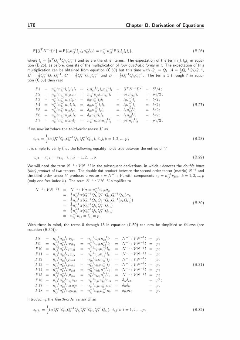
170 Chapter B. Derivation of Equations
E{(lT N−1l)2} = E{lin−1ij lj lkn−1
kl ll} = n−1ij n−1
kl E{lilj lkll} , (B.26)
where li = 12 tT Q−1
t QtiQ−1
t t and so are the other terms. The expectation of the term lilj lkll in equa-tion (B.26), as before, consists of the multiplication of four quadratic forms in t. The expectation of thismultiplication can be obtained from equation (C.50) but this time with Qy = Qt, A = 1
2Q−1t Qti
Q−1t ,
B = 12Q−1
t QtjQ−1
t , C = 12Q−1
t QtkQ−1
t and D = 12Q−1
t QtlQ−1
t . The terms 1 through 7 in equa-tion (C.50) then read
F1 = n−1ij n−1
kl lilj lkll = lin−1ij lj lkn−1
kl ll = (lT N−1l)2 = b2/4 ;
F2 = n−1ij n−1
kl nij lkll = n−1ij njilkn−1
kl ll = p lkn−1kl ll = p b/2 ;
F3 = n−1ij n−1
kl niklj ll = δiln−1ij lj ll = lin
−1ij lj = b/2 ;
F4 = n−1ij n−1
kl nillj lk = δikn−1ij lj lk = lin
−1ij lj = b/2 ;
F5 = n−1ij n−1
kl njklill = δikn−1kl lill = lkn−1
kl ll = b/2 ;
F6 = n−1ij n−1
kl njllilk = δiln−1kl lilk = lkn−1
kl ll = b/2 ;
F7 = n−1ij n−1
kl nkllilj = n−1kl nlklin
−1ij lj = p lin
−1ij lj = p b/2 .
(B.27)
If we now introduce the third-order tensor V as
vijk =1
2tr(Q−1
t QtiQ−1
t QtjQ−1
t Qtk), i, j, k = 1, 2, ..., p , (B.28)
it is simple to verify that the following equality holds true between the entries of V
vijk = vjki = vkij , i, j, k = 1, 2, ..., p . (B.29)
We will need the term N−1 : V N−1l in the subsequent derivations, in which : denotes the double inner(dot) product of two tensors. The double dot product between the second order tensor (matrix) N−1 andthe third order tensor V produces a vector s = N−1 : V , with components sk = n−1
ij vjik, k = 1, 2, ..., p
(only one free index k). The term N−1 : V N−1l simplifies to
N−1 : V N−1l = N−1 : V σ = n−1ij vijkσk
= 12n−1
ij tr(Q−1t Qti
Q−1t Qtj
Q−1t Qtk
)σk
= 12n−1
ij tr(Q−1t Qti
Q−1t Qtj
Q−1t [σkQtk
])
= 12n−1
ij tr(Q−1t Qti
Q−1t Qtj
)
= 12n−1
ij tr(Q−1t Qti
Q−1t Qtj
)
= n−1ij nij = δii = p .
(B.30)
With these in mind, the terms 8 through 18 in equation (C.50) can now be simplified as follows (seeequation (B.30)):
F8 = n−1ij n−1
kl llvijk = n−1ji vijkn−1
kl ll = N−1 : V N−1l = p ;
F9 = n−1ij n−1
kl llvikj = n−1ij vjikn−1
kl ll = N−1 : V N−1l = p ;
F10 = n−1ij n−1
kl lkvijl = n−1ji vijln
−1lk lk = N−1 : V N−1l = p ;
F11 = n−1ij n−1
kl lkvilj = n−1ij vjiln
−1lk lk = N−1 : V N−1l = p ;
F12 = n−1ij n−1
kl ljvikl = n−1lk vklin
−1ij lj = N−1 : V N−1l = p ;
F13 = n−1ij n−1
kl ljvilk = n−1kl vlkin
−1ij lj = N−1 : V N−1l = p ;
F14 = n−1ij n−1
kl livjkl = n−1lk vkljn
−1ji li = N−1 : V N−1l = p ;
F15 = n−1ij n−1
kl livjlk = n−1kl vlkjn
−1ji li = N−1 : V N−1l = p ;
F16 = n−1ij n−1
kl nijnkl = n−1ij njin
−1kl nlk = δiiδkk = p2 ;
F17 = n−1ij n−1
kl niknjl = n−1ij njln
−1lk nki = δilδli = p ;
F18 = n−1ij n−1
kl nilnjk = n−1ij njkn−1
kl nli = δikδki = p .
(B.31)
Introducing the fourth-order tensor Z as
zijkl =1
2tr(Q−1
t QtiQ−1
t QtjQ−1
t QtkQ−1
t Qtl), i, j, k, l = 1, 2, ..., p , (B.32)
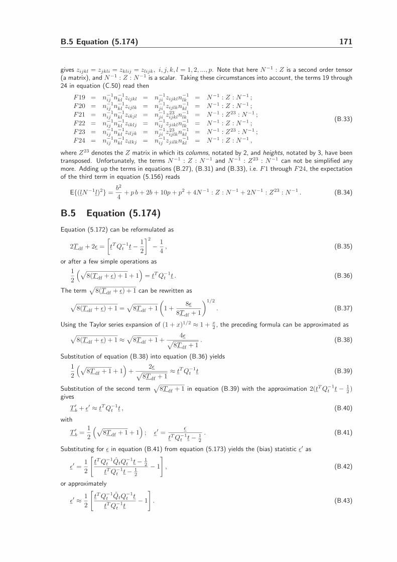
B.5 Equation (5.174) 171
gives zijkl = zjkli = zklij = zlijk, i, j, k, l = 1, 2, ..., p. Note that here N−1 : Z is a second order tensor(a matrix), and N−1 : Z : N−1 is a scalar. Taking these circumstances into account, the terms 19 through24 in equation (C.50) read then
F19 = n−1ij n−1
kl zijkl = n−1ji zijkln
−1lk = N−1 : Z : N−1 ;
F20 = n−1ij n−1
kl zijlk = n−1ji zijlkn−1
kl = N−1 : Z : N−1 ;
F21 = n−1ij n−1
kl zikjl = n−1ji z23
ijkln−1lk = N−1 : Z23 : N−1 ;
F22 = n−1ij n−1
kl ziklj = n−1ij zjikln
−1lk = N−1 : Z : N−1 ;
F23 = n−1ij n−1
kl ziljk = n−1ji z23
ijlkn−1kl = N−1 : Z23 : N−1 ;
F24 = n−1ij n−1
kl zilkj = n−1ij zjilkn−1
kl = N−1 : Z : N−1 ,
(B.33)
where Z23 denotes the Z matrix in which its columns, notated by 2, and heights, notated by 3, have beentransposed. Unfortunately, the terms N−1 : Z : N−1 and N−1 : Z23 : N−1 can not be simplified anymore. Adding up the terms in equations (B.27), (B.31) and (B.33), i.e. F1 through F24, the expectationof the third term in equation (5.156) reads
E{(lN−1l)2} =b2
4+ p b + 2b + 10p + p2 + 4N−1 : Z : N−1 + 2N−1 : Z23 : N−1 . (B.34)
B.5 Equation (5.174)
Equation (5.172) can be reformulated as
2T df + 2ǫ =
[
tT Q−1t t− 1
2
]2
− 1
4, (B.35)
or after a few simple operations as
1
2
(√
8(T df + ǫ) + 1 + 1)
= tT Q−1t t . (B.36)
The term√
8(T df + ǫ) + 1 can be rewritten as
√
8(T df + ǫ) + 1 =√
8T df + 1
(
1 +8ǫ
8T df + 1
)1/2
. (B.37)
Using the Taylor series expansion of (1 + x)1/2 ≈ 1 + x2 , the preceding formula can be approximated as
√
8(T df + ǫ) + 1 ≈√
8T df + 1 +4ǫ
√8T df + 1
. (B.38)
Substitution of equation (B.38) into equation (B.36) yields
1
2
(√
8T df + 1 + 1)
+2ǫ
√8T df + 1
≈ tT Q−1t t (B.39)
Substitution of the second term√
8T df + 1 in equation (B.39) with the approximation 2(tT Q−1t t − 1
2 )gives
T ′b + ǫ′ ≈ tT Q−1
t t , (B.40)
with
T ′b =
1
2
(√
8T df + 1 + 1)
; ǫ′ =ǫ
tT Q−1t t− 1
2
. (B.41)
Substituting for ǫ in equation (B.41) from equation (5.173) yields the (bias) statistic ǫ′ as
ǫ′ =1
2
[
tT Q−1t QtQ
−1t t− 1
2
tT Q−1t t− 1
2
− 1
]
, (B.42)
or approximately
ǫ′ ≈ 1
2
[
tT Q−1t QtQ
−1t t
tT Q−1t t
− 1
]
. (B.43)

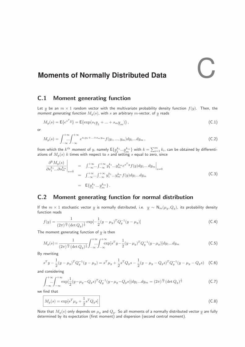
Moments of Normally Distributed Data CC.1 Moment generating function
Let y be an m × 1 random vector with the multivariate probability density function f(y). Then, themoment generating function My(s), with s an arbitrary m-vector, of y reads
My(s) = E{esT y} = E{exp(s1y1+ ... + smy
m)} , (C.1)
or
My(s) =
∫ +∞
−∞...
∫ +∞
−∞es1y1+...+smymf(y1, ..., ym)dy1...dym , (C.2)
from which the kth moment of y, namely E{yk1
1...ykm
m} with k =
∑mi=1 ki, can be obtained by differenti-
ations of My(s) k times with respect to s and setting s equal to zero, since
∂kMy(s)
∂sk1
1 ...∂skmm
∣∣∣∣∣s=0
=∫ +∞−∞...
∫ +∞−∞ yk1
1 ...ykmm esT yf(y)dy1... dym
∣∣∣s=0
=∫ +∞−∞...
∫ +∞−∞ yk1
1 ...ykmm f(y)dy1...dym
= E{yk1
1... ykm
m} .
(C.3)
C.2 Moment generating function for normal distribution
If the m × 1 stochastic vector y is normally distributed, i.e. y ∼ Nm(µy, Qy), its probability densityfunction reads
f(y) =1
(2π)m2 (detQy)
1
2
exp[−1
2(y − µy)T Q−1
y (y − µy)] (C.4)
The moment generating function of y is then
My(s)=1
(2π)m2 (detQy)
1
2
∫ +∞
−∞...
∫ +∞
−∞exp[sT y− 1
2(y−µy)T Q−1
y (y−µy)]dy1...dym (C.5)
By rewriting
sT y − 1
2(y − µy)T Q−1
y (y − µy) = sT µy +1
2sT Qys− 1
2(y − µy −Qys)T Q−1
y (y − µy −Qys) (C.6)
and considering∫ +∞
−∞...
∫ +∞
−∞exp[
1
2(y−µy−Qys)T Q−1
y (y−µy−Qys)]dy1...dym = (2π)m2 (detQy)
1
2 (C.7)
we find that
My(s) = exp[sT µy +1
2sT Qys] (C.8)
Note that My(s) only depends on µy and Qy. So all moments of a normally distributed vector y are fullydetermined by its expectation (first moment) and dispersion (second central moment).
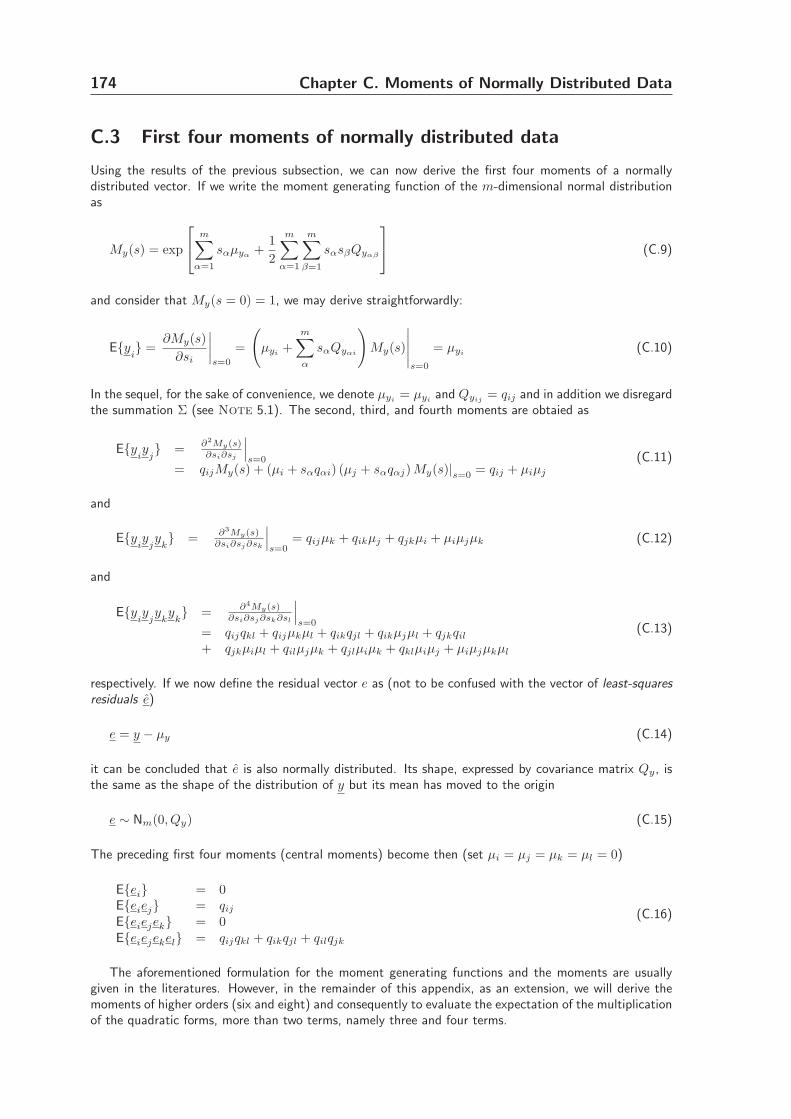
174 Chapter C. Moments of Normally Distributed Data
C.3 First four moments of normally distributed data
Using the results of the previous subsection, we can now derive the first four moments of a normallydistributed vector. If we write the moment generating function of the m-dimensional normal distributionas
My(s) = exp
m∑
α=1
sαµyα+
1
2
m∑
α=1
m∑
β=1
sαsβQyαβ
(C.9)
and consider that My(s = 0) = 1, we may derive straightforwardly:
E{yi} =
∂My(s)
∂si
∣∣∣∣s=0
=
(
µyi+
m∑
α
sαQyαi
)
My(s)
∣∣∣∣∣s=0
= µyi(C.10)
In the sequel, for the sake of convenience, we denote µyi= µyi
and Qyij= qij and in addition we disregard
the summation Σ (see Note 5.1). The second, third, and fourth moments are obtaied as
E{yiy
j} =
∂2My(s)∂si∂sj
∣∣∣s=0
= qijMy(s) + (µi + sαqαi) (µj + sαqαj) My(s)|s=0 = qij + µiµj
(C.11)
and
E{yiy
jy
k} =
∂3My(s)∂si∂sj∂sk
∣∣∣s=0
= qijµk + qikµj + qjkµi + µiµjµk (C.12)
and
E{yiy
jy
ky
k} =
∂4My(s)∂si∂sj∂sk∂sl
∣∣∣s=0
= qijqkl + qijµkµl + qikqjl + qikµjµl + qjkqil
+ qjkµiµl + qilµjµk + qjlµiµk + qklµiµj + µiµjµkµl
(C.13)
respectively. If we now define the residual vector e as (not to be confused with the vector of least-squaresresiduals e)
e = y − µy (C.14)
it can be concluded that e is also normally distributed. Its shape, expressed by covariance matrix Qy, isthe same as the shape of the distribution of y but its mean has moved to the origin
e ∼ Nm(0, Qy) (C.15)
The preceding first four moments (central moments) become then (set µi = µj = µk = µl = 0)
E{ei} = 0E{eiej} = qij
E{eiejek} = 0E{eiejekel} = qijqkl + qikqjl + qilqjk
(C.16)
The aforementioned formulation for the moment generating functions and the moments are usuallygiven in the literatures. However, in the remainder of this appendix, as an extension, we will derive themoments of higher orders (six and eight) and consequently to evaluate the expectation of the multiplicationof the quadratic forms, more than two terms, namely three and four terms.
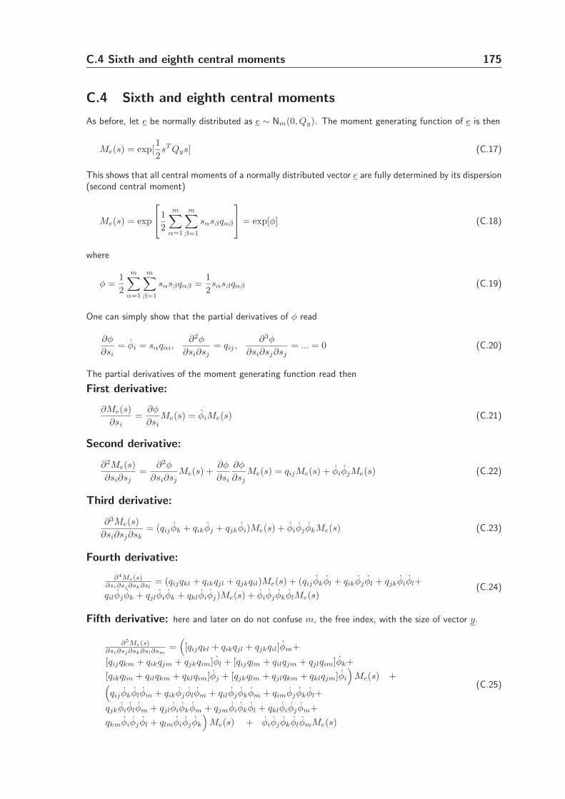
C.4 Sixth and eighth central moments 175
C.4 Sixth and eighth central moments
As before, let e be normally distributed as e ∼ Nm(0, Qy). The moment generating function of e is then
Me(s) = exp[1
2sT Qys] (C.17)
This shows that all central moments of a normally distributed vector e are fully determined by its dispersion(second central moment)
Me(s) = exp
1
2
m∑
α=1
m∑
β=1
sαsβqαβ
= exp[φ] (C.18)
where
φ =1
2
m∑
α=1
m∑
β=1
sαsβqαβ =1
2sαsβqαβ (C.19)
One can simply show that the partial derivatives of φ read
∂φ
∂si= φi = sαqαi,
∂2φ
∂si∂sj= qij ,
∂3φ
∂si∂sj∂sj= ... = 0 (C.20)
The partial derivatives of the moment generating function read then
First derivative:
∂Me(s)
∂si=
∂φ
∂siMe(s) = φiMe(s) (C.21)
Second derivative:
∂2Me(s)
∂si∂sj=
∂2φ
∂si∂sjMe(s) +
∂φ
∂si
∂φ
∂sjMe(s) = qijMe(s) + φiφjMe(s) (C.22)
Third derivative:
∂3Me(s)
∂si∂sj∂sk= (qij φk + qikφj + qjkφi)Me(s) + φiφj φkMe(s) (C.23)
Fourth derivative:
∂4Me(s)∂si∂sj∂sk∂sl
= (qijqkl + qikqjl + qjkqil)Me(s) + (qij φkφl + qikφj φl + qjkφiφl+
qilφj φk + qjlφiφk + qklφiφj)Me(s) + φiφj φkφlMe(s)(C.24)
Fifth derivative: here and later on do not confuse m, the free index, with the size of vector y.
∂5Me(s)∂si∂sj∂sk∂sl∂sm
=(
[qijqkl + qikqjl + qjkqil]φm+
[qijqkm + qikqjm + qjkqim]φl + [qijqlm + qilqjm + qjlqim]φk+
[qikqlm + qilqkm + qklqim]φj + [qjkqlm + qjlqkm + qklqjm]φi
)
Me(s) +(
qij φkφlφm + qikφj φlφm + qilφj φkφm + qimφj φkφl+
qjkφiφlφm + qjlφiφkφm + qjmφiφkφl + qklφiφj φm+
qkmφiφj φl + qlmφiφj φk
)
Me(s) + φiφj φkφlφmMe(s)
(C.25)
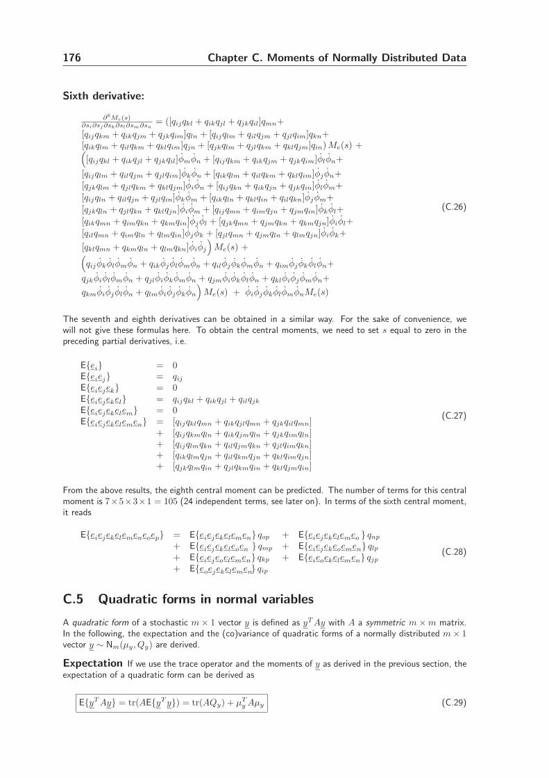
176 Chapter C. Moments of Normally Distributed Data
Sixth derivative:
∂6Me(s)∂si∂sj∂sk∂sl∂sm∂sn
= ([qijqkl + qikqjl + qjkqil]qmn+
[qijqkm + qikqjm + qjkqim]qln + [qijqlm + qilqjm + qjlqim]qkn+[qikqlm + qilqkm + qklqim]qjn + [qjkqlm + qjlqkm + qklqjm]qin) Me(s) +(
[qijqkl + qikqjl + qjkqil]φmφn + [qijqkm + qikqjm + qjkqim]φlφn+
[qijqlm + qilqjm + qjlqim]φkφn + [qikqlm + qilqkm + qklqim]φj φn+
[qjkqlm + qjlqkm + qklqjm]φiφn + [qijqkn + qikqjn + qjkqin]φlφm+
[qijqln + qilqjn + qjlqin]φkφm + [qikqln + qklqin + qilqkn]φj φm+
[qjkqln + qjlqkn + qklqjn]φiφm + [qijqmn + qimqjn + qjmqin]φkφl+
[qikqmn + qimqkn + qkmqin]φj φl + [qjkqmn + qjmqkn + qkmqjn]φiφl+
[qilqmn + qimqln + qlmqin]φj φk + [qjlqmn + qjmqln + qlmqjn]φiφk+
[qklqmn + qkmqln + qlmqkn]φiφj
)
Me(s) +(
qij φkφlφmφn + qikφj φlφmφn + qilφj φkφmφn + qimφj φkφlφn+
qjkφiφlφmφn + qjlφiφkφmφn + qjmφiφkφlφn + qklφiφj φmφn+
qkmφiφj φlφn + qlmφiφj φkφn
)
Me(s) + φiφj φkφlφmφnMe(s)
(C.26)
The seventh and eighth derivatives can be obtained in a similar way. For the sake of convenience, wewill not give these formulas here. To obtain the central moments, we need to set s equal to zero in thepreceding partial derivatives, i.e.
E{ei} = 0E{eiej} = qij
E{eiejek} = 0E{eiejekel} = qijqkl + qikqjl + qilqjk
E{eiejekelem} = 0E{eiejekelemen} = [qijqklqmn + qikqjlqmn + qjkqilqmn]
+ [qijqkmqln + qikqjmqln + qjkqimqln]+ [qijqlmqkn + qilqjmqkn + qjlqimqkn]+ [qikqlmqjn + qilqkmqjn + qklqimqjn]+ [qjkqlmqin + qjlqkmqin + qklqjmqin]
(C.27)
From the above results, the eighth central moment can be predicted. The number of terms for this centralmoment is 7×5×3×1 = 105 (24 independent terms, see later on). In terms of the sixth central moment,it reads
E{eiejekelemeneoep} = E{eiejekelemen} qop + E{eiejekelemeo } qnp
+ E{eiejekeleoen } qmp + E{eiejekeoemen} qlp
+ E{eiejeoelemen} qkp + E{eieoekelemen} qjp
+ E{eoejekelemen} qip
(C.28)
C.5 Quadratic forms in normal variables
A quadratic form of a stochastic m× 1 vector y is defined as yT Ay with A a symmetric m×m matrix.In the following, the expectation and the (co)variance of quadratic forms of a normally distributed m× 1vector y ∼ Nm(µy, Qy) are derived.
Expectation If we use the trace operator and the moments of y as derived in the previous section, theexpectation of a quadratic form can be derived as
E{yT Ay} = tr(AE{yT y}) = tr(AQy) + µTy Aµy (C.29)
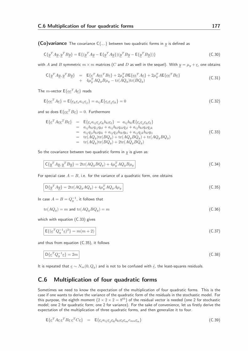
C.6 Multiplication of four quadratic forms 177
(Co)variance The covariance C{., .} between two quadratic forms in y is defined as
C{yT Ay, yT By} = E{(yT Ay − E{yT Ay})(yT By − E{yT By})} (C.30)
with A and B symmetric m×m matrices (C and D as well in the sequel). With y = µy + e, one obtains
C{yT Ay, yT By} = E{eT AeeT Be}+ 2µTy BE{eeT Ae}+ 2µT
y AE{eeT Be}+ 4µT
y AQyBµy − tr(AQy)tr(BQy)(C.31)
The m-vector E{eeT Ae} reads
E{eeT Ae} = E{ekeiaijej} = aijE{eiejek} = 0 (C.32)
and so does E{eeT Be} = 0. Furthermore
E{eT AeeT Be} = E{eiaijejekbklel} = aijbklE{eiejekel}= aijbklqijqkl + aijbklqikqjl + aijbklqilqjk
= aijqjibklqlk + aijqjlblkqki + aijqjkbklqli
= tr(AQy)tr(BQy) + tr(AQyBQy) + tr(AQyBQy)= tr(AQy)tr(BQy) + 2tr(AQyBQy)
(C.33)
So the covariance between two quadratic forms in y is given as:
C{yT Ay, yT By} = 2tr(AQyBQy) + 4µTy AQyBµy (C.34)
For special case A = B, i.e. for the variance of a quadratic form, one obtains
D{yT Ay} = 2tr(AQyAQy) + 4µTy AQyAµy (C.35)
In case A = B = Q−1y , it follows that
tr(AQy) = m and tr(AQyBQy) = m (C.36)
which with equation (C.33) gives
E{(eT Q−1y e)2} = m(m + 2) (C.37)
and thus from equation (C.35), it follows
D{eT Q−1y e} = 2m (C.38)
It is repeated that e ∼ Nm(0, Qy) and is not to be confused with e, the least-squares residuals.
C.6 Multiplication of four quadratic forms
Sometimes we need to know the expectation of the multiplication of four quadratic forms. This is thecase if one wants to derive the variance of the quadratic form of the residuals in the stochastic model. Forthis purpose, the eighth moment (2× 2× 2 = 8th) of the residual vector is needed (one 2 for stochasticmodel; one 2 for quadratic form; one 2 for variance). For the sake of convenience, let us firstly derive theexpectation of the multiplication of three quadratic forms, and then generalize it to four.
E{eT Ae eT Be eT Ce} = E{eiaijejekbklelemcmnen} (C.39)
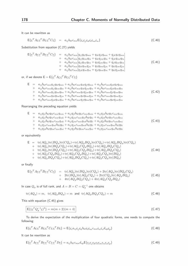
178 Chapter C. Moments of Normally Distributed Data
It can be rewritten as
E{eT Ae eT Be eT Ce} = aijbklcmnE{eiejekelemen} (C.40)
Substitution from equation (C.27) yields
E{eT Ae eT Be eT Ce} = aijbklcmn[qijqklqmn + qikqjlqmn + qjkqilqmn]+ aijbklcmn[qijqkmqln + qikqjmqln + qjkqimqln]+ aijbklcmn[qijqlmqkn + qilqjmqkn + qjlqimqkn]+ aijbklcmn[qikqlmqjn + qilqkmqjn + qklqimqjn]+ aijbklcmn[qjkqlmqin + qjlqkmqin + qklqjmqin]
(C.41)
or, if we denote E = E{eT Ae eT Be eT Ce}
E = aijbklcmnqijqklqmn + aijbklcmnqikqjlqmn + aijbklcmnqjkqilqmn
+ aijbklcmnqijqkmqln + aijbklcmnqikqjmqln + aijbklcmnqjkqimqln
+ aijbklcmnqijqlmqkn + aijbklcmnqilqjmqkn + aijbklcmnqjlqimqkn
+ aijbklcmnqikqlmqjn + aijbklcmnqilqkmqjn + aijbklcmnqklqimqjn
+ aijbklcmnqjkqlmqin + aijbklcmnqjlqkmqin + aijbklcmnqklqjmqin
(C.42)
Rearranging the preceding equation yields
E = aijqjibklqlkcmnqnm + aijqjlblkqkicmnqnm + aijqjkbklqlicmnqnm
+ aijqjibklqlncnmqmk + aijqjmcmnqnlblkqki + aijqjkbklqlncnmqmi
+ aijqjibklqlmcmnqnk + aijqjmcmnqnkbklqli + aijqjlblkqkncnmqmi
+ aijqjncnmqmlblkqki + aijqjncnmqmkbklqli + aijqjncnmqmibklqlk
+ aijqjkbklqlmcmnqni + aijqjlblkqkmcmnqni + aijqjmcmnqnibklqlk
(C.43)
or equivalently
E = tr(AQy)tr(BQy)tr(CQy)+tr(AQyBQy)tr(CQy)+tr(AQyBQy)tr(CQy)+ tr(AQy)tr(BQyCQy)+tr(AQyCQyBQy)+tr(AQyBQyCQy)+ tr(AQy)tr(BQyCQy)+tr(AQyCQyBQy)+tr(AQyBQyCQy)+ tr(AQyCQyBQy)+tr(AQyCQyBQy)+tr(AQyCQy)tr(BQy)+ tr(AQyBQyCQy)+tr(AQyBQyCQy)+tr(AQyCQy)tr(BQy)
(C.44)
or finally
E{eT Ae eT Be eT Ce} = tr(AQy)tr(BQy)tr(CQy) + 2tr(AQy)tr(BQyCQy)+ 2tr(BQy)tr(AQyCQy) + 2tr(CQy)tr(AQyBQy)+ 4tr(AQyBQyCQy) + 4tr(AQyCQyBQy)
(C.45)
In case Qy is of full rank, and A = B = C = Q−1y one obtains
tr(AQy) = m, tr(AQyBQy) = m and tr(AQyBQyCQy) = m (C.46)
This with equation (C.45) gives
E{(eT Q−1y e)3} = m(m + 2)(m + 4) (C.47)
To derive the expectation of the multiplication of four quadratic forms, one needs to compute thefollowing:
E{eT Ae eT Be eT Ce eT De} = E{eiaijejekbklelemcmneneodopep} (C.48)
It can be rewritten as
E{eT Ae eT Be eT Ce eT De} = aijbklcmndopE{eiejekelemeneoep} (C.49)
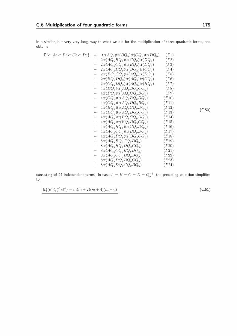
C.6 Multiplication of four quadratic forms 179
In a similar, but very very long, way to what we did for the multiplication of three quadratic forms, oneobtains
E{eT Ae eT Be eT Ce eT De} = tr(AQy)tr(BQy)tr(CQy)tr(DQy) (F1)+ 2tr(AQyBQy)tr(CQy)tr(DQy) (F2)+ 2tr(AQyCQy)tr(BQy)tr(DQy) (F3)+ 2tr(AQyDQy)tr(BQy)tr(CQy) (F4)+ 2tr(BQyCQy)tr(AQy)tr(DQy) (F5)+ 2tr(BQyDQy)tr(AQy)tr(CQy) (F6)+ 2tr(CQyDQy)tr(AQy)tr(BQy) (F7)+ 4tr(DQy)tr(AQyBQyCQy) (F8)+ 4tr(DQy)tr(AQyCQyBQy) (F9)+ 4tr(CQy)tr(AQyBQyDQy) (F10)+ 4tr(CQy)tr(AQyDQyBQy) (F11)+ 4tr(BQy)tr(AQyCQyDQy) (F12)+ 4tr(BQy)tr(AQyDQyCQy) (F13)+ 4tr(AQy)tr(BQyCQyDQy) (F14)+ 4tr(AQy)tr(BQyDQyCQy) (F15)+ 4tr(AQyBQy)tr(CQyDQy) (F16)+ 4tr(AQyCQy)tr(BQyDQy) (F17)+ 4tr(AQyDQy)tr(BQyCQy) (F18)+ 8tr(AQyBQyCQyDQy) (F19)+ 8tr(AQyBQyDQyCQy) (F20)+ 8tr(AQyCQyBQyDQy) (F21)+ 8tr(AQyCQyDQyBQy) (F22)+ 8tr(AQyDQyBQyCQy) (F23)+ 8tr(AQyDQyCQyBQy) (F24)
(C.50)
consisting of 24 independent terms. In case A = B = C = D = Q−1y , the preceding equation simplifies
to
E{(eT Q−1y e)4} = m(m + 2)(m + 4)(m + 6) (C.51)

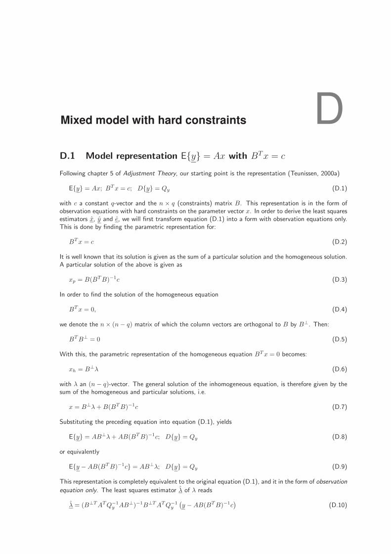
Mixed model with hard constraints DD.1 Model representation E{y} = Ax with BTx = c
Following chapter 5 of Adjustment Theory, our starting point is the representation (Teunissen, 2000a)
E{y} = Ax; BT x = c; D{y} = Qy (D.1)
with c a constant q-vector and the n × q (constraints) matrix B. This representation is in the form ofobservation equations with hard constraints on the parameter vector x. In order to derive the least squaresestimators x, y and e, we will first transform equation (D.1) into a form with observation equations only.This is done by finding the parametric representation for:
BT x = c (D.2)
It is well known that its solution is given as the sum of a particular solution and the homogeneous solution.A particular solution of the above is given as
xp = B(BT B)−1c (D.3)
In order to find the solution of the homogeneous equation
BT x = 0, (D.4)
we denote the n× (n− q) matrix of which the column vectors are orthogonal to B by B⊥. Then:
BT B⊥ = 0 (D.5)
With this, the parametric representation of the homogeneous equation BT x = 0 becomes:
xh = B⊥λ (D.6)
with λ an (n− q)-vector. The general solution of the inhomogeneous equation, is therefore given by thesum of the homogeneous and particular solutions, i.e.
x = B⊥λ + B(BT B)−1c (D.7)
Substituting the preceding equation into equation (D.1), yields
E{y} = AB⊥λ + AB(BT B)−1c; D{y} = Qy (D.8)
or equivalently
E{y −AB(BT B)−1c} = AB⊥λ; D{y} = Qy (D.9)
This representation is completely equivalent to the original equation (D.1), and it in the form of observation
equation only. The least squares estimator λ of λ reads
λ = (B⊥T AT Q−1y AB⊥)−1B⊥T AT Q−1
y
(y −AB(BT B)−1c
)(D.10)
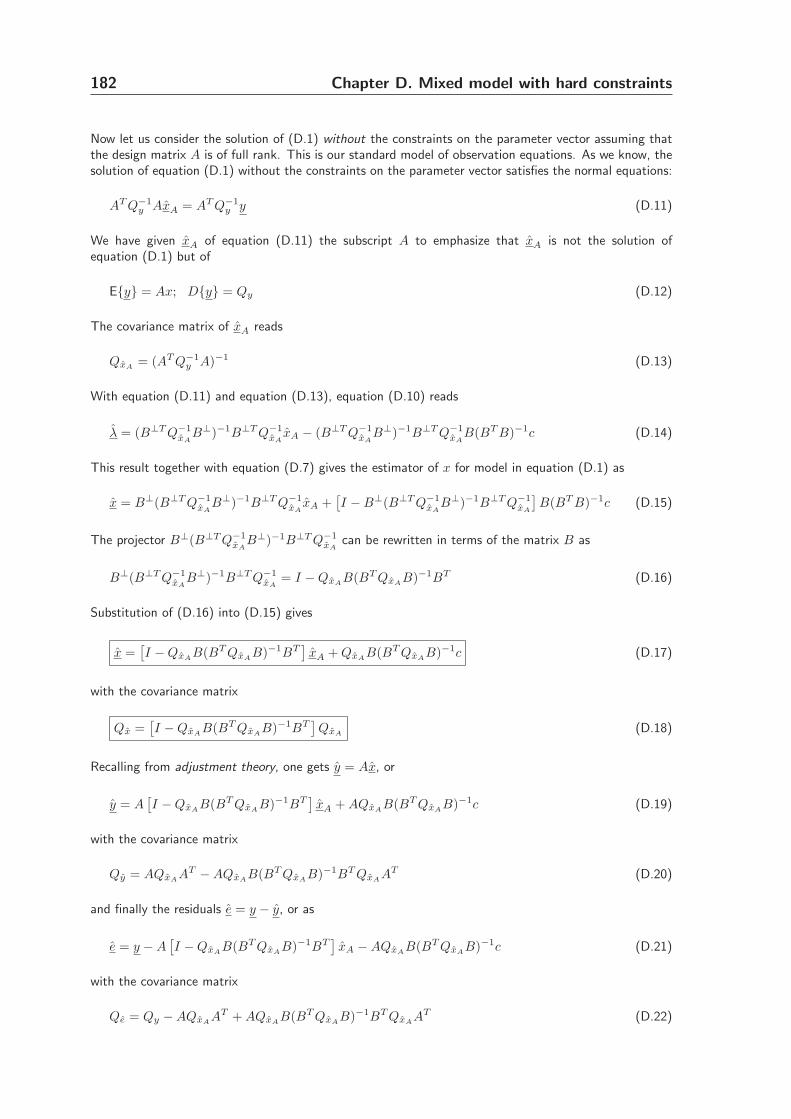
182 Chapter D. Mixed model with hard constraints
Now let us consider the solution of (D.1) without the constraints on the parameter vector assuming thatthe design matrix A is of full rank. This is our standard model of observation equations. As we know, thesolution of equation (D.1) without the constraints on the parameter vector satisfies the normal equations:
AT Q−1y AxA = AT Q−1
y y (D.11)
We have given xA of equation (D.11) the subscript A to emphasize that xA is not the solution ofequation (D.1) but of
E{y} = Ax; D{y} = Qy (D.12)
The covariance matrix of xA reads
QxA= (AT Q−1
y A)−1 (D.13)
With equation (D.11) and equation (D.13), equation (D.10) reads
λ = (B⊥T Q−1xA
B⊥)−1B⊥T Q−1xA
xA − (B⊥T Q−1xA
B⊥)−1B⊥T Q−1xA
B(BT B)−1c (D.14)
This result together with equation (D.7) gives the estimator of x for model in equation (D.1) as
x = B⊥(B⊥T Q−1xA
B⊥)−1B⊥T Q−1xA
xA +[I −B⊥(B⊥T Q−1
xAB⊥)−1B⊥T Q−1
xA
]B(BT B)−1c (D.15)
The projector B⊥(B⊥T Q−1xA
B⊥)−1B⊥T Q−1xA
can be rewritten in terms of the matrix B as
B⊥(B⊥T Q−1xA
B⊥)−1B⊥T Q−1xA
= I −QxAB(BT QxA
B)−1BT (D.16)
Substitution of (D.16) into (D.15) gives
x =[I −QxA
B(BT QxAB)−1BT
]xA + QxA
B(BT QxAB)−1c (D.17)
with the covariance matrix
Qx =[I −QxA
B(BT QxAB)−1BT
]QxA
(D.18)
Recalling from adjustment theory, one gets y = Ax, or
y = A[I −QxA
B(BT QxAB)−1BT
]xA + AQxA
B(BT QxAB)−1c (D.19)
with the covariance matrix
Qy = AQxAAT −AQxA
B(BT QxAB)−1BT QxA
AT (D.20)
and finally the residuals e = y − y, or as
e = y −A[I −QxA
B(BT QxAB)−1BT
]xA −AQxA
B(BT QxAB)−1c (D.21)
with the covariance matrix
Qe = Qy −AQxAAT + AQxA
B(BT QxAB)−1BT QxA
AT (D.22)
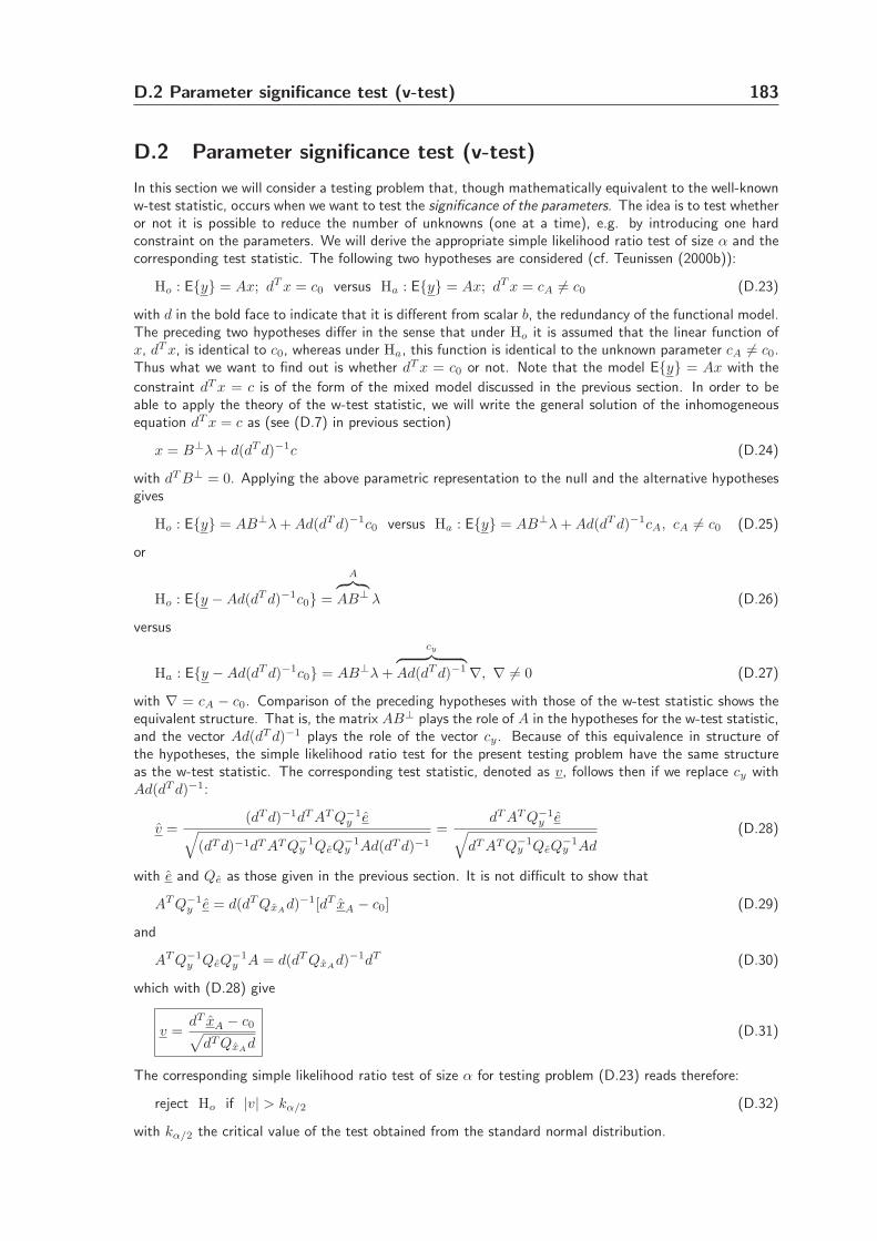
D.2 Parameter significance test (v-test) 183
D.2 Parameter significance test (v-test)
In this section we will consider a testing problem that, though mathematically equivalent to the well-knownw-test statistic, occurs when we want to test the significance of the parameters. The idea is to test whetheror not it is possible to reduce the number of unknowns (one at a time), e.g. by introducing one hardconstraint on the parameters. We will derive the appropriate simple likelihood ratio test of size α and thecorresponding test statistic. The following two hypotheses are considered (cf. Teunissen (2000b)):
Ho : E{y} = Ax; dT x = c0 versus Ha : E{y} = Ax; dT x = cA 6= c0 (D.23)
with d in the bold face to indicate that it is different from scalar b, the redundancy of the functional model.The preceding two hypotheses differ in the sense that under Ho it is assumed that the linear function ofx, dT x, is identical to c0, whereas under Ha, this function is identical to the unknown parameter cA 6= c0.Thus what we want to find out is whether dT x = c0 or not. Note that the model E{y} = Ax with the
constraint dT x = c is of the form of the mixed model discussed in the previous section. In order to beable to apply the theory of the w-test statistic, we will write the general solution of the inhomogeneousequation dT x = c as (see (D.7) in previous section)
x = B⊥λ + d(dT d)−1c (D.24)
with dT B⊥ = 0. Applying the above parametric representation to the null and the alternative hypothesesgives
Ho : E{y} = AB⊥λ + Ad(dT d)−1c0 versus Ha : E{y} = AB⊥λ + Ad(dT d)−1cA, cA 6= c0 (D.25)
or
Ho : E{y −Ad(dT d)−1c0} =
A︷ ︸︸ ︷
AB⊥ λ (D.26)
versus
Ha : E{y −Ad(dT d)−1c0} = AB⊥λ +
cy
︷ ︸︸ ︷
Ad(dT d)−1∇, ∇ 6= 0 (D.27)
with ∇ = cA − c0. Comparison of the preceding hypotheses with those of the w-test statistic shows theequivalent structure. That is, the matrix AB⊥ plays the role of A in the hypotheses for the w-test statistic,and the vector Ad(dT d)−1 plays the role of the vector cy. Because of this equivalence in structure ofthe hypotheses, the simple likelihood ratio test for the present testing problem have the same structureas the w-test statistic. The corresponding test statistic, denoted as v, follows then if we replace cy withAd(dT d)−1:
v =(dT d)−1dT AT Q−1
y e√
(dT d)−1dT AT Q−1y QeQ
−1y Ad(dT d)−1
=dT AT Q−1
y e√
dT AT Q−1y QeQ
−1y Ad
(D.28)
with e and Qe as those given in the previous section. It is not difficult to show that
AT Q−1y e = d(dT QxA
d)−1[dT xA − c0] (D.29)
and
AT Q−1y QeQ
−1y A = d(dT QxA
d)−1dT (D.30)
which with (D.28) give
v =dT xA − c0√
dT QxAd
(D.31)
The corresponding simple likelihood ratio test of size α for testing problem (D.23) reads therefore:
reject Ho if |v| > kα/2 (D.32)
with kα/2 the critical value of the test obtained from the standard normal distribution.

184 Chapter D. Mixed model with hard constraints
D.3 Derivation of w-test from v-test statistic
Let us consider the following two hypotheses
Ho : E{y} = Ax, versus Ha : E{y} = Ax + cy∇, and ∇ 6= 0 (D.33)
In order to obtain the well-known w-test statistic from the v-test presented in the previous section, wemay reformulate equation (D.33) as
Ho : E{y} = [Acy]
[x∇
]
, ∇ = 0 versus Ha : E{y} = [Acy]
[x∇
]
, ∇ 6= 0 (D.34)
This formulation is identical to equation (D.23) with
b = [0, ..., 0, 1]T , c0 = 0 (D.35)
The least squares solution of the model E{y} = [Acy]
[x∇
]
read
[x
∇
]
=
[AT Q−1
y A AT Q−1y cy
cTy Q−1
y A cTy Q−1
y cy
]−1 [AT Q−1
y ycTy Q−1
y y
]
(D.36)
The inverse of the normal matrix reads then
[AT Q−1
y A AT Q−1y cy
cTy Q−1
y A cTy Q−1
y cy
]−1
=
[N−1
11 N−112
N−121 N−1
22
]
(D.37)
with
N−111 = (AT Q−1
y A)−1 − σ2∇(AT Q−1
y A)−1AT Q−1y cycT
y Q−1y A(AT Q−1
y A)−1
N−112 = −σ2
∇.(AT Q−1y A)−1AT Q−1
y cy
N−121 = −σ2
∇.cTy Q−1
y A(AT Q−1y A)−1
N−122 = σ2
∇
(D.38)
with
σ2∇ = (cyQ−1
y cy − cyQ−1y A(AT Q−1
y A)−1AT Q−1y cy)−1
= (cyQ−1y (I −A(AT Q−1
y A)−1AT Q−1y )cy)−1
= (cyQ−1y P⊥
A cy)−1
=∥∥P⊥
A cy
∥∥−2
Q−1y
(D.39)
The estimator ∇ can be obtained as
∇ = N−121 AT Q−1
y y + N−122 cT
y Q−1y y
= σ2∇cT
y Q−1y y − σ2
∇.cTy Q−1
y A(AT Q−1y A)−1AT Q−1
y y
= σ2∇cT
y Q−1y
(I −A(AT Q−1
y A)−1AT Q−1y
)y
= σ2∇cT
y Q−1y P⊥
A y
(D.40)
The v-test statistic (D.31), denoted here as w-test statistic, with equation (D.35), can be written as
w =∇σ∇
(D.41)
which with equations (D.39) and (D.40) proves the claim
w =cTy Q−1
y P⊥A y
∥∥P⊥
A cy
∥∥
Q−1y
(D.42)
Bibliography
Abbasi M (1999). Comparison of Fourier, least-squares and wavelet spectral analysis meth-ods, tested on Persian Gulf tidal data. MSc thesis, Surveying Engineering Department,K.N. Toosi University of Technology, Tehran, Iran.
Agnew D (1992). The time domain behavior of power law noises. Geophysical ResearchLetters, 19: 333–336.
Agnew DC, Larson KM (2007). Finding the repeat times of the GPS constellation. GPSSolutions, 11(1): 71–76.
Altamimi Z, Sillard P, Boucher C (2002). ITRF2000: A new release of the International Ter-restrial Reference Frame for earth science applications. Journal of Geophysical Research,107(B10, 2214).
Amiri-Simkooei AR (2003). Formulation of L1 norm minimization in Gauss-Markov models.Journal of Surveying Engineering , 129(1): 37–43.
Amiri-Simkooei AR (2005). Separating receiver noise and multipath effects in time seriesof GPS baselines using harmonic functions. In ION GNSS 18th International TechnicalMeeting of the Satellite Division, September 13-16 2005, Long Beach, CA, pp. 1034–1045. (sponsored student paper).
Amiri-Simkooei AR, Tiberius CCJM (2007). Assessing receiver noise using GPS shortbaseline time series. GPS Solutions, 11(1): 21–35.
Amiri-Simkooei AR, Tiberius CCJM, Teunissen PJG (2006). Assessment of noise in GPScoordinate time series: methodology and results. Journal of Geophysical Research,submitted.
Asgari J, Harmel A (2005). Least squares spectral analysis of GPS derived ionosphericdata. In The ION National Technical Meeting, Jan. 24-26 San Diego, California.
Baarda W (1968). A testing procedure for use in geodetic networks. Technical report,Netherlands Geodetic Commission, Publ. on Geodesy, New Series, Vol. 2(5), Delft.
Baarda W (1973). S-transformations and criterion matrices. Technical report, NetherlandsGeodetic Commission, Publ. on Geodesy, New Series, Vol. 5(1), Delft.
Barbarella M, Pieri L (1983). I pesi nella compensazione di reti topografiche. Boll GeodSci Affini , XLII(3): 317–355.
186 Bibliography
Barnes JB (2002). Real time kinematic GPS and multipath : characterisation and improvedleast squares modelling. Ph. D. thesis, Department of Geomatics, University of Newcastleupon Tyne.
Barnes JB, Ackroyd N, Cross PA (1998). Stochastic modelling for very high precision real-time kinematic GPS in an engineering environment. In Proceedings of XXI InternationalCongress of the International Federation of Surveyors (FIG), Brighton, pp. 61–76.
Barnes JB, Cross PA (1998). Processing models for very high accuracy GPS positioning.Journal of Navigation, 51(2): 180–193.
Beavan J (2005). Noise properties of continuous GPS data from concrete pillar geodeticmonuments in New Zealand and comparison with data from U.S. deep drilled bracedmonuments. Journal of Geophysical Research, 110(B08410).
Berkane M, Bentler PM (1986). Moments of elliptically distributed random variates. Sta-tistics & Probability Letters, 4: 333–335.
Beutler G (2006). Geodetic monitoring of the Earth and the role of geodetic theory in theage of space geodesy. In VI Hotine-Marussi Symposium of Theoretical and ComputationalGeodesy: Challenge and Role of Modern Geodesy, 29 May - 2 June, Wuhan University,China.
Beutler G, Rothacher M, Schaer S, Springer TA, Kouba J, Neilan RE (1999). The In-ternational GPS Service (IGS): an interdisciplinary service in support of Earth sciences.Advances in Space Research, 23(4): 631–635.
Bischoff W, Heck B, Howind J, Teusch A (2005). A procedure for testing the assump-tion of homoscedasticity in least squares residuals: a case study of GPS carrier-phaseobservations. Journal of Geodesy , 78: 397–404.
Bischoff W, Heck B, Howind J, Teusch A (2006). A procedure for estimating the variancefunction of linear models and for checking the appropriateness of estimated variances: acase study of GPS carrier-phase observations. Journal of Geodesy , 79: 694–704.
Blewitt G, Lavallee D (2002). Effect of annual signals on geodetic velocity. Journal ofGeophysical Research, 107(B7).
Bock Y, Nikolaidis RM, de Jonge PJ, Bevis M (2000). Instantaneous geodetic positioning atmedium distances with the Global Positioning System. Journal of Geophysical Research,105(B12): 28223–28253.
Bock Y, S.Wdowinski, Fang P, Zhang J, Williams S, Johnson H, Behr J, Genrich J, DeanJ, van Domselaar M, Agnew D, Wyatt F, Stark K, Oral B, Hudnut K, King R, HerringT, Dinardo S, Young W, Jackson D, Gurtner W (1997). Southern California PermanentGPS Geodetic Array: Continuous measurements of regional crustal deformation betweenthe 1992 Landers and 1994 Northridge earthquakes. Journal of Geophysical Research,102(B8): 18013–18033.
Bona P (2000). Precision, cross correlation, and time correlation of GPS phase and codeobservations. GPS Solutions, 4(2): 3–13.
Bibliography 187
Bona P, Tiberius CCJM (2000). An experimental comparison of noise characteristics ofseven high-end dual frequency GPS receiver-sets. In Proc., IEEE PLANS2000, pp. 237–244.
Calais E (1999). Continuous GPS measurements across the Western Alps, 1996–1998.Geophysical Journal International , 138: 221–230.
Caspary WF (1987). Concepts of network and deformation analysis. Technical report,School of Surveying, The University of New South Wales, Kensington.
Chen YQ, Chrzanowski A, Kavouras M (1990). Assessment of observations using minimumnorm quadratic unbiased estimation (MINQUE). CISM Journal of ACSGS , 44: 39–46.
Craymer MR (1998). The least-squares spectrum, its inverse transform and autocorrelationfunction: Theory and some applications in geodesy. Ph. D. thesis, University of Toronto,Department of Civil Engineering, Toronto, Canada.
Crocetto N, Gatti M, Russo P (2000). Simplified formulae for the BIQUE estimation ofvariance components in disjunctive observation groups. Journal of Geodesy , 74: 447–457.
Davies P, Blewitt G (2000). Methodology for global geodetic time series estimation: Anew tool for geodynamics. Journal of Geophysical Research, 105(B5): 11083–11100.
Ding XL, Zheng DW, Dong DN, Ma C, Chen YQ, Wang GL (2005). Seasonal and secularpositional variations at eight co-located GPS and VLBI stations. Journal of Geodesy ,79(1–3): 71–81.
Dong D, Fang P, Bock Y, Cheng MK, Miyazaki S (2002). Anatomy of apparent seasonalvariations from GPS-derived site position time series. Journal of Geophysical Research,107.
Efron B, Tibshirani RJ (1993). An Introduction to the Bootstrap. Chapman & Hall.
Euler HJ, Goad C (1991). On optimal filtering of GPS dual frequency observations withoutusing orbit information. Bull Geod , 65: 130–143.
Forstner W (1979). Ein verfahren zur schatzung von varianz und kovarianzkomponenten.Allgemeine Vermessungs Nachrichten: 446–453.
Fotopoulos G (2003). An analysis on the optimal combination of geoid, orthometric andellipsoidal height data. Ph. D. thesis, University of Calgary, Department of GeomaticsEngineering, Calgary, Alberta.
Fotopoulos G (2005). Calibration of geoid error models via a combined adjustment ofellipsoidal, orthometric and gravimetric geoid height data. Journal of Geodesy , 79:111–123.
Gerdan GP (1995). A comparison of four methods of weighting double difference pseudorange measurements. Trans Tasman Surv , 1(1): 60–66.
188 Bibliography
Gianniou M (1996). Genauigkeitssteigerung bei kurzzeit-statischen und kinematischenSatellitenmessungen bis hin zu Echtzeitanwendung. Ph. D. thesis, Deutsche Geodaetis-che Kommission, Reihe C, No. 458, Muenchen.
Grafarend EW (1984). Variance-covariance component estimation of Helmert type in theGauss-helmert model. ZFV , 109: 34–44.
Grafarend EW (1985). Variance-covariance component estimation: theoretical results andgeodetic applications. Statistics & Decisions, Supplement Issue 2: 407–441.
Grodecki J (1999). Generalized maximum-likelihood estimation of variance componentswith inverted gamma prior. Journal of Geodesy , 73: 367–374.
Grodecki J (2001). Generalized maximum-likelihood estimation of variance-covariance com-ponents with non-informative prior. Journal of Geodesy , 75: 157–163.
Harville DA (1977). Maximum likelihood approaches to variance component estimationand to related problems. Journal of the American Statistical Association, 72: 320–340.
Haskell KH, Hanson RJ (1981). An algorithm for linear least squares problems with equalityand nonnegativity constraints. Mathematical Programming , 21: 98–118.
Helmert FR (1907). Die ausgleichungsrechnung nach der methode der kleinsten quadrate.2. Auflage, Verlag von BG Teubner, Leipzig/Berlin.
Helmert FR (1924). Die ausgleichungsrechnung nach der methode der kleinsten quadrate.3. AUFL., Leipzig/Berlin.
Horn SD, Horn RA, Duncan DB (1975). Estimating heteroscedastic variances in linearmodels. Journal of the American Statistical Association, 70: 380–385.
Hsu R (1999). An alternative expression for the variance factors in using iterated almostunbiased estimation. Journal of Geodesy , 73: 173–179.
Hsu R (2001). Helmert method as equivalent of iterated almost unbiased estimation.Journal of Surveying Engineering , 127(3): 79–89.
Imhof JP (1961). Computing the distribution of quadratic forms in normal variables.Biometrika, 48(3 and 4): 419–426.
Jin XX, de Jong CD (1996). Relationship between satellite elevation and precision of GPScode observations. J Navig , 49: 253–265.
Johnson HO, Agnew DC (2000). Correlated noise in geodetic time series. U.S. Geol. Surv.Final Tech. Rep., FTR-1434-HQ-97-GR-03155.
Johnson HO, Wyatt FK (1994). Geodetic network design for fault-mechanics studies.Manuscripta Geodaetica, 19: 309–323.
Jonkman NF (1998). Integer GPS ambiguity estimation without the receiver-satellite geom-etry. LGR-Series 18, Geodetic Computing Centre, Delft.
Bibliography 189
Kenyeres A, Bruyninx C (2004). EPN coordinate time series monitoring for reference framemaintenance. GPS Solutions, 8: 200–209.
Kim D, Langley RB (2001a). Estimation of the stochastic model for long-baseline kinematicGPS applications. In Proceedings of The Institute of Navigation 2001 National TechnicalMeeting, Long Beach, CA, USA, 22-24 January 2001, pp. 586–595.
Kim D, Langley RB (2001b). Quality control techniques and issues in GPS applications:stochastic modelling and reliability testing. In Proceedings of the 8th GNSS Workshop- 2001 International Symposium on GPS/GNSS, Jeju Island, Korea, 7-9 November,Tutorial/Domestic Session, pp. 76–85.
Kleijer F, Elosegui P, Davis JL (2004). Characterizing atmospheric turbulence with GPS.In 16th Symposium on Boundary Layers and Turbulence, pp. 297–303.
Koch KR (1978). Schatzung von varianzkomponenten. Allgemeine VermessungsNachrichten, 85: 264–269.
Koch KR (1986). Maximum likelihood estimate of variance components. Bull. Geod., 60:329–338. Ideas by A.J. Pope.
Koch KR (1987). Bayesian inference for variance components. Manuscripta Geodaetica,12: 309–313.
Koch KR (1990). Bayesian inference with geodetic applications. Springer, Berlin, Heidel-berg, New York.
Koch KR (1999). Parameter estimation and hypothesis testing in linear models. SpringerVerlag, Berlin.
Koch KR, Kusche J (2002). Regularization of geopotential determination from satellitedata by variance components. Journal of Geodesy , 76: 259–268.
Kubik K (1970). The estimation of the weights of measured quantities within the methodof least squares. Bull. Geod., 95: 21–40.
Kusche J (2003a). A Monte-Carlo technique for weight estimation in satellite geodesy.Journal of Geodesy , 76: 641–652.
Kusche J (2003b). Noise variance estimation and optimal weight determination for GOCEgravity recovery. Advances in Geosciences , 1: 81–85.
Kusche J, Schrama JO (2005). Surface mass redistribution inversion from global GPS de-formation and Gravity Recovery and Climate Experiment (GRACE) gravity data. Journalof Geophysical Research, 110.
Kusche J, van Loon JP (2005). Statistical assessment of CHAMP data and models usingthe energy balance approach. In C. Reigber, H. Luhr, P. Schwintzer, and J. Wickert(Eds.), Earth observation with CHAMP: Results from three years in orbit, Springer,Berlin, pp. 133–138.
190 Bibliography
Langbein J (2004). Noise in two-color electronic distance meter measurements revisited.Journal of Geophysical Research, 109.
Langbein J, Bock Y (2004). High-rate real-time GPS network at Parkfield: Utility fordetecting fault slip and seismic displacements. Geophysical Research Letters, 31.
Langbein J, Johnson H (1995). Noise level of geodetic monuments. Eos Trans. AGU ,76(46). Fall Meet. Suppl., F142.
Langbein J, Johnson H (1997). Correlated errors in geodetic time series: Implications fortime-dependent deformation. Journal of Geophysical Research, 102(B1): 591–603.
Langley RB (1997). GPS observation noise. GPS World , 8(6): 40–45.
Langville AN, Stewart WJ (2004). The Kronecker product and stochastic automata net-works. Journal of Computational and Applied Mathematics, 167: 429–447.
Lawson CL, Hanson RJ (1974). Solving least-squares problems. Englewood Cliffs, N. J.:Prentice-Hall, Inc. series in automatic computation.
Lucas JR, Dillinger WH (1998). MINQUE for block diagonal bordered systems such asthose encountered in VLBI data analysis. Journal of Geodesy , 72: 343–349.
Magnus JR (1988). Linear Structures. London School of Economics and Political Science,Charles Griffin & Company LTD, London: Oxford University Press.
Mandelbrot B (1983). The Fractal Geometry of Nature. New York: W. H. Freeman.
Mandelbrot B, van Ness J (1968). Fractional Brownian motions, fractional noises, andapplications. SIAM Review , 10: 422–439.
Mao A, Harrison CGA, Dixon TH (1999). Noise in GPS coordinate time series. Journal ofGeophysical Research, 104(B2): 2797–2816.
Maruyama Y, Seo T (2003). Estimation of moment parameters in elliptical distributions.Journal of the Japan Statistical Society , 33(2): 215–229.
Odijk D (2002). Fast precise GPS positioning in the presence of ionospheric delays. Ph. D.thesis, Delft University of Technology, Publication on Geodesy, 52, Netherlands GeodeticCommission, Delft.
Ou Z (1989). Estimation of variance and covariance components. Bull. Geod., 63: 139–148.
Ou Z (1991). Approximative bayes estimation for variance components. ManuscriptaGeodaetica, 16: 168–172.
Ou Z, Koch KR (1994). Analytical expressions for Bayes estimates of variance components.Manuscripta Geodaetica, 19: 284–293.
Patterson HD, Thompson R (1971). Recovery of inter-block information when block sizesare unequal. Biometrika, 58.
Bibliography 191
Penna NT, Stewart MP (2003). Aliased tidal signatures in continuous GPS height timeseries. Geophysical Research Letters, 30(23).
Perfetti N (2006). Detection of station coordinate discontinuities within the Italian GPSFiducial Network. Journal of Geodesy , 80(7): 381–396.
Petrov L, Ma C (2003). Study of harmonic site position variations determined by very longbaseline interferometry. Journal of Geophysical Research, 108(B4, 2190).
Press WH, Flannery BP, Teukolsky SA, Vetterling WT (1992). Numerical Recipes. NewYork: Cambridge University Press.
Priestley MB (1981). Spectral analysis and time series. Academic Press, San Diego.Probability and Mathematical Statistics, A Series of Monographs and Textbooks.
Rao CR (1971a). Estimation of variance and covariance components - MINQUE theory.Journal of multivariate analysis, 1: 257–275.
Rao CR (1971b). Minimum variance quadratic unbiased estimation of variance components.Journal of multivariate analysis, 1: 445–456.
Rao CR (1973). Linear statistical inference and its applications. John Wiley & Sons, Inc.New York, London, Sydney, Toronto.
Rao CR, Kleffe J (1988). Estimation of variance components and applications, Volume 3.North-Holland. Series in Statistics and Probability.
Rao CR, Mitra SK (1971). Generalized Inverses of Matrices and Its Applications. JohnWiley and Sons.
Ray J (2006). Systematic errors in GPS position estimates. In IGS Workshop 2006, 8-12May, ESOC Darmstadt, Germany. Session 11.
Sahin M, Cross PA, Sellers PC (1992). Variance component estimation applied to satellitelaser ranging. Bull. Geod., 66: 284–295.
Satirapod C, Wang J, Rizos C (2002). A simplified MINQUE procedure for the estimation ofvariance-covariance components of GPS observables. Survey Review , 36(286): 582–590.
Schaffrin B (1981). Best invariant covariance component estimators and its applicationto the generalized multivariate adjustment of heterogeneous deformation observations.Bull. Geod., 55: 73–85.
Schaffrin B (1983). Varianz-kovarianz-komponenten-schatzung bei der ausgleichung het-erogener wiederholungsmessungen. C282, Deutsche Geodatische Kommission, Munchen.
Sjoberg LE (1983). Unbiased estimation of variance-covariance components in conditionadjustment with unknowns – a MINQUE approach. Zeitschrift fur Vermessungswesen,108(9): 382–387.
Sjoberg LE (1984). Non-negative variance component estimation in the Gauss-Helmertadjustment model. Manuscripta Geodaetica, 9: 247–280.
192 Bibliography
Sjoberg LE (1995). The best quadratic minimum bias non-negative definite estimator foran additive two variance component model. Manuscripta Geodaetica, 20: 139–144.
Stewart MP, Penna NT, Lichti DD (2005). Investigating the propagation mechanism ofunmodelled systematic errors on coordinate time series estimated using least squares.Journal of Geodesy , 79: 479–489.
Strang G (1988). Linear algebra and its application (Second ed.). San Diego, USA:Harcourt Brace Jovanovich Publishers.
Teunissen PJG (1985). Generalized inverses, adjustment, the datum problem and S-transformations. Technical report, In: Optimization and Design of Geodetic Networks,EW Grafarend and F Sanso (Eds).
Teunissen PJG (1988). Towards a least-squares framework for adjusting and testing ofboth functional and stochastic model. Internal research memo, Geodetic ComputingCentre, Delft. A reprint of original 1988 report is also available in 2004, No. 26,http://www.lr.tudelft.nl/mgp.
Teunissen PJG (1990). Nonlinear least-squares. Manuscripta Geodetica, 15(3): 137–150.
Teunissen PJG (1993). Least squares estimation of the integer GPS ambiguities. In Invitedlecture, Section IV, Theory and Methodology, IAG General Meeting, Beijing, China.
Teunissen PJG (1995). The least-squares ambiguity decorrelation adjustment: a methodfor fast GPS integer ambiguity estimation. Journal of Geodesy , 70(1–2): 65–83.
Teunissen PJG (1998). The ionosphere-weighted GPS baseline precision in canonical form.Journal of Geodesy , 72: 107–117.
Teunissen PJG (2000a). Adjustment theory: an introduction. Website http://www.vssd.nl:Delft University Press. Series on Mathematical Geodesy and Positioning.
Teunissen PJG (2000b). Testing theory: an introduction. Website: http://www.vssd.nl:Delft University Press. Series on Mathematical Geodesy and Positioning.
Teunissen PJG, Amiri-Simkooei AR (2006). Least-squares variance component estimation.Journal of Geodesy . Submitted.
Teunissen PJG, Simons DG, Tiberius CCJM (2005). Probability and observation theory.Faculty of Aerospace Engineering, Delft University of Technology: Delft University. Lec-ture notes AE2-E01.
Tiberius CCJM, Jonkman N, Kenselaar F (1999). The stochastic of GPS observables. GPSWorld , 10(2): 49–54.
Tiberius CCJM, Kenselaar F (2000a). Estimation of the stochastic model for GPS codeand phase observables. Survey Review , 35(277): 441–454.
Tiberius CCJM, Kenselaar F (2000b). Variance component estimation for precise GPSpositioning. Geodezija Kartografija, 26(4): 152–159.
Bibliography 193
Tiberius CCJM, Kenselaar F (2003). Variance component estimation and precise GPSpositioning: Case study. Journal of Surveying Engineering , 129(1): 11–18.
Urschl C, Gurtner GBW, Hugentobler U, Schaer S (2006). Validation of GNSS orbitsusing SLR observations. In IGS Workshop 2006, 8-12 May, ESOC Darmstadt, Germany.Session 11.
Urschl C, Gurtner W, Hugentobler U, Schaer S, Beutler G (2005). Validation of GNSSorbits using SLR observations. Advances in Space Research, 36(3): 412–417.
van Dam T, Wahr J, Milly PCD, Shmakin AB, Blewitt G, Lavallee D, Larson KM (2001).Crustal displacements due to continental water loading. Geophysical Research Letters,28(4): 651–654.
van Loon JP, Kusche J (2005). Statistical model validation of satellite gravity data: Atest with CHAMP pseudo-observations. In C. Jekeli, L. Bastos, and J. Fernandes (Eds.),Gravity, Geoid and Space Missions, Springer, Berlin, pp. 24–29.
Vanıcek P (1969). Approximate spectral analysis by least-squares fit. Astrophysics andSpace Science, 4: 387–391.
Verhagen AA (2005). The GNSS integer ambiguities: estimation and validations. Ph. D.thesis, Delft University of Technology, Publication on Geodesy, 58, Netherlands GeodeticCommission, Delft.
Wang J, Stewart MP, Tsakiri M (1998). Stochastic modeling for static GPS baseline dataprocessing. Journal of Surveying Engineering , 124(4): 171–181.
Ware R, Lad F (2003). Approximating the distribution for sums of products of normalvariables. Technical Report UCDMS 2003/15, Mathematics and Statistics Department,University of Canterbury.
Williams SDP (2003a). The effect of coloured noise on the uncertainties of rates estimatedfrom geodetic time series. Journal of Geodesy , 76: 483–494.
Williams SDP (2003b). Offsets in Global Positioning System time series. Journal ofGeophysical Research, 108.
Williams SDP (2006). Personal communication. Proudman Oceanographic Laboratory,Bidston, UK.
Williams SDP, Bock Y, Fang P, Jamason P, Nikolaidis RM, Prawirodirdjo L, Miller M,Johnson DJ (2004). Error analysis of continuous GPS position time series. Journal ofGeophysical Research, 109.
Wyatt FK (1982). Displacement of surface monuments: horizontal motion. Journal ofGeophysical Research, 87: 979–989.
Wyatt FK (1989). Displacement of surface monuments: vertical motion. Journal ofGeophysical Research, 94: 1655–1664.
194 Bibliography
Wyatt FK, Bolton H, Bralla S, Agnew DC (1989). New designs of geodetic monumentsfor use with GPS. Eos Trans. AGU , 70: 1054–1055.
Xu PL, Liu YM, Shen YZ (2007). Estimability analysis of variance and covariance compo-nents. Journal of Geodesy .
Xu PL, Shen YZ, Fukuda Y, Liu YM (2006). Variance component estimation in linearinverse ill-posed models. Journal of Geodesy , 80: 69–81.
Yu Z (1992). A generalization theory of estimation of variance-covariance components.Manuscripta Geodaetica, 17: 295–301.
Yu Z (1996). A universal formula of maximum likelihood estimation of variance-covariancecomponents. Journal of Geodesy , 70: 233–240.
Zhang J, Bock Y, Johnson H, Fang P, Williams S, Genrich J, Wdowinski S, Behr J (1997).Southern California Permanent GPS Geodetic Array: Error analysis of daily positionestimates and site velocitties. Journal of Geophysical Research, 102: 18035–18055.
Zumberge JF, Heflin MB, Jefferson DC, Watkins MM, Webb FH (1997). Precise pointpositioning for the efficient and robust analysis of GPS data from large networks. Journalof Geophysical Research, 102: 5005–5017.
Index
aliased multipath effect, 145aliasing effect, 145almost unbiased estimation of VCE, 30,
60alternative hypothesis, 15annual and semiannual signals, 132, 134,
139, 145, 147applications of VCE, 31AR(1), see autoregressive noiseAUE, see almost unbiased estimation of
VCEautoregressive noise, 143, 148
Bayesian method to VCE, 27best estimator, see minimum variance es-
timatorbest invariant quadratic unbiased estima-
tor, 25best linear unbiased estimator, 7, 9, 11,
46bias of an estimator, 5biased estimator, 5BIQUE, see best invariant quadratic un-
biased estimatorBLUE, see best linear unbiased estimatorblunder detection, 17bootstrapping, 91, 98
canonical unit vector, 17, 39central limit theorem, 86chi-squared distribution, 86, 105, 108,
112cofactor matrix, 16, 21, 23, 35, 100commutation matrix, 34composite hypothesis, 13condition number of a matrix, 64constrained linear model, 18correlation coefficient, 103covariance matrix
known, 14
partially unknown, 14, 33crustal deformation, 131
data snooping, 17degrees of freedom, 18design matrix, 7, 100direct sum of two subspaces, 12disjunctive group model, 31, 61dispersion operator, 7double inner (dot) product, 93downhill simplex method, 134duplication matrix, 35, 102
elliptical distributions, 33, 43, 45empirical autocorrelation function, 42error propagation law, 8, 120estimability analysis for VCE
necessary and sufficient condition, 37,62
necessary condition, 23, 35estimate of x, 5estimation error, 5estimation principles for VCE, 22estimator of x, 5expectation operator, 5
first-order moment, 5, 7fixed ambiguity, 124flicker noise, 131, 132, 148
Hosking structure, 135float ambiguity, 122FN, see flicker noisefourth-order moment, 38fourth-order tensor, 93functional model, 14, 21, 22, 134functionally known quantity, 33
Gauss-Helmert model, 22Gauss-Markov model, 7, 11, 35, 99generalized likelihood ratio test, 13, 14generalized maximum likelihood, 28
196 INDEX
geometry-based model, 130geometry-free model, 113
functional part, 114stochastic part, 116
GLR-test, see generalized likelihood ratiotest
GML, see generalized maximum likelihoodGPS receiver, 121
harmonic functions, 136, 144Helmert method to VCE, 26Hessian matrix, 11
inconsistent system of equations, 6
Kronecker product, 34kurtosis parameter, 43
L1 norm minimization problem, 49LAMBDA, see least-squares ambiguity
decorrelation adjustmentleast-squares
definition, 7principle, 6, 33, 45residuals, 7, 15, 55, 58, 102solution, 7variance component estimation, 58
least-squares ambiguity decorrelation ad-justment, 114, 124
least-squares estimatorcovariance matrix, 8mean, 8mean squared error, 8normal distribution, 9probabilistic, 9
least-squares harmonic estimation, 133,136
least-squares variance component estima-tion, 29, 53, 121, 131, 133, 140,141
likelihood function, 10, 13, 27, 52likelihood values, 142, 154linear model
hard constraints, 11implicit form, 11parametric form, 11
linear programming problem, 49linear space, 10
linear unbiased estimator, 8LS, see least-squaresLS-HE, see least-squares harmonic esti-
mationLS-VCE, see least-squares variance com-
ponent estimationLUE, see linear unbiased estimator
MAP, see maximum a posteriorimaximizer, 11maximum a posteriori, 28maximum likelihood estimator, 7, 10, 13,
15, 131to VCE, 26
mean squared error, 6, 9measurement error vector, 6metric tensor, 10minimum norm quadratic unbiased esti-
mators, 23minimum trace problem, 24minimum variance estimator, 6, 9, 25, 33,
38, 45, 134MINQUE, see minimum norm quadratic
unbiased estimatorsMLE, see maximum likelihood estimatorMLE principle, 11model of condition equations, 11, 33, 36,
52, 62model of observation equations, 7, 33, 35,
37, 49, 53non-negativity constraints, 61
Monte-Carlo simulation, 91, 98most powerful test, 13MSE, see mean squared errormultivariate linear model, 99, 119
overall model test, 112parameter estimation, 100v-test statistic, 106variance-covariance estimation, 101variance-covariance validation, 104w-test statistic, 104
natural estimator, 24negative variance components, 60Neyman-Pearson principle, 13non-negative VCE, 28, 61noncentrality parameter, 15
INDEX 197
normal distribution, 14, 17, 33, 53, 74,138
approximation, 109–111normal probability plot, 87normalized residual, 17null hypothesis, 15
observation test, 14observation vector, 5offsets in time series, 132orthogonal basis, 10orthogonal projector, 8orthonormal basis, 10overall model test, 15, 16overall model test in stochastic model, 90
approximation, 95formulation (A-model), 91formulation (B-model), 91mean, 92variance, 92
overdetermined system of equations, 6overestimation of noise components, 142
parameter significance test, 14, 18parameter space, 13PDF, see probability density functionphase ambiguity, 113potential periodicity, 138, 143, 147power spectra technique, 131power-law noise, 133, 146precision of GPS observables, 122
correlation between observationtypes, 116, 124
satellite elevation dependence, 116,127
time correlation, 118probability density function, 5, 26, 33, 52
quadratic form of misclosures, 12quadratic form of residuals, 8, 10, 30quadratic forms in normal variables, 74
random vector, 5random walk noise, 131, 132, 135, 148redundancy, 15redundancy of a system, 6redundancy of functional model, 6, 11, 36redundancy of stochastic model, 37, 92
reflexive inverse, 79REML, see restricted maximum likelihoodrepeat time of GPS constellation, 145restricted maximum likelihood, 27, 52RW, see random walk noise
second-order moment, 6short-memory noise, 152, 153simple hypothesis, 13simple likelihood ratio test, 13simplified VCE methods, 30SLR-test, see simple likelihood ratio testspectral index, 131, 133stochastic model, 14, 16, 22, 23, 134
admissible weight matrix, 40covariance matrix of estimators, 46,
54covariance matrix of observables, 37,
43, 45datasnooping, 69degree of dependence analysis, 65degrees of freedom, 37design matrix, 37GPS coordinate time series, 131ill-posedness analysis, 64minimum variance estimators, 49, 55nonlinear covariance function, 58observables, 37prior information, 48quadratic form of residuals, 47, 54redundancy, 37robust estimation, 49weight matrix, 37weighted LS estimator, 54
summation convention, 72summation vector, 62
testing of covariances, 105testing of variances, 105
UMP, see uniformly most powerfulunbiased estimator, 5, 24, 38, 45, 134underdetermined system of equations, 6uniformly most powerful, 13
v-test, 15v-test statistic, 18, 19v-test statistic in stochastic model, 88
198 INDEX
formulation (A-model), 89formulation (B-model), 88
variance component estimation, 14, 21implementation (A-model), 56, 57implementation (B-model), 51implementation (nonlinear), 59minimum variance estimators, 55weighted least-squares, 33, 54
variance component model, 22, 23variance of unit weight, 16, 19, 21, 58, 99
generalization, 103, 105, 108VCE, see variance component estimationvec-operator, 34vh-operator, 34
w-test, 15w-test statistic, 16, 30w-test statistic in stochastic model, 69,
133, 138, 140, 148datasnooping, 77, 82distribution, 74, 76examples, 85formulation (A-model), 78formulation (B-model), 71mean, 75variance, 76
weight matrix, 8weighted least-squares estimator, 7, 12weighted LS-VCE
estimators, 38, 41white noise, 131, 132WLSE, see weighted least-squares estima-
torWN, see white noise
zero baseline, 121
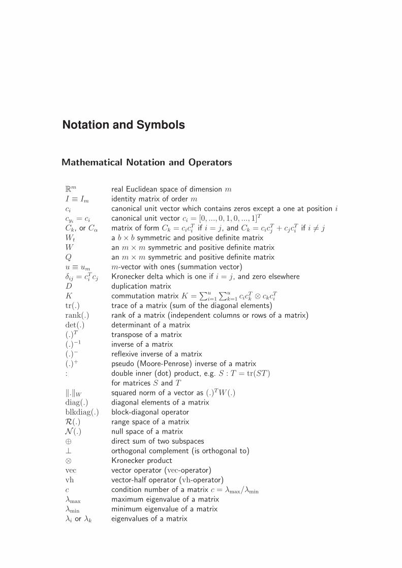
Notation and Symbols
Mathematical Notation and Operators
Rm real Euclidean space of dimension m
I ≡ Im identity matrix of order mci canonical unit vector which contains zeros except a one at position icyi
= ci canonical unit vector ci = [0, ..., 0, 1, 0, ..., 1]T
Ck, or Cα matrix of form Ck = cicTi if i = j, and Ck = cic
Tj + cjc
Ti if i 6= j
Wt a b× b symmetric and positive definite matrixW an m×m symmetric and positive definite matrixQ an m×m symmetric and positive definite matrixu ≡ um m-vector with ones (summation vector)δij = cT
i cj Kronecker delta which is one if i = j, and zero elsewhereD duplication matrixK commutation matrix K =
∑ui=1
∑uk=1 cic
Tk ⊗ ckc
Ti
tr(.) trace of a matrix (sum of the diagonal elements)rank(.) rank of a matrix (independent columns or rows of a matrix)det(.) determinant of a matrix(.)T transpose of a matrix(.)−1 inverse of a matrix(.)− reflexive inverse of a matrix(.)+ pseudo (Moore-Penrose) inverse of a matrix: double inner (dot) product, e.g. S : T = tr(ST )
for matrices S and T‖.‖W squared norm of a vector as (.)T W (.)diag(.) diagonal elements of a matrixblkdiag(.) block-diagonal operatorR(.) range space of a matrixN (.) null space of a matrix⊕ direct sum of two subspaces⊥ orthogonal complement (is orthogonal to)⊗ Kronecker productvec vector operator (vec-operator)vh vector-half operator (vh-operator)c condition number of a matrix c = λmax/λmin
λmax maximum eigenvalue of a matrixλmin minimum eigenvalue of a matrixλi or λk eigenvalues of a matrix
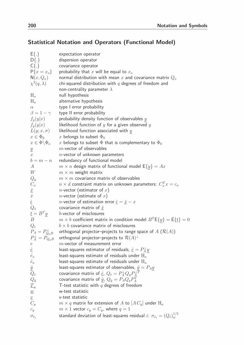
200 Notation and Symbols
Statistical Notation and Operators (Functional Model)
E{.} expectation operatorD{.} dispersion operatorC{.} covariance operatorP{x = xo} probability that x will be equal to xo
N(x,Qx) normal distribution with mean x and covariance matrix Qx
χ2(q, λ) chi-squared distribution with q degrees of freedom andnon-centrality parameter λ
Ho null hypothesisHa alternative hypothesisα type I error probabilityβ = 1− γ type II error probabilityfy(y|x) probability density function of observables yfy(y|x) likelihood function of y for a given observed yL(y; x, σ) likelihood function associated with yx ∈ Φ0 x belongs to subset Φ0
x ∈ Φ\Φo x belongs to subset Φ that is complementary to Φ0
y m-vector of observablesx n-vector of unknown parametersb = m− n redundancy of functional modelA m× n design matrix of functional model E{y} = AxW m×m weight matrixQy m×m covariance matrix of observablesCx n× d constraint matrix on unknown parameters: CT
x x = co
x n-vector (estimator of x)x n-vector (estimate of x)ǫ n-vector of estimation error ǫ = x− xQx covariance matrix of xt = BT y b-vector of misclosuresB m× b coefficient matrix in condition model BT E{y} = E{t} = 0Qt b× b covariance matrix of misclosuresPA = P⊥
QyB orthogonal projector–projects to range space of A (R(A))
P⊥A = PQyB orthogonal projector–projects to R(A)⊥
e m-vector of measurement errore least-squares estimator of residuals, e = P⊥
A yeo least-squares estimate of residuals under Ho
ea least-squares estimate of residuals under Ha
y least-squares estimator of observables, y = PAyQe covariance matrix of e, Qe = P⊥
A QyP⊥TA
Qy covariance matrix of y, Qy = PAQyPTA
T q T-test statistic with q degrees of freedomw w-test statisticv v-test statisticCy m× q matrix for extension of A to [ACy] under Ha
cy m× 1 vector cy = Cy, where q = 1
σeistandard deviation of least-squares residual i: σei
= (Qe)1/2ii
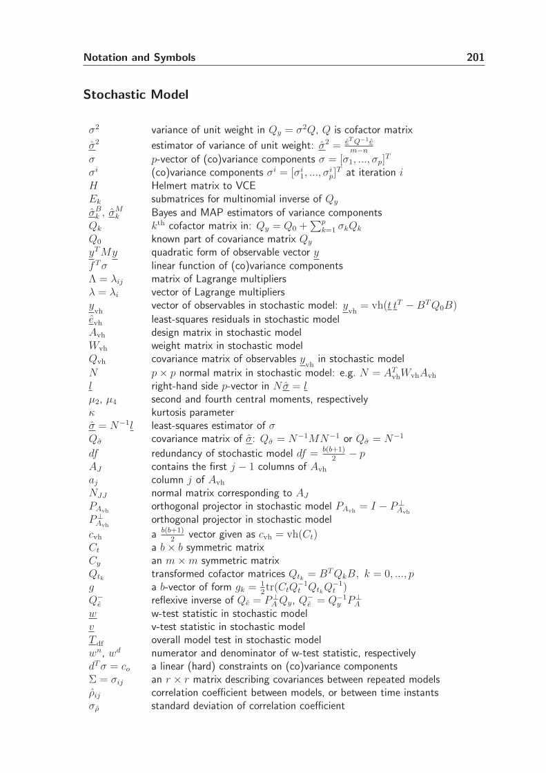
Notation and Symbols 201
Stochastic Model
σ2 variance of unit weight in Qy = σ2Q, Q is cofactor matrix
σ2 estimator of variance of unit weight: σ2 = eT Q−1em−n
σ p-vector of (co)variance components σ = [σ1, ..., σp]T
σi (co)variance components σi = [σi1, ..., σ
ip]
T at iteration iH Helmert matrix to VCEEk submatrices for multinomial inverse of Qy
σBk , σM
k Bayes and MAP estimators of variance componentsQk kth cofactor matrix in: Qy = Q0 +
∑pk=1 σkQk
Q0 known part of covariance matrix Qy
yT My quadratic form of observable vector yfT σ linear function of (co)variance componentsΛ = λij matrix of Lagrange multipliersλ = λi vector of Lagrange multipliersy
vhvector of observables in stochastic model: y
vh= vh(t tT −BT Q0B)
evh least-squares residuals in stochastic modelAvh design matrix in stochastic modelWvh weight matrix in stochastic modelQvh covariance matrix of observables y
vhin stochastic model
N p× p normal matrix in stochastic model: e.g. N = ATvhWvhAvh
l right-hand side p-vector in Nσ = lµ2, µ4 second and fourth central moments, respectivelyκ kurtosis parameterσ = N−1l least-squares estimator of σQσ covariance matrix of σ: Qσ = N−1MN−1 or Qσ = N−1
df redundancy of stochastic model df = b(b+1)2− p
AJ contains the first j − 1 columns of Avh
aj column j of Avh
NJJ normal matrix corresponding to AJ
PAvhorthogonal projector in stochastic model PAvh
= I − P⊥Avh
P⊥Avh
orthogonal projector in stochastic model
cvh a b(b+1)2
vector given as cvh = vh(Ct)Ct a b× b symmetric matrixCy an m×m symmetric matrixQtk transformed cofactor matrices Qtk = BT QkB, k = 0, ..., pg a b-vector of form gk = 1
2tr(CtQ
−1t QtkQ
−1t )
Q−e reflexive inverse of Qe = P⊥
A Qy, Q−e = Q−1
y P⊥A
w w-test statistic in stochastic modelv v-test statistic in stochastic modelT df overall model test in stochastic modelwn, wd numerator and denominator of w-test statistic, respectivelydT σ = co a linear (hard) constraints on (co)variance componentsΣ = σij an r × r matrix describing covariances between repeated modelsρij correlation coefficient between models, or between time instantsσρ standard deviation of correlation coefficient
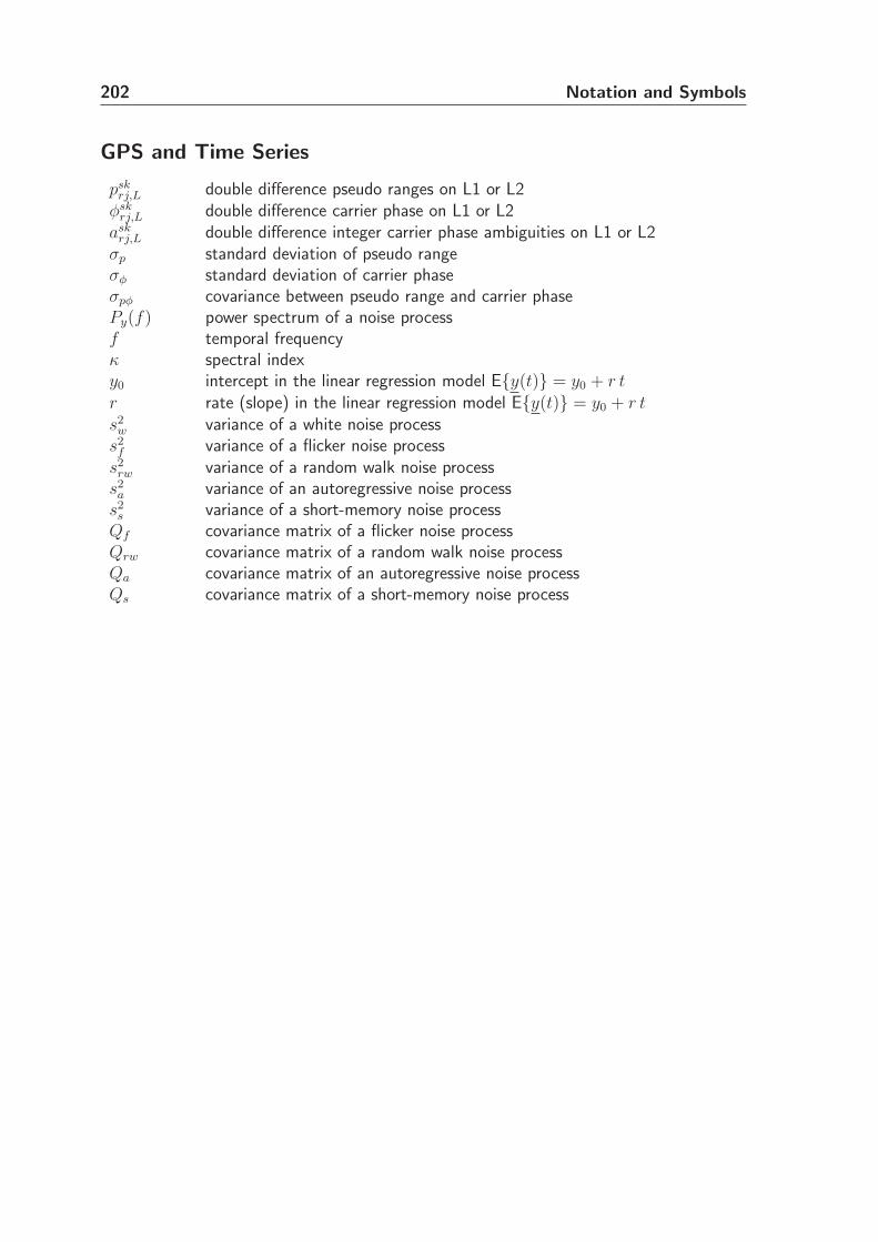
202 Notation and Symbols
GPS and Time Series
pskrj,L double difference pseudo ranges on L1 or L2
φskrj,L double difference carrier phase on L1 or L2
askrj,L double difference integer carrier phase ambiguities on L1 or L2
σp standard deviation of pseudo rangeσφ standard deviation of carrier phaseσpφ covariance between pseudo range and carrier phasePy(f) power spectrum of a noise processf temporal frequencyκ spectral indexy0 intercept in the linear regression model E{y(t)} = y0 + r tr rate (slope) in the linear regression model E{y(t)} = y0 + r ts2
w variance of a white noise processs2
f variance of a flicker noise processs2
rw variance of a random walk noise processs2
a variance of an autoregressive noise processs2
s variance of a short-memory noise processQf covariance matrix of a flicker noise processQrw covariance matrix of a random walk noise processQa covariance matrix of an autoregressive noise processQs covariance matrix of a short-memory noise process
Abstract (in Dutch)
Samenvatting
Gegevensverwerking in geodetische toepassingen vindt doorgaans plaats op basis van dekleinste kwadraten methode. Hiervoor is een goed stochastisch model van de waarnemings-grootheden nodig. Met een dergelijke realistische covariantie-matrix wordt ten eerste debeste (minimum variantie) lineaire zuivere schatter voor de onbekende parameters verkre-gen, en kan ten tweede een realistische precisiebeschrijving van de parameters gegeven wor-den, en kan ten derde, op basis van de verdeling van de waarnemingsgrootheden, hypothesetoetsing correct uitgevoerd worden, en kunnen maten voor kwaliteitscontrole bepaald wor-den, zoals voor betrouwbaarheid. In veel praktische toepassingen is de covariantie-matrixslechts gedeeltelijk bekend. De covariantie-matrix wordt gewoonlijk uitgedrukt als een on-bekende lineaire combinatie van een aantal bekende cofactor matrices. Het schatten vande onbekende (co)variantie componenten wordt in het algemeen variantiecomponenten-schatting (VCS) genoemd, en ook wel kansmodelschatting.
In dit proefschrift bestuderen we de methode van kleinste kwadratenvariantiecomponenten-schatting (KK-VCS) en werken we theoretische en praktischeaspecten uit. We laten zien dat de KK-VCS methode een eenvoudige, flexibele enaantrekkelijke methode is voor VCS. De KK-VCS is eenvoudig, daar ze gebaseerd isop het bekende kleinste kwadraten principe. Met deze methode is de schatting van de(co)variantiecomponenten gebaseerd op een lineair model van waarnemingsvergelijkingen.De methode is flexibel omdat ze werkt met een door de gebruiker gedefinieerde gewichts-matrix. Verschillende klassen van gewichtsmatrices kunnen gedefinieerd worden, dieallemaal automatisch tot zuivere schatters voor de (co)variantie componenten leiden. KK-VCS is aantrekkelijk omdat men de bestaande kleinste kwadraten theorie kan toepassen ophet probleem van variantie-componenten-schatting. Met deze methode kan men 1) matenvoor discrepantie in het stochastisch model verkrijgen, 2) de covariantie-matrix bepalenvan de (co)variantie componenten, 3) de minimum variantie schatter verkrijgen voor de(co)variantie componenten door de inverse van de covariantie-matrix als gewichtsmatrixte nemen, 4) a-priori informatie over de (co)variantie componenten in rekening brengen,5) een niet-lineair (co)variantie componenten model oplossen, 6) robuuste schattingtoepassen op variantie componenten, 7) de schatbaarheid van (co)variantie componentenevalueren, en 8) het probleem van negatieve variantie componenten voorkomen.
Met KK-VCS kunnen vele bestaande VCS methoden, zoals MINQUE, BIQUE, en REMLin een raamwerk geplaatst worden. Deze methoden worden verkregen door speciale keuzesvoor de gewichtsmatrix te maken. Een belangrijke eigenschap van de KK-VCS methodeis de mogelijkheid om hypothese toetsing toe te passen op het stochastisch model. Wegebruiken hiervoor de w-toets, de v-toets, en de globale toets. Ons doel is om een geschikte
204 Abstract (in Dutch)
structuur te vinden voor het stochastisch model, dat alle relevante ruiscomponenten in decovariantie-matrix herbergt. De w-toets wordt geıntroduceerd om te kunnen vaststellenof een bepaalde ruiscomponent met waarschijnlijkheid aanwezig is in de waarnemingen, endientengevolge opgenomen moet worden in het stochastisch model. Gebaseerd op de nor-male verdeling voor oorspronkelijke waarnemingsgrootheden leiden we de verwachting ende variantie van de w-toetsgrootheid af, welke nul en een zijn, respectievelijk. De verdelingis een lineaire combinatie van onderling onafhankelijke centrale chi-kwadraat verdelingen,elk met een vrijheidsgraad. In een aantal speciale gevallen kan deze verdeling benaderdworden door een standaard normale verdeling. Als een equivalente uitdrukking voor dew-toets wordt de v-toetsgrootheid gegeven. Het doel is om het aantal (co)variantie com-ponenten in het stochastisch model te reduceren, door de significantie van de componentente toetsen. De globale toets functioneert als een algemene toets op de geschiktheid vanhet aangenomen stochastisch model.
KK-VCS is toegepast op meetgegevens uit twee GPS toepassingen. Als eerste is demethode toegepast op het GPS geometrievrije model. Daartoe worden het functiemodelen het stochastisch model opgesteld. De variantiecomponenten van verschillende waarne-mingstypen, de satelliet-elevatie afhankelijkheid van de precisie van GPS waarnemingsg-rootheden, en de correlatie tussen verschillende waarnemingstypen worden geschat metKK-VCS. We laten zien dat de precisie van GPS waarnemingsgrootheden duidelijk afhangtvan de elevatie van de satelliet. Ook is er een significante correlatie tussen de waarne-mingstypen. Als tweede toepassing worden de ruiskarakteristieken in tijdreeksen vandagelijkse coordinaten van permanente GPS stations bepaald. De KK-VCS is toegepastom de amplitudes van witte ruis en power-law ruis (flicker ruis en random walk ruis) in dezetijdreeksen te schatten. De resultaten bevestigen dat de tijdreeksen behoorlijk gecorreleerdin de tijd zijn. We hebben ook de w-toetsgrootheid gebruikt om een geschikt stochastischmodel voor de GPS tijdreeksen te vinden. Een combinatie van witte ruis, autoregressieveruis, en flicker ruis karakteriseert in het algemeen de ruis in alle drie positie componentenhet beste. Ongemodelleerde periodieke effecten in de metingen worden beschreven dooreen stel harmonische functies. Deze worden geschat met behulp van de kleinste kwadratenmethode, in hetzelfde raamwerk als KK-VCS. De resultaten bevestigen de aanwezigheidvan jaarlijkse en halfjaarlijkse signalen in de reeksen, als ook andere significante periodiekepatronen. Om onzuivere schatting van de variantiecomponenten te voorkomen, dienendergelijke sinusvormige signalen in het functiemodel opgenomen te worden, alvorens KK-VCS toe te passen.
Curriculum Vitae
AliReza Amiri-Simkooei was born on 24 March 1971 in Bafgh, Yazd, Iran. He graduatedfrom high school in 1989 and, at the same time, he was admitted to the University ofIsfahan, Isfahan, Iran. In Spring 1994 he graduated with high honor–first position–with aBachelor of Science degree in Surveying Engineering. A few months later, he started hismaster study in Geodesy at K.N. Toosi University of Technology, Tehran, Iran. He workedon ‘analytical methods in optimization and design of geodetic networks’ and graduated asan outstanding student in 1998. At the same time he was offered a permanent position atthe University of Isfahan, Isfahan, Iran. He worked there for 4 years mainly lecturing forbachelor students.
In 2002, he was entitled to an overseas PhD scholarship from the Iranian Ministry ofScience, Research and Technology. He worked under supervision of Prof. Peter Teunissenand Dr. Christian Tiberius at the Delft institute of Earth Observation and Space systems(DEOS) of Delft University of Technology, the Netherlands. This thesis covers his PhDstudy. While finalizing his PhD thesis, in late 2006, he started working as a researchassociate at the same institute.
when what where
9.1985 - 6.1989 High school Shariati high school, Kerman
9.1989 - 3.1994 BSc in Surveying The University of Isfahan
9.1994 - 9.1998 MSc in Geodesy K.N. Toosi University of Technology
9.1998 - 9.2002 Lecturer The University of Isfahan
10.2002-4.2007 PhD in Geodesy Delft University of Technology
10.2006- ... Research associate Delft University of Technology

Acknowledgements
This thesis could not be realized without the sincere help and support from many people.It is difficult to thank all the individuals who really need thanking for making this workpossible.
In the first place, I would like to thank my promotor, Prof. Peter Teunissen, for hiscomplete scientific support. I was impressed with his theory on least-squares variancecomponent estimation which was originally developed in 1988. I really enjoyed studyingand elaborating on theoretical and practical aspects of this theory. His valuable suggestionsto improve the early versions of this thesis are gratefully acknowledged.
I would also like to express my deepest thanks to my supervisor, Dr. Christian Tiberius,for his excellent guidances during the last four years working and studying at the Delftinstitute of Earth Observation and Space systems (DEOS) at TU Delft. His open-doorpolicy, accessibility, continuous supervision, quick feedback, friendly behavior and metic-ulous reviewing of the earlier versions of my works along with his valuable comments arekindly appreciated.
I am also very much thankful to all members of the examination committee for theirreviews and useful comments on my thesis.
In this place I would like to thank all of my colleagues at DEOS and specially in MGPfor their support and contribution to a good research environment. A special thanks goesto the following people: Prof. Dick Simons for his help while Prof. Peter Teunissen was onsabbatical in Australia; Dr. Hans van der Marel for his satellite positioning course and hisgeneral support on GPS-related topics; Ria Scholtes for the administrative support; Jaspervan Loon for proofreading this thesis; Peter Joosten for the computer support and for hisMatlab scripts; Dr. Sandra Verhagen for lending me her LATEXstyle file adapted for thisthesis and for her general support; Frans Schroder for helping me make the cover of thethesis; and my former colleague Frank Kenselaar at the start of my PhD research.
I would also like to mention the name of other friends who helped me indirectly tocomplete this work. I can mention at least the names of Dr. Ramon Hanssen, Dr. MirjamSnellen, Dr. Maxim Keshin, Dr. Dennis Odijk, Dr. Frank Kleijer, Dr. Roderik Lindenbergh,Dr. Rossen Grebenitcharsky, Dr. Zbigniew Perski, Anh Quan Le, Yongjin Moon, XianglinLiu, Petar Marinkovic, Benoıt Muth, Junlin Yan, Freek van Leijen, Gini Ketelaar, and Mah-mut Arikan. The best atmosphere creates the best work. I am also indebted to my Iranianfriends Hossein Moosavi Alkazemi, Mohammad Ali Sharifi, Masoud Shirazian, YaghoubHatam Chavari, Saeed Torkzaban, Sirous Ebrahimi, Mahdi Motagh, Hossein Mansouri,Asadollah Shahbahrami, Shohre Shahnoori, Ata Abdollahi Kakroodi, Gholamreza Shams,Ali Heidary, Yahya Memarzadeh, Fatemeh Karimi Nejadasl, and Amir Abbas Zadpoor.
The Iranian Ministry of Science, Research, and Technology as well as Delft University ofTechnology (Department of DEOS) are gratefully acknowledged for their financial supportto pursue my PhD research.

208 Acknowledgements
Finally, I would like to express my sincerest appreciation to my whole family. A sincereappreciation goes to my brothers, sisters and specially to my mother, Fatemeh, whom Ireally missed during this period. I also express my deepest gratitude to my wife and mydaughter, Shahin and Shamim, for their understanding when I was really busy with mywork and for being so patient all those evenings that I was away.