Least-Squares Conditional Density · PDF fileLeast-Squares Conditional Density Estimation 3...

1IEICE Transactions on Information and Systems,vol.E93-D, no.3, pp.583–594, 2010.

Least-Squares Conditional Density Estimation

Masashi Sugiyama ([email protected])Tokyo Institute of Technology

andJapan Science and Technology Agency

Ichiro Takeuchi ([email protected])Nagoya Institute of Technology

Taiji Suzuki ([email protected])The University of Tokyo

Takafumi Kanamori ([email protected])Nagoya University

Hirotaka Hachiya ([email protected])Tokyo Institute of Technology

Daisuke Okanohara ([email protected])The University of Tokyo

Abstract

Estimating the conditional mean of an input-output relation is the goal of regres-sion. However, regression analysis is not sufficiently informative if the conditionaldistribution has multi-modality, is highly asymmetric, or contains heteroscedasticnoise. In such scenarios, estimating the conditional distribution itself would be moreuseful. In this paper, we propose a novel method of conditional density estimationthat is suitable for multi-dimensional continuous variables. The basic idea of theproposed method is to express the conditional density in terms of the density ratioand the ratio is directly estimated without going through density estimation. Ex-periments using benchmark and robot transition datasets illustrate the usefulnessof the proposed approach.

Keywords

Conditional density estimation, multimodality, heteroscedastic noise, direct densityratio estimation, transition estimation

Least-Squares Conditional Density Estimation 2

1 Introduction

Regression is aimed at estimating the conditional mean of output y given input x. Whenthe conditional density p(y|x) is unimodal and symmetric, regression would be sufficientfor analyzing the input-output dependency. However, estimating the conditional meanmay not be sufficiently informative, when the conditional distribution possesses multi-modality (e.g., inverse kinematics learning of a robot [4]) or a highly skewed profile withheteroscedastic noise (e.g., biomedical data analysis [13]). In such cases, it would bemore informative to estimate the conditional distribution itself. In this paper, we addressthe problem of estimating conditional densities when x and y are continuous and multi-dimensional.

When the conditioning variable x is discrete, estimating the conditional densityp(y|x = x) from samples {(xi,yi)}ni=1 is straightforward—by only using samples {yi}ni=1

such that xi = x, a standard density estimation method gives an estimate of the con-ditional density. However, when the conditioning variable x is continuous, conditionaldensity estimation is not straightforward since no sample exactly matches the conditionxi = x. A naive idea for coping with this problem is to use samples {yi}ni=1 that ap-proximately satisfy the condition: xi ≈ x. However, such a naive method is not reliablein high-dimensional problems. Slightly more sophisticated variants have been proposedbased on weighted kernel density estimation [10, 47], but they still share the same weak-ness.

The mixture density network (MDN) [4] models the conditional density by a mixtureof parametric densities, where the parameters are estimated by a neural network. MDNwas shown to work well, although its training is time-consuming and only a local optimalsolution may be obtained due to the non-convexity of neural network learning. Similarly,a mixture of Gaussian processes was explored for estimating the conditional density [42].The mixture model is trained in a computationally efficient manner by an expectation-maximization algorithm [8]. However, since the optimization problem is non-convex, onemay only access to a local optimal solution in practice.

The kernel quantile regression (KQR) method [40, 25] allows one to predict percentilesof the conditional distribution. This implies that solving KQR for all percentiles givesan estimate of the entire conditional cumulative distribution. KQR is formulated as aconvex optimization problem, and therefore a unique global solution can be obtained.Furthermore, the entire solution path with respect to the percentile parameter, whichwas shown to be piece-wise linear, can be computed efficiently [41]. However, the rangeof applications of KQR is limited to one-dimensional output and solution path trackingtends to be numerically rather unstable in practice.

In this paper, we propose a new method of conditional density estimation namedleast-squares conditional density estimation (LS-CDE), which can be applied to multi-dimensional inputs and outputs. The proposed method is based on the fact that theconditional density can be expressed in terms of unconditional densities as p(y|x) =p(x,y)/p(x). Our key idea is that we do not estimate the two densities p(x,y) and p(x)separately, but we directly estimate the density ratio p(x,y)/p(x) without going through


density estimation. Experiments using benchmark and robot transition datasets showthat our method compares favorably with existing methods in terms of the accuracy andcomputational efficiency.

The rest of this paper is organized as follows. In Section 2, we present our proposedmethod LS-CDE and investigate its theoretical properties. In Section 3, we discuss thecharacteristics of existing and proposed approaches. In Section 4, we compare the ex-perimental performance of the proposed and existing methods. Finally, in Section 5, weconclude by summarizing our contributions and outlook.

2 A New Method of Conditional Density Estimation

In this section, we formulate the problem of conditional density estimation and give anew method.

2.1 Conditional Density Estimation via Density Ratio Estima-tion

Let DX (⊂ RdX) and DY (⊂ RdY) be input and output data domains, where dX and dY arethe dimensionality of the data domains, respectively. Let us consider a joint probabilitydistribution on DX ×DY with probability density function p(x,y), and suppose that weare given n independent and identically distributed (i.i.d.) paired samples of input x andoutput y:

{zi | zi = (xi,yi) ∈ DX ×DY}ni=1.

The goal is to estimate the conditional density p(y|x) from the samples {zi}ni=1.Our primal interest is in the case where both variables x and y are continuous. In

this case, conditional density estimation is not straightforward since no sample exactlymatches the condition.

Our proposed approach is to consider the ratio of two densities:

p(y|x) = p(x,y)

p(x):= r(x,y),

where we assume p(x) > 0 for all x ∈ DX. However, naively estimating two densitiesand taking their ratio can result in large estimation error. In order to avoid this, wepropose to estimate the density ratio function r(x,y) directly without going throughdensity estimation of p(x,y) and p(x).

2.2 Linear Density-ratio Model

We model the density ratio function r(x,y) by the following linear model:

rα(x,y) := α⊤ϕ(x,y), (1)


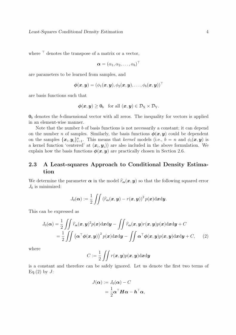
where ⊤ denotes the transpose of a matrix or a vector,

α = (α1, α2, . . . , αb)⊤

are parameters to be learned from samples, and

ϕ(x,y) = (ϕ1(x,y), ϕ2(x,y), . . . , ϕb(x,y))⊤

are basis functions such that

ϕ(x,y) ≥ 0b for all (x,y) ∈ DX ×DY.

0b denotes the b-dimensional vector with all zeros. The inequality for vectors is appliedin an element-wise manner.

Note that the number b of basis functions is not necessarily a constant; it can dependon the number n of samples. Similarly, the basis functions ϕ(x,y) could be dependenton the samples {xi,yi}ni=1. This means that kernel models (i.e., b = n and ϕi(x,y) isa kernel function ‘centered’ at (xi,yi)) are also included in the above formulation. Weexplain how the basis functions ϕ(x,y) are practically chosen in Section 2.6.

2.3 A Least-squares Approach to Conditional Density Estima-tion

We determine the parameter α in the model rα(x,y) so that the following squared errorJ0 is minimized:

J0(α) :=1

2

∫∫(rα(x,y)− r(x,y))2 p(x)dxdy.

This can be expressed as

J0(α) =1

2

∫∫rα(x,y)

2p(x)dxdy −∫∫

rα(x,y)r(x,y)p(x)dxdy + C

=1

2

∫∫ (α⊤ϕ(x,y)

)2p(x)dxdy −

∫∫α⊤ϕ(x,y)p(x,y)dxdy + C, (2)

where

C :=1

2

∫∫r(x,y)p(x,y)dxdy

is a constant and therefore can be safely ignored. Let us denote the first two terms ofEq.(2) by J :

J(α) := J0(α)− C

=1

2α⊤Hα− h⊤α,


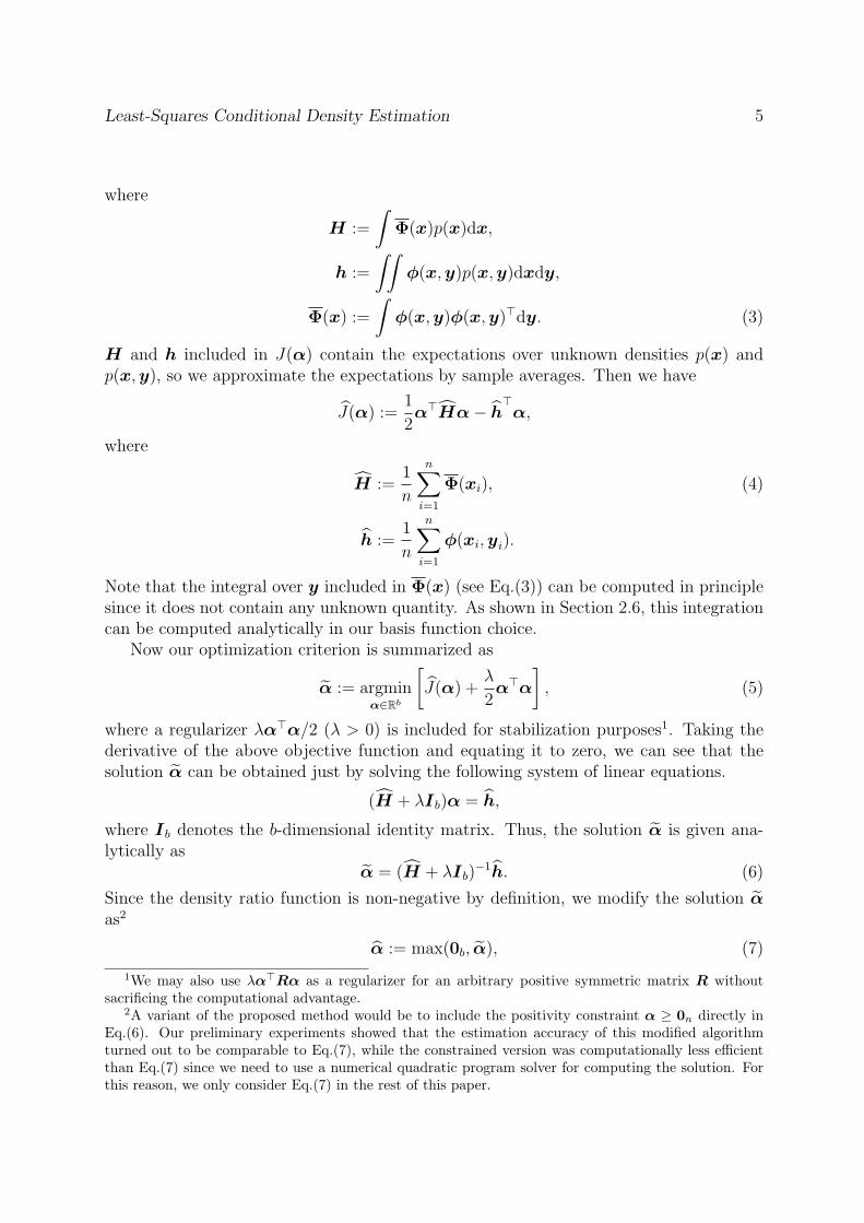
where

H :=

∫Φ(x)p(x)dx,

h :=

∫∫ϕ(x,y)p(x,y)dxdy,

Φ(x) :=

∫ϕ(x,y)ϕ(x,y)⊤dy. (3)

H and h included in J(α) contain the expectations over unknown densities p(x) andp(x,y), so we approximate the expectations by sample averages. Then we have

J(α) :=1

2α⊤Hα− h

⊤α,

where

H :=1

n

n∑i=1

Φ(xi), (4)

h :=1

n

n∑i=1

ϕ(xi,yi).

Note that the integral over y included in Φ(x) (see Eq.(3)) can be computed in principlesince it does not contain any unknown quantity. As shown in Section 2.6, this integrationcan be computed analytically in our basis function choice.

Now our optimization criterion is summarized as

α := argminα∈Rb

[J(α) +

λ

2α⊤α

], (5)

where a regularizer λα⊤α/2 (λ > 0) is included for stabilization purposes1. Taking thederivative of the above objective function and equating it to zero, we can see that thesolution α can be obtained just by solving the following system of linear equations.

(H + λIb)α = h,

where Ib denotes the b-dimensional identity matrix. Thus, the solution α is given ana-lytically as

α = (H + λIb)−1h. (6)

Since the density ratio function is non-negative by definition, we modify the solution αas2

α := max(0b, α), (7)

1We may also use λα⊤Rα as a regularizer for an arbitrary positive symmetric matrix R withoutsacrificing the computational advantage.

2A variant of the proposed method would be to include the positivity constraint α ≥ 0n directly inEq.(6). Our preliminary experiments showed that the estimation accuracy of this modified algorithmturned out to be comparable to Eq.(7), while the constrained version was computationally less efficientthan Eq.(7) since we need to use a numerical quadratic program solver for computing the solution. Forthis reason, we only consider Eq.(7) in the rest of this paper.


where the ‘max’ operation for vectors is applied in an element-wise manner. Thanksto this rounding-up processing, the solution α tends to be sparse, which contributes toreducing the computation time in the test phase.

In order to assure that the obtained density-ratio function is a conditional density, werenormalize the solution in the test phase—given a test input point x, our final solutionis given as

p(y|x = x) =α⊤ϕ(x,y)∫α⊤ϕ(x,y′)dy′

. (8)

We call the above method Least-Squares Conditional Density Estimation (LS-CDE). LS-CDE can be regarded as an application of the direct density ratio estimation method calledthe unconstrained Least-Squares Importance Fitting (uLSIF) [17, 18] to the problem ofdensity ratio estimation.

A MATLAB R⃝ implementation of the LS-CDE algorithm is available from

http://sugiyama-www.cs.titech.ac.jp/~sugi/software/LSCDE/

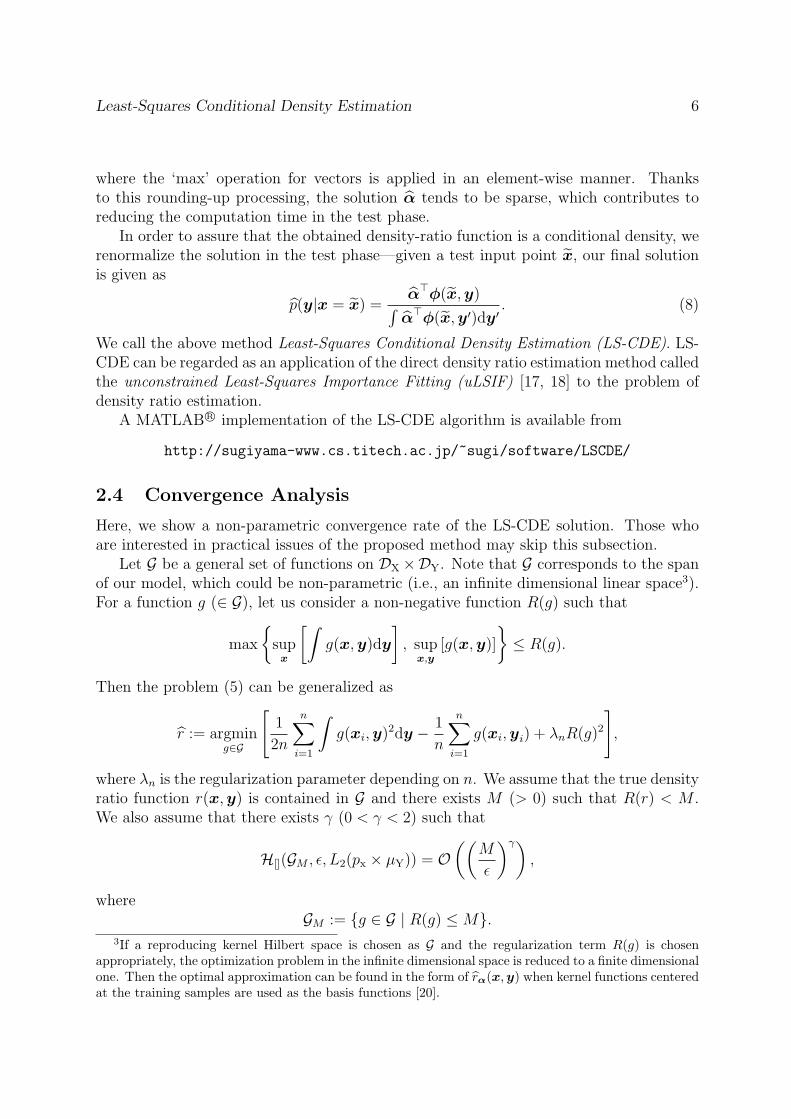
2.4 Convergence Analysis

Here, we show a non-parametric convergence rate of the LS-CDE solution. Those whoare interested in practical issues of the proposed method may skip this subsection.

Let G be a general set of functions on DX ×DY. Note that G corresponds to the spanof our model, which could be non-parametric (i.e., an infinite dimensional linear space3).For a function g (∈ G), let us consider a non-negative function R(g) such that

max

{supx

[∫g(x,y)dy

], sup

x,y[g(x,y)]

}≤ R(g).

Then the problem (5) can be generalized as

r := argming∈G

[1

2n

n∑i=1

∫g(xi,y)

2dy − 1

n

n∑i=1

g(xi,yi) + λnR(g)2

],

where λn is the regularization parameter depending on n. We assume that the true densityratio function r(x,y) is contained in G and there exists M (> 0) such that R(r) < M .We also assume that there exists γ (0 < γ < 2) such that

H[](GM , ϵ, L2(px × µY)) = O((

M

ϵ

)γ),

whereGM := {g ∈ G | R(g) ≤M}.

3If a reproducing kernel Hilbert space is chosen as G and the regularization term R(g) is chosenappropriately, the optimization problem in the infinite dimensional space is reduced to a finite dimensionalone. Then the optimal approximation can be found in the form of rα(x,y) when kernel functions centeredat the training samples are used as the basis functions [20].


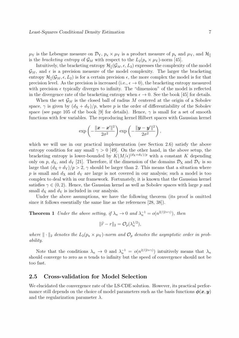
µY is the Lebesgue measure on DY, px × µY is a product measure of px and µY, and H[]

is the bracketing entropy of GM with respect to the L2(px × µY)-norm [45].Intuitively, the bracketing entropyH[](GM , ϵ, L2) expresses the complexity of the model

GM , and ϵ is a precision measure of the model complexity. The larger the bracketingentropy H[](GM , ϵ, L2) is for a certain precision ϵ, the more complex the model is for thatprecision level. As the precision is increased (i.e., ϵ→ 0), the bracketing entropy measuredwith precision ϵ typically diverges to infinity. The “dimension” of the model is reflectedin the divergence rate of the bracketing entropy when ϵ→ 0. See the book [45] for details.

When the set GM is the closed ball of radius M centered at the origin of a Sobolevspace, γ is given by (dX + dY)/p, where p is the order of differentiability of the Sobolevspace (see page 105 of the book [9] for details). Hence, γ is small for a set of smoothfunctions with few variables. The reproducing kernel Hilbert spaces with Gaussian kernel

exp

(−∥x− x′∥2

2σ2

)exp

(−∥y − y′∥2

2σ2

),

which we will use in our practical implementation (see Section 2.6) satisfy the aboveentropy condition for any small γ > 0 [49]. On the other hand, in the above setup, thebracketing entropy is lower-bounded by K(M/ϵ)(dX+dY)/p with a constant K dependingonly on p, dX, and dY [21]. Therefore, if the dimension of the domains DX and DY is solarge that (dX + dY)/p > 2, γ should be larger than 2. This means that a situation wherep is small and dX and dY are large is not covered in our analysis; such a model is toocomplex to deal with in our framework. Fortunately, it is known that the Gaussian kernelsatisfies γ ∈ (0, 2). Hence, the Gaussian kernel as well as Sobolev spaces with large p andsmall dX and dY is included in our analysis.

Under the above assumptions, we have the following theorem (its proof is omittedsince it follows essentially the same line as the references [28, 38]).

Theorem 1 Under the above setting, if λn → 0 and λ−1n = o(n2/(2+γ)), then

∥r − r∥2 = Op(λ1/2n ),

where ∥ · ∥2 denotes the L2(px × µY)-norm and Op denotes the asymptotic order in prob-ability.

Note that the conditions λn → 0 and λ−1n = o(n2/(2+γ)) intuitively means that λn

should converge to zero as n tends to infinity but the speed of convergence should not betoo fast.

2.5 Cross-validation for Model Selection

We elucidated the convergence rate of the LS-CDE solution. However, its practical perfor-mance still depends on the choice of model parameters such as the basis functions ϕ(x,y)and the regularization parameter λ.


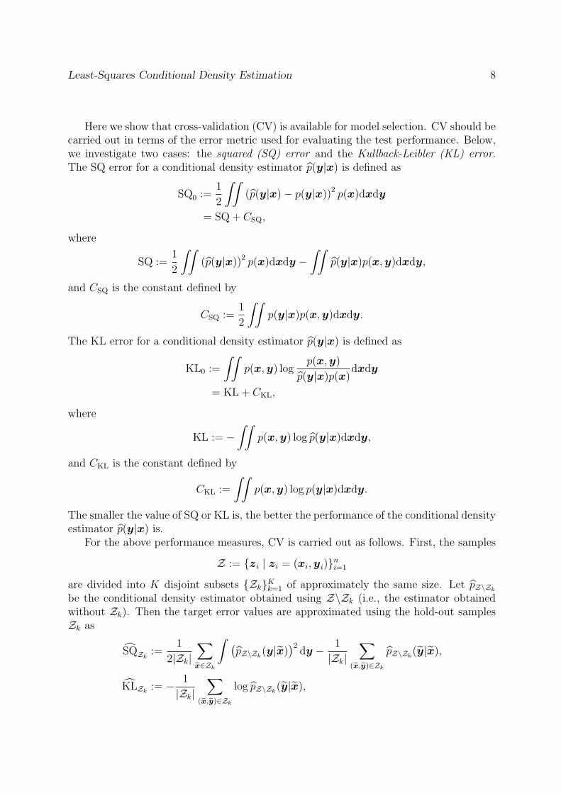
Here we show that cross-validation (CV) is available for model selection. CV should becarried out in terms of the error metric used for evaluating the test performance. Below,we investigate two cases: the squared (SQ) error and the Kullback-Leibler (KL) error.The SQ error for a conditional density estimator p(y|x) is defined as

SQ0 :=1

2

∫∫(p(y|x)− p(y|x))2 p(x)dxdy

= SQ + CSQ,

where

SQ :=1

2

∫∫(p(y|x))2 p(x)dxdy −

∫∫p(y|x)p(x,y)dxdy,

and CSQ is the constant defined by

CSQ :=1

2

∫∫p(y|x)p(x,y)dxdy.

The KL error for a conditional density estimator p(y|x) is defined as

KL0 :=

∫∫p(x,y) log

p(x,y)

p(y|x)p(x)dxdy

= KL + CKL,

where

KL := −∫∫

p(x,y) log p(y|x)dxdy,

and CKL is the constant defined by

CKL :=

∫∫p(x,y) log p(y|x)dxdy.

The smaller the value of SQ or KL is, the better the performance of the conditional densityestimator p(y|x) is.

For the above performance measures, CV is carried out as follows. First, the samples

Z := {zi | zi = (xi,yi)}ni=1

are divided into K disjoint subsets {Zk}Kk=1 of approximately the same size. Let pZ\Zk

be the conditional density estimator obtained using Z\Zk (i.e., the estimator obtainedwithout Zk). Then the target error values are approximated using the hold-out samplesZk as

SQZk:=

1

2|Zk|∑x∈Zk

∫ (pZ\Zk

(y|x))2

dy − 1

|Zk|∑

(x,y)∈Zk

pZ\Zk(y|x),

KLZk:= − 1

|Zk|∑

(x,y)∈Zk

log pZ\Zk(y|x),


where |Zk| denotes the number of elements in the set Zk. This procedure is repeated fork = 1, 2, . . . , K and its average is computed:

SQ :=1

K

K∑k=1

SQZk,

KL :=1

K

K∑k=1

KLZk.

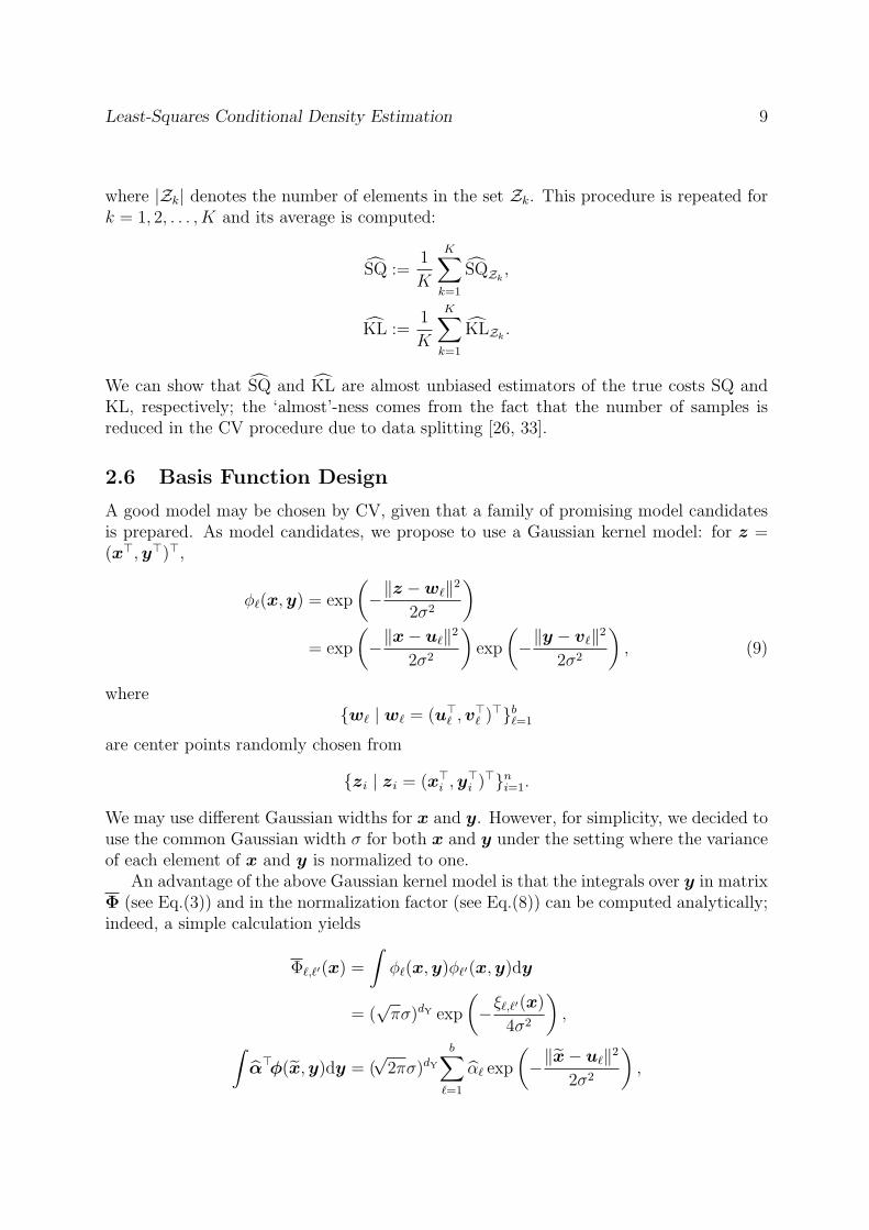
We can show that SQ and KL are almost unbiased estimators of the true costs SQ andKL, respectively; the ‘almost’-ness comes from the fact that the number of samples isreduced in the CV procedure due to data splitting [26, 33].

2.6 Basis Function Design

A good model may be chosen by CV, given that a family of promising model candidatesis prepared. As model candidates, we propose to use a Gaussian kernel model: for z =(x⊤,y⊤)⊤,

ϕℓ(x,y) = exp

(−∥z −wℓ∥2

2σ2

)= exp

(−∥x− uℓ∥2

2σ2

)exp

(−∥y − vℓ∥2

2σ2

), (9)

where{wℓ | wℓ = (u⊤

ℓ ,v⊤ℓ )

⊤}bℓ=1

are center points randomly chosen from

{zi | zi = (x⊤i ,y

⊤i )

⊤}ni=1.

We may use different Gaussian widths for x and y. However, for simplicity, we decided touse the common Gaussian width σ for both x and y under the setting where the varianceof each element of x and y is normalized to one.

An advantage of the above Gaussian kernel model is that the integrals over y in matrixΦ (see Eq.(3)) and in the normalization factor (see Eq.(8)) can be computed analytically;indeed, a simple calculation yields

Φℓ,ℓ′(x) =

∫ϕℓ(x,y)ϕℓ′(x,y)dy

= (√πσ)dY exp

(−ξℓ,ℓ

′(x)

4σ2

),∫

α⊤ϕ(x,y)dy = (√2πσ)dY

b∑ℓ=1

αℓ exp

(−∥x− uℓ∥2

2σ2

),


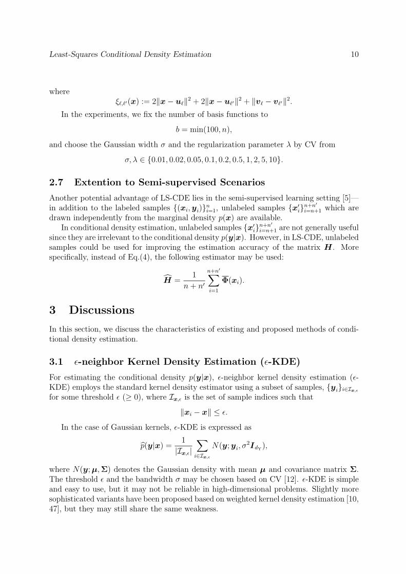
whereξℓ,ℓ′(x) := 2∥x− uℓ∥2 + 2∥x− uℓ′∥2 + ∥vℓ − vℓ′∥2.

In the experiments, we fix the number of basis functions to

b = min(100, n),

and choose the Gaussian width σ and the regularization parameter λ by CV from

σ, λ ∈ {0.01, 0.02, 0.05, 0.1, 0.2, 0.5, 1, 2, 5, 10}.

2.7 Extention to Semi-supervised Scenarios

Another potential advantage of LS-CDE lies in the semi-supervised learning setting [5]—in addition to the labeled samples {(xi,yi)}ni=1, unlabeled samples {x′

i}n+n′

i=n+1 which aredrawn independently from the marginal density p(x) are available.

In conditional density estimation, unlabeled samples {x′i}n+n′

i=n+1 are not generally usefulsince they are irrelevant to the conditional density p(y|x). However, in LS-CDE, unlabeledsamples could be used for improving the estimation accuracy of the matrix H . Morespecifically, instead of Eq.(4), the following estimator may be used:

H =1

n+ n′

n+n′∑i=1

Φ(xi).

3 Discussions

In this section, we discuss the characteristics of existing and proposed methods of condi-tional density estimation.

3.1 ϵ-neighbor Kernel Density Estimation (ϵ-KDE)

For estimating the conditional density p(y|x), ϵ-neighbor kernel density estimation (ϵ-KDE) employs the standard kernel density estimator using a subset of samples, {yi}i∈Ix,ϵ

for some threshold ϵ (≥ 0), where Ix,ϵ is the set of sample indices such that

∥xi − x∥ ≤ ϵ.

In the case of Gaussian kernels, ϵ-KDE is expressed as

p(y|x) = 1

|Ix,ϵ|∑i∈Ix,ϵ

N(y;yi, σ2IdY),

where N(y;µ,Σ) denotes the Gaussian density with mean µ and covariance matrix Σ.The threshold ϵ and the bandwidth σ may be chosen based on CV [12]. ϵ-KDE is simpleand easy to use, but it may not be reliable in high-dimensional problems. Slightly moresophisticated variants have been proposed based on weighted kernel density estimation [10,47], but they may still share the same weakness.


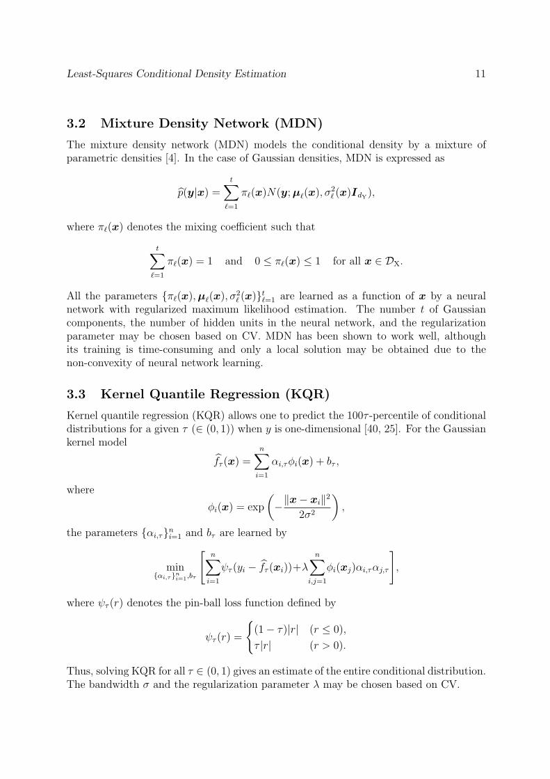
3.2 Mixture Density Network (MDN)

The mixture density network (MDN) models the conditional density by a mixture ofparametric densities [4]. In the case of Gaussian densities, MDN is expressed as

p(y|x) =t∑

ℓ=1

πℓ(x)N(y;µℓ(x), σ2ℓ (x)IdY),

where πℓ(x) denotes the mixing coefficient such that

t∑ℓ=1

πℓ(x) = 1 and 0 ≤ πℓ(x) ≤ 1 for all x ∈ DX.

All the parameters {πℓ(x),µℓ(x), σ2ℓ (x)}tℓ=1 are learned as a function of x by a neural

network with regularized maximum likelihood estimation. The number t of Gaussiancomponents, the number of hidden units in the neural network, and the regularizationparameter may be chosen based on CV. MDN has been shown to work well, althoughits training is time-consuming and only a local solution may be obtained due to thenon-convexity of neural network learning.

3.3 Kernel Quantile Regression (KQR)

Kernel quantile regression (KQR) allows one to predict the 100τ -percentile of conditionaldistributions for a given τ (∈ (0, 1)) when y is one-dimensional [40, 25]. For the Gaussiankernel model

fτ (x) =n∑

i=1

αi,τϕi(x) + bτ ,

where

ϕi(x) = exp

(−∥x− xi∥2

2σ2

),

the parameters {αi,τ}ni=1 and bτ are learned by

min{αi,τ}ni=1,bτ

[n∑

i=1

ψτ (yi − fτ (xi))+λn∑

i,j=1

ϕi(xj)αi,ταj,τ

],

where ψτ (r) denotes the pin-ball loss function defined by

ψτ (r) =

{(1− τ)|r| (r ≤ 0),

τ |r| (r > 0).

Thus, solving KQR for all τ ∈ (0, 1) gives an estimate of the entire conditional distribution.The bandwidth σ and the regularization parameter λ may be chosen based on CV.


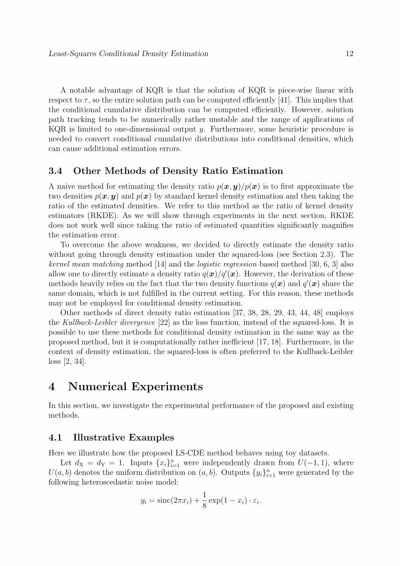
A notable advantage of KQR is that the solution of KQR is piece-wise linear withrespect to τ , so the entire solution path can be computed efficiently [41]. This implies thatthe conditional cumulative distribution can be computed efficiently. However, solutionpath tracking tends to be numerically rather unstable and the range of applications ofKQR is limited to one-dimensional output y. Furthermore, some heuristic procedure isneeded to convert conditional cumulative distributions into conditional densities, whichcan cause additional estimation errors.

3.4 Other Methods of Density Ratio Estimation

A naive method for estimating the density ratio p(x,y)/p(x) is to first approximate thetwo densities p(x,y) and p(x) by standard kernel density estimation and then taking theratio of the estimated densities. We refer to this method as the ratio of kernel densityestimators (RKDE). As we will show through experiments in the next section, RKDEdoes not work well since taking the ratio of estimated quantities significantly magnifiesthe estimation error.

To overcome the above weakness, we decided to directly estimate the density ratiowithout going through density estimation under the squared-loss (see Section 2.3). Thekernel mean matching method [14] and the logistic regression based method [30, 6, 3] alsoallow one to directly estimate a density ratio q(x)/q′(x). However, the derivation of thesemethods heavily relies on the fact that the two density functions q(x) and q′(x) share thesame domain, which is not fulfilled in the current setting. For this reason, these methodsmay not be employed for conditional density estimation.

Other methods of direct density ratio estimation [37, 38, 28, 29, 43, 44, 48] employsthe Kullback-Leibler divergence [22] as the loss function, instead of the squared-loss. It ispossible to use these methods for conditional density estimation in the same way as theproposed method, but it is computationally rather inefficient [17, 18]. Furthermore, in thecontext of density estimation, the squared-loss is often preferred to the Kullback-Leiblerloss [2, 34].

4 Numerical Experiments

In this section, we investigate the experimental performance of the proposed and existingmethods.

4.1 Illustrative Examples

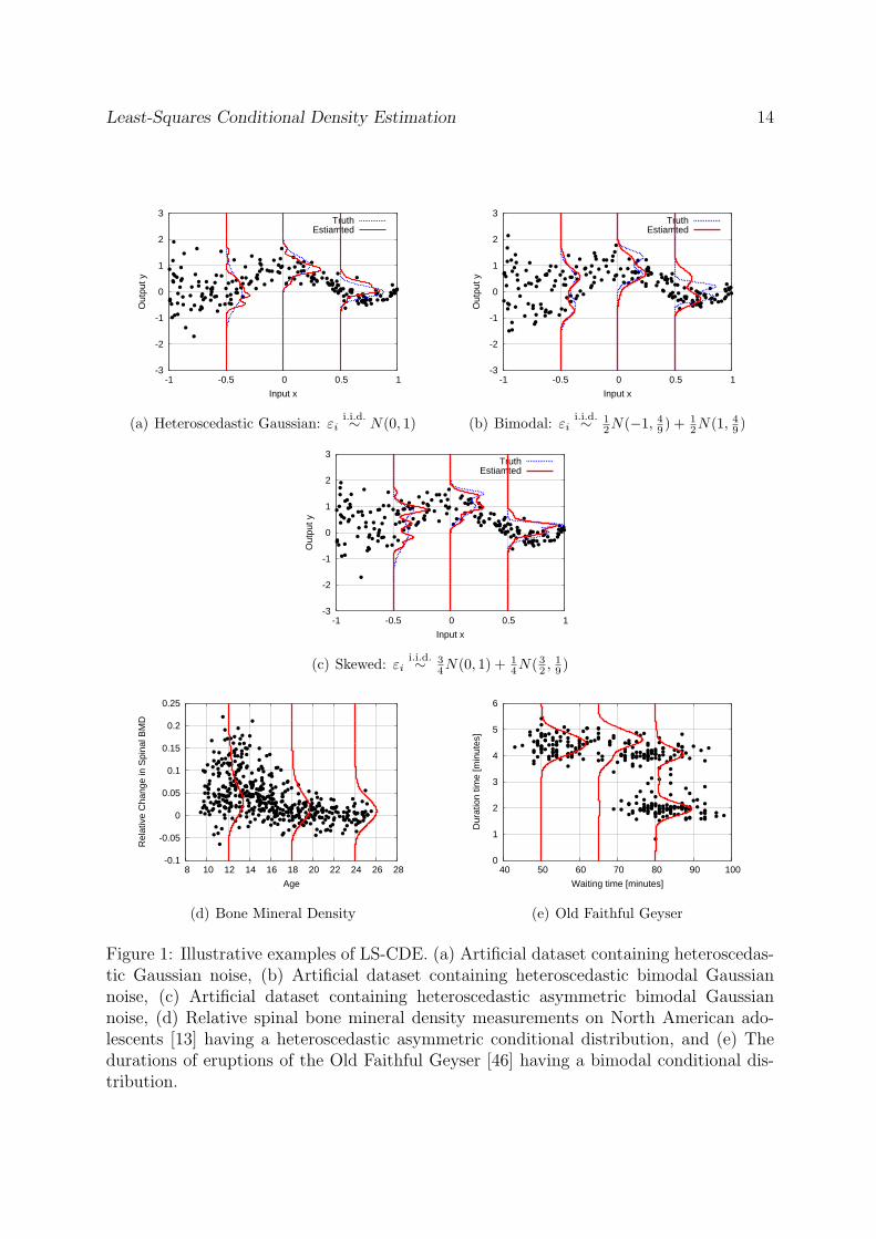
Here we illustrate how the proposed LS-CDE method behaves using toy datasets.Let dX = dY = 1. Inputs {xi}ni=1 were independently drawn from U(−1, 1), where

U(a, b) denotes the uniform distribution on (a, b). Outputs {yi}ni=1 were generated by thefollowing heteroscedastic noise model:

yi = sinc(2πxi) +1

8exp(1− xi) · εi.


We tested the following three different distributions for {εi}ni=1:

(a) Gaussian: εii.i.d.∼ N(0, 1),

(b) Bimodal: εii.i.d.∼ 1

2N(−1, 4

9) + 1

2N(1, 4

9),

(c) Skewed: εii.i.d.∼ 3

4N(0, 1) + 1

4N(3

2, 19),

where ‘i.i.d.∼ ’ denotes ‘independent and identically distributed’ and N(µ, σ2) denotes the

Gaussian distribution with mean µ and variance σ2. See Figure 1(a)–Figure 1(c) fortheir profiles. The number of training samples was set to n = 200. The numericalresults were depicted in Figure 1(a)–Figure 1(c), illustrating that LS-CDE well capturesheteroscedasticity, bimodality, and asymmetricity.

We have also investigated the experimental performance of LS-CDE using the followingreal datasets:

(d) Bone Mineral Density dataset: Relative spinal bone mineral density measure-ments on 485 North American adolescents [13], having a heteroscedastic asymmetricconditional distribution.

(e) Old Faithful Geyser dataset: The durations of 299 eruptions of the Old FaithfulGeyser [46], having a bimodal conditional distribution.

Figure 1(d) and Figure 1(e) depict the results, showing that heteroscedastic and multi-modal structures were nicely revealed by LS-CDE.

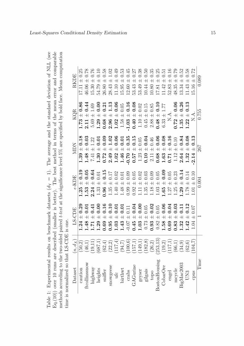
4.2 Benchmark Datasets

We applied the proposed and existing methods to the benchmark datasets accompaniedwith the R package [31] (see Table 1) and evaluate their experimental performance.

In each dataset, 50% of samples were randomly chosen for conditional density esti-mation and the rest was used for computing the estimation accuracy. The accuracy of aconditional density estimator p(y|x) was measured by the negative log-likelihood for testsamples {zi | zi = (xi, yi)}ni=1:

NLL := − 1

n

n∑i=1

log p(yi|xi). (10)

Thus, the smaller the value of NLL is, the better the performance of the conditionaldensity estimator p(y|x) is.


-3

-2

-1

0

1

2

3

-1 -0.5 0 0.5 1

Out

put y

Input x

TruthEstiamted

(a) Heteroscedastic Gaussian: εii.i.d.∼ N(0, 1)

-3

-2

-1

0

1

2

3

-1 -0.5 0 0.5 1

Out

put y

Input x

TruthEstiamted

(b) Bimodal: εii.i.d.∼ 1

2N(−1, 49 ) +

12N(1, 4

9 )

-3

-2

-1

0

1

2

3

-1 -0.5 0 0.5 1

Out

put y

Input x

TruthEstiamted

(c) Skewed: εii.i.d.∼ 3

4N(0, 1) + 14N( 32 ,

19 )

-0.1

-0.05

0

0.05

0.1

0.15

0.2

0.25

8 10 12 14 16 18 20 22 24 26 28

Rel

ativ

e C

hang

e in

Spi

nal B

MD

Age

(d) Bone Mineral Density

0

1

2

3

4

5

6

40 50 60 70 80 90 100

Dur

atio

n tim

e [m

inut

es]

Waiting time [minutes]

(e) Old Faithful Geyser

Figure 1: Illustrative examples of LS-CDE. (a) Artificial dataset containing heteroscedas-tic Gaussian noise, (b) Artificial dataset containing heteroscedastic bimodal Gaussiannoise, (c) Artificial dataset containing heteroscedastic asymmetric bimodal Gaussiannoise, (d) Relative spinal bone mineral density measurements on North American ado-lescents [13] having a heteroscedastic asymmetric conditional distribution, and (e) Thedurations of eruptions of the Old Faithful Geyser [46] having a bimodal conditional dis-tribution.


Tab

le1:

Experim

entalresultson

benchmarkdatasets(d

Y=

1).Theaveragean

dthestan

darddeviation

ofNLL

(see

Eq.(10))

over

10runsaredescribed

(smalleris

better).

Thebestmethodin

term

sof

themeanerroran

dcomparab

lemethodsaccordingto

thetw

o-sided

pairedt-test

atthesign

ificance

level5%

arespecified

byboldface.Meancomputation

timeisnormalized

sothat

LS-C

DEison

e.

Dataset

(n,d

X)

LS-C

DE

ϵ-KDE

MDN

KQR

RKDE

caution

(50,2)

1.24±

0.29

1.25±

0.19

1.39±

0.18

1.73±

0.86

17.11±

0.25

ftcollinssnow

(46,1)

1.48±

0.01

1.53±

0.05

1.48±

0.03

2.11±

0.44

46.06±

0.78

highway

(19,11)

1.71±

0.41

2.24±

0.64

7.41

±1.22

5.69

±1.69

15.30±

0.76

heigh

ts(687,1)

1.29±

0.00

1.33

±0.01

1.30±

0.01

1.29±

0.00

54.79±

0.10

sniffer

(62,4)

0.69±

0.16

0.96±

0.15

0.72±

0.09

0.68±

0.21

26.80±

0.58

snow

geese

(22,2)

0.95±

0.10

1.35

±0.17

2.49±

1.02

2.96±

1.13

28.43±

1.02

ufc

(117,4)

1.03±

0.01

1.40

±0.02

1.02±

0.06

1.02±

0.06

11.10±

0.49

birthwt

(94,7)

1.43±

0.01

1.48

±0.01

1.46±

0.01

1.58

±0.05

15.95±

0.53

crab

s(100,6)

-0.07±

0.11

0.99

±0.09

-0.70±

0.35

-1.03±

0.16

12.60±

0.45

GAGurine

(157,1)

0.45±

0.04

0.92

±0.05

0.57±

0.15

0.40±

0.08

53.43±

0.27

geyser

(149,1)

1.03±

0.00

1.11

±0.02

1.23

±0.05

1.10

±0.02

53.49±

0.38

gilgais

(182,8)

0.73

±0.05

1.35

±0.03

0.10±

0.04

0.45

±0.15

10.44±

0.50

topo

(26,2)

0.93±

0.02

1.18

±0.09

2.11

±0.46

2.88

±0.85

10.80±

0.35

BostonHou

sing

(253,13)

0.82

±0.05

1.03

±0.05

0.68±

0.06

0.48±

0.10

17.81±

0.25

Cob

arOre

(19,2)

1.58±

0.06

1.65±

0.09

1.63±

0.08

6.33

±1.77

11.42±

0.51

engel

(117,1)

0.69±

0.04

1.27

±0.05

0.71±

0.16

N.A

.52.83±

0.16

mcycle

(66,1)

0.83±

0.03

1.25

±0.23

1.12

±0.10

0.72±

0.06

48.35±

0.79

BigMac2003

(34,9)

1.32±

0.11

1.29±

0.14

2.64±

0.84

1.35±

0.26

13.34±

0.52

UN3

(62,6)

1.42±

0.12

1.78

±0.14

1.32±

0.08

1.22±

0.13

11.43±

0.58

cpus

(104,7)

1.04

±0.07

1.01

±0.10

-2.14±

0.13

N.A

.15.16±

0.72

Tim

e1

0.004

267

0.755

0.089


We compared LS-CDE, ϵ-KDE, MDN, KQR, and RKDE. For model selection, weused CV based on the Kullback-Leibler (KL) error (see Section 2.5), which is consistentwith the above NLL. In MDN, CV over three tuning parameters (the number of Gaussiancomponents, the number of hidden units in the neural network, and the regularizationparameter; see Section 3.2) was unbearably slow, so the number of Gaussian componentswas fixed to t = 3 and the other two tuning parameters were chosen by CV.

The experimental results are summarized in Table 1. ϵ-KDE was computationallyvery efficient, but it tended to perform rather poorly. MDN worked well, but it is com-putationally highly demanding. KQR overall performed well and it was computationallyslightly more efficient than LS-CDE. However, its solution path tracking algorithm wasnumerically rather unstable and we could not obtain solutions for the ‘engel’ and ‘cpus’datasets. RKDE did not perform well for all cases, implying that density ratio estima-tion via density estimation is not reliable in practice. Overall, the proposed LS-CDEwas shown to be a promising method for conditional density estimation in terms of theaccuracy and computational efficiency.

4.3 Robot Transition Estimation

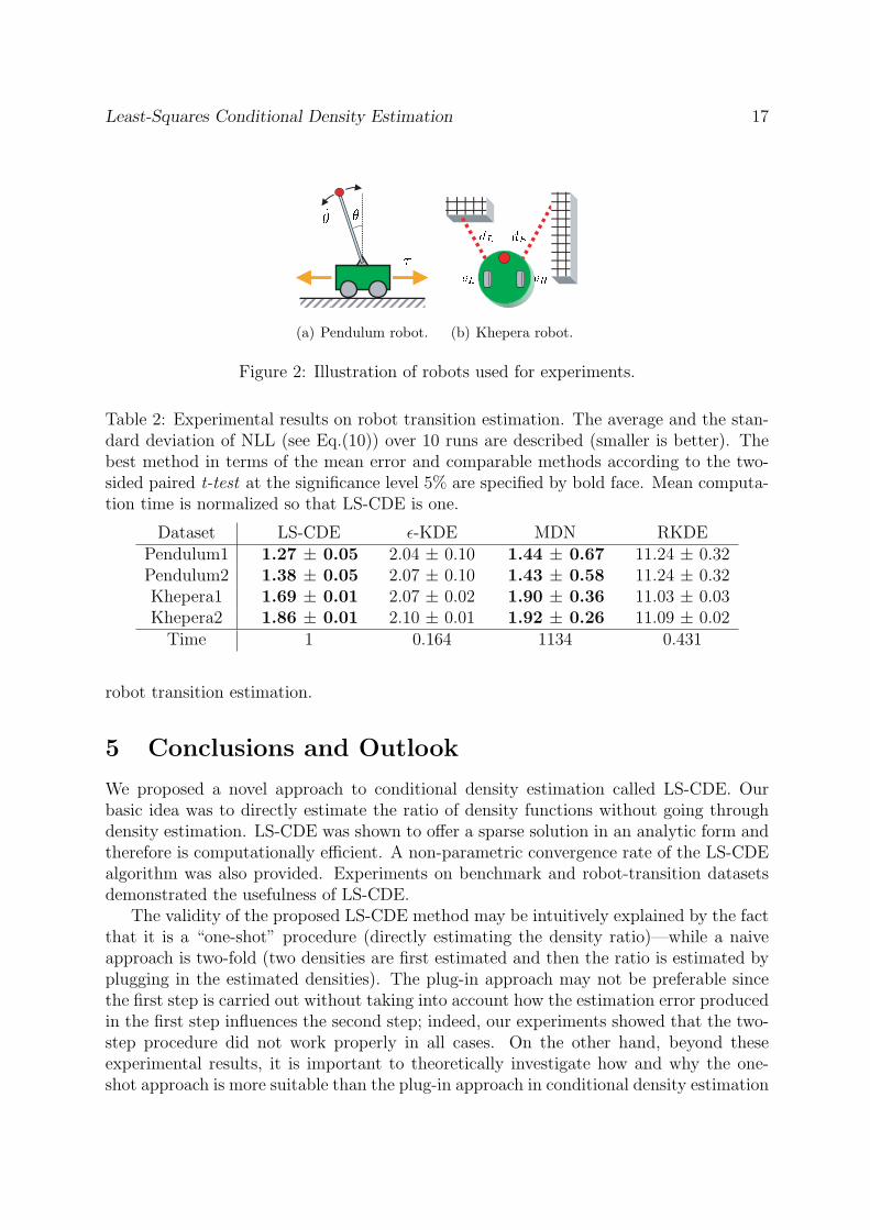
We further applied the proposed and existing methods to the problem of robot transitionestimation. We used the pendulum robot and the Khepera robot simulators illustratedin Figure 2.

The pendulum robot consists of wheels and a pendulum hinged to the body. Thestate of the pendulum robot consists of angle θ and angular velocity θ of the pendulum.The amount of torque τ applied to the wheels can be controlled, by which the robot canmove left or right and the state of the pendulum is changed to θ′ and θ′. The task is toestimate p(θ′, θ′|θ, θ, τ), the transition probability density from state (θ, θ) to state (θ′, θ′)by action τ .

The Khepera robot is equipped with two infra-red sensors and two wheels. Theinfra-red sensors dL and dR measure the distance to the left-front and right-front walls.The speed of left and right wheels vL and vR can be controlled separately, by whichthe robot can move forward/backward and rotate left/right. The task is to estimatep(d′L, d

′R|dL, dR, vL, vR), where d′L and d′R are the next state.

The state transition of the pendulum robot is highly stochastic due to slip, friction,or measurement errors with strong heteroscedasticity. Sensory inputs of the Kheperarobot suffer from occlusions and contain highly heteroscedastic noise, so the transitionprobability density may possess multi-modality and heteroscedasticity. Thus transitionestimation of dynamic robots is a challenging task. Note that transition estimation ishighly useful in model-based reinforcement learning [39].

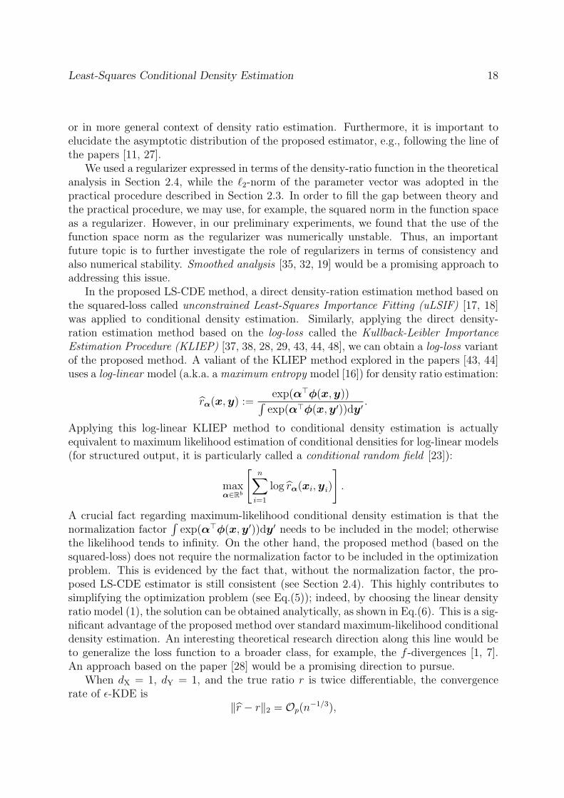
For both robots, 100 samples were used for conditional density estimation and addi-tional 900 samples were used for computing NLL (see Eq.(10)). The number of Gaussiancomponents was fixed to t = 3 in MDN, and all other tuning parameters were chosen byCV based on the Kullback-Leibler (KL) error (see Section 2.5). Experimental results aresummarized in Table 2, showing that LS-CDE is still useful in this challenging task of


(a) Pendulum robot. (b) Khepera robot.

Figure 2: Illustration of robots used for experiments.

Table 2: Experimental results on robot transition estimation. The average and the stan-dard deviation of NLL (see Eq.(10)) over 10 runs are described (smaller is better). Thebest method in terms of the mean error and comparable methods according to the two-sided paired t-test at the significance level 5% are specified by bold face. Mean computa-tion time is normalized so that LS-CDE is one.

Dataset LS-CDE ϵ-KDE MDN RKDEPendulum1 1.27 ± 0.05 2.04 ± 0.10 1.44 ± 0.67 11.24 ± 0.32Pendulum2 1.38 ± 0.05 2.07 ± 0.10 1.43 ± 0.58 11.24 ± 0.32Khepera1 1.69 ± 0.01 2.07 ± 0.02 1.90 ± 0.36 11.03 ± 0.03Khepera2 1.86 ± 0.01 2.10 ± 0.01 1.92 ± 0.26 11.09 ± 0.02Time 1 0.164 1134 0.431

robot transition estimation.

5 Conclusions and Outlook

We proposed a novel approach to conditional density estimation called LS-CDE. Ourbasic idea was to directly estimate the ratio of density functions without going throughdensity estimation. LS-CDE was shown to offer a sparse solution in an analytic form andtherefore is computationally efficient. A non-parametric convergence rate of the LS-CDEalgorithm was also provided. Experiments on benchmark and robot-transition datasetsdemonstrated the usefulness of LS-CDE.

The validity of the proposed LS-CDE method may be intuitively explained by the factthat it is a “one-shot” procedure (directly estimating the density ratio)—while a naiveapproach is two-fold (two densities are first estimated and then the ratio is estimated byplugging in the estimated densities). The plug-in approach may not be preferable sincethe first step is carried out without taking into account how the estimation error producedin the first step influences the second step; indeed, our experiments showed that the two-step procedure did not work properly in all cases. On the other hand, beyond theseexperimental results, it is important to theoretically investigate how and why the one-shot approach is more suitable than the plug-in approach in conditional density estimation


or in more general context of density ratio estimation. Furthermore, it is important toelucidate the asymptotic distribution of the proposed estimator, e.g., following the line ofthe papers [11, 27].

We used a regularizer expressed in terms of the density-ratio function in the theoreticalanalysis in Section 2.4, while the ℓ2-norm of the parameter vector was adopted in thepractical procedure described in Section 2.3. In order to fill the gap between theory andthe practical procedure, we may use, for example, the squared norm in the function spaceas a regularizer. However, in our preliminary experiments, we found that the use of thefunction space norm as the regularizer was numerically unstable. Thus, an importantfuture topic is to further investigate the role of regularizers in terms of consistency andalso numerical stability. Smoothed analysis [35, 32, 19] would be a promising approach toaddressing this issue.

In the proposed LS-CDE method, a direct density-ration estimation method based onthe squared-loss called unconstrained Least-Squares Importance Fitting (uLSIF) [17, 18]was applied to conditional density estimation. Similarly, applying the direct density-ration estimation method based on the log-loss called the Kullback-Leibler ImportanceEstimation Procedure (KLIEP) [37, 38, 28, 29, 43, 44, 48], we can obtain a log-loss variantof the proposed method. A valiant of the KLIEP method explored in the papers [43, 44]uses a log-linear model (a.k.a. amaximum entropy model [16]) for density ratio estimation:

rα(x,y) :=exp(α⊤ϕ(x,y))∫exp(α⊤ϕ(x,y′))dy′ .

Applying this log-linear KLIEP method to conditional density estimation is actuallyequivalent to maximum likelihood estimation of conditional densities for log-linear models(for structured output, it is particularly called a conditional random field [23]):

maxα∈Rb

[n∑

i=1

log rα(xi,yi)

].

A crucial fact regarding maximum-likelihood conditional density estimation is that thenormalization factor

∫exp(α⊤ϕ(x,y′))dy′ needs to be included in the model; otherwise

the likelihood tends to infinity. On the other hand, the proposed method (based on thesquared-loss) does not require the normalization factor to be included in the optimizationproblem. This is evidenced by the fact that, without the normalization factor, the pro-posed LS-CDE estimator is still consistent (see Section 2.4). This highly contributes tosimplifying the optimization problem (see Eq.(5)); indeed, by choosing the linear densityratio model (1), the solution can be obtained analytically, as shown in Eq.(6). This is a sig-nificant advantage of the proposed method over standard maximum-likelihood conditionaldensity estimation. An interesting theoretical research direction along this line would beto generalize the loss function to a broader class, for example, the f -divergences [1, 7].An approach based on the paper [28] would be a promising direction to pursue.

When dX = 1, dY = 1, and the true ratio r is twice differentiable, the convergencerate of ϵ-KDE is

∥r − r∥2 = Op(n−1/3),


given that the bandwidth ϵ is optimally chosen [15]. On the other hand, Theorem 1and the discussions before the theorem in the current paper imply that our method canachieve

Op(n− 1

(dX+dY)/p+2 log n) = Op(n− 1

2/p+2 log n),

where p ≥ 2. Therefore, if we choose a model such that p > 2 and the true ratio r iscontained, the convergence rate of our proposed method dominates that of ϵ-KDE. Thisis because ϵ-KDE just takes the average around the target point x and hence it does notcapture higher order smoothness of the target conditional density. On the other hand,our method can utilize the information of higher order smoothness by properly choosingthe degree of smoothness with cross-validation.

In the experiments, we used the common width for all Gaussian basis functions (9)in the proposed LS-CDE procedure. As shown in Section 2.4, the proposed methodis consistent even with the common Gaussian width. However, in practice, it may bemore flexible to use different Gaussian widths for different basis functions. Althoughour method in principle allows the use of different Gaussian widths, this in turn makescross-validation computationally harder. A possible measure for this issue would be toalso learn the Gaussian widths from the data together with coefficients. An expectation-maximization approach to density ratio estimation based on the log-loss for Gaussianmixture models has been explored [48], which allows us to learn the Gaussian covariancesin an efficient manner. Developing a squared-loss variant of this method could produce auseful variant of the proposed LS-CDE method.

As explained in Section 2.7, LS-CDE can take advantage of the semi-supervised learn-ing setup [5], although this was not explored in the current paper. Thus it is important toinvestigate how the performance of LS-CDE is improved under semi-supervised learningscenarios both in theoretically and experimentally.

Although we focused on conditional density estimation in this article, one may haveinterests in substantially simpler tasks such as error bar estimation and confidential in-terval estimation. Investigating whether the current line of research can be adapted tosolving such simpler problems with higher accuracy is an important future issue.

Even though the proposed approach was shown to work well in experiments, its per-formance (and also the performance of any other non-parametric approaches) is still poorin high-dimensional problems. Thus, a further challenge is to improve the accuracy inhigh-dimensional cases. Application of a dimensionality reduction idea in density ratioestimation [36] would be a promising direction to address this issue.

Another possible future work from the application point of view would be the use of theproposed method in reinforcement learning scenarios, since a good transition model can bedirectly used for solving Markov decision problems in continuous and multi-dimensionaldomains [24, 39]. Our future work will explore this issue in more detail.


Acknowledgments

We thank fruitful comments from anonymous reviewers. MS was supported by AOARD,SCAT, and the JST PRESTO program.

References

[1] S.M. Ali and S.D. Silvey, “A general class of coefficients of divergence of one distri-bution from another,” Journal of the Royal Statistical Society, Series B, vol.28, no.1,pp.131–142, 1966.

[2] A. Basu, I.R. Harris, N.L. Hjort, and M.C. Jones, “Robust and efficient estimationby minimising a density power divergence,” Biometrika, vol.85, no.3, pp.540–559,1998.

[3] S. Bickel, M. Bruckner, and T. Scheffer, “Discriminative learning for differing trainingand test distributions,” Proceedings of the 24th International Conference on MachineLearning, pp.81–88, 2007.

[4] C.M. Bishop, Pattern Recognition and Machine Learning, Springer, New York, NY,USA, 2006.

[5] O. Chapelle, B. Scholkopf, and A. Zien, eds., Semi-Supervised Learning, MIT Press,Cambridge, 2006.

[6] K.F. Cheng and C.K. Chu, “Semiparametric density estimation under a two-sampledensity ratio model,” Bernoulli, vol.10, no.4, pp.583–604, 2004.

[7] I. Csiszar, “Information-type measures of difference of probability distributionsand indirect observation,” Studia Scientiarum Mathematicarum Hungarica, vol.2,pp.229–318, 1967.

[8] A.P. Dempster, N.M. Laird, and D.B. Rubin, “Maximum likelihood from incompletedata via the EM algorithm,” Journal of the Royal Statistical Society, series B, vol.39,no.1, pp.1–38, 1977.

[9] D. Edmunds and H. Triebel, eds., Function Spaces, Entropy Numbers, DifferentialOperators, Cambridge Univ Press, 1996.

[10] J. Fan, Q. Yao, and H. Tong, “Estimation of conditional densities and sensitivitymeasures in nonlinear dynamical systems,” Biometrika, vol.83, no.1, pp.189–206,1996.

[11] S. Geman and C.R. Hwang, “Nonparametric maximum likelihood estimation by themethod of sieves,” The Annals of Statistics, vol.10, no.2, pp.401–414, 1982.


[12] W. Hardle, M. Muller, S. Sperlich, and A. Werwatz, Nonparametric and Semipara-metric Models, Springer, Berlin, 2004.

[13] T. Hastie, R. Tibshirani, and J. Friedman, The Elements of Statistical Learning:Data Mining, Inference, and Prediction, Springer, New York, 2001.

[14] J. Huang, A. Smola, A. Gretton, K.M. Borgwardt, and B. Scholkopf, “Correctingsample selection bias by unlabeled data,” in Advances in Neural Information Pro-cessing Systems 19, ed. B. Scholkopf, J. Platt, and T. Hoffman, pp.601–608, MITPress, Cambridge, MA, 2007.

[15] R.J. Hyndman, D.M. Bashtannyk, and G.K. Grunwald, “Estimating and visualiz-ing conditional densities,” Journal of Computational and Graphical Statistics, vol.5,no.4, pp.315–336, 1996.

[16] E.T. Jaynes, “Information theory and statistical mechanics,” Physical Review,vol.106, no.4, pp.620–630, 1957.

[17] T. Kanamori, S. Hido, and M. Sugiyama, “Efficient direct density ratio estimation fornon-stationarity adaptation and outlier detection,” Advances in Neural InformationProcessing Systems 21, ed. D. Koller, D. Schuurmans, Y. Bengio, and L. Botton,Cambridge, MA, pp.809–816, MIT Press, 2009.

[18] T. Kanamori, S. Hido, and M. Sugiyama, “A least-squares approach to direct im-portance estimation,” Journal of Machine Learning Research, vol.10, pp.1391–1445,Jul. 2009.

[19] T. Kanamori, T. Suzuki, and M. Sugiyama, “Condition number analysis of kernel-based density ratio estimation,” Tech. Rep. TR09-0006, Department of ComputerScience, Tokyo Institute of Technology, Feb. 2009.

[20] G.S. Kimeldorf and G. Wahba, “Some results on Tchebycheffian spline functions,”Journal of Mathematical Analysis and Applications, vol.33, no.1, pp.82–95, 1971.

[21] A.N. Kolmogorov and V.M. Tikhomirov, “ε-entropy and ε-capacity of sets in func-tion spaces,” American Mathematical Society Translations, vol.17, no.2, pp.277–364,1961.

[22] S. Kullback and R.A. Leibler, “On information and sufficiency,” Annals of Mathe-matical Statistics, vol.22, pp.79–86, 1951.

[23] J. Lafferty, A. McCallum, and F. Pereira, “Conditional random fields: Probabilisticmodels for segmenting and labeling sequence data,” Proceedings of the 18th Inter-national Conference on Machine Learning, pp.282–289, 2001.

[24] M.G. Lagoudakis and R. Parr, “Least-squares policy iteration,” Journal of MachineLearning Research, vol.4, pp.1107–1149, 2003.


[25] Y. Li, Y. Liu, and J. Zhu, “Quantile regression in reproducing kernel Hilbert spaces,”Journal of the American Statistical Association, vol.102, no.477, pp.255–268, 2007.

[26] A. Luntz and V. Brailovsky, “On estimation of characters obtained in statisticalprocedure of recognition,” Technicheskaya Kibernetica, vol.3, 1969. in Russian.

[27] W.K. Newey, “Convergence rates and asymptotic normality for series estimators,”Journal of Econometrics, vol.70, no.1, pp.147–168, 1997.

[28] X. Nguyen, M. Wainwright, and M. Jordan, “Estimating divergence functionals andthe likelihood ratio by penalized convex risk minimization,” in Advances in Neural In-formation Processing Systems 20, ed. J.C. Platt, D. Koller, Y. Singer, and S. Roweis,pp.1089–1096, MIT Press, Cambridge, MA, 2008.

[29] X. Nguyen, M.J. Wainwright, and M.I. Jordan, “Nonparametric estimation of thelikelihood ratio and divergence functionals,” Proceedings of IEEE International Sym-posium on Information Theory, Nice, France, pp.2016–2020, 2007.

[30] J. Qin, “Inferences for case-control and semiparametric two-sample density ratiomodels,” Biometrika, vol.85, no.3, pp.619–639, 1998.

[31] R Development Core Team, The R Manuals, 2008. http://www.r-project.org.

[32] A. Sankar, D.A. Spielman, and S.H. Teng, “Smoothed analysis of the condition num-bers and growth factors of matrices,” SIAM Journal on Matrix Analysis and Appli-cations, vol.28, no.2, pp.446–476, 2006.

[33] B. Scholkopf and A.J. Smola, Learning with Kernels, MIT Press, Cambridge, MA,2002.

[34] D.W. Scott, “Remarks on fitting and interpreting mixture models,” Computing Sci-ence and Statistics, vol.31, pp.104–109, 1999.

[35] D.A. Spielman and S.H. Teng, “Smoothed analysis of algorithms: Why the simplexalgorithm usually takes polynomial time,” Journal of the ACM, vol.51, no.3, pp.385–463, 2004.

[36] M. Sugiyama, M. Kawanabe, and P.L. Chui, “Dimensionality reduction for densityratio estimation in high-dimensional spaces,” Neural Networks, vol.23, no.1, pp.44–59, 2010.

[37] M. Sugiyama, S. Nakajima, H. Kashima, P. von Bunau, and M. Kawanabe, “Directimportance estimation with model selection and its application to covariate shiftadaptation,” Advances in Neural Information Processing Systems 20, ed. J.C. Platt,D. Koller, Y. Singer, and S. Roweis, Cambridge, MA, pp.1433–1440, MIT Press,2008.


[38] M. Sugiyama, T. Suzuki, S. Nakajima, H. Kashima, P. von Bunau, and M. Kawanabe,“Direct importance estimation for covariate shift adaptation,” Annals of the Instituteof Statistical Mathematics, vol.60, no.4, pp.699–746, 2008.

[39] R.S. Sutton and G.A. Barto, Reinforcement Learning: An Introduction, MIT Press,Cambridge, MA, 1998.

[40] I. Takeuchi, Q.V. Le, T.D. Sears, and A.J. Smola, “Nonparametric quantile estima-tion,” Journal of Machine Learning Research, vol.7, pp.1231–1264, 2006.

[41] I. Takeuchi, K. Nomura, and T. Kanamori, “Nonparametric conditional density es-timation using piecewise-linear solution path of kernel quantile regression,” NeuralComputation, vol.21, no.2, pp.533–559, 2009.

[42] V. Tresp, “Mixtures of gaussian processes,” Advances in Neural Information Pro-cessing Systems 13, ed. T.K. Leen, T.G. Dietterich, and V. Tresp, pp.654–660, MITPress, 2001.

[43] Y. Tsuboi, H. Kashima, S. Hido, S. Bickel, and M. Sugiyama, “Direct density ra-tio estimation for large-scale covariate shift adaptation,” Proceedings of the EighthSIAM International Conference on Data Mining (SDM2008), ed. M.J. Zaki, K. Wang,C. Apte, and H. Park, Atlanta, Georgia, USA, pp.443–454, Apr. 24–26 2008.

[44] Y. Tsuboi, H. Kashima, S. Hido, S. Bickel, and M. Sugiyama, “Direct density ratioestimation for large-scale covariate shift adaptation,” Journal of Information Pro-cessing, vol.17, pp.138–155, 2009.

[45] A.W. van der Vaart and J.A. Wellner, Weak Convergence and Empirical Processeswith Applications to Statistics, Springer, New York, NY, USA, 1996.

[46] S. Weisberg, Applied Linear Regression, John Wiley, New York, NY, USA, 1985.

[47] R.C.L. Wolff, Q. Yao, and P. Hall, “Methods for estimating a conditional distributionfunction,” Journal of the American Statistical Association, vol.94, no.445, pp.154–163, 1999.

[48] M. Yamada and M. Sugiyama, “Direct importance estimation with Gaussian mix-ture models,” IEICE Transactions on Information and Systems, vol.E92-D, no.10,pp.2159–2162, 2009.

[49] D.X. Zhou, “The covering number in learning theory,” Journal of Complexity archive,vol.18, no.3, pp.739–767, 2002.

Least-Squares Conditional Density · PDF fileLeast-Squares Conditional Density Estimation 3...

Documents

Transcript of Least-Squares Conditional Density · PDF fileLeast-Squares Conditional Density Estimation 3...