Pressure distribution under atwo-dimensional sandpile

二次元空間内の砂山底面での圧力分布に関する数値計算

S.Inagaki (稲垣紫緒) $*$

Dept. of $Mathematic\overline{a}\iota$ Sciences, Ibaraki University, Mito, Japan茨城大学大学院理工学研究科数理科学専攻

ABSTRACT: In the experiments about a pressure distribution undera sandpile, an interesting phenomenon was previously found. Just underthe apex of a pile, a vertical pressure minimum, called a dip, may be seen.Whether a dip appears or not depends on the way grains are poured.Dip is reproduced in our numerical experiment with a distinct elementmethod (DEM) that is a kind of molecular dynamics simulation. Wechoose tw.o different methods of supplying grains and compare the results(e.g., the distributions of the resulting contact force direction, Coulombangle distributions) as well as the pressures in order to recognize thedifference between the piles with two different histories. We made surethat the Coulomb angle distribution is thought to be connected with adip.

1 IntroductionConcerning granular materials, there is no clear boundary between

the states (gas, liquid, and solid). Energy is always dissipated by thecollisions of grains. By the energy dissipation, clusters are formed locally,and a homogeneous state is hardly kept dynamically. Energy supply is

*shio@mail.ne.jp

数理解析研究所講究録1184巻 2001年 140-151 140

perpetually needed to keep a steady state. Once the supply is halted,kinetic energy is completely lost, and a static state is obtained.

In a dynamical state, the interactions between grains and the mediaaround them, liquid or gas, are too complex to analyze directly. In thispaper, we focus on a static state, and reproduce a dip and make it clearhow the stresses propagate through granular media with DEM, a kind ofmolecular dynamics simulation.

2 Stress propagation inside a pileAmong various static states of granular matter, the simplest setting is a

pile constructed by just pouring grains on a floor. You can see a sandpileat a beach, or in a desert. Such a pile exhibits a certain characteristicangle called an angle of repose. It depends on a boundary condition,humidity, a particle shape, etc. The mechanism for the angle of reposestill remains unknown. In contrast, in the case of liquid drop on a floor,it takes a shape like a dome due to surface tension. On the other hand,the overall shape of a lot of water just extend flatly without making apile.

There are some previous research (e.g., $[3],[10],[17],[19]$ ) on reportingan interesting phenomenon called a “dip” under piles made of such gran-ular materials, as rape seeds, sands, frosted grass beads, lead shots, etc.For instance, Vanel et $al.[19]$ poured sands from a point source and raisedthe source gradually as a pile grew up. The pressure distribution alongthe bottom non-intuitively showed a local minimum just under the apexof a pile. Their experiment also showed the dependency of a dip on thehistory of how sands were poured. By constructing piles with a pointsource but at a fixed height, the dip became deeper than the one pouredfrom the rising point source. In contrast, when grains were supplied ho-mogeneously like a rain using a sieve, a dip never appeared despite thesimilarity in the overall shape of the piles created in both methods.

Many hypothesis (e.g., $[2],[5],[20]$ ) and models (e.g., $[12],[13],[15]$ ) havebeen proposed in attempts to explain and reproduce a dip. In this pa-per, we numerically compare the two types of grain sources in order to

141

investigate the history dependence.

3 Distinct Element MethodDEM is a method commonly used, for instance, in manufacturing en-

gineering. Since the paper by Cundall and Struck [4], it has also beenused from the scientific point of view in simulating granular dynamics.DEM is to trace the movements of each grain like the description of La-grange. The main idea of the method is to solve many-body problemsby considering two-body interactions at the moment of contact, based onNewton ’s equation of motion $(\vec{F}=m\vec{a})$ .

Although DEM has problems left in details of modeling contact forces,the method is very intuitive, and constitutive equations commonly usedin a continuous description are never needed. A continuous model wouldprovide a platform easily treated in a theoretical analysis. However,the effect of the grain size is lost by coarse-grained averaging. Suchmicro-mechanical effects are supposed to have an important role in themacroscopic granular behavior. DEM can take these effects into accountnaturally. Assumptions have to be made on modeling contact forces andtuning parameters, but many kinds of phenomena (e.g., plugging in a$\mathrm{f}\mathrm{l}\mathrm{o}\mathrm{w}[16],$ $\mathrm{d}\mathrm{i}\mathrm{l}\mathrm{a}\mathrm{t}\mathrm{a}\mathrm{n}\mathrm{C}\mathrm{y}[9]$, flows in a $\mathrm{c}\mathrm{h}\mathrm{u}\mathrm{t}[11]$ , convection and fluidization ina vibrated $\mathrm{b}\mathrm{e}\mathrm{d}[18])$ have been reproduced by DEM. We can use it as avery powerful tool to understand the mechanism of behavior of granularmaterials. There is constantly an effort to construct a model with simplecontact forces but applicable in wide situations.

As mentioned in Sect.2, in the case of the simplest setting, a pile on afloor, we carry out a numerical calculation with DEM. Two-dimensionaldiscs are piled up on a floor, and the pressure at the bottom is measured.Using DEM with polygonal grains and a smooth bottom, the experimen-tal results have been already reproduced.[13] In this article, we show adip also even with perfectly round particles (discs) and a rough bottom,decreasing the number of the parameters in the model.

142

3.1 Model

Contact forces are calculated at each contact point, and a resultingforce acting on each grain is the sum of the contact force vectors for thatgrain. This enables us to solve the equations of motion time by time.In our model, the following three kinds of contact forces are taken intoaccount, in addition to the gravitational force. [8]

1. elastic force, proportional to the relative displacement between grains

2. viscous force, proportional to the relative velocity between grains3. rolling friction, proportional to each contact area and the relative

rotational velocity

For the tangential components, contributions from translational as wellas rotational motions are included. The total contact force is the sum ofthe three. The tangential component is cut off at a threshold known asthe Coulomb friction as follows;

$F_{t}\leq\mu F_{n}$ (1)

where $F_{t}$ and $F_{n}$ denote tangential and normal components of the totalforce, and $\mu$ is the coefficient of Coulomb friction.

Introduction of the rolling friction follows the modification of DEM byIwashita et $al.[9]$ as a possible cause for propagation of rotational mo-ments. Granular materials are deformed by the translational movementand the rotation of grains. Before, it had been regarded that the slip wasthe main effect of the deformation, and the rotational movement hadnot been considered. But Oda et $al.[14]$ showed the importance of therotations in the development of dilatanc.$\mathrm{y}$ in their experiment. Moreover,Bardet et $al.[1]$ showed by their numerical investigation that the rota-tion of grains concentrated near the shear bands, and there was a highgradient of particle rotation along the shear band boundaries Therefore,rotational movement of grains is here regarded important.

In this simulation, it can be expected that the shear forces act moreeffectively to convey energy of the surface flow into a pile by introducingthe rotational friction. Both in the dynamics and statics of granular

143

materials, microscopic friction between grains in contact should in nodoubt have great effect. Since details are still unknown, however, thestatic friction is not introduced explicitly in our model.

3.2 Calculation

We follow the algorithm of A.Shimosaka [21] and H.Hayakawa [7]. Thegoverning equations are non-dimensionalized in order to decrease thenumber of parameters in the equations. The characteristic length andtime scales are $d$ and $\sqrt{d/g}$ , respectively, so that the maximum diameterof the grain as well as the gravitational acceleration are both taken to beunity. We adopt the Euler scheme with second order accuracy for timeupdating of positions, velocities, and angular velocities of grains with thetime step $\delta t=1.0\cross 10^{-4}$ in the dimensionless unit. Actual values of theconstants used in this calculation are taken from the note [7]. By thismethod, we solve the equations of motion of each grain with the sum ofthe contact forces and the gravitational force.

In this paper, two kinds of methods for supplying grains are carried

$\mathrm{E}^{\backslash }1$ : Configurations of the grains. (Upper: Method 1, with 420 grains.Lower: Method 2, with 529 grains). . 4

144

out in order to make a comparison with the experiment by Vanel $et$

al. [19]. For the “point source”, we deposit a pack of grains (6 grains, inthis calculation) at a time interval (2.5 time units) in between, from thecenter of the computational domain, a little above the top of a pile (1space unit higher). Then we gradually raise the source to keep the samedistance from the top all the time. In the following, we call it Method 1.Although we had better carry out a numerical experiment with a fixedheight source in order to get a clearer dip, we have to do with a raisingsource because of the instability caused by the excess energy of grains.

On the other hand, Method 2 uses a homogeneous rain source. Grainsare poured layer by layer with the same time interval with Method 1.The width of a layer is gradually decreased as the pile grows. The layersare also released from the adjusted height like in Method 1.

3.3 Results

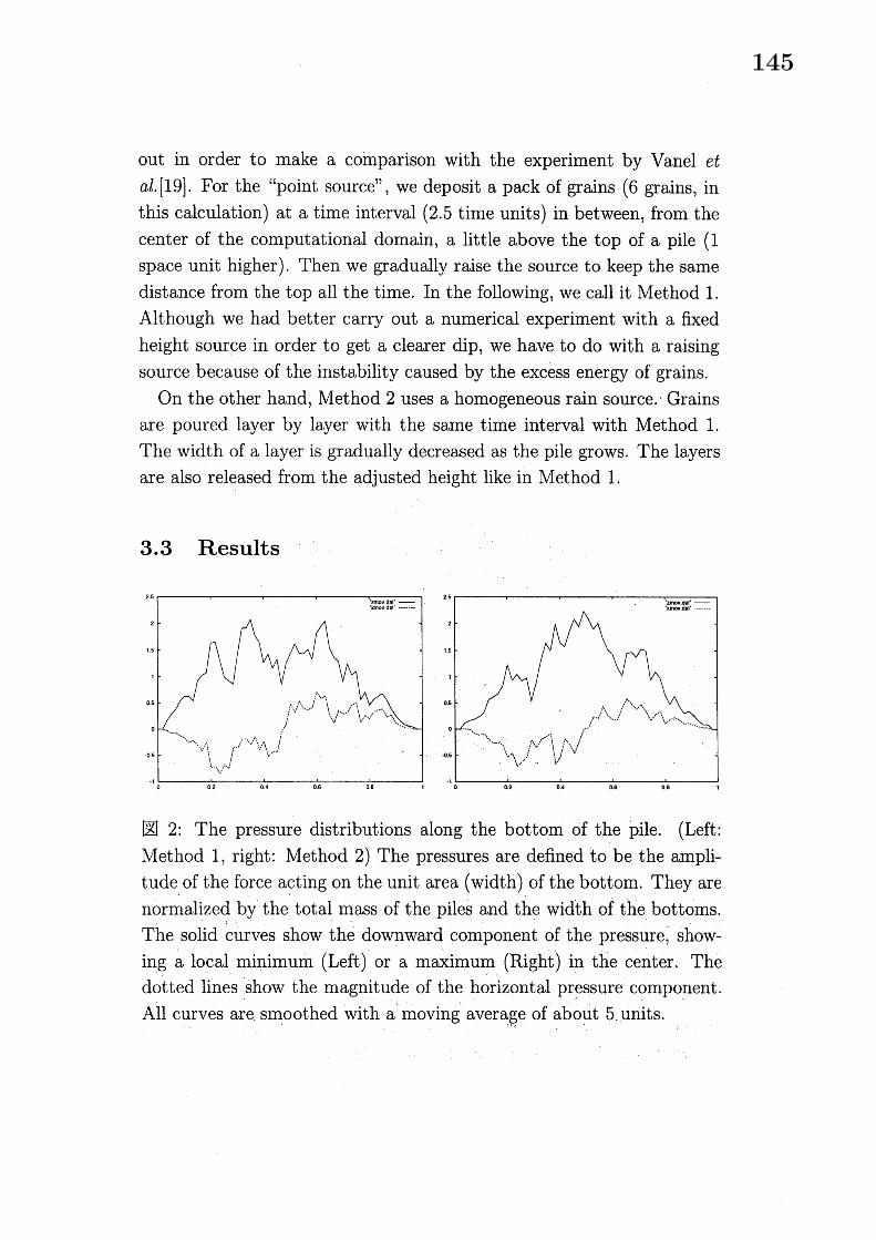
$\grave{\grave{y}}(2$ : The pressure distributions along the bottom of the pile. (Left:Method 1, right: Method 2) The pressures are defined to be the ampli-tude of the force acting on the unit area (width) of the bottom. They arenormalized by- the total mass of the piles arid the width $0\dot{\mathrm{f}}\mathrm{t}’ \mathrm{h}\mathrm{e}$ bottoms.The solid $\mathrm{c}\mathrm{u}\mathrm{r}\mathrm{V}\mathrm{e}\mathrm{S}$

.show the downward component of the pressure, show-

ing a local minimum (Left) or a maximum (Right) in the center. Thedotted lines show the magnitude of the horizontal pressure component.All curves are smoothed with a moving $\mathrm{a}\mathrm{v}\mathrm{e}\mathrm{r}\mathrm{a}\mathrm{g}_{r}\mathrm{e}$ of about 5 units.

145

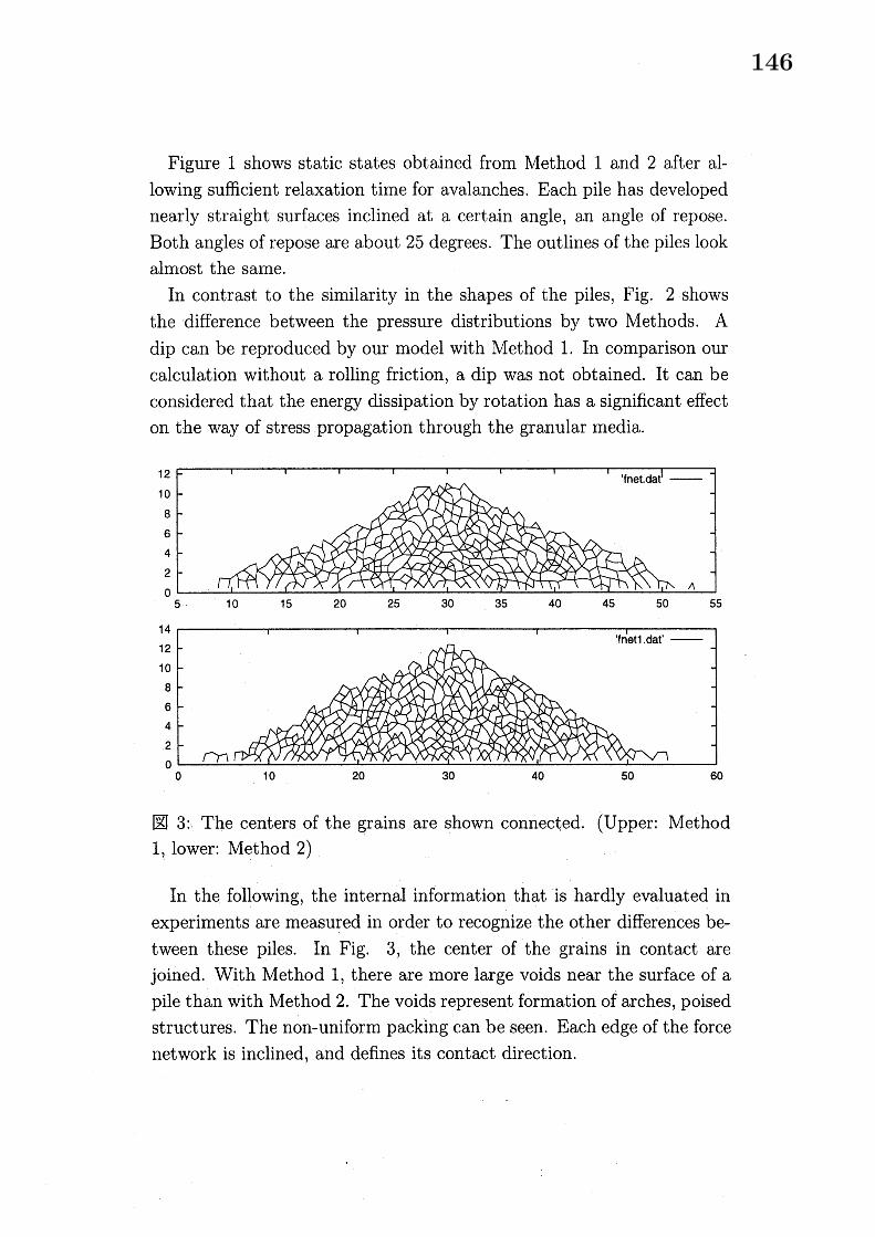
Figure 1 shows static states obtained from Method 1 and 2 after al-lowing sufficient relaxation time for avalanches. Each pile has developednearly straight surfaces inclined at a certain angle, an angle of repose.Both angles of repose are about 25 degrees. The outlines of the piles lookalmost the same.

In contrast to the similarity in the shapes of the piles, Fig. 2 showsthe difference between the pressure distributions by two Methods. Adip can be reproduced by our model with Method 1. In comparison ourcalculation without a rolling friction, a dip was not obtained. It can beconsidered that the energy dissipation by rotation has a significant effecton the way of stress propagation through the granular media.

$\backslash d3$ : The centers of the grains are shown connected. (Upper: Method1,. lower: Method 2)

In the following, the internal information that is hardly evaluated inexperiments are measured in order to recognize the other differences be-tween these piles. In Fig. 3, the center of the grains in contact arejoined. With Method 1, there are more large voids near the surface of apile than with Method 2. The voids represent formation of arches, poisedstructures. The non-uniform packing can be seen. Each edge of the forcenetwork is inclined, and defines its contact direction.

146

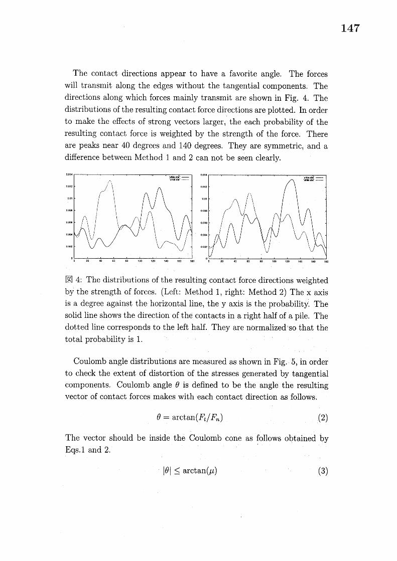
The contact directions appear to have a favorite angle. The forceswill transmit along the edges without the tangential components. Thedirections along which forces mainly transmit are shown in Fig. 4. Thedistributions of the resulting contact force directions are plotted. In orderto make the effects of strong vectors larger, the each probability of theresulting contact force is weighted by the strength of the force. Thereare peaks near 40 degrees and 140 degrees. They are symmetric, and adifference between Method 1 and 2 can not be seen clearly.

$\mathrm{E}^{\backslash }4$ : The distributions of the resulting contact force directions weightedby the strength of forces. (Left: Method 1, right: Method 2) The $\mathrm{x}$ axisis a degree against the horizontal line, the $\mathrm{y}$ axis is the probability. Thesolid line shows the direction of the contacts in a right half of a pile. Thedotted line corresponds to the left half. They are normalized so that thetotal probability is 1.

Coulomb angle distributions are measured as shown in Fig. 5, in orderto check the extent of distortion of the stresses generated by tangentialcomponents. Coulomb angle $\theta$ is defined to be the angle the resultingvector of contact forces makes with each contact direction as follows.

$\theta=\arctan(Ft/F_{n})$ (2)

The vector should be inside the Coulomb cone as follows obtained byEqs.1 and 2.

$|\theta|\leq\arctan(\mu)$ (3)

147

ot2 $012$$\mathrm{c}\mathrm{c}\mathrm{l}$ dr – $\mathrm{c}\mathrm{c}\mathrm{I}\mathrm{d}\cdot \mathrm{t}-$

$01$ 01

ooe ooe

ooe $0\alpha$

ou ou

$0M$ $0\infty$

$0_{1\infty}-$$\mathrm{r}$ $\alpha$ $\emptyset$ $0$ $n$ 10 . $\mathrm{r}$

,$\mathrm{r}$

$0_{1\Phi}.\alpha$ .. $.\alpha$ $.n$ $0$ a $\alpha$ $\alpha$ $\infty$ $\mathrm{t}\infty$

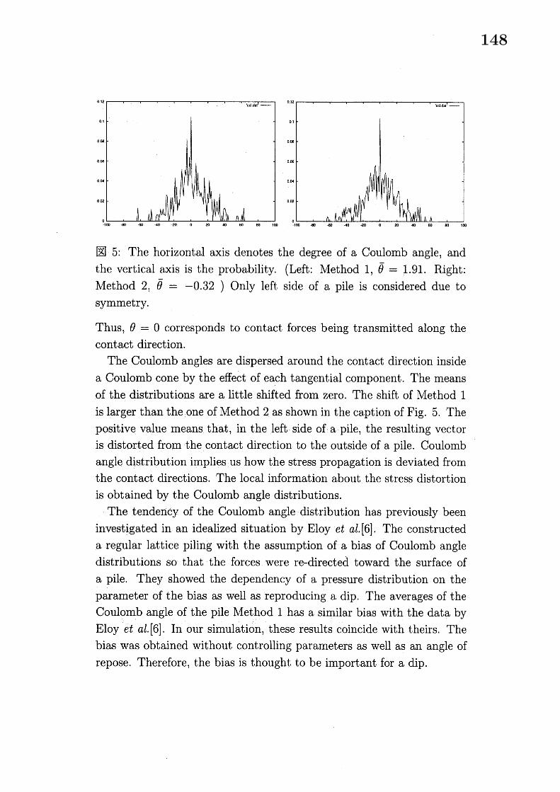
$5$ : The horizontal axis denotes the degree of a Coulomb angle, andthe vertical axis is the probability. (Left: Method 1, $\overline{\theta}=1.91$ . Right:Method 2, $\overline{\theta}=-0.32$ ) Only left side of a pile is considered due tosymmetry.

Thus, $\theta=0$ corresponds to contact forces being transmitted along thecontact direction.

The Coulomb angles are dispersed around the contact direction insidea Coulomb cone by the effect of each tangential component. The meansof the distributions are a little shifted from zero. The shift of Method 1is larger than the one of Method 2 as shown in the caption of Fig. 5. Thepositive value means that, in the left side of a pile, the resulting vectoris distorted from the contact direction to the outside of a pile. Coulombangle distribution implies us how the stress propagation is deviated fromthe contact directions. The local information about the stress distortionis obtained by the Coulomb angle distributions.

The tendency of the Coulomb angle distribution has previously beeninvestigated in an idealized situation by Eloy et $al.[6]$ . The constructeda regular lattice piling with the assumption of a bias of Coulomb angledistributions so that the forces were $\mathrm{r}\mathrm{e}$-directed toward the surface ofa pile. They showed the dependency of a pressure distribution on theparameter of the bias as well as reproducing a dip. The averages of theCoulomb angle of the pile Method 1 has a similar bias with the data byEloy et $al.[6]$ . In our simulation, these results coincide with theirs. Thebias was obtained without controlling parameters as well as an angle ofrepose. Therefore, the bias is thought to be important for a dip.

148

4 Open problemsAlthough a dip can be reproduced in our model, the modeling of con-

tact forces has mainly two problems left. The first is that although therolling friction is very intuitive, it has so far no physical evidence. If wecut off the rolling friction, and make the tangential viscous coefficientlarger, then it is possible that a dip will also appear. For the appear-ance of a dip, we need a large shear stress at each contact, and it canbe caused not only by the rolling friction. In order to simplification ofthe model, tangential components of contact forces should be united asmuch as possible.

As mentioned, another problem is that static friction is not includedyet explicitly in the model. But, in contrast with experiments, the be-havior of grains and the pressure distributions are well reproduced byour model, and the simpler model should be intended in order to analyzetheoretically.

On the $\mathrm{o}\mathrm{t}\dot{\mathrm{h}}\mathrm{e}\mathrm{r}$ hand, the average pressure distributions of many trialdoes not show so clear dip. Because the avalanches occurs left and rightby turns, and the mass center of a pile is fluctuated in horizontal direc-tion. We have to make sure with a larger pile so that the fluctuationwill be small enough against the width of a dip. In addition, there isa dependency of the pressure on the boundary condition. We have tocompare the boundar..y conditions as well as the ways to pour grains.

We intend to describe a stress propagation in a more general stylemacroscopically treating with the discreteness in space, for example byextending the boundary $\mathrm{c}\mathrm{o}\mathrm{n}\mathrm{d}\mathrm{i}\mathrm{t}\mathrm{i}_{0\mathrm{n}}$ to a vertical container, silo, based onthese results.

The author thank H.Hayakawa, E.Cl\’ement, and S.Watanabe for valu-able discussions.

149

参考文献

[1] Bardet, J.P., and Proube, J.: A numerical investigation of the struc-ture of persistent shear bands in granular media, G\’eotechnique, 41(1991) 599-613

[2] Bouchaud, J.P., Cates, M.E., and P.Claudin, P.: Stress distributionsin granular media and nonlinear wave equation, J.Phys.1 France 5(1995) 639-656

[3] Brockbank, R., Huntley, J.M., Ball, $\mathrm{R}.\mathrm{C}.$ : Contact force distributionbeneath a three-dimensional granular pile. J. Phys.2 France, 7 (1997)1521-1532

[4] Cundall, P.A., and Strack, $\mathrm{O}.\mathrm{D}$ .I.: A discrete numerical model forgranular assemblies. G\’eotechnique 29 (1979) 47-65

[5] Edwards, S.F., and Mounfield, $\mathrm{C}.\mathrm{C}.$ : A theoretical model for thestress distribution in $\mathrm{g}\mathrm{r}\mathrm{a}\mathrm{n}\mathrm{u}\dot{\mathrm{l}}\mathrm{a}\mathrm{r}$ matter.1. Basic equations, Physica$A,226$ (1996) 1

[6] Eloy, C., and Cl\’ement, E.: Stochastic aspects of the force networkin a regular granular piling. J. Phys. 1 France, 7 (1997) 1541-1558

[7] Hayakawa, H.: The distinct element method, in Japanese(unpublished but accessible at http://ace.phys.h.kyoto-

$\mathrm{u}.\mathrm{a}\mathrm{c}.\mathrm{j}\mathrm{p}/\mathrm{h}\mathrm{i}\mathrm{s}\mathrm{a}\mathrm{o}/\mathrm{j}\mathrm{p}\mathrm{a}\mathrm{p}\mathrm{e}\mathrm{r}\mathrm{S}/\mathrm{d}\mathrm{e}\mathrm{m}.\mathrm{p}\mathrm{S}.\mathrm{g}_{\mathrm{Z}})$

[8] Inagaki, S.: Pressure distribution of a two-dimensional sandpile,Proceeding of Traffic and Granular Flow ’99, (2000) (to be pub-lished)

[9] Iwashita, K., and Oda, M.: Rolling resistance at contacts in thesimulation of shear band development by DEM, J. $Eng$ . Mech, ASCE,No.124 (1998) 285-292

[10] Jyotaki,T., and Moriyama,R.: On the bottom pressure distributionof the bulk materials piled with the angle of repose, J. Soc. PowderTechnol. $Jpn60$ (1979) 184-191

150

[11] Kano, J., Shimosaka, A., and Hidaka, J.: Computer simulation ofthe flowing behavior of granular materials in a chute, J. Soc. PowderTech., $Jpn30$ (1993) 188

[12] Luding, S.: Stress distribution in static two-dimensional granularmodel media in the absence of friction, Phys. Rev. Lett. 55 (1997)4720

[13] Matuttis, H-G.: Simulation of the pressure distribution under a two-dimensional heap of polygonal particles, Granular Matter 1 (1998)83-91

[14] Oda, M., Konishi, J., and Nemat-Nasser, S.: Experimental micro-mechanical evaluation of strength of granular materials: Effect ofparticle rolling, Mechanics of Materials, 1 (1982) 263-283

[15] Oron, G., and $\mathrm{H}.\mathrm{J}$ .Herrmann, $\mathrm{H}.\mathrm{J}.$ : Exact calculation of force net-works in granular piles, Phys. Rev. $E,$ $58$ (1998) 2079

[16] Sakaguchi, H., and Igarashi T.$\cdot$ : Plugging of the Flow of GranularMaterials during the Discharge from a silo., Int. J. Mod. Phys. $B7$

(1993) 1949

[17] Smid, J., Novosad, J.: Pressure distribution under heaped bulksolids. I. Chem. E. Symposium Series 63 $\mathrm{D}3/\mathrm{V}/1$

[18] Taguchi, Y-h.: Phys. Rev. Lett. 69 (1992) 1367

[19] Vanel, L., Howell, D., Clark, D., Behringer, B.P., and Cl\’ement, E.:Effect of construction history on the stress distribution under a sandpile, Phys.Rev. Lett, 60 (1999) R5040-5043

[20] Wittmer, J.P., Cates, M.E., and Claudin, P.: Stress Propagationand Arching in Static Sandpiles, J. Phys.1 France, 7 (1997) 39-80

[21] The Society of Powder Technology, Japan Eds: Introduc-tion to granular simulation (Sangyo Tosho, Tokyo, 1998) inJapanese. (Funtai simulation Nyumon) Errata by A. Shimosaka :http: $//\mathrm{w}\mathrm{w}\mathrm{w}.\mathrm{i}\mathrm{i}\mathrm{j}\mathrm{n}\mathrm{e}\mathrm{t}.\mathrm{o}\mathrm{r}.\mathrm{j}\mathrm{p}/\mathrm{S}\mathrm{P}\mathrm{T}\mathrm{J}/\mathrm{S}_{0}\mathrm{C}\mathrm{P}_{0}\mathrm{w}\mathrm{T}\mathrm{e}\mathrm{C}/\mathrm{s}\mathrm{h}\mathrm{u}\mathrm{s}\mathrm{e}\mathrm{i}.\mathrm{h}\mathrm{t}\mathrm{m}1$

151