
Jeremy Nett
124
THE STUDY OF MS USING MRI, IMAGE PROCESSING, AND VISUALIZATION By Jeremy Michael Nett B.S.E.E., University of Louisville, 2000 A Thesis Submitted to the Faculty of the University of Louisville Speed Scientific School As Partial Fulfillment of the Requirements For the Professional Degree MASTER OF ENGINEERING Department of Electrical and Computer Engineering December, 2001
-
Upload
pedro-vieira -
Category
Documents
-
view
235 -
download
0
Transcript of Jeremy Nett
8/12/2019 Jeremy Nett
http://slidepdf.com/reader/full/jeremy-nett 1/124
THE STUDY OF MS USING MRI, IMAGE PROCESSING, AND VISUALIZATION
By
Jeremy Michael NettB.S.E.E., University of Louisville, 2000
A ThesisSubmitted to the Faculty of the
University of LouisvilleSpeed Scientific School
As Partial Fulfillment of the RequirementsFor the Professional Degree
MASTER OF ENGINEERING
Department of Electrical and Computer Engineering
December, 2001

8/12/2019 Jeremy Nett
http://slidepdf.com/reader/full/jeremy-nett 2/124
ii
THE STUDY OF MS USING MRI, IMAGE PROCESSING, AND VISUALIZATION
Submitted by:
Jeremy Michael Nett
A Thesis Approved on
By the Following Reading and Examination Committee:
Aly A. Farag, Thesis Director
Tom Cleaver
Kyung Kang
Robert Falk
Christina Kaufman
Stephen Hushek
8/12/2019 Jeremy Nett
http://slidepdf.com/reader/full/jeremy-nett 3/124
iii
ACKNOWLEDGMENTS
The author would like to thank all those that made his education at the University
of Louisville possible, including the many contributors to the scholarship funds of which
he was profoundly honored to be a recipient.
The author would also like to thank Dr. Aly Farag and the CVIP Lab for an
interesting thesis topic, and support during the completion of this work. Additionally, the
author would like to thank Dr. Robert Falk of Jewish Hospital for spending much of his
valuable time guiding this work, commenting on its quality, and for many suggestions on
how to make the tools developed more applicable in the setting of medical research and
clinical use. The author would also like to thank the additional members of his thesis
committee for their review and critique of his work, including Dr. Stephen Hushek of
Norton Healthcare, Dr. Christina Kaufman of the Institute for Cellular Therapeutics of
the School of Medicine at the University of Louisville, Dr. Thomas Cleaver of the
Electrical and Computer Engineering Department, and Dr. Kyung Kang of the Chemical
Engineering Department.
Last but not least, the author would like to sincerely thank his parents, Michael
and Kathy Nett, for putting up with him, and his grandmother, Agnita Nett, for a place to
stay. Without their support, this work would have not been possible.
8/12/2019 Jeremy Nett
http://slidepdf.com/reader/full/jeremy-nett 4/124
iv
ABSTRACT
Multiple sclerosis (MS), a well known disease of the nervous system in which the
myelin sheaths of axons are damaged, may be imaged using magnetic resonance imaging
(MRI) modalities. In this research, image analysis, volume registration, and scientific
visualization techniques are applied for quantitative and qualitative analysis of the
response of the disease to a proposed treatment regimen. Image analysis techniques are
applied, with the objective of automated and reliable quantitative evaluation of MS
lesions in the brain, through segmentation and classification of the brain and MS lesions.
To facilitate a time-series analysis of lesions, a volume registration technique is applied
to geometrically align MRI scans taken at different times over the course of treatment.
Additionally, scientific visualization techniques are utilized to facilitate three-
dimensional analysis of the disease pathology, and evaluation of changes in the structure
of lesions over a period of treatment. The result of these efforts is a preliminary system
for the study of MS using MRI.
8/12/2019 Jeremy Nett
http://slidepdf.com/reader/full/jeremy-nett 5/124
v
TABLE OF CONTENTS
PageAPPROVAL PAGE…………………………………………………………….. ii
ACKNOWLEDGMENTS……………………………………………………… iii
ABSTRACT……………………………………………………………………. iv
NOMENCLATURE……………………………………………………………. viii
LIST OF TABLES……………………………………………………………… xi
LIST OF FIGURES…………………………………………………………….. xii
I. INTRODUCTION……………………………………………………... 1
A. General Introduction……………………………………………. 1
B. Introduction to Multiple Sclerosis……………………………… 2
C. Introduction to Magnetic Resonance Imaging of MS………….. 2
D. Introduction to Computer-Assisted Evaluation of MS………… 5
E. Previous Work in MS Studies Using MRI and ImageProcessing Approaches…………………………………….. 7
F. Introduction to Lab Facilities and Data Acquisition……………. 9
G. Outline of the Components of the Researched Solution……….. 11
H. Summary……………………………………………………….. 12
II. VOLUME REGISTRATION…………………………………………. 13
A. Introduction to Volume Registration…………………………... 13
B. Imaging Model…………………………………………………. 19
C. Transformations………………………………………………... 26

8/12/2019 Jeremy Nett
http://slidepdf.com/reader/full/jeremy-nett 6/124
vi
D. Volume Interpolation …………………………………………... 30
E. Overview of Registration Approaches…………………………. 31
F. Registration Metric/Criteria……………………………………. 32
G. Computation of the Mutual Information Metric……………….. 37
H. Search Algorithm………………………………………………. 43
I. Implementation………………………………………………….. 44
J. Results: MS Studies…………………………………………….. 44
K. Summary……………………………………………………….. 50
III. BRAIN SEGMENTATION FROM THE HEAD……………………. 51
A. Introduction and Necessity…………………………………….. 51
B. Brain Segmentation Utilizing Registration…………………….. 52
C. Results: Manual a priori Segmentation………………………... 55
D. Results: Semi-Automatic a priori Segmentation………………. 59
E. Summary……………………………………………………….. 62
IV. TISSUE SEGMENTATION…………………………………………. 63
A. Introduction and Necessity……………………………………... 63
B. Feature Selection……………………………………………….. 64
C. Thresholding……………………………………………………. 67
D. Segmentation by Image Enhancement…………………………. 69
E. Segmentation by Unsupervised Clustering…………………….. 73
F. Bayesian Classification………………………………………… 77
G. Bayesian Classification: Gaussian Conditionals, Equal a priori Probabilities………………………………………………... 80
8/12/2019 Jeremy Nett
http://slidepdf.com/reader/full/jeremy-nett 7/124
vii
H. Bayesian Classification: Nonparametric Conditionals, a priori Probabilities Modeled by Markov Random Fields………… 82
I. Quantification…………………………………………………… 89
J. Accuracy………………………………………………………… 90
K. Summary……………………………………………………….. 91
V. VISUALIZATION……………………………………………………. 92
A. Introduction…………………………………………………….. 92
B. Visualization for the Study of Volume Registration…………… 92
C. Visualization for the Study of Volume Segmentation…………. 96
D. Web-Based Presentation of Results…………………………….. 98
E. Summary……………………………………………………….. 99
VI. CONCLUSIONS AND RECOMMENDATIONS…………………… 101
REFERENCES……….…………………………………………………………. 104
VITA……………………………………………………………………………. 109

8/12/2019 Jeremy Nett
http://slidepdf.com/reader/full/jeremy-nett 8/124
viii
NOMENCLATURE
l = a volume coordinate vector in the image coordinate system
w = a volume coordinate vector in the world coordinate system
c =coordinate vector locating the center of a volumeorthe number of states of nature
c(i) = a diffusion function
C = transformation matrix for alignment of the center of a volume tothe origin in the world coordinate system
V = transformation matrix for scaling a volume to account forspatial sampling rates
Γ = transformation matrix for accounting of a gantry angle
A i,w = transformation matrix for conversion of image to worldcoordinates
R = reference volume for registration
F =floating volume for registrationora random field
T = transformation matrix for translation
R x, R y, R z = axis-angle rotation matrices
R = transformation matrix for rotation
TFR = transformation matrix from image coordinates in the floatingvolume to the reference volume
lower_left_N1,lower_left_N2,lower_left_N3
= coordinates for alignment of a bounding cube for trilinearvolume interpolation

8/12/2019 Jeremy Nett
http://slidepdf.com/reader/full/jeremy-nett 9/124
ix
V(sample i) = interpolated sample from a volume for a sample coordinate ofsample i
delta x, delta y, delta z = translational differences between a coordinate to interpolate at,and a point that forms an origin for trilinear interpolation
weight i = a weight and index i for trilinear interpolation
sample i = a sample at index i in a bounding cube for trilinear interpolation
p(x), q(x) = a probability distribution function
D(p||q) = relative entropy
I(X, Y) = mutual information of the random variables X and Y
H(X) = entropy of the random variable X
Tα = a registration transformation with a parameter set α
h(·) = a histogram
µ =coordinates of a cluster center locationora parameter of a Gaussian distribution
x = a feature vector
d = the dimension of the feature vector x
ω = a state of nature, or class
P(ω i|x) = the a posteriori probability of class ω i given a featuremeasurement x
p(x| ω i) = the class conditional probability of observing a featuremeasurement x, given a class ω i

8/12/2019 Jeremy Nett
http://slidepdf.com/reader/full/jeremy-nett 10/124
x
P(ω i) = the a priori probability of observing the class ω i
Σ = a d x d covariance matrix
σ = standard deviation
µ’, σ’ = estimated mean and standard deviation parameters
δ(·) = a Parzen window function
n = number of training samples
N = a neighborhood structure
S = set of a random field
r = order of a neighborhood structure
Z = a partition function in a Gibbs distribution
U(f) = an energy function in a Gibbs distribution
f k,l = an observation at a lattice point in a random field
α, β1, β2 = parameters of the energy function U(f)
T = temperature parameter of a Gibbs distribution

8/12/2019 Jeremy Nett
http://slidepdf.com/reader/full/jeremy-nett 11/124
xi
LIST OF TABLES
I. Samples and sample weightings for trilinear interpolation………………... 31
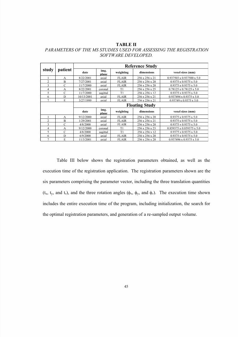
II. Parameters of the MS studies used for assessing the registration softwaredeveloped………………………………………………………………….. 45
III. Execution time and registration parameters for MS studies used…………. 46
IV. Quantification of MS disease burden from the sample results given infigure 25…………………………………………………………………… 90
8/12/2019 Jeremy Nett
http://slidepdf.com/reader/full/jeremy-nett 12/124
xii
LIST OF FIGURES
1. Sample slices from FLAIR MRI studies of patients with MS.Hyperintense regions in the brain are indicative of plaques caused by MS.. 4
2. The front-end to the patient database of Jewish Hospital…………………. 9
3. The SGI Onyx2 visual supercomputer used as a computing platform in thisresearch…………………………………………………………………….. 10
4. Illustration of the registration problem in two dimensions. The squares inthe left and right figures represent the respective scanning area. Comparedwith one another, the anatomy is located at a different position betweenthe two volumes, and has been rotated…………………………..……….... 14
5. Scout scans for the same patient, at different time points. Note that thelines that indicate the slice planes do not correspond in the two differentstudies……………………………………………………………….……… 15
6. Sample slice comparison between two scans of the same patient, taken atdifferent points in time. Each column contains sample slices from onestudy. The rows contain the same slice number from each study. Asapparent, the anatomy is not geometrically aligned between the twoscanning volumes…………………………………………………….…….. 16
7. Examples of sagittal scans (a), coronal scans(b), and axial scans (c)….…... 19
8. Formation a volume from an ordered set of images……………………….. 20
9. Illustration of eight samples in an isotropic volume. Each sample islocated at lattice points, with integer coordinates, and equal distances
between lattice locations which have a difference of 1.0 between acoordinate………………………………………………………………….. 22
10. Illustration of the parallel computation of the joint histogram necessary forcomputation of the mutual information metric…………………………….. 41
8/12/2019 Jeremy Nett
http://slidepdf.com/reader/full/jeremy-nett 13/124
xiii
11. Sample registration results from each of the seven MS data sets. The firstcolumn(a, d, g, j, m, p, and s) is a sample slice from the floating volumeused. The second column (b, e, h, k, n, q, and t) is the corresponding slicefrom the re-sampled reference volume. The third column (c, f, i, l, o, r,and u) is the checkerboard composite image of the two correspondingslices from the floating and re-sampled reference volumes. The floatingvolume and reference volumes used in each trial were from the same
patient……………………………………………………………………… 49
12. Samples of the (non-expert) manual segmentation of a patient’s brain fromthe remaining tissue of the head. The slices obtained from the MRI study((a), (b), and (c)) are manually segmented to obtain slices containing the
brain ((d), (e) and (f), respectively). The manually segmented images arethen made into binary masks ((g), (h), and (i), respectively)……………… 56
13. Registration of two MRI studies of the same patient, taken at differenttimes. The first study ((a), (b), and (c)) was manually segmented toextract the brain from the head. The second study ((d), (e), and (f)) wasregistered to the first (the re-sampled slices are shown)…………………… 57
14. Segmentation of the second study by a binary mask calculated from theregistration parameters, and the binary mask used to segment the a prioristudy. The raw input slices are shown ((a), (b), and (c)). The binary maskwas obtained by use of the registration parameters and the a priori mask((d), (e) and (f), respectively). By application of the mask, the segmentedvolume is obtained ((g), (h), and (i), respectively)……………………….. 58
15. Sample brain segmentation results of the a priori scan using a semi-automatic technique improved upon in the CVIP Lab. The input slices((a), (b), and (c)) are semi-automatically segmented to form a binary maskof the brain ((d), (e), and (f), respectively). The mask is then applied toform the segmented volume ((g), (h), and (i), respectively)………………. 60
16. Brain segmentation of the second study. The second study ((a), (b), and(c)) was registered to the a priori scan. The brain mask for the secondstudy ((d), (e), and (f), respectively) is then obtained using the a priori
brain mask, and the registration parameters. The binary brain mask is thenapplied to generate the segmented volume ((g), (h), and (i), respectively)... 61
17. A sample slice from an MRI study of an MS patient, with FLAIR (a andd), T1 (b and e), and T2 (c and f) weightings. The appearance of lesions isnot consistent between different weightings. MS lesions are easilyidentified in the FLAIR images as hyperintense regions in the brain……… 66
8/12/2019 Jeremy Nett
http://slidepdf.com/reader/full/jeremy-nett 14/124
xiv
18. Segmentation by thresholding. The input slice (a) is classified into threeclasses, based on selection of class on the interval in which an intensityfalls. Corresponding labeled image slice is shown in (b), with the darkgray indicating CSF, the light gray indicating normal brain material, andthe red indicating MS lesions……………………………………………… 68
19. The histogram of the input slice shown in figure 18 (a). Intervalscontaining a tissue class can be visually identified by a human. Peaking ofthe histogram at low intensities represents CSF, and at high intensities, MSlesions. Peaking of the histogram in the intermediate intensities indicatesnormal brain tissue…………………………………………………………. 68
20. Non-linear anisotropic diffusion filtering of MRI slices for segmentation.Input slices (a and c) are FLAIR weighted imagery. The correspondingoutput slices (b and d, respectively) show much enhanced images, but withthe loss of some MS lesions………………………………………………... 72
21. Illustration of types of errors encountered with segmentation via imageenhancement………………………………………………………………... 73
22. Results of k-means clustering, using 5 clusters. The input slice is shownin (a). The resulting clustered output image is shown in (b). By manualre-labeling of clusters such that clusters of similar tissue belong to thesame cluster, the output slice in (c) is obtained…………………………... 76
23. Sample result of tissue classification in the brain using a simple Bayesianclassifier, with equal a priori probabilities, and Gaussian class conditional
probabilities………………………………………………………………… 82
24. Neighborhood systems for an image modeled as a Markov random field…. 86
25. Sample classification results obtained using a Bayesian classifier, withclass conditional probabilities modeled nonparametrically, and class a
priori probabilities obtained from a Markov random field model of theimage. Input slices are shown in (a) and (c), and the classified images areshown in (b) and (d). In (b) and (d), normal brain material is indicated bythe color yellow, CSF by gray, and lesions as red…………………………. 89
26. Generation of the checkerboard image, by formation of a composite imageof square pixel regions from the re-sampled reference and floatingvolumes……………………………………………………………………. 93

8/12/2019 Jeremy Nett
http://slidepdf.com/reader/full/jeremy-nett 15/124
xv
27. Sample slices from different registration studies, showing the a slice fromthe floating volume ((a), (d), and (g)), corresponding slices from the re-sampled, registered reference volume ((b), (e),and (h), respectively), andthe checkerboard slices ((c), (f), and (i), respectively)…………………….. 94
28. Volume rendering and arbitrary volume re-slicing for comparison of twovolumes that are registered via maximization of mutual information……... 95
29. Frame interpolation ………………………………………………………... 96
30. A sample of a web page developed for presentation of the results of thisstudy on the Internet………………………………………………………... 99

8/12/2019 Jeremy Nett
http://slidepdf.com/reader/full/jeremy-nett 16/124
1
I. INTRODUCTION
A. General Introduction
The purpose of the research documented in this thesis is to provide for
quantitative, computer vision based evaluation of the disease burden of a patient suffering
from multiple sclerosis (MS), a debilitating disease of the human nervous system. This
computer vision system shall allow for highly-automated quantification of the disease
burden of a patient, based upon measurement of brain and lesion volumes of a patient.
Additionally, it is desirable to explore facilitation of qualitative evaluation of the disease,
and to allow such quantitative and qualitative approaches over the course of an extended
period of study, with imaging studies taken periodically.
The imaging studies that will be evaluated are magnetic resonance imaging (MRI)
studies of the human brain. These studies shall be administered at a local hospital, and
patient data transferred to local (laboratory-based) computing facilities for analysis.
Analysis shall consist of alignment of studies to a reference study, segmentation of the
head, brain, and lesions, and quantitative computation of brain and lesion volumes.
Additionally, scientific visualization techniques shall be applied to allow for comparison
of studies taken at different time points in the course of the study.
It should be noted that in the context of the medical study that this research
addresses, patients are known to have MS, and will more likely than not be in advanced
stages of the disease.

8/12/2019 Jeremy Nett
http://slidepdf.com/reader/full/jeremy-nett 17/124
2
B. Introduction to Multiple Sclerosis
Multiple sclerosis is a disease of the human central nervous system, affecting
approximately 250,000 to 350,000 people in the United States alone [1]. MS results in a
variety of clinically-observable deficiencies, such as speech difficulties, pain, impairment
of senses, loss of muscle control, and cognitive abnormalities [2].
In the brain, MS results in the inflammation and destruction of myelin, a fatty
covering insulating nerve cells [2]. This damage results in decreased ability of the
nervous system to control the body, leading to the clinically-observable symptoms of the
disease.
The causes of MS are not clearly accepted in the medical community.
Geographic, genetic, and environmental factors all seem to be present [1]. Many
researchers have proposed that MS is an autoimmune disease [1].
Though there are promising research developments, at this time, no cure is known
for this disease. Several treatment options are available, and allow for management of
the disease. Despite this, most patients progress in disability over the course of their life
[1]. Though not usually a fatal disease in and of itself, the resulting disabilities may
contribute to accidental mishaps [1].
C. Introduction to Magnetic Resonance Imaging of MS
Magnetic resonance (MR) imaging (MRI) is a medical imaging technology that
allows for non-invasive imaging of patient anatomy through the measurement of emitted
8/12/2019 Jeremy Nett
http://slidepdf.com/reader/full/jeremy-nett 18/124
3
nuclear magnetic resonance (NMR) signals. An MRI system is constructed of at least
three basic subsystems: a main magnet to produce a strong, homogenous, static field,
denoted as the B 0 field; a subsystem for generation of a gradient magnetic field, for signal
localization; and a radio-frequency (RF) subsystem, for generation and transmission of a
rotating magnetic field, denoted as the B 1 field, and measurement of NMR signals [3].
An MRI system evokes NMR signals from tissue to be imaged. By controlling
the acquisition parameters of the scan, different image weightings may be obtained,
allowing for different and/or improved image contrast between different types of tissue.
Image contrast in MRI studies is fundamentally based on the measurement of spin-lattice
relaxation (T1) time , spin-spin relaxation (T2) time , and nuclear spin density (PD).
Different types of images include T1-, T2-, PD-weighted images, and fluid
attenuated inversion recovery (FLAIR) images. A study is said to be a T1-weighted
study when the dominant tissue characteristic generating image contrast is the T1 time of
a tissue [3]. A study is said to be T2-weighted when the dominant tissue characteristic
generating image contrast is the T2 time of a tissue [3]. Finally, a study is said to be PD-
weighted when the dominant tissue characteristic generating image contrast is the nuclear
spin density of a tissue [3].
Inversion-recovery sequences are used to utilize T1 contrast, while allowing for
differentiation of tissues with approximately equal T2 times or nuclear spin densities [3].
FLAIR studies are implemented with inversion-recovery sequences designed to suppress
the intensity of cerebro-spinal fluid (CSF).
8/12/2019 Jeremy Nett
http://slidepdf.com/reader/full/jeremy-nett 19/124
4
When patients with MS are imaging using MRI modalities, lesions (also referred
to as plaques or deficits) can be contrasted against surrounding, normal brain tissue, by
choice of appropriate scan parameters, and depending on the state of the lesion [4].
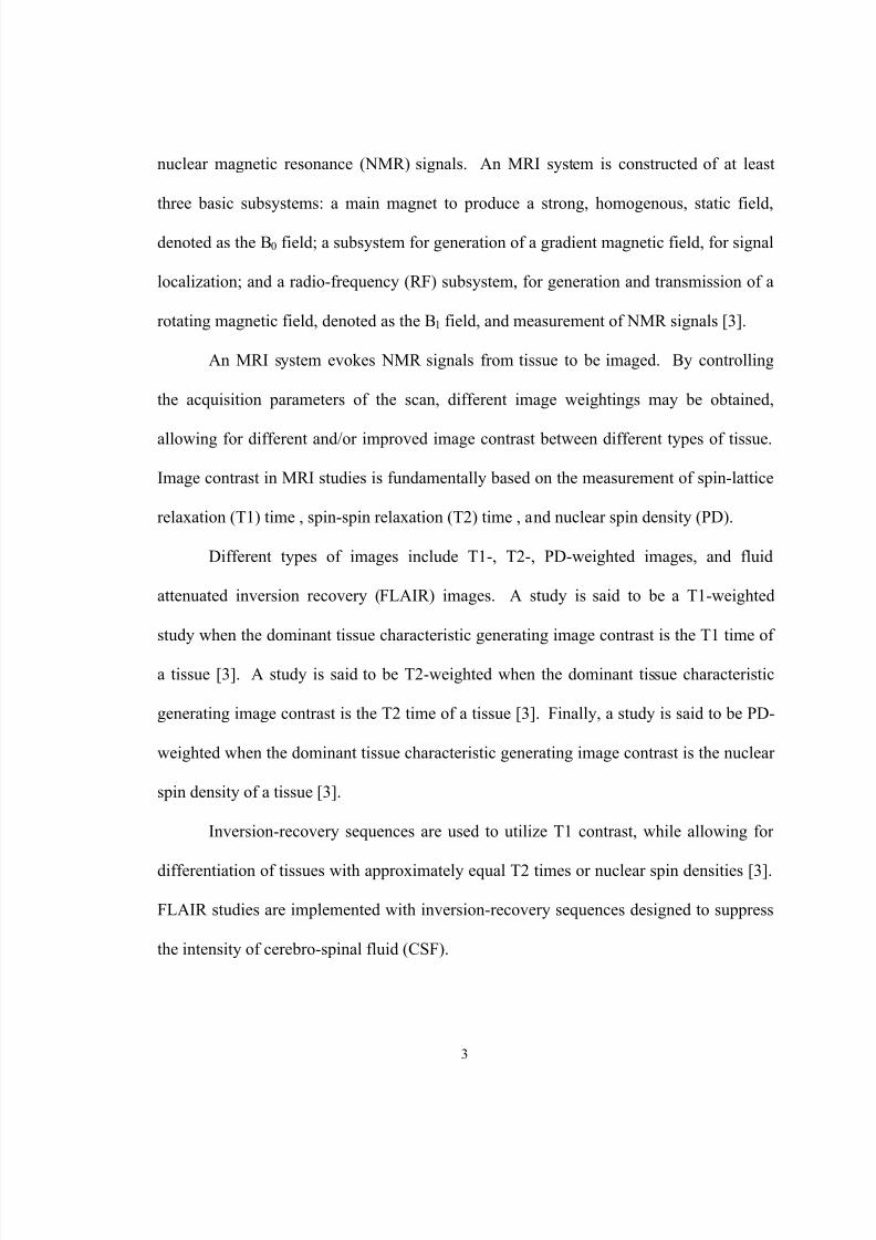
Figure 1 below shows several slices of different FLAIR MR images of patients
with MS. MS lesions appear as hyper intense regions in the patient's brain.
(a) (b)
(c) (d) FIGURE 1 : Sample slices from FLAIR MRI studies of patients with MS. Hyperintense
regions in the brain are indicative of plaques caused by MS.
The use of MR imagery in the evaluation of MS involves the identification of
abnormal brain tissue (MS lesions), and normal, non-diseased brain tissue (gray and
8/12/2019 Jeremy Nett
http://slidepdf.com/reader/full/jeremy-nett 20/124
8/12/2019 Jeremy Nett
http://slidepdf.com/reader/full/jeremy-nett 21/124
6
(CSF)) from the remaining tissues in the head (skull, skin, eyes, etc.). The second task is
to then segment the remaining imagery into CSF, normal brain material (gray and white
matter), and diseased brain tissue (here, MS lesions). Segmentation of the brain from the
remaining tissues image in the head allows for analysis of the brain only, and simplifies
this subsequent analysis. Segmentation of the remaining tissue into CSF, normal brain
tissue, and diseased tissue then allows for quantification of disease load.
There are several difficulties encountered with segmentation in the above context,
including noise, motion artifacts, limited spatial resolution, partial volume artifacts,
chemical shift artifacts, magnetic field inhomogeneity, and limited tissue contrast [3].
When a scan is taken of a patient, and later scans are taken, two factors must be
considered. First, scan parameters are likely to differ between scans, including voxel
dimensions, and perhaps scan weightings. Secondly, and most importantly, the patient
will not be positioned in the same location in the scanning volume. Thus, anatomy in two
different studies, taken with exactly the same scan parameters, will not be geometrically
aligned in the scanning volume, disallowing the possibility of comparing earlier and later
scans on a slice-by-slice basis. To allow for a comparison of multiple scans, a geometric
alignment of the anatomy imaged must be found; this function is known as volume
registration.
Difficulties encountered in volume registration include the same difficulties
encountered for segmentation.
8/12/2019 Jeremy Nett
http://slidepdf.com/reader/full/jeremy-nett 22/124
7
E. Previous Work in MS Studies Using MRI and Image Processing Approaches
Multiple sclerosis is a common enough disease, and with enough intrigue to
investigation of cures and treatments, that it has received a great deal of attention by a
number of research centers. Likewise, the disease and MR imaging of its victims has
received a fair amount of attention from several individuals and groups interested in the
application of computer vision techniques for analysis of such MR studies.
Several studies at notable institutions have incorporated computer analysis of
MRI studies of patients with MS. An extensive study and application of computer-aided
analysis was conducted at the Surgical Planning Laboratory at Brigham and Women’s
Hospital, of Boston, Massachusetts, U.S.A. [5, 6]. The system developed for the study
and quantification of MS utilizes an adaptive, statistical segmentation algorithm, known
as the expectation-maximization (EM) algorithm, for semi-automatic segmentation of
brain tissue. Three millimeter, continuous slices, weighted as PD and T2 scans are
acquired. Data is filtered, for noise smoothing. The brain is classified into four classes:
white matter, gray matter, CSF, and white matter lesions. Disease burden is evaluated by
computation of the volume of individual lesions and total lesion volume.
In [8], a brain tissue model is developed for segmentation of MRI studies of
patients with MS. The developed model is three-dimensional, voxel based, and provides
prior probabilities of white matter, gray matter, and CSF. In addition to providing prior
probabilities, the model-based approach is used to restrict the search for MS lesions to the
white matter of a patient’s brain. Also, as a part of [8], statistical and decision tree
classifiers are compared.

8/12/2019 Jeremy Nett
http://slidepdf.com/reader/full/jeremy-nett 23/124
8
The research documented in [9] segments brain tissue using a stochastic
relaxation method, originally developed for applications in image enhancement [10]. The
implemented algorithm, incorporating the use of the iterated conditional modes (ICM)
algorithm [10], claims to identify MS lesions in the white matter of a patient, and also
claims to perform a partial volume analysis of the resulting segmentation.
In [11], lesion segmentation is implemented by application of fuzzy objects and
fuzzy connected sets ideas [12], and the approach is semi-automatic. An operator selects
sample points for gray and white matter, and CSF, which then are detected in their
entirety by detection as a so-called fuzzy connected set. The voids in the union of these
tissue classes are potential lesions, which are presented to an operator for acceptance or
rejection as MS lesions.
In [13], an algorithm that is claimed to be fully automatic for segmentation of MS
lesions from MRI studies is presented. The general idea is for a model-aided, intensity-
based brain segmentation to proceed, as classification of gray and white matter, and
CSF. Features not well explained by the model are considered outliers, and are labeled as
MS lesions.
This previous work comprises a rich set of ideas from which to build upon, to
create an engineered system for quantitative and qualitative evaluation of MS using MRI,
in the local research community. There is opportunity for improvement and further
innovation, however, through classification of gray matter lesions, further automation,
and a more comprehensive approach to the study of MS.
8/12/2019 Jeremy Nett
http://slidepdf.com/reader/full/jeremy-nett 24/124
9
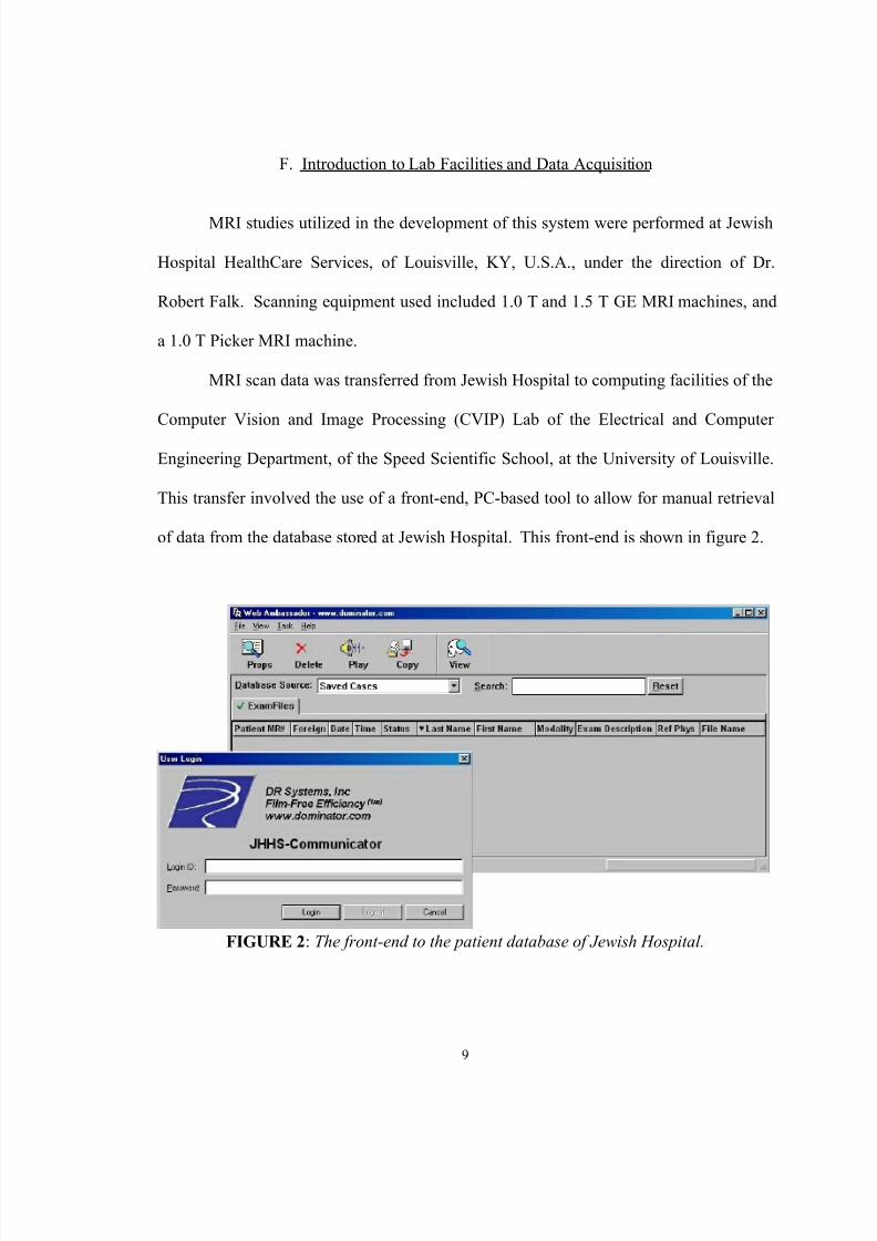
F. Introduction to Lab Facilities and Data Acquisition
MRI studies utilized in the development of this system were performed at Jewish
Hospital HealthCare Services, of Louisville, KY, U.S.A., under the direction of Dr.
Robert Falk. Scanning equipment used included 1.0 T and 1.5 T GE MRI machines, and
a 1.0 T Picker MRI machine.
MRI scan data was transferred from Jewish Hospital to computing facilities of the
Computer Vision and Image Processing (CVIP) Lab of the Electrical and Computer
Engineering Department, of the Speed Scientific School, at the University of Louisville.
This transfer involved the use of a front-end, PC-based tool to allow for manual retrieval
of data from the database stored at Jewish Hospital. This front-end is shown in figure 2.
FIGURE 2 : The front-end to the patient database of Jewish Hospital.
8/12/2019 Jeremy Nett
http://slidepdf.com/reader/full/jeremy-nett 25/124
10
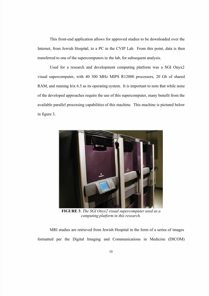
This front-end application allows for approved studies to be downloaded over the
Internet, from Jewish Hospital, to a PC in the CVIP Lab. From this point, data is then
transferred to one of the supercomputers in the lab, for subsequent analysis.
Used for a research and development computing platform was a SGI Onyx2
visual supercomputer, with 40 300 MHz MIPS R12000 processors, 20 Gb of shared
RAM, and running Irix 6.5 as its operating system. It is important to note that while none
of the developed approaches require the use of this supercomputer, many benefit from the
available parallel processing capabilities of this machine. This machine is pictured below
in figure 3.
FIGURE 3 : The SGI Onyx2 visual supercomputer used as acomputing platform in this research.
MRI studies are retrieved from Jewish Hospital in the form of a series of images
formatted per the Digital Imaging and Communications in Medicine (DICOM)
8/12/2019 Jeremy Nett
http://slidepdf.com/reader/full/jeremy-nett 26/124
11
specification of the American College of Radiology (ACR) and National Electrical
Manufacturers Association (NEMA) [42]. Each image from a study is in a separate file.
The images are extracted from the DICOM files and formatted for use, including
necessary scaling. Additionally, necessary parameters from the DICOM header (such as
pixel sizes, slice thickness, etc.) are read and recorded for use.
G. Outline of the Components of the Researched Solution
The approaches taken in this research address two fronts of the study of multiple
sclerosis using MRI studies, image processing techniques, and visualization: quantitative
evaluation of disease burden via the use of segmentation and classification techniques,
and qualitative evaluation via the use of volume registration and visualization paradigms.
Segmentation and classification techniques from the fields of pattern recognition
and image processing are applied for segmentation of the brain from the head of a patient,
followed by classification of the extracted volume into CSF, normal brain material, and
diseased brain tissue. Emphasis is placed upon automation of these steps, using computer
vision tools, to allow for timely assessment of a large number of MRI studies, and for
objective, repeatable measurement of disease burden from MR images. From a
segmentation of normal brain material and diseased tissue, quantification of disease
burden may be evaluated by computation of the normal and diseased brain volumes of a
patient.
Qualitative evaluation of the disease burden of a patient is important to allow for
evaluation of disease pathology interactively by an expert, and to allow for judgment of
8/12/2019 Jeremy Nett
http://slidepdf.com/reader/full/jeremy-nett 27/124
12
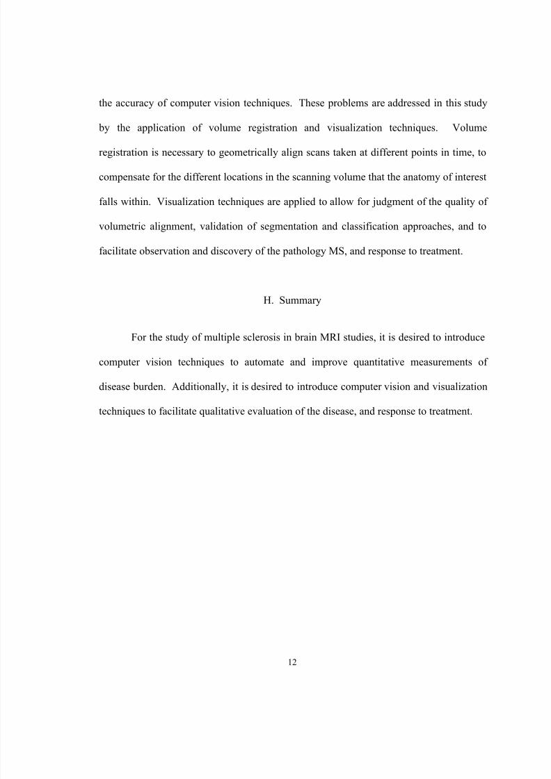
the accuracy of computer vision techniques. These problems are addressed in this study
by the application of volume registration and visualization techniques. Volume
registration is necessary to geometrically align scans taken at different points in time, to
compensate for the different locations in the scanning volume that the anatomy of interest
falls within. Visualization techniques are applied to allow for judgment of the quality of
volumetric alignment, validation of segmentation and classification approaches, and to
facilitate observation and discovery of the pathology MS, and response to treatment.
H. Summary
For the study of multiple sclerosis in brain MRI studies, it is desired to introduce
computer vision techniques to automate and improve quantitative measurements of
disease burden. Additionally, it is desired to introduce computer vision and visualization
techniques to facilitate qualitative evaluation of the disease, and response to treatment.
8/12/2019 Jeremy Nett
http://slidepdf.com/reader/full/jeremy-nett 28/124
13
II. VOLUME REGISTRATION
A. Introduction to Volume Registration
Typically in an MRI study, a patient is placed in the scanner with little regard for
positioning of the anatomy of interest. The only constraints are that the anatomy of
interest falls within the scanning volume, and that the patient is generally placed in some
orientation such that gross anatomical features are placed in some direction (for example,
the patient's nose points upward in the scanner).
In the context of qualitative evaluation of MS studies however, this arrangement
leads to hindrances in evaluation, due to the fact that multiple scans must be compared
with one another. Due to the largely arbitrary positioning of the anatomy in the scanner,
in a slice-by-slice comparison between studies, quite different anatomy can by chance be
located on the same slice numbers in different studies. The goal of registration, therefore,
is to align the anatomy from one scan, to the anatomy from a second. When this function
is performed, the resulting volumes are said to be registered; without this function, the
volumes are said to be mis-registered.
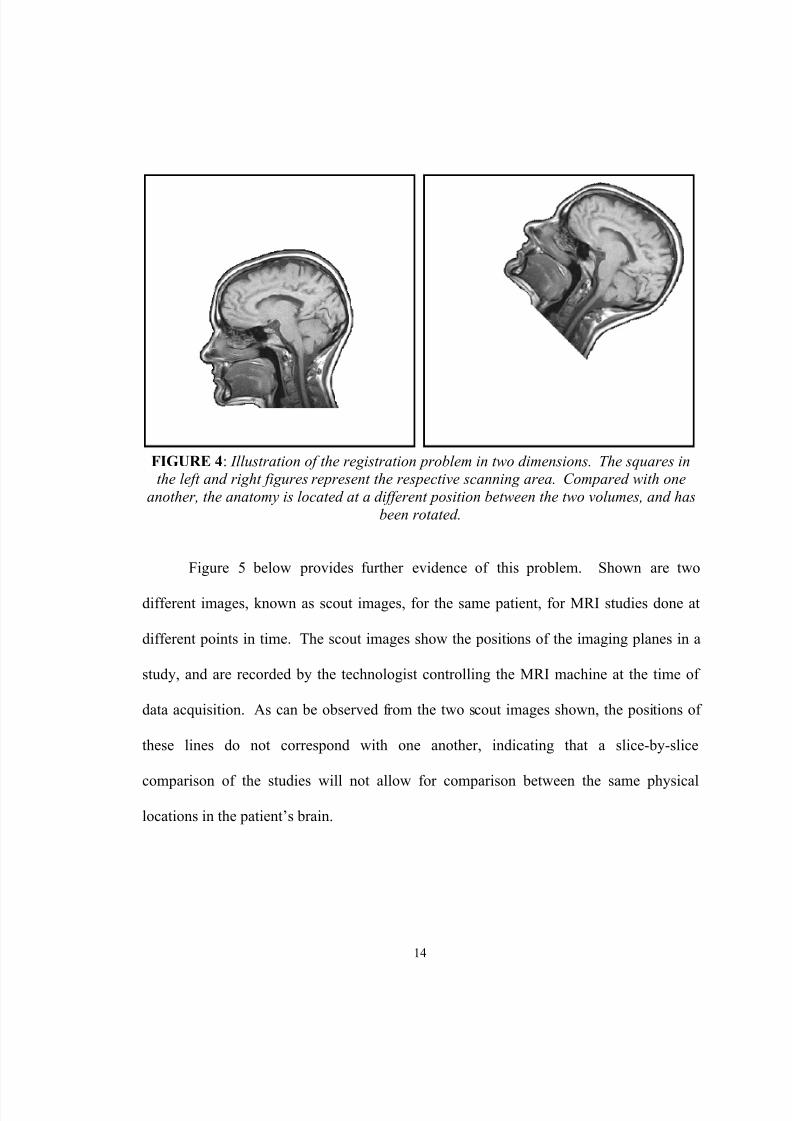
Figure 4 below illustrates the problem of mis-registration in two dimensions.
Here, the box represents a scanning area. Comparing the positioning of the anatomy in
the left and right scanning areas, the volumes are out of alignment by three factors: two
translation quantities (a horizontal and vertical), and a rotation angle. Registration is the
function by which these quantities are discovered or calculated, thereby supplying the
information necessary to relate one volume to another, in the sense of alignment.
8/12/2019 Jeremy Nett
http://slidepdf.com/reader/full/jeremy-nett 29/124
14
FIGURE 4 : Illustration of the registration problem in two dimensions. The squares inthe left and right figures represent the respective scanning area. Compared with one
another, the anatomy is located at a different position between the two volumes, and hasbeen rotated.
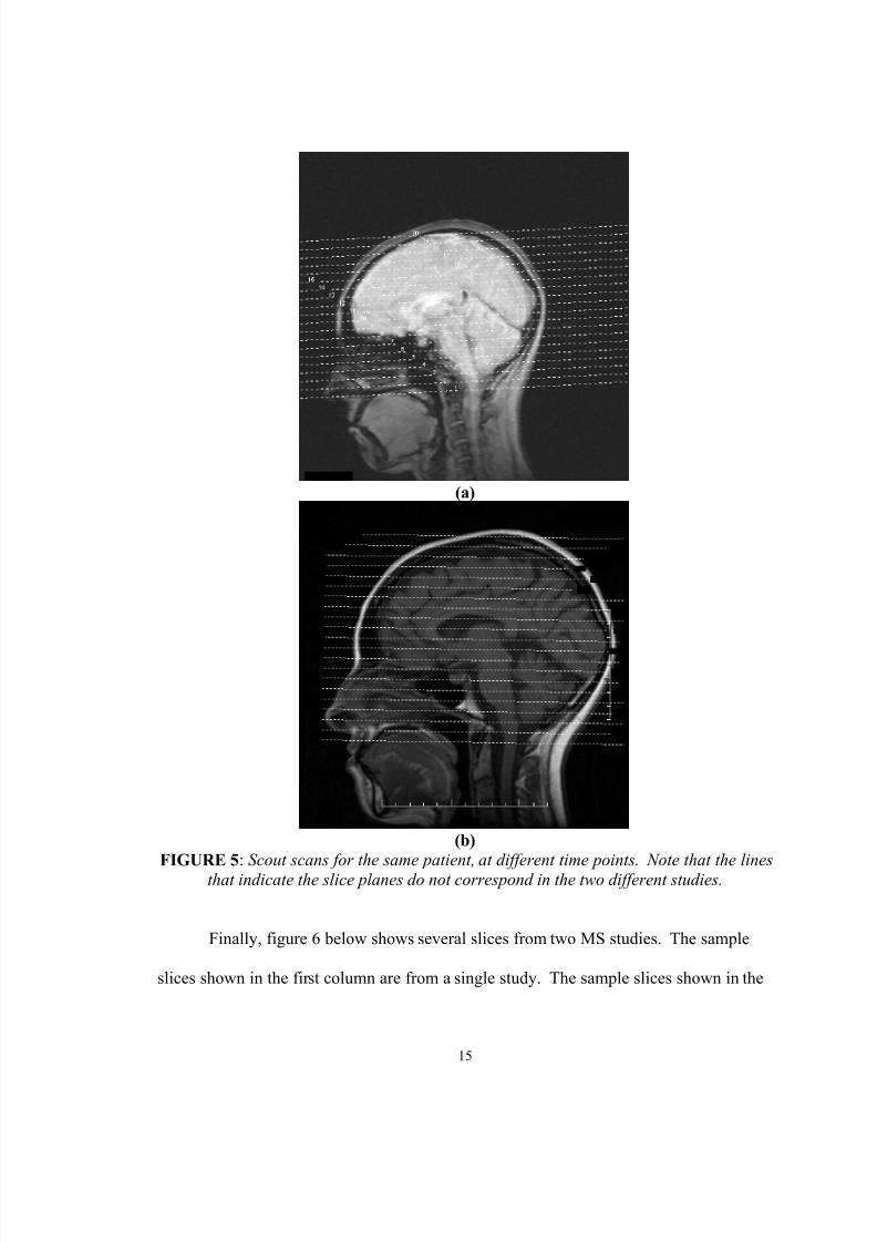
Figure 5 below provides further evidence of this problem. Shown are two
different images, known as scout images, for the same patient, for MRI studies done at
different points in time. The scout images show the positions of the imaging planes in a
study, and are recorded by the technologist controlling the MRI machine at the time of
data acquisition. As can be observed from the two scout images shown, the positions of
these lines do not correspond with one another, indicating that a slice-by-slice
comparison of the studies will not allow for comparison between the same physical
locations in the patient’s brain.
8/12/2019 Jeremy Nett
http://slidepdf.com/reader/full/jeremy-nett 30/124
15
(a)
(b)FIGURE 5 : Scout scans for the same patient, at different time points. Note that the lines
that indicate the slice planes do not correspond in the two different studies.
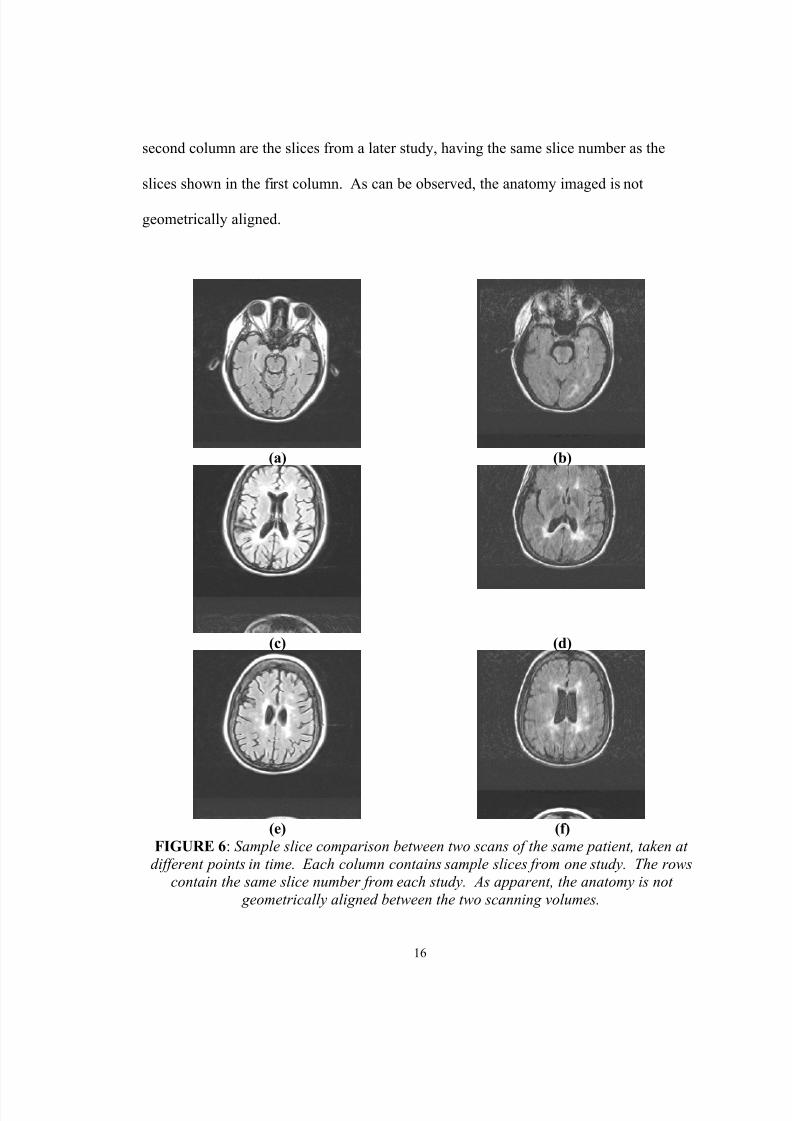
Finally, figure 6 below shows several slices from two MS studies. The sample
slices shown in the first column are from a single study. The sample slices shown in the
8/12/2019 Jeremy Nett
http://slidepdf.com/reader/full/jeremy-nett 31/124
16
second column are the slices from a later study, having the same slice number as the
slices shown in the first column. As can be observed, the anatomy imaged is not
geometrically aligned.
(a) (b)
(c) (d)
(e) (f)FIGURE 6 : Sample slice comparison between two scans of the same patient, taken at
different points in time. Each column contains sample slices from one study. The rowscontain the same slice number from each study. As apparent, the anatomy is not
geometrically aligned between the two scanning volumes.
8/12/2019 Jeremy Nett
http://slidepdf.com/reader/full/jeremy-nett 32/124
17
Registration is a crucial problem to be addressed in many medical imaging tasks,
and can be useful for facilitating a comparison between two or more studies of a patient,
merging two or more imaging modalities to facilitate diagnosis, and even to aid in
segmentation.
It is desirable to be able to perform registration using computer vision approaches,
rather than imposing limitations in the scanning procedure, or affixing artificial fiducial
markers on the patient’s head. For best accuracy, artificial markers would likely be
affixed to the skull, and therefore would be inconvenient and potentially painful for the
patient. Additionally, this procedure would also introduce a risk of infection.
Furthermore, using computer vision techniques, it is also desirable to be able to apply
registration retroactively, allowing for current data sets to be aligned with data sets taken
previously in a patient’s history, or perhaps with an imaging modality that prevents the
use of artificial markers.
In the study of MS using MRI, for comparison of scans taken at different points of
time in a clinical study, of the same patient, a registration technique is necessary. Such a
tool would allow for alignment of patient anatomy in the different scans. When this
alignment is accomplished, qualitative comparison of scans becomes easier to an expert
viewer, as image slices will now contain the same anatomy, and quantitative comparison
between studies is enabled in the same manner.
Registration can also be used to assist in segmentation. For example, if a model
of patient anatomy is known, then a study can be registered to that model, allowing for
segmentation of certain classes of problems to be made trivial, as the segmentation of the
8/12/2019 Jeremy Nett
http://slidepdf.com/reader/full/jeremy-nett 33/124
18
data set is then known a priori from the model. In this research, this approach is used for
segmentation of a patient’s brain from his head, and is discussed in detail in later portions
of this thesis.
In this context, a well-known and useful volume registration technique, known as
registration by maximization of mutual information, was investigated [14, 15]. This
technique has generally been found to perform well, and is useful in clinical settings [16].
This technique was studied, implemented, and tested using MS patient studies.
Additionally, the performance of this method was enhanced by application of parallel
programming techniques.
Below, this technique, implementation, and parallelization will be discussed.
First, an imaging model will be described, by which data from an imaging study is
modeled in three-dimensional space. Secondly, the types of transformations between two
volumes that are useful in this context will be addressed. Thirdly, volume registration
using computer vision, and specifically, the criterion of mutual information, shall be of
concern. Then, the application of this criterion to the problem of volume registration will
be expounded upon, followed by the application of parallel programming techniques to
improve the performance of the software implementation of this registration technique.
Lastly, results obtained using this method are shown, for MS studies using MRI.
8/12/2019 Jeremy Nett
http://slidepdf.com/reader/full/jeremy-nett 34/124
19
B. Imaging Model
Of preliminary concern is the construction of a volume from an imaging study,
and modeling the relationship of this volume to three-dimensional space.
Data obtained from an imaging study such as an MRI-based modality, or
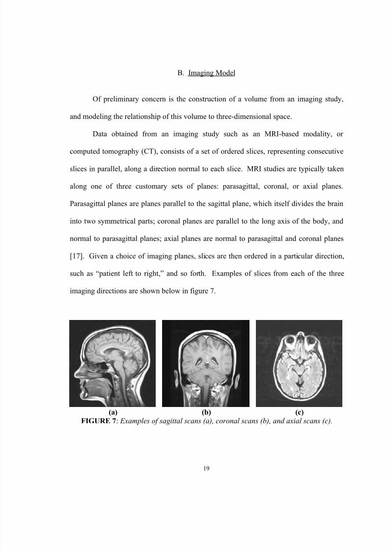
computed tomography (CT), consists of a set of ordered slices, representing consecutive
slices in parallel, along a direction normal to each slice. MRI studies are typically taken
along one of three customary sets of planes: parasagittal, coronal, or axial planes.
Parasagittal planes are planes parallel to the sagittal plane, which itself divides the brain
into two symmetrical parts; coronal planes are parallel to the long axis of the body, and
normal to parasagittal planes; axial planes are normal to parasagittal and coronal planes
[17]. Given a choice of imaging planes, slices are then ordered in a particular direction,
such as “patient left to right,” and so forth. Examples of slices from each of the three
imaging directions are shown below in figure 7.
(a) (b) (c)FIGURE 7 : Examples of sagittal scans (a), coronal scans (b), and axial scans (c).
8/12/2019 Jeremy Nett
http://slidepdf.com/reader/full/jeremy-nett 35/124
20
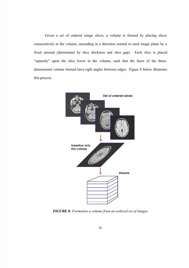
Given a set of ordered image slices, a volume is formed by placing slices
consecutively in the volume, ascending in a direction normal to each image plane by a
fixed amount (determined by slice thickness and slice gap). Each slice is placed
“squarely” upon the slice lower in the volume, such that the faces of the three-
dimensional volume formed have right angles between edges. Figure 8 below illustrates
this process.
FIGURE 8 : Formation a volume from an ordered set of images
8/12/2019 Jeremy Nett
http://slidepdf.com/reader/full/jeremy-nett 36/124
21
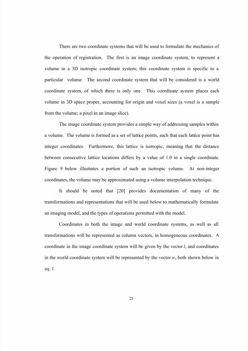
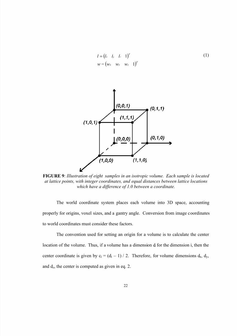
There are two coordinate systems that will be used to formulate the mechanics of
the operation of registration. The first is an image coordinate system, to represent a
volume in a 3D isotropic coordinate system; this coordinate system is specific to a
particular volume. The second coordinate system that will be considered is a world
coordinate system, of which there is only one. This coordinate system places each
volume in 3D space proper, accounting for origin and voxel sizes (a voxel is a sample
from the volume; a pixel in an image slice).
The image coordinate system provides a simple way of addressing samples within
a volume. The volume is formed as a set of lattice points, such that each lattice point has
integer coordinates. Furthermore, this lattice is isotropic, meaning that the distance
between consecutive lattice locations differs by a value of 1.0 in a single coordinate.
Figure 9 below illustrates a portion of such an isotropic volume. At non-integer
coordinates, the volume may be approximated using a volume interpolation technique.
It should be noted that [20] provides documentation of many of the
transformations and representations that will be used below to mathematically formulate
an imaging model, and the types of operations permitted with the model.
Coordinates in both the image and world coordinate systems, as well as all
transformations will be represented as column vectors, in homogeneous coordinates. A
coordinate in the image coordinate system will be given by the vector l , and coordinates
in the world coordinate system will be represented by the vector w, both shown below in
eq. 1.
8/12/2019 Jeremy Nett
http://slidepdf.com/reader/full/jeremy-nett 37/124
22
( )( )T z y x
T z y x
wwww
l l l l
1
1
==
(1)
FIGURE 9 : Illustration of eight samples in an isotropic volume. Each sample is locatedat lattice points, with integer coordinates, and equal distances between lattice locations
which have a difference of 1.0 between a coordinate.
The world coordinate system places each volume into 3D space, accounting
properly for origins, voxel sizes, and a gantry angle. Conversion from image coordinates
to world coordinates must consider these factors.
The convention used for setting an origin for a volume is to calculate the center
location of the volume. Thus, if a volume has a dimension d i for the dimension i, then the
center coordinate is given by c i = (d i – 1) / 2. Therefore, for volume dimensions d x, dy,
and d z, the center is computed as given in eq. 2.

8/12/2019 Jeremy Nett
http://slidepdf.com/reader/full/jeremy-nett 38/124
23
T z y x
d d d d c −−−=−= 12 12 12 12 1 (2)
Incorporation of the volume center as an origin for locating the volume in 3D
space is given by multiplication of the image coordinate vector l by the matrix C, given in
eq. 3.
−−−
=
1000
100
010
001
z
y
x
c
c
c
C
(3)
Voxel sizes are the spatial sampling periods of the imaged volume. There are
three such sizes, v x, v y, and v z, representing the size of a voxel in each of the coordinate
dimensions. Incorporation of the voxel sizes in proper scaling of the image coordinates
to world coordinates is given by multiplication of the image coordinate vector l by the
matrix V, given below in eq. 4.

8/12/2019 Jeremy Nett
http://slidepdf.com/reader/full/jeremy-nett 39/124
24
=
1000000
000
000
z
y
x
v
v
v
V
(4)
Finally, an additional term, a gantry angle γ, is taken into consideration. This
term measures the angle of the gantry as it is positioned in the scanner. This factor is
easily incorporated in conversion of an image coordinate vector l to world coordinates by
the matrix Γ, given below in eq. 5. Note that this matrix is simply a rotation matrix, a
class of transformations to be discussed further below.
=Γ
1000
01sin000cos0
0001
γγ
(5)
Therefore, with each of these matrices considered, the conversion from image to
world coordinates can be represented as the matrix product of the Γ, V , and C matrices.
The resulting coordinate transformation is referenced as A i,w , and is given below in eq. 6.

8/12/2019 Jeremy Nett
http://slidepdf.com/reader/full/jeremy-nett 40/124
25
⋅⋅−⋅−⋅
⋅⋅−⋅
⋅−
=⋅⋅Γ=
1000sinsin0
cos0cos0
00
,
γγ
γγ y y z z y
y y y
x x x
wi
cvcvvz v
cvv
cvv
C V A
(6)
It will be of interest to be able to convert from world coordinates into image
coordinates. This can be simply done by inverting the A i,w matrix, to obtain A i,w-1, as
given in eq. 7 below, in closed form.
⋅
−⋅=−
1000
1
cos
sin0
0cos1
0
001
1,
z
z z
y y
x x
wi
cvv
cv
cv
A
γ
γγ
(7)
Thus, the relationships given in eq. 8 allow for conversion between image and
world coordinates.
w Al
l Aw
wi
wi
⋅=⋅=
−1,
,
(8)
8/12/2019 Jeremy Nett
http://slidepdf.com/reader/full/jeremy-nett 41/124
26
Each of the above parameters (d x, dy, dz, vx, vy, vz, γ) are known a priori
parameters obtained from the DICOM header of a study.
Two volumes will be used in the registration, a reference volume R, and a floating
volume F. The purpose of registration is to find a transformation that aligns these two
volumes.
C. Transformations
For alignment, rotation and translation will be considered. Alignment
transformations that consist of only translation and rotation are known as rigid-body
transformations.
Only the translation and rotation transformations are considered here, as these
effects are observed in the data to be by far the predominant effects necessary for
registration of two or more studies of the same patient. Other transformations are judged
to be either negligible in effect, or not applicable. Included in these transformations are
scaling (or magnification) between two studies, as the voxel sizes (the metric dimensions
of a voxel) of each study are known from the scanner, and are known to be accurate
enough for use, given that the scanner is in good repair.
Translation quantifies a three-dimensional offset along coordinate axes between
two volumes in world coordinates. In homogeneous coordinates, with t x, ty, and t z
representing translation along the x, y, and z coordinate axes, respectively, the translation

8/12/2019 Jeremy Nett
http://slidepdf.com/reader/full/jeremy-nett 42/124
27
can be formulated by a matrix T, that multiplies a coordinate w to obtain a translated
coordinate vector. T is given below in eq. 9.
=
1000
100
010
001
z
y
x
t
t
t
T
(9)
A rotation is quantified by three angles, φx, φy, φz, that are axis-angle
parameterizations of rotation. These parameters specify a rotation around the unit
direction vectors of the world coordinate system. Corresponding to each parameter is a
rotation matrix, denoted as R x, R y, and R z, respectively. A complete rotation matrix,
taking into account each rotation angle, is given by the matrix product of R x, R y, and R z,
and forms the matrix R, given in eq. 13 below. R x, R y, and R z are given in eqs. 10
through 12, respectively.
−=
1000
0cossin0
0sincos0
0001
x x
x x x R φφ
φφ
(10)

8/12/2019 Jeremy Nett
http://slidepdf.com/reader/full/jeremy-nett 43/124
28
−
=
10000cos0sin
0010
0sin0cos
y y
y y
y Rφφ
φφ
(11)
−=
1000
0100
00cossin
00sincos
z z
z z
z Rφφφφ
(12)
Rz Ry Rx R ⋅⋅= (13)
Utilization of the matrices T and R constitutes a rigid-body transformation. The
complete transformation can be written as the product of these two matrices, and shall be
denoted as A . To calculate the rigid body transformation of a coordinate w, the
coordinate vector w is multiplied by the transformation matrix A , as shown in eq. 14,
where w1 is a coordinate, and w2 is the rigid body transformation of that coordinate.
12 w Aw ⋅= (14)

8/12/2019 Jeremy Nett
http://slidepdf.com/reader/full/jeremy-nett 44/124
29
Next, a formulation of the above rigid body transformation shall be given. Below,
wF, l F, wR , and l R will represent world and image coordinates in the floating volume, and
world and image coordinates in the reference volume, respectively. A i,w,F and A i,w,R will
represent the transformations from image to world coordinates for the floating and
reference volumes, respectively. The matrix A represents the transformation between
two volumes, as a function of the registration parameters. A FR will represent the
transformation between the floating and reference volume, in the image coordinate
system of each volume.
The below formation is a simple derivation based on eqs. 6, 7, 8, and 14.
Essentially, by taking the transformation between world coordinates, given by eq. 14, and
the relationships between image and world coordinates given by eqs. 6 through 8, eq. 15
below can be written.
( ) F FR R
F F wi Rwi R
F F wi R Rwi
F R
wT l
wT AT l
wT Al T
w Aw
×=×××=
××=×⋅=
−,,
1,,
,,,,
(15)
Therefore, using the results given in eq. 15, computation of the matrix T FR allows
only coordinates in the image to be dealt with explicitly.
8/12/2019 Jeremy Nett
http://slidepdf.com/reader/full/jeremy-nett 45/124

8/12/2019 Jeremy Nett
http://slidepdf.com/reader/full/jeremy-nett 46/124
31
TABLE ISAMPLES AND SAMPLE WEIGHTINGS FOR TRILINEAR INTERPOLATION.
3 _ _
2 _ _
1 _ _
N left lower z delta
N left lower ydelta
N left lower xdelta
Z
Y
X
−=−=−=
Z Y X
Z Y X
Z Y X
Z Y X
Z Y X
Z Y X
Z Y X
Z Y X
deltadeltadeltaweight
deltadeltadeltaweight deltadeltadeltaweight
deltadeltadeltaweight
deltadeltadeltaweight
deltadeltadeltaweigth
deltadeltadeltaweight
deltadeltadeltaweight
∗∗=∗∗−=∗−∗=
∗−∗−=−∗∗=
−∗∗−=−∗−∗=
−∗−∗−=
7
6
5
4
3
2
1
0
)1()1(
)1()1(
)1(
)1()1(
)1()1(
)1()1()1(
)13 _ _ ,12 _ _ ,11 _ _ (
)13 _ _ ,12 _ _ ,1 _ _ (
)13 _ _ ,2 _ _ ,11 _ _ (
)13 _ _ ,2 _ _ ,1 _ _ (
)3 _ _ ,12 _ _ ,11 _ _ (
)3 _ _ ,12 _ _ ,1 _ _ (
)3 _ _ ,2 _ _ ,11 _ _ (
)3 _ _ ,2 _ _ ,1 _ _ (
7
6
5
4
3
2
1
0
+++=++=++=
+=++=
+=+=
=
N left lower N left lower N left lower sample
N left lower N left lower N left lower sample
N left lower N left lower N left lower sample
N left lower N left lower N left lower sample
N left lower N left lower N left lower sample
N left lower N left lower N left lower sample
N left lower N left lower N left lower sample
N left lower N left lower N left lower sample
interpolated_value = ∑=
∗7
0
)(i
ii sampleV weight
E. Overview of Registration Approaches
Computer-assisted registration has received a large amount of attention in
medical imaging, owing to its importance, and the strong desire for an automated, non-
invasive approach. Consequently, there are a number of different paradigms that have
8/12/2019 Jeremy Nett
http://slidepdf.com/reader/full/jeremy-nett 47/124
32
been introduced for 3D volume registration, including landmark-based methods,
segmentation-based methods, surface-based methods, and volumetric methods [18, 19].
In this work, registration is pursued using a technique based on volumetric
registration. The choice of this approach allows for the features used for registration to
be the samples comprising the volumes to be registered directly, with no pre-processing
or feature extraction applied. This technique, known as volume registration by
maximization of mutual information, relies on the evaluation of a metric function to
quantify the quality of alignment, of the floating and reference volumes, given a
registration parameter vector. The metric function used is the mutual information
function of the floating and reference volumes.
F. Registration Metric/Criteria
Relative entropy, also known as the Kullbak Leibler distance, between two
probability mass functions p(x) and q(x), is defined as the quantity D(p||q), given in eq.
16 below [21].
∑ ⋅= X xq x p
x pq p D )()(
log)()||( 2 (16)
8/12/2019 Jeremy Nett
http://slidepdf.com/reader/full/jeremy-nett 48/124
33
For two discrete random variables X and Y, with marginal probability mass
functions p X(x) and p Y(y), and a joint distribution p(x, y), the mutual information
function I(x,y) is the relative entropy between the joint distribution p(x, y), and the
distribution p X(x)•p Y(y), the joint distribution when X and Y are independent random
variables. Thus, the mutual information of X and Y is given in eq. 17 below [17].
∑⋅
⋅=⋅=Y X Y X
Y X y p x p y x p y x p y p x p y x p DY X I
,2 )()(
),(log),())()(||),((),( (17)
If X and Y are independent random variables, then p(x, y) is given by the product
of the marginals p X(x) and p Y(y), and therefore, the quantity that is the argument of the
logarithm function in eq. 17 is one. As the logarithm of one is zero, the mutualinformation I(X, Y), when X and Y are statistically independent, is zero.
There is a close relationship between entropy, a measure of information content,
and the mutual information quantity. The entropy H(X) of a discrete random variable X
is defined in eq. 18. The joint entropy H(X,Y) of the discrete random variables X and Y
is defined below in eq. 19. The conditional entropy H(Y|X) of the discrete random
variables X and Y is defined below in eq. 20 [21].

8/12/2019 Jeremy Nett
http://slidepdf.com/reader/full/jeremy-nett 49/124
34
∑ ⋅−= X
x p x p X H )(log)()( 2 (18)
∑ ⋅−=Y X
y x p y x pY X H ,
2 ),(log),(),( (19)
∑ ⋅−=Y X
x y p y x p X Y H ,
2 )|(log),()|( (20)
Entropy is a common measurement of information content. Information content
is increased as entropy is increased, and decreased as entropy is decreased. The less
concentrated a probability density or mass function is, the more information content that
is encoded in the random variable. For example, consider a continuous random variable
X. If X is distributed as a uniform random variable, the information content of X is
greatest, because over the range of X, the probability of X taking on a value x 1 is equal in
all cases to X taking on a value of x 2. For X distributed as a Gaussian random variable,
with a mean µ and variance σ2, X encodes less information, as the values of X around µ
are more likely than values far from µ, with the spread or concentration of probability
around µ quantified by the variance σ2.
By simple algebraic manipulation, and using the definition of conditional
probabilities, the mutual information function I(X,Y) can be related in a number of ways
to the entropy quantities given in eqs. 18 through 20. These relationships are given
below in eqs. 21 and 22.
8/12/2019 Jeremy Nett
http://slidepdf.com/reader/full/jeremy-nett 50/124
8/12/2019 Jeremy Nett
http://slidepdf.com/reader/full/jeremy-nett 51/124
36
),()()(),( F T R H F T H R H F T R I ααα −+= (25)
In the process of registration, only the overlapping portions of the reference and
transformed floating volumes will be considered in computation of the mutual
information metric, as will be discussed below. Therefore, the quantities H(R) and
H(T αF) change little, over the range of registration parameters considered.
Considering the relationship between the mutual information metric and entropy
given in eq. 24, then, it can be observed that maximization of I(R, T αF) is equivalent to
minimization of H(R|T αF). Thus, by minimization of H(R|T αF), given T αF, the
information content of R is to be minimized. Qualitatively, if T αF is known, then the
information measure H(R|T αF) is low, as minimization of I(R, T αF) has established a
relationship between the observations of R, and the observations of T αF, regardless of the
mathematical nature of the relationship. This property allows the mutual information
metric to be useful for multimodal registration, where other similarity metrics perform
poorly [22].
Considering the relationship between the mutual information metric and entropy
given in eq. 25, it can be observed that maximization of I(R, T αF) is equivalent to
minimization of H(R, T αF). Thus, by minimization of H(R, T αF), the information content
of (R, T αF) is minimized. In terms of the joint probability mass function p(r, T αf), this
corresponds to building concentrations of probability, as observed in a comparison
information content of a random variable distributed as a Gaussian to a random variable
distributed uniformly. This process allows for registration by favoring registration
8/12/2019 Jeremy Nett
http://slidepdf.com/reader/full/jeremy-nett 52/124
37
parameters that establish a relationship between the reference and floating volumes, with
this relationship being the spatial alignment of anatomy, implicitly.
G. Computation of the Mutual Information Metric
Computation of the mutual information metric is based upon direct evaluation of
eq. 23. Furthermore, this computation is improved in terms of execution speed on the
Onyx2 supercomputer by dividing the task of computation of I(R, T αF) across several
processors. Computation of the metric, and parallelization of this computation is
discussed below.
Beginning with computation of the metric, from eq. 23, three quantities are
necessary: p(r, T αf), p R (r), and p TαF(Tαf). The marginals p R (r) and p TαF(Tαf) may be
obtained directly from the joint probability function p(r, T αf). The joint probability mass
function p(r, T αf) will be approximated by the normalized joint histogram h(r, T αf). Here,
normalization refers to scaling of the histogram, such that the sum of approximated
probabilities equals 1.0. The marginals are then approximated from h(r, T αf) by
summation over the rows of h(r, T αf), and then the columns.
Computation of h(r, T αf) involves a complete iteration over each sample in the
floating volume. For each sample, the transformation T α is applied, to arrive at a
coordinate set in the image coordinate system of the reference volume. If the
transformed coordinate is outside the measured reference volume, then the remaining
operations are not executed, and the process starts again with the next sample in the
floating volume. Otherwise, a sample in the reference volume at the transformed
8/12/2019 Jeremy Nett
http://slidepdf.com/reader/full/jeremy-nett 53/124
38
coordinates is approximated using trilinear interpolation, and discretized. The two
samples, one from the floating volume, and one from the reference volume, are then
binned in the joint histogram.
In the studies considered here, each sample obtained from the MRI is an 8-bit
sample, allowing for 256 discrete levels. In the computation of the joint histogram
h(r,T αf), each discrete level is utilized in the joint and marginal histograms. Therefore,
there are 256 x 256 = 65,536 bins in the joint histogram, and 256 each in the marginal
histograms.
Computation of the joint histogram involves the processing of each sample in the
floating volume, application of a transformation to the coordinate of the sample in the
floating volume to obtain a coordinate in the reference volume, interpolation in the
reference volume, and binning in the joint histogram. For a typical 256 x 256 x 20 MRI
volume, there are thus 256 x 256 x 20 = 1,310,720 samples to process.
Following computation of the joint histogram, normalization and computation of
the marginal histograms must be performed. This involves one pass over the joint
histogram, therefore processing 256 x 256 = 65,536 elements from the joint histogram.
This processing consists of normalization, and summation to compute the marginal
histograms.
Following this operation, the mutual information metric itself may be computed.
This processing involves computation of the sum given eq. 23, and involves one pass
over the joint histogram, therefore processing 256 x 256 = 65,536 elements that compose
the sum given in eq. 23.
8/12/2019 Jeremy Nett
http://slidepdf.com/reader/full/jeremy-nett 54/124
39
Therefore, computation of the joint histogram is by far the most computationally
costly component in computation of the mutual information metric. Therefore,
performance may be best increased by decreasing the execution time of the computation
of the joint histogram. Computation of the joint histogram is an amenable problem for
parallel execution, as computation of a part of the joint histogram does not depend on the
computational results of any other part of the joint histogram, allowing individual bins, or
entire regions of the joint histogram to be computed independently, and then merged to
form the total joint histogram.
The architecture of the SGI Onyx2 supercomputer allows for tasks running on
different processors to access memory anywhere within the 20 Gb of shared memory in
the machine. Reads from an arbitrary location in memory, then, are unfettered. Writes to
memory, however, should be carefully planned, so as to avoid potential problems with
performance decreases, due to cache refreshes. Therefore, a desired parallel solution
should permit reading of common input data from only one location (to avoid
unnecessary duplication and other overhead), but also keep outputs of the computation
local to a process.
For implementation of parallel execution, POSIX pthreads are used. The
implementation on the SGI Onyx2 allows for full utilization of the shared memory
capabilities of the machine. Furthermore, the use of POSIX pthreads allows for the
developed application to be easily ported to other architectures and operating systems,
such as a personal computer (PC) running a variant of the Linux operating system.

8/12/2019 Jeremy Nett
http://slidepdf.com/reader/full/jeremy-nett 55/124
40
A solution to this problem, fitting within the above constraints, is a division of the
computation of the joint histogram into two tasks. The first task computes a number of
joint histograms over sub-volumes. The second task merges these sub-joint histograms to
form the total joint histogram. Below, figure 10 illustrates the architecture of the
solution.
8/12/2019 Jeremy Nett
http://slidepdf.com/reader/full/jeremy-nett 56/124
41
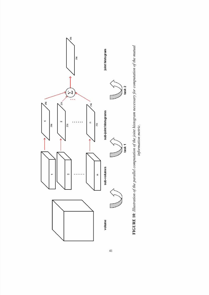
F I G U R E 1 0 : I l l u s t r a t i o n o f t h e p a r a l l e l c o m p u t a
t i o n o f t h e
j o i n t h i s t o g r a m n e c e s
s a r y f o r c o m p u t a t i o n o f t h e m u t u a l
i n f o r m a t i o n m e t r i c .
8/12/2019 Jeremy Nett
http://slidepdf.com/reader/full/jeremy-nett 57/124
42
Given a division of the floating volume into a set of sub-volumes, each process or
thread in task 1 computes a joint histogram over a sub-volume. Subsequent tasks cannot
proceed until all of the task 1 threads are finished in their execution, therefore, load
balancing between threads is accomplished by parameterizing the number of slices from
the floating volume to use per thread, and then by dynamic computation of the number of
threads that are necessary to execute. Each sub-joint histogram is computed as the joint
histogram is computed, as discussed above. The outputs of task 1 threads are a sub-joint
histogram corresponding to each sub-volume.
Given a set of sub-joint histograms, threads in task 2 compute the total joint
histogram over a region of the joint histogram. Each thread in task 2 has an assigned
region over which to compute the joint histogram. Given an element in the total joint
histogram to compute, the quantity is computed by summation over all sub-joint
histograms of the corresponding element. Load balancing between threads is
accomplished by dividing the total joint histogram into regions of equal numbers of
elements, and assigning a thread to compute a single region. The output of task 2 threads
is the total joint histogram.
Therefore, given a set of registration parameters, the mutual information metric
I(R,T αF) may be efficiently computed. As will be shown, this parallelization allows for
registration to be performed in an amount of time that is reasonable for the needs of the
proposed use as part of a study of the effectiveness of a multiple sclerosis treatment.
8/12/2019 Jeremy Nett
http://slidepdf.com/reader/full/jeremy-nett 58/124
43
H. Search Algorithm
The mutual information metric provides a quantitative measure of spatial
alignment between two volumes, given a choice of registration parameters. To obtain the
best alignment, it is necessary to maximize the metric. Maximization of the metric,
which is parameterized in terms of the registration parameters, is numerically
accomplished with the use of a search or maximization algorithm.
In the original formulation of registration by maximization of mutual information
in [14], Powell’s multidimensional optimization method, with Brent line minimizations
was used for maximization of the mutual information metric [23]. Subsequently, [24]
compares different classical optimization methods maximizing the mutual information
metric. One such method included in the study was the use of the classic Nelder and
Mead or simplex algorithm for maximization.
This method solely uses the objective function directly for optimization, and
therefore does not require the expensive computation of derivatives. This method is a
geometry-based method, using the geometric operations of contraction, expansion, and
reflection to manipulate a simplex to a maximum of the objective function. This method
was found to perform well in [24], and is utilized here for maximization of the mutual
information metric. The formulation implemented is derived from the presentation of the
algorithm in [23] and [25].
8/12/2019 Jeremy Nett
http://slidepdf.com/reader/full/jeremy-nett 59/124
44
I. Implementation
The implemented software for volume registration allows for volume registration
of two volumes with patient axes aligned a priori , over six registration parameters, which
include three translation quantities, and three rotation quantities, for 3D rigid-body
registration. The developed software tool utilizes parallel programming techniques to
obtain reasonable execution times. Output from the program includes the registration
parameters, and optionally, a re-sampled reference volume that is re-sampled along the
imaging planes of the floating volume.
The software was developed and tested on the SGI Onyx2 supercomputer, and
utilizes the parallel processing capabilities of this machine. The software, however, may
be ported to other architectures and operating systems with a trivial amount of effort, as
only standard, non-proprietary programming languages and libraries are used.
J. Results: MS studies
To assess the performance and accuracy of the implementation, the registration of
sample MS studies conducted at Jewish Hospital was performed. Data from five patients
(A, B, C, D, and E), and 7 studies were used. Table II below characterized the data sets
used, including specifications (imaging plane, weighting, dimensions, and voxel sizes) of
the reference and floating MRI studies.
8/12/2019 Jeremy Nett
http://slidepdf.com/reader/full/jeremy-nett 60/124
45
TABLE II PARAMETERS OF THE MS STUDIES USED FOR ASSESSING THE REGISTRATION
SOFTWARE DEVELOPED .
Reference Studystudy patient
date img.plane weighting dimensions voxel sizes (mm)
1 A 8/22/2001 axial FLAIR 256 x 256 x 21 0.937503 x 0.937500 x 5.02 B 7/27/2001 axial FLAIR 256 x 256 x 20 0.9375 x 0.9375 x 5.03 C 11/7/2000 axial FLAIR 256 x 256 x 20 0.9375 x 0.9375 x 5.04 A 8/22/2001 coronal T1 256 x 256 x 25 0.78125 x 0.78125 x 5.05 C 11/7/2000 sagittal T1 256 x 256 x 12 0.9375 x 0.9375 x 5.06 D 10/13/2001 axial FLAIR 256 x 256 x 21 0.937494 x 0.9375 x 5.07 E 3/27/1999 axial FLAIR 256 x 256 x 21 0.93749 x 0.9375 x 5.0
Floating Studydate img.
plane weighting dimensions voxel sizes (mm)
1 A 9/12/2000 axial FLAIR 256 x 256 x 20 0.9375 x 0.9375 x 5.02 B 1/29/2001 axial FLAIR 256 x 256 x 21 0.9375 x 0.9375 x 5.03 C 4/8/2000 axial FLAIR 256 x 256 x 20 0.9375 x 0.9375 x 5.04 A 9/12/2000 coronal T1 256 x 256 x 23 0.859375 x 0.859375 x 5.05 C 4/8/2000 sagittal T1 256 x 256 x 12 0.9375 x 0.9375 x 5.06 D 6/9/2000 axial FLAIR 256 x 256 x 20 0.9375 x 0.9375 x 5.07 E 11/3/2001 axial FLAIR 256 x 256 x 20 0.937496 x 0.9375 x 5.0
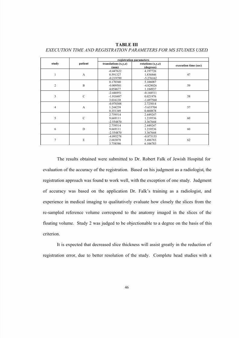
Table III below shows the registration parameters obtained, as well as the
execution time of the registration application. The registration parameters shown are the
six parameters comprising the parameter vector, including the three translation quantities
(tx, ty, and t z), and the three rotation angles ( φx, φy, and φz). The execution time shown
includes the entire execution time of the program, including initialization, the search for
the optimal registration parameters, and generation of a re-sampled output volume.
8/12/2019 Jeremy Nett
http://slidepdf.com/reader/full/jeremy-nett 61/124
46
TABLE III EXECUTION TIME AND REGISTRATION PARAMETERS FOR MS STUDIES USED .
registration parametersstudy patient translations (x,y,z)
(mm)rotations (x,y,z)
(degrees) execution time (sec)
1 A-0.4476220.591327-0.219799
4.1977261.836846-5.276162
47
2 B0.170340-0.0095014.054677
5.106087-4.8280261.184937
59
3 C-2.446951-1.9184873.016138
-0.1685110.021976-1.697560
58
4 A-0.9703081.2442390.351349
2.725014-5.6337040.460878
57
5 C
2.759514
9.669111-2.554870
2.449247
1.2195363.367644
60
6 D2.7595149.669111-2.554870
2.4492471.2195363.367644
60
7 E-4.0952782.6830783.758586
-0.8731555.4867836.106783
62
The results obtained were submitted to Dr. Robert Falk of Jewish Hospital for
evaluation of the accuracy of the registration. Based on his judgment as a radiologist, the
registration approach was found to work well, with the exception of one study. Judgment
of accuracy was based on the application Dr. Falk’s training as a radiologist, and
experience in medical imaging to qualitatively evaluate how closely the slices from the
re-sampled reference volume correspond to the anatomy imaged in the slices of the
floating volume. Study 2 was judged to be objectionable to a degree on the basis of this
criterion.
It is expected that decreased slice thickness will assist greatly in the reduction of
registration error, due to better resolution of the study. Complete head studies with a
8/12/2019 Jeremy Nett
http://slidepdf.com/reader/full/jeremy-nett 62/124
47
smaller slice thickness of MS patients were not available for use (the studies here all have
a slice thickness of 5.0 mm).
Validation of the registration results is a difficult problem. Direct evaluation of
the error in the registration parameters computed is not possible, as the actual registration
parameters are unknown. One possible way to quantify error is to have an expert
manually select corresponding points in the reference and floating volumes, and then to
calculate the registration between the selected, corresponding points. These registration
parameters would then be used as the actual registration parameters that may be
compared to the computed registration parameters for quantification of registration error.
This approach would introduce error in the manually selected points, however, nor was a
data set of corresponding points available for use here.
Figure 11 below shows sample slices from the registration studies. Each row of
the figure corresponds to a single study. The first column of the figure shows a sample
slice from the floating volume used for each study. The second column of the figure
shows the corresponding slice from the re-sampled reference volume. Finally, the third
column of the figure shows the checkerboard composite image formed by fusion of the
corresponding floating and re-sampled reference volume slices.
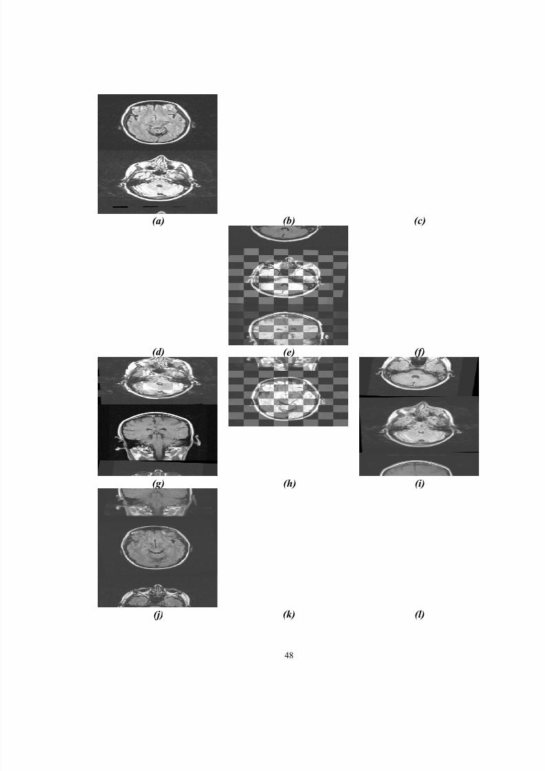
8/12/2019 Jeremy Nett
http://slidepdf.com/reader/full/jeremy-nett 63/124
48
(a) (b) (c)
(d) (e) (f)
(g) (h) (i)
(j) (k) (l)
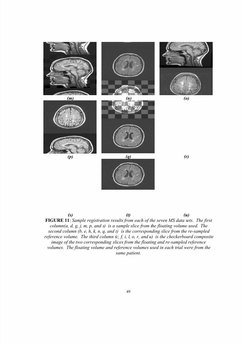
8/12/2019 Jeremy Nett
http://slidepdf.com/reader/full/jeremy-nett 64/124
49
(m) (n) (o)
(p) (q) (r)
(s) (t) (u)FIGURE 11 : Sample registration results from each of the seven MS data sets. The first
column(a, d, g, j, m, p, and s) is a sample slice from the floating volume used. The second column (b, e, h, k, n, q, and t) is the corresponding slice from the re-sampled
reference volume. The third column (c, f, i, l, o, r, and u) is the checkerboard compositeimage of the two corresponding slices from the floating and re-sampled reference
volumes. The floating volume and reference volumes used in each trial were from the same patient.
8/12/2019 Jeremy Nett
http://slidepdf.com/reader/full/jeremy-nett 65/124

8/12/2019 Jeremy Nett
http://slidepdf.com/reader/full/jeremy-nett 66/124
51
III. BRAIN SEGMENTATION FROM THE HEAD
A. Introduction and Necessity
Brain segmentation from the head refers to the process of extracting brain tissue
from the remaining tissues found in the head. Extracting the brain, including normal and
diseased tissue, as well as CSF, from the remaining tissues comprising the head, allows
for a simplified classifier to be applied for subsequent quantitative analysis of MS
lesions.
A Bayesian classifier is utilized for classification of normal and abnormal brain
tissue, and CSF. To this end, it is desirable to minimize the number of tissues that must
be modeled. The number of tissues that must be modeled, at minimum, is three: normal
brain tissue, abnormal brain tissue (MS lesions), and CSF. By removing other tissues,
such as eyes, skin, and fat, which are also imaged in an MRI study of the head, the
subsequent statistical classification can be simplified to the minimum number of tissues
that must be modeled. Removal of these extraneous tissue classes is accomplished here
with the use of a registration-based technique, to register a scan to a scan with a known
head segmentation.
Over several studies of an MS patient, it is not expected that the volume of the
brain will change appreciably. Changes in brain volume over time will be assumed to be
only due to brain atrophy, a reasonable assumption owing to the pathological nature of
MS [1,2,4]. As well, it is expected that if the obtained brain segmentation is slightly
8/12/2019 Jeremy Nett
http://slidepdf.com/reader/full/jeremy-nett 67/124
52
larger than the actual brain, this is acceptable, as CSF surrounds the brain, and a model
for CSF must be considered in any case.
Brain segmentation from the head, also known as “brain peeling,” has been
addressed by a number of research centers [26, 27, 28, 29]. These methods each claim at
least a degree of automation, and others, outright full automation. Reviewing these
studies, however, indicates that there is a large amount of data dependency of the method,
owing to choice of scan parameters. As the data sets here are simply provided, and were
acquired with scan parameters that benefited the radiologist, implementation of a
technique based on these studies is not pursued.
As it is assumed that a patient’s brain volume does not change dramatically, and
is limited to perhaps only brain atrophy, an approach to the segmentation of the brain
from the head is explored that is based upon registration, and utilizes the registration tool
developed during the course of this research.
B. Brain Segmentation Utilizing Registration
The underlying concept of registration-aided brain segmentation is that for a
patient, if an a priori segmentation is known, then registration of an arbitrary study
allows for the brain segmentation problem to be solved. This solution is trivial, as the
segmentation for the arbitrary volume is known from alignment of the study to the study
for which the segmentation is known. The known segmentation may then be applied to
the arbitrary study, achieving brain segmentation.

8/12/2019 Jeremy Nett
http://slidepdf.com/reader/full/jeremy-nett 68/124
53
For implementation of this approach, a rigid registration software tool, such as
developed for this study, must be available. Also, it is necessary to be able to generate a
brain segmentation from a patient, to serve as the a priori segmentation. This
segmentation may generally be manual, semi-automatic, or fully automatic. Here,
manual and semi-automatic methods [30] are explored for generation of the a priori
segmentation.
While undesirable in principle due to the need for human involvement, this
approach is acceptable for low numbers of patients, as only an initial brain segmentation
is necessary. As well, other factors related to human involvement, such as accuracy and
repeatability, are mitigated, as segmentation of the brain from the head is a gross
anatomical-recognition task. It is also acceptable if the segmentation includes additional
CSF surrounding the brain, and small errors in removing brain tissue should not be
appreciable with respect to the total volume of the brain, and given the spatial sampling
rates of the studies investigated.
A related approach would be to replace the a priori segmentation with a non-
patient specific head model, incorporating a known brain segmentation with the model.
Then, using non-rigid registration, an arbitrary patient study would be registered to the
model to provide for brain segmentation of the patient study. In this situation, the model
replaces the a priori patient segmentation of the above approach.
For implementation of an approach based upon a head model, a general head
model must be known, and available for use. Such a model would likely be generated
from an actual patient study, or perhaps multiple studies, and manually segmented by an

8/12/2019 Jeremy Nett
http://slidepdf.com/reader/full/jeremy-nett 69/124
54
expert (such as a radiologist, or other professional knowledgeable with regard to head
anatomy). As well, it may be useful to introduce some degree of generality to this model,
such as outlining the brain segmentation to a “contour,” eliminating patient-specific
anatomy, such as structural formations (i.e. “folds”) in the brain. Unfortunately, in the
present study, a head model is not available for use, and this variation will not be further
explored.
Computationally, this approach is very efficient. Registration of subsequent
patient studies to a standard is necessary, for reasons beyond brain segmentation.
Therefore, alignment of an arbitrary study to an a priori study incurs no additional
computational cost, as the study for which an a priori segmentation is known can simply
be the standard study to which all patient studies are aligned. Application of the known
segmentation to the arbitrary study is trivial, and involves only the masking of a volume,
which can be viewed as a multiplication of each voxel in a volume, by either zero to
remove the voxel, or one to include the voxel in the segmentation. Therefore, the
marginal cost of this approach for head segmentation is minimal.
For generation of the a priori segmentation, manual and semi-automatic
approaches are considered. From the available MS studies, a patient was selected for
which several studies are available. A manual segmentation of the brain was performed
on one of the studies. This involved removing all non-brain tissue and background from
the study, slice by slice, using pre-existing, image-editing software. A non-expert manual
segmentation, performed by the author, is utilized in the study presented here.
8/12/2019 Jeremy Nett
http://slidepdf.com/reader/full/jeremy-nett 70/124
55
A second approach explored for brain segmentation involves the use of a
technique for semi-automatic segmentation of the brain from the head. This technique
involves the implementation and extension of the LEGIONs segmentation algorithm [31]
in the CVIP Lab by Mr. Chuck Sites [30]. This technique implements unsupervised
segmentation, with labels applied to similar regions of a volume. Following this
segmentation, labels not of interest are manually discarded, and like tissues with different
labels are manually re-labeled to have a common label. This approach may be viewed as
an aide for expert manual segmentation, by providing an initial solution.
Prior to application of the segmentation tool, image enhancement and noise
filtering is implemented with the use of a class of filters known as non-linear anisotropic
diffusion filters [32]. This useful filter class smooths image content of similar
appearance, minimizing the effects of noise, while preserving edges in the image. The
filter is applied slice-by-slice, and utilizes a parallel implementation for use on the SGI
Onyx2 supercomputer.
C. Results: Manual a priori Segmentation
Below are samples of the results obtained, when an initial a priori segmentation
of a patient is obtained manually. Figure 12 shows sample slices from the study used for
generation of the a priori mask by manual segmentation, the segmented brain, and the
respective binary mask. Figure 13 shows the registration of the a priori study to a
subsequent study of the same patient. Finally, figure 14 shows the results of application
of a binary mask applied to the second study. The binary mask was obtained using the
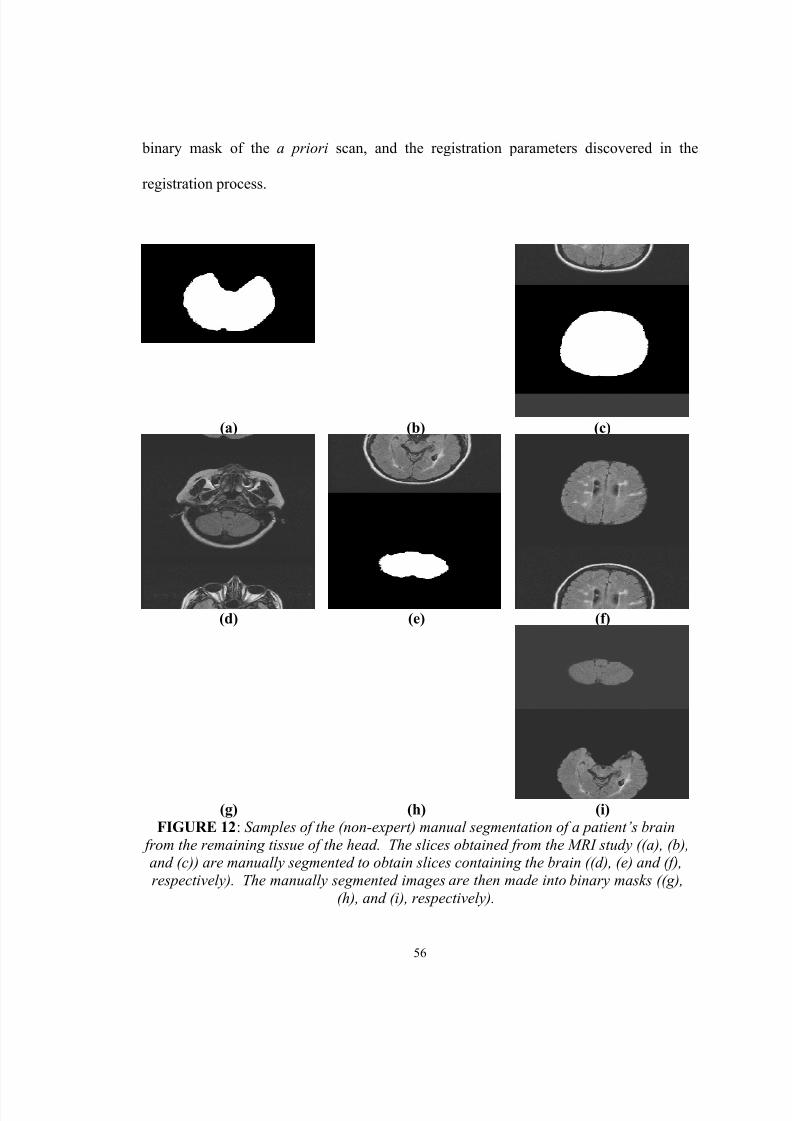
8/12/2019 Jeremy Nett
http://slidepdf.com/reader/full/jeremy-nett 71/124
56
binary mask of the a priori scan, and the registration parameters discovered in the
registration process.
(a) (b) (c)
(d) (e) (f)
(g) (h) (i)FIGURE 12 : Samples of the (non-expert) manual segmentation of a patient’s brain
from the remaining tissue of the head. The slices obtained from the MRI study ((a), (b),and (c)) are manually segmented to obtain slices containing the brain ((d), (e) and (f),respectively). The manually segmented images are then made into binary masks ((g),
(h), and (i), respectively).
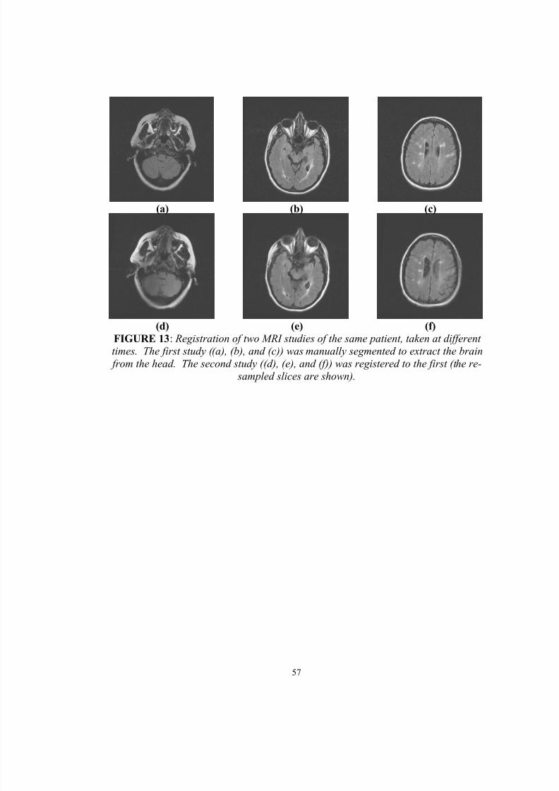
8/12/2019 Jeremy Nett
http://slidepdf.com/reader/full/jeremy-nett 72/124
57
(a) (b) (c)
(d) (e) (f)FIGURE 13 : Registration of two MRI studies of the same patient, taken at differenttimes. The first study ((a), (b), and (c)) was manually segmented to extract the brain from the head. The second study ((d), (e), and (f)) was registered to the first (the re-
sampled slices are shown).
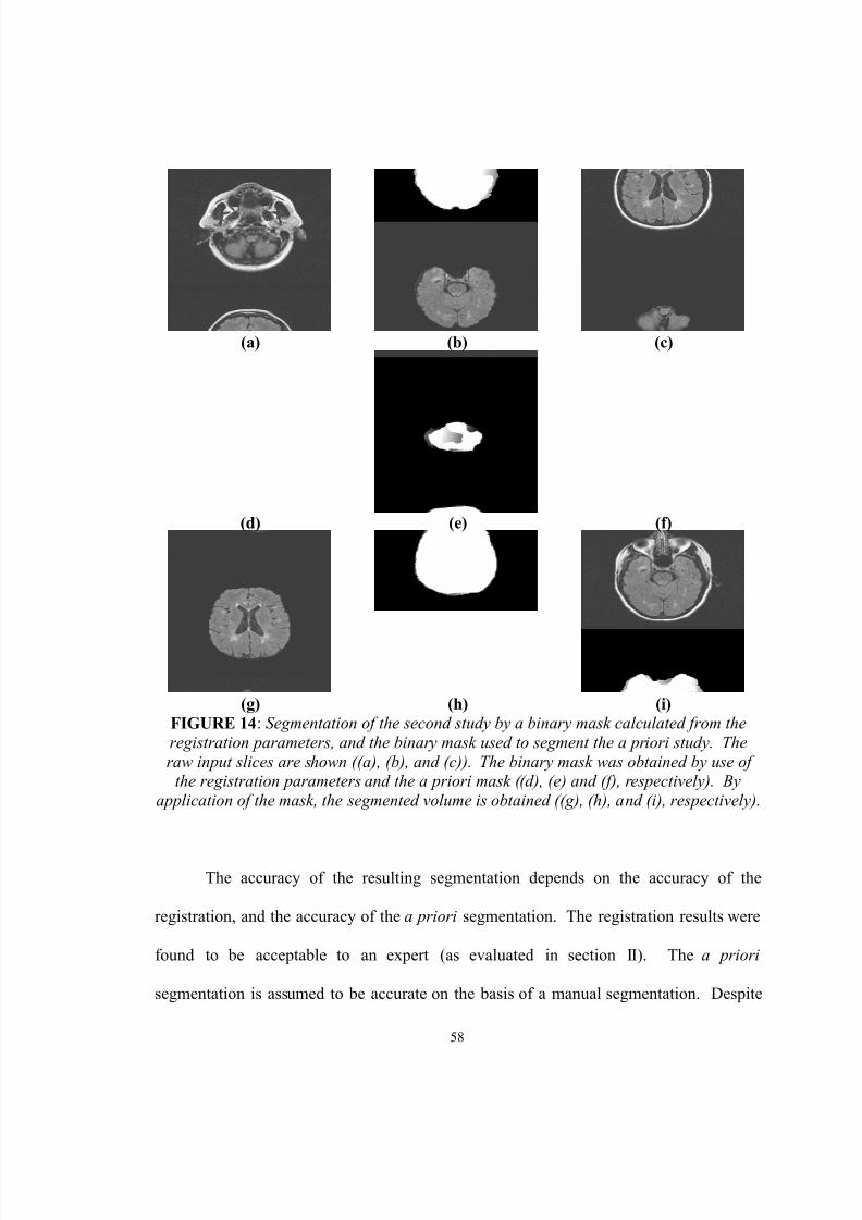
8/12/2019 Jeremy Nett
http://slidepdf.com/reader/full/jeremy-nett 73/124
58
(a) (b) (c)
(d) (e) (f)
(g) (h) (i)FIGURE 14 : Segmentation of the second study by a binary mask calculated from theregistration parameters, and the binary mask used to segment the a priori study. Theraw input slices are shown ((a), (b), and (c)). The binary mask was obtained by use of
the registration parameters and the a priori mask ((d), (e) and (f), respectively). Byapplication of the mask, the segmented volume is obtained ((g), (h), and (i), respectively).
The accuracy of the resulting segmentation depends on the accuracy of the
registration, and the accuracy of the a priori segmentation. The registration results were
found to be acceptable to an expert (as evaluated in section II). The a priori
segmentation is assumed to be accurate on the basis of a manual segmentation. Despite

8/12/2019 Jeremy Nett
http://slidepdf.com/reader/full/jeremy-nett 74/124
59
this argument, further work is necessary to numerically quantify the accuracy of the
segmentation.
D. Results: Semi-Automatic a priori Segmentation
Below are results obtained, when an initial a priori segmentation of a patient is
obtained by utilization of the segmentation tool, followed by manual re-labeling and
extraction of labels of interest. Figure 15 below shows sample results from the semi-
automatic segmentation method. The method is applied, and manual re-labeling is used
to identify the brain from the labels obtained in the segmentation. This re-labeling results
in a binary mask which can be used for extracting the brain from the head; the binary
mask obtained becomes the a priori brain mask. Figure 16 below shows sample results
from the registration of a second study to the a priori study, and application of the brain
mask obtained from the registration parameters and the a priori brain mask.
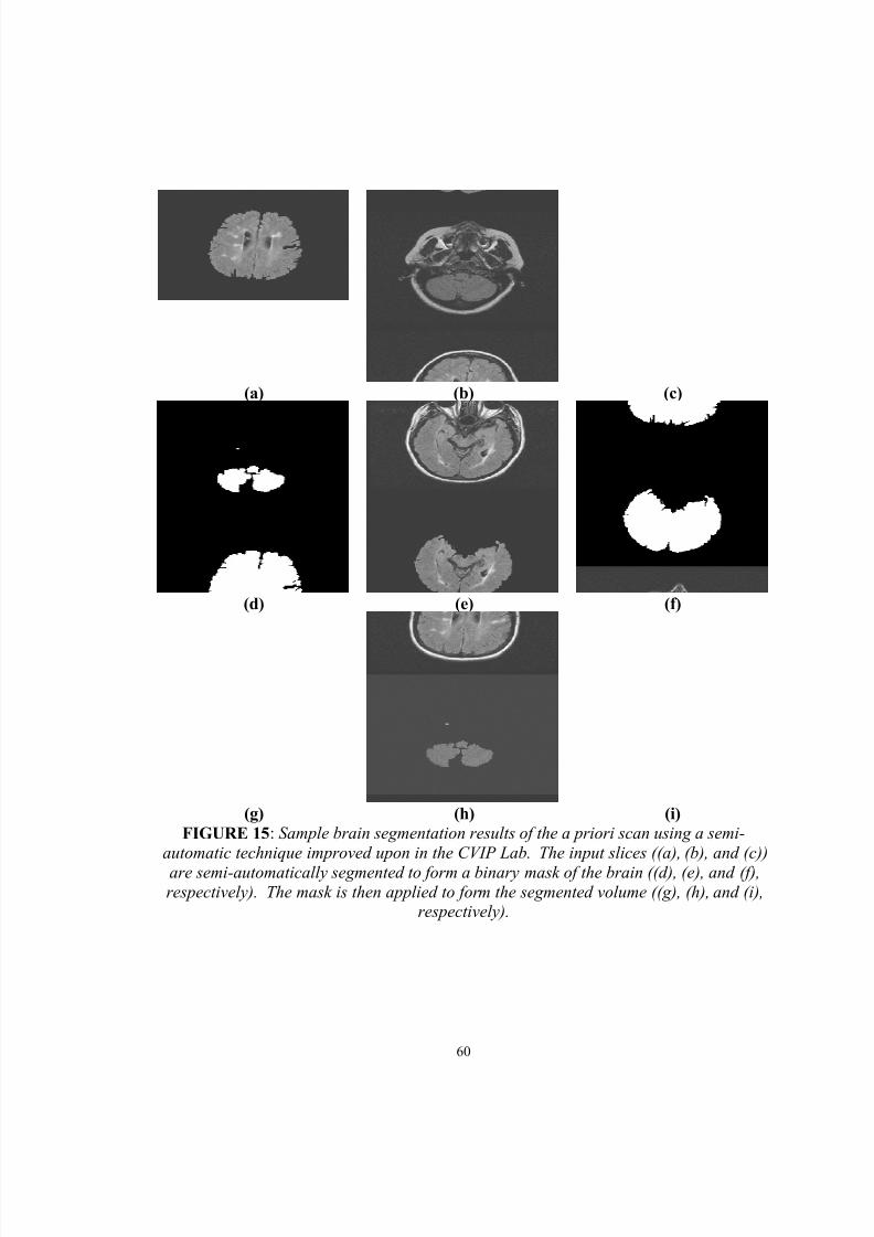
8/12/2019 Jeremy Nett
http://slidepdf.com/reader/full/jeremy-nett 75/124
60
(a) (b) (c)
(d) (e) (f)
(g) (h) (i)FIGURE 15 : Sample brain segmentation results of the a priori scan using a semi-
automatic technique improved upon in the CVIP Lab. The input slices ((a), (b), and (c))are semi-automatically segmented to form a binary mask of the brain ((d), (e), and (f),respectively). The mask is then applied to form the segmented volume ((g), (h), and (i),
respectively).

8/12/2019 Jeremy Nett
http://slidepdf.com/reader/full/jeremy-nett 76/124
61
(a) (b) (c)
(d) (e) (f)
(g) (h) (i)FIGURE 16 : Brain segmentation of the second study. The second study ((a), (b), and(c)) was registered to the a priori scan. The brain mask for the second study ((d), (e),
and (f), respectively) is then obtained using the a priori brain mask, and the registration parameters. The binary brain mask is then applied to generate the segmented volume
((g), (h), and (i), respectively).
As can be observed from the results of the semi-automatic method, there are
errors that prevent this approach from further use. For example, an MS lesion in the slice

8/12/2019 Jeremy Nett
http://slidepdf.com/reader/full/jeremy-nett 77/124
62
in figure 12 (c) is removed from the segmentation of the brain. Additionally, isolated
islands are present, as shown by the segmentation of the slice in figure 12 (a). Some
brain material is lost in the segmentation, as shown by the segmentation of the slice in
figure 12 (b).
E. Summary
Brain segmentation, the process of extracting the brain from the head, is a
necessary pre-processing step to classification of brain tissue in an MRI study of an MS
patient. To this end, segmentation via registration of a study to a study with a known
brain segmentation was explored, with useful results generated. The implemented
approach incurs a minimal amount of computational overhead, given that registration of
subsequent patient studies will be performed regardless of use in brain segmentation.
The manual procedure for generation of an a priori brain mask works well, but is
too demanding of human intervention to be useful in a clinical study of numerous
patients. The semi-automatic procedure, at present, does not generate accurate enough
brain segmentations to be used in a clinical study. Despite this, the segmentation may be
useful as an initial solution for manual segmentation.
8/12/2019 Jeremy Nett
http://slidepdf.com/reader/full/jeremy-nett 78/124
63
IV. TISSUE SEGMENTATION
A. Introduction and Necessity
Following segmentation of the brain from the remaining tissues imaged in the
head, tissue classification addresses the task of classifying tissues within this volume of
interest. States of nature, or classes, considered here include normal brain tissue (white
and gray matter), diseased or abnormal brain tissue (MS lesions), and CSF. From the
results of brain segmentation above, the operation of classification assigns a single class
to each voxel of this volume.
Resulting from this assignment of class, quantitative measures of MS disease
burden may be computed by computation of the total volume of MS lesions, and the total
volume of normal brain tissue. An increase in the volume of MS lesions is assumed to be
indicative of worsening of the disease. Decreases in the volume of normal brain material,
owing to brain atrophy and conversion of normal brain tissue to diseased tissue, are also
assumed to be indicative of worsening of the disease.
Several classification/segmentation schemes were experimented with over the
course of study of this problem, beginning with the very simple, and advancing to more
complicated, but necessary techniques to achieve good results.
A statistical classification approach, using the Bayes decision rule, is ultimately
utilized in the approach described here. Class conditional probabilities are estimated
nonparametrically, using Parzen windowing. A priori class probabilities are modeled
8/12/2019 Jeremy Nett
http://slidepdf.com/reader/full/jeremy-nett 79/124
64
using a Markov random field model. The results obtained demonstrate the effectiveness
of this approach.
B. Feature Selection
Generally obtained in the MS studies available for use, are T1, T2, and FLAIR
weighted MRI studies. The weighted studies are acquired simultaneously, and therefore,
no inter-study registration is necessary. Each weighting contrasts tissues with respect to
other tissues in the head differently. For example, with a T1 or FLAIR weighting, CSF is
“dark” relative to surrounding brain tissue, while in a T2 weighted study, CSF is “bright”
relative to surrounding brain tissue.
From a tissue classification perspective, different weightings provide for
additional raw features that may be useful in achieving improved classification. The
basis of this statement is that the use of additional features may help to provide
discriminatory power in feature space, such that there is reduced error in the resulting
classification by separation of feature measurements of tissues in the feature space. For
example, considering two tissue classes, and only one feature, there may be significant
overlap in feature space between the class conditional probability distributions of the
feature for the different classes. The inclusion of a second useful feature may allow for
improvement in the probability of error of the classifier, by allowing for improved
separation of tissues in feature space. With too many features, however, training
becomes difficult, the computation time of the classifier generally increases, and
performance of the classifier may actually decrease [33].
8/12/2019 Jeremy Nett
http://slidepdf.com/reader/full/jeremy-nett 80/124
65
Hyper-intense regions in the FLAIR studies are the desired regions to be
classified as MS lesions. In consideration of the additional weightings available (the T1
and T2 studies), it is observed that lesion appearance across the FLAIR, T1, and T2
studies is not consistent, as shown in figure 17. Comparing the appearance of the lesions
in the FLAIR image to T1 image, observing abnormal tissue in the T1 image is difficult
at best, and as a result, the T1 images are not useful for discrimination of lesions against
brain material. Comparing the appearance of the lesions in the FLAIR image to the T2
image, it is observed that the T2 image shows limited contrast of lesions against brain
material for some lesions. Furthermore, the diseased tissue imaged in the FLAIR image
is not always contrasted as abnormal tissue in the T2 image, and at other times, the
diseased material found in the T2 image appears quite differently depending on the
lesion.
Therefore, as the FLAIR image gives the best indications of disease, and because
the T1 and T2 images are either not useful (T1), or not consistent with the FLAIR
imagery (T2), the FLAIR imagery alone will be used for classification. The features that
will be used in classification will be the intensity observed in the FLAIR imagery.
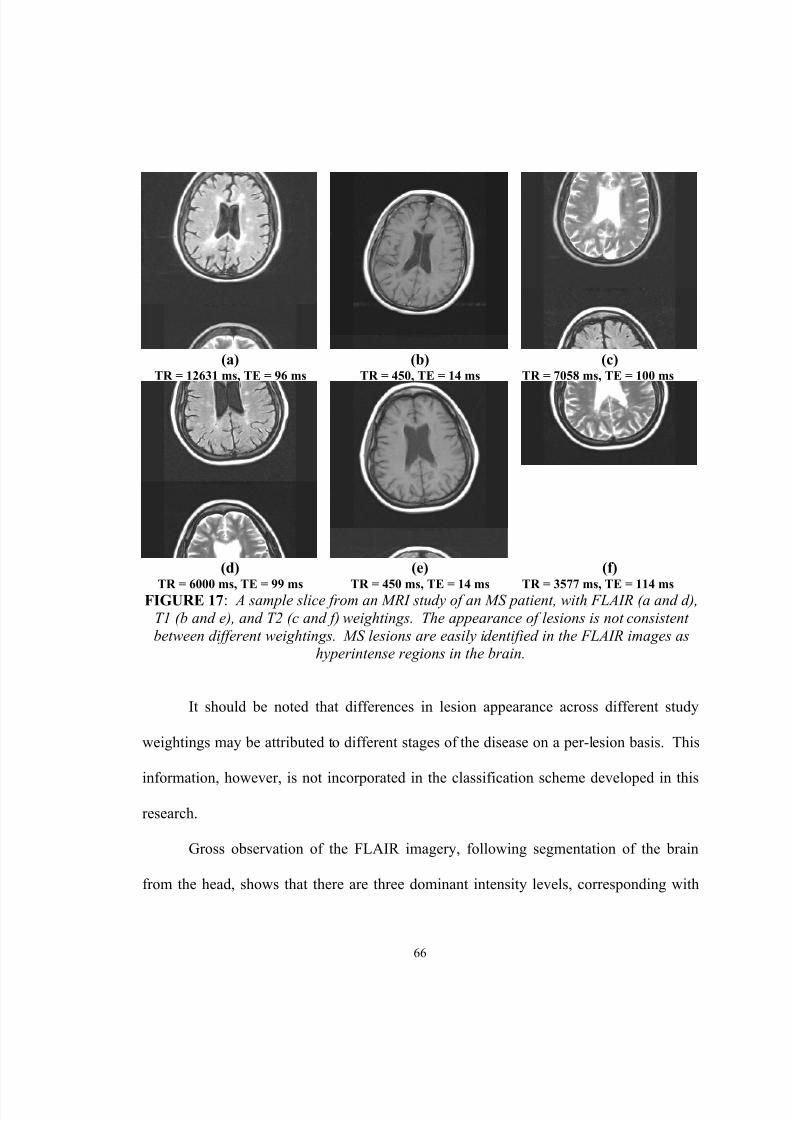
8/12/2019 Jeremy Nett
http://slidepdf.com/reader/full/jeremy-nett 81/124
66
(a)TR = 12631 ms, TE = 96 ms
(b)TR = 450, TE = 14 ms
(c)TR = 7058 ms, TE = 100 ms
(d)
TR = 6000 ms, TE = 99 ms
(e)
TR = 450 ms, TE = 14 ms
(f)
TR = 3577 ms, TE = 114 ms FIGURE 17 : A sample slice from an MRI study of an MS patient, with FLAIR (a and d),T1 (b and e), and T2 (c and f) weightings. The appearance of lesions is not consistentbetween different weightings. MS lesions are easily identified in the FLAIR images as
hyperintense regions in the brain.
It should be noted that differences in lesion appearance across different study
weightings may be attributed to different stages of the disease on a per-lesion basis. This
information, however, is not incorporated in the classification scheme developed in thisresearch.
Gross observation of the FLAIR imagery, following segmentation of the brain
from the head, shows that there are three dominant intensity levels, corresponding with
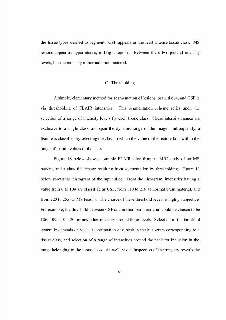
8/12/2019 Jeremy Nett
http://slidepdf.com/reader/full/jeremy-nett 82/124
67
the tissue types desired to segment. CSF appears as the least intense tissue class. MS
lesions appear as hyperintense, or bright regions. Between these two general intensity
levels, lies the intensity of normal brain material.
C. Thresholding
A simple, elementary method for segmentation of lesions, brain tissue, and CSF is
via thresholding of FLAIR intensities. This segmentation scheme relies upon the
selection of a range of intensity levels for each tissue class. These intensity ranges are
exclusive to a single class, and span the dynamic range of the image. Subsequently, a
feature is classified by selecting the class in which the value of the feature falls within the
range of feature values of the class.
Figure 18 below shows a sample FLAIR slice from an MRI study of an MS
patient, and a classified image resulting from segmentation by thresholding. Figure 19
below shows the histogram of the input slice. From the histogram, intensities having a
value from 0 to 109 are classified as CSF, from 110 to 219 as normal brain material, and
from 220 to 255, as MS lesions. The choice of these threshold levels is highly subjective.
For example, the threshold between CSF and normal brain material could be chosen to be
106, 109, 110, 120, or any other intensity around these levels. Selection of the threshold
generally depends on visual identification of a peak in the histogram corresponding to a
tissue class, and selection of a range of intensities around the peak for inclusion in the
range belonging to the tissue class. As well, visual inspection of the imagery reveals the
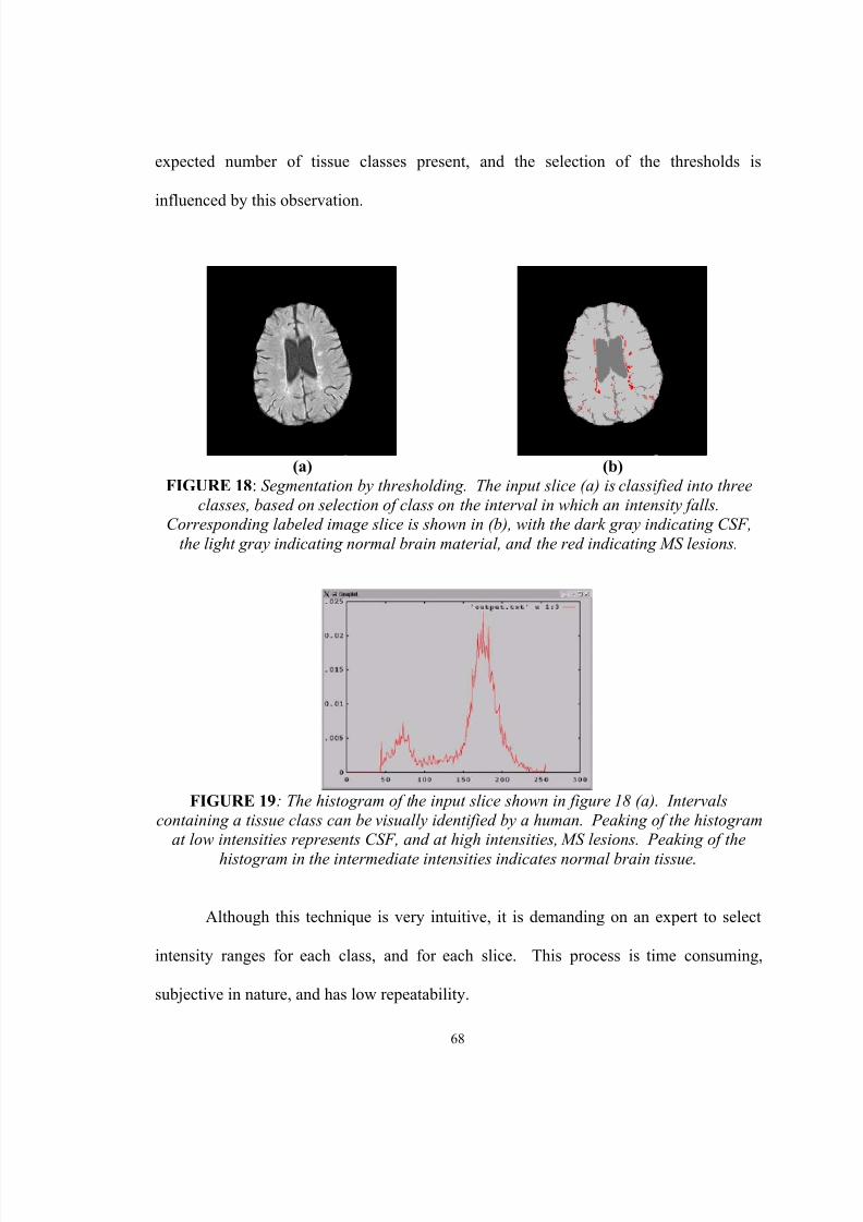
8/12/2019 Jeremy Nett
http://slidepdf.com/reader/full/jeremy-nett 83/124
68
expected number of tissue classes present, and the selection of the thresholds is
influenced by this observation.
(a) (b)FIGURE 18 : Segmentation by thresholding. The input slice (a) is classified into three
classes, based on selection of class on the interval in which an intensity falls.Corresponding labeled image slice is shown in (b), with the dark gray indicating CSF,
the light gray indicating normal brain material, and the red indicating MS lesions.
FIGURE 19 : The histogram of the input slice shown in figure 18 (a). Intervalscontaining a tissue class can be visually identified by a human. Peaking of the histogram
at low intensities represents CSF, and at high intensities, MS lesions. Peaking of thehistogram in the intermediate intensities indicates normal brain tissue .
Although this technique is very intuitive, it is demanding on an expert to select
intensity ranges for each class, and for each slice. This process is time consuming,
subjective in nature, and has low repeatability.
8/12/2019 Jeremy Nett
http://slidepdf.com/reader/full/jeremy-nett 84/124
69
D. Segmentation by Image Enhancement
A second image-processing approach to classification of the brain is segmentation
by image enhancement. In image processing terminology, an operation for image
enhancement improves the quality of the image in a particular manner, either
subjectively, or objectively. In the context of segmentation, an MRI slice of the brain
may be viewed as an image upon which enhancement may be performed. This model
assumes that a tissue class ideally has a single intensity, and that noise and scanning
artifacts corrupt this level to produce the distribution of intensities observed for a tissue
class. Thus, by application of image enhancement techniques for reducing noise and
smoothing the image, the enhanced image approximates the ideal image, at least to a
greater extent than the original image.
A class of filters known as nonlinear anisotropic diffusion filters can be useful for
image enhancement [32], as discussed for pre-filtering MRI data before the application of
the head labeling technique previously. As aforementioned, this class of filters performs
smoothing while preserving edges. The smoothing procedure is modeled as a local
diffusion process. For 2D isotropic image filtering, the fundamental equation for an
iteration of the filter is given below in eq. 26, where I(x,y,t) is the intensity of the image
at coordinates (x,y), at a time t, and c(i) is known as a diffusion function [32].
8/12/2019 Jeremy Nett
http://slidepdf.com/reader/full/jeremy-nett 85/124
70
[ ]
),1,(),,(
),,(),1,(),,1(),,(
),,(),,1(
)()()()(),,(),,(
t y x I t y x I s
t y x I t y x I nt y x I t y x I w
t y x I t y x I e
sc sncnwcwecet t y x I t t y x I
−−=−+=
−−=
−+=⋅−⋅+⋅−⋅⋅∆+≈∆+
(26)
Eq. 26 incorporates numerical integration to obtain a final enhanced image I. The
time t orders the sequence of progressively enhanced images. The quantity ∆t controls
the time step size, and affects the accuracy of the integration, and hence, the stability of
the filter. A value of 0.2 for the time step was simply selected, and in no cases, resulted
in observed instability of the filter when used with the experiments presented here. An
exponential function is used here for c(i), and is given below in eq. 27, where κ is a
constant known as the diffusion constant [32].
−=
2||
exp)(κi
ic (27)
The diffusion constant κ controls the effect of the filter. The value of 8.0 was
used in the studies here for image enhancement. This value was chosen experimentally,
to give the best results visually for a study. It was observed that a constant value of this
parameter produced consistent results across different studies.
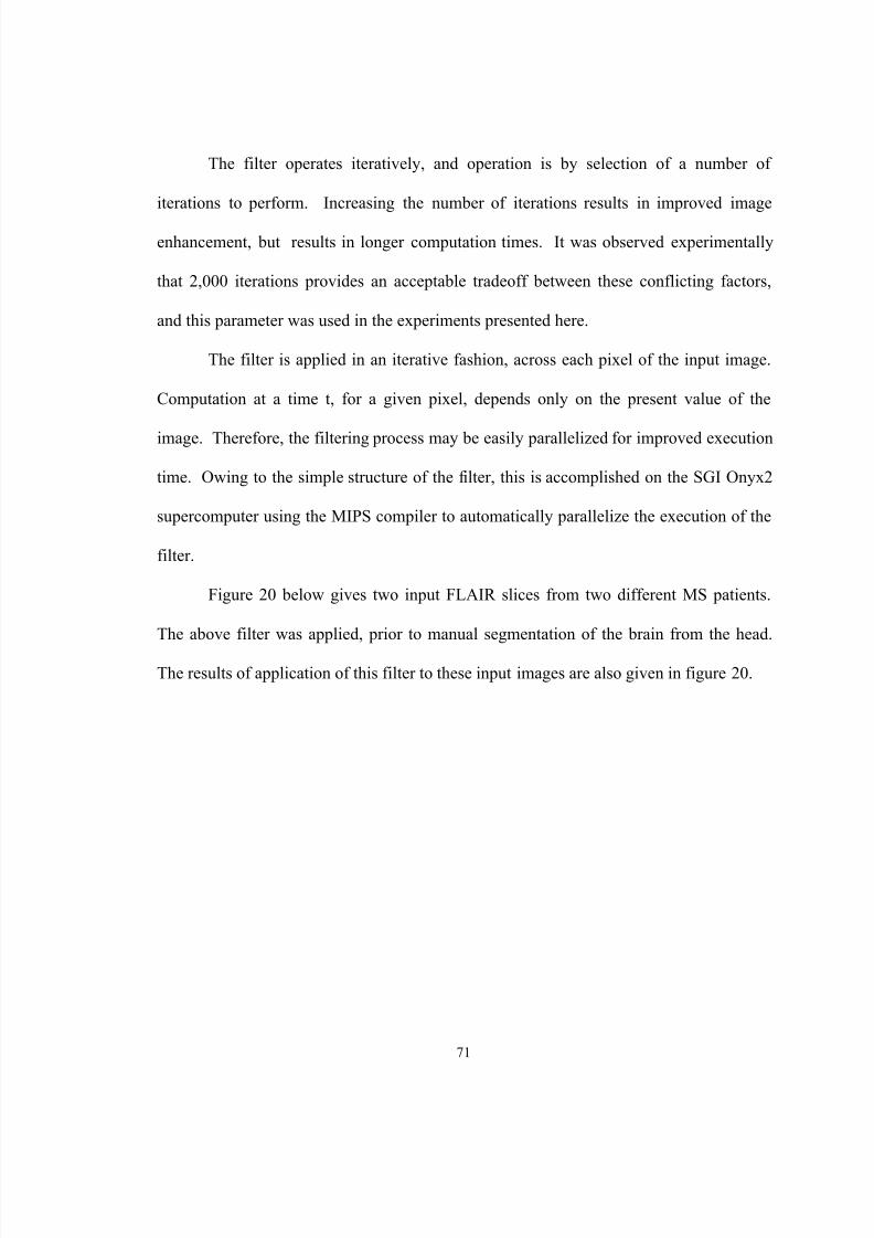
8/12/2019 Jeremy Nett
http://slidepdf.com/reader/full/jeremy-nett 86/124
71
The filter operates iteratively, and operation is by selection of a number of
iterations to perform. Increasing the number of iterations results in improved image
enhancement, but results in longer computation times. It was observed experimentally
that 2,000 iterations provides an acceptable tradeoff between these conflicting factors,
and this parameter was used in the experiments presented here.
The filter is applied in an iterative fashion, across each pixel of the input image.
Computation at a time t, for a given pixel, depends only on the present value of the
image. Therefore, the filtering process may be easily parallelized for improved execution
time. Owing to the simple structure of the filter, this is accomplished on the SGI Onyx2
supercomputer using the MIPS compiler to automatically parallelize the execution of the
filter.
Figure 20 below gives two input FLAIR slices from two different MS patients.
The above filter was applied, prior to manual segmentation of the brain from the head.
The results of application of this filter to these input images are also given in figure 20.
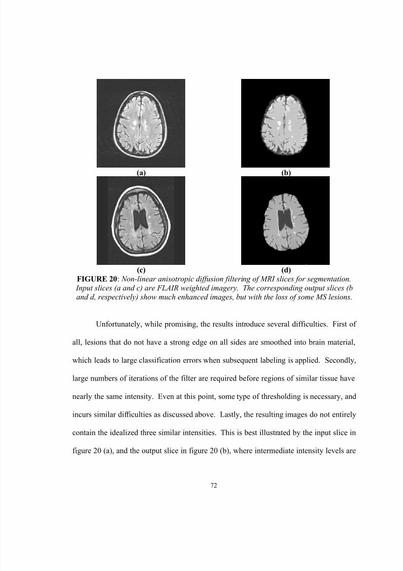
8/12/2019 Jeremy Nett
http://slidepdf.com/reader/full/jeremy-nett 87/124
72
(a) (b)
(c) (d)FIGURE 20 : Non-linear anisotropic diffusion filtering of MRI slices for segmentation.
Input slices (a and c) are FLAIR weighted imagery. The corresponding output slices (b
and d, respectively) show much enhanced images, but with the loss of some MS lesions.
Unfortunately, while promising, the results introduce several difficulties. First of
all, lesions that do not have a strong edge on all sides are smoothed into brain material,
which leads to large classification errors when subsequent labeling is applied. Secondly,
large numbers of iterations of the filter are required before regions of similar tissue have
nearly the same intensity. Even at this point, some type of thresholding is necessary, andincurs similar difficulties as discussed above. Lastly, the resulting images do not entirely
contain the idealized three similar intensities. This is best illustrated by the input slice in
figure 20 (a), and the output slice in figure 20 (b), where intermediate intensity levels are
8/12/2019 Jeremy Nett
http://slidepdf.com/reader/full/jeremy-nett 88/124
73
obtained, corresponding to blurred regions and scanning artifacts in the input slice.
Figure 21 below illustrates some of the types of errors encountered.
FIGURE 21 : Illustration of types of errors encountered with segmentation via imageenhancement.
E. Segmentation by Unsupervised Clustering
Clustering methods are algorithms that operate on an input data set, grouping data
into clusters based on similarity of the data in like clusters. As such, clustering
algorithms are unsupervised classifiers, assigning states of nature without regard to any a
priori labeled training samples. Clustering algorithms are also useful for data
exploration, allowing a user to discover patterns or similarities in a data set [33].

8/12/2019 Jeremy Nett
http://slidepdf.com/reader/full/jeremy-nett 89/124
74
Explored in this research are clustering techniques for unsupervised classification.
A well-known clustering algorithm, k-means clustering, was implemented, and tested on
sample slices of FLAIR weighted MRI slices from MS patients.
The k-means algorithm accepts as input the number of clusters to organize data
within, initial location of cluster centers, and a data set to cluster.
The number of clusters that the algorithm fits the data to, denoted by c, is
specified to the algorithm, and represents a parameter the user desires to experiment with,
or as a parameter expressing the expected or desired number of classes to discern from
the data. With the k-means algorithm proper, there are no conditions upon which c is
decreased or increased. Additionally, there are no conditions upon which data is
excluded or included in consideration of fit to classes; all data provided as input to the
algorithm is classified. A given piece of data, or feature measurement, is assigned
exclusively to one class (as compared to fuzzy k-means clustering, where a degree of
membership is assigned to each data item, for each class).
Initial cluster centers are provided here as random locations in feature space.
There is a cluster center µ i for each cluster, such that i = 1… c. Each cluster center is a d -
component column vector, where d is the number of input features in the data set. For
the case of a single feature taken to be the intensity of the FLAIR study, d = 1.
The data set provided to the k-means algorithm consists of N items, with each
item a d -component column vector, denoted as xi, i = 1…N.
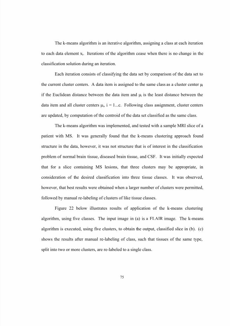
8/12/2019 Jeremy Nett
http://slidepdf.com/reader/full/jeremy-nett 90/124
75
The k-means algorithm is an iterative algorithm, assigning a class at each iteration
to each data element x i. Iterations of the algorithm cease when there is no change in the
classification solution during an iteration.
Each iteration consists of classifying the data set by comparison of the data set to
the current cluster centers. A data item is assigned to the same class as a cluster center µ i
if the Euclidean distance between the data item and µ i is the least distance between the
data item and all cluster centers µ i, i = 1...c. Following class assignment, cluster centers
are updated, by computation of the centroid of the data set classified as the same class.
The k-means algorithm was implemented, and tested with a sample MRI slice of a
patient with MS. It was generally found that the k-means clustering approach found
structure in the data, however, it was not structure that is of interest in the classification
problem of normal brain tissue, diseased brain tissue, and CSF. It was initially expected
that for a slice containing MS lesions, that three clusters may be appropriate, in
consideration of the desired classification into three tissue classes. It was observed,
however, that best results were obtained when a larger number of clusters were permitted,
followed by manual re-labeling of clusters of like tissue classes.
Figure 22 below illustrates results of application of the k-means clustering
algorithm, using five classes. The input image in (a) is a FLAIR image. The k-means
algorithm is executed, using five clusters, to obtain the output, classified slice in (b). (c)
shows the results after manual re-labeling of class, such that tissues of the same type,
split into two or more clusters, are re-labeled to a single class.
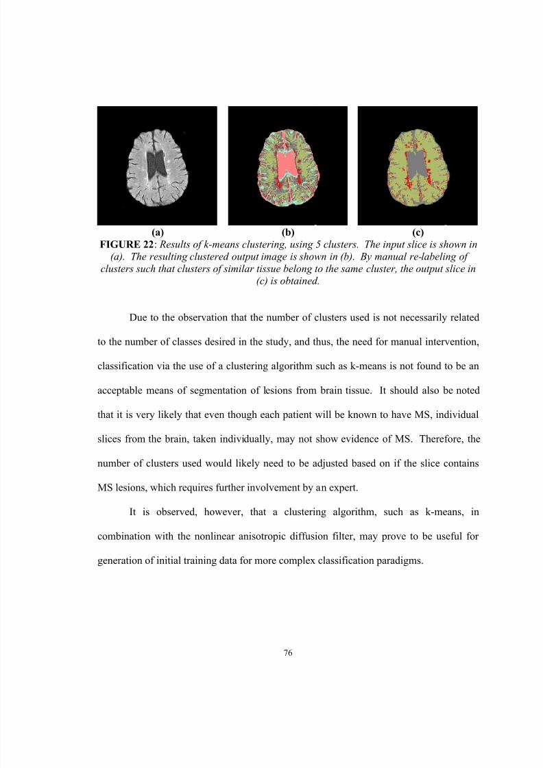
8/12/2019 Jeremy Nett
http://slidepdf.com/reader/full/jeremy-nett 91/124
76
(a) (b) (c)FIGURE 22 : Results of k-means clustering, using 5 clusters. The input slice is shown in
(a). The resulting clustered output image is shown in (b). By manual re-labeling of
clusters such that clusters of similar tissue belong to the same cluster, the output slice in(c) is obtained.
Due to the observation that the number of clusters used is not necessarily related
to the number of classes desired in the study, and thus, the need for manual intervention,
classification via the use of a clustering algorithm such as k-means is not found to be an
acceptable means of segmentation of lesions from brain tissue. It should also be noted
that it is very likely that even though each patient will be known to have MS, individual
slices from the brain, taken individually, may not show evidence of MS. Therefore, the
number of clusters used would likely need to be adjusted based on if the slice contains
MS lesions, which requires further involvement by an expert.
It is observed, however, that a clustering algorithm, such as k-means, in
combination with the nonlinear anisotropic diffusion filter, may prove to be useful for
generation of initial training data for more complex classification paradigms.
8/12/2019 Jeremy Nett
http://slidepdf.com/reader/full/jeremy-nett 92/124
77
F. Bayesian Classification
The above approaches, while generating tantalizing results, all fail with regard to
accuracy, ease of application, and logical relation to the classification problem. A
statistical classification approach addressees these concerns, providing an optimal
solution to the classification problem when tissue models are known or well
approximated. Additionally, statistical classification is well founded in probability
theory, and has enjoyed success in a number of applications, including classification of
remote sensing data, scene classification, and classification of medical imagery.
Statistical classification is fundamentally based upon the application of Bayes rule
for quantifying a decision procedure. Bayes rule, given in eq. 28 below, specifies how to
compute a posterior probability of a class, given feature measurements [33].
)(
)()|()|(
x p
P x p x P j j
j
ωωω
⋅=
(28)
In eq. 28, ω j denotes a class, or state of nature. The vector x denotes a feature
vector, obtained from measurements of quantities of interest. For image analysis, thefeature vector x is composed for each pixel, and consists of the features of the pixel. For
the approach here, the feature x therefore shall consist of one component, the intensity of
the pixel from the FLAIR image. The quantity p(x| ω j) is known as the class conditional

8/12/2019 Jeremy Nett
http://slidepdf.com/reader/full/jeremy-nett 93/124
78
probability density function for class ω j. This distribution quantifies the probability of
measurement of a feature, given a state of nature. The quantity P( ω j) is known as the a
priori probability, and quantifies the probability of observing a state of nature, regardless
of any feature measurement. The quantity p(x) is known as the evidence, and serves only
as a scale factor, such that the quantity in eq. 28 is indeed a true probability, with values
between zero and one. The quantity P( ω j|x) is known as the posterior probability, and
quantifies the probability of observing class ω j, given that the feature x was measured.
The quantity p(x) in eq. 28 can normally be ignored for implementing decision
theory, as it is only a constant for establishing a probability between zero and one, and
constant for all classes. Therefore, the quantity given below in eq. 29, known as the
maximum a posteriori (MAP) estimate of eq. 28, is used.
)()|()|( j j j P x p x P ωωω ⋅= (29)
Bayes decision rule, based upon the application of eq. 28 or 29, gives a
framework for how to make a sound decision. For c possible classes, Bayes decision rule
mandates the selection of class ω j for a feature x , if the a posteriori quantities in eq. 28 or29 are maximum for class ω j, compared to ω i, i = 1…c, i ≠ j. This rule is stated below in
eq. 30 [33].
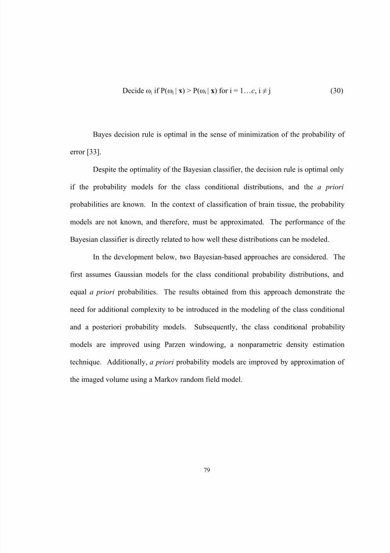
8/12/2019 Jeremy Nett
http://slidepdf.com/reader/full/jeremy-nett 94/124
79
Decide ω j if P( ω j | x) > P( ω i | x) for i = 1… c, i ≠ j (30)
Bayes decision rule is optimal in the sense of minimization of the probability of
error [33].
Despite the optimality of the Bayesian classifier, the decision rule is optimal only
if the probability models for the class conditional distributions, and the a priori
probabilities are known. In the context of classification of brain tissue, the probability
models are not known, and therefore, must be approximated. The performance of the
Bayesian classifier is directly related to how well these distributions can be modeled.
In the development below, two Bayesian-based approaches are considered. The
first assumes Gaussian models for the class conditional probability distributions, and
equal a priori probabilities. The results obtained from this approach demonstrate the
need for additional complexity to be introduced in the modeling of the class conditional
and a posteriori probability models. Subsequently, the class conditional probability
models are improved using Parzen windowing, a nonparametric density estimation
technique. Additionally, a priori probability models are improved by approximation of
the imaged volume using a Markov random field model.

8/12/2019 Jeremy Nett
http://slidepdf.com/reader/full/jeremy-nett 95/124
80
G. Bayesian Classification: Gaussian Conditionals, Equal a priori Probabilities
As an initial approach, class conditional probabilities are modeled using a
Gaussian distribution, and in the absence of any other information, equal a posteriori
probabilities are assumed [34].
The general form of a Gaussian probability distribution is given below in eq. 31.
In the context of the present problem, a single feature is used, being the intensity from the
FLAIR imagery. The form of a univariate distribution is given below in eq. 32.
In eq. 31, d is the dimension of the distribution, Σ represents the d x d covariance
matrix, x is a d -component column vector, and µ is a d -component mean vector. In eq.
32, σ is the standard deviation, x is a scalar, and µ is the mean value of the distribution.
−Σ−−
Σ= − )()(
21exp
)2(
1)|( 1
21
2µµ
πω x x x p t
d j (31)
−−=
2
21
exp2
1)|(
σµ
σπω x
x p j (32)
As no information is known otherwise, the a posteriori probabilities for each class
are assumed to be equal. Therefore, for three classes, the probability P( ω i) is equal to 1/3
for each class. These probabilities are equal for each class, and therefore, do not affect
the result of the computation of eq. 28 or 29, and therefore, for the case considered here,
8/12/2019 Jeremy Nett
http://slidepdf.com/reader/full/jeremy-nett 96/124
81
the posterior quantity upon which a decision is made is given completely by the result of
the computation of eq. 32.
From manually selected training samples, the mean µ and the standard deviation σ
are estimated using the maximum likelihood estimators (MLEs) for a univariate Gaussian
probability distribution function, given below in eqs. 33 and 34, respectively [35]. The
MLE estimates of the mean and standard deviation are µ’ and σ’, respectively. The
quantity n represents the number of training samples available, and x k is the k th training
sample.
∑=
=n
k k x
n 1
' 1µ (33)
( ) ∑=
−=n
k k x
n 1
2''2 )(1 µσ
(34)
Below in figure 23, a sample result of the application of this scheme is presented.
In terms of performance, this classifier performs poorly. Upon close evaluation,
however, it is evident that the classifier works decently when the tissue is completely
unambiguous, and not in close proximity to boundaries with other tissues. For example,
the classification of normal brain material works well when not in close proximity to MS
lesions, and vice-versa. Based on the sample slice presented below in figure 23, as well
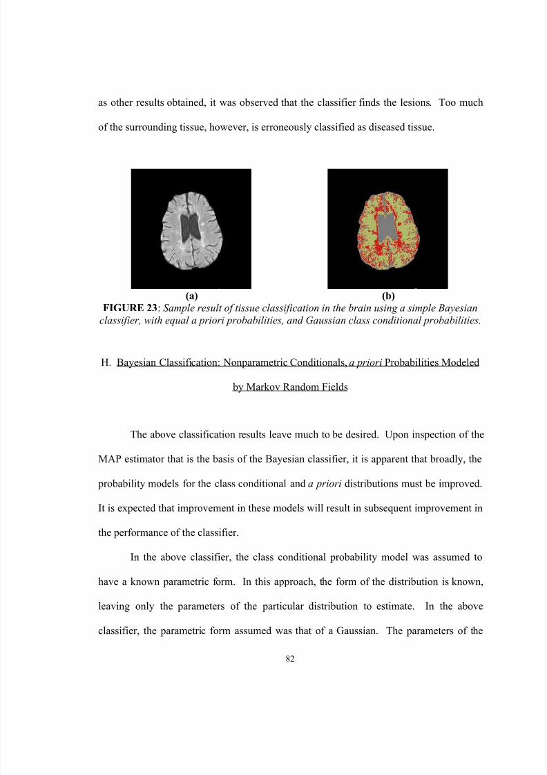
8/12/2019 Jeremy Nett
http://slidepdf.com/reader/full/jeremy-nett 97/124
82
as other results obtained, it was observed that the classifier finds the lesions. Too much
of the surrounding tissue, however, is erroneously classified as diseased tissue.
(a) (b)FIGURE 23 : Sample result of tissue classification in the brain using a simple Bayesian
classifier, with equal a priori probabilities, and Gaussian class conditional probabilities.
H. Bayesian Classification: Nonparametric Conditionals, a priori Probabilities Modeled
by Markov Random Fields
The above classification results leave much to be desired. Upon inspection of the
MAP estimator that is the basis of the Bayesian classifier, it is apparent that broadly, the
probability models for the class conditional and a priori distributions must be improved.
It is expected that improvement in these models will result in subsequent improvement in
the performance of the classifier.
In the above classifier, the class conditional probability model was assumed to
have a known parametric form. In this approach, the form of the distribution is known,
leaving only the parameters of the particular distribution to estimate. In the above
classifier, the parametric form assumed was that of a Gaussian. The parameters of the

8/12/2019 Jeremy Nett
http://slidepdf.com/reader/full/jeremy-nett 98/124
83
Gaussian distribution, the mean and the standard deviation, were estimated using
maximum likelihood estimators.
A more general approach involves the use of nonparametric techniques for
density estimation [33]. Such approaches allow for direct estimation of the probability
distribution, eliminating the necessity of choosing a parametric form of the class
conditional distribution. Assumption of a parametric form is acceptable, if it is known
that the true distribution is Gaussian, or if a Gaussian is a good approximation to the true
class conditional distribution.
Use of a nonparametric technique, however, removes the need for the assumption
and estimation of the parameters of the assumed parametric model. Instead, the
probability distribution is estimated directly from the training data.
The nonparametric technique known as Parzen windowing is used here to
improve the model of the class conditional probabilities [33]. For each tissue class,
training samples are used to form an estimated probability distribution. The estimated
probability distribution is given by evaluation of eq. 35 below, where n is the number of
training samples, and δ(x) is a Parzen window function, taken to be a Gaussian kernel,
with a mean of zero, and a variance of one, here.
( )∑=
−=n
ii j x x
n x p
1
1)|( δω
(35)

8/12/2019 Jeremy Nett
http://slidepdf.com/reader/full/jeremy-nett 99/124
84
Estimation using the Parzen window estimate of eq. 35 can be made
computationally efficient by the generation of look-up tables for p(x| ω j). The use of
look-up tables avoids the computation of a sum, of a large number of training samples ( n
of them), at each evaluation for some x and ω j.
The a priori probabilities P( ω j) were assumed in the simple Bayesian classifier,
above, to be equal for each tissue class. This assumption, however, is not well justified.
For example, in the input slice in figure 21 (a), it is very apparent that the probability of
normal brain material exceeds that of abnormal brain material. In the improvement of the
simple Bayesian classifier, then, it is also necessary to consider a more appropriate model
for the a priori probabilities.
It is reasonable to consider an a priori probability on a local scale, and consider
the spatial nature of the feature measurements obtained from MRI studies of the brain. A
feature measurement has a spatial location within the brain. If this feature measurement
is known to have a state of nature of ω i, then it is reasonable to assume that the feature
measurements surrounding this known voxel have an increased probability of also having
a state of nature of ω i. This assumption is reasonable, as there is order to anatomy
imaged, with abnormal brain material forming in regions, for example. The opposite of
this observation would be to take a slice, such as shown in figure 21 (a), and randomly
swap voxels until there is no region homogeneity in the image.
Markov random field (MRF) models [36, 37] provide such a modeling of
neighborhood influences that can be utilized to form an improved probability model for
the a priori probability P( ω j).

8/12/2019 Jeremy Nett
http://slidepdf.com/reader/full/jeremy-nett 100/124
85
A Markov random field models an image or volume as a random field, a
structured collection of random variables, F = {F 1, …, F m}, and defined on the set S.
Here, each random variable is a lattice point in the sampled volume. A Markov random
field is a special case of a random field. There are two conditions imposed to allow a
random field to be labeled as a Markov random field [36]:
1. F f f p ∈∀> ,0)( , known as the positivity condition
2. )|()|( }{ i N iiS i f f p f f p =− , known as the Markovianity condition
The positivity condition is implicitly satisfied with the application of the Markov
random field model of a priori probabilities. The Markovianity condition states that the
probability of an observation f i, given the other random variables in the field, is equal to
the probability of the observation f i, given a neighborhood around the sampled location,
denoted as N i. This statement fits well with the above reasoning, with respect to
consideration of local areas around a voxel to assist in formulating the a priori class
probability P( ω i).
Neighborhood structures are regions surrounding a sample, and chosen for
incorporation into the a priori probability model. For a regular sampling lattice (such as
the images here), a neighborhood is characterized by its order r , with the order defining
the nature of the neighborhood. The order r is related to the neighboring samples that are
included in the probability model by considering a circle of radius r . Figure 24 below
illustrates neighborhood structures for an image.
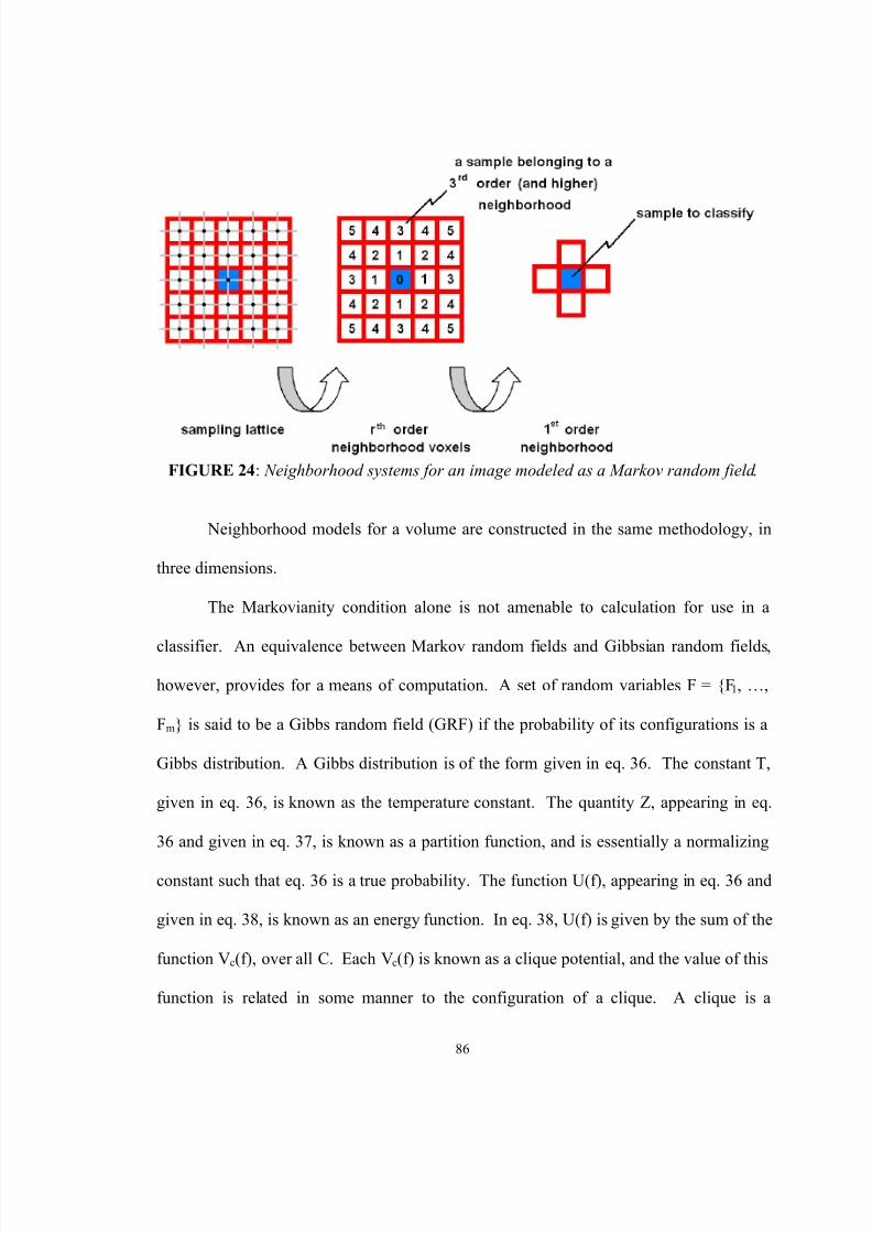
8/12/2019 Jeremy Nett
http://slidepdf.com/reader/full/jeremy-nett 101/124
86
FIGURE 24 : Neighborhood systems for an image modeled as a Markov random field .
Neighborhood models for a volume are constructed in the same methodology, in
three dimensions.
The Markovianity condition alone is not amenable to calculation for use in a
classifier. An equivalence between Markov random fields and Gibbsian random fields,
however, provides for a means of computation. A set of random variables F = {F 1, …,
Fm} is said to be a Gibbs random field (GRF) if the probability of its configurations is a
Gibbs distribution. A Gibbs distribution is of the form given in eq. 36. The constant T,
given in eq. 36, is known as the temperature constant. The quantity Z, appearing in eq.
36 and given in eq. 37, is known as a partition function, and is essentially a normalizing
constant such that eq. 36 is a true probability. The function U(f), appearing in eq. 36 and
given in eq. 38, is known as an energy function. In eq. 38, U(f) is given by the sum of the
function V c(f), over all C. Each V c(f) is known as a clique potential, and the value of this
function is related in some manner to the configuration of a clique. A clique is a
8/12/2019 Jeremy Nett
http://slidepdf.com/reader/full/jeremy-nett 102/124
87
grouping of samples in a neighborhood system, such that the grouping includes voxels
that are neighbors of one another in the same system.
−= )(
1exp
1)( f U
T Z f p
(36)
∑
−=
F
f U T
Z )(1
exp(37)
∑=C
c f V f U )()( (38)
A result known as the Hammersley-Clifford theorem states that if and only if a
random field F on S is a Markov random field with respect to a neighborhood system N ,
then F is a Gibbs random field on S with respect to a neighborhood system N [36]. This
result allows the conditional probability given as the Markovianity condition of an MRF
to be converted to the non-conditional probability of a Gibbs distribution, given in eq. 36.
This allows for computation of the a priori class probabilities modeled as an MRF, and
therefore, incorporation of this model into a practical classifier.
In the classifier constructed here, a simple model for the energy function U(f) is
utilized [38]. This model consists of a linear combination of products of elements in the
cliques. For experimentation, a first order neighborhood system for image segmentation
is considered. The resulting model for U(f) is given below in eq. 39.

8/12/2019 Jeremy Nett
http://slidepdf.com/reader/full/jeremy-nett 103/124
88
( ) ( )( )1,1,2,1,11,, )()( +−+− +⋅++⋅+⋅== l k l k l k l k l k l k f f f f f f U f U ββα (39)
The quantity f i,j in eq. 39 refers to the sample at indices (i,j) in the labeled image.
The parameters α, β1, and β2 are parameters that allow for adjusting relative weights or
contributions of neighborhood interactions. In the experiments here, α is taken to be 1.0,
and β1 and β2 are both taken to be 0.75. These weightings allow the current classificationat index (i, j) to take an importance somewhat greater than the neighborhood
classifications, and gives equal weighting to the neighbors of the feature measured at (i,
j). Also, it should be noted that the temperature parameter T is taken to be 1.0.
The implemented algorithm accepts a slice of data, and training points. An initial
classification solution is obtained by assumption of equal a priori class probabilities.
Subsequent iterations implement modeling of a priori class probabilities using the MRF
model discussed above. Each iteration classifies the entire image, using the previous
classification as a basis to model neighborhood interactions. The iterative process
terminates when no changes are made in the classification. Class conditional
probabilities are modeled throughout from the training points initially supplied.
A sample of the results obtained is given below in figure 25. The classifier
successfully detects the lesions, and in general, is observed to perform well. Additional
comments on the behavior of the classifier are given below. In terms of computational
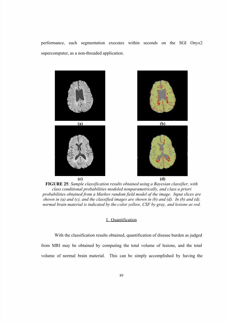
8/12/2019 Jeremy Nett
http://slidepdf.com/reader/full/jeremy-nett 104/124
89
performance, each segmentation executes within seconds on the SGI Onyx2
supercomputer, as a non-threaded application.
(a) (b)
(c) (d)FIGURE 25 : Sample classification results obtained using a Bayesian classifier, with
class conditional probabilities modeled nonparametrically, and class a priori probabilities obtained from a Markov random field model of the image. Input slices are shown in (a) and (c), and the classified images are shown in (b) and (d). In (b) and (d),normal brain material is indicated by the color yellow, CSF by gray, and lesions as red.
I. Quantification
With the classification results obtained, quantification of disease burden as judged
from MRI may be obtained by computing the total volume of lesions, and the total
volume of normal brain material. This can be simply accomplished by having the

8/12/2019 Jeremy Nett
http://slidepdf.com/reader/full/jeremy-nett 105/124
90
computer count the number of labels assigned for each class, and then multiplying this
number by the volume of each voxel, which is known a priori from the scanner. Results
of this process are given in Table IV, below, for the output slices given in figure 25.
TABLE IVQUANTIFICATION OF MS DISEASE BURDEN FROM THE SAMPLE RESULTS
GIVEN IN FIGURE 25.
InputSlice
Number
ofnormalbraintissuevoxels
Number
ofabnormalbraintissuevoxels
Volumeof normal
braintissue(mm 3)
Volume
ofabnormalbraintissue(mm 3)
Percentage
of normalbrain tissuevolume tototal brain
volume
Percentageof
abnormalbrain tissuevolume tototal brain
volumeFigure.23 (a) 12222 1,463 53709.960 6429.199 89.3 % 10.7 %
Figure23 (c) 13920 1,053 61171.875 4627.441 93.0 % 7.0 %
J. Accuracy
The results obtained subjectively show good performance. Lesions are detected,
and highlighted. The classifier erroneously detects lesions around the outer perimeter of
the brain, mistaking scanning artifacts with MS lesions.
Results were shown to Dr. Robert Falk, a radiologist at Jewish Hospital. Dr.
Falk’s comments on the results obtained were positive.
8/12/2019 Jeremy Nett
http://slidepdf.com/reader/full/jeremy-nett 106/124
91
K. Summary
Pattern recognition approaches were explored for classification of the tissues
present in the brain. Several approaches were attempted, including image processing
approaches using thresholding and image enhancement, unsupervised classification via
the use of the k-means algorithm, and statistical classification utilizing Bayes rule, with
Gaussian probability models for class conditional probability distributions.
Improvement of the statistical classifier by nonparametric modeling of the class
conditional probability distributions using Parzen windowing, and modeling of the a
priori class probabilities via the use of a Markov random field image model, provided the
best results obtained. Quantification of MS may then be implemented by computing the
total volume of normal and diseased brain material, from the resulting states of nature
assigned by the classifier and the voxel sizes used in the acquisition of the study.
8/12/2019 Jeremy Nett
http://slidepdf.com/reader/full/jeremy-nett 107/124
92
V. VISUALIZATION
A. Introduction
Several scientific visualization techniques are applied here for the study of the
results of the registration and segmentation processes implemented. For the evaluation of
the volume registration results, a simple data fusion technique is applied, which overlaps
regions of the floating and re-sampled reference volumes. As well, a visualization
application is presented which allows for volume rendering, and re-slicing volumes along
arbitrary planes, allowing for more thorough evaluation of registration accuracy. For the
evaluation of segmentation results, a simple morphing or frame interpolation technique
for transitioning from the raw input image to the classified, colored output image is
explored. Finally, a web-based approach for presentation of results is considered.
Scientific visualization is of interest in this problem, due to the complexity of the
data sets involved, and the desire to facilitate discovery with regard to the pathology of
MS. Utilization of visualization procedures allows the raw data and processed results to
be manipulated on a higher level than otherwise available.
B. Visualization for the Study of Volume Registration
Following the process of volume registration using the software tool developed
for this research, one of the outputs available is a re-sampled version of the reference
volume, sampled at the locations corresponding to the sampling locations in the floating
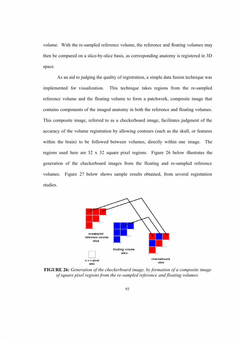
8/12/2019 Jeremy Nett
http://slidepdf.com/reader/full/jeremy-nett 108/124
93
volume. With the re-sampled reference volume, the reference and floating volumes may
then be compared on a slice-by-slice basis, as corresponding anatomy is registered in 3D
space.
As an aid to judging the quality of registration, a simple data fusion technique was
implemented for visualization. This technique takes regions from the re-sampled
reference volume and the floating volume to form a patchwork, composite image that
contains components of the imaged anatomy in both the reference and floating volumes.
This composite image, referred to as a checkerboard image, facilitates judgment of the
accuracy of the volume registration by allowing contours (such as the skull, or features
within the brain) to be followed between volumes, directly within one image. The
regions used here are 32 x 32 square pixel regions. Figure 26 below illustrates the
generation of the checkerboard images from the floating and re-sampled reference
volumes. Figure 27 below shows sample results obtained, from several registration
studies.
FIGURE 26: Generation of the checkerboard image, by formation of a composite imageof square pixel regions from the re-sampled reference and floating volumes.
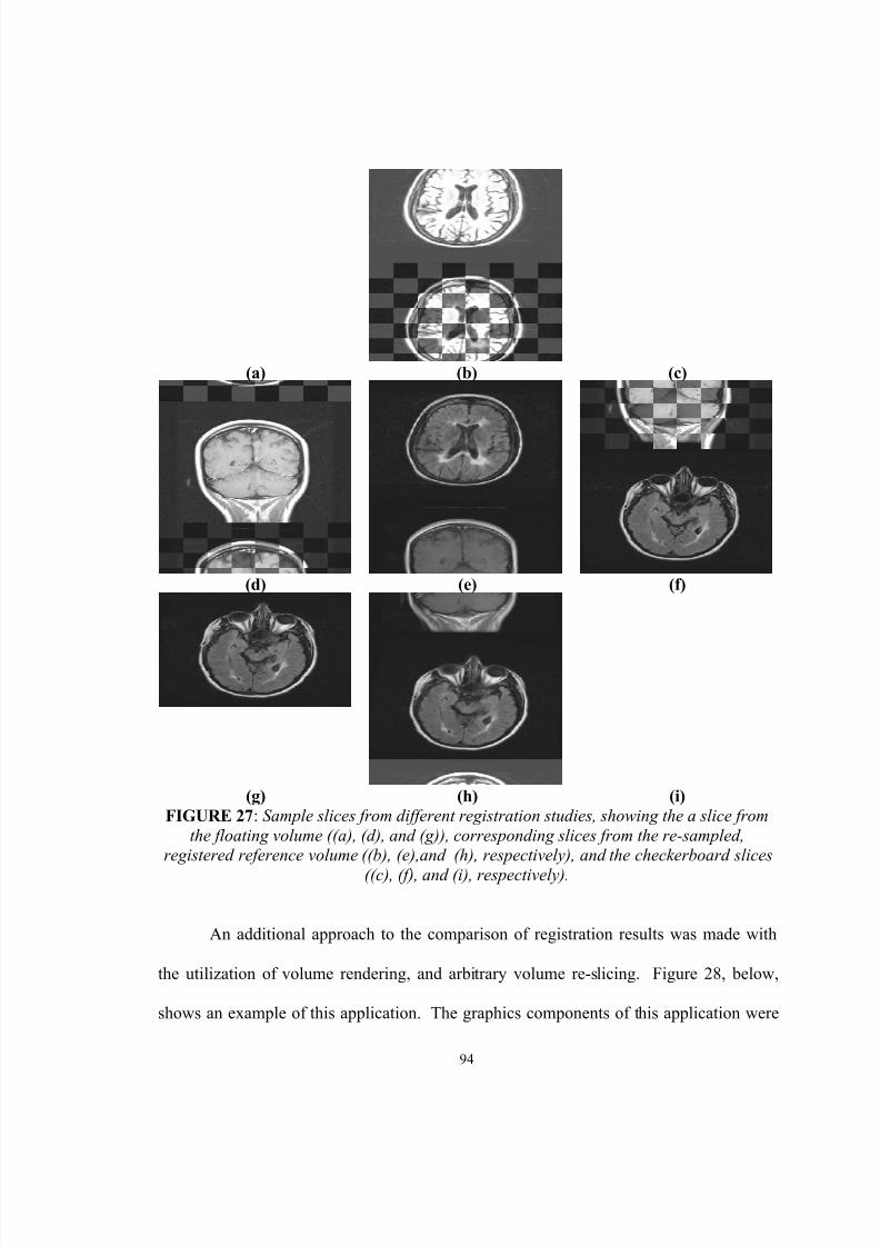
8/12/2019 Jeremy Nett
http://slidepdf.com/reader/full/jeremy-nett 109/124
94
(a) (b) (c)
(d) (e) (f)
(g) (h) (i)FIGURE 27 : Sample slices from different registration studies, showing the a slice from
the floating volume ((a), (d), and (g)), corresponding slices from the re-sampled,registered reference volume ((b), (e),and (h), respectively), and the checkerboard slices
((c), (f), and (i), respectively).
An additional approach to the comparison of registration results was made with
the utilization of volume rendering, and arbitrary volume re-slicing. Figure 28, below,
shows an example of this application. The graphics components of this application were
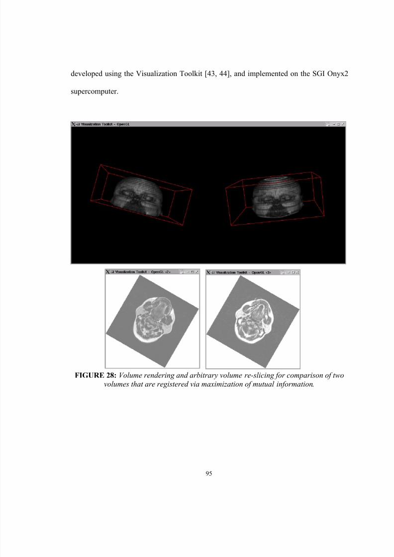
8/12/2019 Jeremy Nett
http://slidepdf.com/reader/full/jeremy-nett 110/124
95
developed using the Visualization Toolkit [43, 44], and implemented on the SGI Onyx2
supercomputer.
FIGURE 28: Volume rendering and arbitrary volume re-slicing for comparison of twovolumes that are registered via maximization of mutual information .
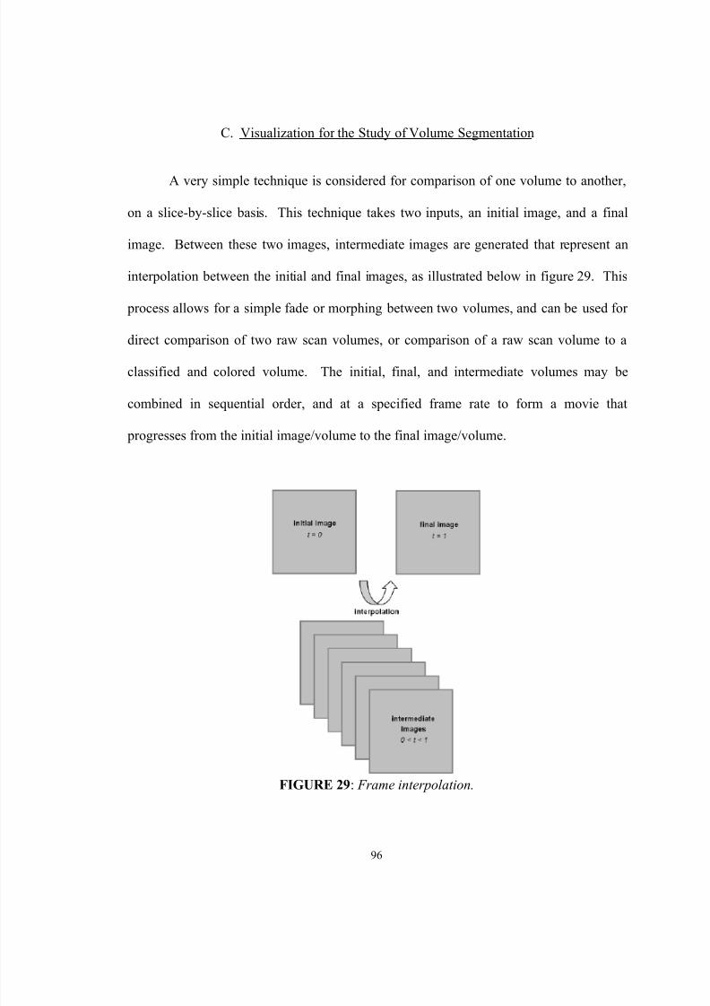
8/12/2019 Jeremy Nett
http://slidepdf.com/reader/full/jeremy-nett 111/124
96
C. Visualization for the Study of Volume Segmentation
A very simple technique is considered for comparison of one volume to another,
on a slice-by-slice basis. This technique takes two inputs, an initial image, and a final
image. Between these two images, intermediate images are generated that represent an
interpolation between the initial and final images, as illustrated below in figure 29. This
process allows for a simple fade or morphing between two volumes, and can be used for
direct comparison of two raw scan volumes, or comparison of a raw scan volume to a
classified and colored volume. The initial, final, and intermediate volumes may be
combined in sequential order, and at a specified frame rate to form a movie that
progresses from the initial image/volume to the final image/volume.
FIGURE 29 : Frame interpolation.
8/12/2019 Jeremy Nett
http://slidepdf.com/reader/full/jeremy-nett 112/124
97
The interpolation scheme implemented in this research consists of interpolation
on a sample to sample basis. Thus, a sample from the initial image is interpolated until
the sample in the corresponding location in the final image is reached, independent of the
other samples in the image/volume.
Simple linear interpolation from a sample x 0 to x 1 is given in eq. 40, below. The
interpolated value, x(t), is a function of time t, a parameter for ordering the interpolated
images/volumes. The time parameter will range from 0, which generates the initial value
x0, to 1, which generates the final value x 1.
001 )()( xt x xt x +⋅−= (40)
The above interpolation scheme may be generalized, by a time-dependent kernel
function k(t), other than t. Eq. 41 below generalizes the interpolation given in eq. 40.
001 )()()( xt k x xt x +⋅−= (41)
Different kernel functions, including exponential, and quadratic functions were
experimented with. Kernels, such as an exponential function, with less abrupt transitions

8/12/2019 Jeremy Nett
http://slidepdf.com/reader/full/jeremy-nett 113/124
98
from zero to one were found to produce the most visually appealing results, in
comparison to a linear interpolation scheme such as eq. 40.
For input and/or output images that are color, interpolation for each sample is
performed on the color components of the samples, using a red, green, blue (RGB) color
parameterization.
D. Web-Based Presentation of Results
Finally, web-based presentation of results was implemented, for presentation of
the results on the Internet. Therefore, the results may be viewed and evaluated from
virtually anyplace in the world (anyplace with Internet access available, at least). Figure
30 below shows an example of one of the web pages that was created for this presentation
format.
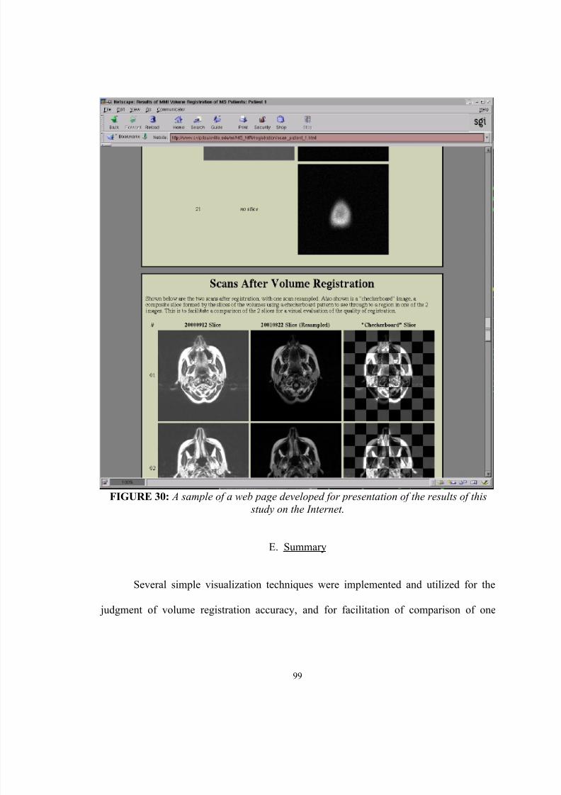
8/12/2019 Jeremy Nett
http://slidepdf.com/reader/full/jeremy-nett 114/124
99
FIGURE 30: A sample of a web page developed for presentation of the results of this study on the Internet .
E. Summary
Several simple visualization techniques were implemented and utilized for the
judgment of volume registration accuracy, and for facilitation of comparison of one

8/12/2019 Jeremy Nett
http://slidepdf.com/reader/full/jeremy-nett 115/124
100
volume to another. These techniques are simple, but useful, and form groundwork for
more involved visualization to be applied for the study of MS.

8/12/2019 Jeremy Nett
http://slidepdf.com/reader/full/jeremy-nett 116/124
101
VI. CONCLUSIONS AND RECOMMENDATIONS
The components of the preliminary system for the study of MS using MRI include
registration for volumetric alignment of patient studies over the course of time, brain
segmentation from the head facilitated by the use of registration, segmentation and
classification of brain tissue to the three tissue classes: CSF, normal brain material, and
diseased brain material, and the use of scientific visualization for the comparison of
patient scans and validation of the registration and segmentation processing.
While additional follow-up work is necessary, the developed approaches provide
a solid foundation on which to build future development in the study of MS using MRI,
as well as to future studies in medical imaging.
Based on the research and development implemented in this thesis, the following
recommendations for future work are made:
• For better volumetric registration, enhancement of the mutual
information approach to incorporate additional features into the registration
for better spatial alignment [39], improvement in the metric itself [40], and
perhaps incorporation of non-rigid body registration[41]. The results
obtained for registration here are useful, however, there is room for
improvement.
• For improved brain segmentation from the head, exploration of
techniques to directly segment the brain, or further development of the
registration approach explored here, to incorporate a high resolution, expert-
8/12/2019 Jeremy Nett
http://slidepdf.com/reader/full/jeremy-nett 117/124
102
segmented model of the head, to provide the a priori segmentation. The
results obtained here show that the registration approach can be useful,
however, manual segmentation of the brain for an a priori segmented model
is far from ideal for use in a large scale study.
• For improvement in the segmentation/classification of the extracted
brain material into CSF, normal brain tissue, and diseased brain tissue, a
means of correcting for inter-intensity variation in the MRI. The wide
variation in intensity levels encountered from the data available to this
research negates any possibility of application of a statistical classification
technique based upon training data from a slice.
• For automation in the segmentation/classification of the extracted
brain material, generation of training data automatically. It is hypothesized
that by use of a filter (such as the non-linear anisotropic diffusion filter
applied in other areas here), an unsupervised classification algorithm (such as
the k-means clustering algorithm studied here), and a rule set, that generation
of training data may be possible. Inter- and intra-slice intensity correction
would assist in this effort, as well.
• From an intensity-corrected study, and automated generation of
training data, 3D segmentation of lesions from the brain is possible, allowing
for more complex, 3D visualization tools to be applied for qualitative
discovery.
• For multiple scans of a patient, taken at different time points, it may

8/12/2019 Jeremy Nett
http://slidepdf.com/reader/full/jeremy-nett 118/124
103
be possible to use previous scans, prior to a given time, to improve in the
future segmentation and classification of brain material into CSF, normal
brain tissue, and diseased brain tissue. This would allow for, if for nothing
else, providing an initial solution for an iterative approach, and possibly
assisting in generating training data.
• Improved quantification of error in the registration and segmentation
processing. At the present, the judgment of quality of the registration and
segmentation procedures largely depends upon qualitative evaluation by an
expert; it would be useful to quantify these errors numerically.
8/12/2019 Jeremy Nett
http://slidepdf.com/reader/full/jeremy-nett 119/124
104
REFERENCES
[1] J. H. Noseworthy, C. Lucchinetti, M. Rodriguez, and B. G. Weinshenker,“Multiple sclerosis,” The New England Journal of Medicine, vol. 343, no. 13, pp.938-952, Sept. 28, 2000.
[2] National Institutes of Neurological Disorders and Stroke, “Multiple Sclerosis:Hope Through Research,” NIH Publication No. 96-75, July 1, 2001.
[3] Z. P. Liang and P. C. Lauterbur, Principles of Magnetic Resonance Imaging: ASignal Processing Perspective. New York: IEEE Press, 2000.
[4] D. H. Miller, P. S. Albert, F. Barkhof, G. Francis, J. A. Frank, S. Hodgkinson, F.D. Liblin, D. W. Paty, S. C. Reingold, and J. Simon, “Guidelines for the Use ofMagnetic Resonance Techniques in Monitoring the Treatment of MultipleSclerosis,” Annals of Neurology, vol. 39, no. 1, Jan. 1996.
[5] C. R. G. Guttmann, R. Kikinis, M. C. Anderson, M. Jakab, S. K. Warfield, R. J.Killiany, H. L. Weiner, F. A. Jolesz, “Quantitative Follow-up of Patients withMultiple Sclerosis: Reproducibility,” JMRI, vol. 9, no. 4., pp. 509-518, June1999.
[6] R. Kikinis, C. R. G. Guttmann, D. Metcalf, W. M. Wells, G. J. Ettinger, H. L.Weiner, and F. A. Jolesz, “Quantitative Follow-up of Patients with MultipleSclerosis: Technical Aspects,” JMRI, vol. 9, no. 4, pp. 519-530, June 1999.
[7] W. M. Wells, W. E. L. Grimson, R. Kikinis, and F. A. Jolesz, “AdaptiveSegmentation of MRI Data,” IEEE Transactions on Medical Imaging, vol. 15, no.4, pp. 429-442, August 1996.
[8] M. Kamber, R. Shinghal, D. L. Collins, G. S. Francis, and A. C. Evans, “Model-Based 3-D Segmentation of Multiple Sclerosis Lesions in Magnetic ResonanceBrain Images,” IEEE Transactions on Medical Imaging, vol. 14., no. 3, pp. 442-453, Sept. 1995.
8/12/2019 Jeremy Nett
http://slidepdf.com/reader/full/jeremy-nett 120/124
105
[9] B. Johnston, M. S. Atkins, B. Mackiewich, and M. Anderson, “Segmentation ofMultiple Sclerosis Lesions in Intensity Corrected Multispectral MRI,” IEEETransactions on Medical Imaging, vol. 15, no. 2, pp. 154-169, April 1996.
[10] J. Besag, “On the Statistical Analysis of Dirty Pictures,” Journal of the RoyalStatistical Society B, vol. 48, no. 3, pp. 259-30, 1986.
[11] J. K. Udupa, L. Wei, S. Samarasekera, Y. Miki, M. A. van Buchem, and R. I.Grossman, “Multiple Sclerosis Lesion Quantifiction Using Fuzzy-ConnectednessPrinciples,” IEEE Transactions on Medical Imaging, vol. 16, no. 5, pp. 598-609,Oct. 1997.
[12] J. K. Udupa and S. Samarasekera, “Fuzzy Connectedness and Object Definition:Theory, Algorithms, and Applications in Image Segmentation,” Graphical Modelsand Image Processing, vol. 58, no. 3, pp. 246-261, May 19996.
[13] K. V. Leemput, F. Maes, D. Vandermeulen, A. Colchester, and P. Suetens,“Automated Segmentation of Multiple Sclerosis Lesions by Model OutlierDetection,” IEEE Transactions on Medical Imaging, vol. 20, no. 8, pp. 677-688,August 2001.
[14] F. Maes, A. Collignon, D. Vandermeulen, G. Marchal, and P. Suetens,“Multimodality Image Registration by Maximization of Mutual Information,”IEEE Transactions on Medical Imaging, vol. 16, no. 2, pp. 187-198, April 1997.
[15] W. M. Wells, P. Viola, H. Atsumi, S. Nakajima, and R. Kikinis, “Multi-modalVolume Registration by Maximization of Mutual Information,” Medical ImageAnalysis, vol. 1, no. 1, pp. 35-51, 1996.
[16] C. R. Meyer, J. L. Boes, B. Kim, P. H. Bland, K. R. Zasadny, P. V. Kison, K.Koral, K. A. Frey, and R. L. Wahl, “Demonstration of Accuracy and ClinicalVersatility of Mutual Information for Automatic Multimodality Image FusionUsing Affine and Thin-Plate Spline Warped Geometric Deformations,” MedicalImage Analysis, vol. 1., no. 3, pp. 195-206, 1996/7.
8/12/2019 Jeremy Nett
http://slidepdf.com/reader/full/jeremy-nett 121/124
106
[17] J. Nolte, The Human Brain: An Introduction to its Functional Anatomy. St.Louis: Mosby Year Book, 3 rd edition, 1993.
[18] J. B. A. Maintz and M. A. Viergever, “A Survey of Medical Image Registration,”Medical Image Analysis, vol. 2., no. 1, pp. 1-36, 1998.
[19] M. A. Audette, F. P. Ferrie, and T. M. Peters, “An Algorithmic Overview ofSurface Registration Techniques for Medical Imaging,” Medical Image Analysis,vol. 4, pp. 201-217, 2000.
[20] G. Wolberg, Digital Image Warping. Los Alamitos: IEEE Computer SocietyPress, 1990.
[21] T. M. Cover and J. A. Thomas, Elements of Information Theory. New York:John Wiley & Sons, 1991.
[22] G. P. Penney, J. Weese, J. A. Little, P. Desmedt, D. L. G. Hill, and D. J. Hawkes,“A Comparison of Similarity Measures for Use in 2D-3D Medical ImageRegistration,” IEEE Transactions on Medical Imaging, vol. 17, no. 4, pp. 586-595, August 1998.
[23] W. H. Press, S. A. Teukolsky, W. T. Vetterling, and B. P. Flannery, NumericalRecipes in C: The Art of Scientific Computing. Cambridge University Press,Second Edition, 1992.
[24] F. Maes, D. Vandermeulen, and P. Suetens, “Comparative Evaluation ofMultiresolution Optimization Strategies for Multimodality Image Registration byMaximization of Mutual Information,” Medical Image Analysis, vol. 3, no. 4, pp.373-386, 1999.
[25] S. L. S. Jacoby, J. S. Kowalik, and J. T. Pizzo, Iterative Methods for NonlinearOptimization Problems. Englewood Cliffs: Prentice-Hall, 1972.
8/12/2019 Jeremy Nett
http://slidepdf.com/reader/full/jeremy-nett 122/124
107
[26] M. Joliet and B. M. Mazoyer, “Three-Dimensional Segmentation andInterpolation of Magnetic Resonance Brain Images,” IEEE Transactions onMedical Imaging, vol. 12, no. 2, pp. 269-277, June 1993.
[27] M. E. Brummer, R. M. Mersereau, R. L. Eisner, and R. R. J. Lewine, “AutomaticDetection of Brain Contours in MRI Data Sets,” IEEE Transactions on MedicalImaging, vol. 12, no. 2, pp. 153-166, June 1993.
[28] T. Kapur, W. E. L. Grimson, W. M. Wells, and R. Kikinis, “Segmentation ofBrain Tissue from Magnetic Resonance Images,” Medical Image Analysis, vol. 1,no. 2, pp. 109-127, 1996.
[29] M. S. Atkins and B. T. Mackiewich, “Fully Automatic Segmentation of the Brainin MRI,” IEEE Transactions on Medical Imaging, vol. 17, no. 1, pp. 98-107, Feb.1998.
[30] C. Sites, A. Farag, and T. Moriarty, “Visualization Algorithms for MedicalImaging with Telemedicine and High Performance Computing Applications,”Technical Report, CVIP Laboratory, December 2000.
[31] N. Shareef, D. L. Wang, and R. Yagel, “Segmentation of Medical Images UsingLEGION,” IEEE Transactions on Medical Imaging, vol. 18, no. 1, pp. 74-91, Jan.1999.
[32] G. Gerig, O. Kübler, R. Kikinis, and F. A. Jolesz, “Nonlinear AnisotropicFiltering of MRI Data,” IEEE Transactions on Medical Imaging, vol. 11, no. 2,
pp. 221-232, June 1992.
[33] R. O. Duda, P. E. Hart, and D. G. Stork, Pattern Classification. New York: JohnWiley & Sons, 2 nd edition, 2001.
[34] H. E. Cline, W. E. Lorensen, R. Kikinis, and F. Jolesz, “Three-DimensionalSegmentation of MR Images of the Head Using Probability and Connectivity,”Journal of Computer Assisted Tomography, vol. 14, no. 6, pp. 1037-1045,
November/December 1990.
8/12/2019 Jeremy Nett
http://slidepdf.com/reader/full/jeremy-nett 123/124
108
[35] R. V. Hogg and E. A. Tanis, Probability and Statistical Inference. Upper SaddleRiver: Prentice-Hall, 6 th edition, 2001.
[36] S. Z. Li, Markov Random Field Modeling in Image Analysis. Tokyo: Springer-Verlag, 2001
[37] K. Held, E. R. Kops, B. J. Krause, W. M. Wells, R. Kikinis, and H. W. Müller-Gärtner, “Markov Random Field Segmentation of Brain MR Images,” IEEETransactions on Medical Imaging, vol. 16, no. 6, pp. 878-886, Dec. 1997.
[38] C. W. Therrien, Decision, Estimation, and Classification. New York: John Wiley& Sons, 1989.
[39] J. P. W. Pluim, J. B. A. Maintz, and M. A. Viergever, “Image Registration byMaximization of Combined Mutual Information and Gradient Information,” IEEETransactions on Medical Imaging, vol. 19, no. 8, pp. 809-814, August 2000.
[40] C. Studholme, D. L. G. Hill, and D. J. Hawkes, “An Overlap Invariant EntropyMeasure of 3D Medical Image Alignment,” Pattern Recognition, vol. 32, pp. 71-86, 1999.
[41] B. Likar and F. Pernus, “A Hierarchical Approach to Elastic Registration Basedon Mutual Information,” Image and Vision Computing, vol. 19, pp. 33-44, 2001.
[42] American College of Radiology, National Electrical Manufacturers Association,"Digital Imaging and Communications in Medicine (DICOM): Version 3.0",Draft Standard, ACR-NEMA Committee, Working Group VI, Washington, DC,1993.
[43] W. J. Schroeder, L. S. Avila, K. M. Martin, W. A. Hoffman, and C. C. Law, TheVTK User’s Guide. Kitware, 2001.
[44] W. Schroeder, K. Martin, and B. Lorensen, The Visualization Toolkit: An Object-Oriented Approach to 3D Graphics. Upper Saddle River: Prentice-Hall, 2 nd Edition, 1998.
8/12/2019 Jeremy Nett
http://slidepdf.com/reader/full/jeremy-nett 124/124
VITA
Jeremy Michael Nett, son of Michael and Kathy Nett, was born on July 9, 1978 in
Louisville, Kentucky. He graduated as class valedictorian from Tates Creek High School
in Lexington, Kentucky, in 1996. In the fall of 1996, he entered the Speed Scientific
School at the University of Louisville. In spring of 2000, he graduated summa cum laude
from the University of Louisville with a Bachelor of Science degree in Electrical
Engineering. During his undergraduate studies, he completed three co-operative
internships with Thomson Consumer Electronics, in Indianapolis, IN. In the summer of
2000, he began his studies towards a Masters of Engineering degree at the University of
Louisville's Computer Vision and Image Processing Lab, in the Electrical and Computer
Engineering Department.