Is production system important for

survival times after first calving of

dairy cows?

Supervisor: Lars Rönnegård

Author: JIA ZHAO

Department of Economics and Social Science, Dalarna University

D-level essay in Applied Statistics, 2009

1

Contents

Abstract ……………………………………………………………………………... 1

1. Introduction ……………………………………………………………………… 2

2. Data ……………………………………………………………………………….. 5

2.1 Data pretreatment ................................................................................................ 5

2.2 Data description ....................................................................................................7

3. Methodology ……………………………………………………………………... 8

3.1 Survival Analysis ……………………………………………………………….. 8

3.1.1 Non-parametric survival model ........................................................................8

3.1.1.1 Kaplan-Meier estimator ……………………………………………………. 8

3.1.1.2 Log-rank test ………………………………………………………………... 9

3.1.1.3 Cox proportional hazard model …………………………………………… 9

3.1.2 Parametric survival model …………………………………………………. 10

3.2 Generalized Linear Model ……………………………………………………. 11

3.2.1 Maximum Likelihood Estimation ………………………………………….. 11

3.2.2 Weibull distribution ………………………………………………………… 12

3.3 Adding random effect …………………………………………………………. 12

4. Result ……………………………………………………………………………. 13

4.1 Kaplan-Meier estimator and log-rank test …………………………………... 13

4.2 Cox proportional hazard model and frailty model …………………………. 14

4.3 Parametric survival model (with and without random effect) ……………... 15

4.4 GLM and GLMM ……………………………………………………………... 15

5. Conclusion ………………………………………………………………………. 16

6. Discussion ……………………………………………………………………….. 17

Reference …………………………………………………………………………... 19

Appendix …………….. …………………………………………………………… 20

2

Abstract

The survival times of dairy cows after first calving as a part of animal welfare has

attracted broad attention. In this article the main objective is to find whether the

difference of production systems can affect the survival times after first calving; the

sub objective is to apply different methods to solve this problem. We solve this

problem from two directions: Survival Analysis and a Generalized Linear model

approach. The Survival Analysis includes both Cox proportional hazard model and a

parametric survival model. Then “herd effect” is added as a random effect to all three

models. After model regression the results of all models which are without or with

random effect show the organic production system has a higher survival rate than the

traditional production system. After adding the herd effect, the higher survival rate of

organic production system becomes more significant in all three models. Modelling of

individuals’ relationship is also discussed.

Key words: dairy cows, survival times after first calving, Survival Analysis, Cox

proportional hazard model, parametric survival model, Generalized Linear model,

random effect

3

1. Introduction

Dairy cows are domesticated animals bred to produce milk. A cow will produce large

amounts of milk over its life after first calving which is a precondition of milking.

Common gestation period of cows is about nine months, so most heifers (cows before

first calving) give birth and become cows at about two years of age. There are many

kinds of dairy cows. Certain breeds produce more milk than others; however, different

breeds produce within a range of around 4,000 to over 10,000 kg of milk per annum.

Production levels peak at around 40 to 60 days after calving. The cow is then bred.

Production declines steadily afterwards, until, at about 305 days after calving, the cow

is “dried off”, and milking ceases. About sixty days later, one year after the birth of

her previous calf (baby), a cow will calve again. High production cows are more

difficult to breed at a one year interval. Many farms take the view that 13 or even 14

month cycles are more appropriate for this type of cow1.

In Sweden Swedish Red and White Cattle are the most common dairy cows and the

population of this breed is 60% of the total number. Besides this breed there are still

seven breeds in Sweden shown below. Swedish Holstein Friesian Cattle, which are

characterized by a high milk yield, are the second large breeds of dairy cows in

Sweden. And also some breeds of small size groups such as Swedish Red Polled

Cattle, Bohus Poll Cattle, Ringamala Cattle, Vane Cattle, Fjall Cattle and

Swedish Mountain Cattle2.

Swedish Red and Swedish Holstein Red Polled Cattle Bohus Poll Cattle

White Cattle Friesian Cattle

Ringamala Cattle Vane Cattle Fjall Cattle Swedish Mountain Cattle

Figure 1 Breeds of dairy cows in Sweden.

The dairy sector is the most important sector in Swedish agriculture today. The main

dairy products in Sweden are drinking milk, fermented milk, cream, cheese, butter

and milk powder. In total, there are 15 dairy companies in Sweden. Seven of them are

1 http://en.wikipedia.org/wiki/Dairy_cattle

2 http://neurocad.lva.lt/Breeds/SwedishBreeds.htm

4

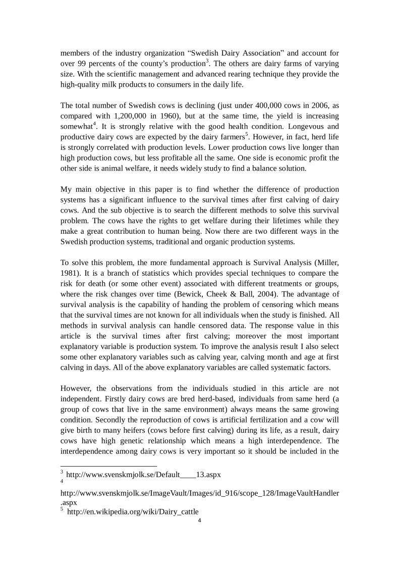
members of the industry organization “Swedish Dairy Association” and account for

over 99 percents of the county’s production3. The others are dairy farms of varying

size. With the scientific management and advanced rearing technique they provide the

high-quality milk products to consumers in the daily life.

The total number of Swedish cows is declining (just under 400,000 cows in 2006, as

compared with 1,200,000 in 1960), but at the same time, the yield is increasing

somewhat4. It is strongly relative with the good health condition. Longevous and

productive dairy cows are expected by the dairy farmers5. However, in fact, herd life

is strongly correlated with production levels. Lower production cows live longer than

high production cows, but less profitable all the same. One side is economic profit the

other side is animal welfare, it needs widely study to find a balance solution.

My main objective in this paper is to find whether the difference of production

systems has a significant influence to the survival times after first calving of dairy

cows. And the sub objective is to search the different methods to solve this survival

problem. The cows have the rights to get welfare during their lifetimes while they

make a great contribution to human being. Now there are two different ways in the

Swedish production systems, traditional and organic production systems.

To solve this problem, the more fundamental approach is Survival Analysis (Miller,

1981). It is a branch of statistics which provides special techniques to compare the

risk for death (or some other event) associated with different treatments or groups,

where the risk changes over time (Bewick, Cheek & Ball, 2004). The advantage of

survival analysis is the capability of handing the problem of censoring which means

that the survival times are not known for all individuals when the study is finished. All

methods in survival analysis can handle censored data. The response value in this

article is the survival times after first calving; moreover the most important

explanatory variable is production system. To improve the analysis result I also select

some other explanatory variables such as calving year, calving month and age at first

calving in days. All of the above explanatory variables are called systematic factors.

However, the observations from the individuals studied in this article are not

independent. Firstly dairy cows are bred herd-based, individuals from same herd (a

group of cows that live in the same environment) always means the same growing

condition. Secondly the reproduction of cows is artificial fertilization and a cow will

give birth to many heifers (cows before first calving) during its life, as a result, dairy

cows have high genetic relationship which means a high interdependence. The

interdependence among dairy cows is very important so it should be included in the

3 http://www.svenskmjolk.se/Default____13.aspx

4

http://www.svenskmjolk.se/ImageVault/Images/id_916/scope_128/ImageVaultHandler

.aspx 5 http://en.wikipedia.org/wiki/Dairy_cattle

5

analysis. Both of them should be treated as random effects to improve survival models

and make them have the ability of capturing the comovement of survival times among

dairy cows. As we know Generalized Linear Model with random effect is commonly

referred to as Generalize Linear Mixed Model (Fahrmeir & Tutz, 2001) in the

statistical literature. And I also add random effect to the models of survival analysis

and then compare the results of these different models.

All models have their own predominance. I will make a discussion after I apply them

to the model regressions.

2. Data

The data in my article is provided by “Swedish Dairy Association” which belongs to

the seven largest companies (jointly representing more than 99 percents of Swedish

milk production), seven livestock cooperatives, two semen-producing companies, and

nine breed societies. The work of this association covers ten different fields of

expertise including “Nutrition & Gastronomy”, “Milk Quality”, “Environmental

Issues”, “Milk Police”, “Milk Economy”, “Management”, “Cow Data”, “Breeding”,

“Animal Welfare”, “and Breeding”. Today it has been a company with a

well-established network of researchers, experts, decision-makers, and people who

shape public opinions, in Sweden and abroad6.

2.1 Data pretreatment

The complete data is recorded from January 1998 to September 2005. We select the

individuals who had their first calving during year 1998 to year 1999. After this

selection, there are 129760 individuals included in the dataset which come from 9295

different herds. In the methodology part “herd” will be treated as a random effect

which has a 𝑛 × 𝑛 matrix form (here n=9295). It is too large to calculate for R

software used in this article. To solve this problem I delete some observations to make

the size of each herd more than or equal to 10 heads. Then the total number of herds

reduced to 4769 (almost decreased 50%) which can be calculate by R in practice. At

the same time the total number of observations is reduced to 109986 (almost

decreased 15%) which is also large enough for modelling and analysis.

The dataset after selected by “herd” also incorporates information of individuals

which consists some indirect and unnecessary information. So I must do some

pre-treatments before I use them.

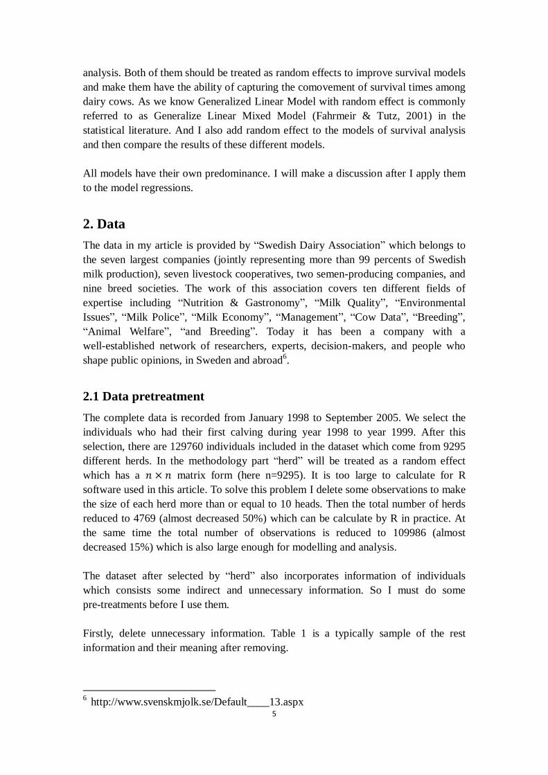
Firstly, delete unnecessary information. Table 1 is a typically sample of the rest

information and their meaning after removing.

6 http://www.svenskmjolk.se/Default____13.aspx

6

Table 1 Data after removing unnecessary information. (First three rows of

observations.)

calvyr calvmo age Utslagskod utslagsdatum Herd Calvingdate System

1998 1 809 3 15131 100 13896 0

1998 3 821 4 15472 100 13953 0

1999 8 894

107 14465 0

calvyr: year of first cavling calvmo: month of first calving

age: age of cows at first calving in days Utslagskod: reason of death

utslagsdatum: date of death Herd: herd the cow belongs to

Calvingdate: data of first calving System: traditional=0 organic=1

Secondly, calculate the survival times after first calving. There are pair wise missing

values in date of death and death reason which means the cows are still alive until

September 2005. Then I define a new group of data named “state” which have two

values 1 and 0; 1 means the individual is dead and 0 means it is still alive after

September 2005. The date of September 2005 is 16700 which I treat it as the date of

death. The survival times of this kind of individuals are censored data7.

Thirdly, make a final check. Survival times must be nonnegative in actual life but

some values are negative in the dataset. So I delete them. After all of procedures I get

the final dataset. Table 2 shows the final dataset after all above treatments.

Table 2 Final model form (First three rows of observations.)

time state calvyr calvmo age herd system

1235 1 1998 1 809 100 0

1519 1 1998 3 821 100 0

2235 0 1999 8 894 107 0

time: survival time after first calving state: dead=1 alive=0

calvyr: year of first cavling calvmo: month of first calving

age: age of cows at first calving in days herd: herd the cow belongs to

system: traditional=0 organic=1

7 http://en.wikipedia.org/wiki/Censoring_(statistics)

7

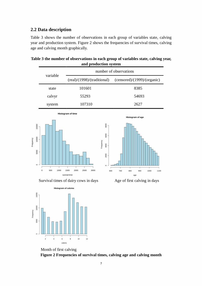
2.2 Data description

Table 3 shows the number of observations in each group of variables state, calving

year and production system. Figure 2 shows the frequencies of survival times, calving

age and calving month graphically.

Table 3 the number of observations in each group of variables state, calving year,

and production system

variable number of observations

(real)/(1998)/(traditional) (censored)/(1999)/(organic)

state 101601 8385

calvyr 55293 54693

system 107310 2627

Survival times of dairy cows in days Age of first calving in days

Month of first calving

Figure 2 Frequencies of survival times, calving age and calving month

Histogram of time

survival time

Fre

qu

en

cy

0 500 1000 1500 2000 2500 3000

05

00

01

00

00

15

00

0

Histogram of age

age

Fre

qu

en

cy

600 700 800 900 1000 1100

02

00

04

00

06

00

08

00

0

Histogram of calvmo

calvmo

Fre

qu

en

cy

2 4 6 8 10 12

05

00

01

00

00

15

00

0

8

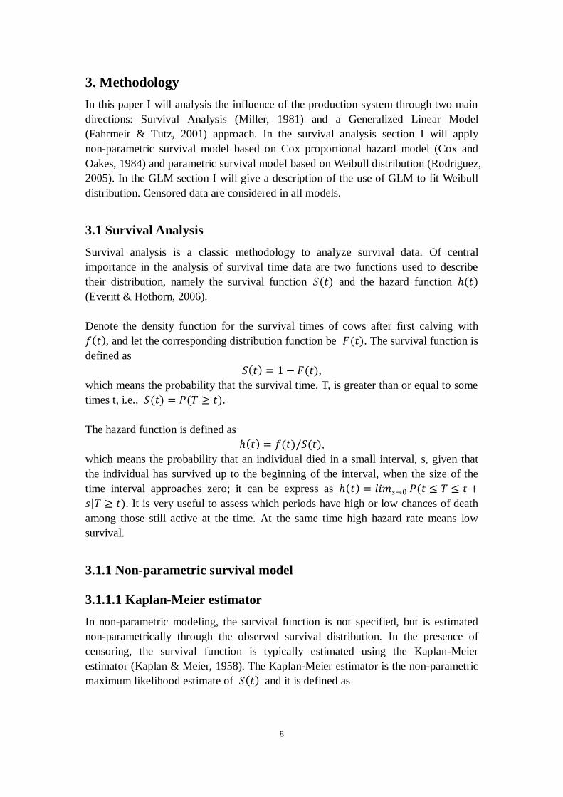
3. Methodology

In this paper I will analysis the influence of the production system through two main

directions: Survival Analysis (Miller, 1981) and a Generalized Linear Model

(Fahrmeir & Tutz, 2001) approach. In the survival analysis section I will apply

non-parametric survival model based on Cox proportional hazard model (Cox and

Oakes, 1984) and parametric survival model based on Weibull distribution (Rodriguez,

2005). In the GLM section I will give a description of the use of GLM to fit Weibull

distribution. Censored data are considered in all models.

3.1 Survival Analysis

Survival analysis is a classic methodology to analyze survival data. Of central

importance in the analysis of survival time data are two functions used to describe

their distribution, namely the survival function 𝑆(𝑡) and the hazard function 𝑕(𝑡)

(Everitt & Hothorn, 2006).

Denote the density function for the survival times of cows after first calving with

𝑓 𝑡 , and let the corresponding distribution function be 𝐹(𝑡). The survival function is

defined as

𝑆 𝑡 = 1 − 𝐹(𝑡),

which means the probability that the survival time, T, is greater than or equal to some

times t, i.e., 𝑆(𝑡) = 𝑃(𝑇 ≥ 𝑡).

The hazard function is defined as

𝑕 𝑡 = 𝑓(𝑡)/𝑆(𝑡),

which means the probability that an individual died in a small interval, s, given that

the individual has survived up to the beginning of the interval, when the size of the

time interval approaches zero; it can be express as 𝑕 𝑡 = 𝑙𝑖𝑚𝑠→0 𝑃(𝑡 ≤ 𝑇 ≤ 𝑡 +

𝑠 𝑇 ≥ 𝑡 ). It is very useful to assess which periods have high or low chances of death

among those still active at the time. At the same time high hazard rate means low

survival.

3.1.1 Non-parametric survival model

3.1.1.1 Kaplan-Meier estimator

In non-parametric modeling, the survival function is not specified, but is estimated

non-parametrically through the observed survival distribution. In the presence of

censoring, the survival function is typically estimated using the Kaplan-Meier

estimator (Kaplan & Meier, 1958). The Kaplan-Meier estimator is the non-parametric

maximum likelihood estimate of 𝑆 𝑡 and it is defined as

9

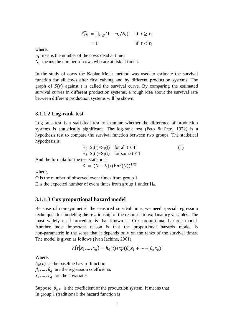
𝑆𝐾𝑀 = (1 − 𝑛𝑖/𝑁𝑖)𝑡𝑖≤𝑡 if 𝑡 ≥ 𝑡𝑖

= 1 if 𝑡 < 𝑡𝑖

where,

𝑛𝑖 means the number of the cows dead at time t

𝑁𝑖 means the number of cows who are at risk at time t.

In the study of cows the Kaplan-Meier method was used to estimate the survival

function for all cows after first calving and by different production systems. The

graph of 𝑆(𝑡) against t is called the survival curve. By comparing the estimated

survival curves in different production systems, a rough idea about the survival rate

between different production systems will be shown.

3.1.1.2 Log-rank test

Log-rank test is a statistical test to examine whether the difference of production

systems is statistically significant. The log-rank test (Peto & Peto, 1972) is a

hypothesis test to compare the survival function between two groups. The statistical

hypothesis is

H0: S1(t)=S2(t) for all t T (1)

H1: S1(t)S2(t) for some t T

And the formula for the test statistic is

𝑍 = (𝑂 − 𝐸)/(𝑉𝑎𝑟(𝑂))1/2

where,

O is the number of observed event times from group 1

E is the expected number of event times from group 1 under H0.

3.1.1.3 Cox proportional hazard model

Because of non-symmetric the censored survival time, we need special regression

techniques for modeling the relationship of the response to explanatory variables. The

most widely used procedure is that known as Cox proportional hazards model.

Another most important reason is that the proportional hazards model is

non-parametric in the sense that it depends only on the ranks of the survival times.

The model is given as follows (Ivan Iachine, 2001)

𝑕 𝑡 𝑥1,… , 𝑥𝑞 = 𝑕0(𝑡)𝑒𝑥𝑝(𝛽1𝑥1 + ⋯+ 𝛽𝑞𝑥𝑞)

Where,

𝑕0(𝑡) is the baseline hazard function

𝛽1 ,… ,𝛽𝑞 are the regression coefficients

𝑥1,… , 𝑥𝑞 are the covariates

Suppose 𝛽𝑁𝑃 is the coefficient of the production system. It means that

In group 1 (traditional) the hazard function is

10

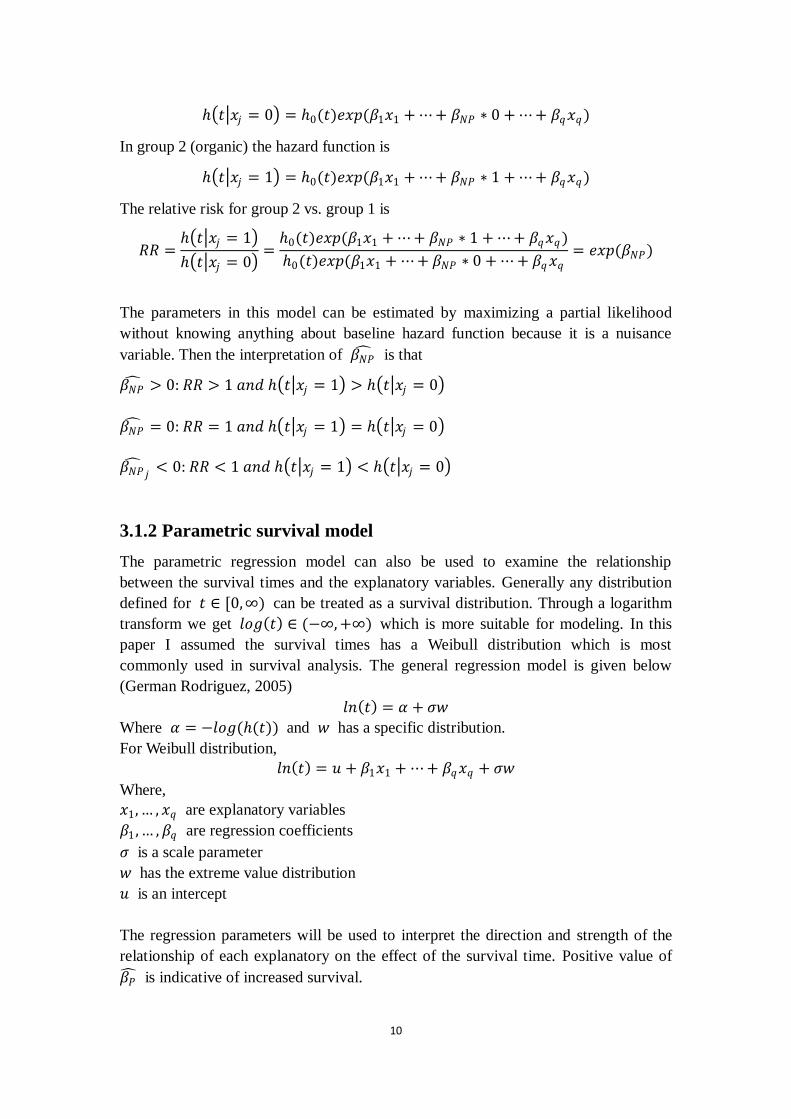
𝑕 𝑡 𝑥𝑗 = 0 = 𝑕0(𝑡)𝑒𝑥𝑝(𝛽1𝑥1 + ⋯+ 𝛽𝑁𝑃 ∗ 0 + ⋯+ 𝛽𝑞𝑥𝑞)

In group 2 (organic) the hazard function is

𝑕 𝑡 𝑥𝑗 = 1 = 𝑕0(𝑡)𝑒𝑥𝑝(𝛽1𝑥1 + ⋯+ 𝛽𝑁𝑃 ∗ 1 + ⋯+ 𝛽𝑞𝑥𝑞)

The relative risk for group 2 vs. group 1 is

𝑅𝑅 =𝑕 𝑡 𝑥𝑗 = 1

𝑕 𝑡 𝑥𝑗 = 0 =𝑕0(𝑡)𝑒𝑥𝑝(𝛽1𝑥1 + ⋯+ 𝛽𝑁𝑃 ∗ 1 + ⋯+ 𝛽𝑞𝑥𝑞)

𝑕0(𝑡)𝑒𝑥𝑝(𝛽1𝑥1 + ⋯+ 𝛽𝑁𝑃 ∗ 0 + ⋯+ 𝛽𝑞𝑥𝑞= 𝑒𝑥𝑝(𝛽𝑁𝑃)

The parameters in this model can be estimated by maximizing a partial likelihood

without knowing anything about baseline hazard function because it is a nuisance

variable. Then the interpretation of 𝛽𝑁𝑃 is that

𝛽𝑁𝑃 > 0: 𝑅𝑅 > 1 𝑎𝑛𝑑 𝑕 𝑡 𝑥𝑗 = 1 > 𝑕 𝑡 𝑥𝑗 = 0

𝛽𝑁𝑃 = 0: 𝑅𝑅 = 1 𝑎𝑛𝑑 𝑕 𝑡 𝑥𝑗 = 1 = 𝑕 𝑡 𝑥𝑗 = 0

𝛽𝑁𝑃 𝑗< 0: 𝑅𝑅 < 1 𝑎𝑛𝑑 𝑕 𝑡 𝑥𝑗 = 1 < 𝑕 𝑡 𝑥𝑗 = 0

3.1.2 Parametric survival model

The parametric regression model can also be used to examine the relationship

between the survival times and the explanatory variables. Generally any distribution

defined for 𝑡 ∈ [0,∞) can be treated as a survival distribution. Through a logarithm

transform we get 𝑙𝑜𝑔 𝑡 ∈ (−∞, +∞) which is more suitable for modeling. In this

paper I assumed the survival times has a Weibull distribution which is most

commonly used in survival analysis. The general regression model is given below

(German Rodriguez, 2005)

𝑙𝑛 𝑡 = 𝛼 + 𝜎𝑤

Where 𝛼 = −𝑙𝑜𝑔(𝑕(𝑡)) and 𝑤 has a specific distribution.

For Weibull distribution,

𝑙𝑛 𝑡 = 𝑢 + 𝛽1𝑥1 + ⋯+ 𝛽𝑞𝑥𝑞 + 𝜎𝑤

Where,

𝑥1,… , 𝑥𝑞 are explanatory variables

𝛽1 ,… ,𝛽𝑞 are regression coefficients

𝜎 is a scale parameter

𝑤 has the extreme value distribution

𝑢 is an intercept

The regression parameters will be used to interpret the direction and strength of the

relationship of each explanatory on the effect of the survival time. Positive value of

𝛽𝑃 is indicative of increased survival.

11

3.2 Generalized Linear Model

Generalized linear model is proposed as a way of unifying various other statistical

models, including linear regression, logistic regression and Poisson regression, under

on framework. It is not common used in the survival analysis but no doubt it will be

an interesting attempt to solve the survival problem with GLM (Aitkin & Clayton,

1979).

3.2.1 Maximum Likelihood Estimation

The hazard function is assumed to involve the explanatory variables through a

log-linear (proportional hazards) model:

𝑕 𝑡𝑖 = 𝜆 𝑡𝑖 𝑒𝑥 𝑝 𝛽𝑗𝑥𝑖𝑗𝑗

= 𝜆 𝑡𝑖 𝑒𝑥𝑝(𝜷′𝒙𝒊)

where,

𝑡1,… , 𝑡𝑛 are the survival times of n individuals

𝑥𝑖𝑗 for 𝑖 = 1,… ,𝑛, and 𝑗 = 0, 1,… , 𝑘 is the explanatory variables with 𝑥𝑖𝑜 ≡ 1

𝛽𝑗 is the regression parameter

Since 𝑕 𝑡 = 𝑓(𝑡)/𝑆(𝑡), the density function 𝑓(𝑡) is assumed to be of the form

𝑓 𝑡 = 𝜆(𝑡)𝑒𝑥𝑝(𝜷′𝒙 − 𝜦(𝑡)𝑒𝜷′ 𝒙), and hence 𝑆 𝑡 = 𝑒𝑥𝑝(−𝜦 𝑡 𝑒𝜷

′𝒙), where

𝜦 𝑡 = 𝜆𝑡

−∞

𝑢 𝑑𝑢

Let 𝑤 be an indicator variable taking the value 1 for uncensored observation and 0

for censored observations. Under the usual assumption that the censoring mechanism

is independent of the explanatory variables, the likelihood function is

𝐿 = 𝑓 𝑡𝑖 𝑤 𝑖 𝑆 𝑡 1−𝑤 𝑖

𝑛

𝑖=1

= 𝜆 𝑡𝑖 𝑒𝑥𝑝(𝜷′𝒙𝒊) 𝑤 𝑖

𝑖 𝑒𝑥𝑝(−𝜦 𝑡 𝑒𝜷′𝒙)

= [𝑢𝑖𝑤 𝑖𝑒−𝑢 𝑖 ]𝑖 [𝜆 𝑡𝑖 /𝜦(𝑡𝑖)]𝑤 𝑖

where 𝑢𝑖 = 𝜦(𝑡𝑖)𝑒𝑥𝑝(𝜷′𝒙𝒊).

The first term in the likelihood function is the kernel of the likelihood function for n

independent “Poisson variates” 𝑤𝑖 with mean 𝑢𝑖 . The second term does not involve

the parameter vector 𝛽, but may depend on other unknow parameters. The log-linear

model for the hazard function implies a log-linear model for the “Poisson mean”

𝑙𝑜𝑔 𝑢𝑖 = 𝑙𝑜𝑔𝜦 𝑡𝑖 + 𝜷′𝒙𝒊

Then a simple iterative maximization of the log-likelihood function is now possible in

12

GLM. Given initial estimates of the unknown parameters in 𝜦 𝑡 , the maximum

likelihood estimate (MLE) of 𝜷 is obtained for the Poisson model in GLM with

log𝜦 𝑡𝑖 as a known function (an offset) incorporated in the log-linear model. For

this estimate of 𝜷, the MLE of the unknown parameters in 𝜦 𝑡 may be obtained

from the likelihood equations for these parameters., and this sequence of steps

continued until convergence.

3.2.2 Weibull distribution

By assuming 𝑡 ≥ 0 and 𝜦 𝑡 = 𝑡𝛼 , we obtain Weibull density

𝑓 𝑡 = 𝛼𝑡𝛼−1𝑒𝑥𝑝(𝜷′𝒙 − 𝑡𝛼𝑒𝜷′ 𝒙), (𝑡 ≥ 0,𝛼 > 0),

with 𝐸 𝑡 = 𝛤(1 + 𝛼−1)𝑒𝑥𝑝(−𝜷′𝒙/𝛼). In this case 𝜆 𝑡 /𝜦 𝑡 = 𝛼/𝑡 will depend

on the unknown shape parameter 𝛼. The kernel of the log-likelihood function is

𝑙𝑜𝑔𝐿 = 𝑛𝑙𝑜𝑔𝛼 + (𝑤𝑖𝑙𝑜𝑔𝑖 𝑢𝑖 − 𝑢𝑖),

where 𝑖 = 1,… ,𝑛 and 𝑙𝑜𝑔 𝑢𝑖 = 𝛼𝑙𝑜𝑔(𝑡𝑖) + 𝜷′𝒙𝒊. The likelihood equations are

𝜕𝑙𝑜𝑔𝐿

𝜕𝛽𝑗= (𝑤𝑖

𝑖− 𝑢𝑖)𝑥𝑖𝑗 = 0

𝜕𝑙𝑜𝑔𝐿

𝜕𝛼= 𝑛/𝛼 + (𝑤𝑖

𝑖− 𝑢𝑖)𝑙𝑜𝑔𝑡𝑖 = 0

and the maximum likelihood estimate (MLE) of 𝛼 satisfies

𝛼 = ( (𝑢𝑖 − 𝑤𝑖𝑖 )𝑙𝑜𝑔𝑡𝑖/𝑛)−1 (1)

The iterative procedure begins by setting α0 = 1 (i.e. an exponential model is fitted).

The Poisson model is fitted with offset 𝛼0𝑙𝑜𝑔(𝑡), and the fitted values 𝑢𝑖(0) are used

to re-estimate 𝛼0 from (1). A new estimate

𝛼1 = (𝛼0 + 𝛼0 )/2

is then used to define a new offset 𝛼1𝑙𝑜𝑔(𝑡) for the Poisson model, and the process

is continued until convergence.

3.3 Adding random effect

In the above models we assume that the population of cows we study is homogenous.

However, in fact, the breeding administration and environment of herds are different.

It leads to a heterogeneous sample, i.e. a mixture of individuals with different

hazards8. The herd effect is an unobserved effect. As an extension of above models,

we consider it as a random effect and add it into all above models. In statistics there

are two specific names: with random effect, Cox proportional hazard model is called

frailty model; with random effect, Generalized Linear Model is called Generalized

Linear Mixed Model (GLMM).

8 http://www.demogr.mpg.de/papers/working/wp-2003-032.pdf

13

Herd effect is a simple random effect; I will add it directly into above models without

repeated description of the basic models. Table 4 shows the new models with random

effect. The interpretations of the coefficients of the production system in different

models are also similar with coefficients in models without random effect. I compare

them in the next section.

Table 4 Survival models and GLM with random effect

𝑍 is the random effect term (herd effect), α is the coefficient of 𝑍.

Models with random effect Model form

Frailty model 𝑕 𝑡 𝑥,𝑍 = (𝑍𝛼)𝑕0(𝑡)𝑒𝑥𝑝(𝜷′𝒙)

Parametric survival model with random

effect

𝑙𝑛 𝑡 = 𝑢 + 𝛽1𝑥1 + ⋯+ 𝛽𝑞𝑥𝑞 + 𝜎𝑤 + 𝑍𝛼

GLMM 𝑙𝑜𝑔 𝑢𝑖 = 𝛼 𝑙𝑜𝑔 𝑡𝑖 + 𝜷′𝒙𝒊 + 𝑍𝛼

4. Result

4.1 Kaplan-Meier estimator and log-rank test

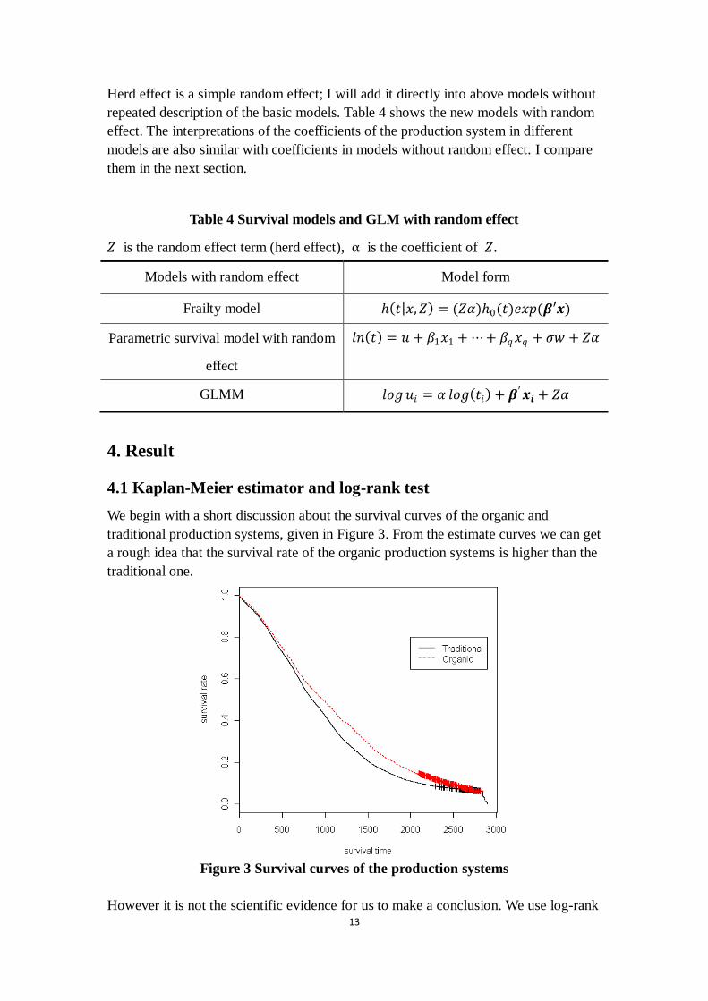
We begin with a short discussion about the survival curves of the organic and

traditional production systems, given in Figure 3. From the estimate curves we can get

a rough idea that the survival rate of the organic production systems is higher than the

traditional one.

Figure 3 Survival curves of the production systems

However it is not the scientific evidence for us to make a conclusion. We use log-rank

14

test to examine whether the difference between traditional and organic production

systems is significant. The result is given in Table 5, where a significant value 10% is

used. The p-value is small enough to reject the null hypothesis (1). The survival rates

of the different production systems are statistically significant.

Table 5 Result of log-rank test

Strata Chi-Square Statistic P-value

System 65.3 6.66e-16

4.2 Cox proportional hazard model and frailty model

Based on the methodology in section 3.1.1.3 and 3.3, the estimation of the Cox

proportional hazard model (denoted as model 1) and frailty model (denoted as model

2) are listed in Table 6.

Table 6 Estimation results of Cox proportional hazard model and frailty model

model 1 model 2

Variable exp(coef) p-value exp(coef) p-value

System 0.9440 <2e-16 0.940 0.000014

calvyr:1999 1.112 <2e-16 1.101 0.0

age 1.0000 0.008610 1.000 0.0

calvmo:2 1.012 0.444636 1.031 0.054

calvmo:3 1.013 0.422877 1.023 0.20

calvmo:4 1.049 0.008958 1.075 0.00018

calvmo:5 1.071 0.000211 1.076 0.00020

calvmo:6 1.060 0.001324 1.066 0.00084

calvmo:7 1.030 0.054136 1.015 0.35

calvmo:8 0.9925 0.576333 0.993 0.61

calvmo:9 0.9623 0.005180 0.958 0.0025

calvmo:10 0.9930 0.616514 0.999 0.93

calvmo:11 1.022 0.1432270 1.019 0.21

calvmo:12 1.041 0.005472 1.045 0.0036

herd -------------- ------------ --------------- 0.0

Clearly in both of the models, the effect of production system is significant. In the

Cox proportional hazard model the relative risk, RR=0.9440<1, means the hazard of

organic production system is less than the traditional production system. In the frailty

model the relative risk, RR=0.940<1, also means hazard of organic production system

is less than the traditional production system. And the effect of herd is significant, test

through the p-value.

15

As shown in the methodology part when relative risk equals to 1, traditional and

organic production systems have the same hazard rate. After adding the random effect

(herd effect) the relative risk is declined, relative risk of Cox proportional hazard

model has a longer distance to 1 than relative risk of frailty model. It means the

influence of the production system to the survival times is strengthened after adding

the random effect.

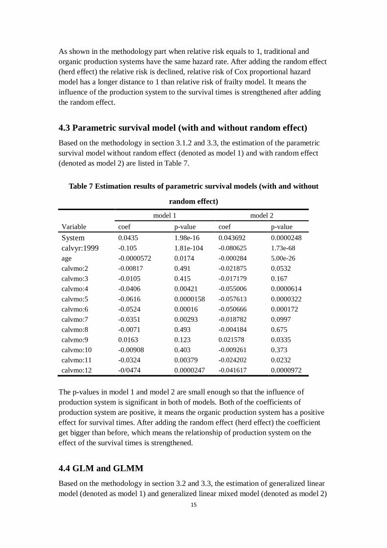
4.3 Parametric survival model (with and without random effect)

Based on the methodology in section 3.1.2 and 3.3, the estimation of the parametric

survival model without random effect (denoted as model 1) and with random effect

(denoted as model 2) are listed in Table 7.

Table 7 Estimation results of parametric survival models (with and without

random effect)

model 1 model 2

Variable coef p-value coef p-value

System 0.0435 1.98e-16 0.043692 0.0000248

calvyr:1999 -0.105 1.81e-104 -0.080625 1.73e-68

age -0.0000572 0.0174 -0.000284 5.00e-26

calvmo:2 -0.00817 0.491 -0.021875 0.0532

calvmo:3 -0.0105 0.415 -0.017179 0.167

calvmo:4 -0.0406 0.00421 -0.055006 0.0000614

calvmo:5 -0.0616 0.0000158 -0.057613 0.0000322

calvmo:6 -0.0524 0.00016 -0.050666 0.000172

calvmo:7 -0.0351 0.00293 -0.018782 0.0997

calvmo:8 -0.0071 0.493 -0.004184 0.675

calvmo:9 0.0163 0.123 0.021578 0.0335

calvmo:10 -0.00908 0.403 -0.009261 0.373

calvmo:11 -0.0324 0.00379 -0.024202 0.0232

calvmo:12 -0/0474 0.0000247 -0.041617 0.0000972

The p-values in model 1 and model 2 are small enough so that the influence of

production system is significant in both of models. Both of the coefficients of

production system are positive, it means the organic production system has a positive

effect for survival times. After adding the random effect (herd effect) the coefficient

get bigger than before, which means the relationship of production system on the

effect of the survival times is strengthened.

4.4 GLM and GLMM

Based on the methodology in section 3.2 and 3.3, the estimation of generalized linear

model (denoted as model 1) and generalized linear mixed model (denoted as model 2)

16

are listed in Table 8.

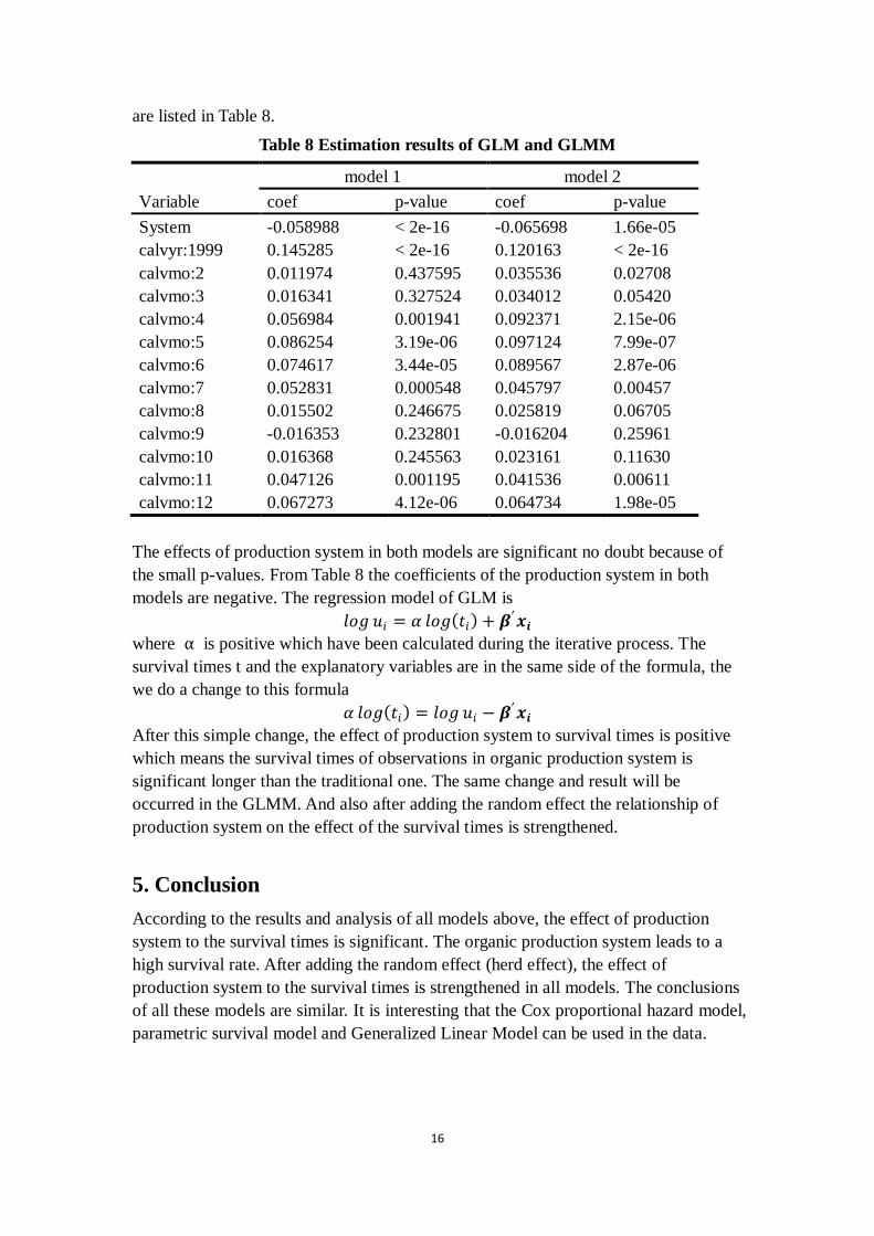
Table 8 Estimation results of GLM and GLMM

model 1 model 2

Variable coef p-value coef p-value

System -0.058988 < 2e-16 -0.065698 1.66e-05

calvyr:1999 0.145285 < 2e-16 0.120163 < 2e-16

calvmo:2 0.011974 0.437595 0.035536 0.02708

calvmo:3 0.016341 0.327524 0.034012 0.05420

calvmo:4 0.056984 0.001941 0.092371 2.15e-06

calvmo:5 0.086254 3.19e-06 0.097124 7.99e-07

calvmo:6 0.074617 3.44e-05 0.089567 2.87e-06

calvmo:7 0.052831 0.000548 0.045797 0.00457

calvmo:8 0.015502 0.246675 0.025819 0.06705

calvmo:9 -0.016353 0.232801 -0.016204 0.25961

calvmo:10 0.016368 0.245563 0.023161 0.11630

calvmo:11 0.047126 0.001195 0.041536 0.00611

calvmo:12 0.067273 4.12e-06 0.064734 1.98e-05

The effects of production system in both models are significant no doubt because of

the small p-values. From Table 8 the coefficients of the production system in both

models are negative. The regression model of GLM is

𝑙𝑜𝑔 𝑢𝑖 = 𝛼 𝑙𝑜𝑔 𝑡𝑖 + 𝜷′𝒙𝒊

where α is positive which have been calculated during the iterative process. The

survival times t and the explanatory variables are in the same side of the formula, the

we do a change to this formula

𝛼 𝑙𝑜𝑔 𝑡𝑖 = 𝑙𝑜𝑔 𝑢𝑖 − 𝜷′𝒙𝒊

After this simple change, the effect of production system to survival times is positive

which means the survival times of observations in organic production system is

significant longer than the traditional one. The same change and result will be

occurred in the GLMM. And also after adding the random effect the relationship of

production system on the effect of the survival times is strengthened.

5. Conclusion

According to the results and analysis of all models above, the effect of production

system to the survival times is significant. The organic production system leads to a

high survival rate. After adding the random effect (herd effect), the effect of

production system to the survival times is strengthened in all models. The conclusions

of all these models are similar. It is interesting that the Cox proportional hazard model,

parametric survival model and Generalized Linear Model can be used in the data.

17

6. Discussion

In this article we only consider the herd effect as a random effect. As we referred in

the introduction section, high genetic relationship exists among dairy cows. If adding

the genetic relationship of cows as the other random effect in above models, it will be

more scientific than only with herd effect. Adding individual effect as a random effect

needs complex technique, we will make a short introduction of the methodology

shown by Yudi Pawitan (Pawitan, 2001).

The process of adding genetic relationship as a random effect is similar as adding herd

effect. The most difficult part is making the relationship matrix which we denote it as

𝑅 here. 𝑅 is a 𝑛 × 𝑛 matrix where 𝑛 is the total number of individuals included in

the dataset we apply in this article. There is a specific dataset providing the basic

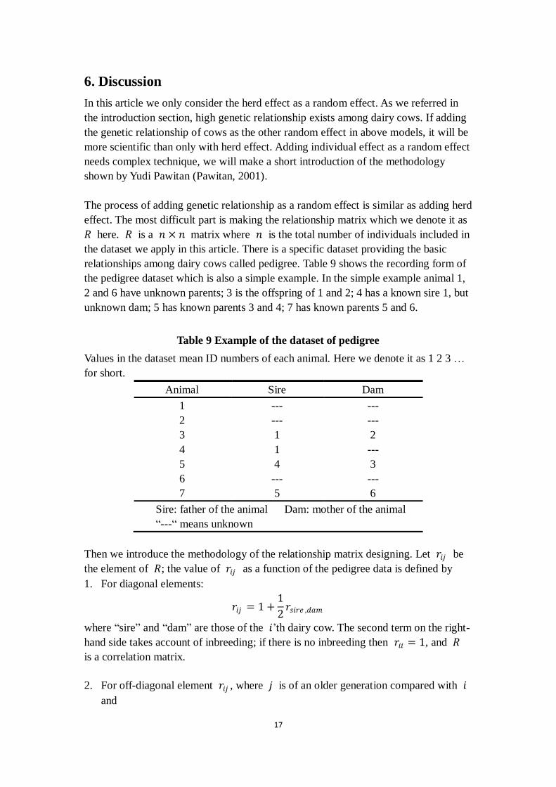
relationships among dairy cows called pedigree. Table 9 shows the recording form of

the pedigree dataset which is also a simple example. In the simple example animal 1,

2 and 6 have unknown parents; 3 is the offspring of 1 and 2; 4 has a known sire 1, but

unknown dam; 5 has known parents 3 and 4; 7 has known parents 5 and 6.

Table 9 Example of the dataset of pedigree

Values in the dataset mean ID numbers of each animal. Here we denote it as 1 2 3 …

for short.

Animal Sire Dam

1 --- ---

2 --- ---

3 1 2

4 1 ---

5 4 3

6 --- ---

7 5 6

Sire: father of the animal Dam: mother of the animal

“---“ means unknown

Then we introduce the methodology of the relationship matrix designing. Let 𝑟𝑖𝑗 be

the element of 𝑅; the value of 𝑟𝑖𝑗 as a function of the pedigree data is defined by

1. For diagonal elements:

𝑟𝑖𝑗 = 1 +1

2𝑟𝑠𝑖𝑟𝑒 ,𝑑𝑎𝑚

where “sire” and “dam” are those of the 𝑖’th dairy cow. The second term on the right-

hand side takes account of inbreeding; if there is no inbreeding then 𝑟𝑖𝑖 = 1, and 𝑅

is a correlation matrix.

2. For off-diagonal element 𝑟𝑖𝑗 , where 𝑗 is of an older generation compared with 𝑖

and

18

(1) both parents of 𝑖 are known

𝑟𝑖𝑗 =1

2(𝑟𝑗 ,𝑠𝑖𝑟𝑒 + 𝑟𝑗 ,𝑑𝑎𝑚 )

(2) only one parent of 𝑖 is known

𝑟𝑖𝑗 =1

2𝑟𝑗 ,𝑠𝑖𝑟𝑒

or

𝑟𝑖𝑗 =1

2𝑟𝑗 ,𝑑𝑎𝑚

(3) both parents of 𝑖 are unknown

𝑟𝑖𝑗 = 0

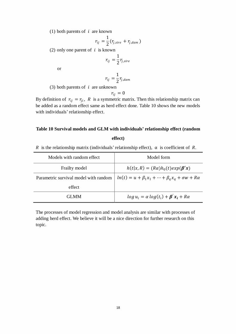
By definition of 𝑟𝑖𝑗 = 𝑟𝑗𝑖 , 𝑅 is a symmetric matrix. Then this relationship matrix can

be added as a random effect same as herd effect done. Table 10 shows the new models

with individuals’ relationship effect.

Table 10 Survival models and GLM with individuals’ relationship effect (random

effect)

𝑅 is the relationship matrix (individuals’ relationship effect), α is coefficient of 𝑅.

Models with random effect Model form

Frailty model 𝑕 𝑡 𝑥,𝑅 = (𝑅𝛼)𝑕0(𝑡)𝑒𝑥𝑝(𝜷′𝒙)

Parametric survival model with random

effect

𝑙𝑛 𝑡 = 𝑢 + 𝛽1𝑥1 + ⋯+ 𝛽𝑞𝑥𝑞 + 𝜎𝑤 + 𝑅𝛼

GLMM 𝑙𝑜𝑔 𝑢𝑖 = 𝛼 𝑙𝑜𝑔 𝑡𝑖 + 𝜷′𝒙𝒊 + 𝑅𝛼

The processes of model regression and model analysis are similar with processes of

adding herd effect. We believe it will be a nice direction for further research on this

topic.

19

Reference

[1] Bewick V., Cheek L. & Ball S., (2004). Statistics review 12: Survival analysis,

Crit Care, v.8(5):389-394.

[2] Miller, R.G., (1981). Survival Analysis, Wiley, New York.

[3] Fahrmeir, L. & Tutz, G.T., (2001). Multivariate Statistical Modelling Based on

Generalized Linear Models, 2nd Edition, Springer-Verlag, New York.

[4] Cox and Oakes, (1984). Analysis of Survival Data, Chapman and Hall

[5] Rodriguez G., (2005). Parametric Survival Models,

http://data.princeton.edu/pop509a/ParametricSurvival.pdf

[6] Everitt B.S. & Hothorn T., (2006). A handbook of Statistical Analyses using R,

Chapman & Hall/CRC, 146-148

[7] Kaplan, E.L. & Meier, P, (1958). ”Nonparametric estimation from incomplete

observations”, Journal of the American Statistical Association 53: 457–481

[8] Peto R. & Peto J., (1972). “Asymptotically Efficient Rand Invariant Test

Procedures”, Journal of the Royal Statistical Society. Series A (General) 135 (2):

185–207

[9] Iachine I., (2001). Basic Survival Analysis,

http://www.biostat.sdu.dk/courses/e02/basalebegreber/bb_sur_e01sm.pdf

[10] Aitkin M. & Clayton D., (1979). The Fitting of Exponential, Weibull and

Extreme Value Distributions to Complex Censored Survival Data Using GLIM,

Applied Statistics, Vol. 29, No. 2 (1980), pp. 156-163.

[11] Pawitan Y., (2001). In All Likelihood: Statistical Modelling and Inference Using

Likelihood, Oxford University Press, USA

20

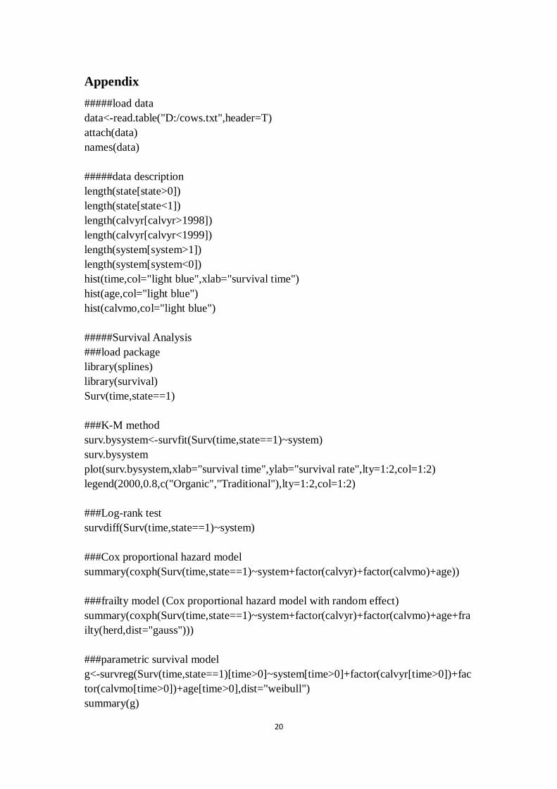
Appendix

#####load data

data<-read.table("D:/cows.txt",header=T)

attach(data)

names(data)

#####data description

length(state[state>0])

length(state[state<1])

length(calvyr[calvyr>1998])

length(calvyr[calvyr<1999])

length(system[system>1])

length(system[system<0])

hist(time,col="light blue",xlab="survival time")

hist(age,col="light blue")

hist(calvmo,col="light blue")

#####Survival Analysis

###load package

library(splines)

library(survival)

Surv(time,state==1)

###K-M method

surv.bysystem<-survfit(Surv(time,state==1)~system)

surv.bysystem

plot(surv.bysystem,xlab="survival time",ylab="survival rate",lty=1:2,col=1:2)

legend(2000,0.8,c("Organic","Traditional"),lty=1:2,col=1:2)

###Log-rank test

survdiff(Surv(time,state==1)~system)

###Cox proportional hazard model

summary(coxph(Surv(time,state==1)~system+factor(calvyr)+factor(calvmo)+age))

###frailty model (Cox proportional hazard model with random effect)

summary(coxph(Surv(time,state==1)~system+factor(calvyr)+factor(calvmo)+age+fra

ilty(herd,dist="gauss")))

###parametric survival model

g<-survreg(Surv(time,state==1)[time>0]~system[time>0]+factor(calvyr[time>0])+fac

tor(calvmo[time>0])+age[time>0],dist="weibull")

summary(g)

21

### parametric survival model with random effect

g1<-survreg(Surv(time,state==1)[time>0]~system[time>0]+factor(calvyr[time>0])+fa

ctor(calvmo[time>0])+age[time>0]+frailty(herd[time>0],dist="gauss"),dist="weibull"

)

summary(g1)

#####Generalized linear model

###GLM

a<-1

for(j in 1:20){

alpha.logt<-a*log(time[time>0])

g<-glm(state[time>0]~system[time>0]+factor(calvyr[time>0])+factor(calvmo[time>0

])+age[time>0]),family=poisson(link=log),offset=alpha.logt,data=data)

u.hat<-g$fitted.values

alpha.hat<-((sum((u.hat-state[time>0])*log(time[time>0])))/length(time[time>0]))^(-1

)

alpha.new<-(alpha.hat+a)/2

a.old<-a

a<-alpha.new

}

print(abs(alpha.new-a.old))

print(summary(g))

#GLMM (GLM with random effect)

library(Matrix)

library(lattice)

library(lme4)

a<-1

for(j in 1:20){

alpha.logt<-a*log(time[time>0])

g1<-lmer(state[time>0]~system[time>0]+factor(calvyr[time>0])+factor(calvmo[time

>0])+age[time>0]+(1|herd[time>0]),family=poisson(link=log),offset=alpha.logt,data=

data1)

u.hat<-fitted(g1)

alpha.hat<-((sum((u.hat-state[time>0])*log(time[time>0])))/length(time[time>0]))^(-1

)

alpha.new<-(alpha.hat+a)/2

a.old<-a

a<-alpha.new

}

print(abs(alpha.new-a.old))

print(summary(g1))