水路部研究報告第32号平成8年3月27日

REPORT OF HYDROGRAPHIC RESEARCHES N o.32 March, 1996

Interpolation of Bathymetric data using two-dimensional OFT

approximate expression↑

Akira ASADA *

Hydrographic Department of Japan t

Abstract

For establishment of the more advanced interpolation method of bathymetric mesh data, the

interpolation method using two-dimensional Discreet Fourier Transform approximation of 32* 32

or 64 * 64 mesh data has been studied. This interpolation method has high capabilities of topograph-

ical approximation. Since it is able to grasp the lineament and features of complicated topography

well using many coefficients, it has high ability of the interpolation. The basic process to obtain

two-dimensional Discreet Fourier Transform approximation is the repeated calculation of each

frequency components by least squares method. Especially, it is important to repeatedly calculate

the small frequency components which have longer wave length than the area of deficit part. The

calculation order among directional components of same frequency follows their approximate

values. In according to the deficit condition of bathymetric mesh data, frequency components of

calculation are selected in advance. For the area of large deficit part, trial results of this method

were satisfied.

1. Introduction

Several problems exist when a seafloor topo-

graphical map is prepared from multi-beam

data. We must solve these problems. One of

them is interpolation of deficit parts. The

approximate interpolation program using lin-

ear, quadratic, and cubic polynomial expres-

sions has been established and has been used

until now (Asada et al, 1989). As a result, a

good result was obtained in the case of small

blank area. However, there were various prob-

lems for interpolation of large deficit parts of

data. In a large deficit part case, it is possible

to create undesirable artificial topography.

However, personnel in correction of the com-

puter drawing contour chart could not always

t Received 1996 February !st Accept巴d1996 Mar℃h 7th ＊海洋研究所 OceanRes巴archLaboratory

49

notice the undesirable artificial topography.

In order to solve large deficit part case, the

author paid attention to two悶dimensionalDis-

creet Fourier Transfer (DFT), one of the tech-

niques used to analyze seafloor topography. He

studied the two-dimensional DFT approxima-

tion expression that can effectively process

features of seafloor topography, and completed

a practical interpolating method using that

express10n.

2. The cubic polynomial approximate

interpolation

One purpose for this study is aimed at

advanced interpolation method of seafloor top-

ographical data. The cubic polynomial approx-

imation method of X -Y with 16 coefficients has

AkirαASAD A

The whole sampling block cannot be approx-been used up to now.

imated well in this case. Since the topography Z= :LJ. 2J (amnキxm*yn)

m=On=O of a cliff, valley, and fault cannot be approx”

(1)

and roughly approxi立1atesit well, imated In the case of small deficit parts, they can be

requires a matching process with the real data. cubic the usmg successfully interpolated

For the flat region under a cliff, a fine flat a Fig.1, In above. express10n polynomial

plane is naturally created by sediment in the sounding chart (3) shows the distribution of

large a of the cliff. If, however, extension mesh depth data with blank rows equivalent to

deficit part of data exists around these places, about 5 times as a mesh size. In case of this

artificial topography such as landslip, hole, and scale deficit parts, the interpolation using the

knoll were frequently created by the interpola輔plane approximation gave us a unsatisfactory

ti on (see Fig. 3 ) . Editing personnel could not we could get a satisfactory But, result (2).

always notice incorrect portions of the inter-contour chart (1) by the interpolation using the

polated seafloor topography map. Fig. 2 shows cubic polynomial approximation. Only in case

this example of contour chart with undesirable of interpolation using the cubic polynomial

artificial topography. problems for larger approximation, various

In the conventional processing system, the deficit parts of data occur. In a large deficit

topography map is interpolated using a com同part case, the sampling size must be expanded

region has been each defective and puter, However, the for the interpolation process.

manually modified by the engineer. Therefore, features of large制scaletopography cannot be

it is necessary to establish the more advanced approximate an usmg correctly grasped

interpolation method and a program not depen” expression only with 16 coefficients. The prob-

dent upon modification by the editors. lem of divergence occurs also when the order

of polynomial expression increases.

一主長及、民主主公きどきさ刊誌由唱え抗議法定要Mwr

す次官坊主

ssug－－、宮廷寄託事室抽選議砂漠hv－

込事長川

1335災時きおい認さ設詳謀長検議選－

一弘冷前日主主主主awvd己建設さ話器護法議、、

主主主主若者毛沢」J

ミミ明言町襲撃泊予

3判明

His史上霊童話霊童喜一撃

さまS主主売をもミh茎をもか

h

零註悪柏市＆S事

主主

E5353F5意義峯選察、

(1) contour interval 20m (2) contour interval lOm (3) sounding chart

Fig. 1 Mesh data interpolation using the cubic polynomial approximation

(1) Result of satisfactory interpolation using the cubic polynomial approximation

(2) Result of unsatisfactory interpolation using the plane approximation

(3) Distribution of mesh depth data with blank rows equivalent to about 5 times as a mesh size

50

Interpolαtion of Bαthy metric dαtα using two・dimensionalDFTα.pproximαte expression

ノ

Fig. 2 Contour chart with undesirable artificial topography (marked with .C:.) was processed by the cubic

polynomial approximate interpolation

Fig. 3 Three-dimensional seafloor image map around Okusiri Island with undesired artificial

topography with arrowheads that was processed by the cubic polynomial approximate interpo-

la ti on

51

AkirαA SADA

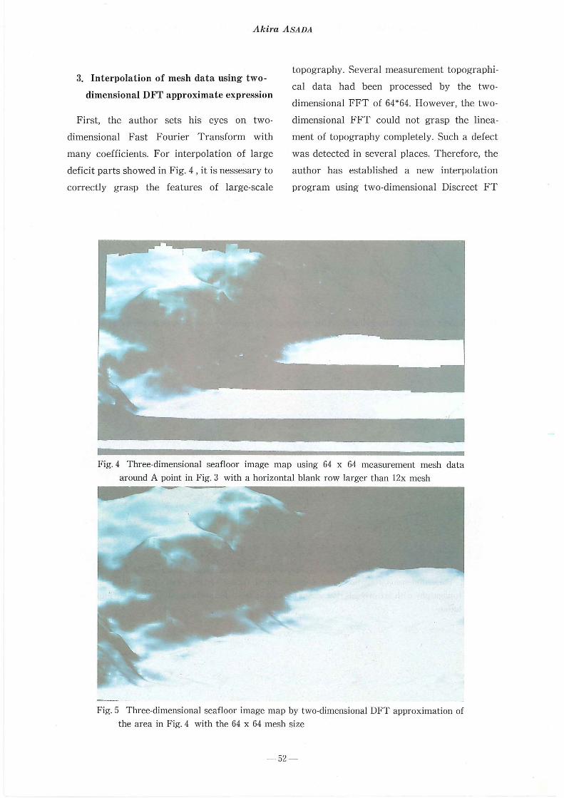
3. Interpolation of mesh data using two-

dimensional DFT approximate expression

First, the author sets his eyes on two-

dimensional Fast Fourier Transform with

many coefficients. For interpolation of large

deficit parts showed in Fig. 4 , it is nessesary to

correctly grasp the features of large-scale

topography. Several measurement topographi-

cal data had been processed by the two-

dimensional FFT of 64*64. However, the two司

dimensional FFT could not grasp the linea-

ment of topography completely. Such a defect

was detected in several places. Therefore, the

author has established a new interpolation

program using two-dimensional Discreet FT

Fig. 4 Three-dimensional seafloor image map using 64 x 64 measurement mesh data

around A point in Fig. 3 with a horizontal blank row larger than 12x mesh ‘司．． ，，一ーー－

Fig. 5 Three-dimensional seafloor image map by two-dimensional DFT approximation of

the area in Fig. 4 with the 64 x 64 mesh size

- 52-

Interpolαtion of Bαthy metric dαta using two-dimensionαl DFTα:pproximαte expression

approximate method that compensates for this

defect. The interpolation using the two喝

dimensional DFT approximation give us a

satisfactory result in Fig. 5 .

The two-dimensional DFT is given by the

following expression.

Z’二~ ~ {amn* cos(CoJrnX +wnY) + m=On=-32

bmn * sin ( WmX十WnY)} (2)

To grasp the lineament and features of com”

plicated topography well, each component of

(WrnX十wnY) is calculated in the order of

increasing frequency and catching precise char-

acteristics of topography. At each step, the

component value is subtracted. The叫ncon-

tains only a positive region, and the wn not only

a positive component but also a negative

reg10n.

In this approximate method, each frequency

component is piled up with deficit parts of

data. In other words, some characteristics of

topographies with different liniations are piled

up. To approximate to sample data, approxi-

mate calculation is performed irrespective of

the blank area in data. Therefore, the maxi-

mum amplitude of real data is monitored in the

process of approximation. The data with a

frequency component higher than the maxi-

mum amplitude of real data in this stage is

eliminated as an error.

The reference frequency with wavelength of

about 1.5 to 2 times as high as the maximum

sampling size of mesh data, is selected so that

each frequency is the integer multiple of its

reference frequency. As a result, the whole

topography of the mesh data could be approx”

imated better. The parameter for this wave-

length is used to correspond to the mesh size

and the topography scale of the area.

Sequential calculation from a low frequency

53

component is recommended. Moreover, the

topography can be grasped well by repeating

the approximate calculations of low frequency

components. The greatest problem of the two-

dimensional DFT is that a frequency compo”

nent in an X -Y direction can be also approx-

imated using the other frequency component

with different or same wavelength in other X

-Y direction. In other words, a program must

be designed so that it is best matched for the

seafloor topography.

An unnatural approximation occurs in the

deficit parts of data due to the relation between

the deficit distribution status of data and the

direction of a frequency component. Therefore,

a filtering function was added for the fre-

quency component in the direction easily in”

fluenced by deficit distribution of data, and is

not calculated.

In the cubic polynomial approximate expres-

sion of X Y, the Z value significantly diverges

when position is far from (0, 0). However,

there is no divergence in the two-dimensional

DFT. The number of coefficients basically

becomes 4096 (32*64 *2) and can grasp the

topography accurately. However, considerable

calculation time is required. It takes five min-

utes to obtain a satisfactorily approximate

expression of 64句4using the program in the

current stage. A work station of arithmetic

speed lOOMIPs is used in this case. Since some

ten thousands of interpolation points must be

calculated practically, in the current stage, the

approximate size is prescribed as units of 32*32

due to limitation in the arithmetic operation

speed of a computer. It is necessary to use the

units of 64 *64 if the deficit region becomes very

large.

The interpolation capability was improved

by limiting each frequency component calcu-

AkirαASAD A

lated according to the data deficit status.

Filtering was designed before approximate

calculation. For an example given in Fig. 7, the

frequency component in the X direction is lim-

ited in a range 0 to 12 times as high as the

reference least frequency. The frequency com-

ponent in the Y direction is limited in a range

0 to 3 times as high. In this case, a interpolation

result was highly improved. About ten days

were required for calculation to interpolate all

the deficit regions in Fig. 7. The result using

the two-dimensional DFT approximation in

Fig. 7 was improved more so than unsatisfac-

tory result of the approximate methods using

the cubic polynomial expression of X -Y in Fig.

6.

4. How to obtain two-dimensional DFT

approximate expression

(Basic expression and it’s definition)

Fig. 6 Unsatisfactory three dimensional seafloor image off Akita by linear-cubic polynomial

approximate interpolation in the 520 x 460 mesh size. It took about 10 minutes to complete

processmg.

Fig. 7 Improved three-dimensional seafloor image off Akita by two-dimensional DFT approximate,

interpolation in the 520 x 460 mesh size. It took about seven days to complete processing.

54

Interpolation of Bαthymetric dαtα using two-dimensionαl DFTα:pproximαte expression

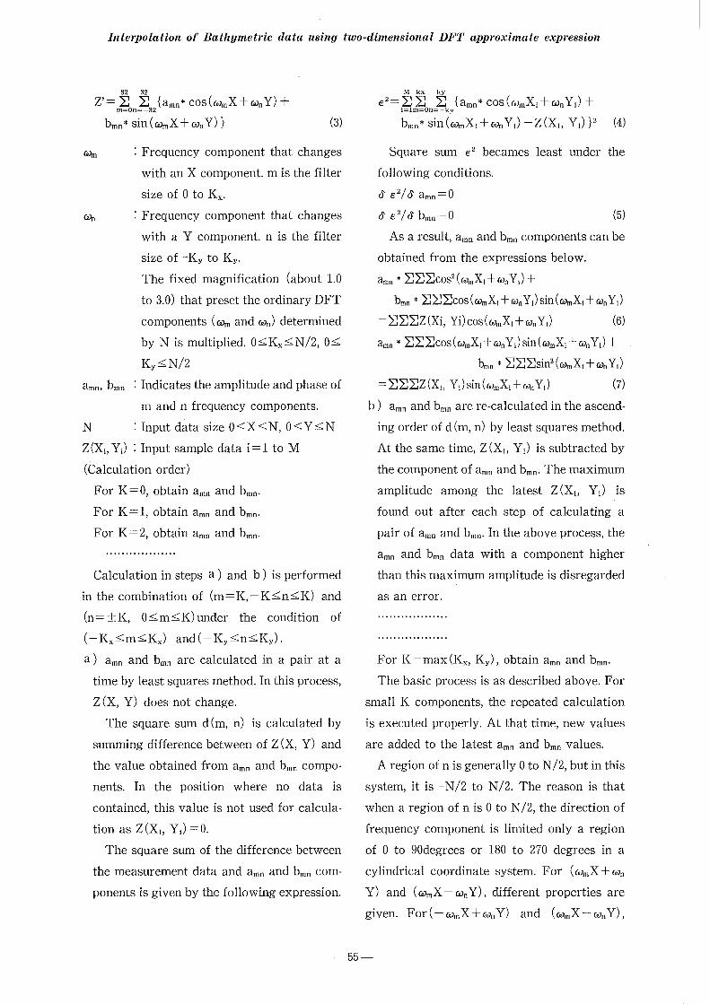
z’＝ ~On~az { amn * COS （均X+wnY）十

bmn~ (3)

Wm

Wn

amn,

: Frequency component that changes

with an X component. m is the filter

size of 0 to Kx・

: Frequency component that changes

with a Y component. n is the filter

size of -KY to Ky.

The fixed magnification (about 1.0

to 3.0) that preset the ordinary DFT

components (Wm and wn) determined

by N is multiplied. O 三三 Kx~二N/2, 。三二

Ky三二N/2

m and n frequency components.

N : Input data size O三二XζN,O三二YζN

Z (Xi, Y1) : Input sample data i = 1 to M

(Calculation order)

For K=O, obtain amn and bmn・

For K = 1, obtain amn and bmn・

For kニ 2,obtain amn and bmn・

Calculation in steps a) and b) is performed

in the combination of (m = K, -Kζn~二K) and

(nニ土K, O三二m三二K)under the condition of

( Kx三二m三二Kx) and(-Ky三三n三二Ky).

a) amn and bmn are calculated in a pair at a

time by least squares method. In this process,

Z (X, Y) does not change.

The square sum d (m, n) is calculated by

summing difference between of Z (X, Y) and

the value obtained from amn and bmn compo-

nents. In the position where no data is

contained, this value is not used for calcula-

tion as Z (Xi, Y1) = 0.

The square sum of the difference between

the measurement data and amn and bmn com-

ponents is given by the following expression.

-55

M kx ky e2 ＝呂l1加＝~ky{amn* cos(WrnX1+w品）＋

bmn*

Square sum e2 becames least under the

following conditions.

6ε2/ o amn=O δε2/ 0 bmn =O (5)

As a result, amn and bmn components can be

obtained from the expressions below.

amn * 2J2J2Jcos2(WmX1+wnY1）十

bmn * 2J 2J LJcos （白石nX1十wnY1)sin（均X1十WnY1)

=LJLJLJZ(Xi, Yi)cos（均X1十WnY1) (6)

amn * 2J2J2Jcos(WmX1十WnY1) sin (WroX1十wnY1)+

bmn * 2J2J2Jsin2 (WmX1 + wnY1)

=2J2J2JZ(Xi, Y1)sin(WmX1+wnY1) (7)

b) amn and bmn are re-calculated in the ascend-

ing order of d (m, n) by least squares method.

At the same time, Z (Xi, Y1) is subtracted by

the component of amn and bmn・ The maximum

amplitude among the latest Z (X1, Y1) is

found out after each step of calculating a

pair of amn and bmn・Inthe above process, the

amn and bmn data with a component higher

than this maximum amplitude is disregarded

as an error.

For K=max(Kx, Ky), obtain amn and bmn・

The basic process is as described above. For

small K components, the repeated calculation

is executed properly. At that time, new values

are added to the latest amn and bmn values.

A region of n is generally 0 to N/2, but in this

system, it is -N/2 to N/2. The reason is that

when a region of n is 0 to N /2, the direction of

frequency component is limited only a region

of 0 to 90degrees or 180 to 270 degrees in a

cylindrical coordinate system. For （向X+wn

Y) and (c.JrnX wn Y), different properties are

given. For ( WrnX十wnY) and （叫nX-wnY),

AkirαASAD A

the signs of amn and bmn are only inverted, and

the same topographical property is obtained.

At last, approximated Z’（X, Y) is obtained

by inversion of two-dimensional DFT from

determined amn and bmn・Foronly the center

value of approximate Z’（X, Y), the approxi-

mate value is directly used. In this case, the

center position of Z’（X, Y) is matched to the

interpolation point. In another case, the center

value is modified by the matched process

between Z’（X, Y) in inverse proportion of

square distance from the interpolation point.

5, Conclusion

Interpolation using the two-dimensional

DFT approximation requires a large amount of

processing time. However, this interpolation is

expected to be effective in improving the level

of subsequent editing and in obtaining high

quality results. How to determine the parame-

ters corresponding to seafloor topography, and

how to approximate with excellence, must be

continuously studied in future.

The two-dimensional DFT approximation

method is able to be directly used for the fre-

quency analysis of seafloor topography. Other

applications being considered include the tex”

ture analysis of topography, the elimination of

noise in topography, the metamorphism of

topography, and the analysis of activities. This

method covers for the faults in two-

dimensional FFT. Therefore, it enables an

advanced analysis.

The author thanks Professor Asahiko Taira

of Ocean Research Institute, Tokyo University

and Professor Tomoyoshi Takeuchi of the

University of Electronic-Communication for

their valuable instructions and advice provided

for the author in preparing this paper.

-56

Reference

A. Asada : 3 D image processing of Sea Beam

bathymetric data-as applied from the

Sagami trough to the Izu・Ogasawara

trench, Reρart of Hydrographic

Researches, 21, 113-133, (1986).

A. Asada and A. Nakanishi : Contour process-

ing of Sea Beam bathymetric data,

Reρart of局1drographicResearches, 21,

89-110, (1986).

A. Asada and S. Kato and S. Kasuga :

Tectonic landform and geological struc-

ture survey in the Toyama Trough,

Report of JかdrograρhieResearches, 25,

93 122, (1989).

2次元 DFT近似式を使った海底地形データの補

間法（要旨）

浅田昭

海底地形データ処理過程において、海底の地形

の特徴を上手く捉えた優れた水深メッシュデータ

の補間法の確立が望まれている。このため、 64×

64または32×32個の 2次元DFT近似式を使った

補関処理法の研究を行い、かなり満足のいく補間

法を作成した。 2次元DFT近似式は非常に沢山

の係数を持っており、複雑な海底地形を表すこと

や、地形のリニアメント等の特徴を捉えるができ

る。それ故、高い補間能力を持っている。基本的

な2次元DFT近似式の求め方としては、地形の

特徴をうまくとらえることが重要で、ある。地形

データから最小白：乗法を使い、繰り返し計算によ

り最良の各周波数成分の近似値に近づける方法を

取った。得に、テータの欠損部の大ききよりも長

い波長を持つ低周波領域において、最初に、入念

な繰り返し計算により近似値を求めることが肝心

である。最大波長も DFT計算データ領域より 1.5

倍程度大きくすると良い結果が得られる。また、

計算順序についても、低周波成分の方から処理し、

同じ周波数でも成分の近似値の大きい方向のもの

Interpolαtion of Bαthymetric dαtα using tw小 dimensionαlDFTα：pproximαte expression

から順に計算し、その成分値を除去しながら繰り

返し計算を行う等の工夫を施した。データの欠損

状況に応じて、求める周波数成分を予め制践する

フィルター機能も付加した。こうして得られた 2

次元DFT近似式を使って、かなり大きなテータ

の欠損部を持つテ、、ータについて良い補間結果が得

られた。

57