INTERNSHIP REPORT

NUMERICAL MODELING OF SPLAY FAULT IN A SUBDUCTION ZONE

School of Engineering and Applied Sciences of the Harvard University

Advisors: James R. Rice and Renata Dmowska

Stéphanie Raoul Summer 2007

SUMMARY

I. Model descriptions…………………………………………………………….….……..1 a. Influence of parameters……………………………..………………….………….2 b. Model configuration……………………………………………………………….3 c. Slip-weakening friction law……………………………………………………….3 d. Choice of parameters……………………………………………………………....4 II. Numerical modeling...……………………………………………………….………....5

a. Input file descriptions………………....…………………………………………...5 b. Mesh descriptions……………………………………………………….………....6

III. Results………………………………………………………………………………....8

a. Meshes ………………………………………………………………...………….8 b. Depth dependent stresses………………………………………………………...10 c. Verification test using case study of Kame et al. (2003)………………………...11

IV. Conclusion…………………………………………………………………………...13

1

Oceanic subduction occurs when the oceanic plate slides under the continental plate. The release of the force due to the slippage can cause violent earthquakes that can be deep along the plate interface or shallow, approaching the seafloor. The subduction zone geometry includes main and branching faults. The comprehension of this zone is very important, first because a many large magnitude earthquakes are located there and second because these earthquakes can generate tsunamis. The tsunamis are caused when the rupture reaches close enough to the surface to cause significant seafloor deformations. The tsunami generated depends on the path chosen by this rupture: i.e., for similar amounts of accommodated slip, if the rupture takes the splay fault, then the seafloor deformation would than had the rupture taken the main fault. The path choice of the rupture propagation between the main or branching fault or the both is controlled by. the splay step-up angles, the depth-dependent stresses, and the material contrast across fault interface (figure 1). Kame et al., (2003) and Bhat et al., (2007) have shown that branch activation during dynamic slip-weakening rupture can have large effect on the rupture propagation along the main fault, and can in some cases stop this propagation. Whether rupture propagation occurs along the main fault, along the branch or along both depends principally on the prestress state, the angle between the branch and the main fault, the rupture velocity in the junction of the branch, and whether the branch is to compressional side or extensional side (Poliakov et al., 2002; Kame et al., 2003). During earthquakes in the cases of subduction zone environments, activation of splay faults can occur. Activation of splay faults can have major effects on deformation of the seafloor. The aim of my internship was to do a numerical simulation of splay fault of a subduction zone, in dynamics of Tsunami genesis. The goal of this simulation is to better understand which condition is necessary to activate a splay fault, the effects that it have on the main fault and when the rupture on the main faults is a significant contribution to the moment release. (figure 1)

I. Model descriptions

Some parameters that control the propagation of the rupture along the main and splay fault include: the angle ϕ between the main and the splay fault, the state of stress in the region before the earthquakes nucleates, and the rupture velocity in the junction of the branch and the length of the branch.

2

a. Influence of parameters

Poliakov et al., (2002) and Kame et al., (2003) showed that the inclination of the maximum principal stress in the prestress state, Ψ, can control the path chosen during the dynamic rupture propagation. For a low angle, Ψ ,between the maximum prestress Smax and the main fault, the stresses at the crack tip increase significantly from the prestress on the both sides of the fault. While for a higher Ψ, the high stress (particularly for Ψ>45) is on the extensional side of the main fault. Kame et al. (2003) and Bhat et al. (2004) showed as well that when ψ decrease the favorable branch for the rupture propagation switches to the extensional side from compressional side (figure2)

figure 2

Furthermore this angle controls the path of the rupture propagation. For example, with a rupture velocity fixed at vr=0.6 cs they showed that for an angle Ψ equal to 56, 25, and13, the rupture propagation chose respectively, the extensional branch, the main fault and the compressional branch (figure 3)

Ψ = 56° ϕ = -15° Vr= 0.6 Cs

Ψ = 25° ϕ = -15° Vr= 0.6 Cs

Cd t/Ro is the time after the beginning of the rupture. x/Ro is the distance

Ψ = 13° ϕ = 15° Vr= 0.6 Cs

figure 3

3

Kame et al. (2003) showed that the propagation along the both faults is more difficult for a small angle between the splay and main fault. The rupture velocity is also very important; the path chosen by the rupture propagation depends on it. For example, for an inclination Smax and an angle ϕ fixed Kame et al., 2003 showed that for vr equals to 0.8 Cs , 0.9 Cs the rupture chooses the branch, and for 0.6 Cs it propages along the both, but stops on the branch path very close of the junction (figure 4).

figure 4

They showed as well that when the branching angle ϕ is equal to ±15° and the angle of Smax equal to Ψ=13° for ϕ=15° and Ψ=56°,70° for ϕ=-15°, the rupture stops on the main fault for all velocities except vr=0.9Cs due to the reduced interaction between the main and branched faults. However when Ψ approached 0° or 90° the rupture stop on the main fault for vr=0.9 Cs. Bhat et al. (2004) showed that for a compressional side and a medium velocity the length of the branch affects the rupture propagation on the main fault (Ψ=13° , ϕ=15°, vr=0.8 Cs), and investigated finite branch lengths ranging from 1R0 to 30 R0, where R0 is the size of the static slip-weakening zone. They showed that for extensional side, while the infinite branch allows continuation of rupture on the main fault for high velocity and low branch angle, a finite branch led the continuation on the main fault for (Ψ=70°, Lbr= 6.20Ro) For this same case, they showed that when Lbr= 30R0 the terminating rupture close to the main fault led to re-nucleation of rupture on the main fault.

b. Model configuration We consider slip-weakening dynamic shear rupture propagating along the subduction zone plate interface and encountering a splay fault. The splay fault forms an angle ϕ with the main fault. This fault system is embedded in an isotropic elastic material. We consider two fault system geometries: A deep section the system in an infinite environment and a shallow section where the effects of the seafloor surface are considered. . The slip is tangential to the fault. The prestresses in the medium are

Ψ = 13°

4

horizontal

!

"#xx

0( ) and vertical

!

"# yy

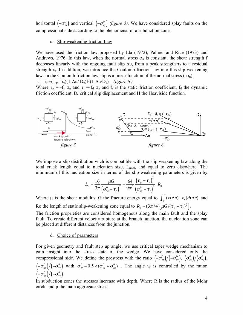
0( ) (figure 5). We have considered splay faults on the compressional side according to the phenomenal of a subduction zone.

c. Slip-weakening friction Law We have used the friction law proposed by Ida (1972), Palmer and Rice (1973) and Andrews, 1976. In this law, when the normal stress σn is constant, the shear strength f decreases linearly with the ongoing fault slip Δu, from a peak strength τp to a residual strength τr. In addition, we introduce the Coulomb friction law into this slip-weakening law. In the Coulomb friction law slip is a linear function of the normal stress (-σn): τ = τr +( τp - τr)(1-Δu/ Dc)H(1-Δu/Dc) (figure 6 ) Where τp = -fs σn and τr =-fd σn and fs is the static friction coefficient, fd the dynamic friction coefficient, Dc critical slip displacement and H the Heaviside function.

figure 5 figure 6 We impose a slip distribution wich is compatible with the slip weakening law along the total crack length equal to nucleation size, Lnucl, and equal to zero elsewhere. The minimum of this nucleation size in terms of the slip-weakening parameters is given by

zzzzzzzzzzzzzzzzzzzzzzz

!

Lc =16

3"

µG

# yx

0$ % r( )

2=64

9" 2

% p $ % r( )2

# yx

0$ % r( )

2R0

Where µ is the shear modulus, G the fracture energy equal to

!

(" (#u) $0

%

& "r)d(#u) and

Ro the length of static slip-weakening zone equal to

!

R0

= (3" /4) µG /(# p $ # r )2[ ] .

The friction proprieties are considered homogenous along the main fault and the splay fault. To create different velocity rupture at the branch junction, the nucleation zone can be placed at different distances from the junction.

d. Choice of parameters

For given geometry and fault step up angle, we use critical taper wedge mechanism to gain insight into the stress state of the wedge. We have considered only the compressional side. We define the prestress with the ratio

!

"# zz

0( ) "# yy

0( ),

!

" xy

0( ) " yy

0( ),

!

"# xx

0( ) "# yy

0( ) with

!

" zz

0= 0.5 # (" yy

0+" xx

0) . The angle ψ is controlled by the ration

!

"# xx

0( ) "# yy

0( ). In subduction zones the stresses increase with depth. Where R is the radius of the Mohr circle and p the main aggregate stress.

5

The slip-weakening law depends on the value of the friction coefficient fs and fd, and on Dc. We defined different values for the splay and main fault. The normalized shear stress along the fault was fixed to set the seismic S ratio

!

S = (" p #$ xy

0) /($ xy

0# " r ). In the case of

S<1.77 supershear rupture is predicted . For good resolution we defined R0= N ΔX with N=20 and ΔX equals to the element length. The material properties are defined according the materials in the subduction zones. The direction of the maximal stress Smax makes angle ψ with the direction of the main fault. β is the angle between the horizontal and the main fault, α is the angle between the horizontal and the surface, ϕ is the angle between the main fault and the branch (figure 7)

figure 7 For a deep section we have used the value α=4°, β=4°, ϕ=23°, we use a low angle ψ. We take the ratio

!

"# xy

0( ) "# yy

0( ) = 2.361. We use the static coefficient for the main fault equals to 0.6 and for the splay fault equals to 0.5. For a shallow section we use the value α=2°, β=1°, ϕ=20°,

!

"# xy

0( ) "# yy

0( ) = 2.361,

!

" xy

0( ) " yy

0( ) = #0.157 and

!

" yy

0= #120.10

6Pa . We use the static friction coefficient for the

main fault equal to 0.6 and for the splay fault equals to 0.35

II. Numerical modeling ABAQUS/Explicit is a commercial program based on the finite elements method. This software needs discretization geometry. The geometry is modeled with nodes, elements and surface. Each element represents a discrete portion of the physical structure. This physical structure is represented by a lot of interconnected elements that are connected to one another by nodes. The input file (.inp) must contain the geometry of the structure, its material behavior, its boundary conditions, the loads applied and the output request.

a. Input file descriptions

Definition of the model geometry ` The geometry is a mesh containing nodes, elements and surfaces. We use plane strain elements of type CPE3. To generate them we used the functions (*NODE, *ELEMENT, *NSET, *ELSET, *ELGEN, *NFILL). We use plane strain infinite elements of type CINPE4. To generate it we used (*NODE, *ELEMENT, *NSET, *ELSET, *ELGEN, *NFILL). Definition of the material properties The comportment law (material’s mass density, material properties, material comportments) is defined with the functions (*MATERIAL, *DENSITY, *ELASTIC, *SOLID SECTION)

6

Definition of the boundary conditions The initial conditions are the prestress applied on the medium .The stress is applied with the function (*INITIAL). Contact definition The main and splay faults are defined like a pairs of node sets and surfaces that make contact. There is a friction property into this contact. This contact is generated by (*SURFACE INTERACTION, *FRICTION, *CONTACT PAIR). To define the friction law, we used an input file where is written in FORTRAN language. Dynamic stress definition There is dynamic stress that defined with the functions (*STEP, *DYNAMIC) Output request To avoid using excessive disk memory, we have limited our request to contact and element’s writing in the database.

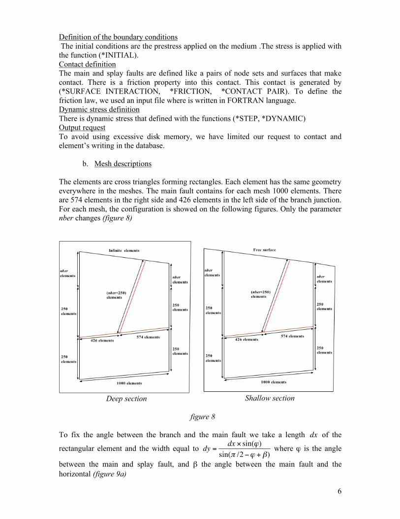
b. Mesh descriptions a)

The elements are cross triangles forming rectangles. Each element has the same geometry everywhere in the meshes. The main fault contains for each mesh 1000 elements. There are 574 elements in the right side and 426 elements in the left side of the branch junction. For each mesh, the configuration is showed on the following figures. Only the parameter nber changes (figure 8)

Deep section

Shallow section

figure 8 To fix the angle between the branch and the main fault we take a length

!

dx of the

rectangular element and the width equal to

!

dy =dx " sin(#)

sin($ /2 %# + &) where ϕ is the angle

between the main and splay fault, and β the angle between the main fault and the horizontal (figure 9a)

7

The angle between the surface and the horizontal is fixed with the difference of the length between the right side and the left side of the top of the mesh. (a)

(b)

figure 9 Where

!

Dl are equal to

!

Dl = Dr + dx " nbe " cos(#) " tan($) with

!

nbe elements number between the node A and B. Because of there are the same number of elements but a different length on the left-side and right-side (figure 9b) , Dr must be approximately equal to

!

Dr " nber # dy $ Nb # dx # cos(%) # (tan(&) + tan(%)) with

!

nber the number of element between the node C and A or D and B and

!

Nb the number of elements on the right-side of the branch (figure 10)

figure 10

The branch and fault are defined with a duplicate set of nodes. The original set of nodes defines the slave surface node. The duplicate set of nodes is used to define the master surface. The junction between the branch and the fault is defined without contact between the master surface of the fault and the master surface of the branch so that there is a tiny jump, on the order of R0/20, between the main fault and the splay fault (figure 11) For the deep section the entire medium is surrounded by infinite elements. For the shallow section the medium is surrounded on the left, right, and bottom by infinite so that in the case of shallow section, the top of the mesh reaches the sea floor.

8

Junction between main and splay fault

Master surfaces MASTERM2 and MASTERB

Master surfaces MASTERM1 and MASTERB

Slave nodes NSLAVE1 and NSLAVEB

Slave nodes NSLAVE2 and NSLAVEB Slave nodes NSLAVE1 figure 11

III. Results

a. Meshes

Subduction zones are very interesting because the deepest earthquakes occur only in these zones, although shallow and medium earthquakes take place as well. The difference between the deep section and shallow section are the geometry (the dip of the fault, the splay step-up angles) and the material contrast. The accretionary prism can be modeled near the surface of the subduction, and it depends of the subduction geometry. To

9

represent this accretionary phenomena it was very important to create for a model whose deep section had less material contrast than the shallow section. *Deep section

Type of elements: The infinite elements are used to simulate an infinite medium. These elements prevent wave reflections generated by the rupture at the boundaries of the model to simulate an infinite domain. The finite elements are use to simulated the medium.

Material contrast: We have modeled a mesh for a deep section with a bimaterial contrast. In this case the materials are separated by the main fault.

*Shallow section Type of elements: In the case of a shallow surface, there are no infinite elements on the top of the mesh. In fact, according to the geometry of a shallow section in the oceanic subduction zones, the seafloor is on the surface.

Infinite elements

Finite elements

20° 4°

4°

MATERIAL B

MATERIAL A

10

Type of materials: We have modeled a mesh for a shallow section, with a bimaterial contrast.

b. Depth dependent stresses

Because of in the subduction zone, there is a depth dependent stresses, we have verified that the For a mesh with branch angle of 25° and a surface angle of 14°.

Infinite elements

Finite elements 23°

1°

2°

MATERIAL C MATERIAL B

MATERIAL A

11

c. Verification test using case study of Kame et al. (2003)

We have done a test with ψ=56° and ϕ=15° at which the rupture encounters the branch at high velocity, in order to verify the dynamic rupture model. We find that the rupture does not take the branch:

Step time = 0.7707

Step time = 1.541

Step time = 3.083

Step time = 5.394

Our results agree with Kame et al:

12

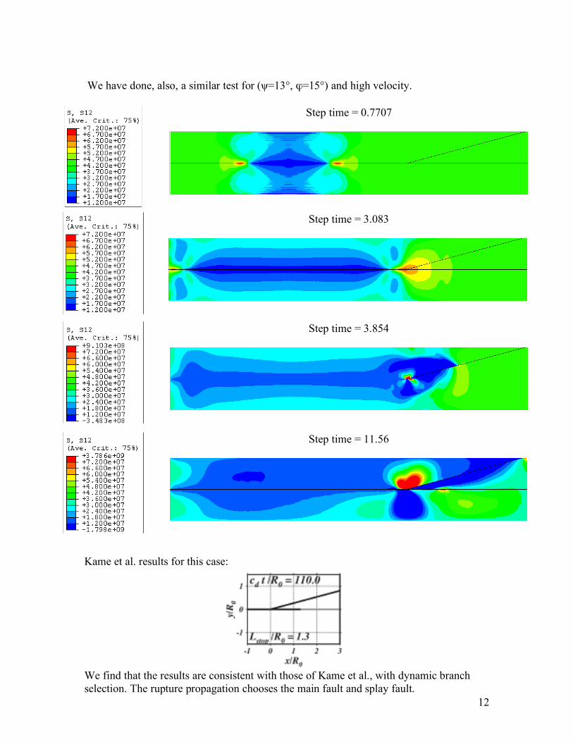
We have done, also, a similar test for (ψ=13°, ϕ=15°) and high velocity.

Step time = 0.7707

Step time = 3.083

Step time = 3.854

Step time = 11.56

Kame et al. results for this case:

We find that the results are consistent with those of Kame et al., with dynamic branch selection. The rupture propagation chooses the main fault and splay fault.

13

We can see also see that the propagation of the rupture along the main fault is slower than on the splay fault.

IV. Conclusion In the subduction zone it is complicated to model the effects of important parameters such as the dip of the fault, the splay step-up angles, the depth dependent stresses, the pore fluids and the material contrast across fault interface. The goal of this project is to create a general model of subduction zone, in order to better understand the contribution of all these factors to ultimate seafloor deformation during subduction earthquakes. We have created a general model, which can be used for arbitrary fault dip, surface slop and branch step-up angle. The model also allows material contrasts to be specified between each fault. We have successfully tested the procedure for applying depth dependent stresses, and we have, as well, successfully tested the branch surface definition for use in abaqus/explicit for constant initial stress states. Now the model is ready to begin studies of dynamic fault branching. Furthermore, it could also be noted here that such formulated model could be also used for analysis in some continental collisions as well. Acknowledgements: I want to thank James R. Rice and Renata Dmowska who received me so warmly in their group. As well, I want to thank all members of the Rice group, particularly Elizabeth Templeton for her great help and precious advices, Nora DeDontney for her data, Harsha Bhat and Robert Viesca spending time with me to answer my questions. References: Bhat, H. S., M. Olives, R. Dmowska, J. R. Rice, accepted for publication in the Journal of llllllllGeophysical Research, 2007. Ida, Y., Cohesive force across the tip of a longitudinal-shear crack and Griffith’s specific llllllllsurface energy, J. Geophys. Res., 77, 3796-3805, 1972. Kame, N., J. R. Rice and R. Dmowska, Effects of pre-stress state and rupture velocity on

dynamic fault branching, J. Geophys. Res., 108(B5), cn:2265, doi:10.1029/2002JB002189, pp. ESE 13-1 to 13-21, 2003. Download: http://esag.harvard.edu/dmowska/KDR.pdf

Palmer, A. C., and J. R. Rice -, the growth of slip surfaces in the progressive failure of llllllllover-consolidated clay, Proc. Roy. Soc. London. Ser. A., 332, 527-548, 1973 Poliakov, A. N. B., R. Dmowska, J. R. Rice, Dynamic shear rupture interactions with llllllllfault bends and off-axis secondary faulting, J. Geophys. Res., 107(B11), cn:2295, kkkk doi:10.1029/2001JB000572, pp. ESE 6-1 to 6-18,2002