Institutionen för systemteknik - DiVA portal23794/FULLTEXT01.pdf · Institutionen för...
97
Institutionen för systemteknik Department of Electrical Engineering Examensarbete Benchmarking of mobile network simulator, with real network data Examensarbete utfört i Datatransmission vid Tekniska högskolan i Linköping av Lars Näslund LITH-ISY-EX--07/3975--SE Linköping 2007 Department of Electrical Engineering Linköpings tekniska högskola Linköpings universitet Linköpings universitet SE-581 83 Linköping, Sweden 581 83 Linköping
Transcript of Institutionen för systemteknik - DiVA portal23794/FULLTEXT01.pdf · Institutionen för...

Institutionen för systemteknikDepartment of Electrical Engineering
Examensarbete
Benchmarking of mobile network simulator, withreal network data
Examensarbete utfört i Datatransmissionvid Tekniska högskolan i Linköping
av
Lars Näslund
LITH-ISY-EX--07/3975--SE
Linköping 2007
Department of Electrical Engineering Linköpings tekniska högskolaLinköpings universitet Linköpings universitetSE-581 83 Linköping, Sweden 581 83 Linköping


Benchmarking of mobile network simulator, withreal network data
Examensarbete utfört i Datatransmissionvid Tekniska högskolan i Linköping
av
Lars Näslund
LITH-ISY-EX--07/3975--SE
Handledare: Anette BorgEricsson System & Technology, Kista
Pär BacklundEricsson System & Technology, Kista
Examinator: Danyo Danevisy, Linköpings universitet
Linköping, 11 May, 2007


Avdelning, InstitutionDivision, Department
Division of Data TransmissionDepartment of Electrical EngineeringLinköpings universitetS-581 83 Linköping, Sweden
DatumDate
2007-05-11
SpråkLanguage
� Svenska/Swedish� Engelska/English
�
�
RapporttypReport category
� Licentiatavhandling� Examensarbete� C-uppsats� D-uppsats� Övrig rapport�
�
URL för elektronisk version
http://www.ep.liu.se
ISBN—
ISRNLITH-ISY-EX--07/3975--SE
Serietitel och serienummerTitle of series, numbering
ISSN—
TitelTitle
Prestandatest av mobilnätverkssimulator, med verkligt nätverksdataBenchmarking of mobile network simulator, with real network data
FörfattareAuthor
Lars Näslund
SammanfattningAbstract
In the radio network simulator used in this thesis the radio network from a specificoperator is modeled. The real network model in the simulator uses, a 3-D buildingdatabase, realistic site data (antenna types, feederloss, ...) and parameter settingfrom field. In addition traffic statistics are collected from the customer’s networkfor the modeled area. The traffic payload is used as input to the simulator andcreates an inhomogeneous traffic distribution over the area. One of the outputsfrom the simulator is power per cell.
The purposes of this thesis are to identify simulation accuracy compared toreality and to evaluate and improve the simulation models and the methods usedwhen making a simulation of a real WCDMA network with the Astrid simulator.
In cellular systems the transmitted power influences the interference in the net-work and the interference is in turn affecting the performance. As the transmittedRBS power influences the downlink interference, it is important that the RBSpower level is accurate in the simulator. Therefore the simulated RBS power isbenchmarked with the real RBS power. The traffic payload from the real networkis used as input into the simulator. Based on the traffic payload the simulatorgenerates RBS power as output. The simulated RBS power is then compared withthe measured RBS power.
It has been found that the standard parameter setting in the simulator givesin average about 1 W too much RBS power used in the simulations compared toreality. After investigation it was detected that two reasons for the overestimatedpower are that the common control channels (CCCH) power setting and the feed-erloss is not set to the same values as in field. With the new CCCH settingsand feederloss the simulator overestimates the RBS power with 0.5 W in average.As the traffic today is relatively low the parameters that only affect the dedicatedchannels can only be used to make small adjustments of the simulated RBS power.
NyckelordKeywords 3G, WCDMA

AbstractIn the radio network simulator used in this thesis the radio network from a specificoperator is modeled. The real network model in the simulator uses, a 3-D buildingdatabase, realistic site data (antenna types, feederloss, ...) and parameter settingfrom field. In addition traffic statistics are collected from the customer’s networkfor the modeled area. The traffic payload is used as input to the simulator andcreates an inhomogeneous traffic distribution over the area. One of the outputsfrom the simulator is power per cell.
The purposes of this thesis are to identify simulation accuracy compared toreality and to evaluate and improve the simulation models and the methods usedwhen making a simulation of a real WCDMA network with the Astrid simulator.
In cellular systems the transmitted power influences the interference in the net-work and the interference is in turn affecting the performance. As the transmittedRBS power influences the downlink interference, it is important that the RBSpower level is accurate in the simulator. Therefore the simulated RBS power isbenchmarked with the real RBS power. The traffic payload from the real networkis used as input into the simulator. Based on the traffic payload the simulatorgenerates RBS power as output. The simulated RBS power is then compared withthe measured RBS power.
It has been found that the standard parameter setting in the simulator givesin average about 1 W too much RBS power used in the simulations compared toreality. After investigation it was detected that two reasons for the overestimatedpower are that the common control channels (CCCH) power setting and the feed-erloss is not set to the same values as in field. With the new CCCH settingsand feederloss the simulator overestimates the RBS power with 0.5 W in average.As the traffic today is relatively low the parameters that only affect the dedicatedchannels can only be used to make small adjustments of the simulated RBS power.
v

Acknowledgements
I would like to express my gratitude to several people who have helped me duringmy thesis work. First of all I thank all the people at the System & Technologydepartment at Ericsson for making me feel welcome and made my thesis workenjoyable. I would also like to thank all the people in the simulation team andall other people who have patiently answering my questions and helping me withmy work. Specially thanks to my supervisors Anette Borg and Pär Backlundat Ericsson for being supportive and guiding me through the work and to myexaminer, Danyo Danev for giving me feedback on my work and report.
I am extremely grateful to my family and friends for being your self and helpingme to relax and enjoying my time outside of the thesis work. Thanks to those ofyou who have been proofreading my report and especially thanks to my opponentKarl-Johan Lundkvist, for comments on the report and presentation and for manyenjoyable lunches.
vii


Abbreviations
3G 3rd Generation Mobile Communication System3GPP 3rd Generation Partnership ProjectAMPS Advanced Mobile Phone ServiceARQ Automatic Repeat RequestBCH Broadcast ChannelBLER Block Error RateCCCH Common Control ChannelCCDF Complementary Cumulative Distribution FunctionCCH Control ChannelsCDMA Code Division Multiple AccessCN Core NetworkCPICH Common Pilot ChannelDCH Data ChannelDS-CDMA Direct Sequence - Code Division Multiple AccessDCCH Dedicated Control ChannelDTCH Dedicated Traffic ChannelEUL Enhanced UplinkFDMA Frequency Division Multiple AccessGSM Global System for Mobile CommunicationGIS Geographical Information SystemHARQ Hybrid Automatic Repeat RequestHSDPA High Speed Downlink Packet AccessITU International Telecommunication Unionkbps kilo bits per secondMAC Medium Access ControlMBMS Multimedia Broadcast/Multicast ServicesMbps Mega bits per secondMcps Mega chips per secondNMT Nordic Mobile TelephonyPedA Pedestrian APS Packet Switched
ix

x
PSCH Primary Synchronization ChannelQAM Quadrature Amplitude ModulationQPSK Quadrature Phase Shift KeyingR99 3GPP Release 99 trafficRA Rural AreaRBS Radio Base StationRLC Radio Link ControlRNC Radio Network ControllerRRC Radio Resource ControlSIR Signal to Interference RatioSHO Soft HandoverSSCH Secondary Synchronization ChannelTCP TEMS Cell PlannerTCPU TEMS Cell Planner UniversalTD-CDMA Time Division - Code Division Multiple AccessTDMA Time Division Multiple AccessTMA Tower Mounted AmplifierTTI Transmission Time IntervalTU Typical UrbanUE User EquipmentUMTS Universal Mobile Telecommunication SystemUTRAN UMTS Terrestrial Radio Access NetworkWCDMA Wideband Code Division Multiple Access
Contents
1 Introduction 11.1 Background . . . . . . . . . . . . . . . . . . . . . . . . . . . . . . . 11.2 Problem statement . . . . . . . . . . . . . . . . . . . . . . . . . . . 11.3 Thesis scope . . . . . . . . . . . . . . . . . . . . . . . . . . . . . . . 21.4 Thesis goal . . . . . . . . . . . . . . . . . . . . . . . . . . . . . . . 21.5 Method . . . . . . . . . . . . . . . . . . . . . . . . . . . . . . . . . 21.6 Thesis outline . . . . . . . . . . . . . . . . . . . . . . . . . . . . . . 3
2 Theoretical background 52.1 History . . . . . . . . . . . . . . . . . . . . . . . . . . . . . . . . . 52.2 UMTS . . . . . . . . . . . . . . . . . . . . . . . . . . . . . . . . . . 5
2.2.1 WCDMA . . . . . . . . . . . . . . . . . . . . . . . . . . . . 7
3 Network model 153.1 Simulation tools . . . . . . . . . . . . . . . . . . . . . . . . . . . . 15
3.1.1 TEMS Cell Planner Universal . . . . . . . . . . . . . . . . . 163.1.2 Elin . . . . . . . . . . . . . . . . . . . . . . . . . . . . . . . 163.1.3 Astrid . . . . . . . . . . . . . . . . . . . . . . . . . . . . . . 17
3.2 Models of signal strengths and interference . . . . . . . . . . . . . 183.2.1 Pathloss from top of RBS cabinet to RBS antenna . . . . . 183.2.2 Air pathloss model . . . . . . . . . . . . . . . . . . . . . . . 193.2.3 Fading . . . . . . . . . . . . . . . . . . . . . . . . . . . . . . 203.2.4 Interference . . . . . . . . . . . . . . . . . . . . . . . . . . . 22
3.3 Field statistics . . . . . . . . . . . . . . . . . . . . . . . . . . . . . 243.3.1 kbits to Erlang conversion . . . . . . . . . . . . . . . . . . . 253.3.2 SHO reduction . . . . . . . . . . . . . . . . . . . . . . . . . 263.3.3 Service distribution calculation . . . . . . . . . . . . . . . . 263.3.4 Indoor/outdoor calculations . . . . . . . . . . . . . . . . . . 273.3.5 Average RBS power data . . . . . . . . . . . . . . . . . . . 27
4 Benchmarking between evenly distributed traffic and distributionfrom real network data 294.1 Approach . . . . . . . . . . . . . . . . . . . . . . . . . . . . . . . . 294.2 Simulated network . . . . . . . . . . . . . . . . . . . . . . . . . . . 304.3 General simulation configuration . . . . . . . . . . . . . . . . . . . 30
xi
4.4 Simulations results . . . . . . . . . . . . . . . . . . . . . . . . . . . 314.5 Summary of results . . . . . . . . . . . . . . . . . . . . . . . . . . . 35
5 Benchmarking of RBS power between simulation result and fielddata 375.1 Approach . . . . . . . . . . . . . . . . . . . . . . . . . . . . . . . . 375.2 Simulated network . . . . . . . . . . . . . . . . . . . . . . . . . . . 375.3 General simulation configuration . . . . . . . . . . . . . . . . . . . 385.4 Initial simulation results . . . . . . . . . . . . . . . . . . . . . . . . 39
5.4.1 Rural area vs. Typical Urban . . . . . . . . . . . . . . . . . 405.4.2 Reasons for two deviating cells . . . . . . . . . . . . . . . . 42
5.5 Reasons for overestimated RBS power and simulation result . . . . 435.5.1 Evaluation of SHO compensation . . . . . . . . . . . . . . . 455.5.2 Evaluation of indoor propagation model . . . . . . . . . . . 475.5.3 Evaluation of indoor/outdoor distribution . . . . . . . . . . 495.5.4 Evaluation of Eb/I0 target . . . . . . . . . . . . . . . . . . . 515.5.5 Evaluation of height of UE . . . . . . . . . . . . . . . . . . 525.5.6 Evaluation of common control channel settings . . . . . . . 55
5.6 Summary of results . . . . . . . . . . . . . . . . . . . . . . . . . . . 57
6 Other findings 61
7 Conclusion 63
8 Further work 65
Bibliography 67
A Benchmarking of Astrid version 1.0.17 69
B Astrid parameters 73
C Simulation parameter setting 74
D Model of Common Control Channels 76
E HSDPA utilization 77
F Field statistics counter 78
G User Equipment Categories 79
H Logical, Transport and Physical Channels 80

Chapter 1
Introduction
1.1 BackgroundResearch work on WCDMA, which is an air interface used the third generationmobile system (3G), started in early 1990s and in the end of 1999 the first fullspecification (called 3GPP Release 99) of WCDMA as a 3G technique was com-pleted. Since the Release 99 specification new features have been developed, suchas High Speed Downlink Packet Access (HSDPA) and Enhanced Uplink (EUL),to increase the capacity of the network.
Mobile network vendors like Ericsson simulate networks to predict how the newfeatures will affect the network, for example coverage and download speed. Erics-son is using several simulators to be able to foretell how the new feature affects thenetwork and to evaluate the performance of the new feature. One of the simulatorsis called Astrid, which can simulate real networks by using two other tools, TEMSCell Planner Universal and Elin. To secure the real network simulators accuracy,the simulator can be benchmarked with real network measurements.
1.2 Problem statementWhen simulating a real network a model of the reality can be built up by usingthe information about the network. In the simulator setup used in this thesis thenetwork model includes such things as geographical information and mathematicalmodels. A mathematical model is an attempt to describe a part of reality. In allof these models there are simplifications, assumptions and estimations. Whenit comes to complex simulators, such as Astrid, several models are put together.These models have a lot of parameters that can be set to match reality in a specificenvironment. The problem is to make the mathematical models and assumptionsas accurate as possible. Faults in the models may propagates throughout all thesimulations.
From the real network there are measurements of the performance and charac-teristics of the network, for example the load of the network. These measurements
1
2 Introduction
or field statistics are time stamped and gives a detailed picture of the performanceof the real network.
Some of these measurements from the real network can be used as input intothe simulator to get a better ground to start the simulation upon. As thesemeasurements are time stamped the simulator can therefore use the field statisticsto simulate a certain time. The output from the simulator can then be comparedwith the field statistics to give a picture of the accuracy of the simulated network.
1.3 Thesis scopeThis thesis project can be divided in two parts. Both part will only fucus on thedownlink.
The gain in simulation accuracy when using traffic distribution from field com-pared to even traffic distribution over the area is investigated in the first part.
The second part of this project is to benchmark Astrid with real network data.The field statistics includes both the traffic payload and the power of the RadioBase Station (RBS). In this study the traffic payload will be the input into Astridand then the simulated RBS power will be compared with the RBS power fromthe field statistics. The simulator will then be tuned in by changing parametersand assumptions in the model of the real network.
1.4 Thesis goalThe two first levels in the chapter "model improvements: traffic from field (insimulators)" in the "Target specification 2007" (EAB/PT-06:0308) is as below.This is an internal Ericsson goal for the FTJ/G Radio network scenario project.
1. Evaluate the accuracy and added value of including "real network statistics"in to the simulators (Release 99-traffic based, described in section 2.2.1 )
2. Evaluate and if needed improve the method used for adding "field statis-tics", adjust simulator models and parameters settings to align the simulatorresults with the real network data. (Release 99-traffic based)
The goal of this thesis is to fulfill these two levels for the Astrid simulator. Bycompletion of the two parts presented in 1.3 these goals will be fulfilled.
1.5 MethodThe approach of the first part of the thesis is to complete simulations with thetraffic distribution from field statistics and simulations with evenly distributedtraffic. The results from these simulations will then be compared to see if there isa gain in the simulation accuracy with input from field statistics.
In the second part all simulations will be with the traffic payload from the fieldstatistics as input into the simulator. A simulation with the standard parameter

1.6 Thesis outline 3
setting will be completed. The output from the simulator will then be comparedwith field statistics. From the comparison some approaches will be presented andimplemented to improve the simulation model.
1.6 Thesis outlineA theoretical background of the WCDMA is given in chapter 2 together with abrief description of HSDPA. Chapter 3 explains how a simulation is performedwith detailed descriptions of the field statistics used and some models used inthe simulation. The benchmarking between evenly distributed traffic and trafficdistribution from real network data is presented in chapter 4. The benchmarkingof the simulator with a real network is found in chapter 5. Other findings arebriefly mentioned in chapter 6. In chapter 7 there is an overall conclusion. Finallythere are some recommended further work in chapter 8.

4 Introduction

Chapter 2
Theoretical background
This chapter explains the theoretical background of the WCDMA.
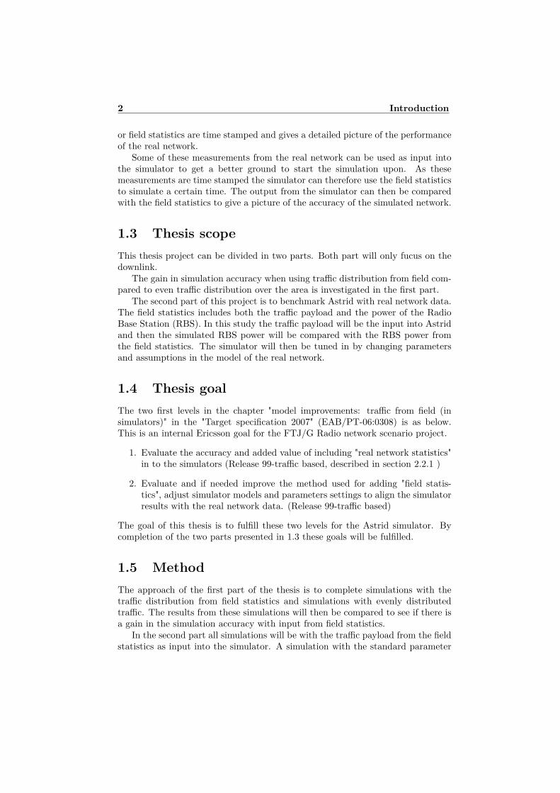
2.1 HistoryIn the 1980’s the first generation mobile systems were introduced. There wereanalog networks for speech services. Several standards were used one of themwas Nordic Mobile Telephones, NMT, which were using the Frequency DivisionMultiple Access (FDMA). In FDMA each user has a portion of the total bandwidthduring the entire transmission as shown to the left in figure 2.1.
Second generation mobile system, which uses digital transmission, were intro-duced in the late 1980’s. These networks covered speech and low bit rate datatransmission. One example of second generation mobile networks is Global Sys-tem for Mobile Communication, GSM, which uses a combination of Time DivisionMultiple Access (TDMA) and FDMA with multiple frequency channels with 8time slots each. In TDMA each user has its own time slot to transmit as shownin the middle of figure 2.1.
The third generation mobile systems, 3G, support a greater number of userswith higher rates then the second generation mobile systems. The goals with 3Gare high-quality multimedia and global roaming. In Europe, the 3G air interface isWideband Code Division Multiple Access (WCDMA). In CDMA systems all usersuse the total bandwidth of the channel all the time and the users are separated byunique codes. [3] [13]
2.2 UMTSThe Universal Mobile Telecommunication System, UMTS, is often called thirdgeneration mobile radio system, 3G. The standards for UMTS have been specifiedby third-generation partnership project, 3GPP, which is a joint standardizationproject for Europe, Korea, Japan, USA and China. Members of the 3GPP arecompanies such as mobile telephony system manufactures and operators.
5
6 Theoretical background
Figure 2.1. Radio Access Technologies
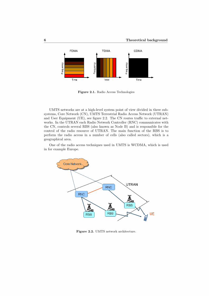
UMTS networks are at a high-level system point of view divided in three sub-systems, Core Network (CN), UMTS Terrestrial Radio Access Network (UTRAN)and User Equipment (UE), see figure 2.2. The CN routes traffic to external net-works. In the UTRAN each Radio Network Controller (RNC) communicates withthe CN, controls several RBS (also known as Node B) and is responsible for thecontrol of the radio resource of UTRAN. The main function of the RBS is toperform the radio access in a number of cells (also called sectors), which is ageographical area.
One of the radio access techniques used in UMTS is WCDMA, which is usedin for example Europe.
Figure 2.2. UMTS network architecture.
2.2 UMTS 7
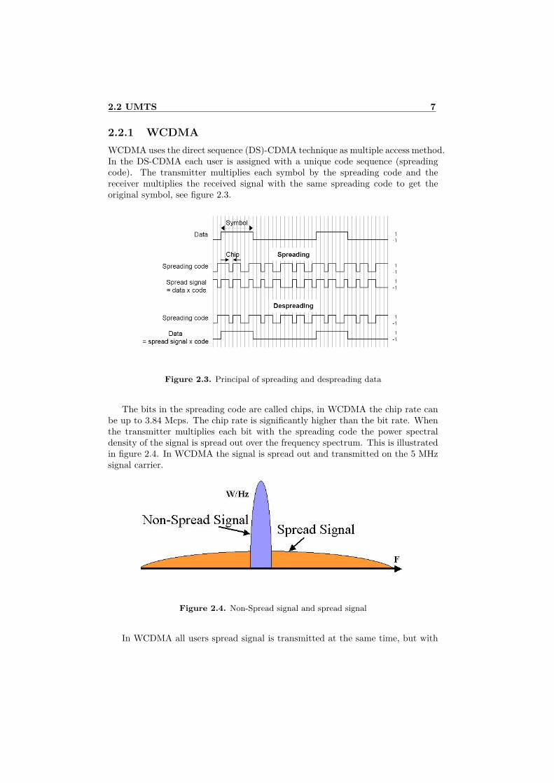
2.2.1 WCDMAWCDMA uses the direct sequence (DS)-CDMA technique as multiple access method.In the DS-CDMA each user is assigned with a unique code sequence (spreadingcode). The transmitter multiplies each symbol by the spreading code and thereceiver multiplies the received signal with the same spreading code to get theoriginal symbol, see figure 2.3.
Figure 2.3. Principal of spreading and despreading data
The bits in the spreading code are called chips, in WCDMA the chip rate canbe up to 3.84 Mcps. The chip rate is significantly higher than the bit rate. Whenthe transmitter multiplies each bit with the spreading code the power spectraldensity of the signal is spread out over the frequency spectrum. This is illustratedin figure 2.4. In WCDMA the signal is spread out and transmitted on the 5 MHzsignal carrier.
Figure 2.4. Non-Spread signal and spread signal
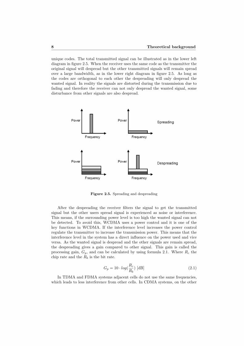
In WCDMA all users spread signal is transmitted at the same time, but with
8 Theoretical background
unique codes. The total transmitted signal can be illustrated as in the lower leftdiagram in figure 2.5. When the receiver uses the same code as the transmitter theoriginal signal will despread but the other transmitted signals will remain spreadover a large bandwidth, as in the lower right diagram in figure 2.5. As long asthe codes are orthogonal to each other the despreading will only despread thewanted signal. In reality the signals are distorted during the transmission due tofading and therefore the receiver can not only despread the wanted signal, somedisturbance from other signals are also despread.
Figure 2.5. Spreading and despreading
After the despreading the receiver filters the signal to get the transmittedsignal but the other users spread signal is experienced as noise or interference.This means, if the surrounding power level is too high the wanted signal can notbe detected. To avoid this, WCDMA uses a power control and it is one of thekey functions in WCDMA. If the interference level increases the power controlregulate the transmitter to increase the transmission power. This means that theinterference level in the system has a direct influence on the power used and viceversa. As the wanted signal is despread and the other signals are remain spread,the despreading gives a gain compared to other signal. This gain is called theprocessing gain, Gp, and can be calculated by using formula 2.1. Where Rc thechip rate and the Rb is the bit rate.
Gp = 10 · log(Rc
Rb) [dB] (2.1)
In TDMA and FDMA systems adjacent cells do not use the same frequencies,which leads to less interference from other cells. In CDMA systems, on the other

2.2 UMTS 9
hand, cells can have the same frequency in each cell, frequency reuse is 1. Themain reason for this is that the signal power is spread out over the frequency bandand therefore it causes less interference.
When a UE moves from one cell to another the UE has to be handed over toanother RBS or sector of a RBS. In TDMA and FDMA system, where adjacentcells do not use the same frequency, the UE must drop the connection before a newradio link can be set up. This is referred to as hard handover and causes a shortinterruption in the connection. When the frequency reuse is 1, as in WCDMA it ispossible to use Soft Handover (SHO). During soft handover the UE is connectedto more than one RBS or RBS sectors at the same time. As each RBS or RBSsector performs power control of the UE in SHO, the SHO reduces the interferencecaused by the UE.
In 1999 the 3GPP released its first version of the WCDMA system standardiza-tion, called Release 99 (R99), the downlink traffic specified in the R99 was CircuitSwitched (CS) 12.2 kbps and 64 kbps and Packet Switched (PS) 64 kbps, 128kbps and 384 kbps. In later releases other traffics have been specified, for exampleHigh Speed Downlink Access (HSDPA) and Enhanced Uplink (EUL), which allowhigher bit rates. [8], [13]
Handover
As written above, WCDMA uses soft handover when a UE moves from one cellto another but there is hard handover in WCDMA as well. In some cells, wherethere are a lot of users, there can be more than one frequency carrier. When a UEis handed over to a new frequency hard handover is used, called inter-frequencyhandover. When a UE moves from an area with WCDMA coverage to anotherarea without WCDMA coverage, for example GSM coverage, hard handover isused, called inter-system handover.
Soft handover can be divided in to two parts, soft and softer handover. Duringsofter hand over the UE is in the overlapping cell coverage area of two or threeadjacent sectors of a RBS. In soft handover the UE is connected to two or moreRBS simultaneously. The difference between softer and soft handover is illustratedin figure 2.6. Softer and soft handover is in this thesis normally called only softhandover, SHO.
The RBSs or RBS sectors that are connected to a UE are called the active setof the UE. If a UE is not in soft handover the active set is only one RBS sector.
In figure 2.7 an illustration of a soft/softer mechanism is shown. An additionalradio link is connected to the UE when the signal strength is within an add margin,which can be set by the network operator. The UE is then connected to two RBSor RBS sectors until one of the radio link’s signal strength gets below a dropthreshold, which is also set by the network operator.
A UE is during SHO assigned to several spreading codes one for each RBS orRBS sector in the active set. The signals from the RBS or RBS sectors in the activeset are received by the UE in SHO as additional multipath components. The onlydifference from multipath reception is that the fingers in the RAKE receiver inthe UE need to generate the respective spreading code for each sector or RBS. A

10 Theoretical background
Figure 2.6. Softer and soft handover
Figure 2.7. Soft handover

2.2 UMTS 11
RAKE receiver separates the individual signals from the multipath reception. Thesignals from cells that are not in the active set are, as before, seen as interference.
Two main advantages with softer and soft handover are that there is smoothertransmission with no momentary interruption during handover and it reduces theinterference in the system. One reason to the reduction in interference with SHO isthat there are more than one RBS that controls the power of the UE. Disadvantagesof softer and soft handover are that it requires a more complex implementationthan hard handover and during the handover more network resources are used,such as power resource and spreading code resource. [8]
Power control
As mention before the power control is perhaps the most important function inWCDMA and its main purpose is to reduce the interference in the system. A singleoverpowered UE could block a whole cell and reduce the capacity in adjacent cells.If one UE is close to the RBS and another UE is on the cell edge, the RBS wouldonly "hear" the closest UE, if there is no power control mechanism.
In WCDMA there are three types of power control loops, fast closed loop-powercontrol, outer loop-power control and the open loop-power control.
The fast power control loop controls the power both for the uplink and downlinkand it is updated 1500 time per second. This is faster than a fast fading couldpossibly happen. The fast power control loop estimates the received Signal toInterference Ratio (SIR) and regulates the SIR towards a SIR target.
The SIR target is controlled by the outer loop power control and it is regulatedto achieve a specific blocking error rate (BLER) target. If the SIR target is toohigh the transmitter uses to much power and there for causes more interferencethan necessary and if it is too low the receiver will not be able to detect the signalwith an accurate BLER. The required SIR depends for example on the multipathprofile and the speed of the UE.
The open loop-power control is used to provide an initial power setting in thebeginning of a connection of a UE. [8] [10]
Lower protocol layers
When a UE and a RNC or RBS communicates it is necessary that the details ofthe communication is well defined in protocols. These protocols can be distributedacross hierarchically arranged layers, see figure 2.8. The three lowest layers inWCDMA are in this thesis the most interesting and they are called Radio ResourceControl layer (RRC), Medium Access Control and Radio Link Control layer (MACand RLC) and the Physical layer (PHY).
The PHY layer, which is the lowest layer (Layer 1), is responsible for trans-mitting data over the physical channels including modulation and spreading.
The MAC and RLC layer (Layer 2) is responsible for the decision making withregards to such things as the data speed and channel coding. It delivers data blockto the PHY layer over the transport channels.
The RRC layer (Layer 3) is the third layer and responsible for radio resourcecontrol including broadcast system information and management of radio connec-

12 Theoretical background
tions. The channel between the RRC layer and the MAC and RLC layer is calledlogical channel. In Appendix H there is more information about logical, transportand physical channels.
In each layer extra bits are added, e.g. headers. This means, when bit ratesare discussed it has to be defined on what layer and if it is before or after theheaders are added. [8]
Figure 2.8. Protocol stack
Channels
In the channels between these three layer and the channels between the transmitterand receiver are mainly two types of channels, dedicated channels and commonchannels. Dedicated channels are specific for each user while the common channelsare shared by all users.
The channel can also be divided in data channels (DCH) and control channels(CCH). The control channels controls the connection and the DCH carries theactual data. The CCH consist of both dedicated and common channels but theDCH consist of only dedicated channels.
The main common control channel (CCCH) is the Common Pilot Channel(CPICH). The CPICH power received by the UE specifies the signal strength fromthe cell. This means, if the power setting of the CPICH is changed the coverageof the cell will be changed. The power setting of the CPICH is normally 10% ofthe RBS power but to optimize a mobile network the power setting of the CPICHcan be tuned in. Other common control channels are set relatively to the CPICH.Hence if the CPICH power is decreased the power used by the other CCCHs arealso decreased.
2.2 UMTS 13
High Speed Downlink Packet Access - HSDPA
As the demand of higher speed in the mobile network increases a greater capacitywill be needed in the WCDMA system. Therefore the HSDPA was introduced inthe WCDMA 3GPP’s release 5. HSDPA will provide peak rates of up to 14 Mbpsand 2-3 times greater capacity. HSDPA is based on five main technologies, shared-channel transmission, higher-order modulation, link adaptation, radio-channel-dependent scheduling and hybrid ARQ with soft combining.
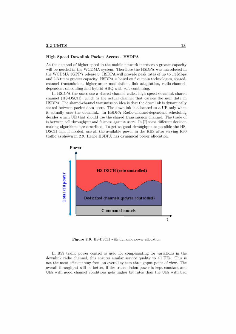
In HSDPA the users use a shared channel called high speed downlink sharedchannel (HS-DSCH), which is the actual channel that carries the user data inHSDPA. The shared-channel transmission idea is that the downlink is dynamicallyshared between packet-data users. The downlink is allocated to a UE only whenit actually uses the downlink. In HSDPA Radio-channel-dependent schedulingdecides which UE that should use the shared transmission channel. The trade ofis between cell throughput and fairness against users. In [7] some different decisionmaking algorithms are described. To get as good throughput as possible the HS-DSCH can, if needed, use all the available power in the RBS after serving R99traffic as shown in 2.9. Hence HSDPA has dynamical power allocation.
Figure 2.9. HS-DSCH with dynamic power allocation
In R99 traffic power control is used for compensating for variations in thedownlink radio channel, this ensures similar service quality to all UEs. This isnot the most efficient way from an overall system-throughput point of view. Theoverall throughput will be better, if the transmission power is kept constant andUEs with good channel conditions gets higher bit rates than the UEs with bad

14 Theoretical background
channel conditions, see figure 2.10. This is often referred to as link adaptation orrate adaptation and is used in HSDPA.
Figure 2.10. Rate adaption
The scheduling and link adaption decision is made every Transmission TimeInterval (TTI), which is in HSDPA 2 ms. With a relatively short TTI the adaptioncan track rapid variation in the radio channels. To increase the throughput evenmore, HSDPA supports both 16-Quadrature Amplitude Modulation (16QAM) andQuadrature Phase Shift Keying (QPSK) modulation. 16QAM carries double asmany bits per symbol than QPSK but 16QAM is less robust than QPSK. There-fore the 16QAM is only used when the radio-channel conditions so allow. Thesemodulations for HSDPA where standardize in 3GPP’s Release 5, in later releasesthe HSDPA will also supports 64QAM.
With Hybrid Automatic Repeat Request (HARQ) the UE stores a failed trans-mission and combine it with the retransmission to increase the probability of suc-cessful decoding. Both R99 and HSDPA use HARQ but the main difference be-tween HSDPA and R99 is that the HARQ in HSDPA is implemented on the MAClayer and the in R99 it is implemented in on the RLC layer, which is above theMAC layer in the protocol stack. This leads to a lower retransmission delay forHSDPA than for R99. [4] [9] [14] [15]
Chapter 3
Network model
This chapter describes how the network is modeled. It starts with the tools used,continues with a description of some simulation models and finishes with an ex-planation of the field statistics handling.
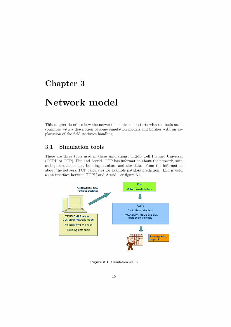
3.1 Simulation toolsThere are three tools used in these simulations, TEMS Cell Planner Universal(TCPU or TCP), Elin and Astrid. TCP has information about the network, suchas high detailed maps, building database and site data. From the informationabout the network TCP calculates for example pathloss prediction. Elin is usedas an interface between TCPU and Astrid, see figure 3.1.
Figure 3.1. Simulation setup
15

16 Network model
Both Astrid and TCPU can simulated mobile networks. Astrid is used becauseit handles future network features that TCPU can not handle at the moment.TCP, Elin and Astrid is described in more detail in section 3.1.1, 3.1.2 and 3.1.3respectively.
3.1.1 TEMS Cell Planner UniversalTEMS Cell Planner Universal is a commercially available product which is usedfor designing, implementing and optimizing mobile radio networks. In these sim-ulations TCP is used together with Elin for creating simulation project in Astrid.In TCPU there is information about the network like site data, maps and buildingdata base. The site data includes for example:
• Location of RBS
• Antenna height, position direction
• Antenna down tilt
• Antenna types
• Feederloss
• RBS maximum power
• Tower mounted amplifier (TMA) information
TCP uses a geographical information system (GIS) called GeoBox. The GISdatabase stores information about the geographical data, the map resolution andcoordinates reference system.
In TCPU high resolution maps, 5m·5m and building database is setup to modelthe real environment. The map resolution area is called a bin and TCP calculatesa pathloss to each bin, see section 3.2.2 for a more detailed description of thepathloss calculations. When the real network is modeled in TCPU the followingdata is exported to Astrid via the Elin interface.
• The pathloss prediction from each RBS to each bin
• Network structure with information about locations of the RBS
• Power settings
• Maps
3.1.2 ElinTo be able to use the output data from TCPU in Astrid the data has to beconformed. This is done by Elin which is a matlab based application. Elin createsan Astrid project in matlab format based on the output data from TCPU.

3.1 Simulation tools 17
3.1.3 AstridAstrid is a matlab based static simulator, which uses Monte Carlo simulations togather statistics. In a static simulator there is no time aspects. Hence the numberof users is constant and the users do not move.
A Monte Carlo simulation is iterative method which uses random input vari-ables to evaluate a deterministic model. For each Monte Carlo iteration the usersare randomly spread out over the area. Results from the iterations, or snapshots,can be average to get more statistical valid results. If there is low traffic densitymany snapshots are needed and if there is high traffic density fewer snapshots canbe used to get a statistic valid result.
It is not possible to spread out the users in three dimensions, in this version ofAstrid. Instead all UEs are assumed to be at the same height level, 1.5 m aboveground level, but in different geographical positions for each iteration.
Astrid models protocol layers up to the RLC layer. This means that the HS-DPA bit rates in this thesis are at the RLC layer, including the RLC layer headerbits.
When simulating a limited area the cells at the border of the area do not getaccurate inter-cell interference. One solution to this problem is to apply wraparound. Wrap around is when copies of the simulation area are placed around theoriginal simulated area. This means that cells at the edge of the simulation areais interfered by the cells on the other side of the simulated area. When simulatingreal networks, as in this thesis work, where the cells have specific position on themap, wrap around can not be applied.
Since the wrap around is not possible a smaller area inside the simulated area isidentified as the analysis area (also called the active area) and the remaining part ofthe simulated area is used to get a proper interference level. In the postprocessingof the result only the active area is filtered out and used in the evaluation.
A bin is a geographical position with the size of the map resolution, 5m·5m.The cell that has the strongest signal in a bin is called the best server cell for thatbin.
A cell is active as long as it is best server in any bin inside the "cluster 2" area.Cluster 2 is an Ericsson internal name of an area in the simulation area.
Traffic payload is only distributed over the active cells (or active area). Theremaining cells are considered as supportive cells and generate interference. Thesecells are not used in the evaluation of the result. The supportive cells use a fixpower, which is set relative to the traffic in the active cells.
Before making a simulation in Astrid some traffic parameters have to be set,these parameters are:
• Traffic density - should be in Erlang/km2.
• Indoor/outdoor distribution - how big part of the traffic should be indoor/outdoor.
• Service distribution - what services should be simulated and with what load.
This version of Astrid can simulated the following traffic.

18 Network model
• R99 - Speech, Video and PS traffic defined in 3GPP Release 99, here calledR99 traffic, Astrid adds SHO traffic for the UEs in SHO.
• HSDPA - The HSDPA traffic load is set by the HSDPA utilization, explainedin Appendix E
• EUL - Enhanced Uplink
• MBMS - Multimedia Broadcast/Multicast Services
This thesis only focuses on R99 and HSDPA traffic. [6]
3.2 Models of signal strengths and interferenceThis section describes how the signal’s propagation from the RBS to the UE (down-link) is modeled in this simulation setup. An overview of the signal’s propagationfrom the RBS to the UE is illustrated in figure 3.2. The signal’s propagation fromthe RBS to the UE can be divided in three parts. The first part is from the top ofthe RBS cabinet to the RBS antenna, described in section 3.2.1. The second partis from the RBS antenna to the UE and it is called the pathloss (or air pathloss),described in section 3.2.2. The third part is the fading due to time variations inthe environment. The fading is described in section 3.2.3.
Figure 3.2. RBS to UE
3.2.1 Pathloss from top of RBS cabinet to RBS antennaThe signal will be affected by the following during the transportation from theRBS to the output side of the RBS antenna.

3.2 Models of signal strengths and interference 19
• Feederloss - due to attenuation in the cable, depends on the length and cabletype.
• TMA - Tower mounted amplifier, gain in uplink and loss in downlink.
• Antenna gain - Depends on the type of antenna.
3.2.2 Air pathloss modelFor simulations of hexagon networks a commonly used air pathloss model is theOkumura-Hata model, which uses the antenna heights of the receiver and trans-mitter, the environment type and the distance to calculate the pathloss betweentwo points.
This simulation setup uses pathloss model called the urban propagation modelinstead. The urban propagation model consists of three models, a half-screenmodel, a recursive micro cell model and a building penetration model. The buildingpenetration model is used for indoor propagation. The other two models are usedfor outdoor propagation.
The pathloss to a bin is calculated by both the outdoor propagation modelsand the model with lowest pathloss is chosen. If it is an indoor bin the indoorpropagation model is added on the outdoor propagation model. This is illustratedin figure 3.3.
Figure 3.3. Propagation model
Outdoor propagation model
In an urban area there are two main paths for the signal to reach the receiver,over rooftops and along streets.
The half-screen model calculates the propagation over rooftops. From theinformation about the environment and obstacles between the transmitter and thereceiver, the half-screen model modulates the obstacles with screens. The screensheight is correlated to the obstacles height. The pathloss is then calculated byusing a multiple knife-edge approach. Information about knife-edge calculationscan be found in [12].
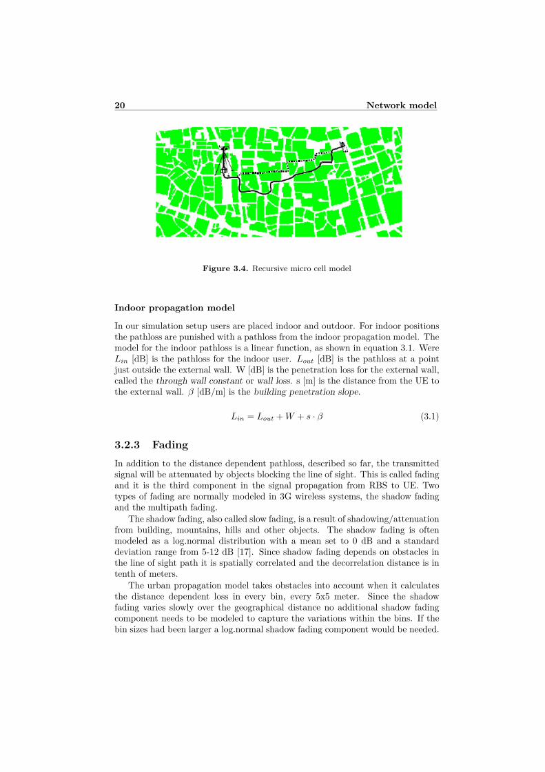
The recursive micro cell model calculates the pathloss between the buildingsand along the streets. The pathloss is calculated by determining the illusorydistance from the RBS antenna to a bin. Figure 3.4 illustrates an example ofdifferent propagation paths along the streets.
20 Network model
Figure 3.4. Recursive micro cell model
Indoor propagation model
In our simulation setup users are placed indoor and outdoor. For indoor positionsthe pathloss are punished with a pathloss from the indoor propagation model. Themodel for the indoor pathloss is a linear function, as shown in equation 3.1. WereLin [dB] is the pathloss for the indoor user. Lout [dB] is the pathloss at a pointjust outside the external wall. W [dB] is the penetration loss for the external wall,called the through wall constant or wall loss. s [m] is the distance from the UE tothe external wall. β [dB/m] is the building penetration slope.
Lin = Lout + W + s · β (3.1)
3.2.3 FadingIn addition to the distance dependent pathloss, described so far, the transmittedsignal will be attenuated by objects blocking the line of sight. This is called fadingand it is the third component in the signal propagation from RBS to UE. Twotypes of fading are normally modeled in 3G wireless systems, the shadow fadingand the multipath fading.
The shadow fading, also called slow fading, is a result of shadowing/attenuationfrom building, mountains, hills and other objects. The shadow fading is oftenmodeled as a log.normal distribution with a mean set to 0 dB and a standarddeviation range from 5-12 dB [17]. Since shadow fading depends on obstacles inthe line of sight path it is spatially correlated and the decorrelation distance is intenth of meters.
The urban propagation model takes obstacles into account when it calculatesthe distance dependent loss in every bin, every 5x5 meter. Since the shadowfading varies slowly over the geographical distance no additional shadow fadingcomponent needs to be modeled to capture the variations within the bins. If thebin sizes had been larger a log.normal shadow fading component would be needed.
3.2 Models of signal strengths and interference 21
When it comes to the multipath fading, it depends on objects in the line ofsite path of the signal but now the fading is due to a number of reflections onlocal surfaces, like part of buildings or smaller objects. A wireless system can bethought of as a collection of rays taking different paths between the transmitterand receiver, giving raise to so called multipath fading.
The received signal will be a sum of copies of the transmitted signal. Thecopies of the transmitted signal reaches the receiver at different time, with dif-ferent pathloss and phase due to varying distance and reflections. This leads tothat signals from different users are not orthogonal to each other at the receiver.The multiple components of the signal may generate constructive or destructiveinterference. Small movements, in order of half wavelengths, can change the con-structive interference into destructive interference or vice versa. Therefore thedecorrelation distance for multipath fading is order of half wavelength.
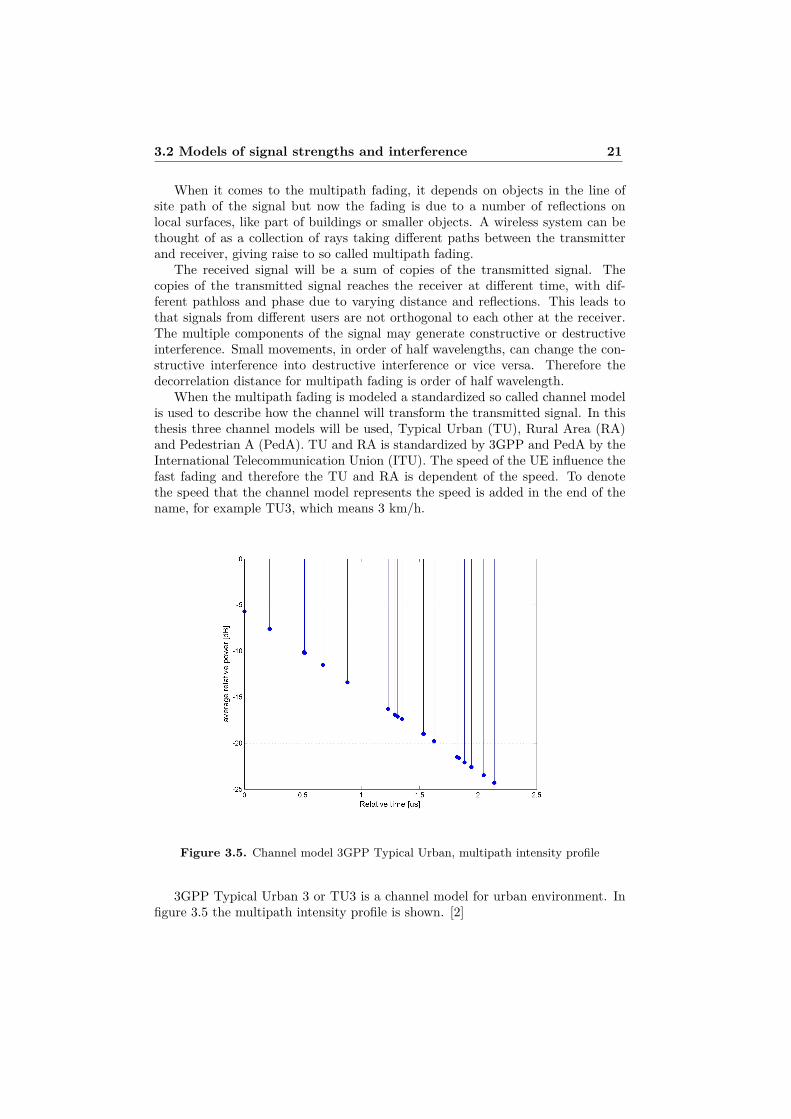
When the multipath fading is modeled a standardized so called channel modelis used to describe how the channel will transform the transmitted signal. In thisthesis three channel models will be used, Typical Urban (TU), Rural Area (RA)and Pedestrian A (PedA). TU and RA is standardized by 3GPP and PedA by theInternational Telecommunication Union (ITU). The speed of the UE influence thefast fading and therefore the TU and RA is dependent of the speed. To denotethe speed that the channel model represents the speed is added in the end of thename, for example TU3, which means 3 km/h.
Figure 3.5. Channel model 3GPP Typical Urban, multipath intensity profile
3GPP Typical Urban 3 or TU3 is a channel model for urban environment. Infigure 3.5 the multipath intensity profile is shown. [2]

22 Network model
In figures 3.6 and 3.7 the multipath intensity profile for Pedestrian A (PedA)and Rural Area (RA) is shown. The RA and PedA has fewer taps then the TU,and this leads to that the TU transforms the signal more than RA and PedA [1].Even if the multipath intensity profile for PedA and RA is not equal to each otherthey are practically similar in a performance estimation point of view, accordingto [5].
Figure 3.6. Channel model Pedestrian A, multipath intensity profile
3.2.4 InterferenceAs described in section 2.2.1 a target for the outer loop power control in WCDMAis the SIR target. The SIR target regulates how strong the signal should bewhen it reaches the receiver. The power of the signal at the receiver depends onthe transmitted power and the pathloss. Hence, the interference depends on thepathloss and the power used by other users.
The SIR target is defined as the energy per bit divided by the interferenceenergy, Eb
I0after the RAKE-combining in the UE. RAKE-combining is when the
receiver combines the multipath signals, which reduce the interference. As differentUEs are not equally good on RAKE combining the Eb/I0 value depends on theUE.
The Ec/N0 is a measure of the coverage in the WCDMA system and is thereforeused when planning a network. In contrast to Eb/I0 the Ec/N0 is defined at theantenna in the UE, before the RAKE-combining. Ec is the energy of the signal

3.2 Models of signal strengths and interference 23
Figure 3.7. Channel model 3GPP Rural Area, multipath intensity profile
(or carrier), the relation between Eb and Ec is described by equation 3.2, whereGp is the processing gain.
Ec = Eb −Gp (3.2)
The Ec/N0 and the Eb/I0 or Ec/I0 is modeled in the simulator as in equation3.3 and 3.4.
Ec
N0=
Ec
Ior + Ioc
=Ec
Ior(1 + Ioc
Ior)
=Ec
Ior
· 11 + G−1
(3.3)
Ec
I0=
Ec
α · Ior + Ioc
=Ec
Ior(α + Ioc
Ior)
=Ec
Ior
· 1α + G−1
(3.4)
As shown in figure 3.8, the Ior is the interference from own cell and Ioc isthe interference from other cell plus the background noise. G = Ior
Iocis called the
geometry factor and it is the relation between interference from own cell and inter-ference from other cells. On the cell boarder G is normally lower than close to theRBS. α is called the nonorthogonality factor and describes the nonorthogonalitybetween signals due to fast fading.
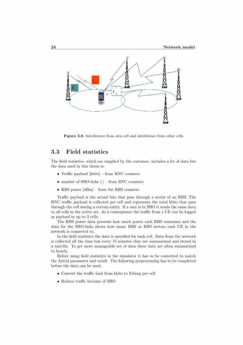
24 Network model
Figure 3.8. Interference from own cell and interference from other cells
3.3 Field statisticsThe field statistics, which are supplied by the costumer, includes a lot of data butthe data used in this thesis is:
• Traffic payload [kbits] – from RNC counters
• number of SHO-links [-] – from RNC counters
• RBS power [dBm] – from the RBS counters
Traffic payload is the actual bits that pass through a sector of an RBS. TheRNC traffic payload is collected per cell and represents the total kbits that passthrough the cell during a certain entity. If a user is in SHO it sends the same datato all cells in the active set. As a consequence the traffic from a UE can be loggedas payload in up to 3 cells.
The RBS power data presents how much power each RBS consumes and thedata for the SHO-links shows how many RBS or RBS sectors each UE in thenetwork is connected to.
In the field statistics the data is specified for each cell. Data from the networkis collected all the time but every 15 minutes they are summarized and stored ina xml-file. To get more manageable set of data these data are often summarizedto hourly.
Before using field statistics in the simulator it has to be converted to matchthe Astrid parameter and result. The following preprocessing has to be completedbefore the data can be used.
• Convert the traffic load from kbits to Erlang per cell
• Reduce traffic because of SHO

3.3 Field statistics 25
• Calculate the service distribution
• Calculate the indoor/outdoor distribution
• Average RBS power data
The two first bullets are illustrated in figure 3.9.
Figure 3.9. Soft handover handling
3.3.1 kbits to Erlang conversionThe unit for the traffic payload from the field statistics counters is kbits, the nameof the counters are presented in Appendix F. This means that the field statisticsshows the downloaded kbits during an hour per cell. As traffic payload in Astridshould be in Erlang per km2 the field statistics traffic payload has to be converted.By using the following formula 3.5 kbits during an hour, R, can be converted toErlang, E. When the number of Erlang is known it is trivial to calculate the Erlangper km2 if the area size is known.
E = R · 1 + DTXgain
kbpstot · 3600(3.5)
The DTXgain is a gain due to that the radio channels between the RBS andthe UE does not transmits all the time, which leads to less interference and anincrease in capacity. In speech for example the UE does not need to transmitas much data when the user is quiet compared to when the users talks. TheDTXgain is calculated by using the activity factor described below. There are twodedicated channels between the RBS and the UE, the Dedicated Traffic Channel(DTCH) and the Dedicated Control Channel (DCCH). The transmission speed ofthe DTCH depends on the service but the transmission speed of the DCCH is 3.4kbps for all services.
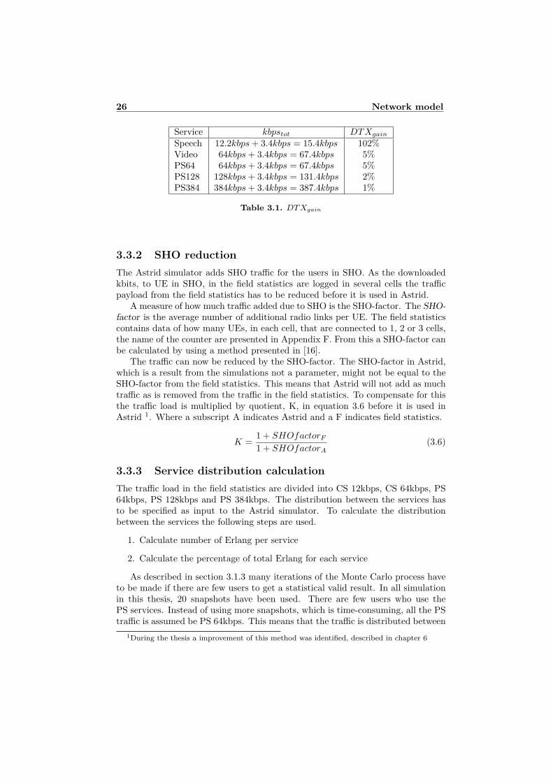
The activity factor tells how big part of the total connection time the UE isactually active. In this thesis the activity factor of the DTCH is assumed to be50% for speech and 100% for all other services, for DCCH the activity factor isassumed to be 10% for all services. These activity factors give the DTXgain shownin table 3.1.
The kbpstot is the total kbps transmitted over the DTCH and DCCH for eachservice. The kbpstot are also shown in table 3.1
26 Network model
Service kbpstot DTXgain
Speech 12.2kbps + 3.4kbps = 15.4kbps 102%Video 64kbps + 3.4kbps = 67.4kbps 5%PS64 64kbps + 3.4kbps = 67.4kbps 5%PS128 128kbps + 3.4kbps = 131.4kbps 2%PS384 384kbps + 3.4kbps = 387.4kbps 1%
Table 3.1. DTXgain
3.3.2 SHO reductionThe Astrid simulator adds SHO traffic for the users in SHO. As the downloadedkbits, to UE in SHO, in the field statistics are logged in several cells the trafficpayload from the field statistics has to be reduced before it is used in Astrid.
A measure of how much traffic added due to SHO is the SHO-factor. The SHO-factor is the average number of additional radio links per UE. The field statisticscontains data of how many UEs, in each cell, that are connected to 1, 2 or 3 cells,the name of the counter are presented in Appendix F. From this a SHO-factor canbe calculated by using a method presented in [16].
The traffic can now be reduced by the SHO-factor. The SHO-factor in Astrid,which is a result from the simulations not a parameter, might not be equal to theSHO-factor from the field statistics. This means that Astrid will not add as muchtraffic as is removed from the traffic in the field statistics. To compensate for thisthe traffic load is multiplied by quotient, K, in equation 3.6 before it is used inAstrid 1. Where a subscript A indicates Astrid and a F indicates field statistics.
K =1 + SHOfactorF
1 + SHOfactorA(3.6)
3.3.3 Service distribution calculationThe traffic load in the field statistics are divided into CS 12kbps, CS 64kbps, PS64kbps, PS 128kbps and PS 384kbps. The distribution between the services hasto be specified as input to the Astrid simulator. To calculate the distributionbetween the services the following steps are used.
1. Calculate number of Erlang per service
2. Calculate the percentage of total Erlang for each service
As described in section 3.1.3 many iterations of the Monte Carlo process haveto be made if there are few users to get a statistical valid result. In all simulationin this thesis, 20 snapshots have been used. There are few users who use thePS services. Instead of using more snapshots, which is time-consuming, all the PStraffic is assumed be PS 64kbps. This means that the traffic is distributed between
1During the thesis a improvement of this method was identified, described in chapter 6
3.3 Field statistics 27
CS 12.2kbps, CS 64kbps and PS 64kbps. CS 64kbps is also a small part of thetotal traffic so it is probably negligible.
3.3.4 Indoor/outdoor calculationsIndoor traffic and outdoor traffic has to be split up in Astrid, but how much ofthe total traffic should be indoor traffic and how much should be outdoor traffic?The customer having the real network uses the assumption that the traffic densityis 4 times higher per km2 in the indoor area than the outdoor area per cell.Therefore this assumption is used in these simulations. Formulas for this methodare presented below. Where A is the area and E is the traffic in Erlang or if it isa km2 in the subscript then is Erlang per km2.
Eout/km2 =Etot
4 ·Ain + Aout(3.7)
Ein/km2 = 4 · Eout/km2 (3.8)
Ein = Ein/km2 ·Ain (3.9)
Eout = Eout/km2 ·Aout (3.10)
The assumption that the traffic is 4 times larger indoor than outdoor can bediscussed if it is correct or not but it will be used in the simulations in this thesis,unless something else is specified.
3.3.5 Average RBS power dataThe counters RBS power is in the field statistics divided in to intervals of 0.5dBm, the name of the counter is presented in Appendix F. The power used in eachcell is measured every 4th second and the field statistics tells how many of thismeasurements that are in each interval. To make an average of the power used byeach cell over an hour each sample in an interval is assumed to be in the middleof the interval. The average power per cell is then converted from dBm to W tomatch the simulated RBS.

28 Network model

Chapter 4
Benchmarking betweenevenly distributed traffic anddistribution from realnetwork data
The traffic load deployed in Astrid can either be specified for the whole area orfor each cell. Earlier the simulations have been completed with the traffic loadspecified for the whole area. When the traffic is specified for the whole area theErlang per km2 is equal in all cells, called even traffic. This lead to that large cellshave large amount of traffic and small cells have small amount of traffic.
In the field statistics the traffic payload is specified for each cell. This canbe used to specify the traffic payload per cell in the simulator. This means thatthe Erlang per km2 is different in different cells, this is called uneven traffic. Theuneven traffic gives a more realistic traffic distribution over the area than witheven traffic.
In this chapter the gain in simulation accuracy, of using uneven traffic as inputinto Astrid compared to even traffic, is investigated.
4.1 Approach
When comparing the results between uneven traffic and even traffic it is importantthat the total amount of traffic is equal in both simulations. To achieve equaltotal traffic the uneven traffic simulation will be made first and the total amountof traffic from this simulation is then used in the even traffic simulation. The bitrates for HSDPA will be used to measure the gain in simulated accuracy withuneven compared to even traffic.
29
30 Benchmarking between evenly distributed traffic and distributionfrom real network data
4.2 Simulated networkThe simulation network in this study is called the City A project and it is anAstrid project with 304 cells and 107 of them are active cells. All of the 304 cellsdo not exist in reality but those which do not exist are by the customer plannedto be alive in the feature. This together with some problems for the customer tocollect the field statistics lead to that the field statistics only includes data for 67of the 107 active cells.
In those 67 cells the average measured traffic is 2.103 Erlang/cell. To theremaining 40 active cells the average of 2.103 Erlang/cell are applied. With thisaverage over 107 cells the total traffic within the active area are 225.05 Erlang(Etot=225.5 Erlang). It would of course be better to use a project where all thesimulated cells exist and it would have been field statistics for all cells but City Awas the best existing project at this time. Collection of new data and updates ofprojects were ongoing.
The active area in City A project contains 240309 bins and with the bin sizeof 25m2 the active area is:
AActive =240309 · 25
106= 6.0077 [km2] (4.1)
Of these 240309 bins there are 109471 indoor bins and 130838 outdoor bins.
Ain =109471 · 25
106= 2.7368 [km2] (4.2)
Aout =130838 · 25
106= 3.2710 [km2] (4.3)
To be able to compare the results from simulations with even and uneven trafficthe total traffic has to be equal. By using Ain, Aout and Etot in equations 3.7-3.8the indoor and outdoor traffic load can be calculated. The outdoor traffic andindoor traffic become 15.83 Erlang/km2 and 63.32 Erlang/km2 respectively forthe even simulation.
As a change in traffic also changes the power consumed it can be interesting tosee how big difference it is in traffic load per cell between even and uneven traffic.A histogram of the difference in Erlang per cell is shown in figure 4.1 and the mostof the cells have less then 1 Erlang in difference when uneven traffic is used insteadof even.
4.3 General simulation configurationThe general simulation configuration in the simulation in this chapter is:
• 5 meter map resolution with 3D building data base
• Realistic network site data (positions, feeder losses, antenna tilts, powersettings. . . )
• Power setting

4.4 Simulations results 31
Figure 4.1. Histogram of difference in Erlang per cell between even and uneven
– Nominal power 17.4 W, 5.5 W for micro cells– CPICH 10% of nominal power– BCH -1.5dB, ref CPICH– PSCH -0.2dB, ref CPICH– BCH -2.1dB, ref CPICH
• Path loss prediction with the Urban propagation model
– Best of Half screen and Micro cell model– The indoor model use 12 dB wall loss and 0.8 dB/m building penetra-
tion slope
• Channel model, TU and PedA
• UE antenna height 1.5 m
• UE category 6
4.4 Simulations resultsIn this section the results from simulations for the City A project with even anduneven traffic are compared. The HSDPA bit rate depends on the available HSDPA
32 Benchmarking between evenly distributed traffic and distributionfrom real network data
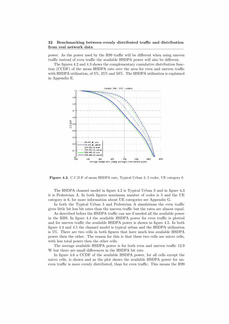
power. As the power used by the R99 traffic will be different when using uneventraffic instead of even traffic the available HSDPA power will also be different.
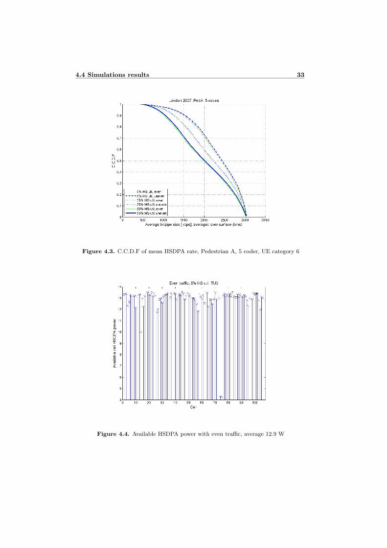
The figures 4.2 and 4.3 shows the complementary cumulative distribution func-tion (CCDF) of the mean HSDPA rate over the area for even and uneven trafficwith HSDPA utilization, of 5%, 25% and 50%. The HSDPA utilization is explainedin Appendix E.
Figure 4.2. C.C.D.F of mean HSDPA rate, Typical Urban 3, 5 coder, UE category 6
The HSDPA channel model in figure 4.2 is Typical Urban 3 and in figure 4.3it is Pedestrian A. In both figures maximum number of codes is 5 and the UEcategory is 6, for more information about UE categories see Appendix G.
In both the Typical Urban 3 and Pedestrian A simulations the even trafficgives little bit less bit rates than the uneven traffic but the rates are almost equal.
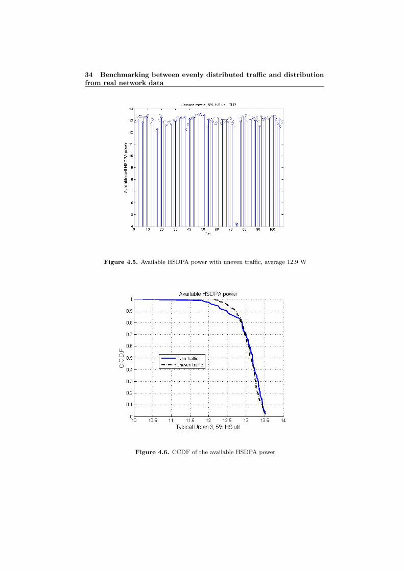
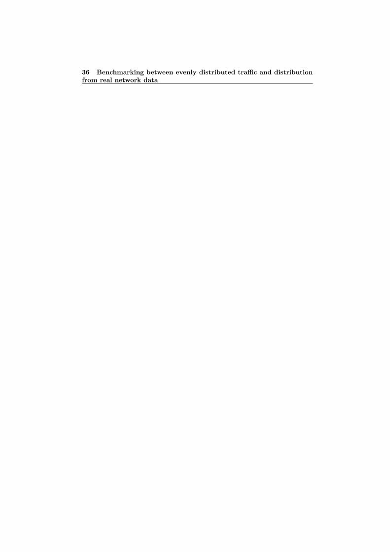
As described before the HSDPA traffic can use if needed all the available powerin the RBS. In figure 4.4 the available HSDPA power for even traffic is plottedand for uneven traffic the available HSDPA power is shown in figure 4.5. In bothfigure 4.4 and 4.5 the channel model is typical urban and the HSDPA utilizationis 5%. There are two cells in both figures that have much less available HSDPApower then the other. The reason for this is that these two cells are micro cells,with less total power then the other cells.
The average available HSDPA power is for both even and uneven traffic 12.9W but there are small differences in the HSDPA bit rate.
In figure 4.6 a CCDF of the available HSDPA power, for all cells except themicro cells, is shown and as the plot shows the available HSDPA power for un-even traffic is more evenly distributed, than for even traffic. This means the R99
4.4 Simulations results 33
Figure 4.3. C.C.D.F of mean HSDPA rate, Pedestrian A, 5 coder, UE category 6
Figure 4.4. Available HSDPA power with even traffic, average 12.9 W
34 Benchmarking between evenly distributed traffic and distributionfrom real network data
Figure 4.5. Available HSDPA power with uneven traffic, average 12.9 W
Figure 4.6. CCDF of the available HSDPA power

4.5 Summary of results 35
power also is more evenly distributed over the cells for uneven traffic. Networkplanners strive to place the antenna sites to achieve good coverage but they alsodo small cells where they believe there will be a lot of traffic to get the trafficevenly distributed over the cells. This indicates that the simulated network is wellplanned.
4.5 Summary of resultsDue to that there were only payload data for 67 of 107 cells and the remaining 40cells got an average traffic load the results gives only a hint of the actual result ofusing uneven traffic instead of even traffic as input into Astrid. It would of coursebeen more reliable if there would have been data for all the cells.
In the City A project network with payload data for 63% of the cells there isno gain of using uneven traffic instead of even traffic with today’s traffic load. Theresulting HSDPA bit rates will be almost equal. In the future when the traffic loadhas increased it can be more difference between the results with even and uneventraffic. This means that in the future there will probably more gain in simulationaccuracy of using uneven traffic.
To get rid of the problem with the nonexisting cells a new project, City 2007D, was created with out these nonexisting cells. It would be interesting to seeif there would be larger difference in the HSDPA bit rates with the City 2007 Dproject, where all cells are alive. This is matter for further studies.
36 Benchmarking between evenly distributed traffic and distributionfrom real network data
Chapter 5
Benchmarking of RBS powerbetween simulation resultand field data
In this chapter Astrid will be benchmarked with real network data from customer’snetwork in a European city. The traffic payload from field is used as input trafficinto Astrid and the simulated power of the RBSs are then compared with fieldstatistics for the RBS power, which is synchronized in time with the field statisticsfor the traffic payload.
5.1 ApproachThe measured RBS power and traffic payload is synchronized in time, meaningthat they are measured during the same time interval. The measured traffic pay-load per cell will be used to configure the traffic demand in the Astrid simulator.During the simulation Astrid generates RBS power, based on the traffic payloadper cell. The simulated RBS power will than be compared with the measured RBSpower, to estimates accuracy in the simulator. If the simulated RBS power is notclose enough to the measured value an investigation will be completed to identifythe main reasons for the difference in RBS power. From this investigation somepossible explanations to the power difference will be suggested and evaluated. Itwill be an iterative process to tune in the RBS is modeled more accurately. Witha more accurate simulated RBS power, the pathloss, interference and thus theoverall simulation result is more likely to be more accurate than before.
5.2 Simulated networkAs explained in chapter 4 the City A project has more cells than in reality. To beable to compare the real network with the simulated network a new project was
37

38 Benchmarking of RBS power between simulation result and fielddata
created, called City D, where the nonexisting cells are removed. City D projectconsist of 228 cells and 85 of them are active. The simulated area and the analyzedarea is the same as in the City A project. When comparing the traffic payloadwith the cells in City D an additional RBS was identified as nonexisting, includingtwo active cells and one supportive cell. To remove the nonexisting cell in the CityD project would imply that the whole chain of creating a new project has to beredone. This was something we wanted to avoid to start with.
For the RBS power data, the data collection is more difficult than for the RNCdata, and it was only possible to get RBS data for 50 of the 85 active cells.
In the traffic payload data, there were data for all existing cells except for one.The costumer, who supplies the field statistics, had problems to get the trafficpayload data from this cell.
What traffic payload should be applied to the cells without traffic payload data?For the two active cells that do not exist in reality there are two main options.One way is to use the average traffic payload but then the total number of usersin the system would be larger in the simulations than in reality and therefore theinterference level might be larger than in reality. Another way is to set the trafficpayload to 0, this might lead to an lower interference level than in reality.
The second option is used in this simulations since the cell do not exist. Thereis one active cell that do exist in reality but do not have traffic payload data andfor this cell an average traffic payload is applied.
5.3 General simulation configurationThe general simulation configuration in the simulation in this chapter is presentedbelow. These are the values used unless other values are specified.
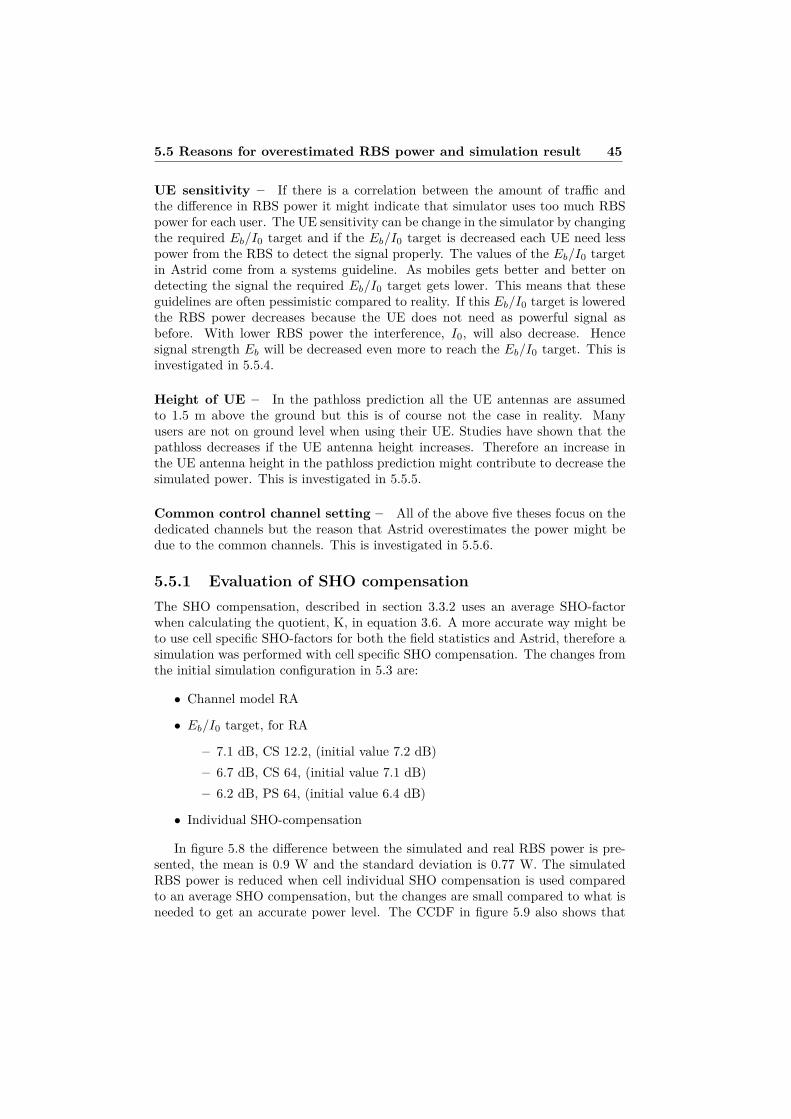
• 5 meter map resolution with 3D building data base
• Realistic network site data (positions, feeder losses, antenna tilts, powersettings. . . )
• Power setting
– Nominal power 17.4 W, 5.5 W for micro cells– CPICH 10% of nominal power– BCH -1.5 dB, rel. CPICH– PSCH -0.2 dB, rel. CPICH– SSCH -2.1 dB, rel. CPICH
• Path loss prediction with the Urban propagation model
– Best of Half screen and Micro cell model– The indoor model use 12 dB wall loss and 0.8 dB/m building penetra-
tion slope
• Eb/I0 targets, for TU

5.4 Initial simulation results 39
– 7.2 dB, CS 12.2– 7.1 dB, CS 64– 6.4 dB, PS 64
• Channel model, TU
• UE antenna height, 1.5 m
• Traffic distribution, indoor traffic per km2 = 4·outdoor traffic per km2
• Average SHO-compensation
5.4 Initial simulation results
Figure 5.1. Difference in RBS power, simulated - real, channel model TU3
To get a first overview of how accurate the simulated RBS power is comparedto the real RBS power a simulation was made with the general simulation config-uration as described in section 5.3, which is a commonly used setting in Astrid.In the figure 5.1 the difference between the simulated and the real RBS power isshown. In most of the cells the measured RBS power is lower than the simulatedRBS power. The mean of the difference is 1.1 W and the standard deviation is0.83 W. The ideal would be to have the mean of 0 W and a standard deviation of0 W.

40 Benchmarking of RBS power between simulation result and fielddata
Figure 5.2. CCDF of the difference in RBS power, initial setting
In figure 5.2 the CCDF of the difference in RBS power is shown together withthe ideal CCDF and it shows that the simulator generally overestimates the RBSpower given a certain traffic load.
5.4.1 Rural area vs. Typical UrbanIn the parameter setting used in the first simulation the channel model was TypicalUrban. Orthogonality measurements, have during 2006 been performed in urbanand dense urban areas. The measurements are presented in [11]. One of theoutcomes was that the TU3 model is too pessimistic. Instead a Rural Area modelwould be more accurate. Therefore the channel model was changed to a RuralArea. The changes from the initial simulation configuration in 5.3 are:
• Channel model RA
• Eb/I0 target, for RA
– 7.1 dB, CS 12.2, (initial value 7.2 dB)– 6.7 dB, CS 64, (initial value 7.1 dB)– 6.2 dB, PS 64, (initial value 6.4 dB)
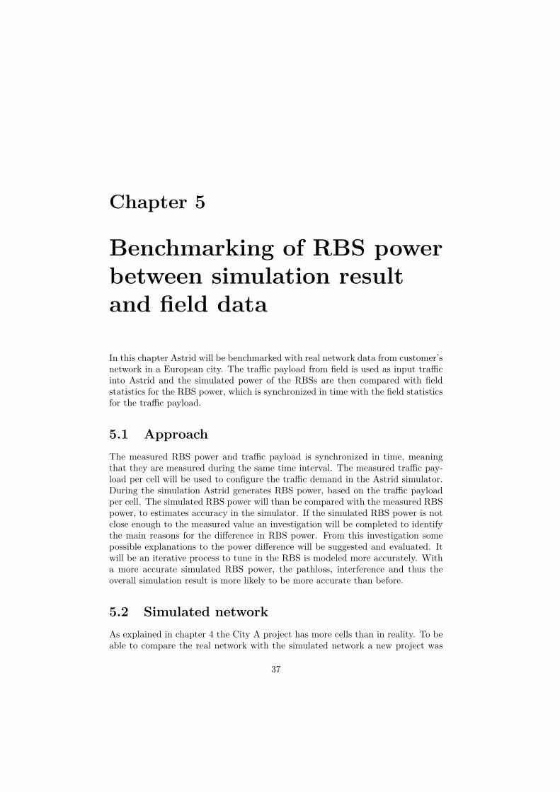
In figure 5.3 the difference in RBS power is shown. Some cells have decreasedtheir simulated power, for example cell 49, and some have larger simulated powerwith RA compared to TU, for example cell 16. In figure 5.4 the CCDFs of the
5.4 Initial simulation results 41
Figure 5.3. Difference in RBS power, simulated - real, channel model RA3
Figure 5.4. CCDF of the difference in RBS power, Rural Area

42 Benchmarking of RBS power between simulation result and fielddata
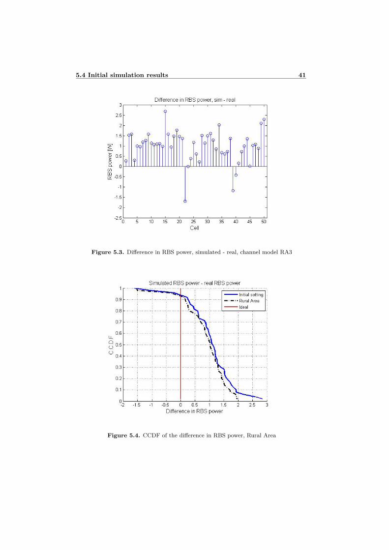
simulation with initial setting and with Rural Area as channel model is shown.This plot shows that the RA is a little bit better than TU in this simulationenvironment. The average difference has decreased, the mean difference is now to1.0 W and the standard deviation 0.78 W. This means, the simulator gives a moreaccurate result when the RA is used instead of TU. Therefore from now on all thesimulations in this thesis were made with the RA as channel model.
5.4.2 Reasons for two deviating cellsIn both figures 5.1 and 5.3 there are two cells, cell number 22 and 39, that deviatefrom the other cells. Both of them have more than 1 W too low simulated power.
Figure 5.5 shows a map with the RBSs over the simulated area and cluster2 area is marked. The two cells with low simulated power are marked with arectangle and a triangle. One of them (cell 22, triangle) is in the outer region thesimulated area. This means that cell 22 has less surrounding cells in the simulatorthan in reality. Cell 22 has therefore too little interference from other cells in thesimulator. Cell number 39 (rectangle) is not on the edge of the simulated area, ithas many surrounding cells. Other reasons have to be found to explain the toolow simulated power.
Figure 5.5. Map over simulated network, cluster 2 area
The, in reality, nonexisting RBS is the RBS marked with a circle, its cells

5.5 Reasons for overestimated RBS power and simulation result 43
therefore have no traffic, as explained in section 5.2. This might lead to that theadjacent cells do not have an accurate interference level. Cell 39 is pretty close tothe nonexisting RBS and this might be a reason for the low simulated power. Toget rid of the problem with the nonexisting cells a new project was created withoutthese three cells, two of them are active cells. The new project (City D no1630)therefore has 225 cells with 83 active cells. With this new project the differencein RBS power is as shown in figure 5.6, mean 1.0 W and standard deviation 0.76W. The mean and the standard deviation is almost unchanged and cell 39 hasonly a little bit more simulated power. The new project did not affect cell 39 asmuch as expected. At the time of writing no explanation found to why Astridunderestimates the RBS power in cell 39, further studies are needed. The City Dno1630 project is used in the subsequent simulations.
Figure 5.6. Difference in RBS power, simulated - real, City D no 1630
As the simulated power for cell 22 and 39 is less than the in reality, theircontribution to interference to adjacent cells are not enough.
5.5 Reasons for overestimated RBS power andsimulation result
The average simulated power was about 1 W too high and to investigate the size ofthe loss needed to get an accurate average simulated power an extra loss componentwas implemented in the simulator. With the extra loss component set to -1.5 dBthe average difference in RBS power was 0.05 W. In figure 5.7 the difference in

44 Benchmarking of RBS power between simulation result and fielddata
RBS power for each cell is presented. This indicates that it is in average of about1.5 dB too much power used in the link budget.
Figure 5.7. Difference in RBS power, simulated - real, loss -1.5 dB
What can be the reason for the 1.5 dB? After some discussion and brain storm-ing six areas where identified that can contribute to the over estimated RBS power.The overestimated RBS power is probably not due to one of these areas, it is morelikely to be a combination.
SHO compensation – In the calculations of the SHO compensation, describedin 3.3.2, the SHO-factors have been the average SHO-factor for all cells. As theSHO-factor varies between each cell it would probably be more accurate to usecell specific SHO-factors in the SHO compensations. This is investigated in 5.5.1.
Indoor propagation model – If a correlation between the difference in RBSpower and indoor area can be found then the indoor propagation model and in-door/outdoor traffic distribution might not be accurate. The indoor model mighthave too high through wall constant or building penetration slope. This is inves-tigated in 5.5.2.
Indoor/outdoor traffic distribution – A correlation between the differencein RBS power and indoor area can also indicate that the indoor/outdoor trafficdistribution assumption might overestimate the indoor traffic and underestimatethe outdoor traffic. This is investigated in 5.5.3.
5.5 Reasons for overestimated RBS power and simulation result 45
UE sensitivity – If there is a correlation between the amount of traffic andthe difference in RBS power it might indicate that simulator uses too much RBSpower for each user. The UE sensitivity can be change in the simulator by changingthe required Eb/I0 target and if the Eb/I0 target is decreased each UE need lesspower from the RBS to detect the signal properly. The values of the Eb/I0 targetin Astrid come from a systems guideline. As mobiles gets better and better ondetecting the signal the required Eb/I0 target gets lower. This means that theseguidelines are often pessimistic compared to reality. If this Eb/I0 target is loweredthe RBS power decreases because the UE does not need as powerful signal asbefore. With lower RBS power the interference, I0, will also decrease. Hencesignal strength Eb will be decreased even more to reach the Eb/I0 target. This isinvestigated in 5.5.4.
Height of UE – In the pathloss prediction all the UE antennas are assumedto 1.5 m above the ground but this is of course not the case in reality. Manyusers are not on ground level when using their UE. Studies have shown that thepathloss decreases if the UE antenna height increases. Therefore an increase inthe UE antenna height in the pathloss prediction might contribute to decrease thesimulated power. This is investigated in 5.5.5.
Common control channel setting – All of the above five theses focus on thededicated channels but the reason that Astrid overestimates the power might bedue to the common channels. This is investigated in 5.5.6.
5.5.1 Evaluation of SHO compensationThe SHO compensation, described in section 3.3.2 uses an average SHO-factorwhen calculating the quotient, K, in equation 3.6. A more accurate way might beto use cell specific SHO-factors for both the field statistics and Astrid, therefore asimulation was performed with cell specific SHO compensation. The changes fromthe initial simulation configuration in 5.3 are:
• Channel model RA
• Eb/I0 target, for RA
– 7.1 dB, CS 12.2, (initial value 7.2 dB)– 6.7 dB, CS 64, (initial value 7.1 dB)– 6.2 dB, PS 64, (initial value 6.4 dB)
• Individual SHO-compensation
In figure 5.8 the difference between the simulated and real RBS power is pre-sented, the mean is 0.9 W and the standard deviation is 0.77 W. The simulatedRBS power is reduced when cell individual SHO compensation is used comparedto an average SHO compensation, but the changes are small compared to what isneeded to get an accurate power level. The CCDF in figure 5.9 also shows that

46 Benchmarking of RBS power between simulation result and fielddata
Figure 5.8. Difference in RBS power, simulated - real, individual SHO
Figure 5.9. CCDF of the difference in RBS power, individual SHO

5.5 Reasons for overestimated RBS power and simulation result 47
there is only a small difference compared to the simulation with the initial settingin section 5.3. The main part of the difference comes from the channel modelchange from Rural Area instead of Typical Urban. Individual SHO-compensationis used in subsequent simulations.
5.5.2 Evaluation of indoor propagation modelIf there is a correlation between indoor/outdoor area distribution and the RBSpower it might indicate that the parameter setting need to be changes for theindoor propagation model, described in section 3.2.2. In figure 5.10 the distributionbetween indoor and outdoor area is shown. By comparing figure 5.10 with figure5.6 a correlation between the indoor/outdoor area distribution and the differencein RBS power can be seen for the cells 14, 15, 21, 25, 34 and 49. These cells havelarge indoor part and high difference in RBS power. There are cells that do nothave this correlation, for example cell 41.
Figure 5.10. (Indoor Area - Outdoor Area)/Total Area, per cell
The overestimated RBS power is, as explained in the beginning of section 5.5,most likely a combination several identified areas. Therefore correlation betweenindoor/outdoor area distribution and the difference in RBS power is strong enoughto justify a test of the change of the parameters in the indoor model.
To investigate if the indoor model is accurate a simulation with a smallerthrough wall constant was completed. As there is 1.5 dB in average too much lossused in the link budget the through wall constant, W in equation 3.1, was changefrom 12 dB to 10 dB. Changes from the initial simulation configuration in 5.3 are:
48 Benchmarking of RBS power between simulation result and fielddata
• Channel model RA
• Indoor model, wall loss 10 dB, (initial value 12 dB)
• Eb/I0 target, for RA
– 7.1 dB, CS 12.2, (initial value 7.2 dB)
– 6.7 dB, CS 64, (initial value 7.1 dB)
– 6.2 dB, PS 64, (initial value 6.4 dB)
• Individual SHO-compensation
Figure 5.11. Difference in RBS power, simulated - real, wall loss 10 dB
The most of the users are indoors, and therefore they are affected by this throughwall constant change, which should lead to a significant change in the simulatedRBS power. The result from this simulation is shown in figure 5.11 and in figure5.12. The average difference in RBS power is now 0.9 W and standard deviationis 0.72 W and the CCDF differs not too much from the base case. The main partof the difference between the RBS power in this simulation and in the initial caseis due to change of channel model. The simulated RBS power did not decrease asmuch as expected. This shows that the indoor model has only a small impact onthe simulated power with today’s traffic load.
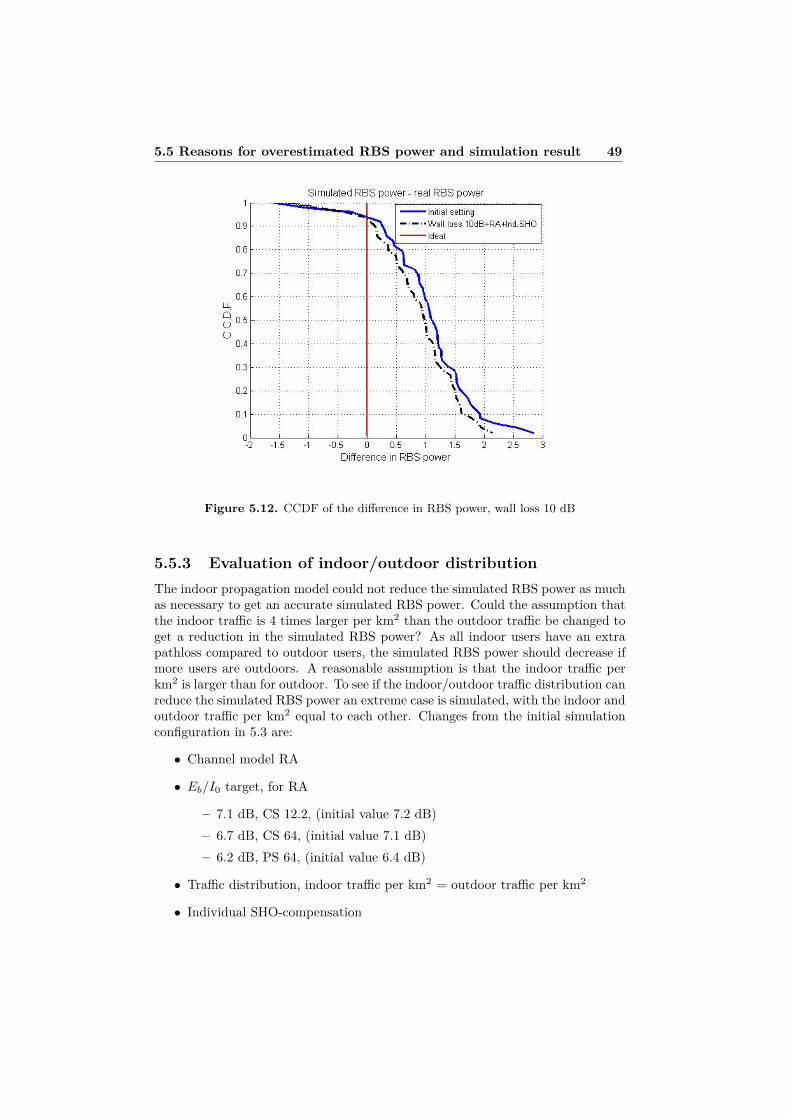
5.5 Reasons for overestimated RBS power and simulation result 49
Figure 5.12. CCDF of the difference in RBS power, wall loss 10 dB
5.5.3 Evaluation of indoor/outdoor distributionThe indoor propagation model could not reduce the simulated RBS power as muchas necessary to get an accurate simulated RBS power. Could the assumption thatthe indoor traffic is 4 times larger per km2 than the outdoor traffic be changed toget a reduction in the simulated RBS power? As all indoor users have an extrapathloss compared to outdoor users, the simulated RBS power should decrease ifmore users are outdoors. A reasonable assumption is that the indoor traffic perkm2 is larger than for outdoor. To see if the indoor/outdoor traffic distribution canreduce the simulated RBS power an extreme case is simulated, with the indoor andoutdoor traffic per km2 equal to each other. Changes from the initial simulationconfiguration in 5.3 are:
• Channel model RA
• Eb/I0 target, for RA
– 7.1 dB, CS 12.2, (initial value 7.2 dB)– 6.7 dB, CS 64, (initial value 7.1 dB)– 6.2 dB, PS 64, (initial value 6.4 dB)
• Traffic distribution, indoor traffic per km2 = outdoor traffic per km2
• Individual SHO-compensation
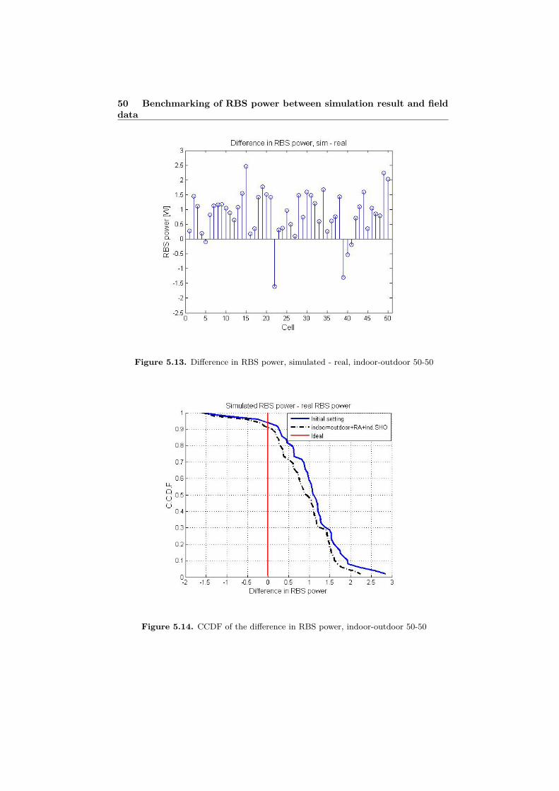
50 Benchmarking of RBS power between simulation result and fielddata
Figure 5.13. Difference in RBS power, simulated - real, indoor-outdoor 50-50
Figure 5.14. CCDF of the difference in RBS power, indoor-outdoor 50-50
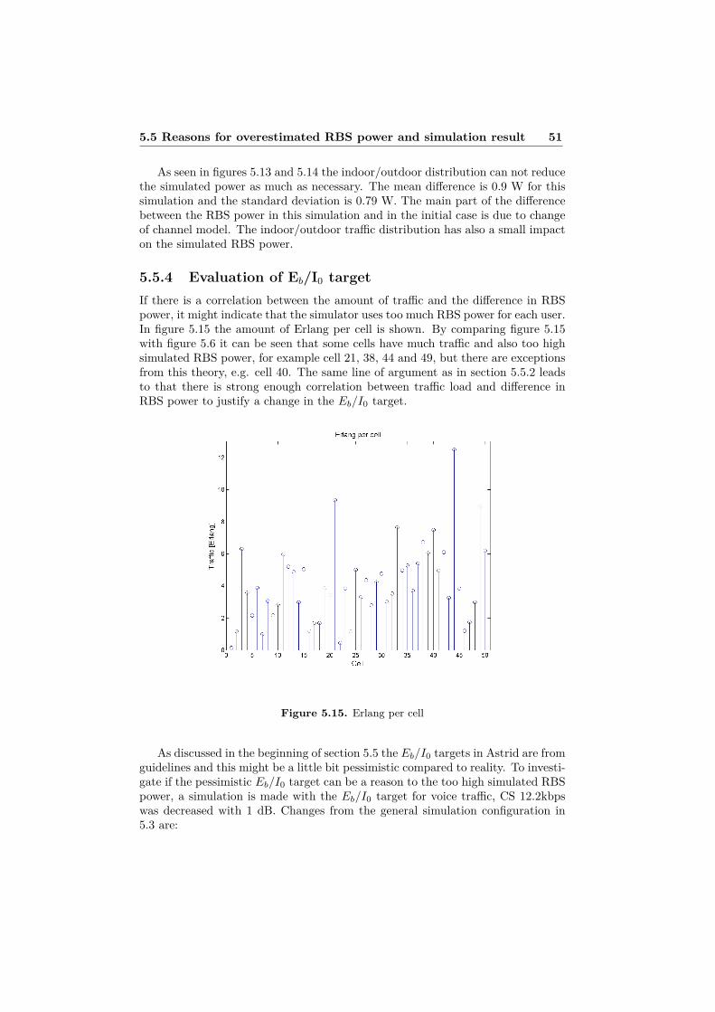
5.5 Reasons for overestimated RBS power and simulation result 51
As seen in figures 5.13 and 5.14 the indoor/outdoor distribution can not reducethe simulated power as much as necessary. The mean difference is 0.9 W for thissimulation and the standard deviation is 0.79 W. The main part of the differencebetween the RBS power in this simulation and in the initial case is due to changeof channel model. The indoor/outdoor traffic distribution has also a small impacton the simulated RBS power.
5.5.4 Evaluation of Eb/I0 targetIf there is a correlation between the amount of traffic and the difference in RBSpower, it might indicate that the simulator uses too much RBS power for each user.In figure 5.15 the amount of Erlang per cell is shown. By comparing figure 5.15with figure 5.6 it can be seen that some cells have much traffic and also too highsimulated RBS power, for example cell 21, 38, 44 and 49, but there are exceptionsfrom this theory, e.g. cell 40. The same line of argument as in section 5.5.2 leadsto that there is strong enough correlation between traffic load and difference inRBS power to justify a change in the Eb/I0 target.
Figure 5.15. Erlang per cell
As discussed in the beginning of section 5.5 the Eb/I0 targets in Astrid are fromguidelines and this might be a little bit pessimistic compared to reality. To investi-gate if the pessimistic Eb/I0 target can be a reason to the too high simulated RBSpower, a simulation is made with the Eb/I0 target for voice traffic, CS 12.2kbpswas decreased with 1 dB. Changes from the general simulation configuration in5.3 are:
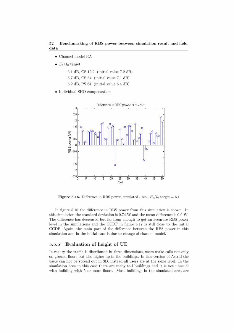
52 Benchmarking of RBS power between simulation result and fielddata
• Channel model RA
• Eb/I0 target
– 6.1 dB, CS 12.2, (initial value 7.2 dB)– 6.7 dB, CS 64, (initial value 7.1 dB)– 6.2 dB, PS 64, (initial value 6.4 dB)
• Individual SHO-compensation
Figure 5.16. Difference in RBS power, simulated - real, Eb/I0 target = 6.1
In figure 5.16 the difference in RBS power from this simulation is shown. Inthis simulation the standard deviation is 0.74 W and the mean difference is 0.9 W.The difference has decreased but far from enough to get an accurate RBS powerlevel in the simulations and the CCDF in figure 5.17 is still close to the initialCCDF. Again, the main part of the difference between the RBS power in thissimulation and in the initial case is due to change of channel model.
5.5.5 Evaluation of height of UEIn reality the traffic is distributed in three dimensions, users make calls not onlyon ground floors but also higher up in the buildings. In this version of Astrid theusers can not be spread out in 3D, instead all users are at the same level. In thesimulation area in this case there are many tall buildings and it is not unusualwith building with 5 or more floors. Most buildings in the simulated area are

5.5 Reasons for overestimated RBS power and simulation result 53
Figure 5.17. CCDF of the difference in RBS power, Eb/I0 target = 6.1
between 12-22 m high. From this the average UE height is estimated to be 8 mabove ground level. In this simulation the changes from the general simulationconfiguration in 5.3 are:
• Channel model RA
• Eb/I0 target, for RA
– 7.1 dB, CS 12.2, (initial value 7.2 dB)
– 6.7 dB, CS 64, (initial value 7.1 dB)
– 6.2 dB, PS 64, (initial value 6.4 dB)
• UE antenna height 8 m, (initial value 1.5 m)
• Individual SHO-compensation
The result from this simulation is shown in figure 5.18. The average differencein RBS power in this simulation is 0.9 W and standard deviation is 0.76 W. TheUE antenna height did not make a major impact on the simulated RBS power ascan be seen in the CCDF in figure 5.19. Again, the main part of the differencebetween the RBS power in this simulation and in the initial case is due to changeof channel model.

54 Benchmarking of RBS power between simulation result and fielddata
Figure 5.18. Difference in RBS power, simulated - real, UE antenna height 8 m
Figure 5.19. CCDF of the difference in RBS power, UE antenna height 8 m

5.5 Reasons for overestimated RBS power and simulation result 55
5.5.6 Evaluation of common control channel settingsThe channels in the downlink can be divided into dedicated channels and commonchannel. The dedicated channels are specific to each user. Therefore the powerused in the RBS for these channels depends for example on the number of users.For the common channels the RBS uses the same power no matter what. Theearlier attempts to decrease the RBS power by only changing the RBS powerused in the dedicated channels but there might be the common channels that aremodeled to use too much power.
The channels can also be divided in data channels (DCH) and control chan-nels (CCH). The data channels, which transport the actual data, are all of themdedicated channels, the control channels are both dedicated and common channels.
Figure 5.20. Control Channel (CCH) power
In figure 5.20 the simulated CCH power is plotted and in figure 5.21 the sim-ulated DCH power is plotted. As these plots show the control channels use muchmore power. The average power used by the DCH is only 0.5 W and the meanpower for the CCH is 3.4 W. Out of the simulated CCH the common channelsuse 3.1 W. This means the dedicated channels use in average 0.8 W. Even if allthe dedicated channels would have been removed (=no users in the network) thesimulated power would have been too high. The earlier attempts to reduce thesimulated power have all been focusing on the dedicated channels and the reasonto that the RBS power has not been reduced as much as expected is that thededicated channels are such a small part of the total power. It would probablybeen better to start to investigate if it is the dedicated or common channels that
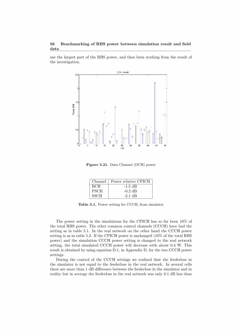
56 Benchmarking of RBS power between simulation result and fielddata
use the largest part of the RBS power, and then been working from the result ofthe investigation.
Figure 5.21. Data Channel (DCH) power
Channel Power relative CPICHBCH -1.5 dBPSCH -0.2 dBSSCH -2.1 dB
Table 5.1. Power setting for CCCH, from simulator
The power setting in the simulations for the CPICH has so far been 10% ofthe total RBS power. The other common control channels (CCCH) have had thesetting as in table 5.1. In the real network on the other hand the CCCH powersetting is as in table 5.2. If the CPICH power is unchanged (10% of the total RBSpower) and the simulation CCCH power setting is changed to the real networksetting, the total simulated CCCH power will decrease with about 0.4 W. Thisresult is obtained by using equation D.1, in Appendix D, for the two CCCH powersettings.
During the control of the CCCH settings we realized that the feederloss inthe simulator is not equal to the feederloss in the real network. In several cellsthere are more than 1 dB difference between the feederloss in the simulator and inreality but in average the feederloss in the real network was only 0.1 dB less than

5.6 Summary of results 57
Channel Power relative CPICHBCH -3.1 dBPSCH -1.8 dBSSCH -3.5 dB
Table 5.2. Power setting for CCCH, from from field
the average feederloss in the simulator. Therefore a simulation with the followingchanges from the general simulation configuration in 5.3 was completed.
• Channel model RA,
• Power setting
– BCH -3.1 dB, rel. CPICH, (initial value -1.5 dB)– PSCH -1.8 dB, rel. CPICH, (initial value -0.2 dB)– SSCH -3.5 dB, rel. CPICH, (initial value -2.1 dB)
• Eb/I0 target, for RA
– 7.1 dB, CS 12.2, (initial value 7.2 dB)– 6.7 dB, CS 64, (initial value 7.1 dB)– 6.2 dB, PS 64, (initial value 6.4 dB)
• Changed values for feederloss, cell individual
• Individual SHO-compensation
The difference in RBS power, from the simulation with the new feederlossesand new CCCH setting (CPICH unchanged), is shown in figure 5.22. The averagedifference in RBS power is now 0.5 W and the standard deviation is 0.78 W. Thesimulated power is more accurate with the right common control channel setting(CCCH) and the accurate feederloss but the deviation is unchanged. The CCDFin figure 5.23 is now considerably closer to the ideal than in the initial simulation.
5.6 Summary of resultsWith the general simulation configuration, presented in section 5.3, the simulatoroverestimated the RBS power with about 1 W in average.
In a study presented in [11] shows that city centers are more behaving like aRural Area channel model compared to Typical Urban. The simulation result insection 5.4.1 confirms the study results in [11], in regards to power consumption.
One of the reasons to the overestimated the RBS power was that the CCCHsettings in the simulator were not equal to the CCCH setting in the real network.With the right CCCH setting and Rural Area as channel model the simulator

58 Benchmarking of RBS power between simulation result and fielddata
Figure 5.22. Difference in RBS power, simulated - real, with new CCCH settings
Figure 5.23. CCDF of the difference in RBS power, new CCCH and feederloss
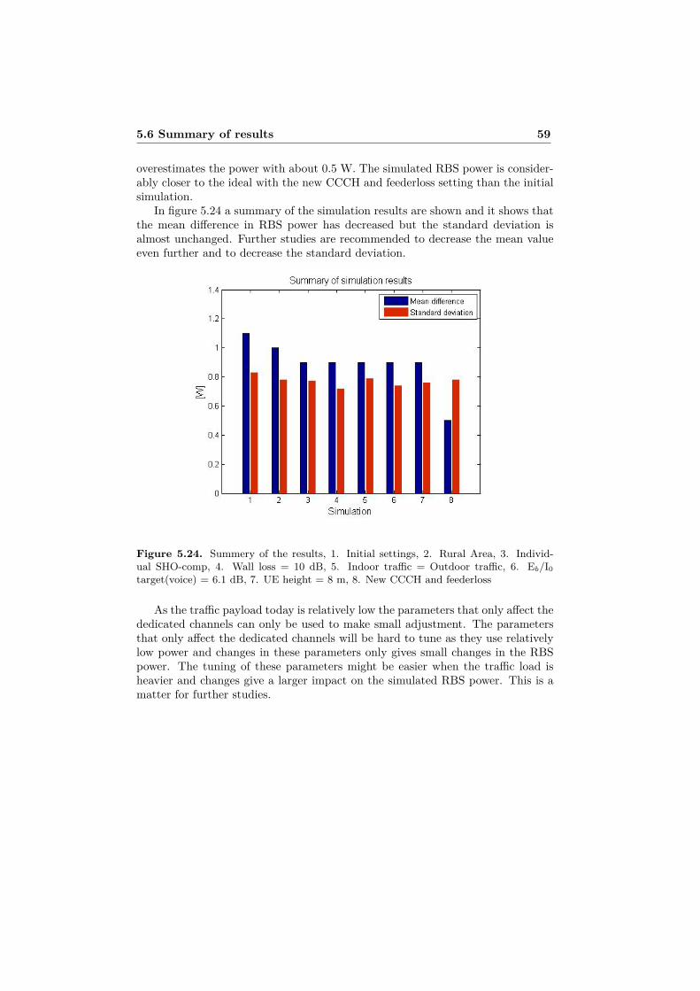
5.6 Summary of results 59
overestimates the power with about 0.5 W. The simulated RBS power is consider-ably closer to the ideal with the new CCCH and feederloss setting than the initialsimulation.
In figure 5.24 a summary of the simulation results are shown and it shows thatthe mean difference in RBS power has decreased but the standard deviation isalmost unchanged. Further studies are recommended to decrease the mean valueeven further and to decrease the standard deviation.
Figure 5.24. Summery of the results, 1. Initial settings, 2. Rural Area, 3. Individ-ual SHO-comp, 4. Wall loss = 10 dB, 5. Indoor traffic = Outdoor traffic, 6. Eb/I0target(voice) = 6.1 dB, 7. UE height = 8 m, 8. New CCCH and feederloss
As the traffic payload today is relatively low the parameters that only affect thededicated channels can only be used to make small adjustment. The parametersthat only affect the dedicated channels will be hard to tune as they use relativelylow power and changes in these parameters only gives small changes in the RBSpower. The tuning of these parameters might be easier when the traffic load isheavier and changes give a larger impact on the simulated RBS power. This is amatter for further studies.
60 Benchmarking of RBS power between simulation result and fielddata

Chapter 6
Other findings
When converting the traffic payload from kbits to Erlang the payload has to bedivided by the SHO-factor to get an accurate number of Erlang. As described insection 3.3.2 the traffic payload is multiplied by a quotient, K in equation 3.6, ofthe SHO-factor from the field statistics and Astrid to get the right amount of trafficinto Astrid. This gives that the traffic payload is first divided and then multipliedby the SHO-factor from the field statistics. Therefore the field statistics SHO-factor calculation is unnecessary and the SHO-factor from reality is not needed inthe traffic payload calculations.
61

62 Other findings
Chapter 7
Conclusion
The assignment for this master thesis was to evaluate and benchmark the simulatorAstrid with real network data. This includes improving the simulation model andevaluating and improving the methods. In particular there were two parts of thisthesis. In addition a benchmark of different Astrid versions was completed, theresult from this study is presented in Appendix A
In the first part of the study simulations were made with even and uneventraffic distribution and the HSDPA bit rates were then compared. As there wasmissing traffic payload data to almost 40% of the cells, further studies are needed toconclude if there is worth the effort of using traffic distribution from field statisticsinstead of evenly distributed traffic.
The second part of the thesis project was to benchmark the simulated RBSpower with the real RBS power to get an accurate power and interference level inthe simulations. Measurement in [11] shows that Rural Area is a better channelmodel then Typical Urban in city centers, the simulations results confirms this.With today’s traffic load the main part of the power used by the RBS is the com-mon control channels (CCCH) and in this simulation project the CCCH was notupdate to the same values as in the real network and therefore causing in aver-age about 0.4 W extra RBS power. With the right CCCH settings the simulatoroverestimates the RBS power with about 0.5 W. As the traffic payload today isrelatively low the parameters that only affect the dedicated channels can only beused to make small adjustment.
63

64 Conclusion

Chapter 8
Further work
The following are recommendations for further studies.
• In this thesis a study of the gain in simulation accuracy when using trafficdistribution from field statistics compared to evenly distributed traffic wascompleted. The simulated network had only field statistics for 60% of thecells. This leads to inaccuracy in the result. Therefore a study of the samekind is recommended to be completed but with a network where there arefield statistics for all cells. The recommended study should conclude if thereis worth the effort of using traffic distribution from field statistics instead ofevenly distributed traffic.
• With today’s traffic load the common control channels use the largest partif the RBS power, hence the dedicated traffic channels use a small part ofthe RBS power. Therefore the parameters that only affect the dedicatedchannels are hard to tune today. Therefore the same kind of study as ischapter 5 is recommended to be completed when the traffic payload hasincreased. The recommended study could work with combinations of theareas discussed in section 5.5 to get the simulated RBS power as close to thereal RBS power as possible.
65

66 Further work
Bibliography
[1] 3GPP. Technical Specification Group Radio Access Network; High SpeedDownlink Packet Access: UE radio transmission and reception, 2002. TR25.890 v 1.0.0.
[2] 3GPP. Technical Specification Group Radio Access Networks; Deploymentaspects, 2002. TR 25.943 v 4.2.0.
[3] C. Bettstetter. GSM Switching Services & Protocols. John Wiley & Sons,2001. ISBN 0-471-49903-X.
[4] Ericsson. WCDMA Evolved, the first step - HSDPA, 2004. White paper.
[5] Ericsson. EB/N0 values for coverage and capacity dimensioning, 2005.133/100 56-HSD 101 02/04 Rev B.
[6] Ericsson. Astrid 1.0: A static Wireless Network Simulator, 2006.
[7] Ericsson. WCDMA Air Interface, 2006. LZU 108 5306 R5C.
[8] H. Holma and A. Toskala. WCDMA for UMTS. John Wiley & Sons, 2001.ISBN 0-471-48687-6.
[9] H. Holma and A. Toskala. HSDPA/HSUPA for UMTS. John Wiley & Sons,2006. ISBN-13 978-0-470-01884-2.
[10] R. Krüger and M. Heeinz. UMTS Introduction and Measurement. Rohde &Schwarz, 2001.
[11] P. Ökvist and K. Larsson. Orthogonality measurement in live 3G networks.Ericsson Confidential, 2007. EAB-06:057211 Uen.
[12] W. Lee. Mobile Cellular Telcommuncations. McGraw-Hill, Inc, 1995. ISBN0-07-113479-4.
[13] T. Ojandperä and R. Prasad. Wideband CDMA for Third Generation MobileCummunications. Artech House, 1998. ISBN 0-89006-735-X.
[14] S. Parkvall; E. Englund; P. Malm; T. Hedberg; M. Persson and J. Peisa.WCDMA evolved highspeed packetdata services. Ericsson Review, (2), 2003.
67
68 Bibliography
[15] Qualcomm CDMA Technologies. HSDPA for improved downlink data trans-fer, 2004. White paper.
[16] A. Simonsson and T. Lundberg. Live Traffic Soft Handover Factors andHandover Rates. Ericsson Confidential, 2006. 1/0363-3/FCP 103 6532 Uen.
[17] J. Zander and K. Seong-Lyun. Radio Resource Management for WirelessNetworks. Artech House Publishers, 2001. ISBN 1-58053-146-6.
Appendix A
Benchmarking of Astridversion 1.0.17
Before starting with the actual thesis work a comparison between Astrid versions1.0.17, 1.0.4 and new is completed. Astrid version 1.0.17 is relatively new versionand the reason for doing this benchmarking is to see if the updates from earlierversions give some changes in the final results. Another reason for doing this isthat I should get used to handle the simulator. Astrid version new was the firstversion of Astrid and therefore the oldest of these three versions. The generalsimulation configuration for these simulations is as follow.
• 5 meter map resolution with 3D building data base
• Realistic network site data (positions, feeder losses, antenna tilts, powersettings. . . )
• Path loss prediction with the Urban propagation model
– Best of Half screen and Micro cell model– The indoor model use 12 dB wall loss and 0.8 dB/m building penetra-
tion slope
• UE antenna height, 1.5 m
• Traffic - HSDPA only
In the figures A.1- A.4 below there are plots from simulations with only HSDPAtraffic in different scenarios. There are simulations with two types of channelmodels, Typical Urban 3 and Pedestrian A.
One thing that differs between version 1.0.17 and the other two versions isthe parameter HS_UEcat, which specifies the UE category in version 1.0.17; seeAppendix G for more information about UE categories. The UE category specifieswhat kind of modulations that can be used. In Astrid versions new and 1.0.4 thereis instead a parameter called HSmod that can be set to QPSK or ’QPSK and
69
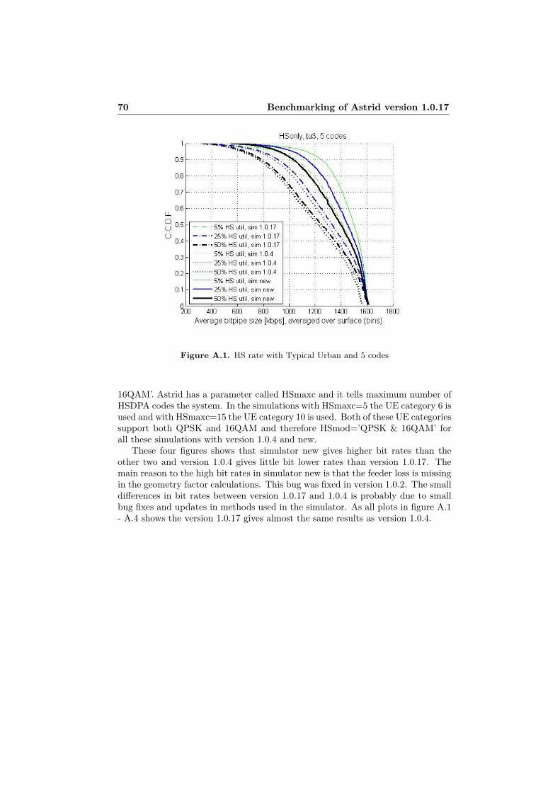
70 Benchmarking of Astrid version 1.0.17
Figure A.1. HS rate with Typical Urban and 5 codes
16QAM’. Astrid has a parameter called HSmaxc and it tells maximum number ofHSDPA codes the system. In the simulations with HSmaxc=5 the UE category 6 isused and with HSmaxc=15 the UE category 10 is used. Both of these UE categoriessupport both QPSK and 16QAM and therefore HSmod=’QPSK & 16QAM’ forall these simulations with version 1.0.4 and new.
These four figures shows that simulator new gives higher bit rates than theother two and version 1.0.4 gives little bit lower rates than version 1.0.17. Themain reason to the high bit rates in simulator new is that the feeder loss is missingin the geometry factor calculations. This bug was fixed in version 1.0.2. The smalldifferences in bit rates between version 1.0.17 and 1.0.4 is probably due to smallbug fixes and updates in methods used in the simulator. As all plots in figure A.1- A.4 shows the version 1.0.17 gives almost the same results as version 1.0.4.

71
Figure A.2. HS rate with Pedestrian A and 5 codes
Figure A.3. HS rate with Typical Urban and 15 codes

72 Benchmarking of Astrid version 1.0.17
Figure A.4. HS rate with Pedestrian A and 15 codes

Appendix B
Astrid parameters
Some of the parameters used in Astrid be explained in the chapter
Astrid parameterssp.simHS Indicating whether HSDPA is simulatedsp.simUL Indicating whether the uplink is simulatedap.dl_ebio_target Sets the Eb/I0 target in the downlink,
(depends on channel model and velocity)sc.serv_channel Sets the channel model used for R99 trafficsc.serv_veloc Sets the velocity of the UEsap.HSutil Variable for the average HSDPA power utilizationap.HSffmap Sets the channel model for HSDPA trafficap.HS_UEcat Sets the UE category for HSDPAap.HSvel Sets the HSDPA user velocityap.HSmaxc Maximum number of codes available in the systemap.sho_maxlinks Maximum number of SHO-linksap.sho_margin Sets SHO windowmp.demand.service Sets the simulated servicesmp.demand.load_factor Describes the distribution
between simulated servicesmp.mix.demands Sets the demanded mix of the trafficmp.mix.scale_factors Sets Erlang per km2
Table B.1. Parameters in Astrid
73

Appendix C
Simulation parametersetting
Parameter settings of the some interesting parameters used in the simulations arepresented in this Appendix.
Parameter settingsp.simHS = 1sp.simUL = 1ap.HSvel = 3.6 km/hmp.mix.demands = [ ], means no R99 traffic
Table C.1. Parameter setting in Appendix A
Parameter settingsp.simHS = 1sp.simUL = 0ap.HSvel = 3.6 km/hmp.demand.service = [1 2 3], means CS 12.2, CS 64 and PS 64mp.demand.load_factor = [0.8784 0.0008 0.1208]mp.mix.demands = [22 23], means indoor and outdoor
Table C.2. Parameter setting in chapter 4
74

75
Parameter settingsp.simHS = 0sp.simUL = 0sc.serv_channel = Typical Urbansc.serv_veloc = 3 km/hap.dl_ebio_target = 7.2 dB, CS 12.2kbpsap.dl_ebio_target = 7.1 dB, CS 64kbpsap.dl_ebio_target = 6.4 dB, PS 64kbpsmp.demand.service = [1 2 3], means CS 12.2, CS 64 and PS 64mp.demand.load_factor = [0.9597 0.0003 0.04]mp.mix.demands = [1 2], means indoor and outdoorThrough wall constant = 12 dBIndoor slope = 0.8 dB/m
Table C.3. Initial parameter setting in chapter 5

Appendix D
Model of Common ControlChannels
The simulated common control channels are the common pilot channel (CPICH),the broadcast channel (BCH), the primary synchronization channel (PSCH) andthe secondary synchronization channel (SSCH). As mention before the CPICHchannel is typically set to 10% of the nominal RBS power and the others CCCHare set relatively to the CPICH. The CPICH channel is used all the time butthe other CCCHs are not. To get a good simulated CCCH, each channel has anactivity factor, α, (this is not only applied to CCCH). In table D.1 the activityfactor used in these simulations for the CCCH is shown.
Channel αCPICH 1BCH 0.9PSCH 0.1SSCH 0.1
Table D.1. Activity factors for CCCH
The total power used by the CCCH is then calculated by using the equationD.1. Where the P denotes power and R is the power relative the CPICH power.
PCCCH = PCPICH · (1 + RB · αB + RP · αP + RS · αS) (D.1)
76

Appendix E
HSDPA utilization
The HSDPA utilization reflects the time the HSDPA channels are in use. Forexample if HSDPA utilization is the used in 3 minutes during an hour the HSDPAutilization is 5%, as figure E.1.
Figure E.1. HSDPA utilization
The HSDPA utilization can also be explained by using the interference. If forexample a UE hears interference from 10 surrounding cells but there is only oneof those that is using HSDPA at the same time as the UE. Then the HSDPAutilization is 10%.
77

Appendix F
Field statistics counter
CounterpmDlTrafficVolumeCs12pmDlTrafficVolumeCs64pmDlTrafficVolumePs64pmDlTrafficVolumePs128pmDlTrafficVolumePs384
Table F.1. Field statistics counter used for traffic payload calculations
CounterpmSumUesWith1Rls1RlInActSetpmSumUesWith1Rls2RlInActSetpmSumUesWith1Rls3RlInActSetpmSumUesWith2Rls2RlInActSetpmSumUesWith2Rls3RlInActSetpmSumUesWith3Rls3RlInActSet
Table F.2. Field statistics counter used for SHO calculations
CounterpmTransmittedCarrierPower
Table F.3. Field statistics counter used for RBS power
78

Appendix G
User Equipment Categories
The HSDPA UE categories available in Astrid version 1.0.17 are presented in tableG.1.
UE category Supported modulation Max codes Max rate5 QPSK & 16QAM 5 36506 QPSK & 16QAM 5 36507 QPSK & 16QAM 10 73008 QPSK & 16QAM 10 73009 QPSK & 16QAM 15 1021610 QPSK & 16QAM 15 1438312 QPSK 5 1825
Table G.1. UE categories
79

Appendix H
Logical, Transport andPhysical Channels
Logical channels define what type of data that is transferred and are classifiedinto two groups, control channels for the transfer of control information and trafficchannels for transfer of user information. The control channels are:
• BCCH - Broadcast Control Channel, a downlink channel for broadcastingsystem control information.
• PCCH - Paging Control Channel, a downlink that transfers paging informa-tion.
• DCCH - Dedicated Control Channel, a channel that transfers dedicated con-trol information between a UE and the RNC.
• CCCH - Common Control Channel, a channel for transmitting control in-formation between the network and UEs.
The traffic channels are:
• DTCH - Dedicated Traffic Channel, a channel dedicated to one UE, for thetransfer of user information.
• CTCH - Common Traffic Channel, a downlink channel for transfer user in-formation to all or a group of specified UEs.
The transport channel defines how and with what characteristics, data is trans-ferred. Transport channels are divided in common channels and dedicated chan-nels, where the common channels can be used by any user at any time and thededicated channel is reserved for a single user. The only dedicated transport chan-nel is the dedicated channel, DCH, which carries all the information intended fora given user. The common transport channels are:
80
81
• BCH - Broadcast Channel, a channel that transmits information specific tothe network or for a given cell.
• FACH - Forward Access Channel, a downlink channel that carries controlinformation to terminals.
• PCH - Paging Channel, a downlink channel that transmits relevant data tothe paging procedure.
• RACH - Random Access Channel, an uplink that carries control informationthe UE, such as request to set up a connection.
• CPCH - Common Packet Channel, an uplink channel that is an extensionto the RACH channel that carries packet-based user data.
• DSCH - Downlink Shared Channel, a channel that carries dedicated userdata and/or control information.
The physical channels define the exact physical characteristics of the radiochannel and they are divided into common channels, dedicated channels and indi-cation channels. The common physical channels are:
• P-CCPCH - Primary Common Control Physical Channel, a channel thatbroadcasts system information.
• SCH - Synchronization Channel, a channel used for synchronization.
• S-CCPCH - Second Common Control Physical Channel, a channel thattransmits idle-mode signaling and control information to UE.
• P-CPICH - Primary Common Pilot Channel, a channel that sends the scram-bling code of the cell.
• PRACH - Physical Random Access Channel, a uplink channel that amongothers carries access requests.
• PDSCH - Physical Downlink Shared Channel, a channel that carries dedi-cated user data and/or control information.
• PCPCH - Physical Common Packet Channel, a channel that is specificallyintended to carry packet data.
The dedicated channels are:
• DPDCH - Dedicated Physical Data Channel, a channel that transmits ded-icated data.
• DPCCH - Dedicated Physical Control Channel, a channel that transmitscontrol signals, such as power control.
• AICH - Acquisition Indication Channel, a channel that acknowledges theRBS has acquired a UE random access attempt.
82 Logical, Transport and Physical Channels
• PICH - Page Indication Channel, a channel that informs a UE if it shouldmonitor the page channel.
• CSICH - CPCH Status Channel, a downlink channel that carries the statusof the CPCH.
• CD/CA-ICH - Collision Detection/Channel Assignment Indicator Channel,a downlink channel that indicate whether the channel assignment is activeor inactive.
In the MAC and RLC layer the logical channels are mapped onto the transportchannels and in the physical layer the transport channels are mapped onto thephysical channels, the mapping is described in [8] and [10]. This is only R99channels, if for example HSDPA technique is applied some additional channels arerequired.

UpphovsrättDetta dokument hålls tillgängligt på Internet — eller dess framtida ersättare —under 25 år från publiceringsdatum under förutsättning att inga extraordinäraomständigheter uppstår.
Tillgång till dokumentet innebär tillstånd för var och en att läsa, ladda ner,skriva ut enstaka kopior för enskilt bruk och att använda det oförändrat för icke-kommersiell forskning och för undervisning. Överföring av upphovsrätten vid ensenare tidpunkt kan inte upphäva detta tillstånd. All annan användning av doku-mentet kräver upphovsmannens medgivande. För att garantera äktheten, säker-heten och tillgängligheten finns det lösningar av teknisk och administrativ art.
Upphovsmannens ideella rätt innefattar rätt att bli nämnd som upphovsmani den omfattning som god sed kräver vid användning av dokumentet på ovan be-skrivna sätt samt skydd mot att dokumentet ändras eller presenteras i sådan formeller i sådant sammanhang som är kränkande för upphovsmannens litterära ellerkonstnärliga anseende eller egenart.
För ytterligare information om Linköping University Electronic Press se för-lagets hemsida http://www.ep.liu.se/
CopyrightThe publishers will keep this document online on the Internet — or its possi-ble replacement — for a period of 25 years from the date of publication barringexceptional circumstances.
The online availability of the document implies a permanent permission foranyone to read, to download, to print out single copies for your own use andto use it unchanged for any non-commercial research and educational purpose.Subsequent transfers of copyright cannot revoke this permission. All other uses ofthe document are conditional on the consent of the copyright owner. The publisherhas taken technical and administrative measures to assure authenticity, securityand accessibility.
According to intellectual property law the author has the right to be men-tioned when his/her work is accessed as described above and to be protectedagainst infringement.
For additional information about the Linköping University Electronic Pressand its procedures for publication and for assurance of document integrity, pleaserefer to its www home page: http://www.ep.liu.se/
c© Lars Näslund