
Informed Search and Exploration - Computer Science · Best-first search Idea: use an evaluation...
48
Informed Search and Exploration Sections 3.5 and 3.6 Ch. 03 – p.1/39
Transcript of Informed Search and Exploration - Computer Science · Best-first search Idea: use an evaluation...

Informed Search and Exploration
Sections 3.5 and 3.6
Ch. 03 – p.1/39
Outline
Best-first search
A∗ search
Heuristics, pattern databases
IDA∗ search
RBFS search
MA∗ and SMA∗ search
References:The slides were adapted to the 3rd edition ofRussell and Norvig’s textbook using the slides for the 2nd
edition. The example with the inconsistent heuristic wastaken from Dana Nau’s CMSC 421 slides on the samechapter (February 2, 2010 version.)
Ch. 03 – p.2/39
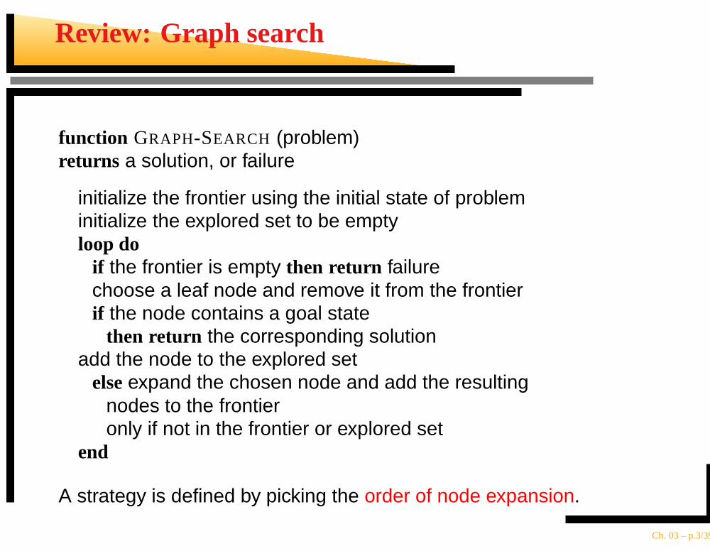
Review: Graph search
function GRAPH-SEARCH (problem)returns a solution, or failure
initialize the frontier using the initial state of probleminitialize the explored set to be emptyloop do
if the frontier is empty then return failurechoose a leaf node and remove it from the frontierif the node contains a goal state
then return the corresponding solutionadd the node to the explored set
elseexpand the chosen node and add the resultingnodes to the frontieronly if not in the frontier or explored set
end
A strategy is defined by picking the order of node expansion.
Ch. 03 – p.3/39
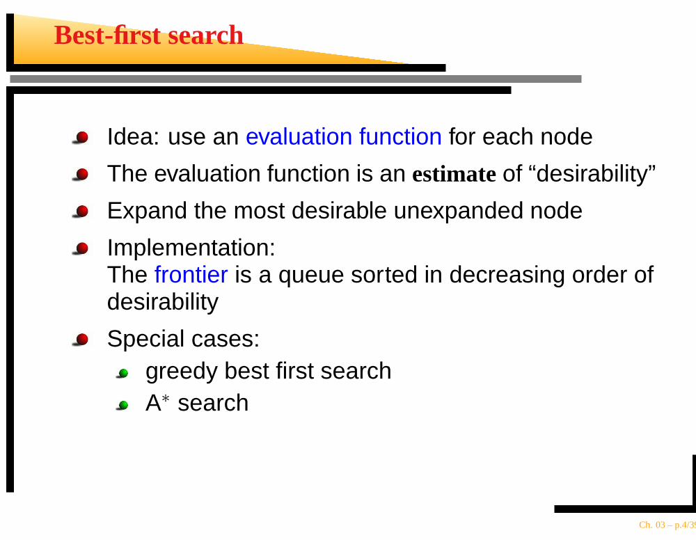
Best-first search
Idea: use an evaluation function for each node
The evaluation function is an estimateof “desirability”
Expand the most desirable unexpanded node
Implementation:The frontier is a queue sorted in decreasing order ofdesirability
Special cases:greedy best first searchA∗ search
Ch. 03 – p.4/39
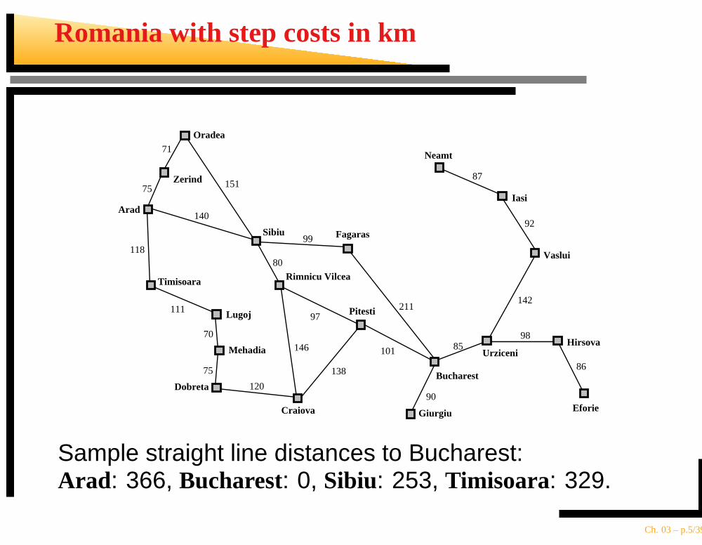
Romania with step costs in km
Giurgiu
UrziceniHirsova
Eforie
Neamt
Oradea
Zerind
Arad
Timisoara
Lugoj
Mehadia
Dobreta
Craiova
Sibiu Fagaras
Pitesti
Vaslui
Iasi
Rimnicu Vilcea
Bucharest
71
75
118
111
70
75
120
151
140
99
80
97
101
211
138
146 85
90
98
142
92
87
86
Sample straight line distances to Bucharest:Arad : 366, Bucharest: 0, Sibiu: 253, Timisoara: 329.
Ch. 03 – p.5/39
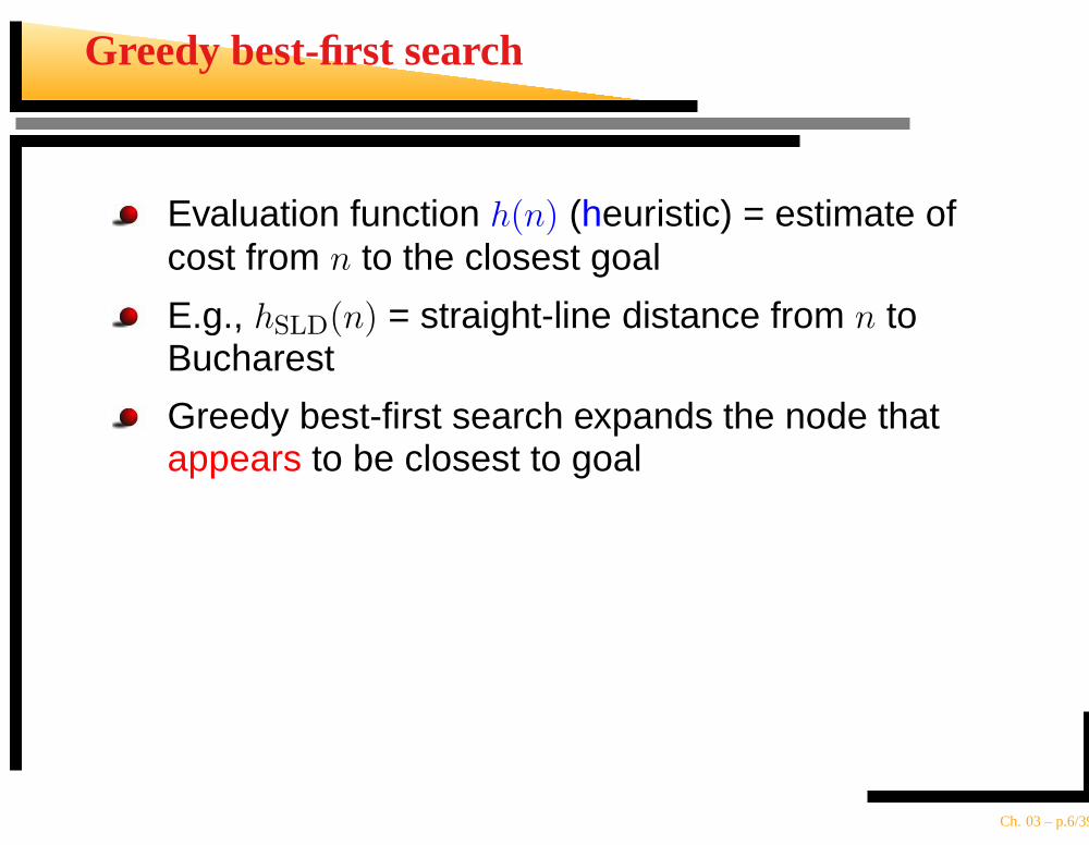
Greedy best-first search
Evaluation function h(n) (heuristic) = estimate ofcost from n to the closest goal
E.g., hSLD(n) = straight-line distance from n toBucharest
Greedy best-first search expands the node thatappears to be closest to goal
Ch. 03 – p.6/39
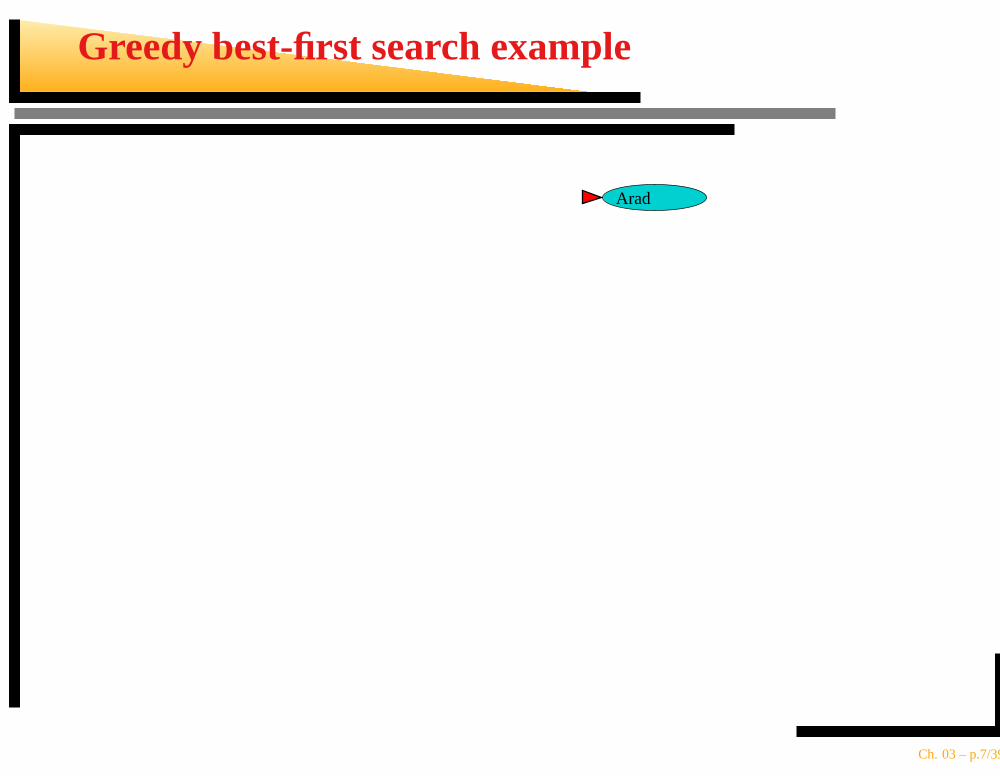
Greedy best-first search example
Arad
Ch. 03 – p.7/39
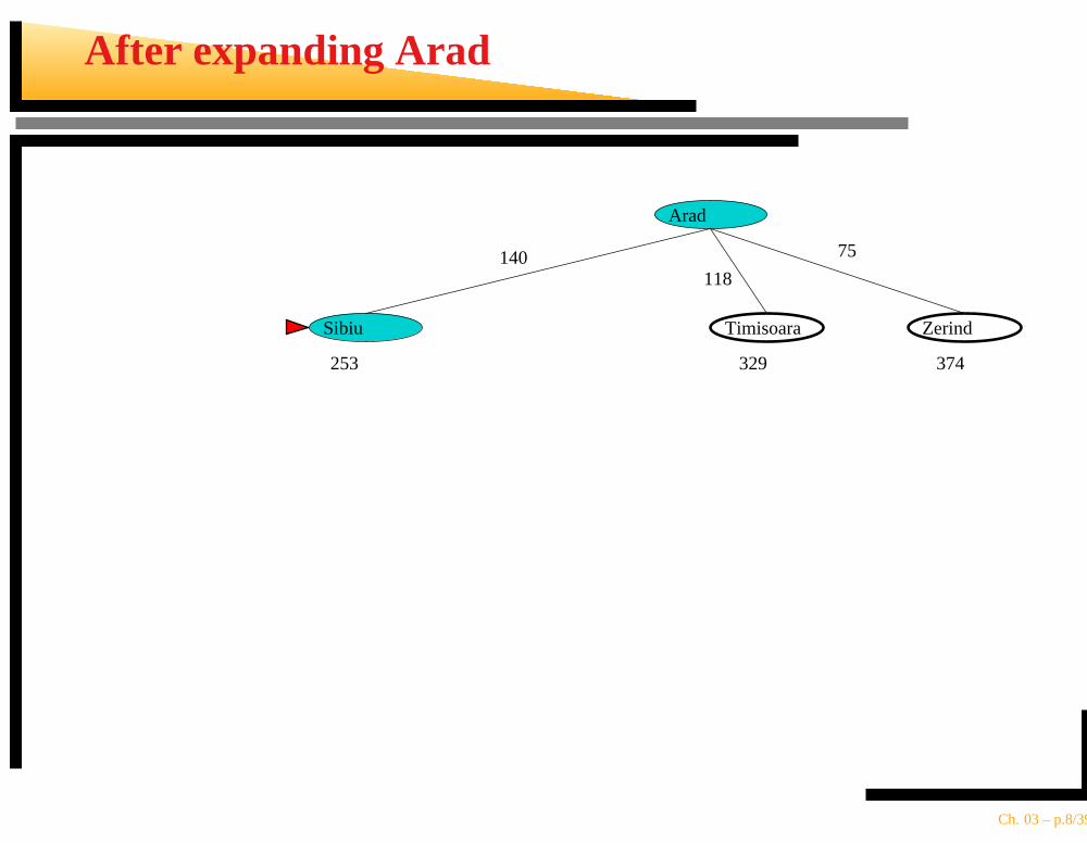
After expanding Arad
374
Sibiu Timisoara
Arad
Zerind
140 75
118
329253
Ch. 03 – p.8/39
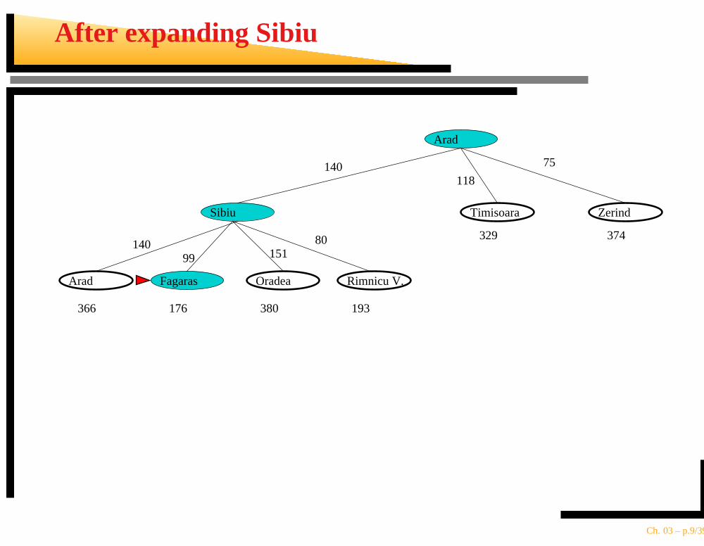
After expanding Sibiu
366 380 193
329 374
Arad Fagaras Oradea Rimnicu V.
Sibiu Timisoara
Arad
Zerind
140
140
75
118
8015199
176
Ch. 03 – p.9/39
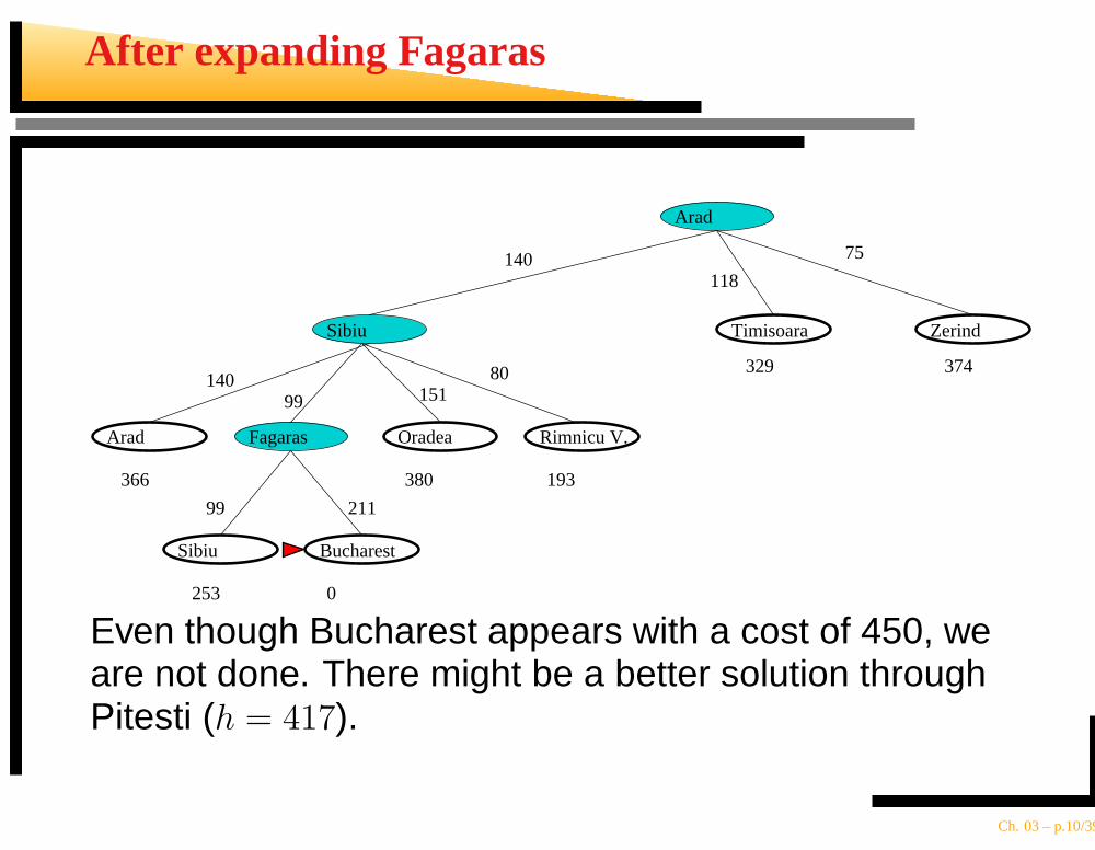
After expanding Fagaras
Bucharest
366 380 193
253 0
329 374
Arad
Sibiu
Fagaras Oradea Rimnicu V.
Sibiu Timisoara
Arad
Zerind
140
140
75
118
21199
8015199
Even though Bucharest appears with a cost of 450, weare not done. There might be a better solution throughPitesti (h = 417).
Ch. 03 – p.10/39
Properties of greedy best-first search
Complete No — can get stuck in loopsFor example, going from Iasi to Fagaras,Iasi→ Neamt→ Iasi→ Neamt→ . . .Complete in finite space with repeated-statechecking
Time O(bm), but a good heuristic can give dramaticimprovement (more later)
Space O(bm)—keeps all nodes in memory
Optimal No(For example, the cost of the path found in theprevious slide was 450. The path Arad, Sibiu,Rimnicu Vilcea, Pitesti, Bucharest has a cost of140+80+97+101 = 418.)
Ch. 03 – p.11/39
A∗ search
Idea: avoid expanding paths that are alreadyexpensive
Evaluation function f(n) = g(n) + h(n)
g(n) = exact cost so far to reach n
h(n) = estimated cost to goal from n
f(n) = estimated total cost of path through n togoal
A∗ search uses an admissible heuristici.e., h(n) ≤ h∗(n) where h∗(n) is the true cost from n.(Also require h(n) ≥ 0, so h(G) = 0 for any goal G.)
Straight line distance (hSLD(n)) is an admissibleheuristic because never overestimates the actualroad distance. Ch. 03 – p.12/39
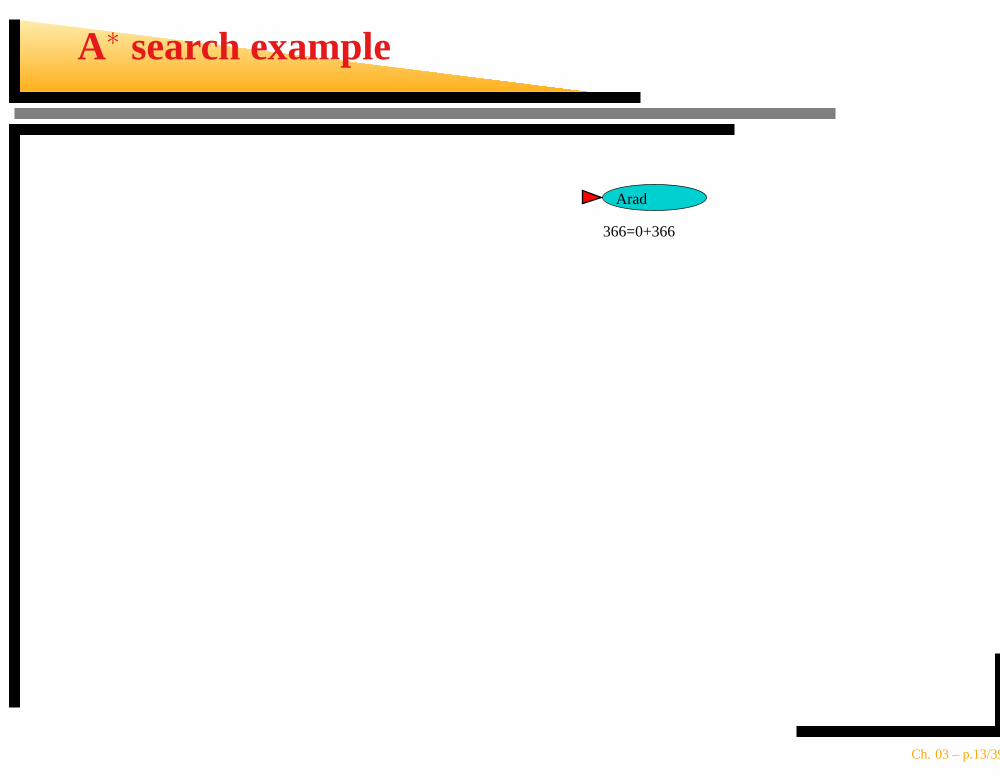
A∗ search example
Arad
366=0+366
Ch. 03 – p.13/39
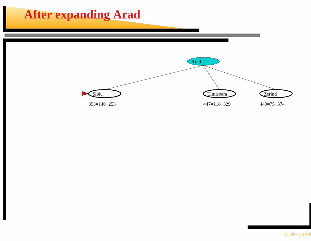
After expanding Arad
Sibiu Timisoara
Arad
Zerind
447=118+329 449=75+374393=140+253
Ch. 03 – p.14/39
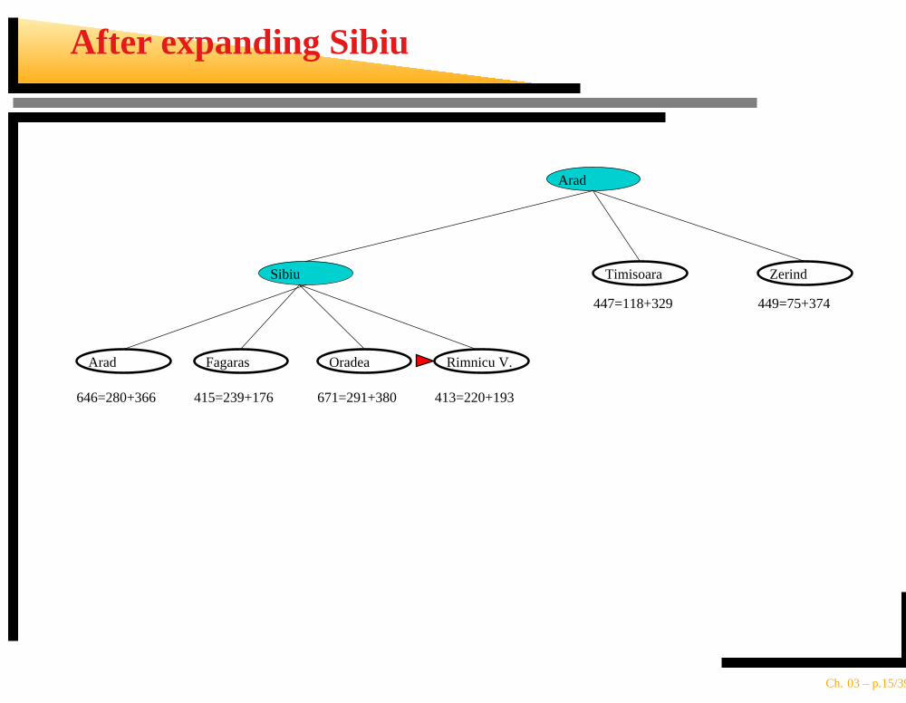
After expanding Sibiu
Arad Fagaras Oradea
Sibiu Timisoara
Arad
Zerind
646=280+366 671=291+380
447=118+329 449=75+374
415=239+176
Rimnicu V.
413=220+193
Ch. 03 – p.15/39
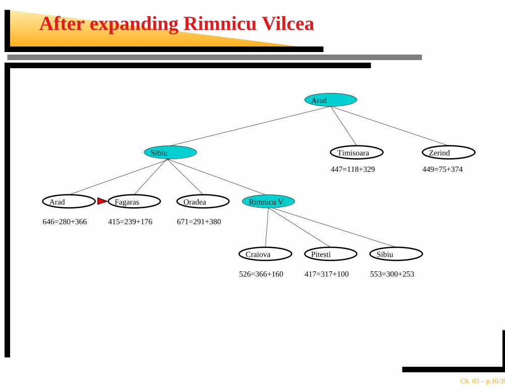
After expanding Rimnicu Vilcea
Arad Fagaras Oradea Rimnicu V.
Sibiu Timisoara
Arad
Zerind
Craiova Pitesti Sibiu
646=280+366 671=291+380
526=366+160 553=300+253
447=118+329 449=75+374
417=317+100
415=239+176
Ch. 03 – p.16/39
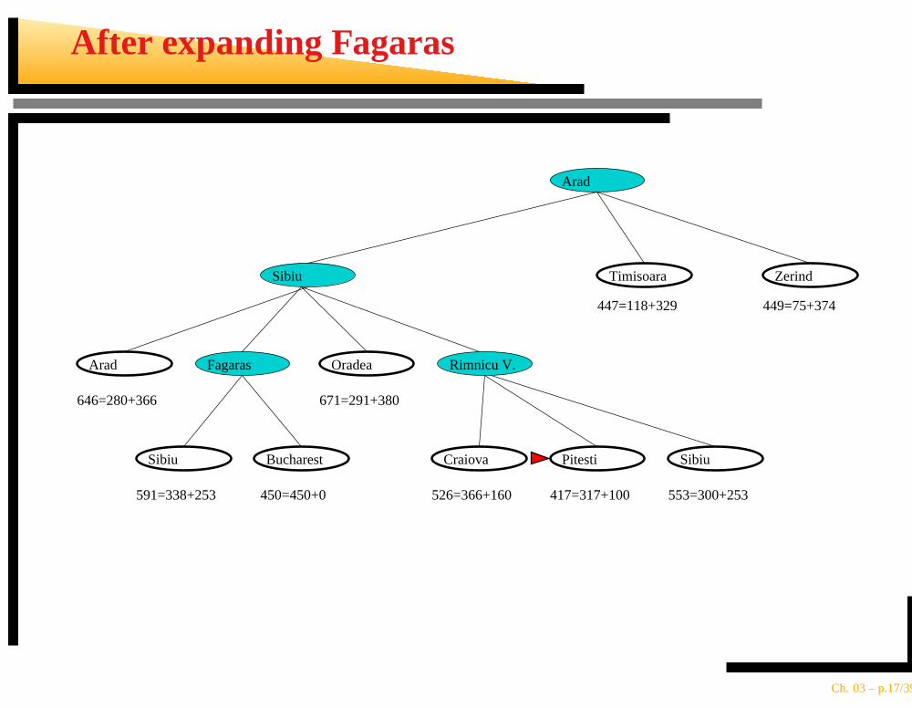
After expanding Fagaras
Bucharest
Arad
Sibiu
Fagaras Oradea Rimnicu V.
Sibiu Timisoara
Arad
Zerind
Craiova Pitesti Sibiu
646=280+366
591=338+253 450=450+0
671=291+380
526=366+160 553=300+253
447=118+329 449=75+374
417=317+100
Ch. 03 – p.17/39
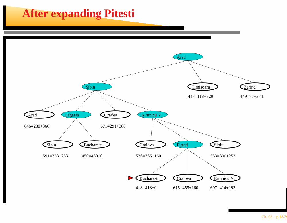
After expanding Pitesti
Bucharest
Bucharest
Arad
Sibiu
Fagaras Oradea Rimnicu V.
Sibiu Timisoara
Arad
Zerind
Craiova Pitesti Sibiu
Rimnicu V.Craiova
646=280+366
591=338+253 450=450+0
671=291+380
526=366+160 553=300+253
418=418+0 615=455+160 607=414+193
447=118+329 449=75+374
Ch. 03 – p.18/39
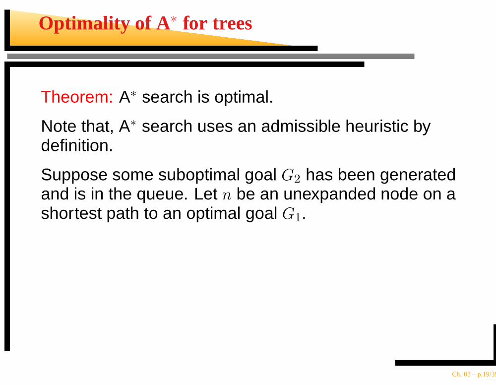
Optimality of A ∗ for trees
Theorem: A∗ search is optimal.
Note that, A∗ search uses an admissible heuristic bydefinition.
Suppose some suboptimal goal G2 has been generatedand is in the queue. Let n be an unexpanded node on ashortest path to an optimal goal G1.
Ch. 03 – p.19/39
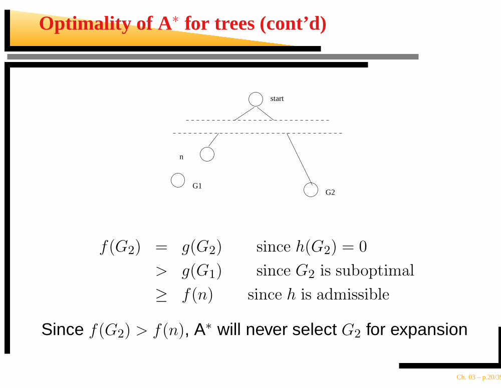
Optimality of A ∗ for trees (cont’d)
n
G1G2
start
f(G2) = g(G2) since h(G2) = 0
> g(G1) since G2 is suboptimal
≥ f(n) since h is admissible
Since f(G2) > f(n), A∗ will never select G2 for expansion
Ch. 03 – p.20/39
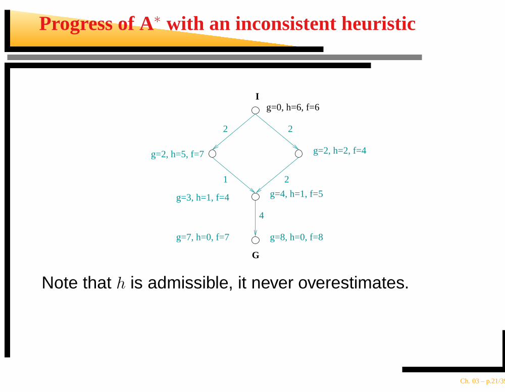
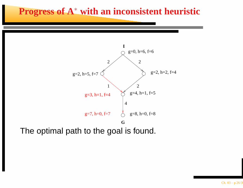
Progress of A∗ with an inconsistent heuristic
2 2
1 2
4
g=0, h=6, f=6
g=3, h=1, f=4
g=2, h=5, f=7 g=2, h=2, f=4
g=4, h=1, f=5
g=8, h=0, f=8
I
G
g=7, h=0, f=7
Note that h is admissible, it never overestimates.
Ch. 03 – p.21/39
Progress of A∗ with an inconsistent heuristic
2 2
1 2
4
g=0, h=6, f=6
g=3, h=1, f=4
g=2, h=5, f=7 g=2, h=2, f=4
g=4, h=1, f=5
g=8, h=0, f=8
I
G
g=7, h=0, f=7
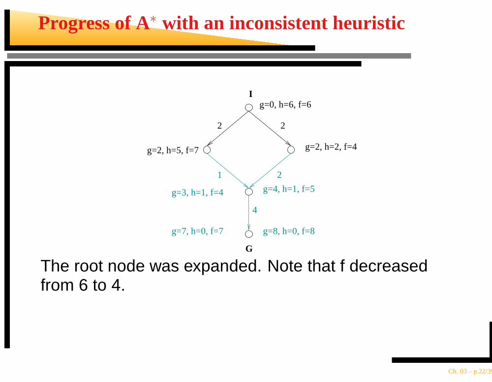
The root node was expanded. Note that f decreasedfrom 6 to 4.
Ch. 03 – p.22/39
Progress of A∗ with an inconsistent heuristic
2 2
1 2
4
g=0, h=6, f=6
g=3, h=1, f=4
g=2, h=5, f=7 g=2, h=2, f=4
g=4, h=1, f=5
g=8, h=0, f=8
I
G
g=7, h=0, f=7
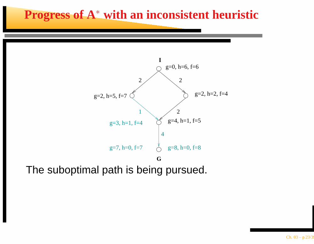
The suboptimal path is being pursued.
Ch. 03 – p.23/39
Progress of A∗ with an inconsistent heuristic
2 2
1 2
4
g=0, h=6, f=6
g=3, h=1, f=4
g=2, h=5, f=7 g=2, h=2, f=4
g=4, h=1, f=5
g=8, h=0, f=8
I
G
g=7, h=0, f=7
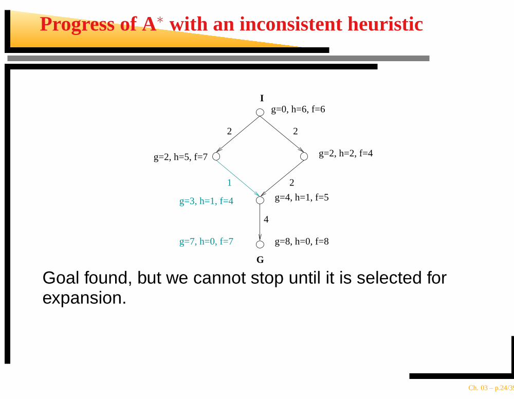
Goal found, but we cannot stop until it is selected forexpansion.
Ch. 03 – p.24/39
Progress of A∗ with an inconsistent heuristic
2 2
1 2
4
g=0, h=6, f=6
g=3, h=1, f=4
g=2, h=5, f=7 g=2, h=2, f=4
g=4, h=1, f=5
g=8, h=0, f=8
I
G
g=7, h=0, f=7
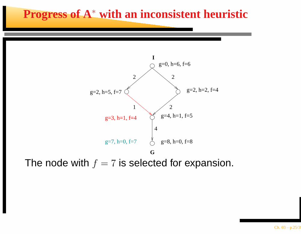
The node with f = 7 is selected for expansion.
Ch. 03 – p.25/39
Progress of A∗ with an inconsistent heuristic
2 2
1 2
4
g=0, h=6, f=6
g=3, h=1, f=4
g=2, h=5, f=7 g=2, h=2, f=4
g=4, h=1, f=5
g=8, h=0, f=8
I
G
g=7, h=0, f=7
The optimal path to the goal is found.
Ch. 03 – p.26/39
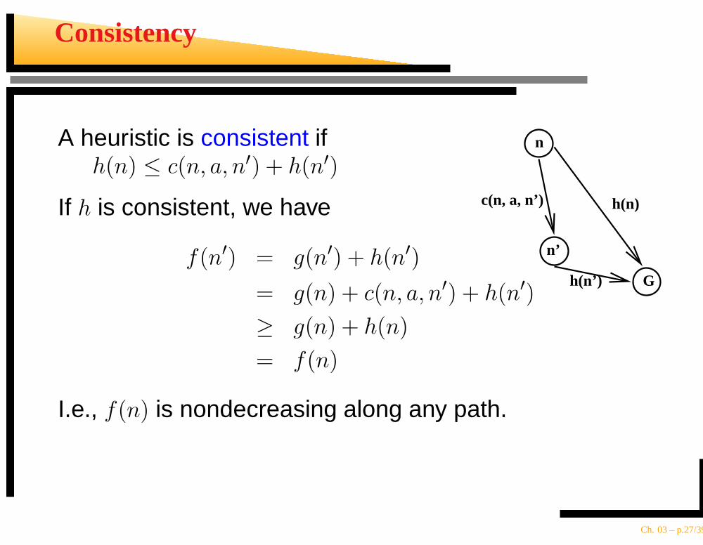
Consistency
A heuristic is consistent if
n’
n
G
h(n)
h(n’)
c(n, a, n’)
h(n) ≤ c(n, a, n′) + h(n′)
If h is consistent, we have
f(n′) = g(n′) + h(n′)
= g(n) + c(n, a, n′) + h(n′)
≥ g(n) + h(n)
= f(n)
I.e., f(n) is nondecreasing along any path.
Ch. 03 – p.27/39
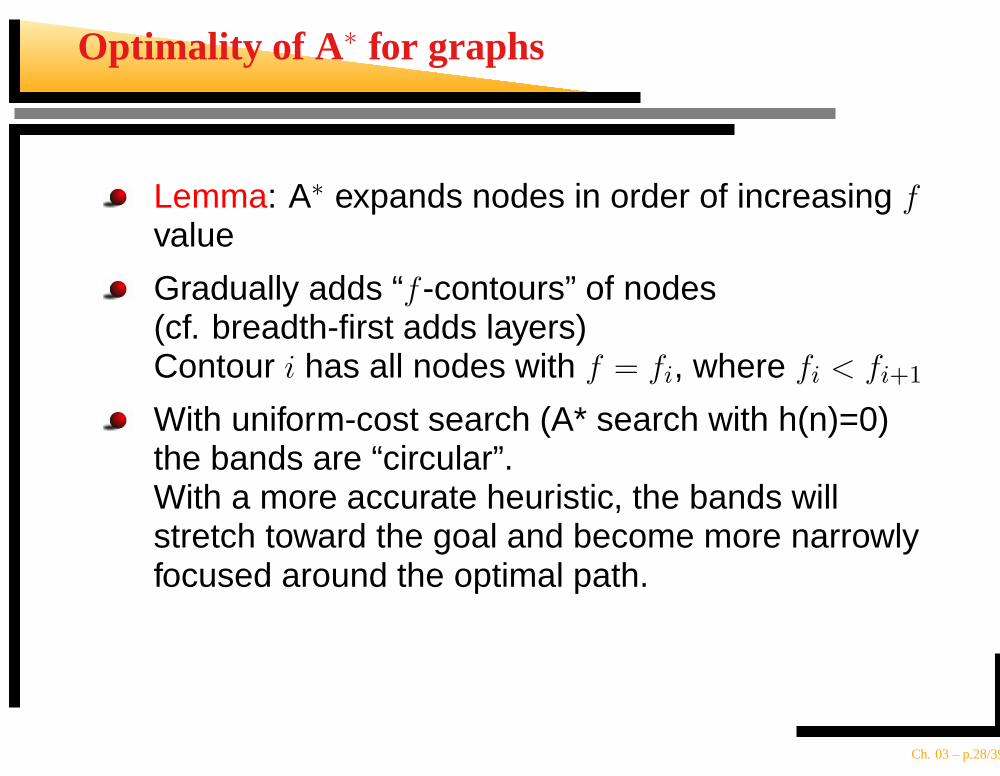
Optimality of A ∗ for graphs
Lemma: A∗ expands nodes in order of increasing fvalue
Gradually adds “f -contours” of nodes(cf. breadth-first adds layers)Contour i has all nodes with f = fi, where fi < fi+1
With uniform-cost search (A* search with h(n)=0)the bands are “circular”.With a more accurate heuristic, the bands willstretch toward the goal and become more narrowlyfocused around the optimal path.
Ch. 03 – p.28/39
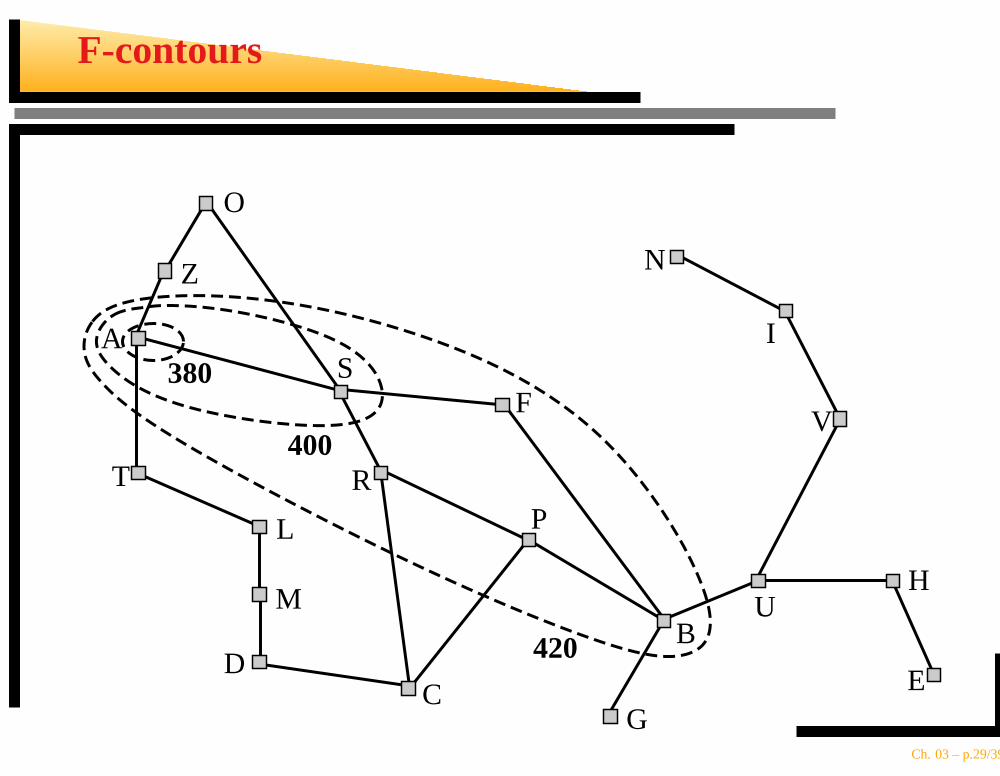
F-contours
O
Z
A
T
L
M
DC
R
F
P
G
BU
H
E
V
I
N
380
400
420
S
Ch. 03 – p.29/39
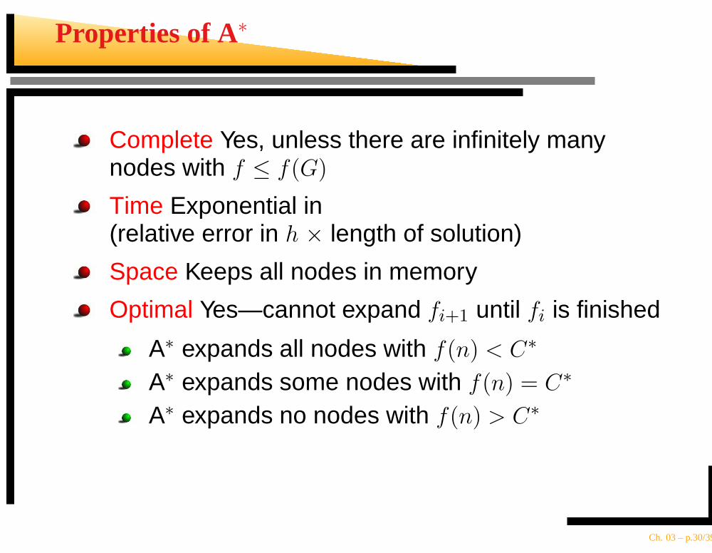
Properties of A∗
Complete Yes, unless there are infinitely manynodes with f ≤ f(G)
Time Exponential in(relative error in h × length of solution)
Space Keeps all nodes in memory
Optimal Yes—cannot expand fi+1 until fi is finished
A∗ expands all nodes with f(n) < C∗
A∗ expands some nodes with f(n) = C∗
A∗ expands no nodes with f(n) > C∗
Ch. 03 – p.30/39
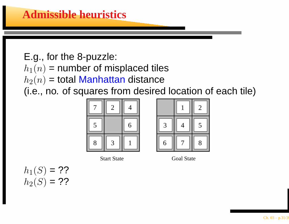
Admissible heuristics
E.g., for the 8-puzzle:h1(n) = number of misplaced tilesh2(n) = total Manhattan distance(i.e., no. of squares from desired location of each tile)
2
Start State Goal State
1
3 4
6 7
5
1
2
3
4
6
7
8
5
8
h1(S) = ??h2(S) = ??
Ch. 03 – p.31/39
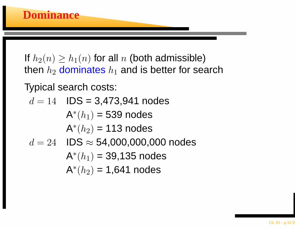
Dominance
If h2(n) ≥ h1(n) for all n (both admissible)then h2 dominates h1 and is better for search
Typical search costs:d = 14 IDS = 3,473,941 nodes
A∗(h1) = 539 nodesA∗(h2) = 113 nodes
d = 24 IDS ≈ 54,000,000,000 nodesA∗(h1) = 39,135 nodesA∗(h2) = 1,641 nodes
Ch. 03 – p.32/39
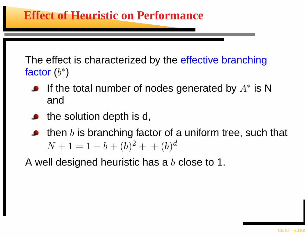
Effect of Heuristic on Performance
The effect is characterized by the effective branchingfactor (b∗)
If the total number of nodes generated by A∗ is Nand
the solution depth is d,
then b is branching factor of a uniform tree, such thatN + 1 = 1 + b + (b)2 + + (b)d
A well designed heuristic has a b close to 1.
Ch. 03 – p.33/39
Relaxed problems
Admissible heuristics can be derived from the exactsolution cost of a relaxed version of the problem
If the rules of the 8-puzzle are relaxed so that a tilecan move anywhere, then h1(n) gives the shortestsolution
If the rules are relaxed so that a tile can move to anyadjacent square, then h2(n) gives the shortestsolution
Key point: the optimal solution cost of a relaxedproblem is no greater than the optimal solution costof the real problem
Ch. 03 – p.34/39
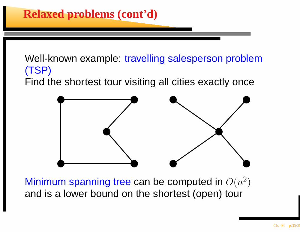
Relaxed problems (cont’d)
Well-known example: travelling salesperson problem(TSP)Find the shortest tour visiting all cities exactly once
Minimum spanning tree can be computed in O(n2)and is a lower bound on the shortest (open) tour
Ch. 03 – p.35/39
Pattern databases
Admissible heuristics can also be generated fromthe solution cost of sub- problems.
For example, in the 8-puzzle problem a sub-problemof getting the tiles 2, 4, 6, and 8 into position is alower bound on solving the complete problem.
Pattern databases store the solution costs for all thesub-problem instances.
The choice of sub-problem is flexible:for the 8-puzzle a subproblem for 2,4,6,8 or 1,2,3,4or 5,6,7,8, . . . could be created.
Ch. 03 – p.36/39
Performance of A∗
The absolute error of a heuristic is defined as∆ ≡ h∗ − h
The relative error of a heuristic is defined asǫ ≡ h
∗
−h
h∗
Complexity with constant step costs: O(bǫd)
Problem: there can be exponentially many stateswith f(n) < C∗ even if the absolute error is boundedby a constant
Ch. 03 – p.37/39
Iterative Deepening A* (IDA*)
Idea: perform iterations of DFS. The cutoff is definedbased on the f -cost rather than the depth of a node.
Each iteration expands all nodes inside the contourfor the current f -cost, peeping over the contour tofind out where the contour lies.
Ch. 03 – p.38/39
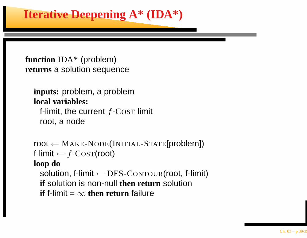
Iterative Deepening A* (IDA*)
function IDA* (problem)returns a solution sequence
inputs: problem, a problemlocal variables:
f-limit, the current f -COST limitroot, a node
root← MAKE-NODE(INITIAL -STATE[problem])f-limit← f -COST(root)loop do
solution, f-limit← DFS-CONTOUR(root, f-limit)if solution is non-null then return solutionif f-limit =∞ then return failure
Ch. 03 – p.39/39
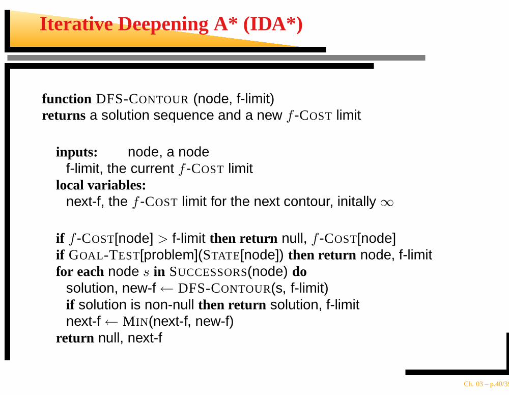
Iterative Deepening A* (IDA*)
function DFS-CONTOUR (node, f-limit)returns a solution sequence and a new f -COST limit
inputs: node, a nodef-limit, the current f -COST limit
local variables:next-f, the f -COST limit for the next contour, initally∞
if f -COST[node] > f-limit then return null, f -COST[node]if GOAL-TEST[problem](STATE[node]) then return node, f-limitfor each node s in SUCCESSORS(node) do
solution, new-f← DFS-CONTOUR(s, f-limit)if solution is non-null then return solution, f-limitnext-f← M IN(next-f, new-f)
return null, next-f
Ch. 03 – p.40/39
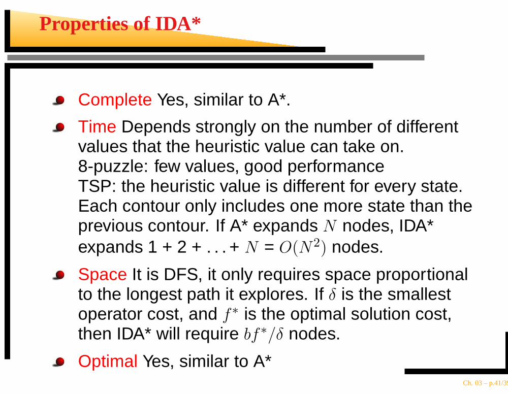
Properties of IDA*
Complete Yes, similar to A*.
Time Depends strongly on the number of differentvalues that the heuristic value can take on.8-puzzle: few values, good performanceTSP: the heuristic value is different for every state.Each contour only includes one more state than theprevious contour. If A* expands N nodes, IDA*expands 1 + 2 + . . . + N = O(N2) nodes.
Space It is DFS, it only requires space proportionalto the longest path it explores. If δ is the smallestoperator cost, and f∗ is the optimal solution cost,then IDA* will require bf∗/δ nodes.
Optimal Yes, similar to A*Ch. 03 – p.41/39
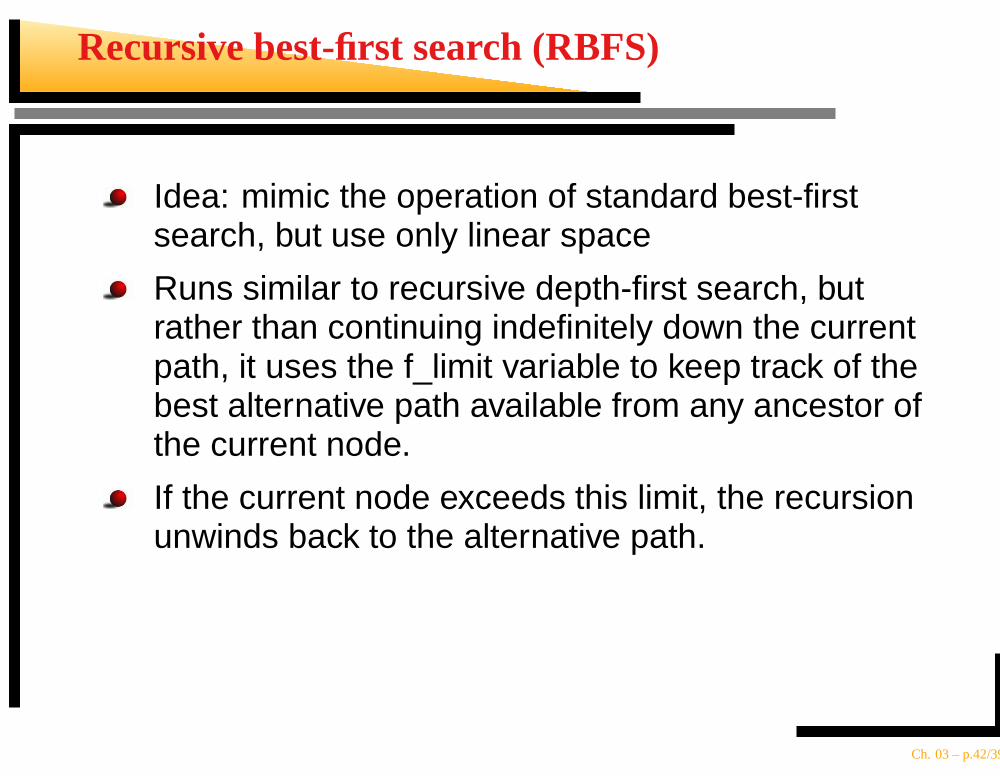
Recursive best-first search (RBFS)
Idea: mimic the operation of standard best-firstsearch, but use only linear space
Runs similar to recursive depth-first search, butrather than continuing indefinitely down the currentpath, it uses the f_limit variable to keep track of thebest alternative path available from any ancestor ofthe current node.
If the current node exceeds this limit, the recursionunwinds back to the alternative path.
Ch. 03 – p.42/39
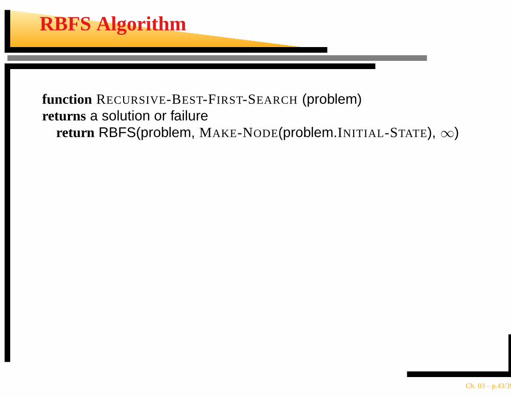
RBFS Algorithm
function RECURSIVE-BEST-FIRST-SEARCH (problem)returns a solution or failure
return RBFS(problem, MAKE-NODE(problem.INITIAL -STATE), ∞)
Ch. 03 – p.43/39
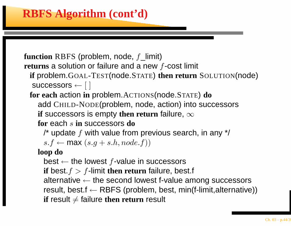
RBFS Algorithm (cont’d)
function RBFS(problem, node, f_limit)returns a solution or failure and a new f -cost limit
if problem.GOAL-TEST(node.STATE) then return SOLUTION(node)successors← [ ]
for each action in problem.ACTIONS(node.STATE) doadd CHILD -NODE(problem, node, action) into successorsif successors is empty then return failure,∞for each s in successors do
/* update f with value from previous search, in any */s.f ← max (s.g + s.h, node.f))
loop dobest← the lowest f -value in successorsif best.f > f -limit then return failure, best.falternative← the second lowest f-value among successorsresult, best.f← RBFS (problem, best, min(f-limit,alternative))if result 6= failure then return result
Ch. 03 – p.44/39
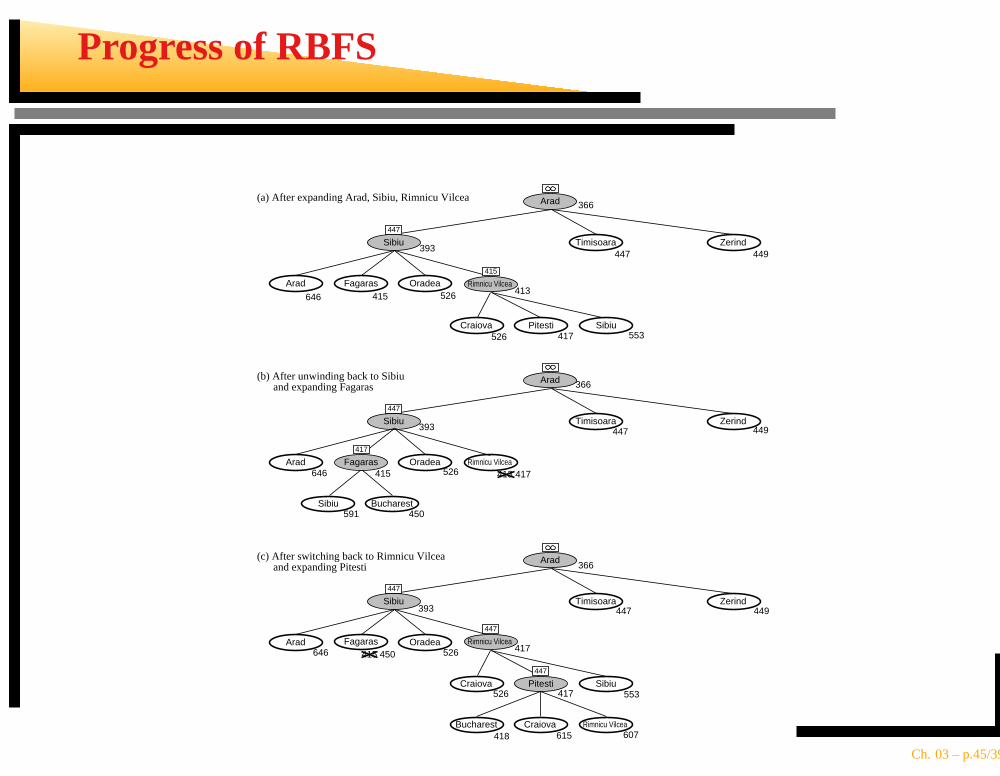
Progress of RBFS
Zerind
Arad
Sibiu
Arad
Timisoara
Fagaras Oradea
Craiova Pitesti Sibiu
Bucharest Craiova Rimnicu Vilcea
Zerind
Arad
Sibiu
Arad
Timisoara
Sibiu Bucharest
Rimnicu VilceaOradea
Zerind
Arad
Sibiu
Arad
Timisoara
Fagaras Oradea Rimnicu Vilcea
Craiova Pitesti Sibiu
646 415 526
526 417 553
646 526
450591
646 526
526 553
418 615 607
447 449
447
447 449
449
366
393
366
393
413
413 417415
366
393
415 450417
417
Rimnicu Vilcea
Fagaras
447
415
447
447
417
(a) After expanding Arad, Sibiu, Rimnicu Vilcea
(c) After switching back to Rimnicu Vilcea and expanding Pitesti
(b) After unwinding back to Sibiu and expanding Fagaras
447
447
Ch. 03 – p.45/39

MA* and SMA*
Idea: use all the available memoryIDA* remembers only the current f -cost limitRBFS uses linear space
Proceeds just like A*, expanding the best leaf untilthe memory is full. When the memory if full, drop theworst leaf node.
Ch. 03 – p.46/39
Summary
The evaluation function for a node n is:f(n) = g(n) + h(n)
If only g(n) is used, we get uniform-cost search
If only h(n) is used, we get greedy best-first search
If both g(n) and h(n) are used with an admissible(and consistent) search we get A∗ search
Ch. 03 – p.47/39
Summary (cont’d)
Admissibility is required to guarantee solutionoptimality for tree search
Consistency is required to guarantee solutionoptimality for graph search
Heuristic search usually brings dramaticimprovement over uninformed search
Keep in mind that the f-contours might still containan exponential number of nodes
Ch. 03 – p.48/39


![BioResource Now - SHIGENshigen.nig.ac.jp/shigen/news/n_letter/2016/nl201610En.pdf · function> get extension from store]. Search for LastPass on the Microsoft store and install it](https://static.fdocument.pub/doc/165x107/5ed3b437a74f540d6d3545ae/bioresource-now-function-get-extension-from-store-search-for-lastpass-on.jpg)