In the Name of God

Morteza Bahram

•Department of Chemistry, Faculty of Science, Urmia University, Urmia, Iran

m.bahram@urmia.ac.ir morteza.bahram@gmail.com

دانشگاه اروميه

Modeling Multi-Way Data with Linearly Dependent Modeling Multi-Way Data with Linearly Dependent

LoadingsLoadings

PARALINDPARALIND

1 .Introduction

Many methods have been proposed for multivariate curve resolution and more

generally for factor or component modeling of (multi-way) data ,

1) Tucker

2) PARAFAC

3) Positive matrix factorization (PMF)

4) MCR-ALS

5) ….

With three-way data, it becomes possible for patterns generated by the

underlying sources of variation to have independent effects in two modes, independent effects in two modes,

yet nonetheless be linearly dependent in a third modeyet nonetheless be linearly dependent in a third mode.

When such linear dependencies exist in the latent factor structure, the most

appropriate PARAFAC solution would show the same dependencies in the

recovered factors.

This solution could be called rank deficient in the sense that the component

matrices for one – or even several – modes would have less than full column

rank. However, the obtained PARAFAC solution will never have this property

because noise causes the estimated loadings for collinear factors to become

linearly independent (though usually they are still quite correlated).

Kiers and Smilde rigorously proved that the uniqueness of

PARAFAC does not hold in cases with collinear factors.

For example, linear dependences could arise when two or more

fluorophores at fixed ratios are present throughout a series of

experiments. Linear dependences also could occur in spectra

modes because of certain types of fluorescence energy transfer

from one type of fluorophore to another one

As stated by Bro if a three-mode array is modeled by

uninformed PARAFAC and if two factors have collinear

profiles in only one mode, the two factors cannot be

uniquely determined in other two modes; if two factors

have collinear profiles in two modes, the two factors will

become undistinguishable and will collapse to a single

factor.

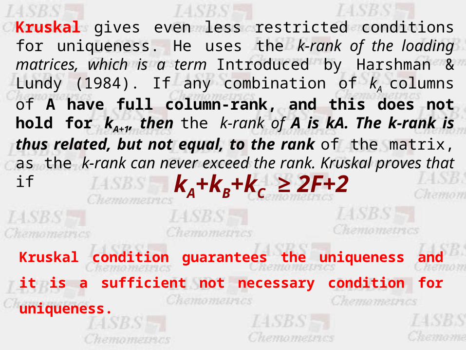
Kruskal gives even less restricted conditions for uniqueness. He uses the k-rank of the loading matrices, which is a term Introduced by Harshman & Lundy (1984). If any combination of kA columns of A have full column-rank, and this does not hold for kA+1, then the k-rank of A is kA. The k-rank is thus related, but not equal, to the rank of the matrix, as the k-rank can never exceed the rank. Kruskal proves that if

kA+kB+kC ≥ 2F+2

Kruskal condition guarantees the uniqueness and it is a

sufficient not necessary condition for uniqueness.

AA

1) Fluorescence excitation-emission matrices (EEMs) with correlated concentration of component .

2) pH – Spectrophotometric data in different concentrations

3) Flow Injection analysis Data

4) GC-MS data with linear dependency

5) Standard addition three–way data

6) etc.

Which data are subjected to be analyzed Which data are subjected to be analyzed by PARALIND?by PARALIND?

HAA-HBB-HCC-HAA-HBB-HCC-

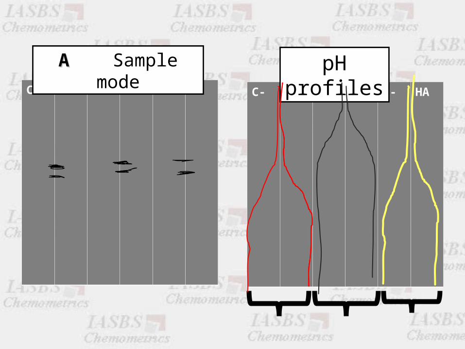
AA Sample mode pH profiles

=C

HAA-HBB-HCC-

A Sample mode

=

HAHBHC 111100000000

000011110000

000000001111

HHAA__

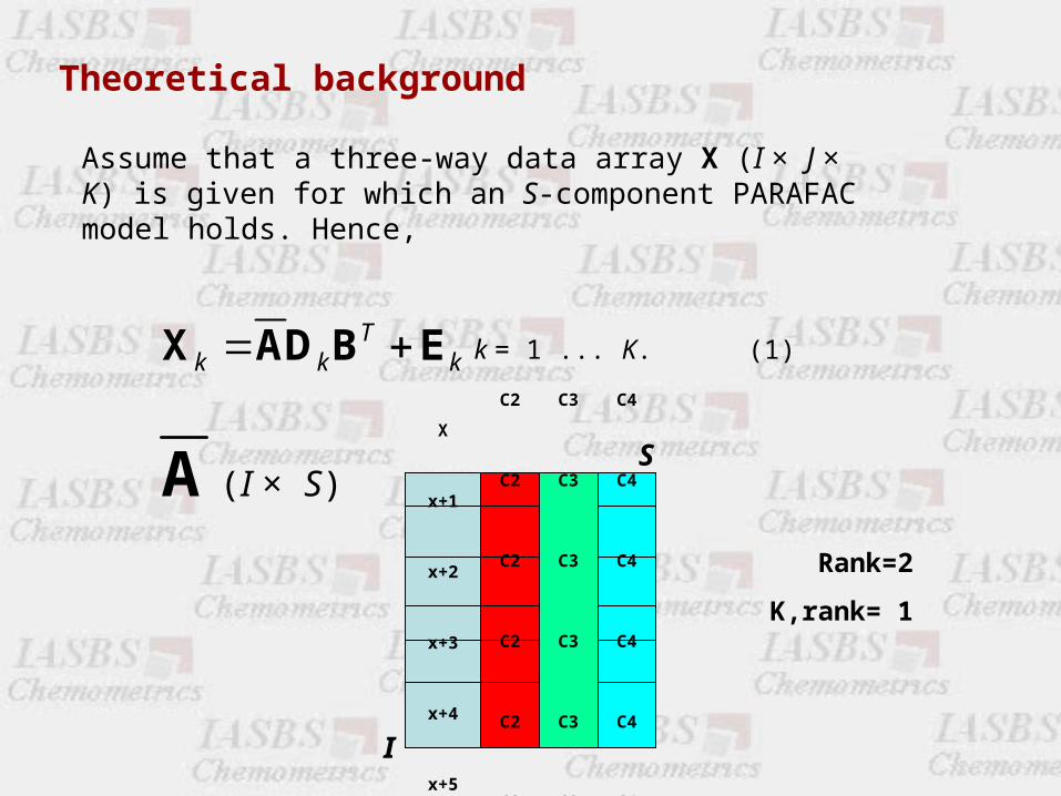
Theoretical background

Assume that a three-way data array X (I × J × K) is given for which an S-component PARAFAC model holds. Hence,

Tk k k X AD B E k = 1 ... K. (1)

A ( I × S)

X

x+1

x+2

x+3

x+4

x+5

C2

C2

C2

C2

C2

C2

C4

C4

C4

C4

C4

C4

I

S

C3

C3

C3

C3

C3

C3

Rank=2

K,rank= 1

PARALIND; WHEN? (!!)

The presence of negative Core Consistency associated

with a perfect PARAFAC model would imply the

presence of very special linear dependences in EEMs,

which would be used as an ‘‘alarm’’ for the investigators

to interpret the data more carefully when dealing with

complicated environmental EEMs in the absence of a

priori knowledge.

Solving matrix effect in three-way data using

parallel profiles with linear dependencies

11

Introduction

When a multivariate calibration model is used it is usually required that there are no new constituent(s) in the samples being analyzed. If there are new constituents, a recalibration including this new constituent will be necessary in order to be able to predict accurately, but this will be possible only if the interference(s) can be identified.

Several methods for doing so have been developed; most

notably generalized rank annihilation methods and parallel

factor analysis (PARAFAC).

In case of multi-way data, it is possible to handle unknown

interferences as part of the calibration.

Chemical analysis can be further complicated by matrix effects .

When the sensitivity of the response depends on the matrix

composition, quantitative predictions based on pure standards

may be affected by differences in the sensitivity of the

response of the analyte in the presence and in the absence of

chemical matrix of the sample.

The standard addition method can be used to compensate

for such matrix effects.

Standard addition can compensate for non-spectral

interferences which enhance or depress the analytical signal

of the analyte concentration.

As stated above, certain second-order calibration

methods are able to resolve and recover the pure analyte

response even in the presence of new interferences.

In these cases pure analyte standards are commonly

used for quantifying unknown samples even though matrix

effects may degrade the quality of the resulting predictions.

The main problem using a curve-resolution method such as

PARAFAC is that the model will not reflect what is known about

the data.

For example, it is a fact that the concentrations of the

unknown interferences will be constant in all the samples

that are varying only by different amounts of added analyte.

Recently several methods were presented based on combining the second-order advantage and standard addition.

1)MCR-ALS 2) PARAFAC etc.

Due to the properties of the PARAFAC algorithm,

however, each estimated component will typically have

different estimated scores even though they should

theoretically be identical.

Another related problem is that the spectral loadings will be

mathematically unique due to noise in the data even though

they are in fact unidentified.

Fitting a PARAFAC model under such circumstances will not provide a unique solution for factors two and three, because they are dependent in the first mode. As the first mode loading matrix has a k-rank of one, the uniqueness of the model is not guaranteed by the Kruskal conditions.

Another problem is that the linear dependency intrinsic to the physical model is not actively enforced if PARAFAC is used. Noise may therefore lead to actual PARAFAC models, which are not rank-deficient as they should be. The factor matrices that should physically be rank-deficient will obtain full rank by fitting the noise part of the data.

By introducing a new matrix, H, which is called a dependency matrix (from a PARALIND perspective) or an interaction matrix (from a Tucker perspective), the intrinsic rank-deficiency can be explicitly incorporated into the model in a concise and parsimonious way. If the rank of à is R (≤S) then it holds that may be expressed

..………Paratuck2, Restricted Tucker 3.…… ,

A

A = AH

The rank-deficient may be written

where A is an I × R matrix and H is and R × S matrix. If there

are e.g. four different components in the above example then

S = 4. Assuming that the first component corresponds to the

analyte, then the three last columns in Amust be identical. This can be achieved by defining A= [a1 a2] and

1 0 0 0.

0 1 1 1

H

It directly follows that

1 2 2 2 1 2 3 4 [ ] [ ] A AH a a a a a a a a

R=rank = 2 , S= number of components = 4

X(I×JK) = A (C©B)T

X(I×JK) =Ã (C©B)T

PARAFAC

PARALIND

X(I×JK)=AH (C©B)T

Or simply

“In some exploratory applications, the dependency matrix H

need not even be predefined. This matrix, which defines the

pattern and strength of the interactions, may also be estimated

from the data if no prior knowledge is available. The approach

would then be more similar to the PARATUCK2.

3 .Data and models

3.1 .Simulated data

Several different EEM fluorescence samples were

simulated. Each sample contained 3 chemical species of

which one was considered the analyte of interest. For every

sample, five successive additions of the analyte were done

and a 6 (addition mode) × 91 (emission) × 21 (excitation)

array for each sample obtained .

X6

91

21

For 3 components simulated data the results of PARAFAC For 3 components simulated data the results of PARAFAC and PARALIND was comparable.and PARALIND was comparable.

For each sample a 5×13×442 three-way array was obtained .

Salicylate determination in plasma using standard addition method

For each three-way array three to four components was indicated by using singular value decomposition for each slab of excitation × emission matrix. For e.g. a three-component model the PARALIND interaction matrix was defined as

1 0 0

0 1 1

H

a

0

0.1

0.2

0.3

0.4

0.5

0.6

0.7

280 290 300 310 320 330 340

Excitation wavelength / nm

Lo

ad

ing

b

0

0.2

0.4

0.6

0.8

280 290 300 310 320 330 340Excitation wavelength / nm

Load

ing

PARAFAC

PARALIND

a

0

4

8

12

16

360 410 460 510 560

Emission wavelength / nm

Lo

ad

ing

b

0

0.1

0.2

360 410 460 510 560Emission wavelength / nm

Lo

adin

g

PARAFAC

PARALIND

Amount added a Standard addition equation bR2 cPredicted Concentration aRecovery )%(

6.0y = 1.5498‍ C + 9.10120.99575.8‍797.8‍

6.0y = 0.0942C + 0.608‍60.99676.45107.5

7.5y = 0.7173C + 5.47220.95537.62101.6

7.5y = 2.2663C + 18‍.0260.97197.9105.3

9.0y = 2.18‍51C + 19.4570.9978‍8‍.998‍.9

12.0y = 1.069C + 12.8‍250.999412.02100.2

12.0y = 6.7145C + 8‍3.418‍0.9998‍12.42103.5

15.0y = 0.358‍9C + 5.6238‍0.999315.65104.3

15.0y = 3.2058‍C + 48‍.3231.00015.07100.5

15.0y = 2.4244C + 33.5630.98‍3713.8‍492.3

1.5y = 1.2448‍C + 2.34310.99991.8‍8‍125.3

24.0y = 0.0693C + 1.73960.98‍9625.10104.6

24.0y = 0.3018‍C + 7.45720.965924.68‍102.8‍

24.0y = 1.4908‍C + 36.7410.997224.64102.7

27.0y = 1.2158‍C + 33.4710.9958‍27.5101.9

27.0y = 0.0152C + 0.4198‍0.998‍427.6102.2

3.0y = 8‍.5343C + 27.508‍0.94293.22107.3

3.0y = 0.8‍407C + 2.60790.9798‍3.10103.3

3.0y = 1.0516C+ 3.438‍20.97133.27109.0

4.5y = 0.6065C + 3.0058‍0.99924.9108‍.9

4.5y = 1.534C + 7.30360.98‍8‍24.7104.4

Mean recovery104.0

RSE )%(3.5

Res

ult

s o

bta

ined

fo

r P

AR

AL

IND

mo

del

ing

fo

r an

alys

is o

f sa

licy

late

in

dif

fere

nt

pla

sma

sam

ple

s

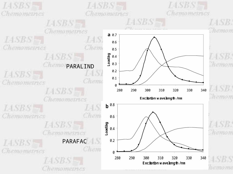
The results shown for three components indicate that similar results are obtained for PARAFAC and PARALIND with respect to predictions.

In order to test a four-component model, a single experiment

was modeled with both PARAFAC and PARALIND. In each

case, the model was refitted leaving out one sample at a time in

order to monitor how stable the model would be towards

changes in the data.

400 450 500 5500

0.02

0.04

0.06

0.08

0.1

0.12

Analyte loading

PARAFAC

400 450 500 5500

0.02

0.04

0.06

0.08

0.1

0.12

0.14

0.16

Additional loadings

400 450 500 5500

0.02

0.04

0.06

0.08

0.1

Analyte loading

PARALIND

400 450 500 5500

0.02

0.04

0.06

0.08

0.1

0.12

0.14

0.16

Additional loadings

1 1.5 2 2.5 3 3.5 4 4.5 52

4

6

8

10

12

14

16

Sample Loading for PARALIND

1 1.5 2 2.5 3 3.5 4 4.5 50

500

1000

1500

2000

2500

3000

3500

4000

4500

5000

PARAFAC

1 1.5 2 2.5 3 3.5 4 4.5 50

500

1000

1500

2000

2500

3000

3500

4000

4500

5000

As shown in Fig., the PARALIND model is very stable and provides spectral estimates that are consistent across samples as well as consistent with the overall model.

Hence, PARAFAC is not able to predict the analyte concentration and this points to the main advantage of using PARALIND for second order standard addition. Even when possibly minor components are included, the model results remain stable.

PARAFAC on the other hand, fails completely to model the analyte spectrum because the analyte spectrum becomes mixed up with one of the interference spectra.

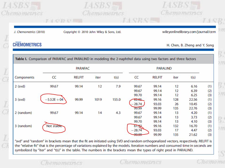
2)2) Comparison of PARAFAC and PARALIND in modeling three-way

fluorescence data array with special linear dependences in three modes: a

case study in 2-naphthol

2)2) Comparison of PARAFAC and PARALIND in modeling three-way

fluorescence data array with special linear dependences in three modes: a

case study in 2-naphthol

The EEMs of 2-naphthol with linear dependencies in three

modes are very different than any reported EEMs in the

literature.

J. Chemometrics (2010) Hao Chen, Binghui Zheng, Yonghui Song

It was concluded in this paper that whether a proper fit

would be obtained depends on how to properly put constraint

in the profile matrices (B and C) in PARALIND. When dealing

with complicated environmental samples without a priori

knowledge of the spectra characteristics of the underlying factors,

PARAFAC rather than PARALIND would be employed by the

investigators.

The presence of very overlapping spectra as well as fairly

good fit (e.g. small residuals) despite negative CC may function as

an ‘‘alarm’’ that linear dependences in some modes due to

complex physical/chemical processes are present, and great care

must be taken in interpreting the data.

However, the concentration profiles became

unique and chemically meaningful. Compared with

uninformed PARAFAC, PARALIND therefore improves the fit

on recovery of concentrations of collinear factors in this

example.

There has been increasing concern about linear

dependencies in three-mode data, for instance sample-pH-

absorbance data and sample-kinetic-spectra data .

PARALIND is a constrained form of PARAFACconstrained form of PARAFAC, and it can

be implemented by means of imposing proper constraints in

PARAFAC codes.

3 3

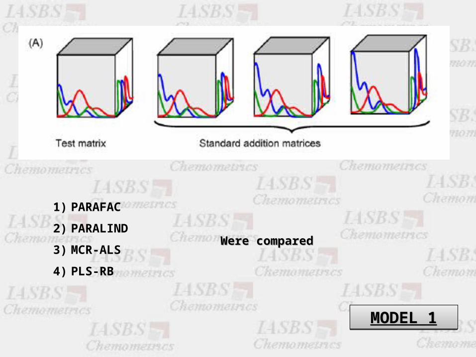
1) PARAFAC

2) PARALIND

3) MCR-ALS

4) PLS-RB

Were comparedWere compared

MODEL 1MODEL 1MODEL 1MODEL 1

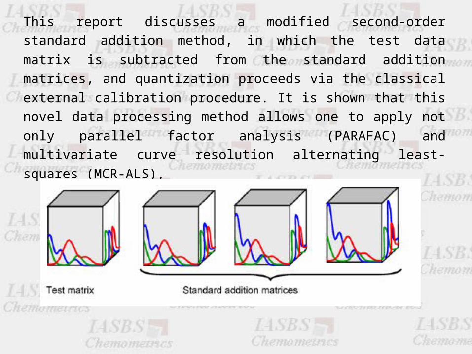
This report discusses a modified second-order standard addition

method, in which the test data matrix is subtracted from the standard

addition matrices, and quantization proceeds via the classical external

calibration procedure. It is shown that this novel data processing method

allows one to apply not only parallel factor analysis (PARAFAC) and

multivariate curve resolution alternating least-squares (MCR-ALS),

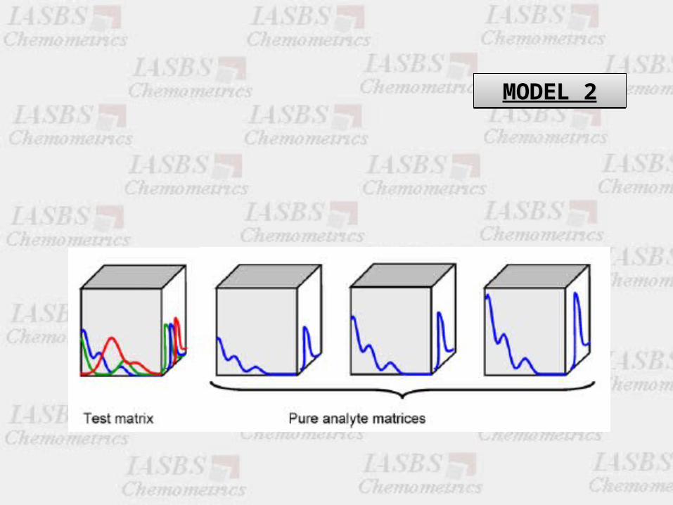
MODEL 2MODEL 2MODEL 2MODEL 2

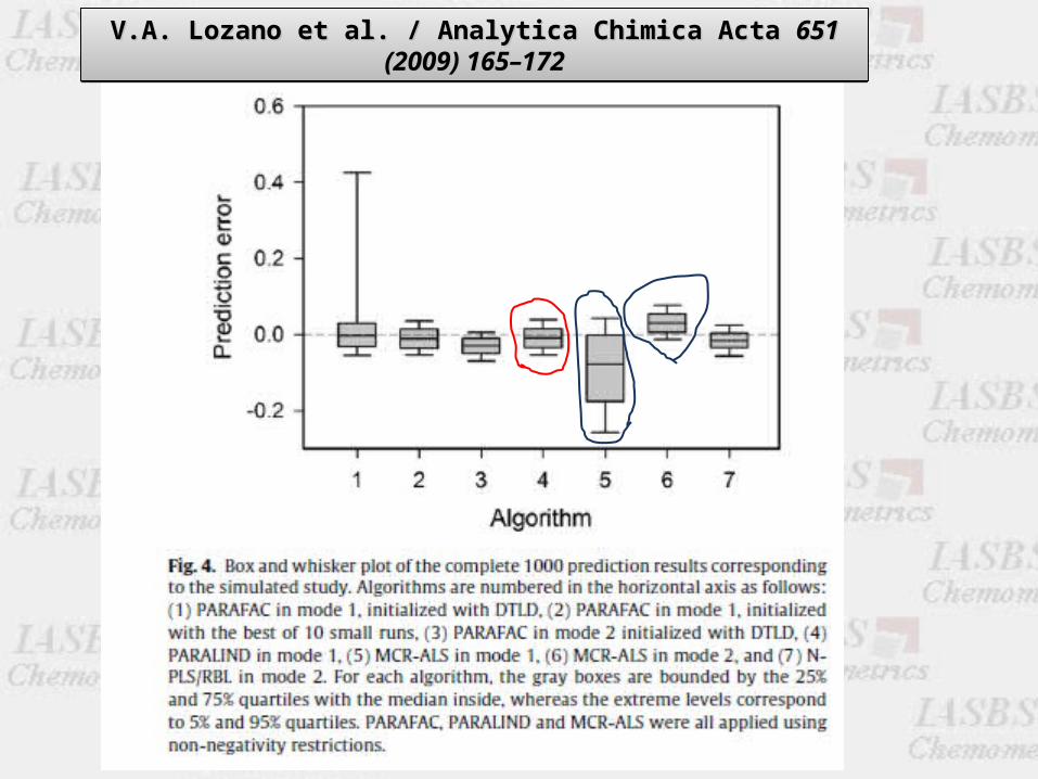
V.A. Lozano et al. / Analytica Chimica Acta V.A. Lozano et al. / Analytica Chimica Acta 651 (2009) 165–172651 (2009) 165–172V.A. Lozano et al. / Analytica Chimica Acta V.A. Lozano et al. / Analytica Chimica Acta 651 (2009) 165–172651 (2009) 165–172

For MCR-ALS results; inspection of this Fig.

reveals a bias in the complete results using model 1,

with a significant improvement on employment of

model 2 (in fact, the small remaining bias is

comparable to the uncertainty in nominal

concentrations, i.e., 0.01 units). The origin of the bias

in the former case is unclear, but may be related to

the strong correlations when mode 1 is used.

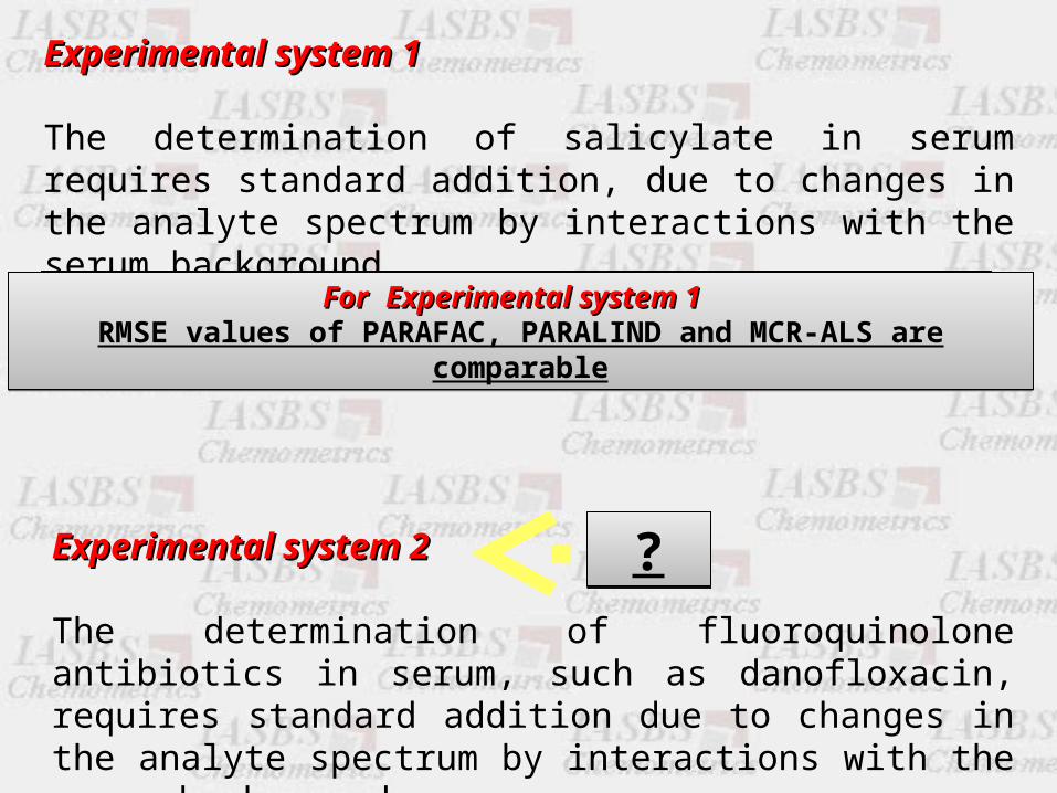
Experimental system 1Experimental system 1

The determination of salicylate in serum requires standard addition, due to changes in the analyte spectrum by interactions with the serum background.

Experimental system 2Experimental system 2

The determination of fluoroquinolone antibiotics in serum, such as danofloxacin, requires standard addition due to changes in the analyte spectrum by interactions with the serum background

Both experimental data were estimated to have 3 componentsBoth experimental data were estimated to have 3 componentsForFor Experimental system 1Experimental system 1 RMSE values of PARAFAC, PARALIND and MCR-ALS are comparable

ForFor Experimental system 1Experimental system 1 RMSE values of PARAFAC, PARALIND and MCR-ALS are comparable

??

AlgorithmPARAFACModel 2

PARALINDMCR-ALSModel2

RMSE101030

For Experimental system 2For Experimental system 2Specific prediction results for the set of spiked test samples

In this case, where lower sensitivity towards the analyte is attained, and

heavy spectral overlapping occurs in both data dimensions, the RMSE is

rather high in comparison with the mean analyte concentration across the

set of samples. As with the previous experimental system, the prediction

results obtained from PARALIND were identical to those corresponding to

PARAFAC model 2.

When applying MCR-ALS, the predictions were clearly worse,

indicating that the combination of low analyte signal and spectral

overlapping have a stronger effect on this algorithm than on PARAFAC

decomposition.

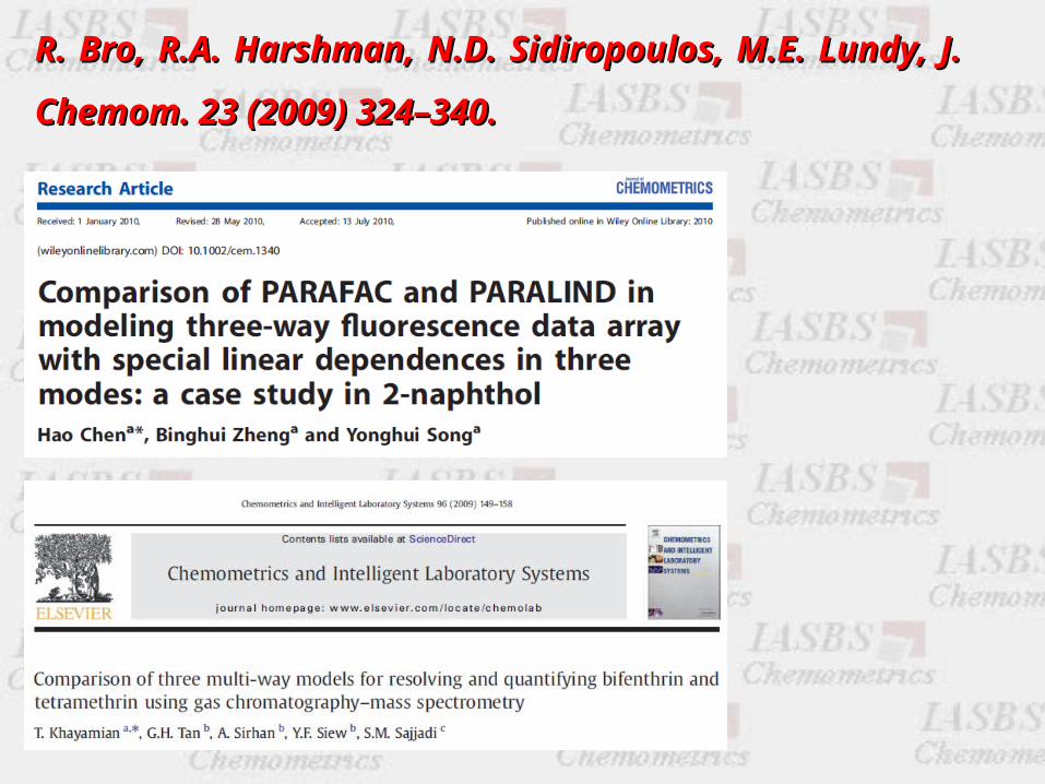
R. Bro, R.A. Harshman, N.D. Sidiropoulos, M.E. Lundy, R. Bro, R.A. Harshman, N.D. Sidiropoulos, M.E. Lundy,

J. Chemom. 23 (2009) 324–340.J. Chemom. 23 (2009) 324–340.

Want to know more and downlod some mfiles Look at Rasmus Bro’s website

Thanks for your attentions

Any question