Impact of Doppler Lidar radial wind data

assimilation to a localized heavy rainfall event

Takuya Kawabata1, Hironori Iwai2, Hiromu Seko1, Yoshinori Shoji1, Kazuo Saito1

1Meteorological Research Institute / Japan Meteorological Agency 2National Institute of Information and Communications Technology (NICT)

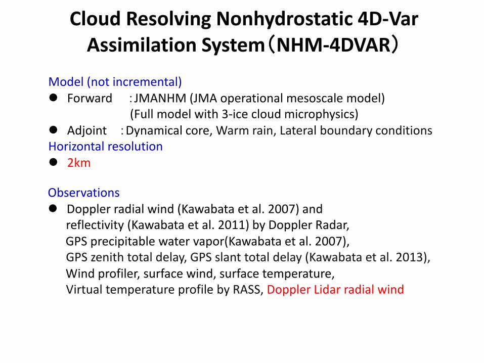
Cloud Resolving Nonhydrostatic 4D-Var Assimilation System（NHM-4DVAR）

Model (not incremental) Forward ：JMANHM (JMA operational mesoscale model) (Full model with 3-ice cloud microphysics) Adjoint ：Dynamical core, Warm rain, Lateral boundary conditions Horizontal resolution 2km

Observations Doppler radial wind (Kawabata et al. 2007) and reflectivity (Kawabata et al. 2011) by Doppler Radar, GPS precipitable water vapor(Kawabata et al. 2007), GPS zenith total delay, GPS slant total delay (Kawabata et al. 2013), Wind profiler, surface wind, surface temperature, Virtual temperature profile by RASS, Doppler Lidar radial wind

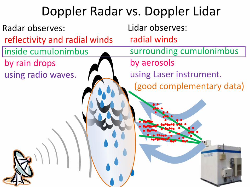
Doppler Radar vs. Doppler Lidar Radar observes: reflectivity and radial winds inside cumulonimbus by rain drops using radio waves.

Lidar observes: radial winds surrounding cumulonimbus by aerosols using Laser instrument. (good complementary data)

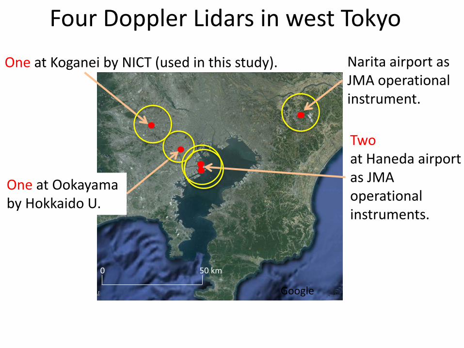
Four Doppler Lidars in west Tokyo

Google

0 50 km

Two at Haneda airport as JMA operational instruments.

One at Koganei by NICT (used in this study).

One at Ookayama by Hokkaido U.

Narita airport as JMA operational instrument.

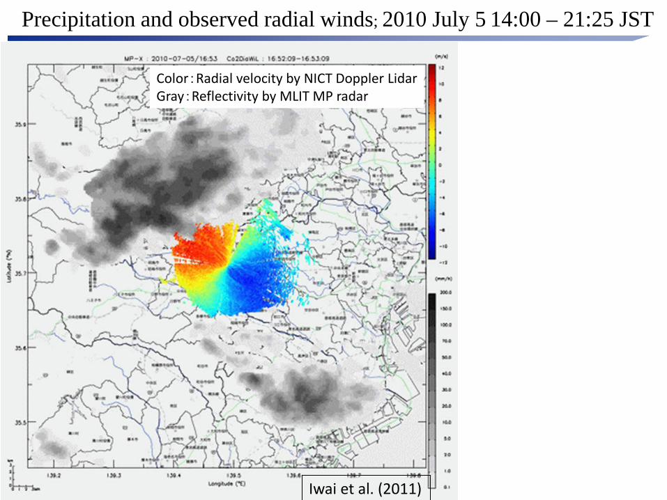
Color：Radial velocity by NICT Doppler Lidar Gray：Reflectivity by MLIT MP radar

Precipitation and observed radial winds; 2010 July 5 14:00 – 21:25 JST

Iwai et al. (2011)

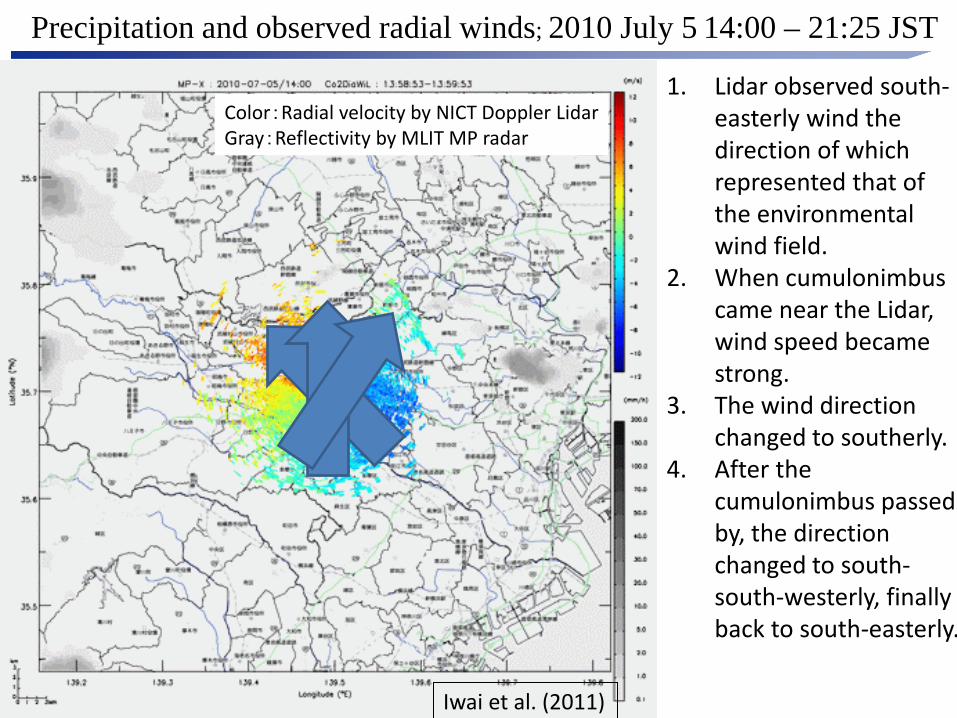
Color：Radial velocity by NICT Doppler Lidar Gray：Reflectivity by MLIT MP radar

Precipitation and observed radial winds; 2010 July 5 14:00 – 21:25 JST

Iwai et al. (2011)

1. Lidar observed south-easterly wind the direction of which represented that of the environmental wind field.

2. When cumulonimbus came near the Lidar, wind speed became strong.

3. The wind direction changed to southerly.

4. After the cumulonimbus passed by, the direction changed to south-south-westerly, finally back to south-easterly.

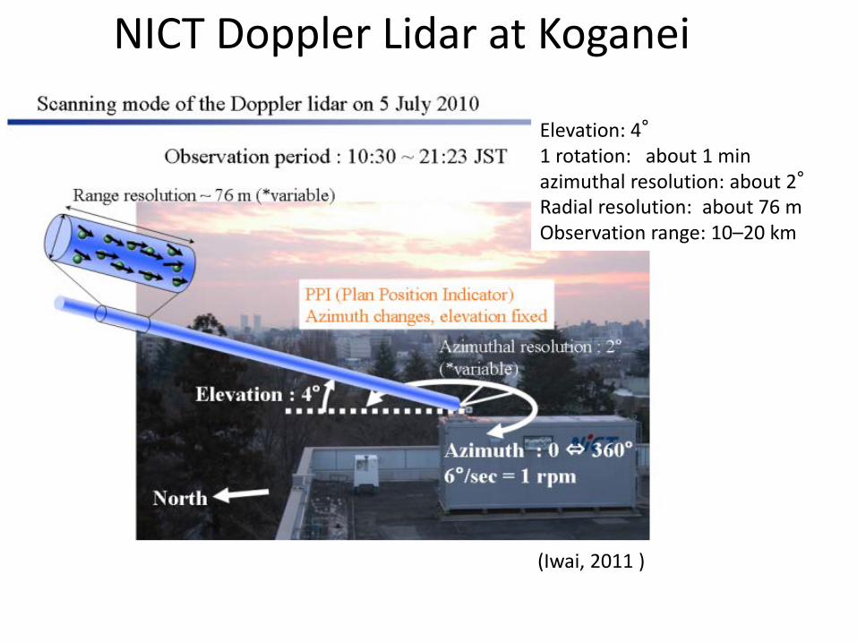
Elevation: 4° 1 rotation: about 1 min azimuthal resolution: about 2° Radial resolution: about 76 m Observation range: 10–20 km

NICT Doppler Lidar at Koganei

(Iwai, 2011 )

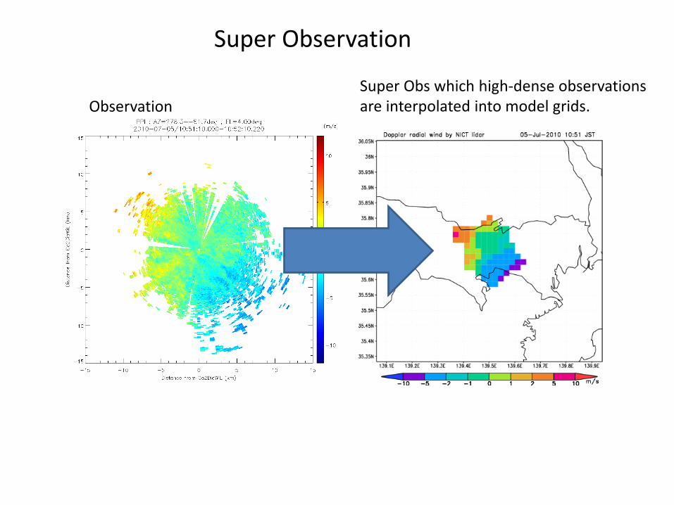
Super Observation

Observation Super Obs which high-dense observations are interpolated into model grids.

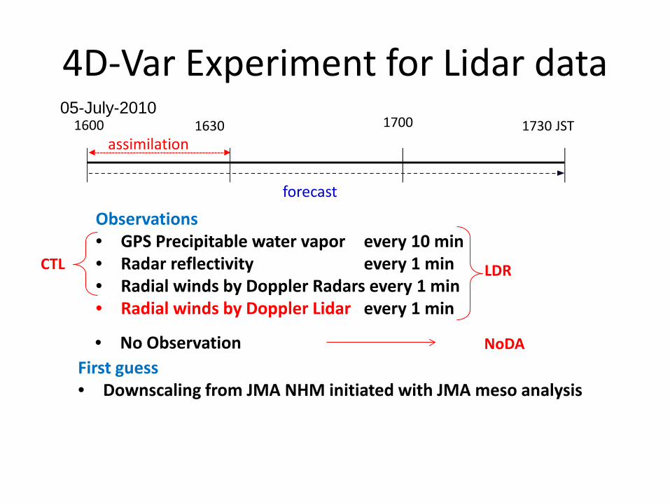
4D-Var Experiment for Lidar data 05-July-2010

1600 1630 1700 1730 JST assimilation

forecast Observations • GPS Precipitable water vapor every 10 min • Radar reflectivity every 1 min • Radial winds by Doppler Radars every 1 min • Radial winds by Doppler Lidar every 1 min

First guess • Downscaling from JMA NHM initiated with JMA meso analysis

CTL LDR

NoDA • No Observation

A

B

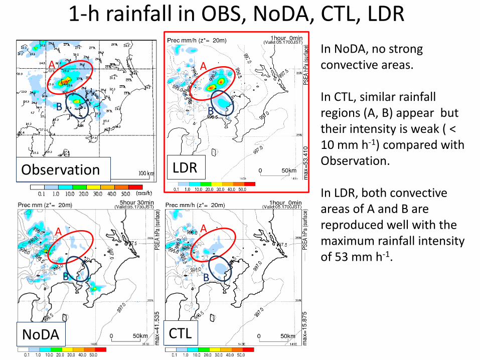
1-h rainfall in OBS, NoDA, CTL, LDR

A

B B

A

B

A

NoDA

Observation

CTL

LDR

In NoDA, no strong convective areas. In CTL, similar rainfall regions (A, B) appear but their intensity is weak ( < 10 mm h-1) compared with Observation. In LDR, both convective areas of A and B are reproduced well with the maximum rainfall intensity of 53 mm h-1.

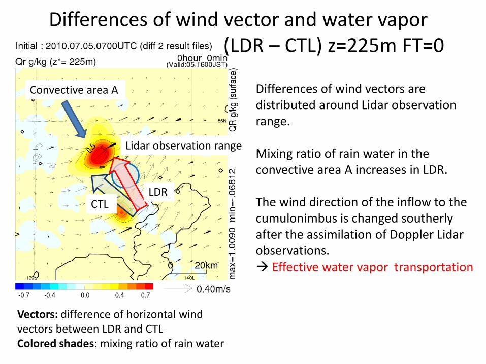
Differences of wind vector and water vapor (LDR – CTL) z=225m FT=0

Lidar observation range

Differences of wind vectors are distributed around Lidar observation range. Mixing ratio of rain water in the convective area A increases in LDR. The wind direction of the inflow to the cumulonimbus is changed southerly after the assimilation of Doppler Lidar observations. Effective water vapor transportation

CTL

Convective area A

LDR

Vectors: difference of horizontal wind vectors between LDR and CTL Colored shades: mixing ratio of rain water

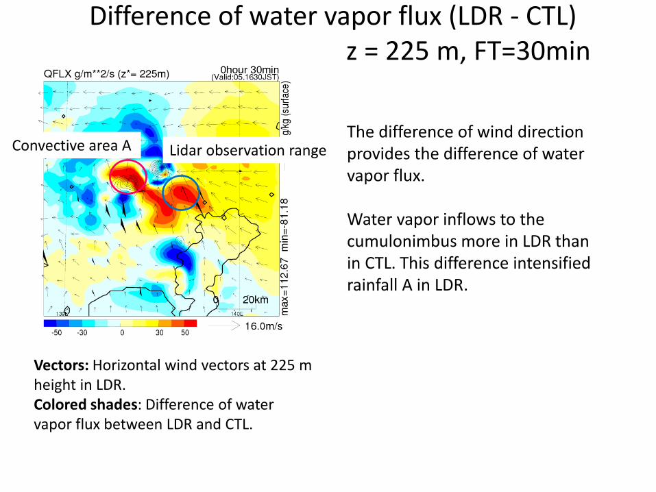
Difference of water vapor flux (LDR - CTL) z = 225 m, FT=30min

Lidar observation range Convective area A The difference of wind direction provides the difference of water vapor flux. Water vapor inflows to the cumulonimbus more in LDR than in CTL. This difference intensified rainfall A in LDR.

Vectors: Horizontal wind vectors at 225 m height in LDR. Colored shades: Difference of water vapor flux between LDR and CTL.

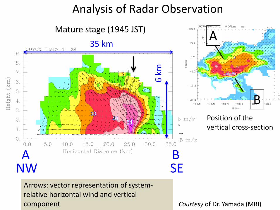
Mature stage (1945 JST)

A B NW SE

35 km

6 km

A

B Position of the vertical cross-section

Arrows: vector representation of system-relative horizontal wind and vertical component Courtesy of Dr. Yamada (MRI)

Analysis of Radar Observation

A B

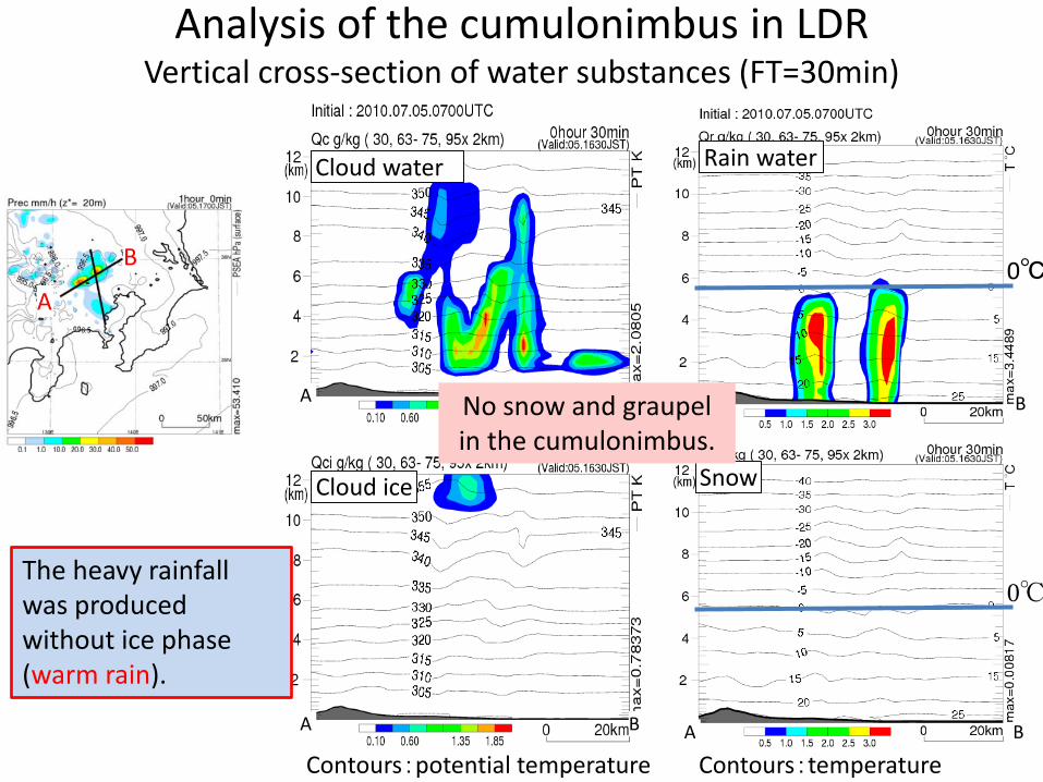
Cloud water

Analysis of the cumulonimbus in LDR Vertical cross-section of water substances (FT=30min)

Contours：temperature

0℃ A

B

Contours：potential temperature

Rain water

Cloud ice Snow

A B A B

A B

No snow and graupel in the cumulonimbus.

0℃ The heavy rainfall was produced without ice phase (warm rain).

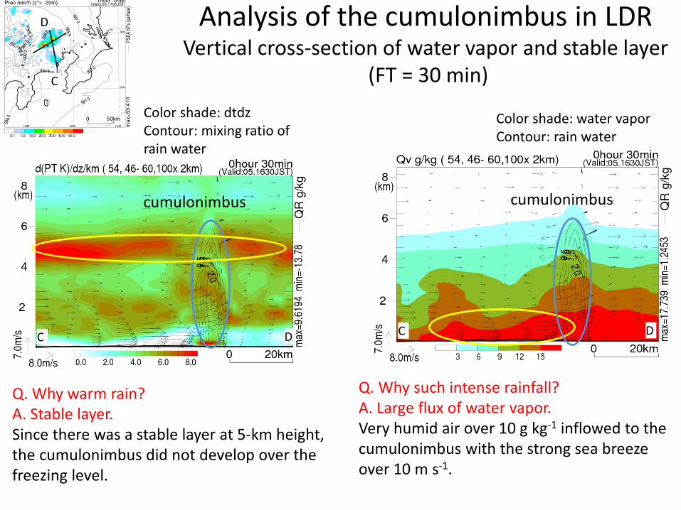
Analysis of the cumulonimbus in LDR Vertical cross-section of water vapor and stable layer

(FT = 30 min)

C D C D

Color shade: water vapor Contour: rain water

Q. Why such intense rainfall? A. Large flux of water vapor. Very humid air over 10 g kg-1 inflowed to the cumulonimbus with the strong sea breeze over 10 m s-1.

Q. Why warm rain? A. Stable layer. Since there was a stable layer at 5-km height, the cumulonimbus did not develop over the freezing level.

C

D

cumulonimbus cumulonimbus

Color shade: dtdz Contour: mixing ratio of rain water

Summary • Data assimilation experiment was conducted on the Itabashi

heavy rainfall event using NHM-4DVAR. • Assimilated observations are radial wind by Doppler Lidar,

radial wind by Doppler Radar, radar reflectivity, and GPS precipitable water vapor.

• By assimilating Doppler Lidar data, the intense rainfall region was forecasted similar to the observation.

• Because of the stable layer, the cumulonimbus did not developed over the freezing level.

• Large water vapor flux induced the heavy rainfall.