Hybrid cell-centred/vertex model for multicellular systems
126
Hybrid cell-centred/vertex model for multicellular systems Payman Mosaffa ADVERTIMENT La consulta d’aquesta tesi queda condicionada a l’acceptació de les següents condicions d'ús: La difusió d’aquesta tesi per mitjà del repositori institucional UPCommons (http://upcommons.upc.edu/tesis) i el repositori cooperatiu TDX ( http://www.tdx.cat/ ) ha estat autoritzada pels titulars dels drets de propietat intel·lectual únicament per a usos privats emmarcats en activitats d’investigació i docència. No s’autoritza la seva reproducció amb finalitats de lucre ni la seva difusió i posada a disposició des d’un lloc aliè al servei UPCommons o TDX. No s’autoritza la presentació del seu contingut en una finestra o marc aliè a UPCommons (framing). Aquesta reserva de drets afecta tant al resum de presentació de la tesi com als seus continguts. En la utilització o cita de parts de la tesi és obligat indicar el nom de la persona autora. ADVERTENCIA La consulta de esta tesis queda condicionada a la aceptación de las siguientes condiciones de uso: La difusión de esta tesis por medio del repositorio institucional UPCommons (http://upcommons.upc.edu/tesis) y el repositorio cooperativo TDR (http://www.tdx.cat/?locale- attribute=es) ha sido autorizada por los titulares de los derechos de propiedad intelectual únicamente para usos privados enmarcados en actividades de investigación y docencia. No se autoriza su reproducción con finalidades de lucro ni su difusión y puesta a disposición desde un sitio ajeno al servicio UPCommons No se autoriza la presentación de su contenido en una ventana o marco ajeno a UPCommons (framing). Esta reserva de derechos afecta tanto al resumen de presentación de la tesis como a sus contenidos. En la utilización o cita de partes de la tesis es obligado indicar el nombre de la persona autora. WARNING On having consulted this thesis you’re accepting the following use conditions: Spreading this thesis by the institutional repository UPCommons (http://upcommons.upc.edu/tesis) and the cooperative repository TDX (http://www.tdx.cat/?locale- attribute=en) has been authorized by the titular of the intellectual property rights only for private uses placed in investigation and teaching activities. Reproduction with lucrative aims is not authorized neither its spreading nor availability from a site foreign to the UPCommons service. Introducing its content in a window or frame foreign to the UPCommons service is not authorized (framing). These rights affect to the presentation summary of the thesis as well as to its contents. In the using or citation of parts of the thesis it’s obliged to indicate the name of the author.
Transcript of Hybrid cell-centred/vertex model for multicellular systems

Hybrid cell-centred/vertex model for multicellular systems
Payman Mosaffa
ADVERTIMENT La consulta d’aquesta tesi queda condicionada a l’acceptació de les següents condicions d'ús: La difusió d’aquesta tesi per mitjà del r e p o s i t o r i i n s t i t u c i o n a l UPCommons (http://upcommons.upc.edu/tesis) i el repositori cooperatiu TDX ( h t t p : / / w w w . t d x . c a t / ) ha estat autoritzada pels titulars dels drets de propietat intel·lectual únicament per a usos privats emmarcats en activitats d’investigació i docència. No s’autoritza la seva reproducció amb finalitats de lucre ni la seva difusió i posada a disposició des d’un lloc aliè al servei UPCommons o TDX. No s’autoritza la presentació del seu contingut en una finestra o marc aliè a UPCommons (framing). Aquesta reserva de drets afecta tant al resum de presentació de la tesi com als seus continguts. En la utilització o cita de parts de la tesi és obligat indicar el nom de la persona autora.
ADVERTENCIA La consulta de esta tesis queda condicionada a la aceptación de las siguientes condiciones de uso: La difusión de esta tesis por medio del repositorio institucional UPCommons (http://upcommons.upc.edu/tesis) y el repositorio cooperativo TDR (http://www.tdx.cat/?locale-attribute=es) ha sido autorizada por los titulares de los derechos de propiedad intelectual únicamente para usos privados enmarcados en actividades de investigación y docencia. No se autoriza su reproducción con finalidades de lucro ni su difusión y puesta a disposición desde un sitio ajeno al servicio UPCommons No se autoriza la presentación de su contenido en una ventana o marco ajeno a UPCommons (framing). Esta reserva de derechos afecta tanto al resumen de presentación de la tesis como a sus contenidos. En la utilización o cita de partes de la tesis es obligado indicar el nombre de la persona autora.
WARNING On having consulted this thesis you’re accepting the following use conditions: Spreading this thesis by the i n s t i t u t i o n a l r e p o s i t o r y UPCommons (http://upcommons.upc.edu/tesis) and the cooperative repository TDX (http://www.tdx.cat/?locale-attribute=en) has been authorized by the titular of the intellectual property rights only for private uses placed in investigation and teaching activities. Reproduction with lucrative aims is not authorized neither its spreading nor availability from a site foreign to the UPCommons service. Introducing its content in a window or frame foreign to the UPCommons service is not authorized (framing). These rights affect to the presentation summary of the thesis as well as to its contents. In the using or citation of parts of the thesis it’s obliged to indicate the name of the author.

Universitat Politecnica de Catalunya
Laboratori de Calcul Numeric
Doctor of Philosophy in Applied Mathematics
Hybrid Cell-centred/Vertex Model for
Multicellular Systems
Author
Payman Mosaffa
Supervisor
Jose Javier Munoz Romero
Barcelona, September 2017
( )
La
Cà
N·


Abstract
This thesis presents a hybrid vertex/cell-centred approach to mechanically sim-ulate planar cellular monolayers undergoing cell reorganisation. Cell centres arerepresented by a triangular nodal network, while the cell boundaries are formed byan associated vertex network. The two networks are coupled through a kinematicconstraint which we allow to relax progressively. Cell-cell connectivity changes dueto cell reorganisation or remodelling events, are accentuated. These situations arehandled by using a variable resting length and applying an Equilibrium-PreservingMapping (EPM) on the new connectivity, which computes a new set of restinglengths that preserve nodal and vertex equilibrium. As a by-product, the proposedtechnique enables to recover fully vertex or fully cell-centred models in a seamlessmanner by modifying a numerical parameter of the model. The properties of themodel are illustrated by simulating monolayers subjected to imposed extension andduring a wound healing process. The evolution of forces and the EPM are analysedduring the remodelling events.
v

Resumen
Esta tesis presenta un modelo hıbrido para la simulacion mecanica de monocapascelulares. Este modelo combina metodos de vertices y centrados en la celula, yesta orientado al analisis de deformaciones con reorganizacion celular. Los nucleosvienen representados por nodos que forman una malla triangular, mientras que lascontornos (membranas y cortex) forman una malla poligonal de vertices. Las dosmallas se acoplan a traves de una restriccion cinematica que puede ser relajada deforma controlada. El estudio hace especial hincapie en los cambios de conectividad,tanto debidos a la reorganizacion celular como el remodelado del citoesqueleto. Estassituaciones se abordan a traves de una longitud de referencia variable y aplicando unMapeo con Conservacion de Equilibrio (EPM) que minimiza el error en el equilibrionodal y en los vertices. La tecnica resultante puede ser adaptada progresivamente atraves de un parametro, dando lugar a un modelo exclusivamente de vertices o a unode centros. Sus propiedades se ilustran en simulaciones de monocapas sujetas a unaextension impuesta y durante el proceso de cicatrizado de heridas. La evolucionde las fuerzas y los efectos del EPM durante el remodelado se analizan en estosejemplos.
vii

Acknowledgements
First and foremost, I would like to express my sincere gratitude to my advi-sor Prof. Jose Javier Munoz for the continuous support of my Ph.D study andrelated research, for his patience, motivation, immense knowledge, and wonderfulmentorship.
I also appreciate Prof. Yanlan Mao and Prof. Antonio Rodrıguez-Ferran fortheir fruitful advices and great guidance. Besides, I would like to thank Dr. DanielMillan and Dr. Rob Tetly for their collaboration and helpful comments.
I would like to express my thanks to all my colleagues at LaCaN, UPC, whom Iam sincerely feel grateful to, especially Dr. Nina Asadipour.
During my two two-month visits at Laboratory for Molecular Cell Biology (LMCB)at University College London, I had the chance to collaborate and discuss relatedtopics with wonderful people. Among them I feel especially fortunate to know Dr.Melda Tozluoglu and Dr. Nargess Khalilgharibi.
I acknowledge the partial financial support of the Spanish Ministry of Econ-omy, Science and Competitiveness (MINECO) under grants DPI2013-32727-R andDPI2016-74929-R, Generalitat de Catalunya under grant 2014-SGR-1471, EuropeanMolecular Biology Organisation (EMBO) under grant ASTF 351-2016, and founda-tion Ferran Sunyer i Balaguer under grant FSB 2015.
Last but not the least, I would like to thank my family. Words cannot expresshow grateful I am to my parents for all of the sacrifices that you have made on mybehalf.
ix


Contents
Abstract v
Resumen vii
Acknowledgements ix
1 State of the art 11.1 Biological background . . . . . . . . . . . . . . . . . . . . . . . . . . 11.2 Modelling in tissue biology . . . . . . . . . . . . . . . . . . . . . . . 3
1.2.1 Modelling scale and predictability . . . . . . . . . . . . . . . 31.2.2 Major modelling approaches . . . . . . . . . . . . . . . . . . . 3
1.3 Objectives and proposed model . . . . . . . . . . . . . . . . . . . . . 61.4 Outline . . . . . . . . . . . . . . . . . . . . . . . . . . . . . . . . . . 8
2 Tissue discretisation 112.1 Cell-centred model . . . . . . . . . . . . . . . . . . . . . . . . . . . . 11
2.1.1 Cell-centred mechanical equilibrium . . . . . . . . . . . . . . 122.1.2 Cell-cell connectivity: modified Delaunay triangulation . . . . 142.1.3 Remodelling of cell-centred model: L-tensor method . . . . . 172.1.4 Cell-centred model for curved monolayers . . . . . . . . . . . 182.1.5 Cells boundary . . . . . . . . . . . . . . . . . . . . . . . . . . 22
2.2 Hybrid model . . . . . . . . . . . . . . . . . . . . . . . . . . . . . . . 252.2.1 Vertex geometry and barycentric tessellation . . . . . . . . . 262.2.2 Vertex mechanical equilibrium . . . . . . . . . . . . . . . . . 272.2.3 Area constraint . . . . . . . . . . . . . . . . . . . . . . . . . . 302.2.4 ξ-Relaxation . . . . . . . . . . . . . . . . . . . . . . . . . . . 322.2.5 Remodelling: Equilibrium Preserving Mapping . . . . . . . . 34
3 Rheological model 393.1 Elastic model . . . . . . . . . . . . . . . . . . . . . . . . . . . . . . . 393.2 Kelvin-Voigt and Maxwell models . . . . . . . . . . . . . . . . . . . . 40
3.2.1 Implementation of Kelvin-Voigt model . . . . . . . . . . . . . 413.2.2 Implementation of Maxwell model . . . . . . . . . . . . . . . 41
xi

xii CONTENTS
3.3 Active model . . . . . . . . . . . . . . . . . . . . . . . . . . . . . . . 41
3.3.1 Linear active model . . . . . . . . . . . . . . . . . . . . . . . 42
3.3.2 Non-linear active model (power law) . . . . . . . . . . . . . . 44
4 Numerical Results 47
4.1 Extension of cell-centred networks . . . . . . . . . . . . . . . . . . . 47
4.2 Active rheology in flat monolayers . . . . . . . . . . . . . . . . . . . 50
4.3 Active rheology in curved monolayers . . . . . . . . . . . . . . . . . 53
4.4 Extension of square tissue employing hybrid model . . . . . . . . . . 55
4.4.1 Verification of EPM: fixed topology . . . . . . . . . . . . . . 56
4.4.2 Verification of EPM: variable topology . . . . . . . . . . . . . 57
4.4.3 Analysis of ξ-relaxation . . . . . . . . . . . . . . . . . . . . . 59
4.5 Wound healing . . . . . . . . . . . . . . . . . . . . . . . . . . . . . . 61
4.6 Short timescale stress relaxation in monolayers . . . . . . . . . . . . 65
5 Conclusions 69
6 Future work 73
6.1 Mapping of new vertices . . . . . . . . . . . . . . . . . . . . . . . . . 73
6.2 Three-dimensional extension of cellular monolayers and aggregates . 73
6.3 Calibration of parameters . . . . . . . . . . . . . . . . . . . . . . . . 74
6.4 Strain dependent contractility . . . . . . . . . . . . . . . . . . . . . . 75
6.5 Definition of stress and transport in Delaunay . . . . . . . . . . . . . 75
6.6 Oscillations . . . . . . . . . . . . . . . . . . . . . . . . . . . . . . . . 75
A Notation 77
B Inradius and circumradius 81
B.1 Inradius . . . . . . . . . . . . . . . . . . . . . . . . . . . . . . . . . . 81
B.2 Circumradius . . . . . . . . . . . . . . . . . . . . . . . . . . . . . . . 82
B.3 Aspect ratio of triangles . . . . . . . . . . . . . . . . . . . . . . . . . 83
B.4 Aspect ratio of tetrahedrons . . . . . . . . . . . . . . . . . . . . . . . 84
C Proof of uniqueness of active length tensor Li 87
D Voronoi diagram 89
E Linearisation 91
E.1 General linearisation steps with ξ-relaxation . . . . . . . . . . . . . . 91
E.2 Linearisation of nodal and vertex tractions tijD and tIJV . . . . . . . . 92
E.3 Linearisation terms in Kijxx . . . . . . . . . . . . . . . . . . . . . . . 93
E.4 Linearisation terms in KiJxy . . . . . . . . . . . . . . . . . . . . . . . 94
E.5 Linearisation terms in KIJyy . . . . . . . . . . . . . . . . . . . . . . . 94

CONTENTS xiii
Bibliography 95


List of Figures
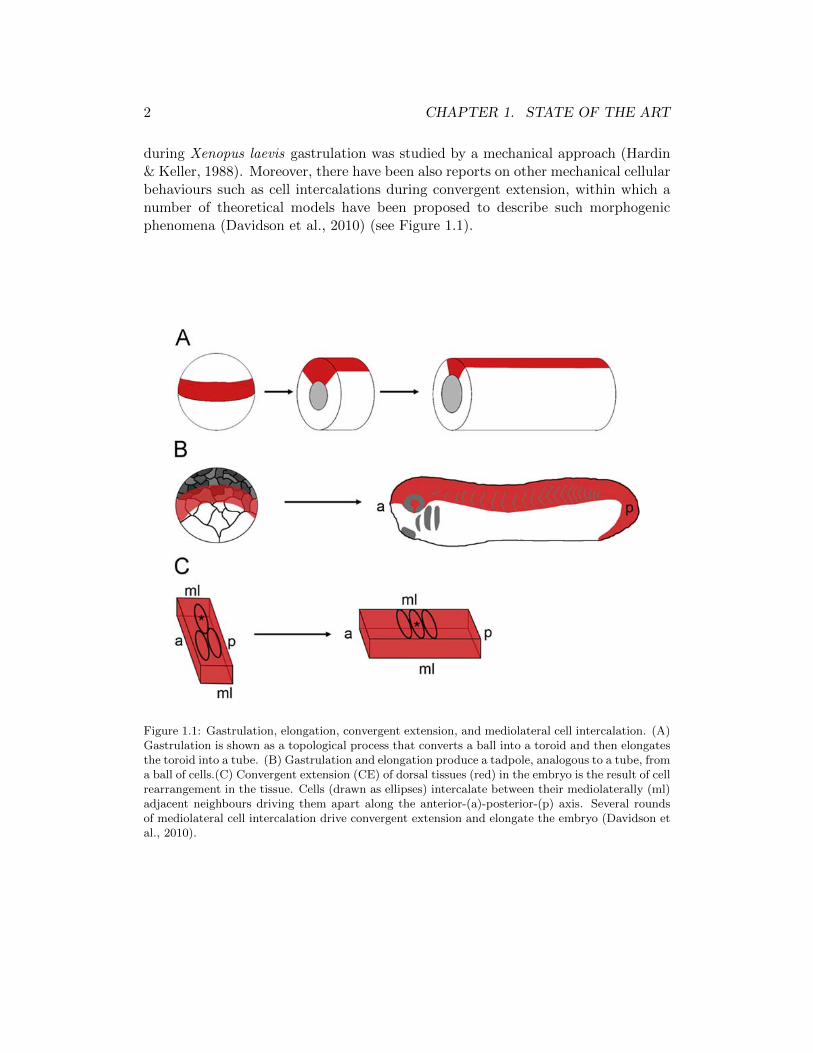
1.1 Gastrulation, elongation, convergent extension, and mediolateral cellintercalation. (A) Gastrulation is shown as a topological process thatconverts a ball into a toroid and then elongates the toroid into a tube.(B) Gastrulation and elongation produce a tadpole, analogous to atube, from a ball of cells.(C) Convergent extension (CE) of dorsal tis-sues (red) in the embryo is the result of cell rearrangement in the tis-sue. Cells (drawn as ellipses) intercalate between their mediolaterally(ml) adjacent neighbours driving them apart along the anterior-(a)-posterior-(p) axis. Several rounds of mediolateral cell intercalationdrive convergent extension and elongate the embryo (Davidson et al.,2010). . . . . . . . . . . . . . . . . . . . . . . . . . . . . . . . . . . . 2
2.1 Two-step update process of nodal configuration. (a) ConfigurationCn = Xn,T n at time tn, (b) Nodal configurationC∗n+1 = Xn+1,T nafter obtaining mechanical equilibrium, and (c) configuration Cn+1 =Xn+1,T n+1 at time tn+1. . . . . . . . . . . . . . . . . . . . . . . . 12
2.2 Schematic view of node i connectivity (continuous lines), within therest of the network (dashed lines) and traction vector tijD. . . . . . . 14
2.3 Triangulation of set of points P = A,B,C,D,E. (a) non-Delaunaytriangulation as points B and C are inside the circumcircle of4ADE.(b) non-Delaunay triangulation as point C is inside the circumcircleof 4ABE. (c) Delaunay triangulation as there is no point inside thecircumcircle of either of triangles. . . . . . . . . . . . . . . . . . . . . 15
2.4 Modified Delaunay triangulation of set of points P . (a) Distributionof set of points P in the plane. (b) Standard Delaunay triangulationof set of points P ; skinny triangles covering the concave edge of thenetwork are marked in green. (c) Modified Delaunay triangulation ofset of points P by the application of the filtering process on DT (P ). 15
2.5 Incircle I and circumcircle O of 4ABC. r and R are inradius andcircumradius of 4ABC respectively. . . . . . . . . . . . . . . . . . . 16
xv
xvi LIST OF FIGURES
2.6 Schematic of computational process for retrieving nodal positionsan connectivity Xn+1,T n+1 from the same quantities at time tn.(a)→(b): computation of new positions Xn+1 from mechanical equi-librium. (b)→(c): computation of new connectivity T n+1 from De-launay triangulation. (c)→(d): trimming of Delaunay connectivityT n+1, resulting in a not necessarily convex boundary of the cell-centred network T n+1. . . . . . . . . . . . . . . . . . . . . . . . . . . 17
2.7 (a) Arbitrary point set configuration from a proof of concept exam-ple in 3-D. (b) Two-dimensional embedding obtained by using MLLE(Zhang & Wang, 2007)(k-nn=8). The lack of metric related to theinput data, that is, different distances between points in the realand mapped domain, and its unit covariance (mapped points are dis-tributed on a squared region) are apparent from the picture. (c)Two-dimensional embedding nodes and connectivity after applyingthe filtering described in Section 2.1.2. (d) Three-dimensional initialpoint set configuration with resulting connectivity. The colour-map,which indicates the identifier of each sample of the point set, is pro-vided for visual inspection. . . . . . . . . . . . . . . . . . . . . . . . 20
2.8 Top: monolayer with half-cylinder geometry. The nodes at the planez = 0 are constrained to remain in the plane, while the nodes atthe other base of the half-cylinder are constrained to remain in planez = 5. Bottom: multiple rigid modes of the monolayer with half-cylinder geometry. . . . . . . . . . . . . . . . . . . . . . . . . . . . . 21
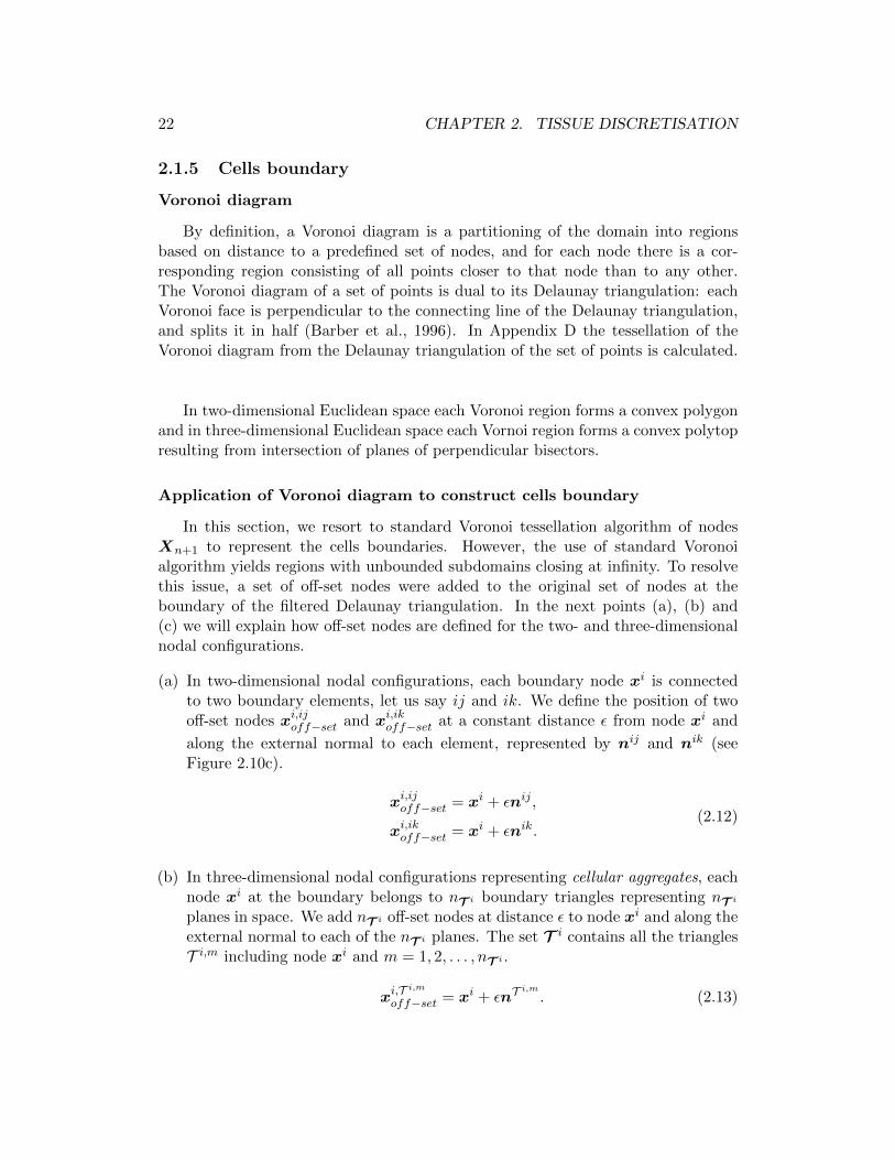
2.9 Schematic view of a monolayer in 3-D and construction of off-setnodes for the nodes on the middle and the edge of the monolayer. nand −n represent upward and downward normals to the surface ofeach triangle, following the same colour as the corresponding triangle.nij and nik are the normals to the edge elements ij and ik, and in theplane of triangles T i,p and T i,q, respectively. ε represents the distancebetween each off-set node with its corresponding original node. . . . 24
2.10 Voronoi tessellation. (a) Delaunay triangulation of original set ofnodes (T n+1 = DT (Xn+1)). (b) Voronoi tessellation of originalset of nodes resulting in open regions for the nodes the boundary(V n+1 = V or(Xn+1)). (c) construct off-set nodes at the boundary ofthe domain (Xn+1 = Xn+1,Xoff−set,n+1). (d) Delaunay triangu-lation of total nodal configuration (T n+1 = DT (Xn+1)), and obtaintotal Voronoi tessellation (V n+1 = V or(Xn+1)). (e) Remove off-setnodes and elements and obtain close regions for all original nodes. . 25
2.11 Discretisation of tissue into cell centres (nodes, xi) and cells bound-aries (vertices, yi). Nodal network and vertex network are outlinedwith continuous and dashed lines, respectively. . . . . . . . . . . . . 26

LIST OF FIGURES xvii
2.12 Differences between Voronoi (top) and barycentric vertex positions(bottom) for undeformed (left) and deformed networks (right).(a)Nodal network (in black) with Delaunay triangulation and vertexnetwork (in red) with Voronoi tessellation. (b) Deformed nodal net-work: non-Delaunay triangulation; vertices defined by interpolationof nodes in each triangle, located at the intersection of perpendicularbisectors of each triangle, forming a non-Voronoi vertex network. (c)Nodal network with Delaunay triangulation and vertex network withBarycentric tessellation. (d) Deformed nodal network: non-Delaunaytriangulation; vertices defined by interpolation of nodes in each trian-gle, located at the Barycentres of each triangle, forming a barycentricvertex network. . . . . . . . . . . . . . . . . . . . . . . . . . . . . . . 28
2.13 Cell boundary (highlighted polygon) corresponding to node i. Barycen-tric tessellation of 4ijk results to triple-junction yI . Vector tIJV rep-resents the traction between vertices yI and yJ along the sharedboundary of cells xi and xk. . . . . . . . . . . . . . . . . . . . . . . . 29
2.14 Deformation and remodelling process, including the computation ofthe resting lengths L∗n+1 through the Equilibrium-Preserving Map,which maintains the network connectivity and nodal and vertex po-sitions. . . . . . . . . . . . . . . . . . . . . . . . . . . . . . . . . . . . 35
3.1 Representation of (a) Kelvin-Voigt model and (b) Maxwell model. . 40
3.2 Generalised Maxwell model . . . . . . . . . . . . . . . . . . . . . . . 41
3.3 Left: Schematic of network of actin filaments connected by flexiblecross-links. Right: Schematic of strain induced changes in the restinglength L of a reduced system with two filaments and a cross-link(white circle), (a) initial configuration with resting length equal toL0, (b) configuration under an applied load, and (c) new unstrainedconfiguration with modified resting length L > L0. . . . . . . . . . . 43
4.1 Graphical representation of (a) initial configuration of sample modelin 2-D, (b) final configuration (equilibrated) of two-dimensional sam-ple under longitudinal traction, (c) initial configuration of samplemodel in 3-D, and (d) final configuration (equilibrated) of three-dimensional sample model under longitudinal traction– Thin flashesrepresent uniform load on all nodes at the corresponding face of thenetworks, while thick flashes represent the reaction force on the nodeson the opposite end. . . . . . . . . . . . . . . . . . . . . . . . . . . . 48
4.2 Representation of average displacement of nodes under a linearly in-creasing external load over 80 time-steps, under two conditions: dy-namic topology and frozen topology for (a) a two-dimensional networkof 45 nodes, and (b) a three-dimensional network of 225 nodes. . . . 49

xviii LIST OF FIGURES
4.3 Example of flat monolayer. Top: initial geometry; Bottom: deformedgeometry. . . . . . . . . . . . . . . . . . . . . . . . . . . . . . . . . . 50
4.4 Total reaction RTOT at the boundary with increasing imposed dis-placements for the flat monolayer. (a) Purely elastic model, (b) rhe-ological model with active lengthening. The symbols (×) and (+)indicate the number of connectivity changes per time-step for thetwo simulations with remodelling. . . . . . . . . . . . . . . . . . . . . 51
4.5 (a) Time history of the applied strain. (b) Evolution of the totalreaction as a function of time for the flat tissue and active rheologicallaw. . . . . . . . . . . . . . . . . . . . . . . . . . . . . . . . . . . . . 52
4.6 Comparison between the averaged stress value in the experimentalresults (Harris et al., 2012) . . . . . . . . . . . . . . . . . . . . . . . 53
4.7 Example of curved monolayer. Top: initial geometry. Bottom: de-formed geometry . . . . . . . . . . . . . . . . . . . . . . . . . . . . . 54
4.8 Total reaction at the boundary with increasing imposed displacementsfor the curved monolayer, (a) purely elastic model, (b) rheologicalmodel with active lengthening. . . . . . . . . . . . . . . . . . . . . . 55
4.9 Tissue extension. (a) Initial configuration, (b) tissue configuration at30% extension without remodelling, and (c) tissue configuration at30% extension with remodelling. Replaced elements are marked inblack in (b). Remodelled elements are marked in green. . . . . . . . 56
4.10 Tissue formed by linear elastic elements, under 30% uniform stretchapplied within 60 time-steps while held at constant topology (no re-modelling). Elements resting lengths, at each time-step, obtainedby three approaches: fixed resting lengths (no network mapping),full-network mapping and split-network mapping. (a) Total tissuereaction while kD = 10 kV , (b) potential energy of nodal and ver-tex networks while kD = 10 kV , (c) total tissue reaction while kD =0.1 kV , and (d) potential energy of nodal and vertex networks whilekD = 0.1 kV . . . . . . . . . . . . . . . . . . . . . . . . . . . . . . . . . 57
4.11 Tissue formed by linear elastic elements, under 30% uniform stretchapplied within 60 time-steps which is allowed to remodel. Elementsresting lengths, at each time step, obtained by three approaches: fixedresting lengths (no network mapping/remodelling), full-network map-ping and split-network mapping with floating topology. (a) Totaltissue reaction while kD = 10 kV , (b) elastic energy of nodal andvertex networks while kD = 0.1 kV , (c) total tissue reaction whilekD = 0.1 kV and (d) elastic energy of nodal and vertex networkswhile kD = 0.1 kV . . . . . . . . . . . . . . . . . . . . . . . . . . . . . 58
4.12 Deformed tissue at 30% extension. Red network represents verticeswith fixed ξ. Green network represents vertices when ξ-relaxation isallowed. . . . . . . . . . . . . . . . . . . . . . . . . . . . . . . . . . . 61

LIST OF FIGURES xix
4.13 Analysis of response of tissue composed of elastic elements, under30% uniform stretch applied within a single time-step for differentcombinations of kD kV while kD + kV = 1, with and without ξ-relaxation. (a) Tissue reaction, (b) nodal, vertex and total strainenergy of the tissue, (c) mean of the difference between pure nodal andcoupled equilibrium ED for different values of λξ (note the differenceon the scaling of the left and right vertical axes), and (d) mean ofthe difference between pure nodal and coupled equilibrium EV fordifferent values of λξ. See equations (4.2) and (4.3) for the definitionsED and EV . . . . . . . . . . . . . . . . . . . . . . . . . . . . . . . . . 62
4.14 Wound healing model visualised at different stages. The deviationfrom cells initial area, as well as traction values along nodal and vertexelements, are shown in the corresponding colour-bars at each stage.(a-c) Wound healing in non-remodelling tissue. (d-f) Wound healingwith full-network EPM. (g-i) Wound healing with split-network EPM.Figures (a), (d) and (g) correspond to time-steps just after wounding.Figures (b), (e) and (h) correspond to when extra contractility wasapplied on the elements at the wound ring. Figures (c), (f) and(i) correspond to when extra contractility at the wound edge causedwound closure. . . . . . . . . . . . . . . . . . . . . . . . . . . . . . . 64
4.15 Time evolution of the wounded area. (a) Comparison for the threemodels shown in Figure 4.14 and an experimental measurement (Brugueset al., 2014), and (b) comparison for the case with split-network map-ping, inhibiting Delaunay network, inhibiting vertex network, andusing a larger mesh with 20× 20 initial nodes (361 cells). . . . . . . 65
4.16 Wound healing simulation for a patch with 361 cells. The same pa-rameters as those used in Figure 4.14 are employed here, but with 7ablated cells, instead of 5, and for the same stage shown in Figures4.14c, 4.14f and 4.14i. Cell colours indicate area relative variations. . 66
4.17 Biphasic stress relaxation of monolayer based on experimental re-sults (Khalilgharibi et al., 2017). (a) The left side represents thefirst approximate 20 s where a power law dominates the relaxation,whereas the right side pertains to the rest of relaxation period, domi-nated by an exponential trend.(b) Stress relaxation of hybrid networkwith non-linear active nodal elements and a double-branched vertexnetwork of non-linear active and linear elastic elements combined inparallel, fitted onto the experimental trend. . . . . . . . . . . . . . . 67
4.18 (a) Stress relaxation of simulated a non-linear active single element,against the experimental plot during the first 20 s from the beginningof the relaxation period. (b) Evolution of the single element restinglength L during the first 20 s from the beginning of the relaxation. . 67

xx LIST OF FIGURES
6.1 Projection of vertices onto the previous wound edges. (a) systemat time tn, topology T n and parametric coordinate ξn, (b) systemat time tn+1, topology T n+1and reset parametric coordinate ξ∗n+1 =1/3 1/3 for vertices at the wound edge, and (c) system at timetn+1, configuration T n+1 and parametric coordinate ξn+1 obtainedby projection of the wound edge vertices onto the wound edge attime tn. . . . . . . . . . . . . . . . . . . . . . . . . . . . . . . . . . . 74
B.1 4ABC and its incircle . . . . . . . . . . . . . . . . . . . . . . . . . . 81B.2 4ABC and its circumcircle . . . . . . . . . . . . . . . . . . . . . . . 82
D.1 4ABC and its perpendicular bisectors . . . . . . . . . . . . . . . . . 89

List of Tables
4.1 Computation of elements resting lengths with and without stress re-laxation, with linear and active elasticity. . . . . . . . . . . . . . . . 52
4.2 Comparison of run time in seconds for different networks and remod-elling combinations when using the stretching test with 81 cells. Inthe cases with remodelling, full-network mapping was used. Split-network mapping gave very similar computational times. . . . . . . . 59
4.3 Material parameters employed in the wound healing example. . . . . 614.4 Mechanical parameters used to fit the simulation results onto the
experimental results. . . . . . . . . . . . . . . . . . . . . . . . . . . . 68
A.1 Notation. The explicit definition of the symbols can be found in theindicated section or equation. . . . . . . . . . . . . . . . . . . . . . . 77
A.2 Notation (continuation). . . . . . . . . . . . . . . . . . . . . . . . . . 78A.3 Notation (continuation). . . . . . . . . . . . . . . . . . . . . . . . . . 79
xxi


Chapter 1
State of the art
1.1 Biological background
In the last two decades, there has been a shift in the understanding of cellfunction and disease within the other contexts than biochemistry and genetics. Inparticular, it has become well established that critical insights into diverse cellularprocesses and pathologies can be gained by understanding the role of mechanicalforce (Munjal et al., 2015; Fernandez-Sanchez et al., 2015). A rapidly growing bodyof science indicates that mechanical phenomena are critical to the proper functioningof several basic cell processes and that mechanical loads can serve as extracellularsignals that regulate cell function (Jacobs et al., 2012).
In many aspects of biological development, what matters is how mechanical as-pects of cells behaviours, entailed by sub-cellular phenomena such as genetic regula-tion and protein activity, act a significant role in many morphogenic and physiologicphenomena at tissue level. This point of view considers the cell as the fundamentalmodule of development (Roland & Glazier, 2005). Holding this attitude, questionslike Where and when do cells move?, Which cells generate force and which cells arepassively moulded by forces generated elsewhere? or What are the mechanical prop-erties of cells and tissues that determine the effect of these forces?, can shape a newpoint of view towards many unsolved problems in tissue biology.
Some phenomena during embryonic development such as gastrulation, in whichsingle-layered blastula reorganised into a trilaminar, has been well explained in termsof mechanical perspective (Keller et al., 2003)(see Figure 1.1). The biomechanicsof the relation of the cell shape change to the tissue bending has been establishedby physical (Lewis, 1947) and mathematical modelling. For instance, a mechanicalmodel for the morphogenetic folding of embryonic epithelia based on hypothesisedmechanical properties of the cellular cytoskeleton has been described in Odell etal. (1981). Also, animal-vegetal apical contraction of bottle cells forming in vivo,
1
2 CHAPTER 1. STATE OF THE ART
during Xenopus laevis gastrulation was studied by a mechanical approach (Hardin& Keller, 1988). Moreover, there have been also reports on other mechanical cellularbehaviours such as cell intercalations during convergent extension, within which anumber of theoretical models have been proposed to describe such morphogenicphenomena (Davidson et al., 2010) (see Figure 1.1).
ARTICLE IN PRESS
exhibit this movement. Convergent extension can occur withinepithelial or mesenchymal cell types and is one of the bestcharacterized morphogenetic movements on both the cellular andmolecular level. Thus, convergent extension provides a usefulexample for engineers to consider as they seek to control cellbehaviors and shape novel tissues. Theoretical models of morpho-genesis strive to explain how molecular pathways control cellularmechanics (the featured topic in this issue). For many years,discussions on the mechanics of morphogenesis were purelytheoretical; qualitative or ‘‘word models’’ prevailed to explain manyphenomena. However, as the interconnected molecular pathwaysoperating during morphogenesis have been mapped, and high-powered computing devices have become more accessible, discus-sions turned to more quantitative models. Theoretical models,computer simulations, and in silico biology are all used to interpretexperiments, explore the robustness of molecular and mechanicalprocesses, and make predictions.
This review will focus on mediolateral cell intercalation duringconvergent extension, what is known about the cell behaviorsdriving this event, how theoretical models have shaped ourunderstanding of the mechanics of morphogenesis, and what gapsremain.
Observations on convergent extension
The process of gastrulation in the vertebrate embryo patternscell identities and moves three primary germ-layers (endoderm,mesoderm, and ectoderm) into their definitive locations (inner-most, middle, and outer-most, respectively). As part of gastrula-tion the embryo lengthens by a process known as convergentextension (CE; or alternatively ‘‘convergence and extension’’;Fig. 1). The term CE refers to the bulk movement of prospectivedorsal tissues of the embryo as they narrow along the embryo’smediolateral axis (i.e. the left-right axis; Fig. 1B) and lengthenalong the embryo’s anterior–posterior axis (sometimes referred to
as the rostral-caudal axis). CE brings prospective dorsal tissuesfrom a broad area of the early embryo and organizes them into acompact column that runs from the later stage embryo’s head toits tail (Fig. 1C; see (Keller, 2002)). A variety of cell behaviors suchas directed cell migration, mediolateral cell intercalation, radialcell intercalation, asymmetric cell division, cell ingression, andasymmetric multicellular rosette resolution have been proposedto drive bulk CE tissue movements during vertebrate gastrulation(Gong et al., 2004; Stern, 2004; Solnica-Krezel, 2005; Keller, 2006;Wagstaff et al., 2008). Not all of these cell behaviors occursimultaneously but instead sub-sets of behaviors may be usedtogether as adaptations to the physical organization of thepre-gastrula embryo. For instance, early stage amniote embryos,like the chick embryo, take the form of a single epithelial sheetspread over a large yolk mass. In order to move into the embryoindividual mesoderm cells constrict apically and leave theepithelium in a process known as ingression (Shook and Keller,2003). In the case of chicken gastrulation, mesoderm cells appearto intercalate mediolaterally both before and after ingression(Voiculescu et al., 2007). For the remainder of the review we willfocus on mediolateral cell intercalation behaviors driving CE in thefrog Xenopus laevis and direct readers to papers listed above fordetails of alternative cellular strategies for driving CE.
Four observed rules that guide cell rearrangement during CE
A minimal description of mediolateral cell intercalation involvesoriented cell rearrangement between just three mesenchymal cellsin the embryo. One of the cells in the cluster moves between twoneighboring cells (intercalating cell marked by asterisk; Fig. 1C). Themoving or intercalating cell separates its two neighbors to form alinear array of three cells. There are at least four key ‘‘rules’’ observedduring mediolateral intercalation that may allow intercalation toefficiently drive CE: (1) the intercalating cell moves in a mediolateraldirection and separates neighboring cells along the anterior–poster-ior direction (planar polarity; Fig. 2A), (2) the intercalating cell staysin the same plane as the two neighbors (remain in-the-plane; Fig. 2B),(3) the intercalating cell does not reverse direction andde-intercalate (irreversibility; Fig. 2C), and (4) the intercalating celland neighboring cells maintain their shapes and do not re-organizewithin the same volume (cell shape constraint; Fig. 2D). This minimaldescription of mediolateral intercalation and rules observed byintercalating cells is thought to assure efficient CE (Wilson et al.,1989; Wilson and Keller, 1991; Shih and Keller, 1992a, b; Domingoand Keller, 1995; Elul et al., 1997; Davidson and Keller, 1999; Elul andKeller, 2000; Ezin et al., 2003, 2006). This basic description andobserved rules guiding mediolateral cell intercalation have formedthe basis of an ongoing molecular dissection of CE (Keller, 2002).
The molecular basis of two observed rules of cell behaviors,planar polarity (#1) and remain in-the-plane (#2) have beenactive topics in cell and developmental biology. Proteins in thenon-canonical Wnt or planar cell polarity (PCP) pathways appearto control the mediolateral (ML) and anterior–posterior (AP)orientation of cells during CE in most vertebrates, either directingthose cells to intercalate mediolaterally or allowing them to senseother orienting signals (Wallingford et al., 2002; Voiculescu et al.,2007; Yin et al., 2008). During CE, intercalating cells also remainpositioned ‘‘in-the-plane’’ (Keller and Danilchik, 1988; Myerset al., 2002a; Davidson et al., 2006; Keller et al., 2008; Ninomiyaand Winklbauer, 2008) possibly preventing intercalation fromdriving tissue thickening. Signals from fibronectin (FN) assembledinto fibrils or non-fibrillar FN localized at tissue interfaces canprovide cues that prevent cells from crawling over or under theirneighbors and thus act to keep all three intercalating cellsin-the-plane (Davidson et al., 2006; Rozario et al., 2008).
Fig. 1. Gastrulation, elongation, convergent extension, and mediolateral cell intercala-
tion. (A) Gastrulation is shown as a topological process that converts a ball into a
toroid and then elongates the toroid into a tube. (B) Gastrulation and elongation
produce a tadpole, analogous to a tube, from a ball of cells. (C) Convergent
extension (CE) of dorsal tissues (red) in the embryo is the result of cell
rearrangement in the tissue. Cells (drawn as ellipses) intercalate between their
mediolaterally (ml) adjacent neighbors driving them apart along the anterior-(a)–
posterior-(p) axis. Several rounds of mediolateral cell intercalation drive
convergent extension and elongate the embryo.
L.A. Davidson et al. / Journal of Biomechanics 43 (2010) 63–7064
Figure 1.1: Gastrulation, elongation, convergent extension, and mediolateral cell intercalation. (A)Gastrulation is shown as a topological process that converts a ball into a toroid and then elongatesthe toroid into a tube. (B) Gastrulation and elongation produce a tadpole, analogous to a tube, froma ball of cells.(C) Convergent extension (CE) of dorsal tissues (red) in the embryo is the result of cellrearrangement in the tissue. Cells (drawn as ellipses) intercalate between their mediolaterally (ml)adjacent neighbours driving them apart along the anterior-(a)-posterior-(p) axis. Several roundsof mediolateral cell intercalation drive convergent extension and elongate the embryo (Davidson etal., 2010).
1.2. MODELLING IN TISSUE BIOLOGY 3
1.2 Modelling in tissue biology
1.2.1 Modelling scale and predictability
Although a simulation can never prove sufficiency, and the mechanism may notbe completely correct due to missing components, they can prove their utility bypredicting, rather than ”post-dicting” experimental observations, and testing hy-pothesis that may be notable to biologists (Roland & Glazier, 2005). A compu-tational treatment of a particular problem must begin by choosing an appropriatescale or level of detail, which the inclusion of additional scales can later refine.
Most of computational-biology studies of development focus on tissue level phe-nomena, modelling tissues as continuous elastic solids or viscous fluids. Others aimto generalise from an understanding of single-cell behaviours and dynamics, buildingmicroscopic models of intracellular dynamics (e.g. electro-physiological models orsingle-cell models of filopodial extension) (Roland & Glazier, 2005). Indeed, someauthors aim to couple many detailed single-cell models in order to model multi-cellular phenomena (Krul et al., 2003).
Instead, molecular and sub-cellular models like Virtual Cell (Slepchenko et al.,2003), Silicon Cell or E-cell (Tomita et al., 1999) provide great detail on aspectsof sub-cellular processes. However, working at the scale of the cell provides a nat-ural level of abstraction for mathematical and computational modelling of embryodevelopment. The study of cells from the mathematical standpoint, immediately re-duces the interactions of roughly ∼ 100 gene products to 10 or so behaviours: cellscan move, divide, die, differentiate, change shape, exert forces, secrete and absorbchemicals and electrical charges, and change their distribution of surface properties(Roland & Glazier, 2005). Some cell-based models, that make use of the genes prod-ucts, are Compucell3D (Roland & Glazier, 2005) and Chaste (Cancer, Heart andSoft-Tissue Environment) (Pitt-Francis et al., 2009).
1.2.2 Major modelling approaches
Mechanical analysis of embryonic tissues has gained attention in recent years.Biologists and experimentalists have been able to accurately track the kinematicinformation of tissues and organs, but the mechanical forces that drive these shapechanges have resulted far more elusive, despite evidence that genetic expression andmechanics are tightly coupled in phenomena such as cell migration (Sunyer et al.,2016), wound healing (Brugues et al., 2014) or embryo development (Fernandez-Sanchez et al., 2015).
The quantification of the mechanical forces in morphogenesis has given rise tonumerous and diverse numerical approaches. In the context of tissue modelling at

4 CHAPTER 1. STATE OF THE ART
the cell scale, there are two major frameworks implemented so far: continuum andcell-based (or discrete) approaches. Here we provide a brief description of either ofthese procedures.
Continuum models
In this approach the tissue is assumed to be uniform in terms of cell density, andwithout gaps. In fact the effect of individual cells are averaged out (Osborne et al.,2010) and there is a tendency to lump multiple physical properties into one or twophenomenological parameters (Macklin et al., 2010). For example the models byFrieboes et al. (2007); Macklin & Lowengrub (2007) lump cell–cell, cell-BM (bonemarrow), and cell-ECM (extracellular matrix) adhesion, motility, and ECM rigidityinto a single mobility parameter, as well as forces on the tumour boundary. One ofthe main advantages of these models is that they allow to use well-known discreti-sation methods such as the Finite Element Method or derived approaches (Arroyo& DeSimone, 2014; Munoz et al., 2007; Lin & Taber, 1994). However, one reasonwhy continuum models that are able to recover detailed morphological features arescarce, is that some cellular interactions are difficult to simulate at the macroscopicscale. One basic problem is the representation of cell–cell adhesion. In cell-basedmodels, cell–cell adhesion can conveniently be expressed in the shape of an inter-cellattraction. In meso-scale continuum models, the notion of a single cell does notexist, and we have to model the macroscopic effect of cell–cell adhesion (Bergdorfet al., 2010).
Cell-based (discrete) models
Under the title of cell-based modelling, the behaviour of one or more individualcells is addressed as they interact with one another and the micro-environment.
These models treat material as discontinuous matter ab initio. This approachhas enjoyed a long history in applied mathematics and biology, dating as far backas the 1940s when John von Neumann applied lattice crystal models to study thenecessary rulesets for self-replicating robots (Neumann & Burks, 1966). Today, dis-crete cell modelling has advances to study a broad swath of cancer biology, spanningcarcinogenesis, tumour growth, invasion, and angiogenesis (Macklin et al., 2010).
Discrete, or individual-based models are generally divided into two categories:lattice-based (inluding cellular automata) and lattice-free (agent-based) models.
(I) Lattice-based models: In lattice-based modelling, the cells are confinedto a regular two- or three-dimensional lattice. Each computational mesh point isupdated in time according to deterministic or stocastic rules derived from physi-cal conservation laws and biological constraints. Some models use a high resolution

1.2. MODELLING IN TISSUE BIOLOGY 5
mesh to discretise the cells and the surrounding micro-environment with sub-cellularresolution, allowing a description of the cells finite sizes, morphologies, and biome-chanical interactions. Cellular automata (CA) models, which describe each cell witha single computational mesh point, can be viewed as a specific case of this approach(Macklin et al., 2010).
(II) Lattice-free models: Lattice-free models, frequently referred to as agent-based models, do not restrict the cells positions and orientations in space. Thisallows a more complex and accurate coupling between the cells and their micro-environment, and imposes fewer artificial constraints on the behaviour of multi-cellular systems. The cells are treated as distinct objects or agents and are allowedto move, divide, and die individually according to biophysically-based rules. Thisframework is usually defined under two approaches: cell-vertex and cell-centredmodels (Macklin et al., 2010).(i) Vertex models: Cells are treated as polygons in 2-D (Spahn & Reuter, 2013)or polyhedra in 3-D (Okuda et al., 2013; Honda et al., 2004) and a multicellular ag-gregate is represented by a single network comprising vertices and edges (Okuda etal., 2013). In vertex models, size, shape, and the dynamics of each cell is governedby the movement of its vertices, these being determined by explicitly calculatingthe resultant forces or minimising a global energy function (Osborne et al., 2010).Vertex models are particularly suitable for modelling differential cell–cell adhesion,an important feature of cell dynamics in the crypt, as common mutation in colorec-tal epithelial cells are thought to affect cell–cell adhesion. However, the inclusionof differential cell-substrate adhesion is not so straightforward, as the drag termsinclude contributions from cells surrounding a given vertex (Fletcher et al., 2010;Osborne et al., 2010).(ii) Cell-centred models: In this approach, each cell is treated as a discreteentity and adjacent cells are connected by bar elements between their geometricalcentres, while evolving through a specific rheological law. Neighbouring cells aredetermined by a Delaunay triangulation while cell shapes are generally determinedby a Voronoi tessellation. The equations of motion are developed by neglecting iner-tial effects and balancing elastic force and viscous drag on cell centres with cell–cellinteraction forces associated with the compression and extension of the connectingbar elements (Mosaffa et al., 2015; Osborne et al., 2010).
Cell-centred models can efficiently simulate cell proliferation, growth, and mi-gration in the crypt (Fletcher et al., 2010). Moreover, it is straight forward to incor-porate differential cell–cell adhesion (Galle et al., 2005; Walker et al., 2004; Ramis-Conde et al., 2008; Schaller & Meyer-Hermann, 2005) and to vary cell-substrateadhesion by varying the cellular drag coefficients. However, a disadvantage of suchcell-centred models is their reliance on the Delaunay triangulation, meaning that thenumber of vertices and the shapes of the cells do nat change smoothly (Broadland,
6 CHAPTER 1. STATE OF THE ART
2004).
1.3 Objectives and proposed model
The aim of this thesis is to present an approach to model multicellular systems,with hundreds of cells. Therefore, it is appropriate to focus the procedure at thecell rather than the sub-cellular scale. Other methods for modelling cell mechanicssuch as the Sub-cellular Element Model (Sandersius & Newman, 2008; Sandersiuset al., 2011) or the Immersed Boundary method (Rejniak, 2007) are more suitableat smaller scales and therefore can simulate cell–cell interaction more accurately.
In the previous section, we addressed a set of characteristics provided by vertexand cell-centred models. The model proposed in this thesis aims to gather theadvantages of the two approaches: define cell–cell interactions between centres andat the cell–cell junctions, but include the cell as an essential unit in order to ease thetransitions in the cell–cell contacts. We resort to Delaunay triangulation of the cell-centres, and a barycentric interpolation of the vertices on the cell boundaries. Bothnodes (cell centres) and vertices are kinematically coupled by this interpolation,which has effects on the resulting equilibrium equations.
The proposed model is an extension of an initially developed cell-centred model(Mosaffa et al., 2015) with a hybrid approach that incorporates mechanics at thecell boundaries in order to model morphogenetic events driven by contractile forces(Salbreux et al., 2012), like for instance germ band extension (Munjal et al., 2015) orwound healing (Antunes et al., 2013). Hybrid approaches are scarce and have beenso far employed to model glass and jamming transitions in tissues (Bi et al., 2016)as well as in topological characterisation of developing epithelial tissues (Gonzalez-Valverde & Garcıa-Aznar, 2017).
Since topological changes are commonly observed during embryo development,and may determine the global tissue deformation (Lecuit & Lenne, 2007), the modelaims to handle these changes in a robust manner, by introducing a method tocompute resting length of remodelled elements based on the element direction inspace. Remodelling of cell–cell connectivities is controlled by resorting to Delaunaytriangulation of the set of cell centres.
The use of Voronoi tessellation has been well studied for domain decomposi-tion (Fu et al., 2017) or for discretising partial differential equations in elasticity,diffusion, fluid dynamics or electrostatics. Some examples are the Natural ElementMethod (Cueto et al., 2002; Gonzalez et al., 2007; Sibson, 1980; Sukumar, 2003), theVoronoi Cell Finite Element Method (Ghosh & Moorthy, 2004; Moorthy & Ghosh,1996), the Voronoi Interface Element (Guittet et al., 2015) or the particle-in-cell

1.3. OBJECTIVES AND PROPOSED MODEL 7
methodology (Gatsonis & Spirkin, 2009). In these methods, the tessellation is usedfor either constructing the interpolation functions, or describing the heterogeneitiesof interfaces.
At a first stage, we resort to Voronoi tessellation of the cell centres in orderto obtain the cells boundary. Constructing cells boundary is included as a post-processing event in the model, since cells vertices are assigned with no mechanicalrole.
At a later stage, we introduce a hybrid approach where we include a second typeof bar elements connecting cell vertices to involve interactions at the cells boundary.This approach allows considering different mechanical interactions, governed by dif-ferent rheological laws, at the cells boundary rather than at the cells cytoskeleton.Furthermore, we will limit our focus on two-dimensional flat monolayers thereupon.
To define the cells boundary we resort to a related barycentric tessellation, wherethe vertices of the network are built from the barycentres of each triangle insteadof the bisectors, as it is the case in the Voronoi diagram. We choose this alternativetessellation to guarantee that the vertices are inside each triangle, even when theDelaunay triangulation is deformed, and thus may potentially violate the Delaunaycondition. The use of automatic tessellation is also motivated in our case by theneed to handle cell–cell connectivity changes in a robust and accurate manner,and thus avoid the design of specific algorithms during remodelling events, as itis customary in vertex models in two (Fletcher et al., 2013; Honda et al., 1983) andthree dimensions (Honda et al., 2008; Okuda et al., 2015).
The position of cells in the hybrid approach is obtained by acquiring mechanicalequilibrium at the cell centres. The forces at the boundary of each cell take part inthe equilibrium equation of the cell centre by translation of the residual forces atthe vertices, into the cell centres, through the barycentric interpolation mentionedbefore. This clearly does not guarantee mechanical equilibrium at the vertices.However, we introduce a method in which the vertices are allowed to relax by slightlytaking some distance from the triangles barycentres.
Handling cells equilibrium after reorganisation is performed by introducing anEquilibrium Preserving Mapping (EPM), by which resting lengths of the elementsare defined in such way that preserves mechanical equilibrium at the cell centres forthe current topology.

8 CHAPTER 1. STATE OF THE ART
1.4 Outline
Chapter 2 begins by providing a description of a purely cell-centred approach,where each cell is represented by a particle, and each cell–cell interaction is modelledthrough a bar element connecting two particles. This element carries all the inter-actions at the junctions between the cells, and also the internal active and passiveforces produced by the cytoskeleton. The position of cell centres then, is defined byresorting to mechanical equilibrium of the network of the bar elements. Delaunaytriangulation of the set of cell centres is presented as a robust algorithm to definethe network of cell–cell connections, later called nodal network. We also present aL-tensor method to preserve mechanical equilibrium at cell centres for networks ofcell centres with variable topology.
Cells boundary is defined by a modified Voronoi tessellation of the cell centres,providing a vertex network with closed regions at the bounds of the tissue. Later,we introduce a hybrid approach where mechanical interaction featured also alongthe cells boundary, is coupled with that of along the bar elements between the cellcentres. At this stage, barycentric tessellation of the Delaunay network substitutesVoronoi tessellation to define cells boundary. To preserve mechanical equilibrium intissues with variable topology we present EPM as a method to recompute appro-priate resting lengths for nodal and vertex elements in such a way that mechanicalequilibrium is preserved at cell centres.
Chapter 3 is dedicated to implementation of some appropriate constitutive lawsapplied on the bar elements, that mimic the non-linear mechanical response of mul-ticellular systems. This is the result of multiple local phenomena acting at differentscales. At the micro-scale the cytoskeleton can undergo (de)polymerisation process(Ma et al., 2009), cross-link reorganisation (Chaudhuri et al., 2007), or affect thecytoplasm flow (Moeendarbary et al., 2013). At the macro-scale, cell motility isdriven by cell–cell and cell–extracellular matrix adhesive forces, lamellipodia activ-ity or other intercalation forces. The combination of these multi-scale forces intoglobal changes during embryogenesis such as convergent extension (Beret et al.,2004; Pare et al., 2014), or anisotropic tissue growth (Bittig et al., 2008).
We do not intend to include all this range of multi-scale forces in the bar elementsof our model, but just a subject of the observed mechanisms that may be sufficient toreproduce some of the observed morphogenetic movements. In our model we imple-ment a strain-dependent evolution of the resting length, at cell–cell connections aswell as cells boundary, in a similar manner to a time-varying reference configurationin continuum models (Munoz et al., 2007; Rodriguez et al., 1994).
In Chapter 4 we provide a set of numerical results obtained by the application

1.4. OUTLINE 9
of the model, including tissue extension and wound healing incorporating differentfeatures in the model such as reorganisation of the cells and contractility at the cellsjunctions.


Chapter 2
Tissue discretisation
2.1 Cell-centred model
We will henceforth focus our study to cellular systems forming either a monolayer(planar or curved) and a three-dimensional aggregate. We will consider the followingassumptions:
(a) Cells are packed with no extracellular space in between.
(b) Cell centres are considered as dimensionless points (later mentioned as nodes)by which the location of each cell is defined in space.
(c) Contact between two cells i and j is defined by the presence of a one-dimensionalbar element connecting the two cell centres, providing a connected graph as awhole. This graph consists in triangulation of the domain into Ntri trianglesT I , I = 1, . . . , Ntri and ND edges.
(d) Inertial forces can be neglected.
In most of our examples, we will simulate cell monolayers. Indeed, during theearly stages of embryogenesis, prior to any mesenchymal transformations, cells tendto form a monolayer (Costa et al., 1993). This may be eventually internalised andcells may turn into a cell aggregate. We will discuss tissues with either architectureseparately, but will ignore transitional states. Assumption (a-c) are considered tosimplify the computations. In most cases, we will also assume that the number ofcells (nodes), Nnodes is constant. This is consistent with the fact that when cells un-dergo drastic deformations, no proliferation takes place, that is, the number of cellsremains approximately constant (Leptin & Grunewald, 1990). In the simulationsthat involve wounding, this assumption will be relaxed, and the number of nodesmay diminish. Assumption (d) is based on the fact that in cellular systems, inertialforces are negligible compared to elastic and viscous forces.
11

12 CHAPTER 2. TISSUE DISCRETISATION
The configuration of the model at each time-step tn, denoted byCn, is defined bythe nodal position of theNnodes nodes,Xn =
x1n,x
2n, . . . ,x
Nnodesn
, the connectivity
between nodes, indicated by a connectivity matrix, T n. The two sets of variablesXn and T n may vary between time-steps, and are computed from the previousvariables Cn according to the following scheme:
1. Compute nodal coordinates Xn+1 by finding mechanical equilibrium betweenthe particles, while keeping the connectivity T n constant.
2. Update connectivities T n+1 resorting to a Delaunay triangulation of the newpositions Xn+1
Figure 2.1 shows the two-step update process. Note that according to the schemeabove, equilibrium at time tn+1 is computed for the connectivity at time tn. Theconnectivity T n may not be suitable for the new positions Xn+1, and for this reasonthe cell-cell contacts are updated, yielding a new connectivity T n+1. Steps 1-2,mechanical equilibrium and connectivity definition, will be discussed in the nextparagraphs.
Delaunayequilibrium
(c)(b)(a)
Figure 2.1: Two-step update process of nodal configuration. (a) Configuration Cn = Xn,T n attime tn, (b) Nodal configuration C∗
n+1 = Xn+1,T n after obtaining mechanical equilibrium, and(c) configuration Cn+1 = Xn+1,T n+1 at time tn+1.
2.1.1 Cell-centred mechanical equilibrium
The cell-cell connectivity defined by T includes information on the set of ND
pairs ij of bar elements between the Nnodes nodes. Each pair of connected nodesare joined with a bar element that represents the forces between the two cells. Thisforce is derived here from an elastic strain function,
W ijD (x) =
1
2kD(εij)2,
WD(x) =
ND∑
ij
W ijD (x),
(2.1)
where kD is the material inter-cellular stiffness, εij = lij−LijLij
is the scalar elasticstrain, and lij =
∥∥xi − xj∥∥ and Lij are the current and reference lengths, respec-
tively. In Section 3.3 we will introduce a rheological law where the reference length

2.1. CELL-CENTRED MODEL 13
Lij (stress-free length of the element) is allowed to vary along time, and thus we may
have that Lij 6= Lij0 :=∥∥∥xi0 − xj0
∥∥∥. WD is the total strain function of the network
of nodes.
We remark that the elastic strain function in equation (2.1) is quadratic withrespect to the strain, but that our strain measure depends non-linearly on the po-sition xi. This makes the forces to vary non-linearly when the bars turn and thedisplacements are large, which is the general case considered here. This geometricalnon-linearity may be complemented with other material non-linearities, and in fact,viscous effects will be considered when the resting length L is allowed to changein Section 3.3. Other alternative non-linear strain functions have been consideredin similar bar systems when simulating tissue fluidisation (Asadipour et al., 2016),relaxation (Khalilgharibi et al., 2017) or embryogenesis (Doubrovinski et al., 2017).
In the absence of any other strain function, the minimisation of WD leads to theequations
giD :=∑
j∈SitijD = 0, i = 1, . . . , Nnodes, (2.2)
where Si denotes the set of nodes connected to node i and tijD is the nodal traction
at node i due to bar ij, which is derived from the elastic strain function W ijD as (no
summation on i)
tijD =∂W ij
D
∂xi= kDε
ij 1
Lijlij(xi − xj),
tjiD =∂W ij
D
∂xj= kDε
ij 1
Lijlij(xj − xi).
(2.3)
Therefore,
tijD =∂W ij
D
∂xi= −tjiD = −∂W
ijD
∂xj. (2.4)
Figure 2.2 shows the traction vectors between two nodes xi and xj . Since thesystem of equations (2.2) is non-linear with respect to the nodal positions xi, weresort to a full Newton-Raphson method, which requires linearisation of the set ofequations. The expression of the resulting Jacobian can be obtained by using theexpression in Appendix E.2 and using L = const., that is ∂L
∂l = 0.

14 CHAPTER 2. TISSUE DISCRETISATION
x j
x i
t ijD tji
D
t ijD
tjiD
Figure 2.2: Schematic view of node i connectivity (continuous lines), within the rest of the network(dashed lines) and traction vector tijD.
2.1.2 Cell-cell connectivity: modified Delaunay triangulation
Triangulation of planar monolayers
Definition For a set P of points in the plane, Delaunay triangulation is a triangu-lation DT (P ) such that no point in P is inside the circumcircle of any triangle inDT (P ) (Barber et al., 1996; Okabe et al., 1992).
Delaunay triangulation of a set of points P in three-dimensional domain, leadsto a network with tetrahedrons as building blocks of the network. In such a network,Delaunay triangulation also guarantees no point in P is inside the circumsphere ofany tetrahedron in DT (P ).
According to the definition above, following properties of DT can be deduced:
• Delaunay triangulation maximise the mean in-radius of the set of trianglesin the domain (Lambert, 1994). This property ensures triangles–and tetrahe-drons in 3-D–with optimal aspect ratio which can improve numerical precisionin finite element problems (Babuska & Aziz, 1976).
• Delaunay triangulation guarantees first-neighbour connection, i.e. any pointat each triangle is as close as possible to a node. When defining cell bound-aries, this property will help obtaining cell shapes with maximum aspect ratio.The idea of plump cells is supported by the fact that epithelial cells tend tominimise their contact length with the surrounding cells (Honda et al., 1982).
• Delaunay triangulation of a set of points results in the convex hull of that set ofpoints. This property does not preserve concave boundaries of the triangulateddomain.
Figure 2.3 shows three different types of triangulation of set of points P whilethe condition of Delaunay triangulation being evaluated.

2.1. CELL-CENTRED MODEL 15
E
D
CB
A
E
D
CB
A
E
D
C
B
A
In circle ADE In circle ABE
Non-Delaunay Triangulation Non-Delaunay Triangulation Delaunay Triangulation
(b)(a) (c)
Figure 2.3: Triangulation of set of points P = A,B,C,D,E. (a) non-Delaunay triangulation aspoints B and C are inside the circumcircle of 4ADE. (b) non-Delaunay triangulation as pointC is inside the circumcircle of 4ABE. (c) Delaunay triangulation as there is no point inside thecircumcircle of either of triangles.
Modification of Delaunay triangulation
P DT (P) F (DT (P))
(c)(b)(a)
Figure 2.4: Modified Delaunay triangulation of set of points P . (a) Distribution of set of pointsP in the plane. (b) Standard Delaunay triangulation of set of points P ; skinny triangles coveringthe concave edge of the network are marked in green. (c) Modified Delaunay triangulation of setof points P by the application of the filtering process on DT (P ).
Since Delaunay’s algorithm yields the convex hull of all the points, a basic De-launay triangulation DT (P ) may invariably lead to distant boundary nodes beingunrealistically connected, i.e. covering non-convex boundaries. In order to overcomethis problem, those elements with very high aspect ratio were eliminated by defininga filtering process (see Figure 2.4). The ratio r
R where r is the inradius and R isthe circumradius of each triangle (tetrahedron in 3-D), has been considered as anappropriate criterion to filter undesirable simplexes,
r
R< tolR. (2.5)
16 CHAPTER 2. TISSUE DISCRETISATION
Equation (2.5) shows the condition under which an external element is removed.tolR is the tolerance defined with respect to the range of aspect ratio in external tri-angles and tetrahedrons in two- and three-dimensional domains, respectively, whichwe take equal to 0.54. We note that other more sophisticated approaches such as al-pha shapes (Edelsbrunner & Mucke, 1994) could have been considered. Howsoever,the simpler equation (2.5) has been shown to be sufficient in our examples.
In Appendix B, the ratio rR is calculated in terms of the position of the vertices
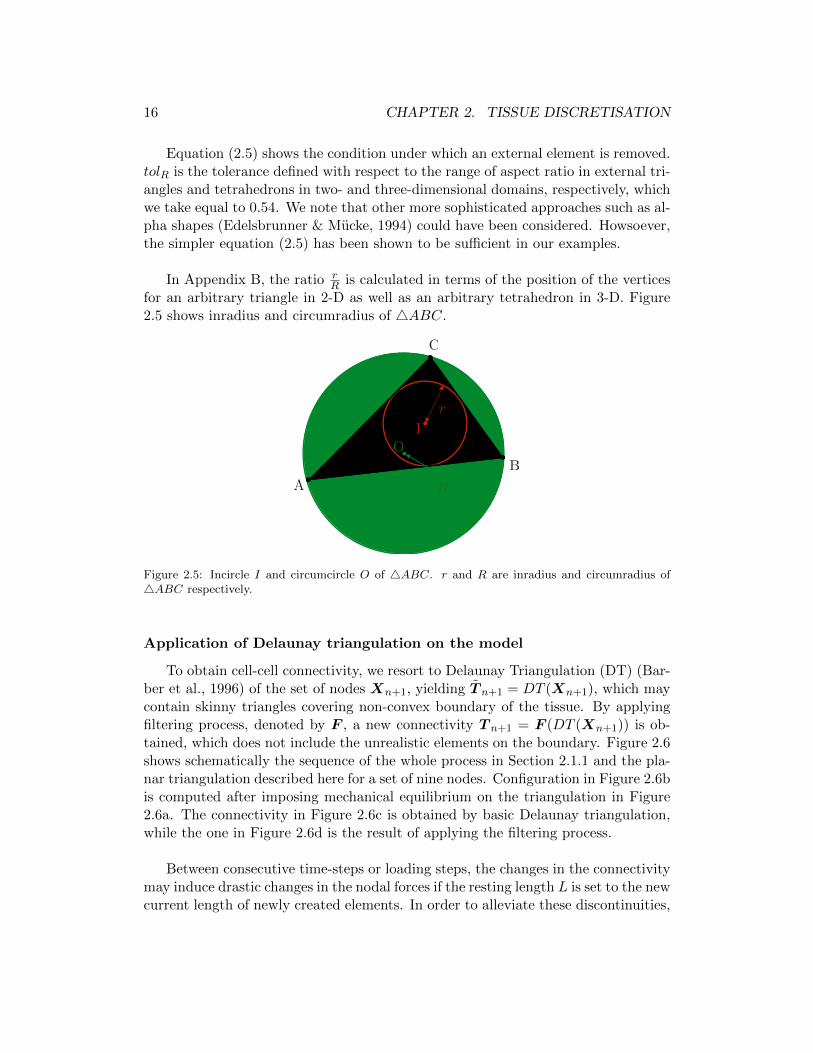
for an arbitrary triangle in 2-D as well as an arbitrary tetrahedron in 3-D. Figure2.5 shows inradius and circumradius of 4ABC.
r
R
C
B
A
IO
Figure 2.5: Incircle I and circumcircle O of 4ABC. r and R are inradius and circumradius of4ABC respectively.
Application of Delaunay triangulation on the model
To obtain cell-cell connectivity, we resort to Delaunay Triangulation (DT) (Bar-ber et al., 1996) of the set of nodes Xn+1, yielding T n+1 = DT (Xn+1), which maycontain skinny triangles covering non-convex boundary of the tissue. By applyingfiltering process, denoted by F , a new connectivity T n+1 = F (DT (Xn+1)) is ob-tained, which does not include the unrealistic elements on the boundary. Figure 2.6shows schematically the sequence of the whole process in Section 2.1.1 and the pla-nar triangulation described here for a set of nine nodes. Configuration in Figure 2.6bis computed after imposing mechanical equilibrium on the triangulation in Figure2.6a. The connectivity in Figure 2.6c is obtained by basic Delaunay triangulation,while the one in Figure 2.6d is the result of applying the filtering process.
Between consecutive time-steps or loading steps, the changes in the connectivitymay induce drastic changes in the nodal forces if the resting length L is set to the newcurrent length of newly created elements. In order to alleviate these discontinuities,

2.1. CELL-CENTRED MODEL 17
equilibrium Delaunay filtering
nT
nX
n+1T~
n+1T
displacement
n+1X~
nT
n+1X
nT
n+1X n+1X
(a) (b) (c) (d) (e)
equilibrium Delaunay filtering
nT
nX
n+1T~
n+1T
displacement
n+1X~
nT
n+1X
nT
n+1X n+1X
(a) (b) (c) (d) (e)
Xn
T n
Xn+1
T n T n+1 T n+1
Xn+1 Xn+1
(a) (d)(c)(b)(a) (b) (c) (d)
equilibrium DT F (DT )
Figure 2.6: Schematic of computational process for retrieving nodal positions an connectivityXn+1,T n+1 from the same quantities at time tn. (a)→(b): computation of new positions Xn+1
from mechanical equilibrium. (b)→(c): computation of new connectivity T n+1 from Delaunaytriangulation. (c)→(d): trimming of Delaunay connectivity T n+1, resulting in a not necessarilyconvex boundary of the cell-centred network T n+1.
a specific remodelling algorithm that defines a nodal based resting length tensor ispresented next.
2.1.3 Remodelling of cell-centred model: L-tensor method
The nodal forces are based on the elastic strain function defined in Section2.1.1, which depends on the current l and reference length L, which so far has beenconsidered constant. However, due to the redefinition of the cell-cell connectivity,detailed in Section 2.1.2, it may well be that the element ij exists at time tn+1 butnot at time tn. For this reason, we compute a nodal active length tensor, Li, whichwill allow us to compute the resting length along an arbitrary direction nj as
Lij = nj · Linj . (2.6)
This relation reveals that Li may be interpreted as a strain tensor, where thequantity nj · Linj corresponds to the stretching along nj . Since the skew part ofLi does not affect the value of Lij in equation (2.6), and in order to keep similaritybetween Li and a deformation tensor, we will assume that Li is symmetric.
It is clear that for a given node i, the existance of an active length tensor Li
satisfying exactly relationship in equation (2.6) for all current cell–cell connectionsij may not be possible. Therefore, the tensor Li is computed by minimising thefollowing quadratic error function:
EiL =1
2
Si∑
j=1
∥∥Linj − Lijnj∥∥2. (2.7)
We note that, in view of equation (2.6), we could alternatively aim to minimise
the error function EiL = 12
∑Si
j=1
∥∥∥njTLinj − Lij∥∥∥
2. We have not done so for reasons
that will be explained below, when commenting the uniqueness of the minimiser.

18 CHAPTER 2. TISSUE DISCRETISATION
Due to the symmetry of tensor Li, we will right this tensor in the forms
Li2D = Lxx, Lyy, LzzT ,Li3D = Lxx, Lyy, Lzz, Lxy, Lxz, LyzT ,
so that Linj = NjLi, with Nj a matrix that contains the components of the unitvector nj . Then, the error EiL reads
EiL =1
2
Si∑
j=1
∥∥NjLi − Lijnj∥∥2,
and its derivative with respect to each one of the components of Li gives rise to thesystem of equations
ALi = b (2.8)
with
A =Si∑
j=1
NjTNj , b =Si∑
j=1
LijNjTnj .
The error measure EiL in equation (2.7) is a quadratic function that has a uniqueminimiser as far as the vectors nj span Rnsd , with nsd the number of space dimen-sions. Appendix C gives a proof of this fact. The symmetry of Li is not required inthe proof of uniqueness, which opens the possibility for considering a non-symmetrictensor Li. However, in this case, the system of equations in (2.8) contains more un-knowns, wihtout any qualitative improvement in the retrieved active lengtheningLij = nj · Linj . Furthermore, and although we do not prove it here, we point outthat other alternative error measures as the function EiL mentioned above wouldnot guarantee a unique minimiser, even if the vectors nj span Rnsd .
The computation of the nodal strain tensor through equation (2.8) allows us tocompute the resting lengths along the directions of the new elements when connec-tivity changes occur. We emphasise that this system of equations is solved duringthe remodelling process after each time-step, while keeping the nodal positions fixed.
2.1.4 Cell-centred model for curved monolayers
Triangulation of curved manifolds
To obtain the new triangulation at step (c) in Figure 2.6 for a curved tissue,including the filtering process of Delaunay triangulation, we resort to a non-lineardimensionality reduction method (NLDR) to embed the three-dimensional scattered

2.1. CELL-CENTRED MODEL 19
set of points describing the cell centres in a two-dimensional embedding. In general,NLDR techniques suppose that the input high-dimensional point-set either lies onor is close enough to a low dimensional manifold (in our case a two-dimensionalmanifold) that also is an open set (see for instance Carreira-Perpinan (1997), Lee &Verleysen (2007), and Maaten et al. (2009)).
Here we use a robust and efficient variation of the well known local linear embed-ding (LLE) technique (Roweis & Saul, 2000), that is the modified local linear embed-ding (MLLE) (Zhang & Wang, 2007)). LLE-based methods assume that each pointof the manifold can be locally approximated by a linear combination of its k-nearestneighbours (k−nn). LLE ignores metric information producing low-dimensional em-bedding of unit covariance through a minimisation process that involves eigenvaluedecomposition of sparse matrices. The reader is referred to Roweis & Saul (2003),Roweis & Saul (2000) and Zhang & Wang (2007) for full details, and to Millan etal. (2013) for a concise description and performance comparison with other NLDRmethods in the manipulation of point-set surfaces.
As we have mentioned, a remarkable feature of LLE-based methods is the lack ofa clear metric relationship between the low-dimensional embedding and the originaldata (see Figure 2.7b). In the problems tackled in this work this is not problematic ascan be noticed in Figure 2.7c, even when the input point-set describes an elongatedsurface as that shown in Figure 2.7a. Finally, the resulting Delaunay triangulationfrom the filtering process is attached to the input point-set surface as depicted inFigure 2.7d.
Mechanical equilibrium in curved manifolds
Mechanical equilibrium in a monolayer of cell centres, on a curved manifoldand connected by bar elements is obtained by minimisation of the elastic strainfunction in equation (2.1), which is written in terms of its spatial coordinates (notthe two-dimensional embedding).
Depending on the boundary condition applied on a curved network, and due tothe absence of bending elasticity in the network, minimisation of the global elasticstrain in equation (2.1) may lead to multiple solutions, i.e. the equilibrium equationsin (2.2) yield multiple solutions for Xn+1 = x1
n+1,x2n+1, . . . ,x
Nnodesn+1 .
From mechanical point of view, this situation corresponds to the existence ofrigid-body modes in the network, when multiple positions of nodes correspond tothe same set of strain values along the bar elements. Figure 2.8 shows multiple rigidmodes of a curved monolayer with the indicated boundary conditions.

20 CHAPTER 2. TISSUE DISCRETISATION
(a) (b)
(c)(d)
−150
15
−50
0
50−5
05
−0.05 0 0.05
−0.05
0
0.05
−0.05 0 0.05
−0.05
0
0.05
z
y
x
1
2
1
2
−150
15
−50
0
50−5
05
z
y
x
(c)
(b)(a)
(d)
Figure 2.7: (a) Arbitrary point set configuration from a proof of concept example in 3-D. (b)Two-dimensional embedding obtained by using MLLE (Zhang & Wang, 2007)(k-nn=8). The lackof metric related to the input data, that is, different distances between points in the real andmapped domain, and its unit covariance (mapped points are distributed on a squared region) areapparent from the picture. (c) Two-dimensional embedding nodes and connectivity after applyingthe filtering described in Section 2.1.2. (d) Three-dimensional initial point set configuration withresulting connectivity. The colour-map, which indicates the identifier of each sample of the pointset, is provided for visual inspection.
In mathematical terms, this situation occurs when the determinant of the Jaco-bian of the system (see Appendix E) is close to zero
|K| ' 0. (2.9)
Therefore, K has at least one eigenvector κ with eigenvalue close to 0 (which wecall 0-eigenmodes) and is thus semi-positive-definite.
In order to obtain a positive-definite Jacobian matrix, and thus a system ofequations with a unique solution, we here propose a method to penalise solutionsu which include eigenvectors κ, so that the elastic strain function in equation (2.1)will be minimised by a unique u. In order to penalise 0-eigenmodes of K, we resort

2.1. CELL-CENTRED MODEL 21
x
y
z
z = 0
z = 5
Figure 2.8: Top: monolayer with half-cylinder geometry. The nodes at the plane z = 0 areconstrained to remain in the plane, while the nodes at the other base of the half-cylinder areconstrained to remain in plane z = 5. Bottom: multiple rigid modes of the monolayer with half-cylinder geometry.
to minimise the function Wc(x) where
Wc(x) = WD(x) +pr2
neig∑
l=1
(κlTu(x)
)2, (2.10)
where neig is the number of eigenvectors κ whose eigenvalue is smaller than numer-ical precision δ which can be chosen sufficiently close to 0, and pr is a penalisationfactor.
Minimisation of the strain energy in equation (2.10) will lead to
Kcu = gc,
where
Kc = K + pr
neig∑
l=1
κl ⊗ κlT ,
gc = g + pr
neig∑
l=1
(κlTu)κl.
(2.11)
Clearly, Kc is positive-definite, and thus the use of the residual in equation (2.11)will have unique solution for gc = 0. Eigenvectors κ are obtained by MATLABfunction eig, which is able to compute the eigenvectors as well as the correspondingeigenvalues of arbitrary square matrices (in our case stiffness matrix K).
22 CHAPTER 2. TISSUE DISCRETISATION
2.1.5 Cells boundary
Voronoi diagram
By definition, a Voronoi diagram is a partitioning of the domain into regionsbased on distance to a predefined set of nodes, and for each node there is a cor-responding region consisting of all points closer to that node than to any other.The Voronoi diagram of a set of points is dual to its Delaunay triangulation: eachVoronoi face is perpendicular to the connecting line of the Delaunay triangulation,and splits it in half (Barber et al., 1996). In Appendix D the tessellation of theVoronoi diagram from the Delaunay triangulation of the set of points is calculated.
In two-dimensional Euclidean space each Voronoi region forms a convex polygonand in three-dimensional Euclidean space each Vornoi region forms a convex polytopresulting from intersection of planes of perpendicular bisectors.
Application of Voronoi diagram to construct cells boundary
In this section, we resort to standard Voronoi tessellation algorithm of nodesXn+1 to represent the cells boundaries. However, the use of standard Voronoialgorithm yields regions with unbounded subdomains closing at infinity. To resolvethis issue, a set of off-set nodes were added to the original set of nodes at theboundary of the filtered Delaunay triangulation. In the next points (a), (b) and(c) we will explain how off-set nodes are defined for the two- and three-dimensionalnodal configurations.
(a) In two-dimensional nodal configurations, each boundary node xi is connectedto two boundary elements, let us say ij and ik. We define the position of twooff-set nodes xi,ijoff−set and xi,ikoff−set at a constant distance ε from node xi and
along the external normal to each element, represented by nij and nik (seeFigure 2.10c).
xi,ijoff−set = xi + εnij ,
xi,ikoff−set = xi + εnik.(2.12)
(b) In three-dimensional nodal configurations representing cellular aggregates, eachnode xi at the boundary belongs to nT i boundary triangles representing nT i
planes in space. We add nT i off-set nodes at distance ε to node xi and along theexternal normal to each of the nT i planes. The set T i contains all the trianglesT i,m including node xi and m = 1, 2, . . . , nT i .
xi,Ti,m
off−set = xi + εnTi,m. (2.13)

2.1. CELL-CENTRED MODEL 23
(c) In three-dimensional nodal configurations representing cellular monolayers, off-set nodes are performed at two stages:
(c1) In-plane off-set nodes are added for each node at the boundary of themonolayer (see Figure 2.9). Having elements ij and ik as boundary ele-ments being connected to node xi and corresponding to triangles T i,p andT i,q, off-set nodes xi,ij and xi,ik are defined at the constant distance ε tonode xi and along external normals nij,‖T
i,pand nik,‖T
i,qto the elements
ij and ik, respectively. Vectors nij,‖Ti,p
and nik,‖Ti,q
represent normal toelement ij in the plane of T i,p, and normal to element ik in the plane ofT i,q, respectively.
xi,ijoff−set = xi + εnij,‖Ti,p,
xi,ikoff−set = xi + εnik,‖Ti,q.
(2.14)
(c2) A set of out-of-plane off-set nodes are constructed for the whole set ofthe nodes in the domain and at both sides of the monolayer (see Figure2.9). So for each node xi, we define nT i off-set nodes, at each side of themonolayer, in a distance ε from node xi, along the normal nT
i,mwhere
m = 1, 2, . . . , nT i .
xi,Ti,m,+
off−set = xi + εnTi,m,
xi,Ti,m,−
off−set = xi − εnT i,m .(2.15)
The Voronoi tessellation was performed taking into account Delaunay triangu-lation of the original nodes Xn+1 and the additional off-set nodes Xoff−set,n+1.The triangulation on the whole three-dimensional domain formed by Xn+1 and theoff-set nodes, DT (Xn+1,Xoff−set,n+1), ensures the formation of bounded regionsfor the original nodes in the domain. Figure 2.10a illustrates a schematic view of aset of nodes preliminary connected by Delaunay triangulation. Figure 2.10b showsthe unbounded regions created by directly applying Voronoi tessellation on a two-dimensional nodal configuration, case (a) above. Figure 2.10c indicates the off-setnodes by yellow circles, while 2.10d shows Delaunay triangulation of combinationof original and off-set nodes, as well as Voronoi tessellation of total nodal network,which after removing the unbounded regions and the off-set nodes, results in thefinal Voronoi regions of the original set of nodes (see Figure 2.10e). The off-set nodesand elements are finally removed.
In summary, the steps followed to form the Voronoi tessellation are:
1. Form off-set layer of nodes. Based on the type of the domain geometry ex-plained previously in items (a), (b) and (c), the position of off-set nodes arecomputed by either equations (2.12) and (2.13), or equations (2.14) and (2.15).
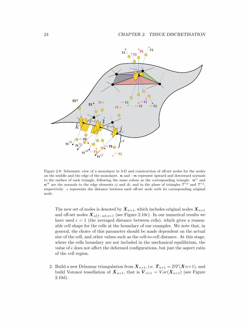
24 CHAPTER 2. TISSUE DISCRETISATION
k jiT i,q
T i,p
n
n
n
n
n
n n nn
nn n
n
n
n
n
nik
nij
nijnik
Figure 2.9: Schematic view of a monolayer in 3-D and construction of off-set nodes for the nodeson the middle and the edge of the monolayer. n and −n represent upward and downward normalsto the surface of each triangle, following the same colour as the corresponding triangle. nij andnik are the normals to the edge elements ij and ik, and in the plane of triangles T i,p and T i,q,respectively. ε represents the distance between each off-set node with its corresponding originalnode.
The new set of nodes is denoted by Xn+1, which includes original nodes Xn+1
and off-set nodes Xoff−set,n+1 (see Figure 2.10c). In our numerical results wehave used ε = 1 (the averaged distance between cells), which gives a reason-able cell shape for the cells at the boundary of our examples. We note that, ingeneral, the choice of this parameter should be made dependent on the actualsize of the cell, and other values such as the cell-to-cell distance. At this stage,where the cells boundary are not included in the mechanical equilibrium, thevalue of ε does not affect the deformed configurations, but just the aspect ratioof the cell region.
2. Build a new Delaunay triangulation from Xn+1, i.e. T n+1 = DT (Xn+1), andbuild Voronoi tessellation of Xn+1, that is V n+1 = V or(Xn+1) (see Figure2.10d).

2.2. HYBRID MODEL 25
(d)(c)
(b)(a)
(e)
T n+1
Xn+1
T n+1
T n+1
Xn+1
eV n+1
Xn+1 Xn+1
T n+1
V n+1
T n+1
Xn+1
V n+1
Voronoi
o↵-set
Voronoi o↵-setremoving
Figure 2.10: Voronoi tessellation. (a) Delaunay triangulation of original set of nodes (T n+1 =DT (Xn+1)). (b) Voronoi tessellation of original set of nodes resulting in open regions for the
nodes the boundary (V n+1 = V or(Xn+1)). (c) construct off-set nodes at the boundary of thedomain (Xn+1 = Xn+1,Xoff−set,n+1). (d) Delaunay triangulation of total nodal configuration(T n+1 = DT (Xn+1)), and obtain total Voronoi tessellation (V n+1 = V or(Xn+1)). (e) Removeoff-set nodes and elements and obtain close regions for all original nodes.
3. Remove Voronoi elements coinciding at infinity (see Figure 2.10e) and removenodes and elements at the off-set layer.
2.2 Hybrid model
So far, in the proposed model, mechanics of the tissue has been described solelyby interaction between cell centres defined by the evolution of connecting bar ele-ments. Therefore, mechanical equilibrium was obtained by minimising the elasticpotential equation (2.1), while the boundary of the cells was obtained using Voronoitessellation of the cell centres network, having no role in the mechanics of the system.
In this section, we also assign mechanics on the cells boundary, so that mechanicsof the tissue will be described by resorting to a quadratic potential along cell-cellboundaries as well as bar elements between cell centres or nodes. We will also

26 CHAPTER 2. TISSUE DISCRETISATION
focus on flat monolayers where the cell deformations along the thickness directionis assumed constant, and thus our description is restricted to the two-dimensionaltissue architectures.
While accounting for mechanics on the cells boundary, we keep the cell centresas our primary variables for establishing the equilibrium of the cell system. Thiswill require to compute the contribution of each cell boundary at the cell centres.The boundaries of the cells are defined by a set of vertices which are described interms of the position of cell centres through an interpolation procedure.
2.2.1 Vertex geometry and barycentric tessellation
We assume a tissue with flat monolayer geometry and Nnodes nodes, as de-scribed in Section 2.1, and a triangulation of the domain in Ntri triangles T I ,I = 1, 2, . . . , Ntri and ND edges. The boundary of the cells are defined by a setof connected vertices y1,y2, . . . ,yNtri, which define a tessellation of the tissue do-main into Ncells cell domains Ωi, i = 1, 2, . . . , Ncells. Note that now Ncells < Nnodes
because Ncells does not include the external nodes. We exclude boundary of the cellsat the edge of the monolayer, since the mechanical contribution of the boundary ofthese cells will be negligible in a tissue with high number of cells.
Each triangle T I is associated to vertex yI , and each interior node i is surroundedby a number of vertices which is not necessarily constant between time-steps andmay vary from cell to cell (see Figure 2.11).
yI
yJ
x ix j
I
nodes
vertices
cells
triangles
cell-centre connections
cell boundaries
Figure 2.11: Discretisation of tissue into cell centres (nodes, xi) and cells boundaries (vertices, yi).Nodal network and vertex network are outlined with continuous and dashed lines, respectively.
The position of vertex yI is given by a local parametric coordinate ξI in triangleT I . The kinematic relation between the nodal positions xi and the vetices is given

2.2. HYBRID MODEL 27
by the interpolation
yI =∑
i∈T Ipi(ξI)xi. (2.16)
Summation in equation (2.16) extends to the three nodes of triangle T I wherevertex I is located. Function pi(ξI) is the standard finite element interpolationfunction of node i in triangle T I evaluated at coordinate ξI = ξI1 ξI2:
p1(ξI) = ξI1
p2(ξI) = ξI2
p3(ξI) = 1− ξI1 − ξI2 .
Choice of tessellation
We recall that Voronoi tessellation guarantees that the cells are convex and canbe obtained by interpolation of nodes in a triangle following a Delaunay triangu-lation. However, when the nodal network is mechanically deformed, convexity ofthe cells can be violated due to length changes of the Delaunay triangulation (seeFigure 2.12), and we will avoid using Voronoi tessellation to define cells. For com-pleteness reasons though, appendices D.3 and D.4 show how the values of ξI maybe computed when the positions of the vertices correspond to Voronoi locations.
Instead, we introduce barycentric tessellation of the nodal network to definethe position of vertices, which is tantamount to considering that all parameters ξI
have a constant value ξI = 131 1. The value guarantees that the vertices are
always located at the interior of the triangles, and thus ensures that the tessellationhas no cross-overs even if the Delaunay triangulation is deformed (see Figure 2.12).We will eventually allow varying values of ξI in Section 2.2.4, where ξ-relaxation isintroduced.
2.2.2 Vertex mechanical equilibrium
To provide mechanics on cells boundary, we define an elastic strain function fromwhich the force between any two vertices is derived,
W IJV (y) =
1
2kV (εIJ)2
WV (y) =
NV∑
IJ=1
W IJV (y),
(2.17)
with kV the cell boundary stretching stiffness and εIJ = lIJ−LIJLIJ
is a scalar elastic
strain where lIJ =∥∥yI − yJ
∥∥ and LIJ are the current and reference lengths of

28 CHAPTER 2. TISSUE DISCRETISATION
xin
xjn
yIn
yJn
T J
T I
xin
xjn
yIn
yJn
T J
T I
xin+1
xjn+1
yIn+1
yJn+1
T J
T I
xin+1
xjn+1
yIn+1
yJn+1
T J
T I
(d)(c)
(b)(a)
deformation
deformation
Figure 2.12: Differences between Voronoi (top) and barycentric vertex positions (bottom) for un-deformed (left) and deformed networks (right).(a) Nodal network (in black) with Delaunay tri-angulation and vertex network (in red) with Voronoi tessellation. (b) Deformed nodal network:non-Delaunay triangulation; vertices defined by interpolation of nodes in each triangle, located atthe intersection of perpendicular bisectors of each triangle, forming a non-Voronoi vertex network.(c) Nodal network with Delaunay triangulation and vertex network with Barycentric tessellation.(d) Deformed nodal network: non-Delaunay triangulation; vertices defined by interpolation of nodesin each triangle, located at the Barycentres of each triangle, forming a barycentric vertex network.
boundary element IJ . The mechanical strain energy of the system is the sum of thecontributions of the nodal and vertex networks,
WD(x) +WV (y(x)).
The new nodal positions are found by solving the minimisation problem
x∗ = argminx
(WD(x) +WV (y(x))
), (2.18)
which may be solved in two manners:
1. as a constrained minimisation problem, where nodes xi and vertices yI areindependent but coupled through the constraint in equation (2.16), that isimposed with Lagrange multipliers.

2.2. HYBRID MODEL 29
2. by using the constraint in equation (2.16) in the expression of the objectivefunction (total strain energy) and keeping this relation in the minimisationprocess.
We choose approach (2) in order to reduce the number of unknowns, and thusthe size of the resulting system of equations. In order to deduce the expression of∂WV
∂xi, by using equation (2.17), we define first the vertex tractions as
tIJV =∂W IJ
V
∂yI= kV ε
IJ 1
LIJ lIJ(yI − yJ),
tJIV =∂W IJ
V
∂yJ= kV ε
IJ 1
LIJ lIJ(yJ − yI).
(2.19)
Therefore,
tIJV =∂W IJ
V
∂yI= −tJIV = −∂W
JIV
∂yJ. (2.20)
x i
x j
yI
yJtIJV
tJIV
I
xk
Figure 2.13: Cell boundary (highlighted polygon) corresponding to node i. Barycentric tessellationof 4ijk results to triple-junction yI . Vector tIJV represents the traction between vertices yI andyJ along the shared boundary of cells xi and xk.
The nodal residual due to contributions of the vertex network, denoted by giV ,may be then computed by using the chain rule and the kinematic relation in equation(2.16),
giV : =∂WV
∂xi=∑
IJ
(∂W IJ
V
∂yI∂yI
∂xi+∂W IJ
V
∂yJ∂yJ
∂xi
)=∑
IJ
(tIJV p
i(ξI) + tJIV pi(ξJ)
)
=∑
I∈Bipi(ξI)
∑
J∈SItIJV .
(2.21)

30 CHAPTER 2. TISSUE DISCRETISATION
In the last expression Bi denotes the set of vertices that form the boundary ofcell i, centred on xi, and SI is the set of vertices connected to vertex I. Note alsothat the last equality follows from the fact that pj(ξK) vanishes if K /∈ Bj .
Total mechanical equilibrium is then found by solving the minimisation in equa-tion (2.18), which yields,
∑
j∈SitijD +
∑
I∈Bipi(ξI)
∑
J∈SItIJV = 0, i = 1, 2, . . . , Nnodes, (2.22)
which in terms of the force contributions giD and giV reads
giD + giV = 0, i = 1, 2, . . . , Nnodes. (2.23)
The summation in the second term of equation (2.22) involves the vertex barsthat have at least one vertex on the triangles that surround node xi. Figure 2.13shows schematic view of how the boundary of each cell is defined within the tissue,and the traction vectors tIJV and tJIV .
Mechanical equilibrium of the system is obtained at cell centres (nodes) by solv-ing the set of equations in equation (2.22). As mentioned before, since this equationis non-linear with respect to the positions of the nodes, we resort to Newton-Raphsonmethod for its solution. The required linearisation of the terms in equation (2.22)is given in Appendix E.
Note that the second term in equation (2.22) arises due to the kinematic in-terpolation in equation (2.16). This term represents the nodal contribution of thevertex forces (reactions of the constraints in equation (2.16)), which is proportionalto the values of the shape functions pi(ξI). This equation shows the coupling be-tween nodal and vertex equilibrium. When vertex forces exist (kV 6= 0), nodal forcesand vertex forces are not necessarily equilibrated at nodes and vertices, respectively,that is, we may have that giD 6= 0 and
∑J∈SI t
IJV 6= 0. The latter condition is the
equilibrium equation usually imposed in purely vertex models (Alt et al., 2017). Wewill analyse the evolution of these resultants in Chapter 4.
2.2.3 Area constraint
Cell volume invariance under tissue extension is relevant when the size and thenumber of cells within the tissue is considered as constant. A two-dimensional areaconstraint will be imposed here by adding the energy term
WA =λA2
Ncells∑
m=1
(Am −Am0 )2, (2.24)

2.2. HYBRID MODEL 31
where λA is a penalisation coefficient and Am0 and Am are the initial and the currentareas of cell m, respectively. Very high values of λA may yield an ill-conditioned sys-tem of equations, while very low values may exceedingly relax the area constraint. Inour numerical examples, we used λA ≈ 5max(kD, kV ), which yielded area variationbelow 5% in all cases.
The area of cell m can be expressed in terms of its vertices by using Gausstheorem
Am =
∫
ΩmdA =
1
2
∫
∂Ωmy · n ds, (2.25)
where y is an arbitrary point on the boundary of cell m, ds is the differentialsegment of the cell boundary and n is the outward normal. Since each cell boundaryforms a polygon, we will break the integral over the whole cell boundary into Nm
line integrals. Points between vertices I and J can be obtained by using a linearinterpolation
y = qI(α)yI + qJ(α)yJ , (2.26)
with α ∈ [−1, 1] a local coordinate along the cell boundary segment IJ , and qI(α) =12(1 − α) and qJ(α) = 1
2(1 + α) the interpolation functions. By inserting equation(2.26) into equation (2.25) and noting that ds = lIJdα/2, with lIJ =
∥∥yI − yJ∥∥, we
have
Am =1
2
Nm∑
IJ∈Pm
∫ 1
−1
∑
I
qI(α)yI · nIJ lIJ
2dα =
1
2
Nm∑
IJ∈Pm
lIJ
2(yI + yJ) · nIJ , (2.27)
where Pm denotes the segments of the polygon that surround node xm (see Figure2.13). The expression above can be simplified as
Am =1
2
Nm∑
IJ∈Pm(yI × yJ).ez =
1
2
Nm∑
IJ∈PmyI · JyJ , (2.28)
where matrix J =
[0 −11 0
]= −JT is such that (yI × yJ) · ez = yI · JyJ . Finally
the total area of the whole set of Ncells cells in the tissue, AT , can be expressed as
AT =1
2
Ncells∑
m=1
∑
IJ∈PmyI · JyJ . (2.29)
The expression of the contribution in equation (2.28) is inserted in the energyterm in equation (2.24), and appended to the total elastic energy,
W = WD(x) +WV (y(x)) +WA(y(x)),
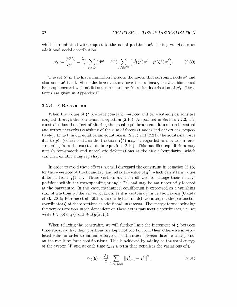
32 CHAPTER 2. TISSUE DISCRETISATION
which is minimised with respect to the nodal positions xi. This gives rise to anadditional nodal contribution,
giA :=∂WA
∂xi=λA2
∑
m∈Si(Am −Am0 )
∑
IJ∈Pm
(pi(ξI)yI − pi(ξJ)yJ
). (2.30)
The set Si in the first summation includes the nodes that surround node xi andalso node xi itself. Since the force vector above is non-linear, the Jacobian mustbe complemented with additional terms arising from the linearisation of giA. Theseterms are given in Appendix E.
2.2.4 ξ-Relaxation
When the values of ξI are kept constant, vertices and cell-centred positions arecoupled through the constraint in equation (2.16). As pointed in Section 2.2.2, thisconstraint has the effect of altering the usual equilibrium conditions in cell-centredand vertex networks (vanishing of the sum of forces at nodes and at vertices, respec-tively). In fact, in our equilibrium equations in (2.22) and (2.23), the additional forcedue to giV (which contains the tractions tIJV ) may be regarded as a reaction forcestemming from the constraints in equation (2.16). This modified equilibrium mayfurnish non-smooth and unrealistic deformations at the tissue boundaries, whichcan then exhibit a zig-zag shape.
In order to avoid these effects, we will disregard the constraint in equation (2.16)for those vertices at the boundary, and relax the value of ξI , which can attain valuesdifferent from 1
31 1. Those vertices are then allowed to change their relativepositions within the corresponding triangle T I , and may be not necessarily locatedat the barycentre. In this case, mechanical equilibrium is expressed as a vanishingsum of tractions at the vertex location, as it is customary in vertex models (Okudaet al., 2015; Perrone et al., 2016). In our hybrid model, we interpret the parametriccoordinates ξ of those vertices as additional unknowns. The energy terms includingthe vertices are now made dependent on these extra parametric coordinates, i.e. wewrite WV (y(x, ξ)) and WA(y(x, ξ)).
When relaxing the constraint, we will further limit the increment of ξ betweentime-steps, so that their positions are kept not too far from their otherwise interpo-lated value in order to minimise large discontinuities between discrete time-pointson the resulting force contributions. This is achieved by adding to the total energyof the system W and at each time tn+1 a term that penalises the variations of ξ,
Wξ(ξ) =λξ2
∑
I relaxed
∥∥ξIn+1 − ξIn∥∥2. (2.31)

2.2. HYBRID MODEL 33
By interpreting the factor λξ as a viscous coefficient ≈ η∆t , this additional term
is equivalent to a viscous-like effect, since it generates forces proportional to theincremental vertex positions (or vertex velocities).
The extension of the system with additional variables ξ also modifies the min-imisation problem in equation (2.18), which now takes the form
x∗, ξ∗ = argminx,ξ
W (x, ξ), (2.32)
with
W (x, ξ) = WD(x) +WV (y(x, ξ)) +WA(y(x, ξ)) +Wξ(ξ). (2.33)
Equilibrium is now represented by two systems of equations,
g :=
gxgy
= 0, (2.34)
with gx = ∇xW (x, ξ) and gy = ∇ξW (x, ξ). Each residual contribution in thetotal residual g is the sum of different energy contributions in (2.33), so that g =gD + gV + gA + gξ, where each term contains in turn nodal (x) and vertex (ξ)contributions,
gix : =∂W (x, ξ)
∂xi= giD + giV + giA + giξ,
gIy : =∂W (x, ξ)
∂ξi= gID + gIV + gIA + gIξ.
(2.35)
Since the nodal strain energy WD does not depend on ξI , and the penalty termWξ does not depend on nodal positions xi (see equations (2.1) and (2.31)), we havethat gID = 0 and giξ = 0. The nodal contributions giD, giV and giA have been givenrespectively in equations (2.2), (2.21) and (2.30). The vertex contributions requirethe computations of
∇ξW = ∇ξWV +∇ξWA + λξ(ξn+1 − ξn)
∂yI
∂ξI=∑
xi∈T Ixi ⊗∇pi(ξI), (2.36)
so that we have, also from equations (2.24) and (2.28),
gIV : =∂WV
∂ξI=∑
JK
∂W JKV
∂yJ∂yJ
∂ξI+∂W JK
V
∂yK∂yK
∂ξI=∑
K∈SI
∑
xi∈T I(tIKV · xi)∇pi(ξI)
gIA : = λA
Nnodes∑
m=1
(Am −Am0 )∂Am
∂ξI
gIξ : = ∇ξWξ = λξ(ξIn+1 − ξIn)
(2.37)

34 CHAPTER 2. TISSUE DISCRETISATION
with ∂yI
∂ξIgiven in equation (2.36), and
∂Am
∂ξI=
1
2
∑
KL∈Pm
(δKI
(∂yK
∂ξI
)TJyL − δLI
(∂yL
∂ξI
)TJyK
). (2.38)
The symbol δKI above is the Kronecker delta, which is equal to 1 if K = Iand 0 otherwise. We note that if we extended ξ-relaxation to the whole tissue, wecould recover standard vertex models, that is, a model where the vertices positionsare solely determined by their mechanical equilibrium: sum of forces at each vertexequal to zero. In our numerical simulations we have though just applied ξ-relaxationto specific boundaries of the domain.
2.2.5 Remodelling: Equilibrium Preserving Mapping
One of the key features of soft biological tissues is their ability to remodel, thatis, to change their neighbouring cells during growth, mobility and morphogenesis.We aim to include this feature in our hybrid model by computing a new connectivityT n+1 after each time point tn and choose a convenient value of the resting length forthe new bar elements (Mosaffa et al., 2017). Like in the purely cell-centred model,we resort to the Delaunay triangulation of the nodal network, which guarantees aminimum aspect-ratio of the resulting triangles. We also assume that these optimalaspect ratios will not be exceedingly spoiled during tissue deformation.
The redefinition of the network topology from T n to T n+1 may involve drasticchanges in the nodal and vertex equilibrium equations. Furthermore, the restinglengths Lij and LIJ are undefined for the newly created bar elements, and the com-putation of nodal resting length tensor described in Section 2.2.4 is not suitablein the present case since the number of vertices, in contrast to nodes, is not con-stant. In order to smooth mechanical transition between time-steps, we will herepresent an Equilibrium-Preserving Map that computes Lij and LIJ by minimisingthe error of the mechanical equilibrium for the new connectivity. We will considertwo approaches: a map that preserves the nodal and vertex equilibrium in a cou-pled manner (full-network mapping), and a map that preserves nodal equilibriumand vertex equilibrium independently (split-network mapping). The computationalprocess depicted in Figure 2.6 is now completed with the Equilibrium PreservingMapping (EPM) as shown in Figure 2.14.

2.2. HYBRID MODEL 35
equilibrium Delaunay filtering
nT
nX
n+1T~
n+1T
displacement
n+1X~
nT
n+1X
nT
n+1X n+1X
(a) (b) (c) (d) (e)
equilibrium Delaunay filtering
nT
nX
n+1T~
n+1T
displacement
n+1X~
nT
n+1X
nT
n+1X n+1X
(a) (b) (c) (d) (e)
Xn
T n
Xn+1
T n T n+1 T n+1
Xn+1 Xn+1
(a) (d)(c)(b)
(a) (b)
Ln Ln+1
filtering
Delaunayequilibrium and
equilibrium Delaunay filtering
nT
nX
n+1T~
n+1T
displacement
n+1X~
nT
n+1X
nT
n+1X n+1X
(a) (b) (c) (d) (e)
equilibrium Delaunay filtering
nT
nX
n+1T~
n+1T
displacement
n+1X~
nT
n+1X
nT
n+1X n+1X
(a) (b) (c) (d) (e)
Xn
T n
Xn+1
T n T n+1 T n+1
Xn+1 Xn+1
(a) (d)(c)(b)
(a) (b)
(c)
(d)
equilibrium Delaunay filtering
nT
nX
n+1T~
n+1T
displacement
n+1X~
nT
n+1X
nT
n+1X n+1X
(a) (b) (c) (d) (e)
equilibrium Delaunay filtering
nT
nX
n+1T~
n+1T
displacement
n+1X~
nT
n+1X
nT
n+1X n+1X
(a) (b) (c) (d) (e)
Xn
T n
Xn+1
T n T n+1 T n+1
Xn+1 Xn+1
(a) (d)(c)(b) (d)(c)
Ln Ln+1 Ln+1 Ln+1
mappingfiltering
Delaunayequilibrium andfilteringDelaunay
. . .
(d) (e)
Figure 2.14: Deformation and remodelling process, including the computation of the resting lengthsL∗n+1 through the Equilibrium-Preserving Map, which maintains the network connectivity and nodal
and vertex positions.
Full-network mapping
In this approach, we aim to compute a new set of resting lengths Lij and LIJ
that minimise the functional
πF (Lij , LIJ) =nodes∑
i
∥∥giD + giV + giA − ri∥∥2. (2.39)
This functional measures the error in the mechanical equilibrium considering allthe residual contributions at node i due to the cell centres (giD), the vertex network(giV ) and area constraints (giA). The latter is the value obtained from the expressionin equation (2.30), while ri is the total reaction for those nodes that have prescribeddisplacements. The residual contributions are computed as a function of nodal andvertex tractions as
giD =∑
j∈SitijD =
∑
j∈SikD
(lij
Lij− 1
)eij
giV =∑
I∈Bipi(ξI)
∑
J∈SItIJV =
∑
I∈Bipi(ξI)
∑
J∈SIkV
(lIJ
LIJ− 1
)eIJ .
(2.40)
Note that tijD and t
IJV are not defined as
∂W ijD
∂xior
∂W IJV
∂yI, but with a simpler purely
elastic law given by t = k( lL−1)e, which disregards any rheological law with evolvingresting length. These latter laws will be described in Chapter 3.
We emphasise that while computing the new resting lengths and thus the vari-ables Lij and LIJ , the nodal and vertex positions xi and yI , and also the currentlengths lij and lIJ , are all constant.
The minimisation of πF in equation (2.39) gives rise to a non-linear system ofequations in terms of the unknowns Lij and LIJ , but that is linear with respect to
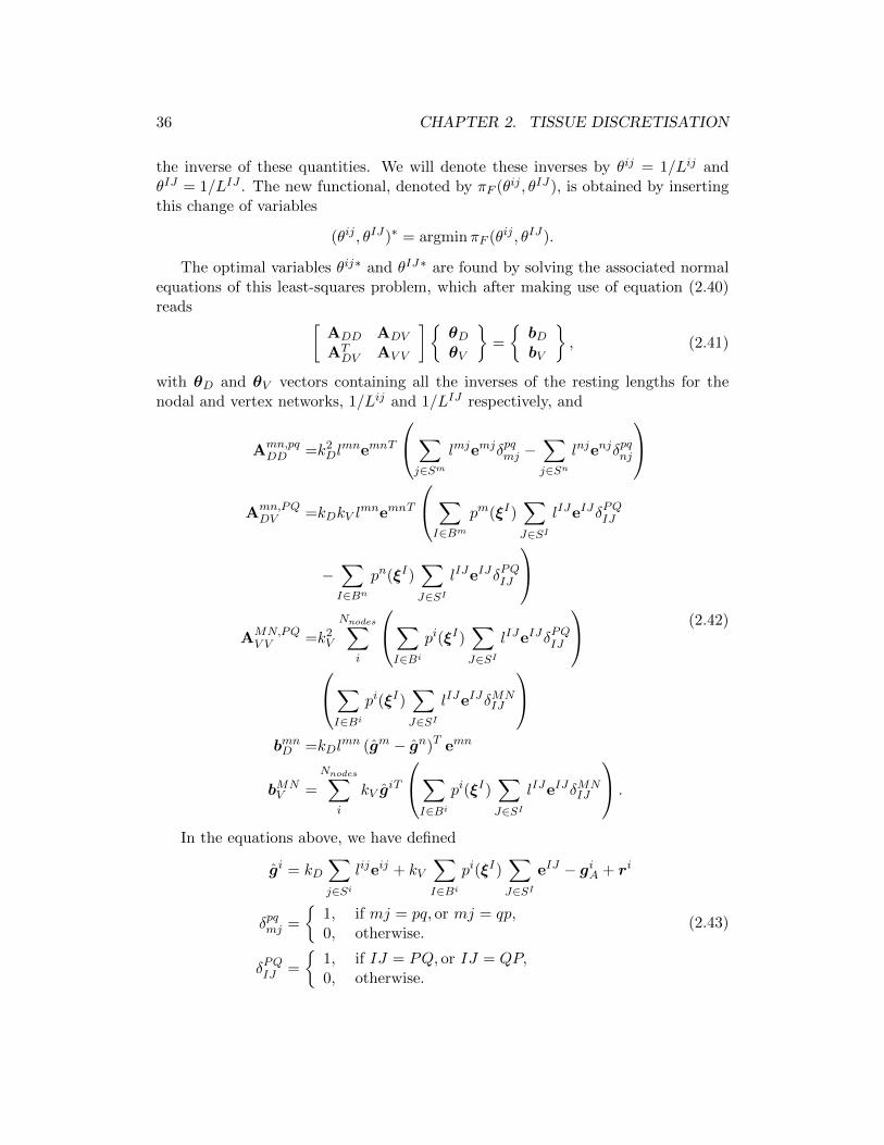
36 CHAPTER 2. TISSUE DISCRETISATION
the inverse of these quantities. We will denote these inverses by θij = 1/Lij andθIJ = 1/LIJ . The new functional, denoted by πF (θij , θIJ), is obtained by insertingthis change of variables
(θij , θIJ)∗ = argminπF (θij , θIJ).
The optimal variables θij∗ and θIJ∗ are found by solving the associated normalequations of this least-squares problem, which after making use of equation (2.40)reads
[ADD ADV
ATDV AV V
]θDθV
=
bDbV
, (2.41)
with θD and θV vectors containing all the inverses of the resting lengths for thenodal and vertex networks, 1/Lij and 1/LIJ respectively, and
Amn,pqDD =k2
DlmnemnT
∑
j∈Smlmjemjδpqmj −
∑
j∈Snlnjenjδpqnj
Amn,PQDV =kDkV l
mnemnT
∑
I∈Bmpm(ξI)
∑
J∈SIlIJeIJδPQIJ
−∑
I∈Bnpn(ξI)
∑
J∈SIlIJeIJδPQIJ
AMN,PQV V =k2
V
Nnodes∑
i
∑
I∈Bipi(ξI)
∑
J∈SIlIJeIJδPQIJ
∑
I∈Bipi(ξI)
∑
J∈SIlIJeIJδMN
IJ
bmnD =kDlmn (gm − gn)T emn
bMNV =
Nnodes∑
i
kV giT
∑
I∈Bipi(ξI)
∑
J∈SIlIJeIJδMN
IJ
.
(2.42)
In the equations above, we have defined
gi = kD∑
j∈Silijeij + kV
∑
I∈Bipi(ξI)
∑
J∈SIeIJ − giA + ri
δpqmj =
1, if mj = pq, or mj = qp,0, otherwise.
δPQIJ =
1, if IJ = PQ, or IJ = QP,0, otherwise.
(2.43)

2.2. HYBRID MODEL 37
The uniqueness of the solution of system of equations in equation (2.41), andthus the regularity of the system matrix, is in general not guaranteed, since morethan one combination of tractions in equilibrium with the reaction field may befound in some cases. This is algebraically reflected by a large condition number ofthe system matrix. For this reason, the functional is regularised by adding an extraterm,
πFλ(θij , θIJ) = πF (θij , θIJ) + λL
∑
ij
||θij − 1
lij||2+
∑
IJ
||θIJ − 1
lIJ||2 , (2.44)
with lij and lIJ the current distances between connected nodes and vertices, respec-tively. This regularisation adds a factor λL on the diagonal components and factorsλL/l
mn and λL/lMN on bmnD and bMN
V , which ensure that the system will have aunique solution for a sufficiently large value of the regularisation parameter λL. Inour numerical examples we have used λL = 10−12.
Split-network mapping
The previous approach allows us to find equilibrated tractions with a possible re-distribution of forces between the vertex and nodal networks. In some cases though,it is desirable to keep the traction contributions of the two networks split. For thisreason, we present an alternative Equilibrium-Preserving Map that aims to computethe resting lengths by considering equilibrium conditions for the nodal and vertexnetworks independently. This is achieved by minimising the functional
πS(θij , θIJ) = πD(θij) + πV (θIJ) (2.45)
with
πD(θij) =
Nnodes∑
i
||giD − riD||2
πV (θIJ) =
Nnodes∑
i
||giV − riV ||2
where riD is the contribution from the nodal network on node i before remodelling,and riV is the contribution from the vertex network to node i before remodelling.This contributions are obtained from the residual contributions before remodellingtakes place as
riD = giD,
riV = giV + giA.(2.46)

38 CHAPTER 2. TISSUE DISCRETISATION
Applying the same approach as in Section 2.2.5 to πF , the minimisation of πSyields two uncoupled systems of equations,
ADDθD = b′D
AV V θV = b′V .(2.47)
Matrices ADD and AV V are those written in equation (2.42), while the right-hand sides are now given by
b′Dmn =kDl
mn (gmD − gnD)T emn
b′VMN =
Nnodes∑
i
kV giVT
∑
I∈Bipi(ξI)
∑
J∈SIlIJeIJδMN
IJ
with
giD = kD∑
j∈Silijeij + riD,
giV = kV∑
I∈Bipi(ξI)
∑
J∈SIeIJ + riV .
Like in the previous section, a regularisation term, equal to the one used inequation (2.44) is added to the functional πS in order to ensure the regularity anduniqueness of the solution, with the same value of the regularisation parameterλL = 10−12.
The split-network approach is in fact relevant when the stresses in the nodaland vertex networks follow different patterns, and it is necessary to maintain thisdifference between the networks, such as wound healing, where the stresses aroundthe wound ring are significantly higher. Preserving stress residuals independentlyat each network guarantees the stress contrast. The full-network approach on theother hand, spoils this contrast and may transfer some of the stresses on the woundring to the nodal network. The numerical example in Chapter 4 illustrates this fact.

Chapter 3
Rheological model
Many phenomena at cellular level deal with variations in the elastic and viscousproperties of biological matter. A model should consider these features within theinhomogeneous structure of biological tissue. As a result, a cell can be deduced asa combination of viscous and elastic elements.
Within the next sections we provide description of some classical rheologicalmodels traditionally applied to describe live soft matter, as well as some recentlydeveloped models. Since rheological properties of tissues are modelled through asystem of truss elements, we restrict our description to one-dimensional rheology.For instance, a spring and a dash-pot element will display the elastic and viscouscomponents along the truss elements, respectively, which is implemented as assigningthe resulting stresses along the direction of the bar element.
3.1 Elastic model
When a material behaves elastically, the stress can be calculated directly fromthe strain, due to non-existence of path or/and time dependency. When the stressis released, the strain will become zero, so there is no permanent deformation atzero stress. All stored strain energy is released and there is no energy dissipation.
As mentioned above, the discrete material behaviour along a one-dimensionaltruss element is modelled as a spring. The behaviour here is modelled with a linearrelation between the stress σ and the elongation factor or strain ε,
σ = k ε, (3.1)
where k is the stiffness coefficient. The strain in (3.1) is defined by ε = l−L0L0
, whereL0 is the element reference length.
39

40 CHAPTER 3. RHEOLOGICAL MODEL
3.2 Kelvin-Voigt and Maxwell models
Appropriate choice and combination of a spring stiffness (elastic component) anda dash-pot viscosity, can describe the mechanical characteristics of many materials.There are two major rheological viewpoints towards modelling of visco-elasticity ofmaterials: Kelvin-Voigt and Maxwell models. In the Kelvin-Voigt model (see Figure3.1a), the two features contribute in parallel, i.e. the stress is additive and the strainis equal,
σ = σe + σv,
ε = εe = εv.(3.2)
Therefore, by having σe = kεe and σv = ηεv the total stress reads,
σ = k ε+ η ε , (3.3)
where k and η are the material stiffness and viscosity, respectively. However, inMaxwell model (see Figure 3.1b), the contribution of the two features is in serieswhich implies additive strains and equal stresses for each element,
σ = σe = σv,
ε = εe + εv,(3.4)
and the total stress reads as,
σ = k ε = η ε . (3.5)
k, "e, e
, "v, v
(a)
k, "e, e
, "v, v
(b)
Figure 3.1: Representation of (a) Kelvin-Voigt model and (b) Maxwell model.
Kelvin-Voigt model is best suited for modelling creep (strain relaxation) in astress controlled test, while Maxwell model is suitable to reproduce stress relaxationin a strain controlled test. The generalised Maxwell model (see Figure 3.2) is acombination of the two models which can be applied to both cases above and isable to fit general visco-elastic materials (Findely et al., 1989). These models canbe generalised to non-linear regimes and to continua (Holpzafel, 2007).

3.3. ACTIVE MODEL 41
k2
k1
Figure 3.2: Generalised Maxwell model
3.2.1 Implementation of Kelvin-Voigt model
Kelvin-Voigt model is implemented by using double-branched bar elements,where a fully elastic element functions in parallel with a fully viscous one.
3.2.2 Implementation of Maxwell model
By taking the first derivative of ε in equation (3.4), with respect to time t wehave,
ε = εe + εv. (3.6)
By combining equations (3.4), (3.5) and (3.12), we obtain the evolution lawbelow,
σ = k
(ε− σ
η
). (3.7)
Here, to obtain the current stress σn+1 we resort to a time-discretisation methodbased on θ scheme where σ(tn) ≈ σn+θ = (1−θ)σn+(θ)σn+1 (Wilson, 1968). Then,by assuming σ ≈ ∆σ
∆t where ∆(•) = (•)n+1 − (•)n we have,
σn+1 =
(1 +
kθ∆t
η
)−1(k∆ε+
(1 +
k∆t(θ − 1)
η
)σn
). (3.8)
3.3 Active model
Cell viscosity is not solely due to the fluid part of the cytoplasm (water) but alsodue to cell activity (Besser et al., 2011; Fung, 1993; MacKintosh & Levine, 2008;Mizuno et al., 2007). However, when retrieving characteristic viscous coefficients ofcells, there is a wide spectrum of values that have been employed, which range fromη =4.2× 10⁻³Pa s, according to the Brownian motion of molecules in embryoniccells of Drosophila melanogaster (Gregor et al., 2005), to η =105Pa s for cells atits wing imaginal disc, a value deduced from relaxation experiments (Bittig et al.,2008; Forgacs et al., 1998). While the former values are close to water viscosity(η =8.9× 10⁻⁴Pa s), the later coefficient is in fact similar to the viscosity of olive oilor ketchup-like materials. Hence, in order to shed light into the mechanisms that

42 CHAPTER 3. RHEOLOGICAL MODEL
cause the cellular response of the cell, it seems necessary to bridge the measuredviscosity and the cellular biomolecular processes. For this end, we describe next asimple phenomenologically based model that considers the observed cell viscosityas a combination of the passive cell network (Gittes & MacKintosh, 1998; Janmeyet al., 1994; MacKintosh et al., 1995) and also a consequence of active response ofthe motor proteins (MacKintosh & Levine, 2008; Mizuno et al., 2007; Morozof &Pisman, 2010).
3.3.1 Linear active model
When a set of cross-linked actin filaments in the cytoskeleton is subjected to amacroscopic strain, it stretches as a result of two combined phenomena: (i) a re-versible (elastic) deformation, and (ii) a non-reversible remodelling and lengthening.The latter is phenomenologically explained as the remodelling of the cross-links anda (de-)polymerisation process of the filaments. Figure 3.3 illustrates schematicallythese two combined effects for a pair of cross-linked polymers under a stretch pro-cess. We model these effects by allowing the resting length to vary, and becoming anadditional variable. We hypothesise that the current relative rate of resting lengthL of the combined filaments, is proportional to the elastic strain (Munoz & Albo,2013), that is
L
L= γεe, (3.9)
where εe is the elastic strain and γ is a material parameter so-called remodelling rate.It has been shown that this law can mimic the apparent visco-elastic behaviour ofcells (Munoz & Albo, 2013), and that can be used to simulate tissue fluidisation(Asadipour et al., 2016) or cell cortex response (Clement et al., 2017; Doubrovinskiet al., 2017). Note that due to the non-linear dependence of the used strain measureon the nodal or vertex positions, the viscous law includes geometrical non-linearities.Material non-linear viscous effects have been considered for instance in the contextof tissue fluidisation (Asadipour et al., 2016), or in stress relaxation (Khalilgharibiet al., 2017). By hypothesising more sophisticated laws than the one in equation(3.9), the other non-linear effects can be simulated, as it will be developed in thenext section.
The evolution law in equation (3.9) is combined with a purely linear elastic con-stitutive law in equation (2.1). This is implemented by discretising the differentialequation in (3.9) using the θ-weighted scheme presented in Section 3.2,
Ln+1 − Ln = ∆tγ(ln+θ − Ln+θ). (3.10)
In our numerical tests we have used the value θ = 0.5, which guarantees stabilityand second-order accuracy in the linear regime. The discretisation in equation

3.3. ACTIVE MODEL 43
F F
(a) (b) (c)(c)(b)(a)
L0 L > L0l = L + le
Figure 3.3: Left: Schematic of network of actin filaments connected by flexible cross-links. Right:Schematic of strain induced changes in the resting length L of a reduced system with two filamentsand a cross-link (white circle), (a) initial configuration with resting length equal to L0, (b) config-uration under an applied load, and (c) new unstrained configuration with modified resting lengthL > L0.
(3.10) allows us to write the dependence of the resting length on the current lengthvariations as
∂L
∂l=
θ∆tγ
1 + θ∆tγ. (3.11)
Due to the varying resting length, the nodal and vertex tractions along ele-ments ij and IJ , denoted by tijD and tIJV , respectively, and given in equations (2.3)and (2.19), need to be rewritten taking into account the term in equation (3.11).Therefore, with the help of the following derivation,
∂εij
∂xi=
1
L
(1− 1
L
∂L
∂l
)eij ,
∂εIJ
∂yI=
1
L
(1− 1
L
∂L
∂l
)eIJ , (3.12)
with
eij = −eji =xi − xj‖xi − xj‖ , eIJ = −eJI =
yI − yJ‖yI − yJ‖ , (3.13)
the traction forces in equations (2.3) and (2.19), then read respectively as,
tijD =∂W ij
D
∂xi= kD
εij
Lijlij
(1− ∂Lij
∂lijlij
Lij
)eij ,
tIJV =∂W IJ
V
∂yI= kV
εIJ
LIJ lIJ
(1− ∂LIJ
∂lIJlIJ
LIJ
)eIJ ,
(3.14)
where the term ∂L/∂l is given in equation (3.11). The elemental active length Lij
can be statically condensed (Munoz et al., 2013), so that only displacement degreesof freedom are globally solved.

44 CHAPTER 3. RHEOLOGICAL MODEL
Contractility
In order to include the inherent contractility that cells exert (Salbreux et al.,2012), the evolution law in (3.9) is modified as
L
L= γ(εe − εc), (3.15)
with εc a contractility parameter. This modification aims to attain a homoeostaticstrain equal to εc, at which no further modifications of the resting length take place.
The ordinary differential equation (ODE) in (3.15) is employed for the bar ele-ments of the nodal and vertex networks, and is solved together with the non-linearequations in (2.32). In fact, the evolution law is taken into account by first discreti-sation in time of the ODE in (3.15) with the θ-weighted scheme, presented in Section3.2. By using the strain definition εe = (l−L)/L, the discretisation of (3.15) yields,
Ln+1 − Ln = ∆tγ(ln+θ − Ln+θ − εcLn+θ). (3.16)
By inserting the θ-wighted scheme, the discretisation in (3.16) yields
∂L
∂l=
θ∆tγ
1 + θ∆tγ(1 + εc), (3.17)
which replaces the expression in equation (3.14).
3.3.2 Non-linear active model (power law)
Experimental tests on stress relaxation in monolayers show a trend of the stressesaccording to Khalilgharibi et al. (2017)
σ = At−α +B. (3.18)
This contradicts the standard Maxwell model using linear stress and viscousconstitutive laws introduced in (3.5), which as deduced next, exhibit a purely expo-nential evolution. The kinematic condition, where the total applied strain remainsconstant, ε = 0, allows us to write equation (3.12) as
εe + εv = 0. (3.19)
In this condition, the solution of σ in equation (3.7) has the form
σ = σ0e−tk/η. (3.20)

3.3. ACTIVE MODEL 45
To conciliate the experimental evolution of the stress σ, introduced above, witha linear elastic law where
σ = k
(l
L− 1
), (3.21)
we account for a variable resting length L, and a constant current length l as itis implied by kinematic condition (3.19). Combining the experimental trend intro-duced in equation (3.18) with linear elastic law in (3.21), the evolution of restinglength L reads as
L =kl
At−t +B + k. (3.22)
The time derivative L may be expressed in terms of L, yielding
L =αL2
klAt−α−1 =
αL2
klA
[1
A
(kl
L−B − k
)]1+1/α
= αL2
l
(k
A
)1/α(ε− B
k
)1+1/α
.
(3.23)
This evolution law may be written as
L
L=
γ
ε+ 1(ε− εc)n, (3.24)
where εc = B/k is the cell contractility (we have that L = 0 when ε = εc),γ = α(k/A)1/α is a remodelling rate, and n = 1 + 1
α . This law is a non-linearextension of the previous evolution law in (3.15), which is developed here in orderto simulate more sophisticated relaxation evolution of monolayers. In Chapter 4 wewill numerically verify that the resulting evolution law matches the observed powerlaw.


Chapter 4
Numerical Results
The methodology introduced in Chapters 2 and 3 has been implemented in MAT-LAB R2013a and MATLAB R2015b. For illustrative two- and three-dimensionalproblems, the post-processing has been completed using ParaView 4.1.0.
4.1 Extension of cell-centred networks
In this section we focus on simulation of extension of two- and three-dimensionalcellular aggregates. Since non-linear mechanical response is relevant in soft tissues,we will provide a comparison of mechanical response, between tissues with andwithout dynamic topology. We will then show how topological changes can triggernon-linear response in tissues modelled as a cell-centre nodal network with solelyelastic elements.
Two-dimensional network
A network of 45 nodes configured in two-dimensional space and forming aninitially uniform rectangle (see Figure 4.1a), is subjected to a longitudinal tractionby exerting prescribed forces along the long axis of the rectangle, following a stepfunction spanned 80 time-steps.
The coordinates of the nodes at one end of the rectangle have been fixed, expe-riencing a reaction force against the prescribed force exerted uniformly to the nodeson the other parallel end.
Three-dimensional network
A network of 225 nodes configured in three-dimensional space and initially form-ing a uniform cube (see Figure 4.1c), undergoes a purely elastic longitudinal tractionby exerting a prescribed force along the long axis of the cube, following a step func-tion spanned 80 time-steps.
47

48 CHAPTER 4. NUMERICAL RESULTS
Like in the two-dimensional case, the coordinates of the nodes at one end ofthe cube have been fixed, experiencing a reaction force against the prescribed forceexerted uniformly to the nodes on the other parallel end.
At each time-step, Newton-Raphson method has been employed to find the newequilibrated coordinates of the nodes. Then, the connectivity of the nodes has beenupdated by a Delaunay triangulation function. Finally, for visualisation purposesonly, the Voronoi tessellation function has been employed to update the Voronoivertices, at each time-step. The software package Qhull (Barber et al., 1996) hasbeen used to generate the connectivity of Voronoi cells in the three-dimensional net-work. The correction methods explained in Sections 2.1.2 and 2.1.5, for eliminatingunrealistic Delaunay vertices on concave edges and building closed Voronoi cells,have been also exploited at each time-step.
(d)
(c)
(b)
(a)
Figure 4.1: Graphical representation of (a) initial configuration of sample model in 2-D, (b) finalconfiguration (equilibrated) of two-dimensional sample under longitudinal traction, (c) initial con-figuration of sample model in 3-D, and (d) final configuration (equilibrated) of three-dimensionalsample model under longitudinal traction– Thin flashes represent uniform load on all nodes at thecorresponding face of the networks, while thick flashes represent the reaction force on the nodes onthe opposite end.
Figure 4.2a and 4.2b show plots of average displacement of those nodes experi-encing a linearly increasing external force for two networks of 45 nodes in 2-D and225 nodes in 3-D, and over a number of time-steps n = 80, under two conditions: 1)dynamic topology (connectivities updated by Delaunay triangulation at each time-step) and 2) frozen topology where initial connectivity is preserved throughout the
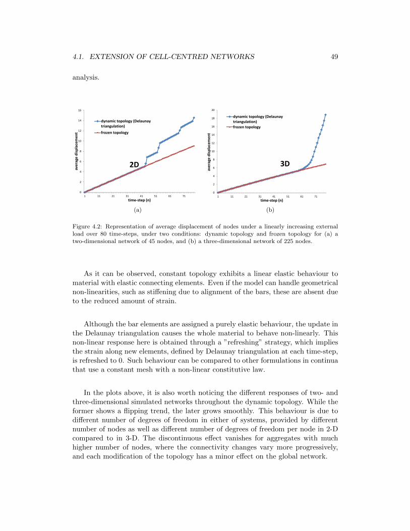
4.1. EXTENSION OF CELL-CENTRED NETWORKS 49
analysis.
0
2
4
6
8
10
12
14
16
1 11 21 31 41 51 61 71
ave
rage
dis
pla
cem
en
t
time-step (n)
2D
dynamic topology (Delaunaytriangulation)
frozen topology
(a)
0
2
4
6
8
10
12
14
16
18
20
1 11 21 31 41 51 61 71
ave
rage
dis
pla
cem
en
t
time-step (n)
3D
dynamic topology (Delaunaytriangulation)
frozen topology
(b)
Figure 4.2: Representation of average displacement of nodes under a linearly increasing externalload over 80 time-steps, under two conditions: dynamic topology and frozen topology for (a) atwo-dimensional network of 45 nodes, and (b) a three-dimensional network of 225 nodes.
As it can be observed, constant topology exhibits a linear elastic behaviour tomaterial with elastic connecting elements. Even if the model can handle geometricalnon-linearities, such as stiffening due to alignment of the bars, these are absent dueto the reduced amount of strain.
Although the bar elements are assigned a purely elastic behaviour, the update inthe Delaunay triangulation causes the whole material to behave non-linearly. Thisnon-linear response here is obtained through a ”refreshing” strategy, which impliesthe strain along new elements, defined by Delaunay triangulation at each time-step,is refreshed to 0. Such behaviour can be compared to other formulations in continuathat use a constant mesh with a non-linear constitutive law.
In the plots above, it is also worth noticing the different responses of two- andthree-dimensional simulated networks throughout the dynamic topology. While theformer shows a flipping trend, the later grows smoothly. This behaviour is due todifferent number of degrees of freedom in either of systems, provided by differentnumber of nodes as well as different number of degrees of freedom per node in 2-Dcompared to in 3-D. The discontinuous effect vanishes for aggregates with muchhigher number of nodes, where the connectivity changes vary more progressively,and each modification of the topology has a minor effect on the global network.

50 CHAPTER 4. NUMERICAL RESULTS
4.2 Active rheology in flat monolayers
In order to test the effects of the connectivity changes and also the active rhe-ological law, respectively described in Sections 2.1.2 and 3.3.1, we have simulatedthe stretching of a flat square monolayer with dimensions (Lx, Ly) = (11, 10), andsubjected to an increasing displacement ux, 0 ≤ ux ≤ 20 at the boundary X = 11,with the boundary X = 0 fixed (see Figure 4.3).
u = 0
z
y
x
ux 6= 0
uy = uz = 0
Figure 4.3: Example of flat monolayer. Top: initial geometry; Bottom: deformed geometry.
We have analysed the following two material models:
M1: γ = 0; Pure elastic material with k = 0.8.

4.2. ACTIVE RHEOLOGY IN FLAT MONOLAYERS 51
M2: γ = 0.01; Elastic material with k = 0.8 and evolving resting length L.
We have measured the sum of all the reactions along direction x for the nodesthat are initially at the boundary X = 11. The evolution of this sum, denoted byRTOT , is plotted in Figures 4.4a-b for the two material choices M1 and M2. Wehave also tested the effect of allowing cell-cell remodelling. When remodelling isallowed, we have in turn implemented two possible regimes: with stress relaxationand with no stress relaxation, which corresponds to update the resting length of thenew elements according to the expressions in Table 4.1.
0 5 10 15 200
0.5
1
1.5
2
2.5
uz
RT
OT
No RemodellingRemodellig(x)Rem + Relax(+)
(a)
0 5 10 15 200
0.1
0.2
0.3
0.4
0.5
0.6
0.7
0.8
uz
RT
OT
(b)
Figure 4.4: Total reaction RTOT at the boundary with increasing imposed displacements for the flatmonolayer. (a) Purely elastic model, (b) rheological model with active lengthening. The symbols(×) and (+) indicate the number of connectivity changes per time-step for the two simulations withremodelling.
It can be drawn from the trends of the curves in Figure 4.4 that the stressrelaxation does not have a strong effect on the total reaction, while the remodellingrate γ does have an impact in the non-linear response, introducing by itself anapparent stress relaxation. Figures 4.4a-b also indicate, with the symbols × (norelaxation) and + (with relaxation), the number of connectivity changes that takeplace during the simulation for the cases when remodelling is activated. The heightof the symbol corresponds to the number of connectivity changes divided by 10 foreach time-step. It is clear that the jumps of the response are directly correlated withthe changes of neighbours between cells. Since these are in general independent ofthe relaxation regime of the remodelling, it can be inferred that the relaxation ofRTOT is mostly due to these new connections, which have a stronger contributionon the minimisation of the stored elastic energy than the reduction of the stretchingonto the new directions when relaxation is allowed.
In order to demonstrate the equivalence between the active rheological model
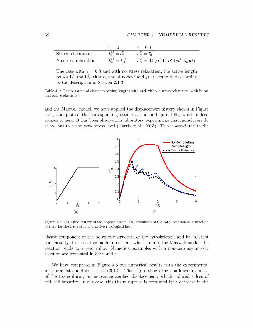
52 CHAPTER 4. NUMERICAL RESULTS
γ = 0 γ = 0.8
Stress relaxation: Lijn = lijn Lijn = lij0
No stress relaxation: Lijn = Lij0 Lijn = 0.5(ni ·Linni+nj ·Ljnnj)
The case with γ = 0.8 and with no stress relaxation, the active lengthtensor Lin and Ljn (time tn and at nodes i and j) are computed accordingto the description in Section 2.1.3
Table 4.1: Computation of elements resting lengths with and without stress relaxation, with linearand active elasticity.
and the Maxwell model, we have applied the displacement history shown in Figure4.5a, and plotted the corresponding total reaction in Figure 4.5b, which indeedrelaxes to zero. It has been observed in laboratory experiments that monolayers dorelax, but to a non-zero stress level (Harris et al., 2013). This is associated to the
0 1 2 3 40
5
10
15
20
t(s)
u z (t)
(a)
0 1 2 3 40
0.1
0.2
0.3
0.4
0.5
0.6
0.7
0.8
t(s)
RT
OT
No RemodellingRemodellig(x)Rem + Relax(+)
(b)
Figure 4.5: (a) Time history of the applied strain. (b) Evolution of the total reaction as a functionof time for the flat tissue and active rheological law.
elastic component of the polymeric structure of the cytoskeleton, and its inherentcontractility. In the active model used here, which mimics the Maxwell model, thereaction tends to a zero value. Numerical examples with a non-zero asymptoticreaction are presented in Section 4.6.
We have compared in Figure 4.6 our numerical results with the experimentalmeasurements in Harris et al. (2012). This figure shows the non-linear responseof the tissue during an increasing applied displacement, which induced a loss ofcell–cell integrity. In our case, this tissue rupture is presented by a decrease in the

4.3. ACTIVE RHEOLOGY IN CURVED MONOLAYERS 53
number of cell–cell connectivities. The trends of the two curves agree qualitativelyup to the measured experimental extension. Due to the adopted linear elastic model,our simulations do not capture the initial stiffening of the material. This may berecovered by modifying the quadratic potential in (2.1).
0 20 40 60 80 1000
1
2
3
4
5
6
7
Extension(%)
Str
ess(
kPa)
RemodellingHarris et al.(2012)
Figure 4.6: Comparison between the averaged stress value in the experimental results (Harris etal., 2012)
4.3 Active rheology in curved monolayers
We have tested a curved monolayer that has the shape of half a cylinder, with theaxis on the x direction, and with the same number of nodes and similar dimensions:the projected area occupies the same domain D = (X,Y )‖0 ≤ X ≤ 11, 0 ≤Y ≤ 10 (see Figure 4.7). The monolayer is stretched along direction x, up to thedisplacement ux = 20.
The same material models and the mapping of the surface described in Section2.1.4 has been employed in order to apply the Delaunay triangulation. Figure 4.8shows the evolution of the total reaction RTOT and the number of connectivitychanges. Similarly to the previous case, the trend of the curves is hardly affected bythe update of the active length. However, in the three-dimensional case, the effectof remodelling has a more acute effect on the reduction of the total reaction thanin the two-dimensional case, although this effect is only observed for larger imposeddisplacements.
The reduction of RTOT may be attributed to two contributions. First, the sidesX = 0 and X = 11 are fixed on the y − z plane, and since Delaunay triangulationminimises the aspect ratio of the resulting triangles, no elongated triangles can be

54 CHAPTER 4. NUMERICAL RESULTS
u = 0
ux 6= 0
uy = uz = 0
zy
x
Figure 4.7: Example of curved monolayer. Top: initial geometry. Bottom: deformed geometry
created. As a result, larger cells are built at the middle of the monolayer. Second,and although the number of cells is constant, these are intercalated as the stretchingprocess takes place: new connections are being created transversally to the stretchingdirection (y axis), which replace bars aligned on the x direction. We recognisethat the first contribution is unrealistic. To resolve this issue, certain kinematicconstraints should be added to the model in order to preserve the total volume ofeach cell. Such a constraint has been introduced in Section 2.2.3 for two-dimensional

4.4. EXTENSION OF SQUARE TISSUE EMPLOYING HYBRID MODEL 55
0 5 10 15 200
0.5
1
1.5
2
2.5
uz
RT
OT
No RemodellingRemodellig(x)Rem + Relax(+)
(a)
0 5 10 15 200
0.1
0.2
0.3
0.4
0.5
0.6
0.7
uz
RT
OT
(b)
Figure 4.8: Total reaction at the boundary with increasing imposed displacements for the curvedmonolayer, (a) purely elastic model, (b) rheological model with active lengthening.
hybrid model. The second contribution, the intercalation process, has been observedin real embryogenetic movements of curved monolayer such as the endoderm ofDrosophila melanogaster during germ band extension (Lecuit & Lenne, 2007). Wenotice that this effect is more pronounced in the three-dimensional case than in theflat monolayer, which restrained to remodel on a flat surface.
We also point out that the stress relaxation, due to either the active rheologicalmodel or the intercalation process, solely takes place along the direction of stretch-ing. The material thus remodels anisotropically, as it has been observed on tissuesduring cell motility (Trepat et al., 2009).
4.4 Extension of square tissue employing hybrid model
We test our methodology by extending a square domain obtained from a randomperturbation of a 10×10 grid of nodes (see Figure 4.9). The domain is formed by 81cells, and subjected to a uniform 30% extension applied within 60 time-steps. Thisis the amount of stretch used in recent experimental tests on monolayers (Harriset al., 2012), and also the approximated stretch that some in vivo tissues in lungsor mitral valves can be subjected to. We will test two situations: extension withconstant topology (evolution from (a) to (b)), and with remodelling (evolution from(a) to (c)). In the two situations we will apply the full and split approaches of theEquilibrium-Preserving Map (EPM). Since we aim to test here the effectiveness ofthe EPM, we prevent stress relaxation by using a small value of the remodelling rateγ = 10−6, which makes the analysis quasi-static. The resting lengths remain thusconstant, except when remodelling takes place.

56 CHAPTER 4. NUMERICAL RESULTS
(a)
(b)
(c)
Figure 4.9: Tissue extension. (a) Initial configuration, (b) tissue configuration at 30% extensionwithout remodelling, and (c) tissue configuration at 30% extension with remodelling. Replacedelements are marked in black in (b). Remodelled elements are marked in green.
4.4.1 Verification of EPM: fixed topology
To inquire the accuracy and effects of the EPM, we measure the horizental totalreaction at the right side as
Rx =
∫
∂Ωright
(giD + giV ) ·
10
ds, (4.1)
and the elastic energy of all the bar elements in the tissue during extension whilekeeping the topology constant. Figure 4.10 shows the evolution of the two quantitieswhen kD = 10 kV (Figures 4.10a-b) and when kD = 0.1 kV (Figures 4.10c-d). It canbe observed that in all cases the full-network and the split-network mappings givethe same values as the tests with no mapping. This fact shows that the EPM is ableto recover the same traction values as the ones when no computation of the restinglengths is applied, and that the system regularisation is not altering these lengthsor the elastic response of the tissue.

4.4. EXTENSION OF SQUARE TISSUE EMPLOYING HYBRID MODEL 57
0 10 20 30 40 50 60 70time-step
0
0.5
1
1.5
2
2.5
3
3.5
4
4.5re
acti
on
nomapfullmapsplitmap
(a)
0 10 20 30 40 50 60 70time-step
0
10
20
30
40
50
60
ener
gy
nodal network
vertex network
nomap - nodalfullmap - nodalsplitmap - nodalnomap - vertexfullmap - vertexsplitmap - vertex
(b)
0 10 20 30 40 50 60 70time-step
0
0.5
1
1.5
2
2.5
reac
tio
n
nomapfullmapsplitmap
(c)
0 10 20 30 40 50 60 70time-step
0
5
10
15
20
25
30
35
40
ener
gy
nodal network
vertex network
nomap - nodalfullmap - nodalsplitmap - nodalnomap - vertexfullmap - vertexsplitmap - vertex
(d)
Figure 4.10: Tissue formed by linear elastic elements, under 30% uniform stretch applied within60 time-steps while held at constant topology (no remodelling). Elements resting lengths, at eachtime-step, obtained by three approaches: fixed resting lengths (no network mapping), full-networkmapping and split-network mapping. (a) Total tissue reaction while kD = 10 kV , (b) potentialenergy of nodal and vertex networks while kD = 10 kV , (c) total tissue reaction while kD = 0.1 kV ,and (d) potential energy of nodal and vertex networks while kD = 0.1 kV .
4.4.2 Verification of EPM: variable topology
We now apply the same boundary conditions as in the previous tests, but al-lowing the tissue to remodel according to the Delaunay triangulation of the nodalpositions. Figure 4.11 shows the total reaction at the right end of the tissue andthe total elastic energy. We have monitored these three quantities under threeconditions: no remodelling/mapping, remodelling with full-network mapping andremodelling with split-network mapping. We have tested also two sets of materialproperties: kD = 10 kV (Figures 4.11a-b), and kD = 0.1 kV (Figures 4.11c-d). Thetotal number of remodelling events (elements that change their connectivity) is alsoplotted at each time-step, whenever this number is non-zero.
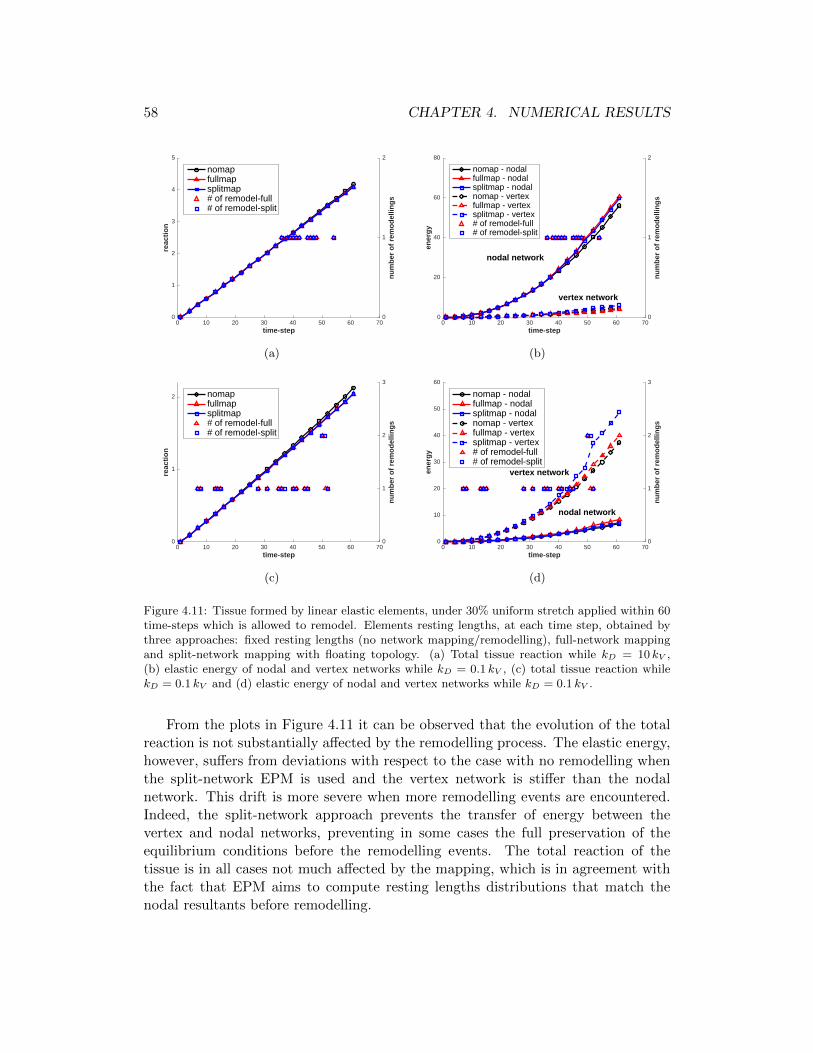
58 CHAPTER 4. NUMERICAL RESULTS
0 10 20 30 40 50 60 70time-step
0
1
2
3
4
5re
acti
on
0
1
2
nu
mb
er o
f re
mo
del
ling
s
nomapfullmapsplitmap# of remodel-full# of remodel-split
(a)
0 10 20 30 40 50 60 70time-step
0
20
40
60
80
ener
gy
nodal network
vertex network
0
1
2
nu
mb
er o
f re
mo
del
ling
s
nomap - nodalfullmap - nodalsplitmap - nodalnomap - vertexfullmap - vertexsplitmap - vertex# of remodel-full# of remodel-split
(b)
0 10 20 30 40 50 60 70time-step
0
1
2
reac
tio
n
0
1
2
3
nu
mb
er o
f re
mo
del
ling
snomapfullmapsplitmap# of remodel-full# of remodel-split
(c)
0 10 20 30 40 50 60 70time-step
0
10
20
30
40
50
60
ener
gy
nodal network
vertex network
0
1
2
3
nu
mb
er o
f re
mo
del
ling
s
nomap - nodalfullmap - nodalsplitmap - nodalnomap - vertexfullmap - vertexsplitmap - vertex# of remodel-full# of remodel-split
(d)
Figure 4.11: Tissue formed by linear elastic elements, under 30% uniform stretch applied within 60time-steps which is allowed to remodel. Elements resting lengths, at each time step, obtained bythree approaches: fixed resting lengths (no network mapping/remodelling), full-network mappingand split-network mapping with floating topology. (a) Total tissue reaction while kD = 10 kV ,(b) elastic energy of nodal and vertex networks while kD = 0.1 kV , (c) total tissue reaction whilekD = 0.1 kV and (d) elastic energy of nodal and vertex networks while kD = 0.1 kV .
From the plots in Figure 4.11 it can be observed that the evolution of the totalreaction is not substantially affected by the remodelling process. The elastic energy,however, suffers from deviations with respect to the case with no remodelling whenthe split-network EPM is used and the vertex network is stiffer than the nodalnetwork. This drift is more severe when more remodelling events are encountered.Indeed, the split-network approach prevents the transfer of energy between thevertex and nodal networks, preventing in some cases the full preservation of theequilibrium conditions before the remodelling events. The total reaction of thetissue is in all cases not much affected by the mapping, which is in agreement withthe fact that EPM aims to compute resting lengths distributions that match thenodal resultants before remodelling.

4.4. EXTENSION OF SQUARE TISSUE EMPLOYING HYBRID MODEL 59
For the two sets of material parameters, the total reaction, and thus the tissueresponse, is very much unaffected by the remodelling for the two EPM approaches.The tissue keeps the correct aspect ratio of the cells while keeping the elastic re-sponse. Although cells may use remodelling events to relax their stress state, wehere aim to independently control the stress relaxation and the remodelling events.
The computational cost of the simulations with and without remodelling, withand without area constraint, and for different combinations of the Delaunay andvertex networks is given in Table 4.2, when using the patch with 81 cells. Theremodelling affects the first iteration of each increment, but may increase the com-putational cost by 15%-45% for cases without or with area constraint. Includingthis constraint is the factor that has a major effect, which may double the com-putational time. This may be attributed, besides the computation of additionalterms in the Jacobian and residual, to the decrease of sparsity of the system matrixat each iteration due to the additional coupling that vertices include. The use ofvertex network may also noticeably increase the computational time, while due tothe methodology, assigning stiffness or not to the Delaunay has very small effectson the overall computational time.
We also note that the use of the vertex network may increase the memory re-quirement by about 60%. The present example required the use of 34.6 RAM MB,while the Delaunay only used 21.5 MB. These numbers reveal that cell-centred anal-yses are less expensive, but of course they provide no direct way to preserve cell area.
Remodelling No Remodelling
λA = 0 λA > 0 λA = 0 λA > 0
Delaunay 59 321 44 257Vertex 153 376 108 376Delaunay + Vertex 183 397 125 343
Table 4.2: Comparison of run time in seconds for different networks and remodelling combinationswhen using the stretching test with 81 cells. In the cases with remodelling, full-network mappingwas used. Split-network mapping gave very similar computational times.
4.4.3 Analysis of ξ-relaxation
Tissue stiffness against tissue total reaction and strain energy is investigated byassigning a range of values to kD kV at a constant total stiffness, kD + kV = 1,under two conditions: 1) when vertices are rigidly anchored at barycentres (ξ =131 1), and 2) when vertices are allowed to change their relative positions with

60 CHAPTER 4. NUMERICAL RESULTS
respect to the barycentres (ξ-relaxation). Figure 4.12 compares the vertex networkshown in Figure 4.9b for the two situations. The red network displays verticesanchored at barycentres, while in the green network vertices are relaxed under apenalisation factor λξ = 10−4.
In order to inspect the effect of ξ-relaxation we have analysed the reaction andenergy of mainly nodal-driven or mainly vertex-driven tissues for different values ofλξ. Figure 4.13 shows the tissue response for different values of kV ∈ [0, 1] whilekeeping kD + kV = 1, and when the tissue is subjected to an 30% extension. Figure4.13a shows that the total reaction decreases as tractions concentrate on the vertexnetwork. This reduction is steeper when vertices are relaxed (lower values of λξ).Figure 4.13b shows a faster drop in tissue total energy and a lower growth in vertexnetwork energy when ξ-relaxation is allowed, while no significant effect on the energyof the nodal network is observed.
We have also analysed the difference of our equilibrated tractions with respect tothe purely nodal and vertex equilibrium conditions: null sum of tractions at nodesand at vertices. This difference is computed as the mean value of the following nodaland vertex measures,
Ei =
∥∥∥∑
j∈Si tijD
∥∥∥∑
j∈Si∥∥∥tijD
∥∥∥, i = 1, 2, . . . , Nnodes
EI =
∥∥∑J∈SI t
IJD
∥∥∑
J∈SI∥∥tIJD
∥∥ , I = 1, 2, . . . , Ntri.
(4.2)
Figures 4.13c and 4.13d plot the means,
ED =∑
i
EiNnodes
EV =∑
I
EINtri
,
(4.3)
for the whole tissue. As expected, the nodal difference is zero when no stiffness isassigned to the vertex network (kV = 0). As kV increased, pure nodal equilibriumis increasingly violated, due to the coupling between the two networks. In mostcases, this difference is below 10%, except when vertices are fixed. Pure vertexequilibrium is more severely affected by the kinematic constraint, but the differencealso decreases rapidly as λξ decreases. It can be observed that while the positions ofthe vertices in the two networks is very similar, purely vertex equilibrium drasticallyimproves for approximately λξ < 10−2.

4.5. WOUND HEALING 61
fixed
relaxed
Figure 4.12: Deformed tissue at 30% extension. Red network represents vertices with fixed ξ. Greennetwork represents vertices when ξ-relaxation is allowed.
4.5 Wound healing
The hybrid model is tested to simulate a wound healing process in monolayers(Antunes et al., 2013). The evolution law in equation (3.15) is applied to the nodaland vertex networks with the values given in Table 4.3, which also indicates thatthe area constraint is imposed in order to mimic mechanical properties of the tissue.Topological changes in the tissue are allowed to examine the role of cell motility andcell intercalation during wound healing.
kD kV γD γV εcD εcV λA0.1 2.0 0.5 0.5 1.0 0.7 10.0
Table 4.3: Material parameters employed in the wound healing example.
Wounding and wound healing processes are simulated during the consecutivesteps below:
1. To resemble the initial condition of in vivo tissue before wounding, the mod-elled tissue is let to reach a contractile state given by the values εcD and εcV inTable 4.3 for the nodal and vertex networks respectively, and the evolution law
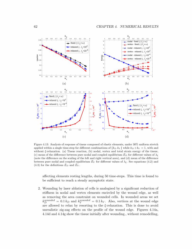
62 CHAPTER 4. NUMERICAL RESULTS
0 0.1 0.2 0.3 0.4 0.5 0.6 0.7 0.8 0.9 1K
V
0.1
0.15
0.2
0.25
0.3
0.35
0.4
0.45
reac
tio
n
fixed 9 (69=1)
relaxed 9, 69=102
relaxed 9, 69=10-4
00.10.20.30.40.50.60.70.80.91
KD
(a)
0 0.1 0.2 0.3 0.4 0.5 0.6 0.7 0.8 0.9 1K
V
0
1
2
3
4
5
6
7
8
9
En
erg
y
nodal - fixed 9 (69=1)
vertex - fixed 9 (69=1)
nodal - relaxed 9, 69=102
vertex - relaxed 9, 69=102
nodal - relaxed 9, 69=10-4
vertex - relaxed 9, 69=10-4
00.10.20.30.40.50.60.70.80.91
KD
(b)
0 0.2 0.4 0.6 0.8 1KV
0
2
4
6
8
10
12
14
ED
(%);
69=1
, 102
fixed 9 (69=1)
relaxed 9, 69=102
relaxed 9, 69=10-4
00.10.20.30.40.50.60.70.80.91
KD
0
0.5
1
1.5
2
2.5
3
3.5
4
4.5E
D(%
); 69=1
0-4
#10-4
(c)
0 0.2 0.4 0.6 0.8 1KV
30
40
50
60
70
80
90
EV
(%);
69=1
, 102
fixed 9 (69=1)
relaxed 9, 69=102
relaxed 9, 69=10-4
00.10.20.30.40.50.60.70.80.91
KD
0
1
2
3
4
5
6
EV
(%);
69=1
0-4
#10-3
(d)
Figure 4.13: Analysis of response of tissue composed of elastic elements, under 30% uniform stretchapplied within a single time-step for different combinations of kD kV while kD+kV = 1, with andwithout ξ-relaxation. (a) Tissue reaction, (b) nodal, vertex and total strain energy of the tissue,(c) mean of the difference between pure nodal and coupled equilibrium ED for different values of λξ(note the difference on the scaling of the left and right vertical axes), and (d) mean of the differencebetween pure nodal and coupled equilibrium EV for different values of λξ. See equations (4.2) and(4.3) for the definitions ED and EV .
affecting elements resting lengths, during 50 time-steps. This time is found tobe sufficient to reach a steady asymptotic state.
2. Wounding by laser ablation of cells is analogised by a significant reduction ofstiffness in nodal and vertex elements encircled by the wound edge, as wellas removing the area constraint on wounded cells. In wounded areas we setkwoundedD = 0.1 kD and kwoundedV = 0.1 kV . Also, vertices at the wound edgeare allowed to relax by resorting to the ξ-relaxation. This is done to avoidunrealistic zig-zag effects on the profile of the wound edge. Figures 4.14a,4.14d and 4.14g show the tissue initially after wounding., without remodelling,

4.5. WOUND HEALING 63
and with full- and split-network remodelling, respectively.
3. To simulate tissue eventual response to wounding, after 12 time-steps, contrac-tility on the elements of the vertex network surrounding the wound (woundring) is multiplied by 5 in order to pattern actomyosin concentration, as it hasbeen experimentally observed (Brugues et al., 2014). Figures 4.14b and 4.14eshow how the extra contractility on the wound edge results in higher tractionson the wound ring, at both non-remodelling and remodelling tissues.
4. Additional tractions on the wound ring cause the wounded area being squeezedby the cells on the wound boundary. Figures 4.14c and 4.14f show the woundclosure with and without remodelling. Including remodelling during the tissueevolution results in less cell elongation at the wound edge and allows cells torelocate during wound closure.
In the full-network strategy (Figures 4.14d-f), since the total residual of nodaland vertex networks were preserved at the nodes, the interplay of stresses in nodaland vertex networks could not preserve the higher stress in the vertex elementsat the wound ring. Instead, the split-network strategy could provide the expectedhigher stress in the elements at the wound ring. This is due to preserving nodalresidual independently in each of the networks.
We have compared the time evolution of the relative wounded area rA(t) com-puted as
rA(t) =Awounded(t)
Awounded(tablation). (4.4)
In Figure 4.15a we show this ratio for the numerical simulations and also forexperimental measurements (Brugues et al., 2014) of the same phenomenon on anablated tissue of Madin Darby kidney (MDCK) cells. It can be observed thatthe evolution of the area matches approximately the experimental values during theearly stages of the closure, but that at longer time scales, the area of the experimentalimages closes at a slower rate. This fact may reveal that the contractility of thering is not maintained constant, but that it may reduce progressively. Furtheranalysis is though required to quantify the evolution of the contraction of the tissue.Also, although intercalations away from the wound edge have been observed insome systems (Razzell et al., 2014), the impact of remodelling on wound closure inbiological systems needs to be further investigated.
In order to also evaluate the effects of using solely a nodal or a vertex network,we show in Figure 4.15b the same ratio rA for tissues where nodal or vertex stiffnesshas been reduced by 10−6. The resulting evolutions of rA reveal that the inhibitionof the Delaunay has very minor effects, while removing vertex stiffness does slow
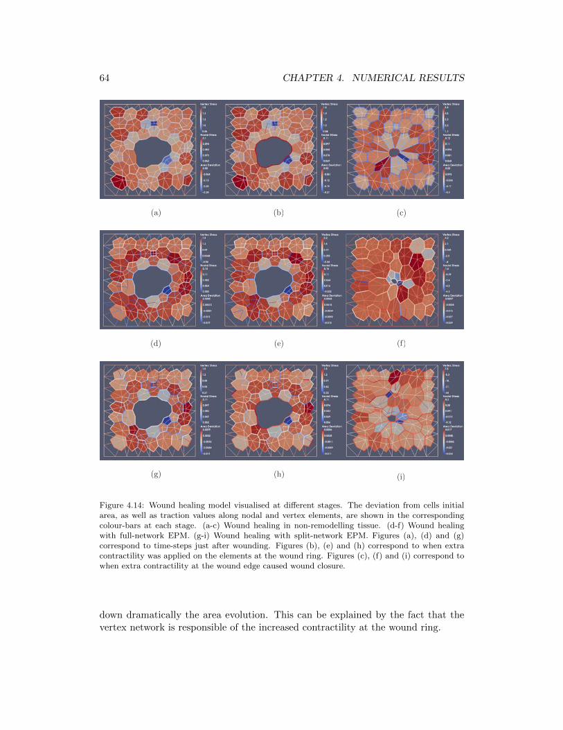
64 CHAPTER 4. NUMERICAL RESULTS
(i)(h)(g)
(f)(e)(d)
(c)(b)(a)
Figure 4.14: Wound healing model visualised at different stages. The deviation from cells initialarea, as well as traction values along nodal and vertex elements, are shown in the correspondingcolour-bars at each stage. (a-c) Wound healing in non-remodelling tissue. (d-f) Wound healingwith full-network EPM. (g-i) Wound healing with split-network EPM. Figures (a), (d) and (g)correspond to time-steps just after wounding. Figures (b), (e) and (h) correspond to when extracontractility was applied on the elements at the wound ring. Figures (c), (f) and (i) correspond towhen extra contractility at the wound edge caused wound closure.
down dramatically the area evolution. This can be explained by the fact that thevertex network is responsible of the increased contractility at the wound ring.

4.6. SHORT TIMESCALE STRESS RELAXATION IN MONOLAYERS 65
0 5 10 15 200
50
100
150
Time [min]
Rati
o A
rea, r A
[%
]
ExperimentalSplit MapFull MapNo Remod
(a)
0 5 10 15 200
20
40
60
80
100
120
140
160
180
Time [min]
Rati
o A
rea, r A
[%
]
ExperimentalSplit MapNo DelaunayNo Vertex20x20, Full Map
(b)
Figure 4.15: Time evolution of the wounded area. (a) Comparison for the three models shownin Figure 4.14 and an experimental measurement (Brugues et al., 2014), and (b) comparison forthe case with split-network mapping, inhibiting Delaunay network, inhibiting vertex network, andusing a larger mesh with 20× 20 initial nodes (361 cells).
Figure 4.15b also includes the corresponding time variation for a larger patchwith 361 cells, and a larger ablated area of 7 cells (see Figure 4.16). In this case,the peak of the area recoil is, as expected, also larger. In all cases, the slope ofthe ratio is initially similar to the experimental one, but it diverges for longer timescales. Further calibration of the contractility and its regulation is intended as afuture work.
4.6 Short timescale stress relaxation in monolayers
Stress relaxation in monolayers has been shown to be biphasic, commencing witha large amplitude fast relaxation occurring within the first approximate 5 s, followedby a small amplitude slow relaxation and reaching a plateau after almost 60 s. Ithas been shown that the first and second phases of the relaxation are dominated bya power law and an exponential response, respectively (Khalilgharibi et al., 2017).Figure 4.17a shows an experimental plot of a monolayer stress relaxation during100 s.
Based on the evolution law represented by equation (3.24), we have fitted stressrelaxation of a monolayer with a hybrid network with fixed topology, and non-linear active nodal and vertex elements for the whole 100 s, onto the experimentalcurve (see Figure 4.17b). In order to mimic the monotonous stress trend at thesecond phase, we have combined a linear elastic element in parallel with every vertexelement. The model aims to fit the power law, and as it can be observed in thefigure, this evolution is captured during the first 20 s. In the second phase, where

66 CHAPTER 4. NUMERICAL RESULTS
Figure 4.16: Wound healing simulation for a patch with 361 cells. The same parameters as thoseused in Figure 4.14 are employed here, but with 7 ablated cells, instead of 5, and for the same stageshown in Figures 4.14c, 4.14f and 4.14i. Cell colours indicate area relative variations.
cytoskeleton mechanics seems to play a major role, the numerical results are lesssatisfactory, although the trend does not depart substantially from the experimentalcurve. The value of the mechanical parameters used to fit the simulation results aregiven in Table 4.4.
We also have fitted a non-linear active single element, onto the relaxation curveduring the first phase. Figure 4.18a shows the single element evolution, fitted ontothe experimental plot during the first 20 s of the monolayer stress relaxation. Figure4.18b shows the evolution of the resting length L for the single element stress re-

4.6. SHORT TIMESCALE STRESS RELAXATION IN MONOLAYERS 67
-1 -0.5 0 0.5 1 1.5 2Log(t)
-2.95
-2.9
-2.85
-2.8
-2.75
-2.7
-2.65
-2.6
-2.55
-2.5
-2.45Lo
g(<
)
Exp
power law exponential
(a)
-1 -0.5 0 0.5 1 1.5 2Log(t)
-2.95
-2.9
-2.85
-2.8
-2.75
-2.7
-2.65
-2.6
-2.55
-2.5
-2.45
Lo
g(<
)
ExpHybrid
(b)
Figure 4.17: Biphasic stress relaxation of monolayer based on experimental results (Khalilgharibiet al., 2017). (a) The left side represents the first approximate 20 s where a power law dominatesthe relaxation, whereas the right side pertains to the rest of relaxation period, dominated by anexponential trend.(b) Stress relaxation of hybrid network with non-linear active nodal elementsand a double-branched vertex network of non-linear active and linear elastic elements combined inparallel, fitted onto the experimental trend.
-1 -0.5 0 0.5 1 1.5Log(t)
-2.9
-2.85
-2.8
-2.75
-2.7
-2.65
-2.6
-2.55
-2.5
-2.45
Lo
g(<
)
Exp1 element
(a)
-1 -0.5 0 0.5 1 1.5Log(t)
1
1.02
1.04
1.06
1.08
1.1
1.12
1.14
1.16
1.18
1.2
L
1 element
(b)
Figure 4.18: (a) Stress relaxation of simulated a non-linear active single element, against the ex-perimental plot during the first 20 s from the beginning of the relaxation period. (b) Evolution ofthe single element resting length L during the first 20 s from the beginning of the relaxation.
laxation with respect to the evolution law presented in equation (3.24) . The initialresting length has been normalised to a value of 1 unit of length.

68 CHAPTER 4. NUMERICAL RESULTS
kD γD εcD kV 1 γV 1 εcV 1 kV 2 n
1 element 0.011 1000 0.005 - - - - 6.4Hybrid 0.0049 450 0.004 0.0008 0.15 0.03 0.004 4
Table 4.4: Mechanical parameters used to fit the simulation results onto the experimental results.
Chapter 5
Conclusions
We have presented a cell-centred approach by which the non-linear response ofsoft cellular tissues, formed as either monolayer or three-dimensional aggregate, canbe simulated by modelling the relative position of cell centres and their topologicalchanges. At this stage, we have presented a method to handle mechanical responsein curved monolayers by removing the rigid-body modes of the system, as well asintroducing L-tensor method to handle the tissue topological changes by computingan appropriate resting length for the remodelled elements.
At a later stage, we have presented a hybrid approach which includes the me-chanical effect of cell boundaries in the tissues total response. This approach allowsto independently control the material properties of the cell boundaries and the cy-toplasm (cell interior). The methodology solves the mechanical equilibrium of thetwo networks in a coupled manner. The numerical results show that the approachcan reproduce relevant phenomena such as tissue extension or wound healing.
The method resorts to a rheological law that is based on an evolution law of theresting length (Doubrovinski et al., 2017; Munoz & Albo, 2013). This evolution iscontrolled through the remodelling rate γ. For high values of γ, the tissue relaxesand adapts its reference free configuration rapidly, while for very low values of γ, apurely elastic response is recovered. Parameter γ plays a similar role than the inverseof the viscosity η in Maxwell models, with slight differences in the time evolutionof the responses (see Munoz & Albo (2013) for a more detailed analysis). As such,the proposed evolution law yields an exponential relaxation with a characteristictime that is proportional to γ−1. Other non-linear evolution laws giving rise topower-like relaxations may be included by resorting to more sophisticated evolutionlaws of the resting length L like the one introduced in Section 3.3.2. Further use ofthese rheological laws can be found in Asadipour et al. (2016) and Khalilgharibi etal. (2017) in the context of developmental biology.
69

70 CHAPTER 5. CONCLUSIONS
The variations of the resting lengths allow also to design an Equilibrium-PreservingMap (EPM) that computes a set of resting lengths and traction field that mimicsthe force distribution on the nodal and vertex network before remodelling. Thenumerical examples presented show that this recovery of tractions alters minimallythe stress state.
The EPM can be regarded as a mapping that preserves the stress state whiletransferring the stress state onto a different network. The map aims to smooth theforce jumps between connectivity changes, and although it minimises the effects ofthe cell forces during cell reorganisation, it eases numerically these changes which dohave an effect in the macroscopic shape of the tissue, as it occurs in morphogeneticevents (Hardin & Walston, 2004). Furthurmore, the EPM also opens the possibilityof designing mappings that regulate the force jumps in a controlled manner or alongcertain directions only. We have not investigated this possibility yet, but we planto do so in the future.
Publications
Here is a list of co-authored publications:
• Mosaffa P, Asadipour N, Millan D, Rodrıguez-Ferran A, and Munoz JJ. Cell-centred model for the simulation of curved cellular monolayers.Comp.Part. Mech., 2(4):359–370, 2015.
• Mosaffa P, Rodrıguez-Ferran A, and Munoz JJ. Hybrid cell-centred/vertexmodel for multicellular systems with equilibrium-preserving remod-elling. Int. J. Num. Meth. Biomed. Engng., 2017 (In press).
• Khalilgharibi N, Fouchard J, Asadipour N, Yonis A, Harris A, Mosaffa P, Fu-jita Y, Kabla A, Baum B, Munoz JJ and Charras GT. Stress relaxation inepithelial monolayers arises from length change controlled by acto-myosin, 2017 (Manuscript submitted for publication).
Conferences
Here is a list of participated conferences:
• Munoz JJ, Mosaffa P, Mao Y, Tetley R, Asadipour N, and Rodrıguez-FerranA. Hybrid cell-centred/vertex model for large tissue deformations.VII European Congress on Computational Methods in Applied Sciences andEngineering–ECCOMAS. Crete, Greece, June 2016.

71
• Munoz JJ, Mosaffa P, Asadipour N, Millan D, and Rodrıguez-Ferran A. Hy-brid cell-centred/vertex model for three-dimensional monolayers. VIInternational Conference on Computational Bioengineering–ICCB. Barcelona,Spain, September 2015.
• Mosaffa P, Asadipour N, Millan D, Rodrıguez-Ferran A, and Munoz JJ. Hy-brid cell-centred/vertex model for cellular monolayers. 4th Interna-tional Conference on Computational and Mathematical Biomechanical Engineering–CMBE. Cachan, France, July 2015.
• Mosaffa P and Munoz JJ. Cell-centered model for tissues undergoinglarge embryonic deformations. 5th EMBO Conference on The Molecularand Cellular Basis of Regeneration and Tissue Repair–EMBO. Sant Feliu deGuixols, Spain, October 2014.
• Munoz JJ, Asadipour N, and Mosaffa P. Cell-centered model for non-linear tissue rheology and active remodelling. 11th World Congress onComputational Mechanics (WCCM XI)–IACM-ECCOMAS. Barcelona, Spain,July 2014.
• Munoz JJ, Albo S, Conte V, Asadipour N, and Mosaffa P. Predictive modelfor cell softening and hardening. 5th International Conference on Me-chanics of Biomaterials and Tissues–ICMOBT. Sitges, Spain, December 2013.


Chapter 6
Future work
This work has paved the path towards the blending of cell-based and vertexmodels. Although the resulting simulations have been able to reproduce the maintrends of observed experiments in monolayers, further work is needed for improvingthe modelling capabilities and widening the applicability of the model. For instance,Delaunay triangulation could be modified in order to allow the presence of elongatedcells, which do not necessarily have an optimal aspect ratio. Other issues that areforeseen for further development are listed next:
6.1 Mapping of new vertices
ξ-relaxation has been so far applied to relax vertices at the wound edge, pro-viding a more realistic wound shape by indirectly minimising the wound perimeter.However, when topological changes occur at the wound edge, previous vertices maybe replaced by new ones. A robust method should be employed to calculate appro-priate parametric value for ξ in order to preserve the smoothness of the wound edge.Figure 6.1 shows vertices at the wound edge at time tn+1 projected onto the woundedge at time tn. Currently, the topological changes at the wound edge are handledby the method presented in Figure 6.1. Nevertheless, this method occasionally maynot preserve the smoothness. We plan to investigate a more robust technique tohandle locating fresh vertices at the wound edge in the near future.
6.2 Three-dimensional extension of cellular monolayersand aggregates
The thickness in cellular monolayers has been so far ignored by the presentedmodel. We have only applied the cell-centred approach on three-dimensional flatand curved monolayers (see Sections 2.1.4 and 2.1.5), where cells boundary has nomechanical role in the system. Extending the model to three-dimensional geome-
73

74 CHAPTER 6. FUTURE WORK
T n
n
tn
n+1
T n+1
tn+1
(a) (b) (c)
tn+1
T n+1
n+1 = 1
3
1
3
Figure 6.1: Projection of vertices onto the previous wound edges. (a) system at time tn, topologyT n and parametric coordinate ξn, (b) system at time tn+1, topology T n+1and reset parametriccoordinate ξ∗n+1 = 1/3 1/3 for vertices at the wound edge, and (c) system at time tn+1, config-uration T n+1 and parametric coordinate ξn+1 obtained by projection of the wound edge verticesonto the wound edge at time tn.
tries, make the model capable of comprising a wider range of phenomena such asapical-basal constriction in monolayers, as well as including cells volume penalisationby regulating the interplay between cells height and cells apical-basal area.
Voronoi tessellation has been applied as a standard method to provide a packedconjunction of convex subspaces (cells). However, the validity of this method is lim-ited to Delaunay configurations (see Section 2.2.1). Previously, we have employedbarycentric tessellation as a solution to this issue in two-dimensional systems. How-ever, since handling cell faces in 3-D, formed by barycentric vertices, is a compli-cated task, application of barycentric tessellation to three-dimensional geometrieswill need further investigation.
6.3 Calibration of parameters
Mechanical parameters presented in the model, need to be quantified for differentcases by fitting the simulations onto experimental results. Single cell and singlevertex ablation experiments dedicated to study recoil dynamics of tissue, are helpfulto quantify parameters such as kD, kV , εc, γ and λA.

6.4. STRAIN DEPENDENT CONTRACTILITY 75
6.4 Strain dependent contractility
So far, contractility εc has been applied as an external parameter to the model.Further study of tissue recoil dynamics against monitored actomyosin concentrationduring wound closure shows a variable concentration of contractile agents within thewound closure. Developing a regulatory approach by which contractility is definedas correlating with strain level is in our future scope.
6.5 Definition of stress and transport in Delaunay
As yet, the stress distribution by cells bulk matter within the tissue, has beengoverned by line forces along the nodal elements between cell centres. Replacingline forces by body stress within the cells surface/volume will result in more realisticbehaviour by the tissue.
Additionally, the triangulation provided by the Delaunay algorithm may be alsoemployed to discretise and solve transport of agents and its concentration varia-tions. This approach may open the possibility to model coupled chemo-mechanicalprocesses.
6.6 Oscillations
Further studies on tissue recoil dynamics juxtaposed with monitored actomyosinlevel during wound closure, suggest a time lag δt between the mechanical and chem-ical signalling which may be also responsible of the observed oscillation and fluidlike response. To simulate the observed delay, the time variable of resting lengthLn+1 needs to be implemented as a function of previous strain
˙L(t)
L(t)= γ(ε(t− δt)).

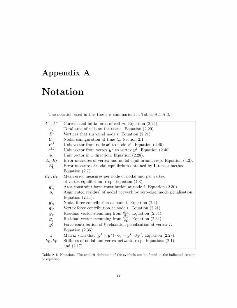
Appendix A
Notation
The notation used in this thesis is summarised in Tables A.1-A.3.
Am, Am0 Current and initial area of cell m. Equation (2.24).AT Total area of cells on the tissue. Equation (2.29).Bi Vertices that surround node i. Equation (2.21).Cn Nodal configuration at time tn. Section 2.1.eij Unit vector from node xj to node xi. Equation (2.40)eIJ Unit vector from vertex yJ to vertex yI . Equation (2.40)ez Unit vector in z direction. Equation (2.28).
Ei, EI Error measures of vertex and nodal equilibrium, resp. Equation (4.2).EiL Error measure of nodal equilibrium obtained by L-tensor method.
Equation (2.7).ED, EV Mean error measures per node of nodal and per vertex
of vertex equilibrium, resp. Equation (4.3).giA Area constraint force contribution at node i. Equation (2.30).gc Augmented residual of nodal network by zero-eigenmode penalisation.
Equation (2.11).giD Nodal force contribution at node i. Equation (2.2).giV Vertex force contribution at node i. Equation (2.21).
gx Residual vector stemming from ∂W∂x . Equation (2.34).
gy Residual vector stemming from ∂W∂ξ . Equation (2.34).
gIξ Force contribution of ξ-relaxation penalisation at vertex I.
Equation (2.35).J Matrix such that (yI × yJ) · ez = yI · JyJ . Equation (2.28).
kD, kV Stiffness of nodal and vertex network, resp. Equations (2.1)and (2.17).
Table A.1: Notation. The explicit definition of the symbols can be found in the indicated sectionor equation.
77
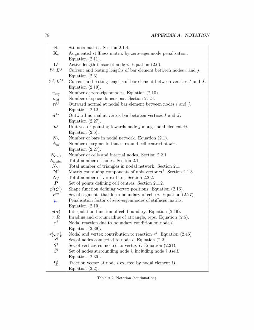
78 APPENDIX A. NOTATION
K Stiffness matrix. Section 2.1.4.Kc Augmented stiffness matrix by zero-eigenmode penalisation.
Equation (2.11).Li Active length tensor of node i. Equation (2.6).
lij , Lij Current and resting lengths of bar element between nodes i and j.Equation (2.3).
lIJ , LIJ Current and resting lengths of bar element between vertices I and J .Equation (2.19).
neig Number of zero-eigenmodes. Equation (2.10).nsd Number of space dimensions. Section 2.1.3.nij Outward normal at nodal bar element between nodes i and j.
Equation (2.12).nIJ Outward normal at vertex bar between vertices I and J .
Equation (2.27).nj Unit vector pointing towards node j along nodal element ij.
Equation (2.6).ND Number of bars in nodal network. Equation (2.1).Nm Number of segments that surround cell centred at xm.
Equation (2.27).Ncells Number of cells and internal nodes. Section 2.2.1.Nnodes Total number of nodes. Section 2.1.Ntri Total number of triangles in nodal network. Section 2.1.Nj Matrix containing components of unit vector nj . Section 2.1.3.NV Total number of vertex bars. Section 2.2.2.P Set of points defining cell centres. Section 2.1.2.
pi(ξI) Shape function defining vertex positions. Equation (2.16).Pm Set of segments that form boundary of cell m. Equation (2.27).pr Penalisation factor of zero-eigenmodes of stiffness matirx.
Equation (2.10).q(α) Interpolation function of cell boundary. Equation (2.16).r,R Inradius and circumradius of atriangle, reps. Equation (2.5).ri Nodal reaction due to boundary condition on node i.
Equation (2.39).riD, r
iV Nodal and vertex contribution to reaction ri. Equation (2.45)
Si Set of nodes connected to node i. Equation (2.2).SI Set of vertices connected to vertex I. Equation (2.21).Si Set of nodes surrounding node i, including node i itself.
Equation (2.30).
tijD Traction vector at node i exerted by nodal element ij.Equation (2.2).
Table A.2: Notation (continuation).

79
tIJV Traction vector at vertex I exerted by vertex element IJ .Equation (2.19).
tn nth time-step. Section 2.1.T I Triangle where vertex I is located. Section 2.1.T n Connectivity of nodal network at time tn. Section 2.1.tolR Aspect ratio tolerance. Equation (2.5).u Displacement vector. Equation (2.10).WA Energy term associated to area penalisation. Equation (2.24).Wc Augmented energy of nodal network by penalisation of
zero-eigenmodes. Equation (2.10).
WD,WijD Total nodal strain energy and strain energy of nodal element ij.
Equation (2.1).WV ,W
IJV Total vertex strain energy and strain energy of
vertex element IJ . Equation (2.17).xi Position of node i. Section 2.1.Xn List of nodal positions at time tn. Section 2.1.yI Position of vertex I. Section 2.2.1.α Local coordinate of points in vertex bars. Equation (2.16).γ Remodelling rate in rheological model. Equation (3.9).δ Numerical precision. Section 2.1.4.δIJ Kronecker delta. Equation (2.38).
δpqmj , δPQIJ See definitions in equation (2.43).
∆t Time increment. Equation (3.8).ε Distance of each off-set node from the corresponding boundary node.
Equation (2.12).εc Contractility of bar elements. Equation (3.15).
εcD, εcV Contractility employed in nodal and vertex network. Section 4.5.
εij , εIJ Strain at nodal and vertex bar elements, resp.Equations (2.1) and (2.17).
η Viscousity. Equation (3.3).θij , θIJ Inverse of resting lengths Lij and LIJ , resp. Section 2.2.5.κ Eigen value of system stiffness matrix K. Section 2.1.4.λA Penalty terms for area constraint. See equation (2.24).λL Penalisation factor of regularisation term. Equation (2.44).λξ Penalty terms for ξ-relaxation. See equation (2.31).
ξI Local coordinate of vertex I in triangle T I . Section 2.2.1.πD, πV Nodal and vertex contributions in EPM, resp. Equation (2.45).πF , πS Functionals of full- and split-network EPM.
Equations (2.39) and (2.45).σ Stress. Equation (3.1).Ωi Domain of cell i. Section 2.2.1.
Table A.3: Notation (continuation).


Appendix B
Inradius and circumradius
B.1 Inradius
In 2-D Euclidean geometry, inradius, r, of a triangle is the radius of the circletangetial to the sides of the triangle. Incentre is the centre of this circle.
Ir
C
B
A
rr
c
ba
Figure B.1: 4ABC and its incircle
Let I be the incentre of 4ABC.
Let r be the inradius of 4ABC.
The total area of 4ABC, A, is equal to the sum of the areas of the trianglesformed by the vertices of 4ABC and its incentre:
A = A4AIB +A4BIC +A4CIA. (B.1)
Let AB, BC and CA be the bases of 4AIB, 4BIC and 4CIA respectively.
81

82 APPENDIX B. INRADIUS AND CIRCUMRADIUS
The length of AB, BC and CA respectively are c, a and b.
The altitude of each of these triangles is r. Thus from are of triangle in termsof side and altitude:
A4AIB =cr
2
A4BIC =ar
2
A4CIA =br
2.
(B.2)
Thus, from (B.1) and (B.2) we have,
r =2A
a+ b+ c. (B.3)
B.2 Circumradius
The circumradius, R, of a triangle is the radius of the circle in which the trianglecan be inscribed. Circumcentre is the centre of this circle.
h
O
c
b a
E
D
C
BA
R
Figure B.2: 4ABC and its circumcircle
Let O be the circumcentre of 4ABC.
Let A be the area of 4ABC.
Let a perpendicular be dropped from C to AB at E.
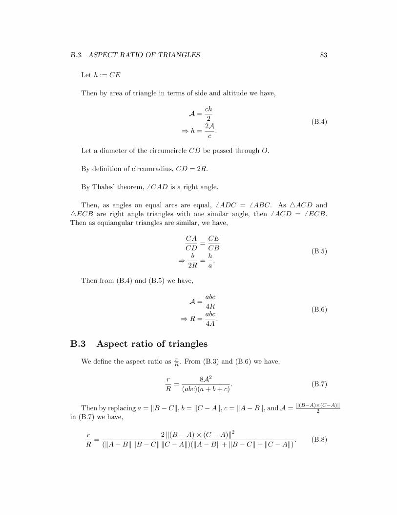
B.3. ASPECT RATIO OF TRIANGLES 83
Let h := CE
Then by area of triangle in terms of side and altitude we have,
A =ch
2
⇒ h =2Ac.
(B.4)
Let a diameter of the circumcircle CD be passed through O.
By definition of circumradius, CD = 2R.
By Thales’ theorem, 6 CAD is a right angle.
Then, as angles on equal arcs are equal, 6 ADC = 6 ABC. As 4ACD and4ECB are right angle triangles with one similar angle, then 6 ACD = 6 ECB.Then as equiangular triangles are similar, we have,
CA
CD=CE
CB
⇒ b
2R=h
a.
(B.5)
Then from (B.4) and (B.5) we have,
A =abc
4R
⇒ R =abc
4A.
(B.6)
B.3 Aspect ratio of triangles
We define the aspect ratio as rR . From (B.3) and (B.6) we have,
r
R=
8A2
(abc)(a+ b+ c). (B.7)
Then by replacing a = ‖B − C‖, b = ‖C −A‖, c = ‖A−B‖, andA = ‖(B−A)×(C−A)‖2
in (B.7) we have,
r
R=
2 ‖(B −A)× (C −A)‖2(‖A−B‖ ‖B − C‖ ‖C −A‖)(‖A−B‖+ ‖B − C‖+ ‖C −A‖) . (B.8)

84 APPENDIX B. INRADIUS AND CIRCUMRADIUS
B.4 Aspect ratio of tetrahedrons
In three-dimensional Euclidean Geometry, a tetrahedron inradius, r, is the radiusof the sphere tangetial to the faces of the tetrahedron, whereas circumradius of atetrahedron is defined as the radius of the sphere circumscribed to it. Given A, B,C, and D the coordinates of the tetrahedron vertices are
A = (Ax, Ay, Az),
B = (Bx, By, Bz),
C = (Cx, Cy, Cz),
D = (Dx, Dy, Dz).
Then by resorting to the following parentheses (Casey, 1988)
α =
∣∣∣∣∣∣∣∣
Ax Ay Az 1Bx By Bz 1Cx Cy Cz 1Dx Dy Dz 1
∣∣∣∣∣∣∣∣,
NABC = (B −A)× (C −A),
γ =
∣∣∣∣∣∣∣∣
A2x +A2
y +A2z Ax Ay Az
B2x +B2
y +B2z Bx By Bz
C2x + C2
y + C2z Cx Cy Cz
D2x +D2
y +D2z Dx Dy Dz
∣∣∣∣∣∣∣∣,
Fx =
∣∣∣∣∣∣∣∣
A2x +A2
y +A2z Ay Az 1
B2x +B2
y +B2z By Bz 1
C2x + C2
y + C2z Cy Cz 1
D2x +D2
y +D2z Dy Dz 1
∣∣∣∣∣∣∣∣, Fy =
∣∣∣∣∣∣∣∣
A2x +A2
y +A2z Ax Az 1
B2x +B2
y +B2z Bx Bz 1
C2x + C2
y + C2z Cx Cz 1
D2x +D2
y +D2z Dx Dz 1
∣∣∣∣∣∣∣∣,
Fz =
∣∣∣∣∣∣∣∣
A2x +A2
y +A2z Ax Ay 1
B2x +B2
y +B2z Bx By 1
C2x + C2
y + C2z Cx Cy 1
D2x +D2
y +D2z Dx Dy 1
∣∣∣∣∣∣∣∣,
the inraduis, r, of the tetrahedron can be computed as
r =|α|
‖NABC‖+ ‖NABD‖+ ‖NACD‖+ ‖NBCD‖, (B.9)
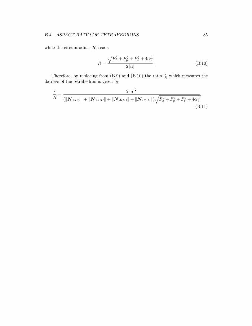
B.4. ASPECT RATIO OF TETRAHEDRONS 85
while the circumradius, R, reads
R =
√F 2x + F 2
y + F 2z + 4αγ
2 |α| . (B.10)
Therefore, by replacing from (B.9) and (B.10) the ratio rR which measures the
flatness of the tetrahedron is given by
r
R=
2 |α|2
(‖NABC‖+ ‖NABD‖+ ‖NACD‖+ ‖NBCD‖)√F 2x + F 2
y + F 2z + 4αγ
.
(B.11)


Appendix C
Proof of uniqueness of activelength tensor Li
We will here prove that the solution of the system of equations in (2.8) at a givennode i is unique if the vectors nj that define the cell–cell connectivities at node iand that form matrix A span Rnsd .
By definition, matrix A is semi-positive definite (SPD) and symmetric. We willhere prove that matrix A is in fact positive definite (PD) when the vectors nj spanRnsd , and hence gives a unique solution. Matrix A is PD if the following implicationholds:
LiTALi = 0⇒ Li = 0. (C.1)
But, by setting lij = Linj , we have that,
LiTALi =Si∑
j=1
Linj · Linj =Si∑
j=1
∥∥lij∥∥2.
So,
Si∑
j=1
Linj · Linj = 0⇒ lij = 0, ∀j, (C.2)
i.e., implication in (C.1) may be also expressed as,
Si∑
j=1
Linj · Linj = 0⇒ Linj · ek = 0, ∀j, k.
87

88APPENDIX C. PROOF OF UNIQUENESS OF ACTIVE LENGTH TENSOR LI
Setting nj = αjl el we have that,
Linj · ek = αjlLiel · ek =
∑
l
αjlLikl,
with Likl = Liel · ek the component kl of tensor Li. Therefore, (C.2) is equivalentto,
∑
l
αjlLikl = 0, ∀k, j.
By denoting by Lik the k-th row of the tensor Li, this condition may be alsoexpressed as,
nj · Lik = 0, ∀k, j,
that is, the vector nj are orthogonal to each one of the rows of Li. If the vectorsnj span the whole space Rnsd , this is only possible when Lik = 0, as we wanted toprove. If the tensor Li is not assumed symmetric, the uniqueness of the solution canbe also proved by considering an alternative matrix Nj in the definition of matrixA, but following very similar steps.

Appendix D
Voronoi diagram
Consider 4ABC with vertices at XA, XB, XC and the intersection of theperpendicular bisectors P at XP . Bisectors of 4ABC intersect with the sides ofthe triangle at L, M and N . XP can be interpolated in terms of XA, XB and XC
A
BC
NM
L
P
Figure D.1: 4ABC and its perpendicular bisectors
so that,
XP = αXA + βXB + γXC ,
where based on barycentric coordinates,
α =S4PBCS4ABC
, β =S4APCS4ABC
, γ =S4ABPS4ABC
. (D.1)
89
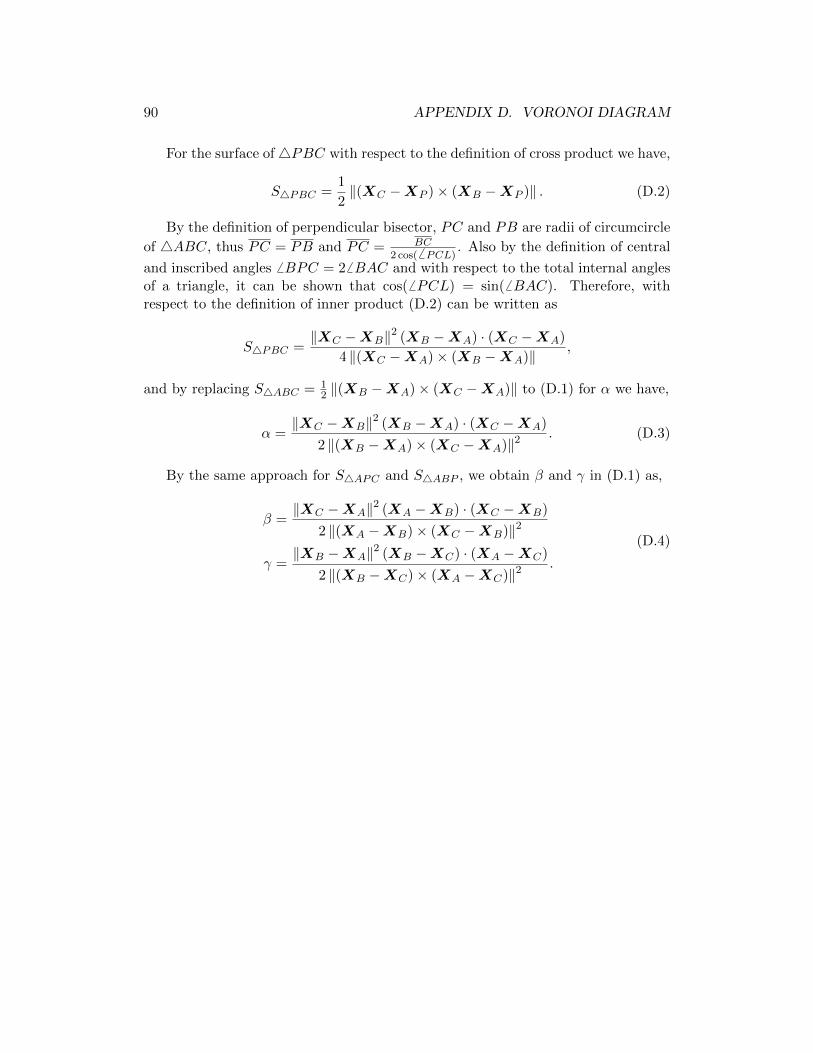
90 APPENDIX D. VORONOI DIAGRAM
For the surface of4PBC with respect to the definition of cross product we have,
S4PBC =1
2‖(XC −XP )× (XB −XP )‖ . (D.2)
By the definition of perpendicular bisector, PC and PB are radii of circumcircle
of 4ABC, thus PC = PB and PC = BC2 cos( 6 PCL)
. Also by the definition of central
and inscribed angles 6 BPC = 26 BAC and with respect to the total internal anglesof a triangle, it can be shown that cos( 6 PCL) = sin( 6 BAC). Therefore, withrespect to the definition of inner product (D.2) can be written as
S4PBC =‖XC −XB‖2 (XB −XA) · (XC −XA)
4 ‖(XC −XA)× (XB −XA)‖ ,
and by replacing S4ABC = 12 ‖(XB −XA)× (XC −XA)‖ to (D.1) for α we have,
α =‖XC −XB‖2 (XB −XA) · (XC −XA)
2 ‖(XB −XA)× (XC −XA)‖2. (D.3)
By the same approach for S4APC and S4ABP , we obtain β and γ in (D.1) as,
β =‖XC −XA‖2 (XA −XB) · (XC −XB)
2 ‖(XA −XB)× (XC −XB)‖2
γ =‖XB −XA‖2 (XB −XC) · (XA −XC)
2 ‖(XB −XC)× (XA −XC)‖2.
(D.4)
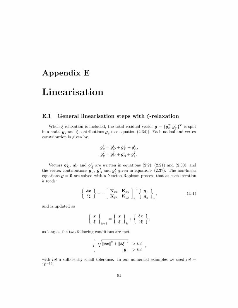
Appendix E
Linearisation
E.1 General linearisation steps with ξ-relaxation
When ξ-relaxation is included, the total residual vector g = gTx gTy T is splitin a nodal gx and ξ contributions gy (see equation (2.34)). Each nodoal and vertexconstribution is given by,
gix = giD + giV + giA,
gIy = gIV + giA + gIξ .
Vectors giD, giV and giA are written in equations (2.2), (2.21) and (2.30), andthe vertex contributions gIV , gIA and gIξ given in equations (2.37). The non-linearequations g = 0 are solved with a Newton-Raphson process that at each iterationk reads:
δxδξ
= −
[Kxx Kxy
Kyx Kyy
]−1
k
gxgy
k
, (E.1)
and is updated as
xξ
k+1
=
xξ
k
+
δxδξ
,
as long as the two following conditions are met,
√‖δx‖2 + ‖δξ‖2 > tol
‖g‖ > tol,
with tol a sufficiently small tolerance. In our numerical examples we used tol =10−10.
91

92 APPENDIX E. LINEARISATION
The block matrices in (E.1) correspond to the following linearisation terms,
Kijxx =
∂giD∂xj
+∂giV∂xj
+∂giA∂xj
(E.2)
KiJxy =
∂giV∂ξJ
+∂giA∂ξJ
(E.3)
KIjyx =
∂gIV∂xj
+∂gIA∂xj
KIJyy =
∂gIV∂ξJ
+∂gIA∂ξJ
+∂gIξ
∂ξJ, (E.4)
where due to the expressions of giD and gIξ , we have used the fact that∂giD∂yJ
and∂gIξ∂xj
vanish. Also note that since our equlibrium equations stem from the linearisationof an energy function W (x, ξ), we have that,
KiJxy =
∂2(WV +WA)
∂xi∂ξJ=
[∂2(WV +WA)
∂ξI∂xj
]T= KIj
yxT.
In the next sections we will give the linearisation of the terms in (E.2)-(E.4).
E.2 Linearisation of nodal and vertex tractions tijD andtIJV
Many of the derivations detailed below will involve the linearisation of the trac-tion vectors given in equations (3.14),
tijD =∂W ij
D
∂xi=εij
Lij
(1− lij
Lij∂Lij
∂lij
)eij
tIJV =∂W IJ
V
∂yI=εIJ
LIJ
(1− lIJ
LIJ∂LIJ
∂lIJ
)eIJ .
The factor ∂L∂l is zero when the resting length is constant, but for the rheological
law presented in Chapter 3 , this factor is given in equations (3.11) and (3.17). Inthe subsequent expressions we will need the derivatives of the traction vectors above.We define matrix
Kiit :=
∂tijD∂xi
= −∂tjiD
∂xi= −Kji
t = −Kijt = Kjj
t , (E.5a)
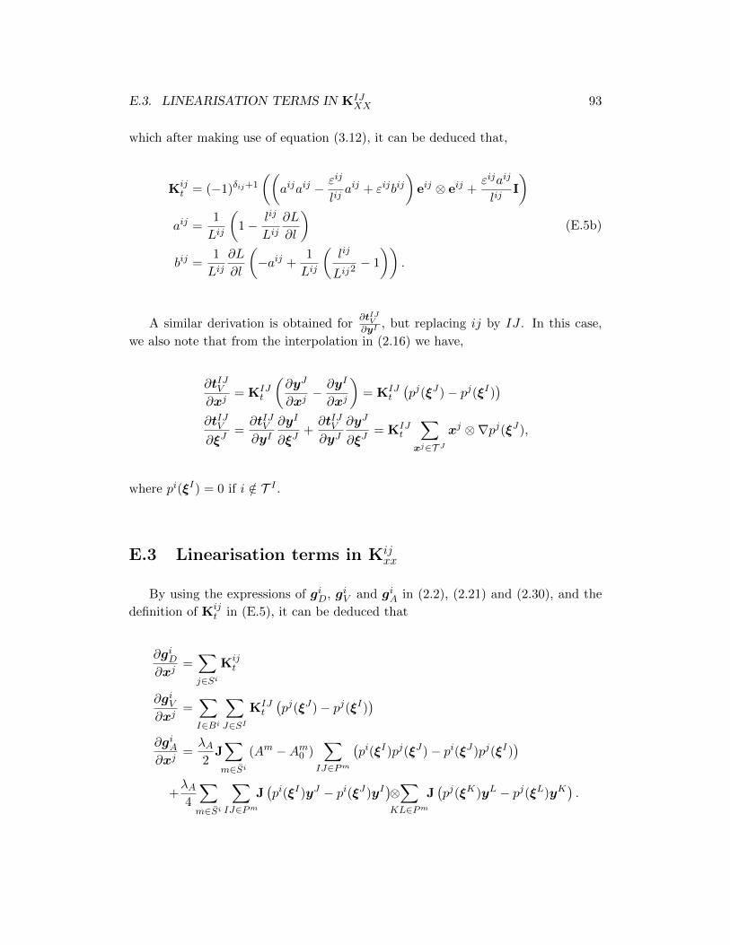
E.3. LINEARISATION TERMS IN KIJXX 93
which after making use of equation (3.12), it can be deduced that,
Kijt = (−1)δij+1
((aijaij − εij
lijaij + εijbij
)eij ⊗ eij +
εijaij
lijI
)
aij =1
Lij
(1− lij
Lij∂L
∂l
)
bij =1
Lij∂L
∂l
(−aij +
1
Lij
(lij
Lij2 − 1
)).
(E.5b)
A similar derivation is obtained for∂tIJV∂yI
, but replacing ij by IJ . In this case,
we also note that from the interpolation in (2.16) we have,
∂tIJV∂xj
= KIJt
(∂yJ
∂xj− ∂yI
∂xj
)= KIJ
t
(pj(ξJ)− pj(ξI)
)
∂tIJV∂ξJ
=∂tIJV∂yI
∂yI
∂ξJ+∂tIJV∂yJ
∂yJ
∂ξJ= KIJ
t
∑
xj∈T Jxj ⊗∇pj(ξJ),
where pi(ξI) = 0 if i /∈ T I .
E.3 Linearisation terms in Kijxx
By using the expressions of giD, giV and giA in (2.2), (2.21) and (2.30), and the
definition of Kijt in (E.5), it can be deduced that
∂giD∂xj
=∑
j∈SiKijt
∂giV∂xj
=∑
I∈Bi
∑
J∈SIKIJt
(pj(ξJ)− pj(ξI)
)
∂giA∂xj
=λA2
J∑
m∈Si(Am −Am0 )
∑
IJ∈Pm
(pi(ξI)pj(ξJ)− pi(ξJ)pj(ξI)
)
+λA4
∑
m∈Si
∑
IJ∈PmJ(pi(ξI)yJ − pi(ξJ)yI
)⊗∑
KL∈PmJ(pj(ξK)yL − pj(ξL)yK
).

94 APPENDIX E. LINEARISATION
E.4 Linearisation terms in KiJxy
From the expressions of giV and giA in (2.21) and (2.30), and from equation(2.36), it can be also deduced that,
∂giV∂ξJ
=
∑
K∈SJtJKV
⊗∇pi(ξJ) +
∑
I∈Bipi(ξI)
∑
J∈SIKIJt
∂yJ
∂ξJ
∂giA∂ξJ
=λA2
J∑
m∈Si(Am −Am0 )
Nm∑
IJ∈Pm
(pi(ξI)
∂yJ
∂ξJ− yI ⊗∇pi(ξJ)
)
+λA2
J∑
m∈Si
Nm∑
IJ∈Pm
(pi(ξI)yJ − pi(ξJ)yI
)⊗ ∂Am
∂ξJ,
with ∂Am
∂ξJgiven in (2.38).
E.5 Linearisation terms in KIJyy
The linearisation of gIV , gIA and gIξ in (2.37) yields,
∂gIV∂ξJ
=∑
K∈SI
∑
i∈T I
(∇pi(ξI)⊗ xi
)(KIIt δIJ
∂yI
∂ξJ+ KIK
t δKJ∂yK
∂ξJ
)
∂gIA∂ξJ
= λA
Nnodes∑
m=1
∂Am
∂ξI⊗ ∂Am
∂ξJ+ λA
Nnodes∑
m=1
(Am −Am0 )∂2Am
∂ξI∂ξJ
∂gIξ
∂ξJ= λξδIJI,
where the expressions of ∂yI
∂ξIand ∂Am
∂ξIare given in (2.36) and in (2.38), respectively,
and
∂2Am
∂ξI∂ξJ=
∑
KL∈Pm
(δKIδLJ
(∂yK
∂ξI
)TJ∂yL
∂ξJ− δLIδKJ
(∂yL
∂ξI
)TJ∂yK
∂ξJ
).
Bibliography
Alt S, Ganguly P, and Salbreux G. Vertex models: from cell mechanics to tissuemorphogenesis. Philos. Trans. R. Soc. London B. Biol. Sci., 372(1720), 2017.http://dx.doi.org/10.1098/rstb.2015.0520.
Antunes M, Pereira T, Cordeiro JV, Almeida L, and Jacinto A. Coordinated wavesof actomyosin flow and apical cell constriction immediately after wounding. J.Cell Biol., 202(2):365–379, 2013.
Arroyo M and DeSimone A. Shape control of active surfaces inspired by the move-ment of euglenids. J. Mech. Phys. Solids, 62:99–12, 2014.
Asadipour N, Trepat X, and Munoz JJ. Porous-based rheological model for tissuefluidisation. J. Mech. Phys. Solids, 96:535–549, 2016.
Babuska I and Aziz A. On the angle condition in the finite element method. SIAMJ. Numer. Analysis, 13:214–227, 1976.
Barber C, Dobkin D, and Huhdanpaa HT. The quickhull algorithm for convex hulls.ACM Trans. Math. Softw., 22(4):469–483, 1996. http://www.qhull.org
Beret C, Sulak L, and Lecuit T. Myosin-dependent junction remodelling controlsplanar cell intercalation and axis elongation. Lett. Nat., 429:667–671, 2004.
Bergdorf M, Milde F, and Koumoutsakos P. Multiscale Cancer Modeling, Chapter11, pages 213–237. Chapman and Hall/CRC mathematical and ComputationalBiology, 2010.
Besser A, Colombelli J, Stelzer EHK, and Schwarz US. Viscoelastic response ofcontractile filament bundles. Phys. Rev. E, 83(051902), 2011.
Bi D, Yang X, Marchetti MC, and Manning ML. Motility-Driven Glass and JammingTransitions in Biological Tissues. Phys. Rev. X., 6:021011, 2016.
Bittig T, Wartlick O, Kicheva A, Gonzalez-Gaitan M, and Julicher F. Dynamics ofanisotropic tissue growth. New J. Phys., 10(063001), 2008.
95

96 BIBLIOGRAPHY
Brodland GW. Computational modeling of cell sorting, tissue engulfment, andrelated phenomena: a review. Appl. Mech. Rev., 57:1–30, 2004.
Brugues A, Anon E, Conte V, Veldhuis J, Gupta M, Collombelli J, Monuz JJ,Brodland GW, Landoux B, and Trepat X. Forces driving epithelial wound healing.Nature Phys., 10:683–690, 2014.
Carreira-Perpinan MA. A review of dimension reduction techniques. Tech. Rep.,CS-96-09, Department of Computer Science, University of Shefflield, UK, 1997.
Casey J. A Sequel to the First Six Books of the Elements of Euclid, Containing anEasy Introduction to Modern Geometry with Numerous Examples. Hodges, Figgis& Co., Dublin, 5th edition, 1988.
Chaudhuri O, Parekh S, and Fletcher D. Reversible stress softening of actin net-works. Nature, 445:295–298, 2007.
Clement R, Collinet C, Dehapiot B, Lecuit T, and Lenne PF. Viscoelastic dissi-pation stabilizes cell shape changes during tissue morphogenesis. BioRxiv., 2017.doi.org/10.1101/107557
Costa M, Sweeton D, and Wieschaus E. The development of Drosophilamelanogaster. Chapter 8: Gastrulation in Drosophila: cellular mechanisms ofmorphogenetic movements. Cold Spring Laboratory Press, New York, 1993.
Cueto E, Calvo B, and Doblare M. Modelling three-dimensional piece-wise homo-geneous domains using the α-shape-based natural element method. Int. J. Num.Meth. Engng., 54(6):871–897,2002. doi:10.1002/nme.452.
Davidson LA, Joshi SD, Kim HY, von Dassow M, Zhang L, and Zhou J. Emergentmorphogenesis: Elastic mechanics of a self-deforming tissue. J. Biomech., 43:63–70, 2010.
Doubrovinski K, Swan M, Polyakov O, and Wieschaus E. Measurement of corticalelasticity in Drosophila melanogaster embryos using ferrofluids. Proc. Nat. Acad.Sci. USA, 114 (5):1051–1056, 2017.
Edelsbrunner H and Mucke EP. Three-dimensional alpha shapes. ACM Trans.Graph., 13(1):43–72, 1994.
Fernandez-Sanchez M, Barbier S, Whitehead J, Bealle G, Michel A, Latorre-OssaH, Rey C, Fouassier L, Claperon A, Brulle L, Girard E, Servant N, Rio-Frio T,Marie H, Lesieur S, Housset C, Gennisson J, Tanter M, Menager C, Fre S, RobineS, and Farge E. Mechanical induction of the tumorigenic β-catenin pathway bytumour growth pressure. Nature, 523(7558):92–95, 2015.

BIBLIOGRAPHY 97
Findley WN, Lai JS, and Onaran K. Creep and Relaxation of Nonlinear ViscoelasticMaterials: With an Introduction to Linear Viscoelasticity. Dover,New York, 1989.
Fletcher AG, Mirams GR, Murray PJ, Walter A, Kang JW, Cho KH, Maini PK,and Byrne HM. Multiscale Cancer Modeling, Chapter 6, pages 111–134. Chapmanand Hall/CRC Mathematical and Computational Biology, 2010.
Fletcher AG, Osborne J, Maini P, and Gavaghan D. Implementing ver-tex dynamics models of cell polulations in biology within a consistentcomputational framework. Prog. Byoph. Mol. Biol., 113(2):299–326, 2013.doi:http://dx.doi.org/10.1016/j.pbiomolbio.2013.09.003.
Forgacs G, Foty RA, Shafrir Y, and Steinberg MS. Viscoelastic properties of livingembryonic tissues: a quantitative study. Bioph. J., 74(2227), 1998.
Frieboes H, Lowengrub J, Wise S, Zheng X, Macklin P, Bearer E, and Cristini V.Computer simulation of glioma growth and morphology. Neuroimage, 37:59–70,2007.
Fu L, Hu XY, and Adams NA. A physics-motivated centroidal Voronoi particledomain decomposition method. J. Comp. Phys., 335:718–735 , 2017.
Fung YC. Biomechanics: Mechanical Properties of Living Tissues. Springer, NewYork, 2nd edition, 1993.
Galle J, Loeffler M, and Drasdo D. Modeling the effect of deregulated proliferationand apoptosis on the growth dynamics of epithelial cell populations in vitro.Bioph. J., 88:62–75, 2005.
Gatsonis A and Spirkin A. A three-dimensional electrostatic particle-in cell method-ology on unstructured Delaunay-Voronoi grids. J. Comp. Phys., 228(10):3742–3761, 2009.
Ghosh S and Moorthy S. Three-dimensional Voronoi cell finite element model formicrostructures with ellipsoidal heterogeneities. Comput. Mech., 10(34):510–531,2004.
Gittes F and MacKintosh FC. Dynamic shear modulus of a semiflexible polymernetwork. Phys. Rev. E, 58(R1241),1998.
Gonzalez D, Cueto E, Chinesta F, and Doblare M. A natural element updatedlagrangian strategy for free-surface fluid dynamics. J. Comp. Phys., 223(1):127–150, 2007.
Gonzalez-Valverde I and Garcıa-Aznar JM. A hybrid computational model to ex-plore the topological characteristics of epithelial tissues. Int. J. Num. Meth.Biomed. Engng., 2017. doi: 10.1002/cnm.2877.

98 BIBLIOGRAPHY
Gregor T, Bialek W, de Ruyter van Stevininck RR, Tank DW, and Wieschaus EF.Diffusion and scaling during early embryonic pattern formation. Proc. Nat. Acad.Sci. USA, 102(18403), 2005.
Guittet A, Lepilliez M, Tanguy S, and Gibou F. Solving elliptic problems withdiscontinuities on irregular domains - the Voronoi Interface Method. J. Comp.Phys., 298:747–765, 2015.
Hardin J and Keller R. The behaviour and function of bottle cells during gastrulationof Xenopus laevis. Development, 103: 211–230, 1988.
Hardin J and Walston T. Models of morphogenesis: the mechanisms and mechanicsof cell rearrangement. Curr. Opin. Genet. & Dev., 14 (4):399–406, 2004.
Harris AR, Bellis J, Khalilgharibi N, Wyatt T, Baum B, Kabla AJ, and CharrasGT. Generating suspended cell monolayers for mechanobiological studies. Nat.Protoc., 8 (12):2516–2530, 2013.
Harris AR, Peter L, Bellis J, Baum B, Kabla AJ, and Charras GT. Characterizingthe mechnics of cultured cell monolayers. Proc. Nat. Acad. Sci. USA, 109 (41):16,449–16, 454, 2012.
Holpzafel GA. Nonlinear Solid Mechanics: A continuum Approach for Engineering.John Wiley and & Sons, Chichester, 5th edition, 2007.
Honda H, Motosugi N, Nagai T, Tanemura M, and Hiiragi T. Computer simulationof emerging asymmetry in the mouse blastocyte. Development, 135(8):1407–1414,2008.
Honda H, Ogita Y, Higuchi S, and Kani K. Cell movements in a living mammaliantissue: long-term observation of individual cells in wounded corneal endothelia ofcats. J. Morphol., 174, 25–39, 1982.
Honda H, Tanemura M, and Nagai T. Geometrical models for cells in tissues. Int.Rev. Cytol., 1983(81):191–248, 1983.
Honda H, Tanemura M, and Nagai T. A three-dimensional vertex dynamics cellmodel of space-filling polyhedra simulating cell behaviour in a cell aggregate. J.Theor. Biol., 226:439–453, 2004.
Jacobs CR, Huang H, and Kwon RY. Introduction to cell mechanics and mechanobi-ology, chapter 1, pages 1–15. Garland Science, 1st edition, 2012.
Janmey PS, Hivdt S, Kas J, Lerche D, Maggs A, Sackmann E, Schliwa M, andStossel TP. Softness, strength and self-repair in intermediate filament networks.J. Biol. Chem., 269(32503), 1994.

BIBLIOGRAPHY 99
Keller R, Davidson LA, and Shook DR. How we are shaped: The biomechanics ofgastrulation. Differentiation, 71: 171–205, 2003.
Khalilgharibi N, Fouchard J, Asadipour N, Yonis A, Harris A, Mosaffa P, FujitaY, Kabla A, Baum B, Munoz JJ and Charras GT. Stress relaxation in epithe-lial monolayers arises from length change controlled by actomyosin. Manuscriptsubmitted for publication.
Krul T, Kaandorp J, and Blom JG. Modeling developmental regulatory networks.Lect. Notes. Comput. Sc., 2660:688–697, 2003.
Lambert T. The Delaunay triangulation maximizes the mean inradius. Proceedingsof the 6th Canadian Conference on Computational Geometry (CCCG94), 201–206, 1994.
Lecuit T and Lenne PF. Cell surface mechanics and the control of cell shape, tissuepatterns and morphogenesis. Nat. Rev., 8:633–644, 2007.
Lee JA and Verleysen M. Nonlinear Dimensionality Reduction. Information scienceand statistics, Springer, New York, 2007.
Leptin M and Grunewald B. Cell shape changes during gastrulation in Drosophila.Development, 110:72–84, 1990.
Lewis H. Mechanics of invagination. Anat. Rec., 97: 139–156, 1947.
Lin IE and Taber LA. Mechanical effects of looping in the embryonic chick heartmorphogenesis. J. Biomech., 27:311–321, 1994.
Ma X, Lynch HE, Skully PC, and Hutson MS. Probing embryonic tissue mechanicswith laser hole drilling. Phys. Biol., 6(3):036004, 2009.
der Maaten LJPV, Postma EO, and den Herik HJV. Dimensionality Reduction: Acomprehensive review. TiCC TR, 2009–5, Tilburg University, The Netherlands,2009.
MacKintosh FC, Kas J, and Janmey PA. Elasticity of semiflexible biopolymer net-works. Phys. Rev. Letters, 75(4425), 1995.
MacKintosh FC and Levine AJ. Nonequilibrium mechanics and dynamics of motor-activated gels. Phys. Rev. Letters, 100(018104), 2008.
Macklin P, Edgerton ME, Lowengrub JS, and Cristini V. Multiscale Modelling ofCancer, Chapter 6, pages 88–122. Cambridge University Press, Cambridge, UK,2010.
Macklin P and Lowengrub JS. Nonlinear simulation of the effect of microenviron-ment on tumor growth. J. Theor. Biol., 245:677–704, 2007.

100 BIBLIOGRAPHY
Millan D, Rosolen A, and Arroyo M. Non-linear manifold learning for mesh-freefinite deformations thin shell analysis. Int. J. Num. Methods Eng., 93 (7): 685–713, 2013.
Mizuno D, Tardin C, Schmidt CF, and MacKintosh FC. Nonequilibrium mechanicsof active cytoskeletal networks. Science, 315(5810):370–373, 2007.
Moeendarbary E, Valon L, Fritzsche M, Harris A, Moulding D, Thrasher A, StrideE, Mahadevan L, and Charras GT. The Cytoplasm of living cells behaves as aporoelastic material. Numer. Math., 12:253–261, 2013.
Moorthy S and Ghosh S. A model for analysis of arbitrary composite and porousmicrostructures with Voronoi cell finite elements. Int. J. Num. Meth. Engng.,39(14):2363–2398, 1996.
Morozof KI and Pismen LM. Motor-driven effective temperature and viscoelasticresponse of active matter. Phys. Rev. E, 81(061922),2010.
Mosaffa P, Asadipour N, Millan D, Rodrıguez-Ferran A, and Munoz JJ. Cell-centred model for the simulation of curved cellular monolayers. Comp. Part.Mech., 2(4):359–370, 2015.
Mosaffa P, Rodrıguez-Ferran A, and Munoz JJ. Hybrid cell-centred/vertex modelfor multicellular systems with equilibrium-preserving remodelling. Int. J. Num.Meth. Biomed. Engng., 2017 (in press).
Munjal A, Philippe J, Munro E, and Lecuit T. A self-organised biomechanical net-work drives shape changes during tissue morphogenesis. Nature, 524(7565):351–355, letter, 2015.
Munoz JJ and Albo S. Physiology-based model of cell viscoelasticity. Phys. Rev. E,88(012708), 2013.
Munoz JJ, Barrett K, and Miodownik M. A deformation gradient decompositionmethod for the analysis of the mechanics of morphogenesis. J. Biomech., 40:1372–1380, 2007.
Munoz JJ, Conte V, Asadipour N, and Miodownik M. A truss element for modellingreversible softening in living tissues. Mech. Res. Commun., 49:44–49, 2013.
Neumann JV and Burks AW. Theory of Self-Reproducing Automata. University ofIllinois Press, 1966.
Odell GM, Oster G, Alberch P, and Burnside B. The mechanical basis of morpho-genesis: I. Epithelial folding and invagination. Dev. Biology, 84:446–462, 1981.
Okabe A, Boots B, and Sugihara K. Spatial Tessellations: Concepts and Applicationsof Voronoi Diagrams. Wiley, New York, 1992.
BIBLIOGRAPHY 101
Okuda S, Inoue Y, Eiraku M, Adachi T, and Sasai Y. Vertex dynamics simulationsof viscosity-dependent deformation during tissue morphogenesis. Biomech. Model.Mechanobiol.,14(2):413–425, 2015.
Okuda S, Inoue Y, Eiraku M, Sasai Y, and Adachi T. Modeling cell proliferation forsimulating three-dimensional tissue morphogenesis based on a reversible networkreconnection framework. Biomech. Model. Mechanobiol., 12:987–996, 2013.
Osborne JM, Walter A, Kershaw SK, Mirams GR, Fletcher AG, PathmanathanP, Gavaghan D, Jensen OE, Maini PK, and Byrne HM. A hybrid approach tomultiscale modeling of cancer. Phil. Trans. Royal Soc. London A, 368:5013–5028,2010.
Pare AC, Vichas A, Fincher CT, Mirman Z, Farell DL, Mainieri A, and Zallen JA.A positional toll receptor code directs convergent extension in Drosophila Egg.Nature, 515:526–527, 2014.
Perrone M, Veldhuis J, and Brodland G. Dynamic analysis of spatial flexible multi-body systems using joint co-ordinates, Biomech. Model. Mechanobiol., 15(2):405–418, 2016.
Pitt-Francis J, Pathmanathan P, Bernabeu MO, Bordas R, Cooper J, Fletcher AG,Mirams GR, Murray P, Osborne JM, Walter A, Chapman SJ, Garny A, vanLeeuwen IMM, Maini PK, Rodrıguez B, Waters SL, Whiteley JP, Byrne HM,and Gavaghan DJ. Chaste: A test-driven approach to software development forbiological modelling. Comput. Phys. Commun., 180:2452–2471, 2009.
Ramis-Conde I, Drasdo D, Anderson ARA, and Chaplain MAJ. Modelling theinfluence of the E-cadherin-β-catenin pathway in cancer cell invasion: a multi-scale approach. Bioph. J., 95:155–165, 2008.
Razzell W, Wood W, and Martin P. Recapitulation of morphogenetic cell shapechanges enables wound re-epithelialisation. Development, 141(1814–1820), 2014.
Rejniak K. An immersed boundary framework for modelling the growth of individualcells: An application to early tumour development. J. Theor. Biol., 247(1):186–204, 2007.
Rodriguez EK, Hoger A, and McCulloch AD. Stress-dependent finite growth in softelastic tissues. J. Biomech., 27:455–467, 1994.
Roeland RMH and Glazier JA. A cell-centred approach to developmental biology.Physica A, 352:113–130, 2005.
Roweis ST and Saul LK. Think Globally, Fit Locally: Unsupervised learning oflow-dimensional manifolds. J. Mach. Learn. Res., 4:119–155, 2003.

102 BIBLIOGRAPHY
Roweis ST and Saul LK. Nonlinear dimensionality reduction by locally linear em-bedding. Science, 290: 2323–2326, 2000.
Salbreux G, Charras GT, and Paluch E. Actin cortex mechanics and cellular mor-phogenesis. Trends Cell Biol., 22 (10): 536–545, 2012.
Sandersius S and Newman T. Modelling cell rheology with the Subcellular ElementModel. Phys. Biol., 5(1)045008, 2008.
Sandersius S, Weijer C, and Newman T. Emergent cell and tissue dynamics forsubcellular modelling of active biomechanical processes. Phys. Biol., 8 (045007),2011.
Schaller G and Meyer-Hermann M. Multicellular tumor spheroid in an off-latticeVoronoi-Delaunay cell model. Phys. Rev. E, 71(51910), 2005.
Sibson R. A vector Identity for the Dirichlet tessellation. Math. Proc. Cambr. Phil.Soc., 87(1):151–155, 1980. doi:10.1017/S0305004100056589.
Slepchenko BM, Shaff JC, Macara I, and Loew LM. Quantitative cell biology withthe virtual cell model. Trends Cell Biol., 13:570–576, 2003.
Spahn P and Reuter R. Avertex model of Drosophila ventral furrow formation.PLOS ONE, 8(9):e75051, 2013.
Sukumar N. Voronoi cell finite difference method for the diffusion operator onarbitrary unstructured grids. Int. J. Num. Meth. Engng., 57(1):1–34, 2003.
Sunyer R, Conte V, Escribano J, Elosegui-Artola A, Labernadie A, Valon L, Nava-jas D, Garcıa-Aznar JM, Munoz JJ, Roca-Cusachs P, and Trepat X. Collectivecell durotaxis emerges from long-range intercellular force transmission. Science,353(6304):1157–1161, 2016. doi:10.1126/science.aaf7119.
Trepat X, Wasserman M, Angelini T, Millet E, Weitz D, Butler J, and Fredberg J.Physical forces during collective cell migration. Nat. Phys., 5(3):426–430, 2009.
Tomita M, Hashimoto K, Takahashi K, Shimizu T, Matsuzaki Y, Miyoshi F, SaitoK, Tanida S, Yugi K, Venter J, and Hatchison C. E-CELL: Software Environmentfor Whole-Cell Simulation. Bioinformatics, 15:72–84, 1999.
Walker DC, Southgate J, Hill G, Holcombe M, Hose DR, Wood SM, MacNail S, andSmallwood RH. The epitheliome: agent-based modelling of the social behaviourof cells. Biosystems, 76:89–100, 2004.
Wilson EL. A computer program for the dynamic stress analysis of undergroundstructures. UCB/SESM Report No. 68/01, University of California, Berkley, 1968.

BIBLIOGRAPHY 103
Zhang Z and Wang J. MLLE: Modified locally linear embedding using multipleweights. In: Scholkopf B, Platt J and Hoffman T (eds). Advances in NeuralInformation Processing Systems. 19, MIT Press, Cambridge, 1593–1600, 2007.