Statistical Computing

Hung Chen

hchen@math.ntu.edu.tw

Department of Mathematics

National Taiwan University

18th February 2004

Meet at NW 405 On Wednesday from 9:10 to 12.

1

Course Overview

•Monte Carlo methods for statistical inference

1. Pseudo-random deviate

2. Non-uniform variate generation

3. Variance reduction methods

4. Jackknife and Bootstrap

5. Gibbs sampling and MCMC

•Data partitioning and resampling (bootstrap)

1. Simulation Methodology

2. Sampling and Permutations (Bootstrap and per-mutation methods)

•Numerical methods in statistics

1. Numerical linear algebra and linear regressions2

2. Application to regression and nonparametric re-gression

3. Integration and approximations

4. Optimization and root finding

5. Multivariate analysis such as principal componentanalysis

• Graphical methods in computational statistics

• Exploring data density and structure

• Statistical models and data fitting

• Computing Environment: Statistical software R (“GNU’sS”)

– http://www.R-project.org/

– Input/Output

3

– Structured Programming

– Interface with other systems

• Prerequisite:

– Knowledge on regression analysis or multivariateanalysis

– Mathematical statistics/Probability theory; Statis-tics with formula derivation

– Knowledge about statistical software and experi-ence on programming languages such as Fortran,C and Pascal.

• Text Books:The course materials will be drawn from follow-ing recommended resources (some are available viaInternet) and others that will be made available

4

through the handout.

– Gentle, J.E. (2002) Elements of Computational Statis-tics. Springer.

– Hastie, T., Tibshirani, T. , Friedman, J.H. (2001)The Elements of Statistical Learning: Data Mining,Inference, and Prediction. Springer-Verlag.

– Lange, K. (1999) Numerical analysis for statisti-cians. Springer-Verlag, New York

– Ripley, B.D. and Venables, V.W. and BD (2002)Modern applied statistics with S, 4th edition. Springer-Verlag, New York.Refer to http://geostasto.eco.uniroma1.it/utenti/liseo/dispense R.pdf for a note of this book.

– Robert, C.P. and Casella, G. (1999). Monte Carlo

5

Statistical Methods. Springer Verlag.

– Stewart, G.W. (1996). Afternotes on NumericalAnalysis. SIAM, Philadelphia.

– An Introduction to R by William N. Venables, DavidM. Smith(http://www.ats.ucla.edu/stat/books/#DownloadableBooks)

• Grading: HW 50%, Project 50%

6

Outline

• Statistical Learning

– Handwritten Digit Recognition

– Prostate Cancer

– DNA Expression Microarrays

– Language

• IRIS Data

– Linear discriminant analysis

– R-programming

– Logistic regression

– Risk minimization

– Discriminant Analysis

•Optimization in Inference7

– Estimation by Maximum Likelihood

– Optimization in R

– EM Methods

∗ Algorithm

∗ Genetics Example(Dempster, Laird, and Rubin;1977)

– Normal Mixtures

– Issues

• EM Methods: Motivating example

– ABO blood groups

– EM algorithm

– Nonlinear Regression Models

– Robust Statistics

8

• Probability statements in Statistical Inference

• Computing Environment: Statistical software R (“GNU’sS”)

– http://www.R-project.org/

– Input/Output

– Structured Programming

– Interface with other systems

9

Introduction: Statistical Computing in Practice

Computationally intensive methods have become widelyused both for statistical inference and for exploratoryanalysis of data.The methods of computational statistics involve

• resampling, partitioning, and multiple transforma-tions of a data set

•make use of randomly generated artificial data

• function approximation

Implementation of these methods often requires ad-vanced techniques in numerical analysis, so there is aclose connection between computational statistics andstatistical computing.

10

In this course, we first address some areas of applica-tion of computationally intensive methods, such as

• density estimation

• identification of structure in data

•model building

• optimization

11

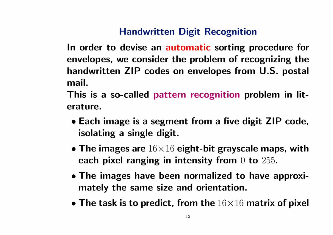
Handwritten Digit Recognition

In order to devise an automatic sorting procedure forenvelopes, we consider the problem of recognizing thehandwritten ZIP codes on envelopes from U.S. postalmail.This is a so-called pattern recognition problem in lit-erature.

• Each image is a segment from a five digit ZIP code,isolating a single digit.

• The images are 16×16 eight-bit grayscale maps, witheach pixel ranging in intensity from 0 to 255.

• The images have been normalized to have approxi-mately the same size and orientation.

• The task is to predict, from the 16×16 matrix of pixel12

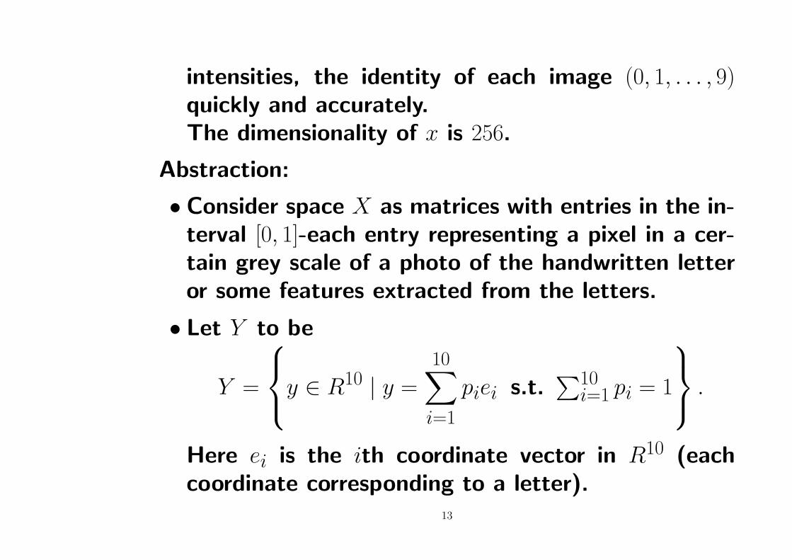
intensities, the identity of each image (0, 1, . . . , 9)quickly and accurately.The dimensionality of x is 256.

Abstraction:

• Consider space X as matrices with entries in the in-terval [0, 1]-each entry representing a pixel in a cer-tain grey scale of a photo of the handwritten letteror some features extracted from the letters.

• Let Y to be

Y =

y ∈ R10 | y =

10∑i=1

piei s.t.∑10

i=1 pi = 1

.

Here ei is the ith coordinate vector in R10 (eachcoordinate corresponding to a letter).

13

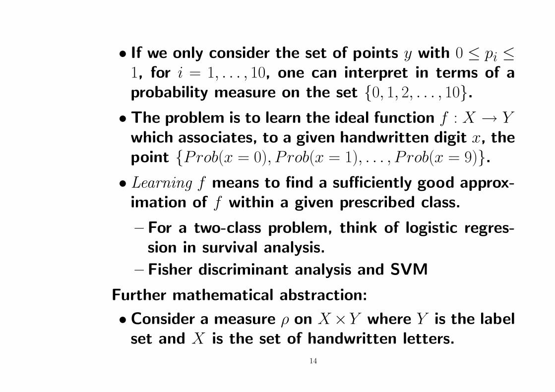
• If we only consider the set of points y with 0 ≤ pi ≤1, for i = 1, . . . , 10, one can interpret in terms of aprobability measure on the set {0, 1, 2, . . . , 10}.

• The problem is to learn the ideal function f : X → Ywhich associates, to a given handwritten digit x, thepoint {Prob(x = 0), P rob(x = 1), . . . , P rob(x = 9)}.

• Learning f means to find a sufficiently good approx-imation of f within a given prescribed class.

– For a two-class problem, think of logistic regres-sion in survival analysis.

– Fisher discriminant analysis and SVM

Further mathematical abstraction:

• Consider a measure ρ on X×Y where Y is the labelset and X is the set of handwritten letters.

14

• The pairs (xi, yi) are randomly drawn from X × Yaccording to the measure ρ.

• yi is a sample for a given xi.

• The function to be learned is the regression functionof fρ.

• fρ(x) is the average of the y values of {x} × Y .

•Difficulty: The probability measure ρ governing thesampling which is not known in advance.

How do we learn f?

15

Prostate Cancer

To identify the risk factors for prostate cancer, Stameyet al. (1989), they examined the correlation betweenthe level of prostate specific antigen (PSA) and a num-ber of clinical and demographic measures, in 97 menwho were about to receive a radical prostatetectomy.

• The goal is to predict the log of PSA (lpsa) from anumber of measurements including log-cancer-volume(lcavol), log prostate weight lweight, age, log ofbenign prostatic hyperplasia amount lbph, seminalvesicle invasion svi, log of capuslar penetration lcp,Gleason score gleason, and percent of Gleason scores4 or 5 pgg45.

• This is a supervised learning problem, known as a re-

16

gression problem, because the outcome measurementis quantitative.

Let Y denote lpsa and X be those explanatory vari-ables.

•We have data in the form of (x1, y1), . . . , (xn, yn).

• Use the squared error loss as the criterion of choos-ing the best prediction function, i.e.,

minθ

E[Y − θ(X)]2.

•What is the θ(·) which minimizes the above least-squares error in population version.

– Find c to minimize E(Y − c)2.

– For every x ∈ X, let E(Y | X = x) be the condi-tional expectation.

17

– Regression function: θ(x) = E(Y | X = x)

– Write Y as the sum of θ(X) and Y − θ(X).

∗ Conditional expectation: E(Y − θ(X) | X) = 0

∗ Conditional variance: V ar(Y | X) = E[(Y −θ(X))2 | X)]

• ANOVA decomposition:

V ar(Y ) = E[V ar(Y | X)] + V ar[E(Y | X)]

– If we use E(Y ) to minimize prediction error E(Y −c)2, its prediction error is V ar(Y ).

– If E(Y | X) is not a constant, the prediction errorof θ(x) is smaller.

•Nonparametric regression: No functional form is as-sumed for θ(·)

18

– Suppose that θ(x) is of the form∑∞

i=1 wiφi(x).

∗What is {φi(x); i = 1, 2, . . .} and how to deter-mine {wi, i = 1, 2, . . .} with finite number of data?

∗ Estimate θ(x) by k-nearest-neighbor method suchas

Y (x) =1

k

∑xi∈Nk(x)

yi,

where Nk(x) is the neighborhood of x defined bythe k closest points xi in the training sample.How do we choose k and Nk(x)?

• Empirical error:

– How do we measure the theoretical error E[Y −f (X)]2?

∗ Consider n examples, {(x1, y1), . . . , (xn, yn)}, in-19

dependently drawn according to ρ.

∗Define the empirical error of f to be

En(f ) =1

n

n∑i=1

(yi − f (xi))2.

What is the empirical cdf?

∗ Is En(f ) close to E[Y − f (X)]2?

∗ Think of the following problem:

Is sample variance a consistent estimate of population variance?

Or the following holds in some sense

1

n

∑i

(yi − y)2 → E(Y − E(Y ))2.

∗ Can we claim that the minimizer f of minf∈F(yi−20

f (xi))2 is close to the minimizer of minf∈F E(Y −

f (X))2?

• Consider the problem of email spam.

– Consider the data which consists of informationfrom 4601 email messages.

– The objective was to design an automatic spamdetector that could filter out spam before cloggingthe users’ mailboxes.

– For all 4601 email messages, the true outcome(email type) email or spam is available, along withthe relative frequencies of 57 of the most com-monly occurring words and punctuation marks inthe email message.

– This is a classification problem.21

DNA Expression Microarrays

DNA is the basic material that make up human chro-mosomes.

• The regulation of gene expression in a cell begins atthe level of transcription of DNA into mRNA.

• Although subsequent processes such as differentialdegradation of mRNA in the cytoplasm and differen-tial translation also regulate the expression of genes,it is of great interest to estimate the relative quan-tities of mRNA species in populations of cells.

• The circumstances under which a particular gene isup- or down-regulated provide important clues aboutgene function.

• The simultaneous expression profiles of many genes22

can provide additional insights into physiological pro-cesses or disease etiology that is mediated by thecoordinated action of sets of genes.

Spotted cDNA microarrays (Brown and Botstein 1999)are emerging as a powerful and cost-effective tool forlarge scale analysis of gene expression.

• In the first step of the technique, samples of DNAclones with known sequence content are spotted andimmobilized onto a glass slide or other substrate, themicroarray.

•Next, pools of mRNA from the cell populations un-der study are purified, reverse-transcribed into cDNA,and labeled with one of two fluorescent dyes, whichwe will refer to as “red” and “green.”

23

• Two pools of differentially labeled cDNA are com-bined and applied to a microarray.

• Labeled cDNA in the pool hybridizes to complemen-tary sequences on the array and any unhybridizedcDNA is washed off.

The result is a few thousand numbers, typically rang-ing from say −6 to 6, measuring the expression levelfor each gene in the target relative to the referencesample. As an example, we have a data set with 64samples (column) and 6830 genes (rows). The chal-lenge is to understand how the genes and samples areorganized. Typical questions are as follows:

•Which samples are most similar to each other, interms of their expression profiles across genes?

24

– Think of the samples as points in 6830-dimensionalspace, which we want to cluster together in someway.

•Which genes are most similar to each other, in termsof their expression profile across samples?

•Do certain genes show very high (or low) expressionfor certain cancer samples?

– Feature selection problem.

25

Statistical Language

For the examples we just described, they have severalcomponents in common.

• For each there is a set of variables that might bedenoted as inputs, which are measured or present.These have some influence on one or more outputs.

• For each example, the goal is to use the inputs topredict the values of the outputs. In machine learn-ing language, this exercise is called supervised learn-ing.

• In statistical literature the inputs are often calledthe predictors or more classically the independent vari-ables.The outputs are called responses, or classically the

26

dependent variables.

• The output can be a quantitative measurement, wheresome measurements are bigger than others, andmeasurements close in value are close in nature.

– EX 1. Consider the famous Iris discrimination ex-amples (Fisher, 1936). In this data set, there are150 cases with 50 cases per class. The output isqualitative (species of Iris) and assumes values in afinite set G = {Virginica, Setosa and Versicolor}.There are four predictors: sepal length, sepal width,petal length, and petal width.

– EX 2. In the handwritten digit example, the out-put is one of 10 different digit class.

– In Ex1 and 2, there is no explicit ordering in the

27

classes, and in fact often descriptive labels ratherthan numbers are used to denote the classes.Qualitative variables are often referred to as cate-gorical or discrete variables as well as factors.

– Ex 3. For given specific atmospheric measurementstoday and yesterday, we want to predict the ozonelevel tomorrow.Given the grayscale values for the pixels of thedigitized image of the handwritten digit, we wantto predict its class labels.

– For all three examples, we think of using the in-puts to predict the output. The distinction inoutput type has led to a naming convention forthe prediction tasks: regression when we predictquantitative outputs, and classification when we

28

predict qualitative outputs.

– For regression and classification, both can be viewedas a task in function approximation.

– For qualitative variables, they are typically repre-sented numerically by codes.

• A third variable type is ordered categorical, such assmall, medium and large, where there is an orderingbetween the values, but no metric notion is appro-priate (the difference between medium and smallneed not be the same as that between large andmedium).

29

IRIS Data

First applied in 1935 by M. Barnard at the suggestionof R.A. Fisher (1936).

• Fisher linear discriminant analysis (FLDA): It con-sists of

– Find linear combination xTa of x = (x1, . . . , xp) tomaximize the the ratio of “between group” and“within group variances.

– xTa is called discriminant variables.

– Predicting the class of an observation x by theclass whose mean vector is closest to x of thediscriminant variables.

– Represent Class k by (µk, Σ).

– Define B0 =∑3

k=1(µk − µ)(µk − µ)T .30

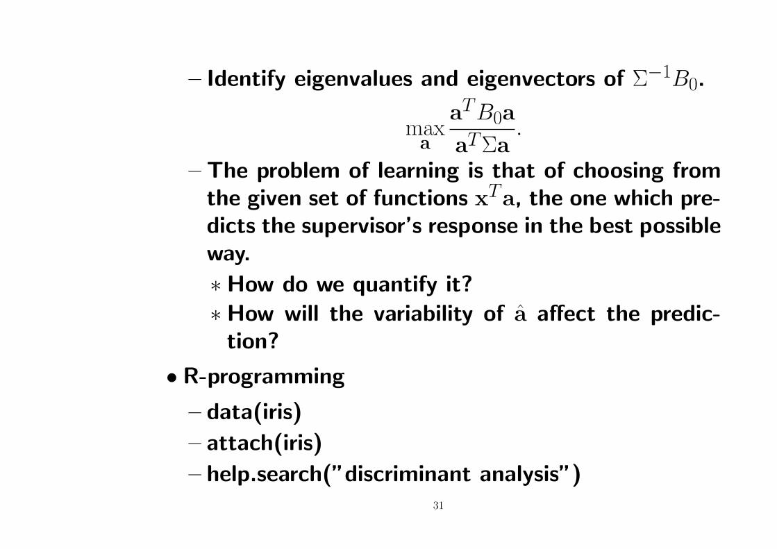
– Identify eigenvalues and eigenvectors of Σ−1B0.

maxa

aTB0a

aTΣa.

– The problem of learning is that of choosing fromthe given set of functions xTa, the one which pre-dicts the supervisor’s response in the best possibleway.

∗How do we quantify it?∗How will the variability of a affect the predic-

tion?

• R-programming

– data(iris)

– attach(iris)

– help.search(”discriminant analysis”)31

– Linear Discriminant Analysis: lda

• Logistic regression

– Model

logP (y = 1 | x)

1− P (y = 1 | x)= α + xTβ

– The coefficients α and β need to be estimatediteratively (writing down the likelihood and findingthe MLE).The “scoring method” or “iterative weighted leastsquares.”

– Convert a classification problem to an estimationproblem.

• Problem of risk minimization

32

– The loss or discrepancy: L(y, f (x|α))Here y is the supervisor’s response to given in-put x and f (x|α) is the response provided by thelearning machine.

– The risk functional: the expected value of the lossor

R(α) =

∫L(y, f (x|α))dρ(x, y).

– Goal: Find the function which minimizes the riskfunctional R(α) (over the class of functions f (x|α),α ∈ A, in the situation where the joint probabil-ity distribution is unknown and the only availableinformation is contained in the training set.

– Pattern recognition

∗ The supervisor’s output y take on only two val-

33

ues {0, 1}.∗ f (x|α), α ∈ A, are a set of indicator functions

the (functions which take on only two valueszero and one).

∗ The loss-function:

L(y, f (x|α)) =

{0 if y = f (x|α),1 if y 6= f (x|α),

∗ For this loss function, the risk functional pro-vides the probability of classification error (i.e.,when the answers given by supervisor and theanswers given by indicator function differ).

∗ The problem, therefore, is to find the functionwhich minimizes the probability of classificationerrors when probability measure is unknown, butthe data are given.

34

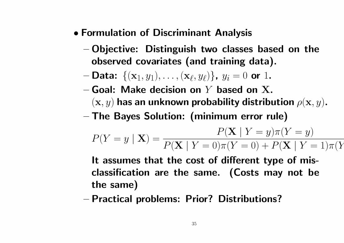
• Formulation of Discriminant Analysis

– Objective: Distinguish two classes based on theobserved covariates (and training data).

– Data: {(x1, y1), . . . , (x`, y`)}, yi = 0 or 1.

– Goal: Make decision on Y based on X.(x, y) has an unknown probability distribution ρ(x, y).

– The Bayes Solution: (minimum error rule)

P (Y = y | X) =P (X | Y = y)π(Y = y)

P (X | Y = 0)π(Y = 0) + P (X | Y = 1)π(Y = 1).

It assumes that the cost of different type of mis-classification are the same. (Costs may not bethe same)

– Practical problems: Prior? Distributions?

35

Role of Optimization in Inference

Many important classes of estimators are defined asthe point at which some function that involves the pa-rameter and the random variable achieves an optimum.

• Estimation by Maximum Likelihood:

– Concept intuitively

– Nice mathematical properties

– Give a sample y1, . . . , yn from a distribution withpdf or pmf p(y | θ∗), MLE of θ is the value thatmaximizes the joint density or joint probabilitywith variable θ at the observed sample value:

∏i p(yi |

θ).

36

• Likelihood function

Ln(θ;y) =

n∏i=1

p(yi | θ).

The value of θ for which Ln achieves its maximumvalue is the MLE of θ∗.

• Critique: How to determine the form of the functionp(y | θ)?

• The data-that is, the realizations of the variables inpdf or pmf- are considered as fixed, and the param-eters are considered as variables of the optimizationproblem,

maxθ

Ln(θ;y).

•Questions:

37

– Does the solution exist?

– Existence of local optima of the objective func-tion.

– Constraints on possible parameter values.

•MLE may not be a good estimation scheme.

• Penalized maximum likelihood estimation

•Optimization in R

– nlm is the general function for “nonlinear mini-mization.”

∗ It can make use of a gradient and/or Hessian,and it can give an estimate of the Hessian atthe minimum.

∗ This function carries out a minimization of thefunction f using a Newton-type algorithm.

38

∗ It needs starting parameter values for the mini-mization.

∗ See demo(nlm) for examples.

– Minimize function of a single variable

∗ optimize: It searches the interval from ’lower’to ’upper’ for a minimum or maximum of thefunction f with respect to its first argument.

∗ uniroot: It searches the interval from ’lower’ to’upper’ for a root of the function f with respectto its first argument.

– D and deriv do symbolic differentiation.

• Example 1: Consider x ∼ mult(n, p) where p = ((2 +θ)/4, (1− θ)/2, θ/4).

– Suppose we observe the data x = (100, 94, 6).

39

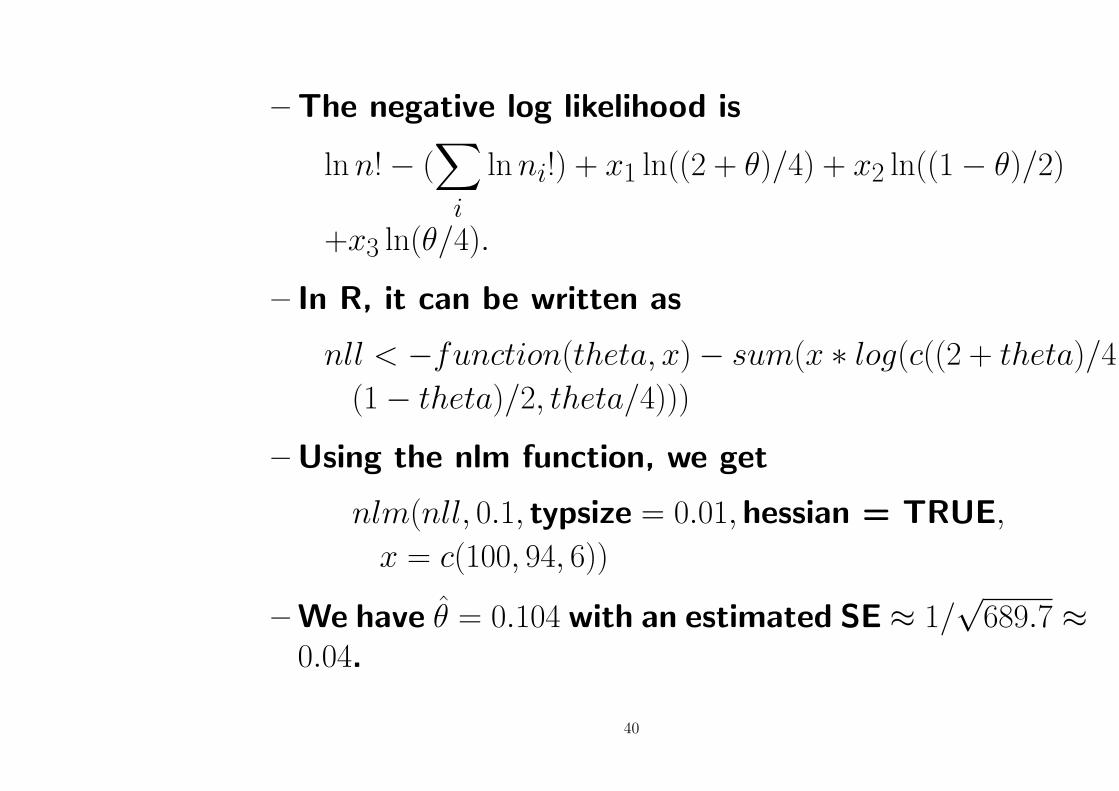
– The negative log likelihood is

ln n!− (∑

i

ln ni!) + x1 ln((2 + θ)/4) + x2 ln((1− θ)/2)

+x3 ln(θ/4).

– In R, it can be written as

nll < −function(theta, x)− sum(x ∗ log(c((2 + theta)/4,

(1− theta)/2, theta/4)))

– Using the nlm function, we get

nlm(nll, 0.1, typsize = 0.01,hessian = TRUE,

x = c(100, 94, 6))

– We have θ = 0.104 with an estimated SE ≈ 1/√

689.7 ≈0.04.

40

EM Methods

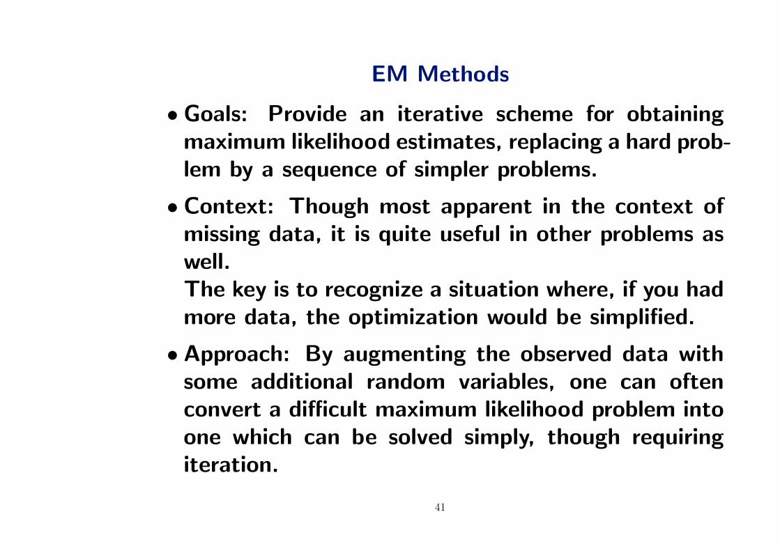
• Goals: Provide an iterative scheme for obtainingmaximum likelihood estimates, replacing a hard prob-lem by a sequence of simpler problems.

• Context: Though most apparent in the context ofmissing data, it is quite useful in other problems aswell.The key is to recognize a situation where, if you hadmore data, the optimization would be simplified.

• Approach: By augmenting the observed data withsome additional random variables, one can oftenconvert a difficult maximum likelihood problem intoone which can be solved simply, though requiringiteration.

41

– Treat the observed data Y as a function Y =Y(X) of a larger set of unobserved complete dataX, in effect treating the density

g(y; θ) =

∫X (y)

f (x; θ)dx.

The trick is to find the right f so that the result-ing maximization is simple, since you will need toiterate the calculation.

• Computational Procedure: The two steps of the cal-culation that give the algorithm its name are

1. Estimate the sufficient statistics of the completedata X given the observed data Y and currentparameter values,

2. Maximize the X-likelihood associated with these42

estimated statistics.

• Genetics Example (Dempster, Laird, and Rubin; 1977):Observe counts

y = (y1, y2, y3, y4) = (125, 18, 20, 34)

∼ Mult(1/2 + θ/4, (1− θ)/4, (1− θ)/4, θ/4)

where 0 ≤ θ ≤ 1.

– Estimate θ by solving the score equationy1

2 + θ− y2 + y3

1− θ+

x4

θ= 0.

It is a quadratic equation in θ.

– Think of y as a collapsed version (y1 = x0 + x1) of

x = (x0, x1, x2, x3, x4) ∼ Mult(1/2, θ/4, (1−θ)/4, (1−θ)/4, θ/4).

43

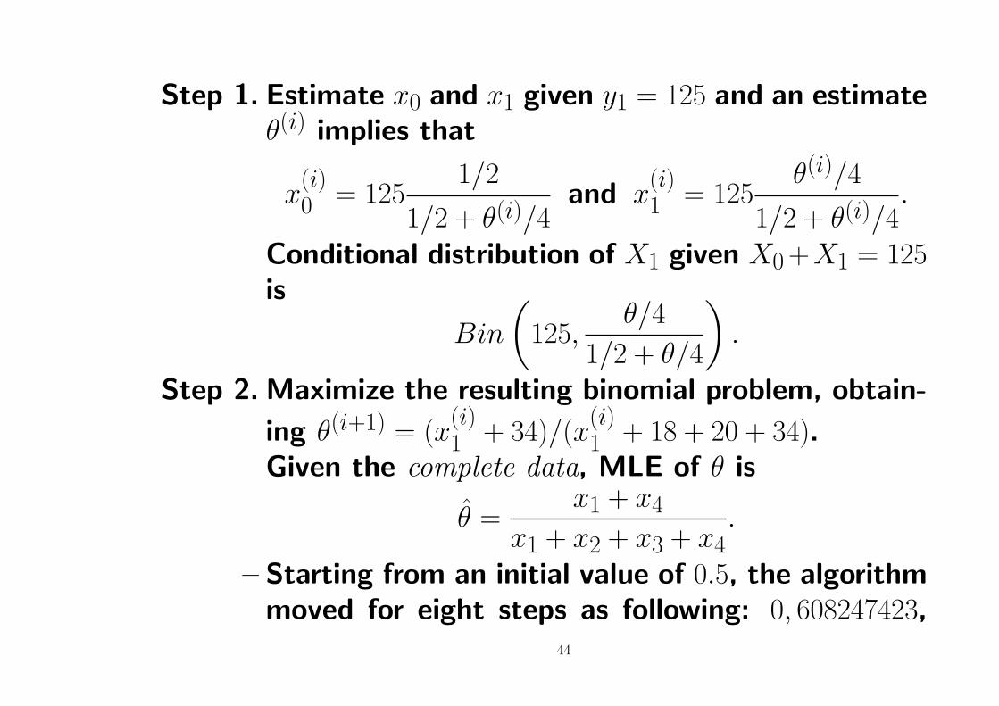
Step 1. Estimate x0 and x1 given y1 = 125 and an estimateθ(i) implies that

x(i)0 = 125

1/2

1/2 + θ(i)/4and x

(i)1 = 125

θ(i)/4

1/2 + θ(i)/4.

Conditional distribution of X1 given X0 +X1 = 125is

Bin

(125,

θ/4

1/2 + θ/4

).

Step 2. Maximize the resulting binomial problem, obtain-

ing θ(i+1) = (x(i)1 + 34)/(x

(i)1 + 18 + 20 + 34).

Given the complete data, MLE of θ is

θ =x1 + x4

x1 + x2 + x3 + x4.

– Starting from an initial value of 0.5, the algorithmmoved for eight steps as following: 0, 608247423,

44

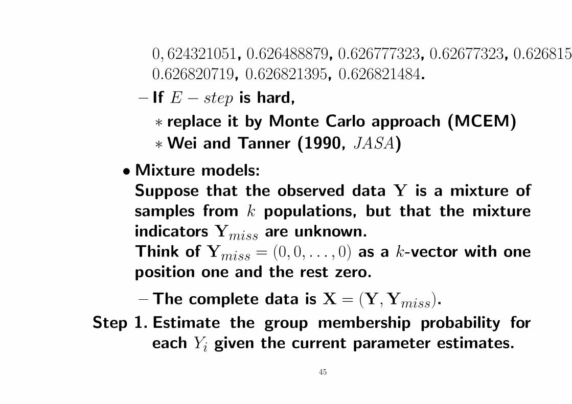
0, 624321051, 0.626488879, 0.626777323, 0.62677323, 0.626815632,0.626820719, 0.626821395, 0.626821484.

– If E − step is hard,

∗ replace it by Monte Carlo approach (MCEM)

∗Wei and Tanner (1990, JASA)

•Mixture models:Suppose that the observed data Y is a mixture ofsamples from k populations, but that the mixtureindicators Ymiss are unknown.Think of Ymiss = (0, 0, . . . , 0) as a k-vector with oneposition one and the rest zero.

– The complete data is X = (Y,Ymiss).

Step 1. Estimate the group membership probability foreach Yi given the current parameter estimates.

45

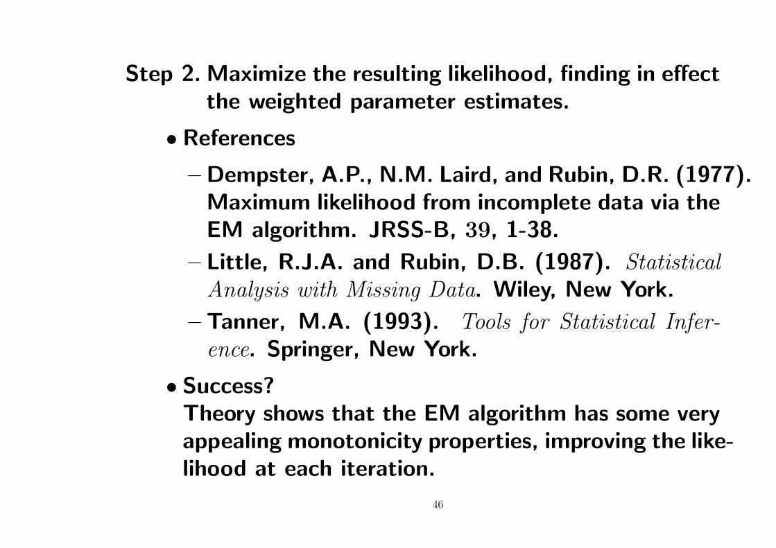
Step 2. Maximize the resulting likelihood, finding in effectthe weighted parameter estimates.

• References

– Dempster, A.P., N.M. Laird, and Rubin, D.R. (1977).Maximum likelihood from incomplete data via theEM algorithm. JRSS-B, 39, 1-38.

– Little, R.J.A. and Rubin, D.B. (1987). StatisticalAnalysis with Missing Data. Wiley, New York.

– Tanner, M.A. (1993). Tools for Statistical Infer-ence. Springer, New York.

• Success?Theory shows that the EM algorithm has some veryappealing monotonicity properties, improving the like-lihood at each iteration.

46

Though often slow to converge, it does get there!

47

EM Methods: Motivating example

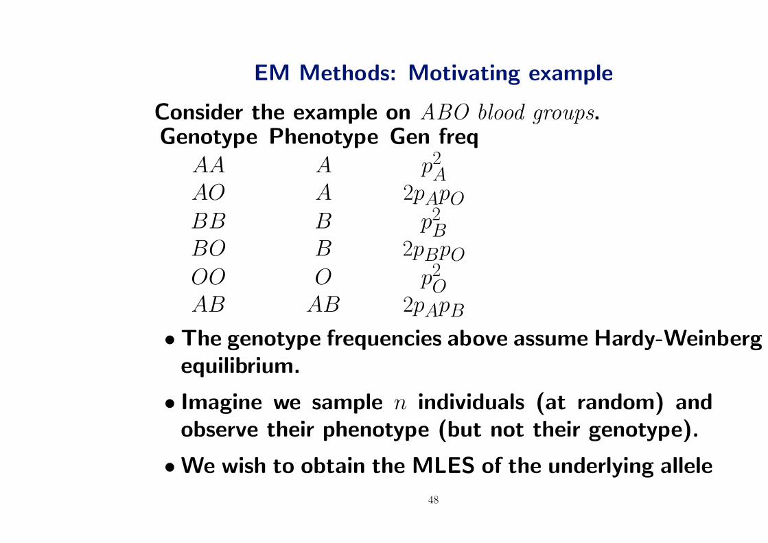
Consider the example on ABO blood groups.Genotype Phenotype Gen freq

AA A p2A

AO A 2pApOBB B p2

BBO B 2pBpOOO O p2

OAB AB 2pApB

• The genotype frequencies above assume Hardy-Weinbergequilibrium.

• Imagine we sample n individuals (at random) andobserve their phenotype (but not their genotype).

•We wish to obtain the MLES of the underlying allele

48

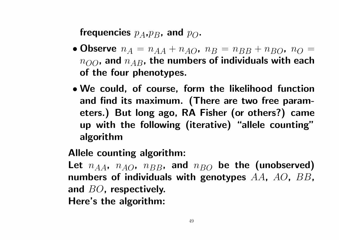
frequencies pA,pB, and pO.

•Observe nA = nAA + nAO, nB = nBB + nBO, nO =nOO, and nAB, the numbers of individuals with eachof the four phenotypes.

•We could, of course, form the likelihood functionand find its maximum. (There are two free param-eters.) But long ago, RA Fisher (or others?) cameup with the following (iterative) “allele counting”algorithm

Allele counting algorithm:Let nAA, nAO, nBB, and nBO be the (unobserved)numbers of individuals with genotypes AA, AO, BB,and BO, respectively.Here’s the algorithm:

49

1. Start with initial estimates p(0) = (p(0)A , p

(0)B , p

(0)O ).

2. Calculate the expected numbers of individuals ineach of the genotype classes, given the observednumbers of individuals in each phenotype class andgiven the current estimates of the allele frequencies.For example:

n(s)AA = E(nAA | nAA, p(s−1))

= nAp(s−1)A /(p

(s−1)A + 2p

(s−1)O ).

3. Get new estimates of the allele frequencies, imagin-

50

ing that the expected n′s were actually observed.

p(s)A = (2n

(s)AA + n

(s)AO + nAB)/n

p(s)B = (2n

(s)BB + n

(s)BO + nAB)/n

p(s)O = (n

(s)AO + n

(s)BO + 2nO)/n.

4. Repeat steps (2) and (3) until the estimate con-verges.

51

EM algorithm

Consider X ∼ f (x | θ) where X = (Xobs, Xmiss) andf (xobs | θ) =

∫f (xobs, xmiss | θ)dxmiss.

•Observe xobs but not xmiss.

•Wish to find the MLE θ = arg maxθ f (xobs | θ).

• In many cases, this can be quite difficult directly,but if we had observed xobs, it would be easy to find

θC = arg maxθ

f (xobs, xmiss | θ).

EM algorithm:

E step:`(s)(θ) = E{log f (xobs, xmiss | θ) | xobs, θ

(s)}

52

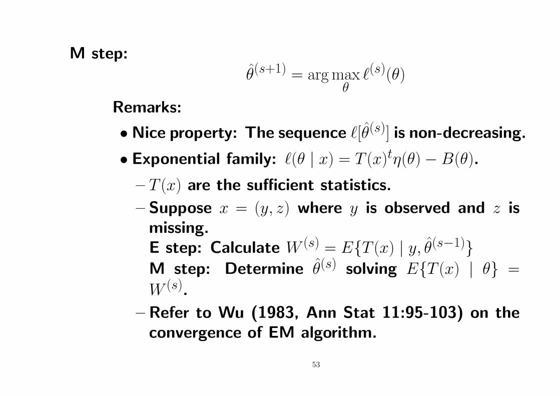
M step:θ(s+1) = arg max

θ`(s)(θ)

Remarks:

•Nice property: The sequence `[θ(s)] is non-decreasing.

• Exponential family: `(θ | x) = T (x)tη(θ)−B(θ).

– T (x) are the sufficient statistics.

– Suppose x = (y, z) where y is observed and z ismissing.E step: Calculate W (s) = E{T (x) | y, θ(s−1)}M step: Determine θ(s) solving E{T (x) | θ} =

W (s).

– Refer to Wu (1983, Ann Stat 11:95-103) on theconvergence of EM algorithm.

53

Normal Mixtures

Finite mixtures are a common modelling technique.

• Suppose that an observable y is represented as nobservations y = (y1, . . . , yn).

• Suppose further that there exists a finite set of Jstates, and that each yi is associated with an unob-served state.Thus, there exists an unobserved vector q = (q1, . . . , qJ),where qi is the indicator vector of length J whosecomponents are all zero except for one equal to unityindicating the unobserved state associated with yi.

•Define the complete data to be x = (y,q).

A natural way to conceptualize mixture specificationsis to think of the marginal distribution of the indicators

54

q, and then to specify the distribution of y given q.

• Assume that the yi given qi are conditionally inde-pendent with densities f (yi | qi).

• Consider x1, . . . , xniid∼

∑Jj=1 pjf (xi | µj, σ) where f (· |

µ, σ) is the normal density.(Here we put the SD rather than the variance here.)

• Let

yij =

{1 if xi is drawn from N(µj, σ)0 otherwise

so that∑

j yij = 1.(xi) is the observed data; (xi, yi) is the completedata.

55

• The following is the unobserved Complete data loglikelihood

`(µ, σ, p | x, y) =∑

i

∑j

yij{log pj + log f (xi | µj, σ)}

– How do we estimate it?

– Sufficient statistics

S1j =∑

i

yij S2j =∑

i

yijxi S3j =∑

i

yijx2i

– E step

w(s)ij = E[yij | xi, p

(s−1), µ(s−1), σ(s−1)]

= Pr[yij = 1 | xi, p(s−1), µ(s−1), σ(s−1)]

=p(s−1)j f (xi | µ

(s−1)j , σ(s−1))∑

j p(s−1)j f (xi | µ

(s−1)j , σ(s−1))

56

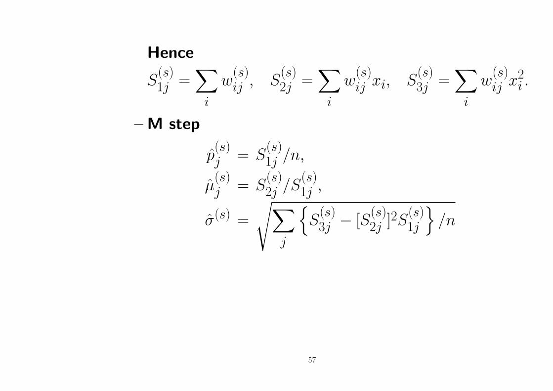
Hence

S(s)1j =

∑i

w(s)ij , S

(s)2j =

∑i

w(s)ij xi, S

(s)3j =

∑i

w(s)ij x2

i .

– M step

p(s)j = S

(s)1j /n,

µ(s)j = S

(s)2j /S

(s)1j ,

σ(s) =

√∑j

{S

(s)3j − [S

(s)2j ]2S

(s)1j

}/n

57

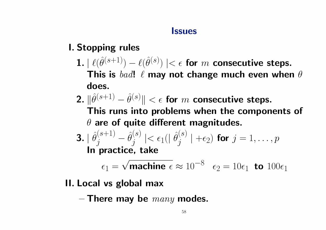
Issues

I. Stopping rules

1. | `(θ(s+1))− `(θ(s)) |< ε for m consecutive steps.This is bad! ` may not change much even when θdoes.

2. ‖θ(s+1) − θ(s)‖ < ε for m consecutive steps.This runs into problems when the components ofθ are of quite different magnitudes.

3. | θ(s+1)j − θ

(s)j |< ε1(| θ

(s)j | +ε2) for j = 1, . . . , p

In practice, take

ε1 =√

machine ε ≈ 10−8 ε2 = 10ε1 to 100ε1

II. Local vs global max

– There may be many modes.58

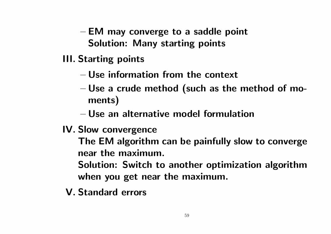
– EM may converge to a saddle pointSolution: Many starting points

III. Starting points

– Use information from the context

– Use a crude method (such as the method of mo-ments)

– Use an alternative model formulation

IV. Slow convergenceThe EM algorithm can be painfully slow to convergenear the maximum.Solution: Switch to another optimization algorithmwhen you get near the maximum.

V. Standard errors

59

– Numerical approximation of the Fisher informa-tion (ie, the Hessian)

– Louis (1982), Meng and Rubin(1991)

60

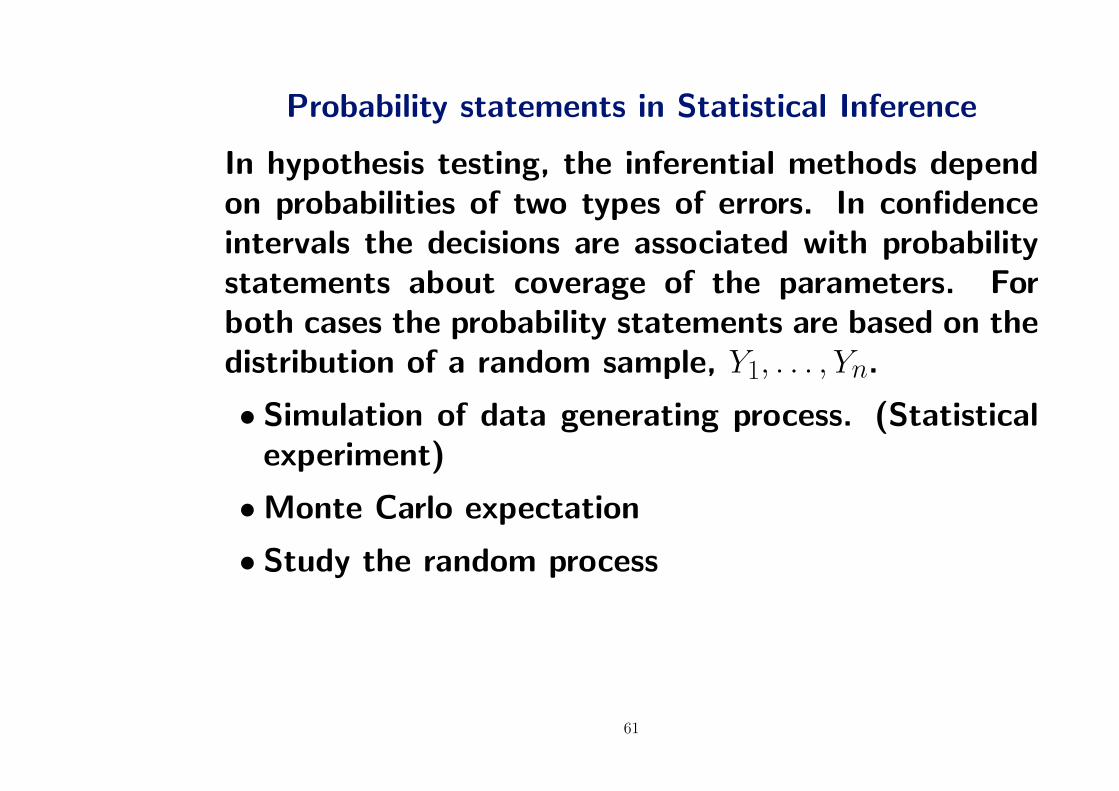
Probability statements in Statistical Inference

In hypothesis testing, the inferential methods dependon probabilities of two types of errors. In confidenceintervals the decisions are associated with probabilitystatements about coverage of the parameters. Forboth cases the probability statements are based on thedistribution of a random sample, Y1, . . . , Yn.

• Simulation of data generating process. (Statisticalexperiment)

•Monte Carlo expectation

• Study the random process

61