Human Learning and Decision Making in a Bandit Setting

Emily Mazo, Zach Fein, Kc Emezie, Eric Gorlin

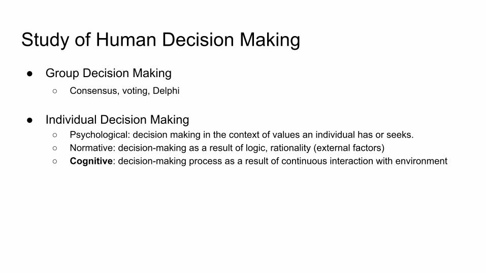
Study of Human Decision Making● Group Decision Making

○ Consensus, voting, Delphi

● Individual Decision Making○ Psychological: decision making in the context of values an individual has or seeks.○ Normative: decision-making as a result of logic, rationality (external factors)○ Cognitive: decision-making process as a result of continuous interaction with environment

Primary Topic

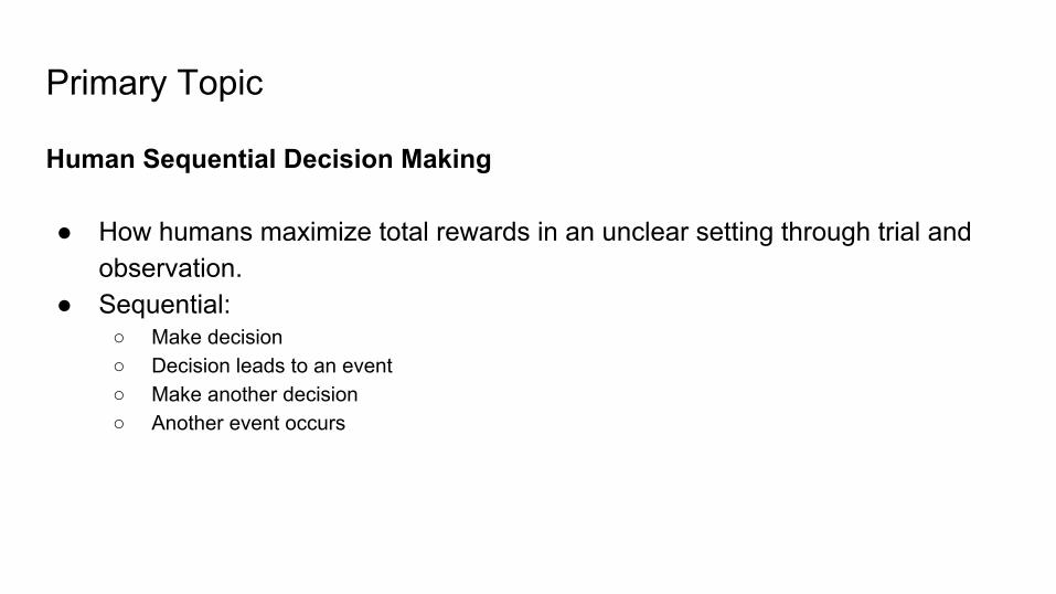
Human Sequential Decision Making

● How humans maximize total rewards in an unclear setting through trial and observation.

● Sequential:○ Make decision○ Decision leads to an event○ Make another decision○ Another event occurs

Prior work Computational modeling of human cognition:

● 1970s: production systems○ Extensive series of rules

● 1980s/1990s: connectionist networks○ Interconnected networks of simple units, dynamic

● Since the 1990s: probabilistic models○ Bayes rule: probability updated with observations

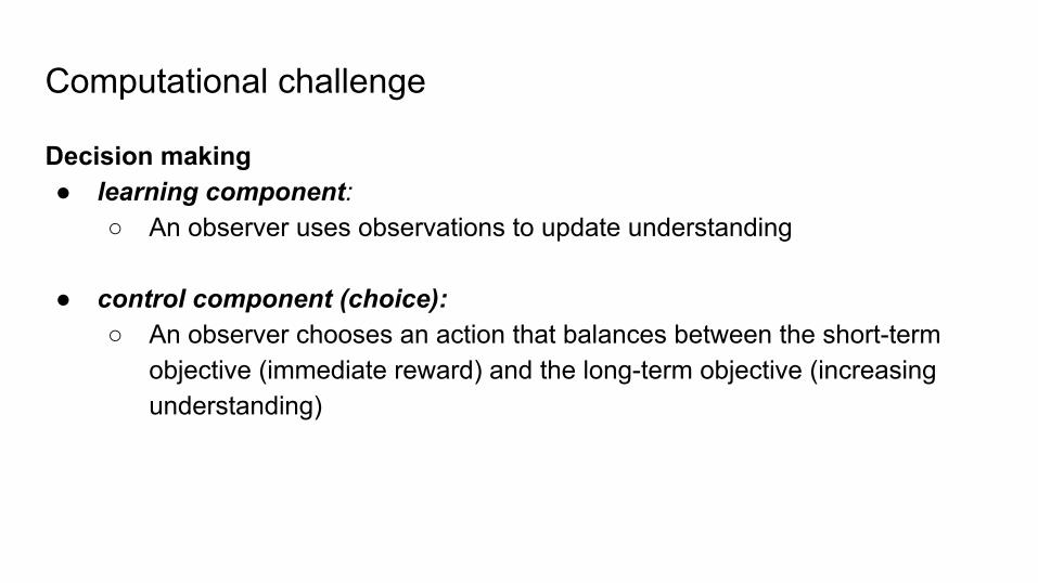
Computational challenge

Decision making● learning component:

○ An observer uses observations to update understanding

● control component (choice): ○ An observer chooses an action that balances between the short-term

objective (immediate reward) and the long-term objective (increasing understanding)

Learning Component

Human Learning Behavior Modeling

● Most models assume that humans:○ Use simple policies that retain little garnered information and/or ignore

long-term optimization

● Popular representation model: Bayesian Learning

Bayesian Learning● Bayes theorem: probability of an event, based on conditions that might be

related to the event.● Dynamic updating of probabilities● Further discussed in Bayesian learning theory applied to human cognition by

Robert A. Jacobs and John K. Kruschke○ “Bayesian models optimally combine information based on prior beliefs with information based

on observations or data”

Control Component

Multi-armed bandit setting● Recall: Multi-armed bandit (As presented in lecture 4 by Connor Lee, Ritvik Mishra, Hoang Le)

○ Gambler has a row of n slot machines○ At each time step t = 0...T, choose a slot machine to plot○ Experiences loss only from the attempted slot machine○ (Gambler) Does not know what would have happened had another slot machine been chosen.○ Objective is to maximize sum of collected rewards

● We define - Standard bandit setting:○ Individuals are given a set # of trials to choose among a set of alternatives (arms) ○ For each choice an outcome is generated based on an unknown reward distribution specific to chosen arm○ Objective: maximize the total reward○ For each trial, reward gained on each trial has an intrinsic value. In addition, reward informs the decision maker about

the relative desirability of the arm -> used with future decisions.

Multi-armed bandit exploration/exploitation

Decision makers have to balance their choices between general exploration (selecting an arm about which one is ignorant) and exploitation (selecting an arm that is known to have relatively high expected reward).

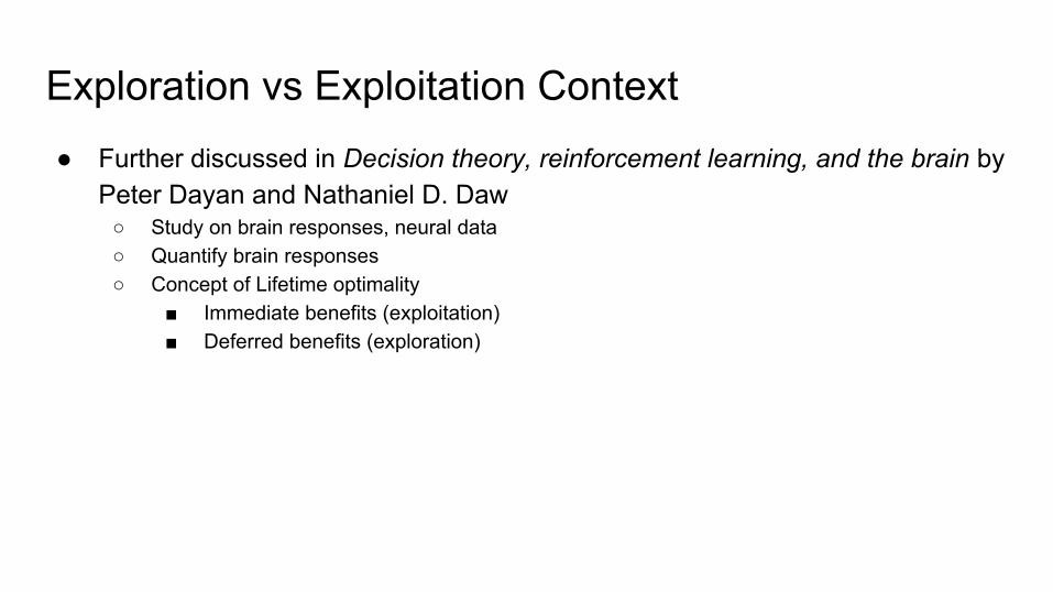
Exploration vs Exploitation Context● Further discussed in Decision theory, reinforcement learning, and the brain by

Peter Dayan and Nathaniel D. Daw○ Study on brain responses, neural data○ Quantify brain responses○ Concept of Lifetime optimality

■ Immediate benefits (exploitation)■ Deferred benefits (exploration)

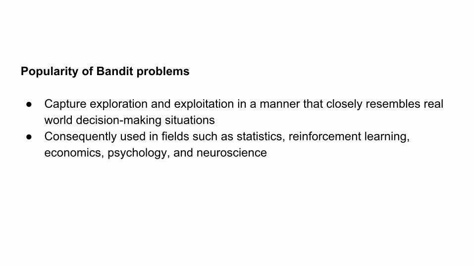
Popularity of Bandit problems

● Capture exploration and exploitation in a manner that closely resembles real world decision-making situations

● Consequently used in fields such as statistics, reinforcement learning, economics, psychology, and neuroscience

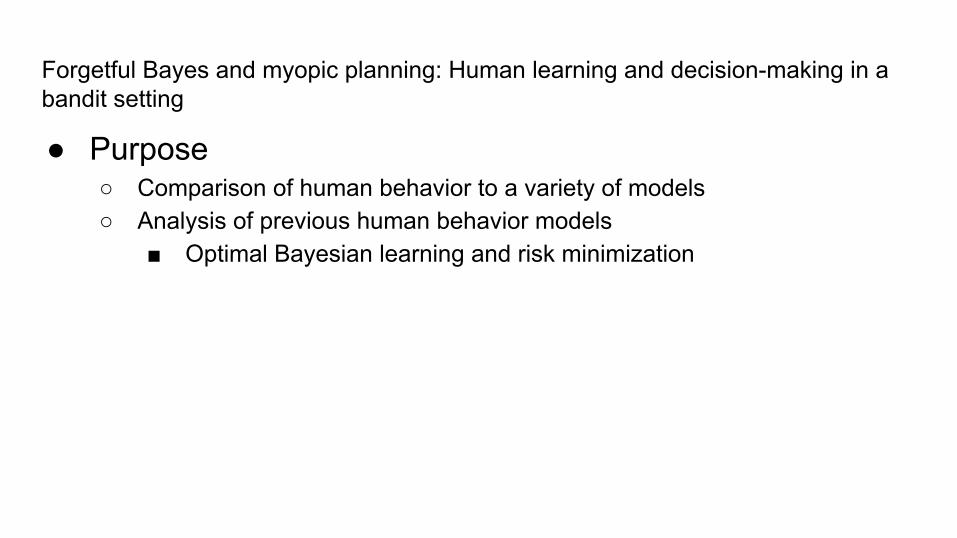
Forgetful Bayes and myopic planning: Human learning and decision-making in a bandit setting

● Purpose○ Comparison of human behavior to a variety of models○ Analysis of previous human behavior models

■ Optimal Bayesian learning and risk minimization

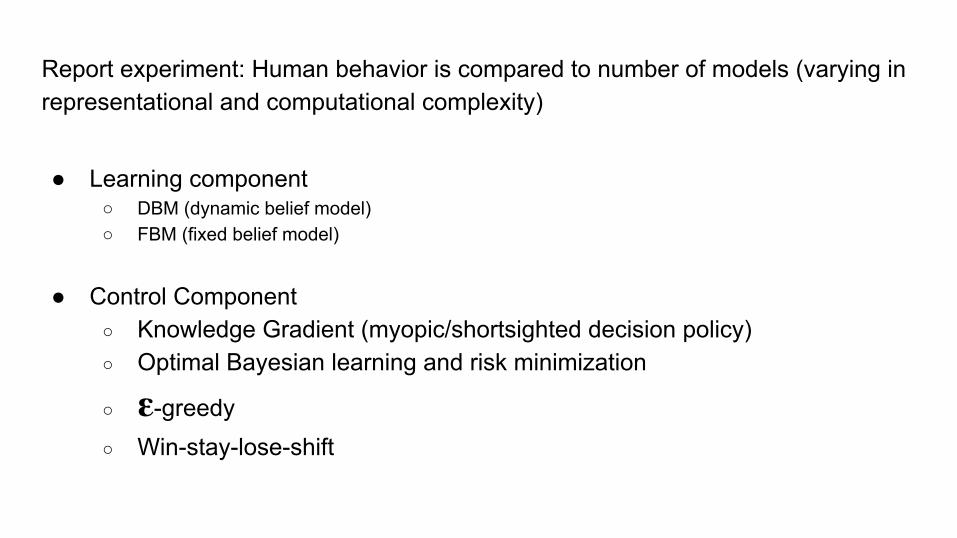
Report experiment: Human behavior is compared to number of models (varying in representational and computational complexity)

● Learning component○ DBM (dynamic belief model)○ FBM (fixed belief model)

● Control Component○ Knowledge Gradient (myopic/shortsighted decision policy)○ Optimal Bayesian learning and risk minimization

○ -greedy○ Win-stay-lose-shift

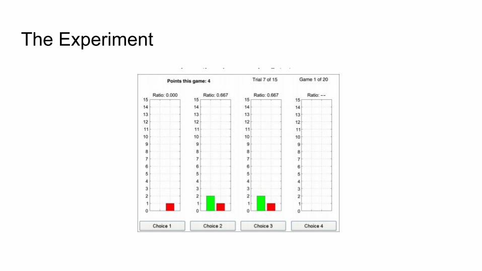
The Experiment

Bayesian Learning in Beta EnvironmentsBayesian Inference: Update your belief about the probability of an event based on new information.

Bayesian Learning: Compute the posterior probability distribution of the target features based on

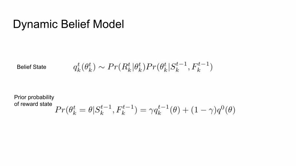
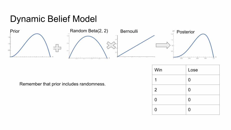
Dynamic Belief Model

Belief State

Prior probability of reward state

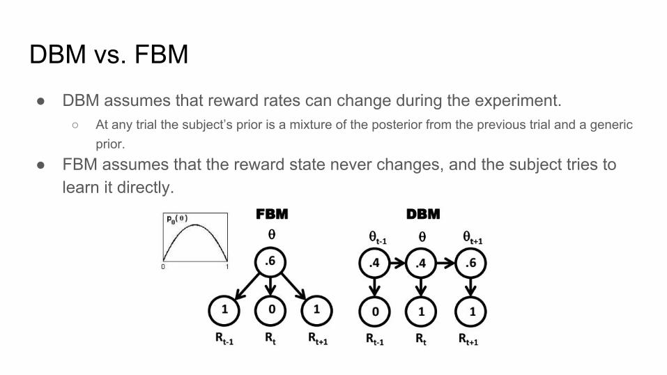
DBM vs. FBM● DBM assumes that reward rates can change during the experiment.

○ At any trial the subject’s prior is a mixture of the posterior from the previous trial and a generic prior.

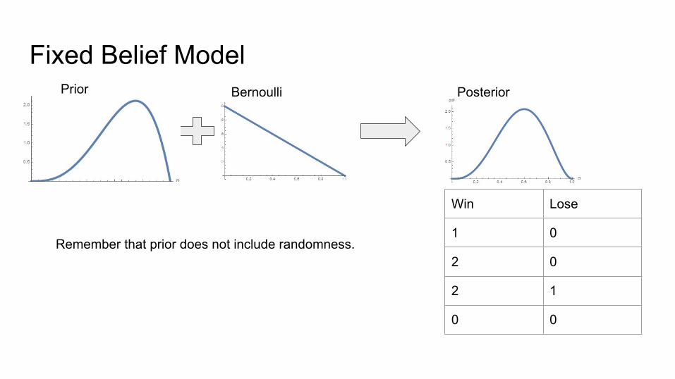
● FBM assumes that the reward state never changes, and the subject tries to learn it directly.

Dynamic Belief Model

Win Lose

0 0

0 0

0 0

0 0

Dynamic Belief Model

Win Lose

1 0

0 0

0 0

0 0

Prior Bernoulli Posterior

Remember that prior includes randomness.

Random Beta(2, 2)

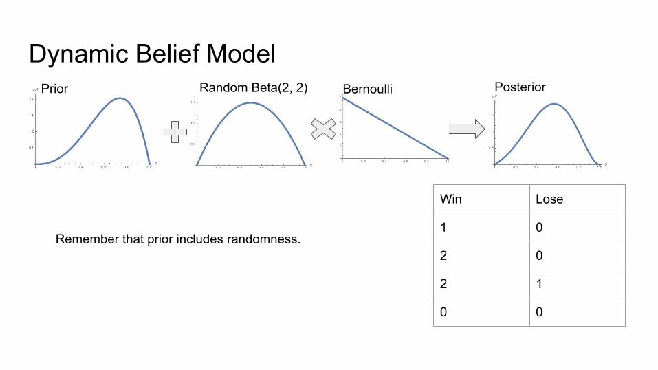
Dynamic Belief Model

Win Lose

1 0

2 0

0 0

0 0

Bernoulli

Remember that prior includes randomness.

Random Beta(2, 2)Prior Posterior

Dynamic Belief Model

Win Lose

1 0

2 0

2 1

0 0

Bernoulli Posterior

Remember that prior includes randomness.

Random Beta(2, 2)Prior

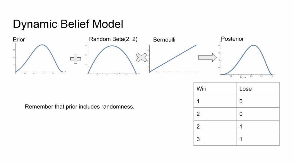
Dynamic Belief Model

Win Lose

1 0

2 0

2 1

3 1

Bernoulli

Remember that prior includes randomness.

Random Beta(2, 2)

0.5

Prior Posterior

Fixed Belief Model

Win Lose

1 0

0 0

0 0

0 0

Bernoulli

Remember that prior does not include randomness.

Prior Posterior

Fixed Belief Model

Win Lose

1 0

2 0

0 0

0 0

Prior Bernoulli Posterior

Remember that prior does not include randomness.

Fixed Belief Model

Win Lose

1 0

2 0

2 1

0 0

Bernoulli Posterior

Remember that prior does not include randomness.

Prior

Fixed Belief Model

Win Lose

1 0

2 0

2 1

3 1

Prior Bernoulli

Remember that prior does not include randomness.

Posterior

Decision Policies

Four models that describe which arm to choose at each trial:

○ Optimal model○ Win-Stay-Lose-Shift○ -greedy○ Knowledge Gradient

Optimal ModelWe can view the problem as a Markov Decision Process with finite horizon and state qt = (q1

t, q2t, q3

t, q4t). This allows us to use Bellman’s equation:

Let Vt(qt) be the expected total future reward at time t. The optimal policy should then follow the recursive reward

Vt(qt) = maxk kt + [Vt+1(qt+1)].

And we choose the optimal decision as

Dt(qt) = argmaxk kt + [Vt+1(qt+1)].

Policy is solved computationally using dynamic programming.

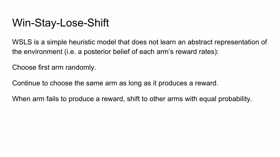
Win-Stay-Lose-ShiftWSLS is a simple heuristic model that does not learn an abstract representation of the environment (i.e. a posterior belief of each arm’s reward rates):

Choose first arm randomly.

Continue to choose the same arm as long as it produces a reward.

When arm fails to produce a reward, shift to other arms with equal probability.

-GreedyParameter controls exploration and exploitation of the arms.

The policy selects arms with the following probability:

Pr(Dt = k | , t) = {where Mt is the number of arms with the largest estimated reward rate at time t.

Policy keeps track of estimated reward rates but not uncertainties or distributions. It plays the same strategy regardless of horizon, always maximizing immediate gain.

(1 - ) / Mt if k ∈ argmaxk’ tk’

/ (K - Mt) otherwise

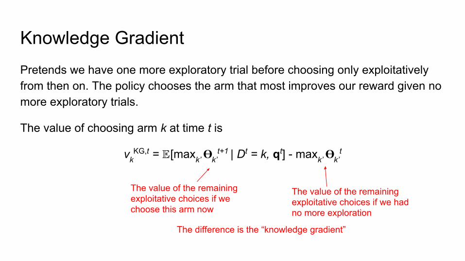
Knowledge GradientPretends we have one more exploratory trial before choosing only exploitatively from then on. The policy chooses the arm that most improves our reward given no more exploratory trials.

The value of choosing arm k at time t is

vkKG,t = [maxk’ k’

t+1 | Dt = k, qt] - maxk’ k’t

The value of the remaining exploitative choices if we choose this arm now

The value of the remaining exploitative choices if we had no more exploration

The difference is the “knowledge gradient”

Knowledge GradientGiven a horizon of T total trials, the decision rule at time t is

DKG, t = argmaxk [ kt + (T - t - 1) vk

KG,t ]

The expected immediate reward of arm k

The total expected knowledge gain on the (T - t - 1) exploitative choices after this exploratory trial

The KG policy will explore more early and exploit more later on.

ExampleAt trial t = 12:

T = 100 Arm 1 Arm 2 Arm 3 Arm 4

Wins 3 1 0 2

Losses 1 2 2 0

Expected Reward Rate * under DBM

0.64 0.41 0.35 0.65

Choose Arm 1 (D12 = 1)

ExampleArm 1 returns success

T = 100 Arm 1 Arm 2 Arm 3 Arm 4

Wins 4 1 0 2

Losses 1 2 2 0

Expected Reward Rate * under DBM

0.67 0.41 0.35 0.65

ExampleAt time t = 13:

T = 100 Arm 1 Arm 2 Arm 3 Arm 4

Wins 4 1 0 2

Losses 1 2 2 0

Expected Reward Rate 0.67 0.41 0.35 0.65

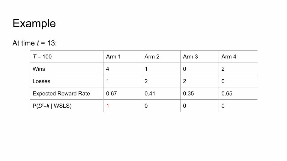
ExampleAt time t = 13:

T = 100 Arm 1 Arm 2 Arm 3 Arm 4

Wins 4 1 0 2

Losses 1 2 2 0

Expected Reward Rate 0.67 0.41 0.35 0.65

P(Dt=k | WSLS) 1 0 0 0

ExampleAt time t = 13:

T = 100 Arm 1 Arm 2 Arm 3 Arm 4

Wins 4 1 0 2

Losses 1 2 2 0

Expected Reward Rate 0.67 0.41 0.35 0.65

P(Dt=k | WSLS) 1 0 0 0

P(Dt=k | -greedy) 1 - / 3 / 3 / 3

ExampleAt time t = 13:

T = 100 Arm 1 Arm 2 Arm 3 Arm 4

Wins 4 1 0 2

Losses 1 2 2 0

Expected Reward Rate 0.67 0.41 0.35 0.65

P(Dt=k | WSLS) 1 0 0 0

P(Dt=k | -greedy) 1 - / 3 / 3 / 3

vkKG,t 0.009 0 0 0.011

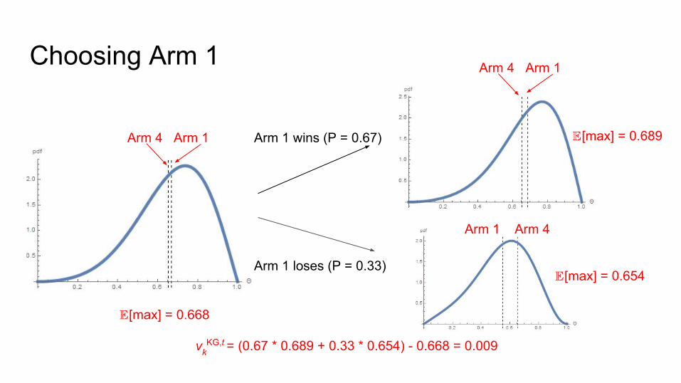
Choosing Arm 1

Arm 4 Arm 1

Arm 1 loses (P = 0.33)

Arm 1 wins (P = 0.67)

Arm 4 Arm 1

Arm 1 Arm 4

[max] = 0.689

[max] = 0.668

[max] = 0.654

vkKG,t = (0.67 * 0.689 + 0.33 * 0.654) - 0.668 = 0.009

Choosing Arm 4

Arm 4 Arm 1

Arm 4 loses (P = 0.35)

Arm 4 wins (P = 0.65)

Arm 1 Arm 4

Arm 4 Arm 1

[max] = 0.685

[max] = 0.668

[max] = 0.668

vkKG,t = (0.65 * 0.685 + 0.35 * 0.668) - 0.668 = 0.011

ExampleAt time t = 13:At time t = 13:

T = 100 Arm 1 Arm 2 Arm 3 Arm 4

Wins 4 1 0 2

Losses 1 2 2 0

Expected Reward Rate 0.67 0.41 0.35 0.65

P(Dt=k | WSLS) 1 0 0 0

P(Dt=k | -greedy) 1 - / 3 / 3 / 3

vkKG,t 0.009 0 0 0.011

kt + (T - t - 1) vk

KG,t 1.48 0.41 0.35 1.62

Model Inference and EvaluationModel agreement with human behavior is measured trial-by-trial based on likelihood of choices given each model.

Markov Chain Monte Carlo techniques were used to sample the posterior distributions of and (Beta priors), (DBM policy coefficient), and (as in -greedy).

Models were fit among all subjects, and average per-trial likelihood was calculated based on the maximum a posteriori estimates of the distributions above.

Model Agreement with Optimal Policy● Graph shows likelihood of model generating

data simulated by optimal model● Win-stay-lose-shift: over 60% agreement with

optimal despite simplicity○ Because optimal model rarely shifts after a win○ Errors arise when switching from a good arm late in trial

● Epsilon-greedy does well● Knowledge Gradient does even better

○ Unsurprising- it’s an approximation of optimal model

● Fixed vs dynamic belief model doesn’t matter○ Optimal policy knows true environment○ Internal belief won’t need change

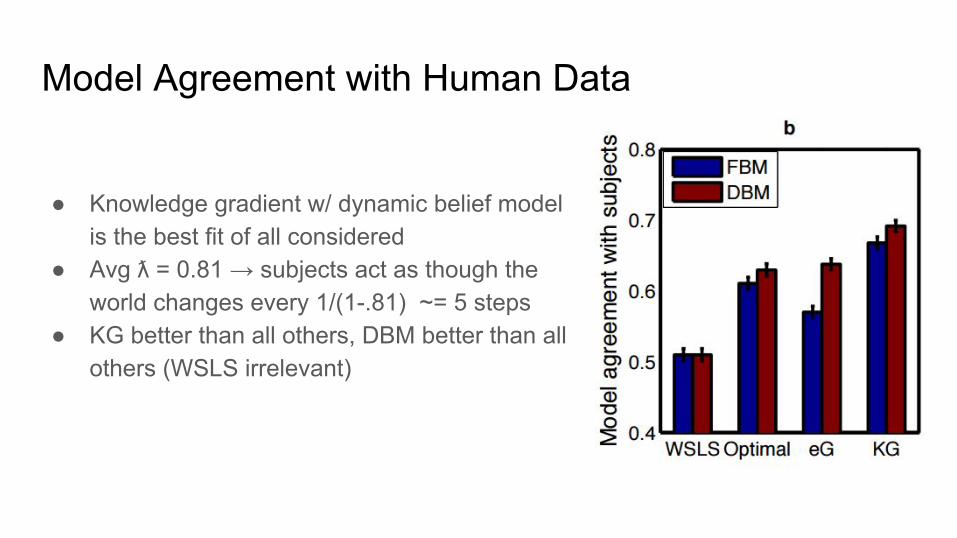
Model Agreement with Human Data

● Knowledge gradient w/ dynamic belief model is the best fit of all considered

● Avg ƛ = 0.81 → subjects act as though the world changes every 1/(1-.81) ~= 5 steps

● KG better than all others, DBM better than all others (WSLS irrelevant)

Individually Fit Model Agreement with Human Data

● Models also trained per person, not overall○ Each have own beta prior and ƛ

● Fit better, pattern remains: KG > eG○ But not by much

● DBM helps eG a lot

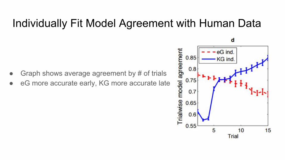
Individually Fit Model Agreement with Human Data

● Graph shows average agreement by # of trials● eG more accurate early, KG more accurate late

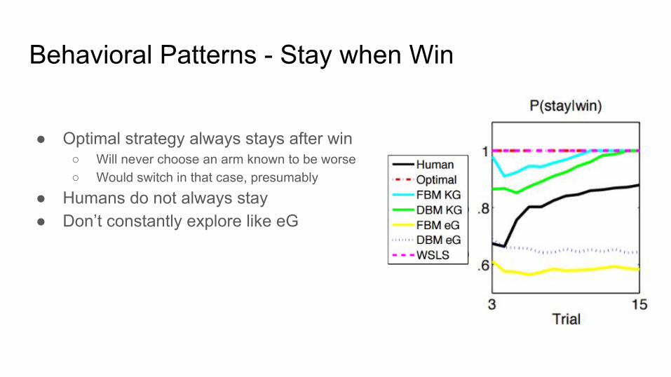
Behavioral Patterns - Stay when Win

● Optimal strategy always stays after win○ Will never choose an arm known to be worse○ Would switch in that case, presumably

● Humans do not always stay● Don’t constantly explore like eG

Behavioral Patterns - Shift when Lose

● Important to trend downward from exploration to exploitation near end

● All algorithms except for WSLS do this● eG with DBM mimics humans the most

○ But not by much

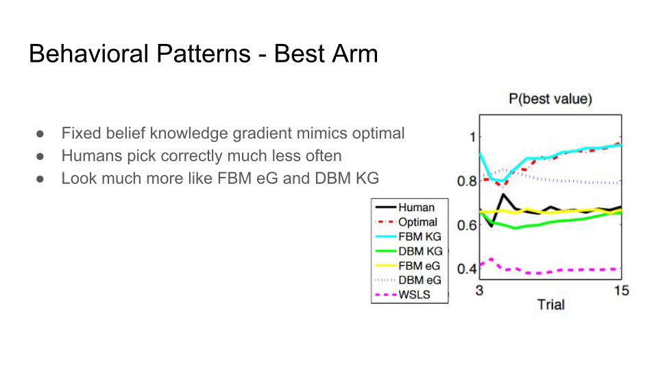
Behavioral Patterns - Best Arm

● Fixed belief knowledge gradient mimics optimal● Humans pick correctly much less often● Look much more like FBM eG and DBM KG

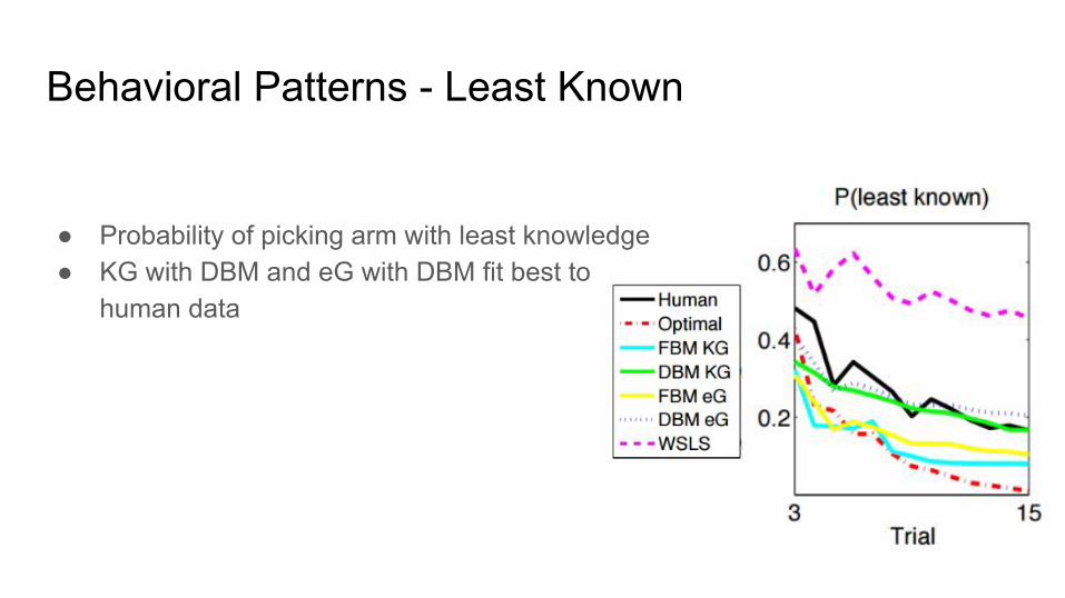
Behavioral Patterns - Least Known

● Probability of picking arm with least knowledge● KG with DBM and eG with DBM fit best to

human data

Caveats● Should not conclude that humans definitely solve bandit problems via a

knowledge gradient with a dynamic belief model○ Limited set of models were tested

● Just people taking artificial tests. Does it reflect a true decision process?○ Did anybody actually try very hard on the Caltech Cohort Study?○ Maybe lack of effort isolates intuition?

Evolutionary Insights● Observed behavior matches best cheap approximation of optimal algorithm● People acted as if rewards were not constant even when told otherwise● These may not be coincidences- sounds like evolution● Bandit-style problems common in nature (e.g. where to look for food today?)● Real world is constantly changing, requires adaptive decision processes● Expensive solutions cost more than they help, especially in online settings

○ Real life is an online setting○ Human mind full of good approximations and heuristics (e.g. gut feels, intuition, emotion)

● This is just speculation!

Applications/Further WorkDecision Making in a Bandit Setting:

● Economics:○ J. Banks, M. Olson, and D. Porter. An experimental analysis of the bandit problem. Economic

Theory■ Always myopic vs never myopic behavior

● Psychology and Neuroscience:○ M. D. Lee, S. Zhang, M. Munro, and M. Steyvers. Psychological models of human and optimal

performance in bandit problems■ latent state modeling: behavior is treated as a mixture of different processes■ Win-stay lose-shift, e-greedy, e-decreasing

● Technology○ http://research.microsoft.com/en-us/projects/bandits/

Applications/Further Work (continued)Different Approach:

● Human Behavior Modeling with Maximum Entropy Inverse Optimal Control Brian D. Ziebart, Andrew Maas, J.Andrew Bagnell, and Anind K. Dey

○ Markov Decision Process framework○ Context-sensitive decisions: Human decision making is goal oriented○ Analysis of behavior of taxi-driver

■ Goal oriented decision making■ Modeling matched routes with ~75 % accuracy

○ Analysis of daily activities of individuals

Questions?