


Hidden Markov Models - UMIACShal/courses/2011F_ML/out/hmms-sl.pdf · With prob. 1-c, follow a...
40
CS 726: HMMs 1 Hal Daumé III ([email protected]) Hidden Markov Models CS 726 Machine Learning Fall 2011 Hal Daumé III [email protected] Many slides courtesy of Dan Klein, Stuart Russell, or Andrew Moore
Transcript of Hidden Markov Models - UMIACShal/courses/2011F_ML/out/hmms-sl.pdf · With prob. 1-c, follow a...

CS 726: HMMs1 Hal Daumé III ([email protected])
Hidden Markov Models
CS 726Machine Learning
Fall 2011
Hal Daumé [email protected]
Many slides courtesy ofDan Klein, Stuart Russell,
or Andrew Moore
CS 726: HMMs2 Hal Daumé III ([email protected])
Reasoning over Time
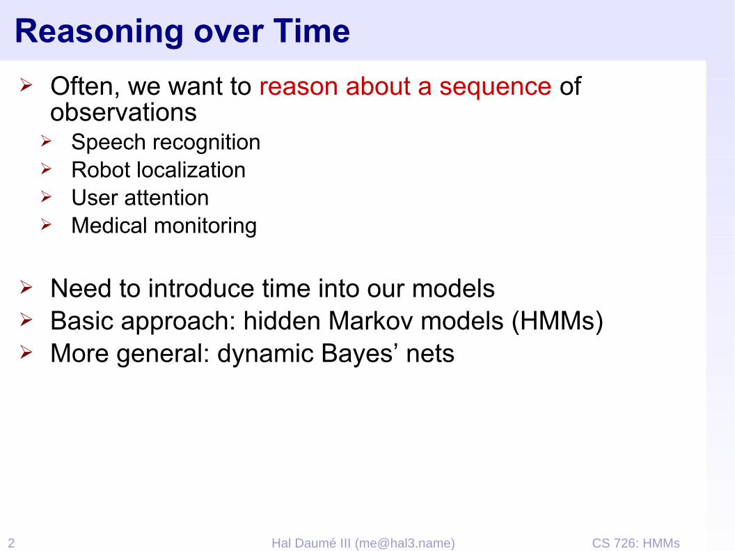
➢ Often, we want to reason about a sequence of observations
➢ Speech recognition➢ Robot localization➢ User attention➢ Medical monitoring
➢ Need to introduce time into our models➢ Basic approach: hidden Markov models (HMMs)➢ More general: dynamic Bayes’ nets
CS 726: HMMs3 Hal Daumé III ([email protected])
Markov Models
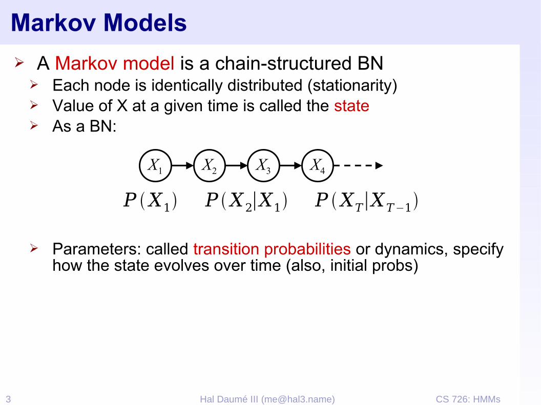
➢ A Markov model is a chain-structured BN➢ Each node is identically distributed (stationarity)➢ Value of X at a given time is called the state➢ As a BN:
➢ Parameters: called transition probabilities or dynamics, specify how the state evolves over time (also, initial probs)
X2X1 X3 X4
P X1 P X2∣X1 P XT∣XT−1
CS 726: HMMs4 Hal Daumé III ([email protected])
Conditional Independence
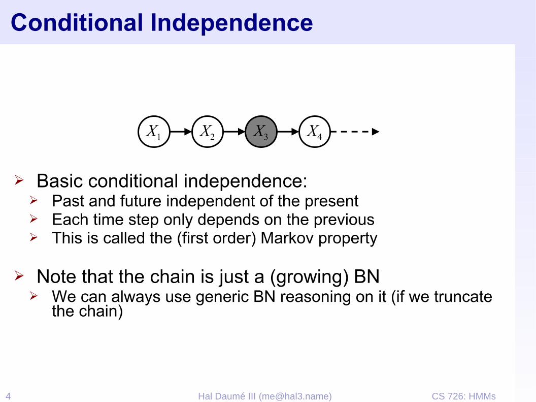
➢ Basic conditional independence:➢ Past and future independent of the present➢ Each time step only depends on the previous➢ This is called the (first order) Markov property
➢ Note that the chain is just a (growing) BN➢ We can always use generic BN reasoning on it (if we truncate
the chain)
X2X1 X3 X4

CS 726: HMMs5 Hal Daumé III ([email protected])
Example: Markov Chain
➢ Weather:➢ States: X = {rain, sun}➢ Transitions:
➢ Initial distribution: 1.0 sun➢ What’s the probability distribution after one step?
rain sun
0.9
0.9
0.1
0.1
This is a CPT, not a BN!
CS 726: HMMs6 Hal Daumé III ([email protected])
Mini-Forward Algorithm
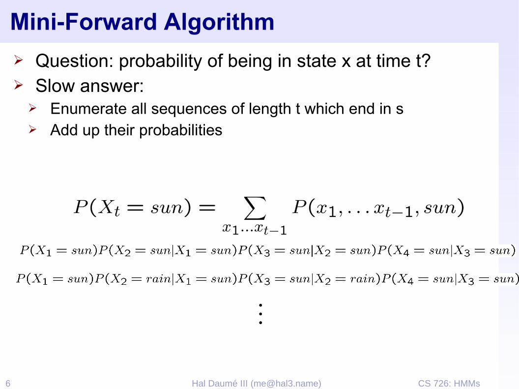
➢ Question: probability of being in state x at time t?➢ Slow answer:
➢ Enumerate all sequences of length t which end in s➢ Add up their probabilities
…
CS 726: HMMs7 Hal Daumé III ([email protected])
Mini-Forward Algorithm
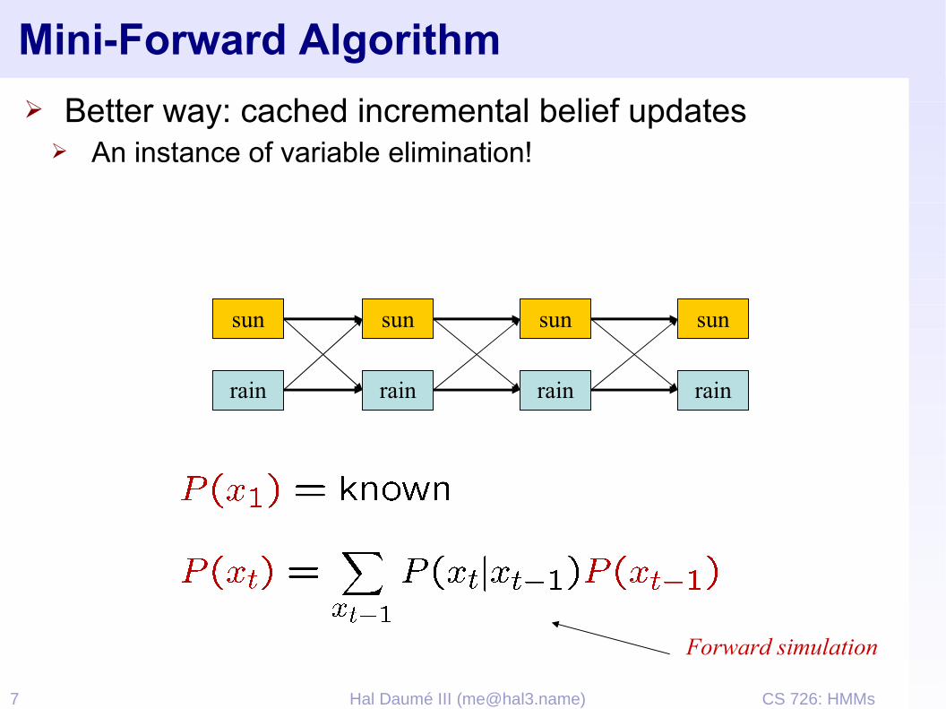
➢ Better way: cached incremental belief updates➢ An instance of variable elimination!
sun
rain
sun
rain
sun
rain
sun
rain
Forward simulation
CS 726: HMMs8 Hal Daumé III ([email protected])
Example
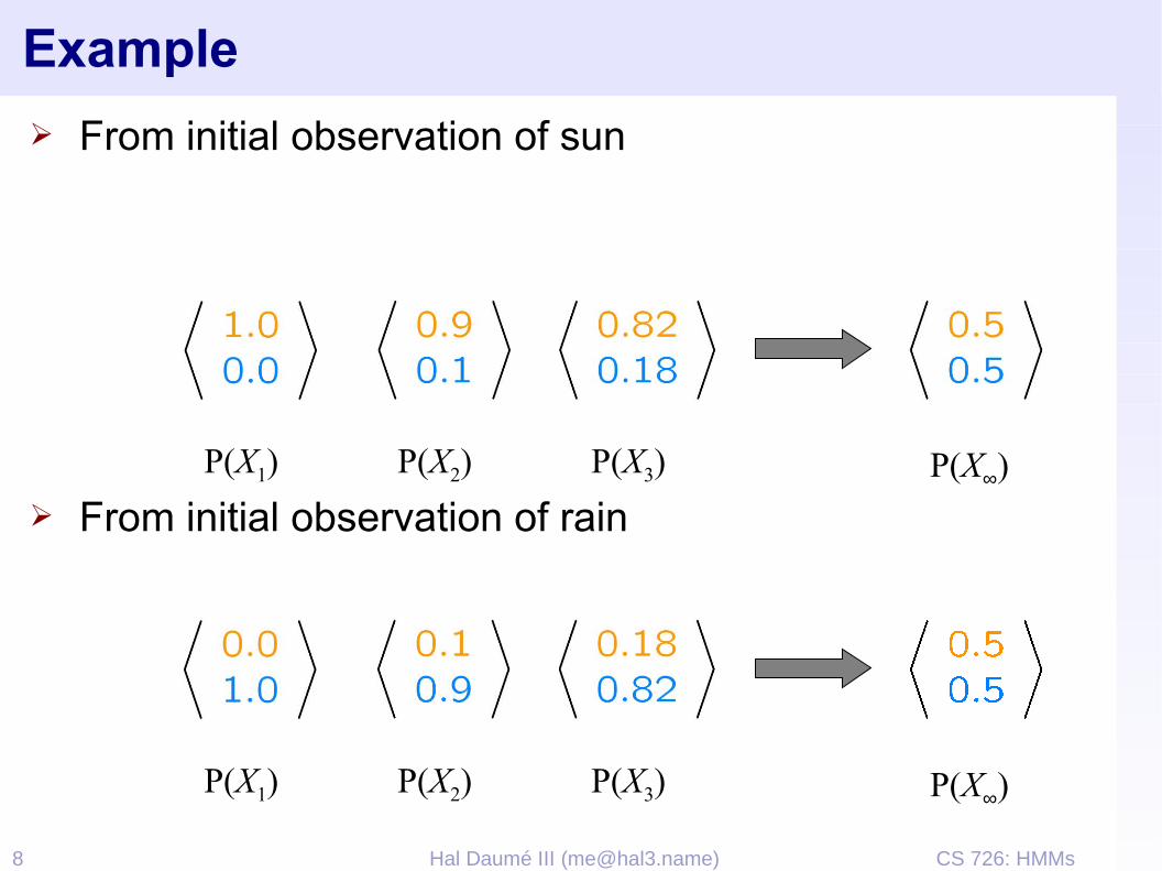
➢ From initial observation of sun
➢ From initial observation of rain
P(X1) P(X2) P(X3) P(X∞)
P(X1) P(X2) P(X3) P(X∞)

CS 726: HMMs9 Hal Daumé III ([email protected])
Stationary Distributions
➢ If we simulate the chain long enough:➢ What happens?➢ Uncertainty accumulates➢ Eventually, we have no idea what the state is!
➢ Stationary distributions:➢ For most chains, the distribution we end up in is independent of
the initial distribution (but not always uniform!)➢ Called the stationary distribution of the chain➢ Usually, can only predict a short time out
CS 726: HMMs10 Hal Daumé III ([email protected])
Web Link Analysis
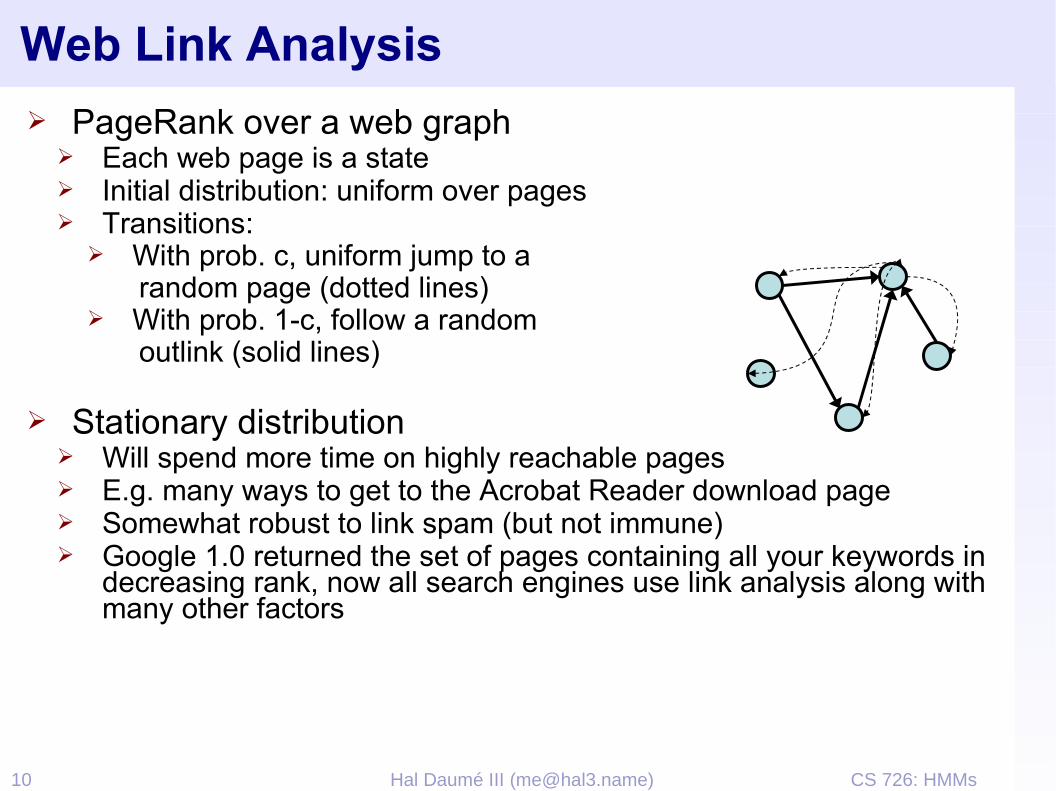
➢ PageRank over a web graph➢ Each web page is a state➢ Initial distribution: uniform over pages➢ Transitions:
➢ With prob. c, uniform jump to arandom page (dotted lines)
➢ With prob. 1-c, follow a randomoutlink (solid lines)
➢ Stationary distribution➢ Will spend more time on highly reachable pages➢ E.g. many ways to get to the Acrobat Reader download page➢ Somewhat robust to link spam (but not immune)➢ Google 1.0 returned the set of pages containing all your keywords in
decreasing rank, now all search engines use link analysis along with many other factors
CS 726: HMMs11 Hal Daumé III ([email protected])
Hidden Markov Models
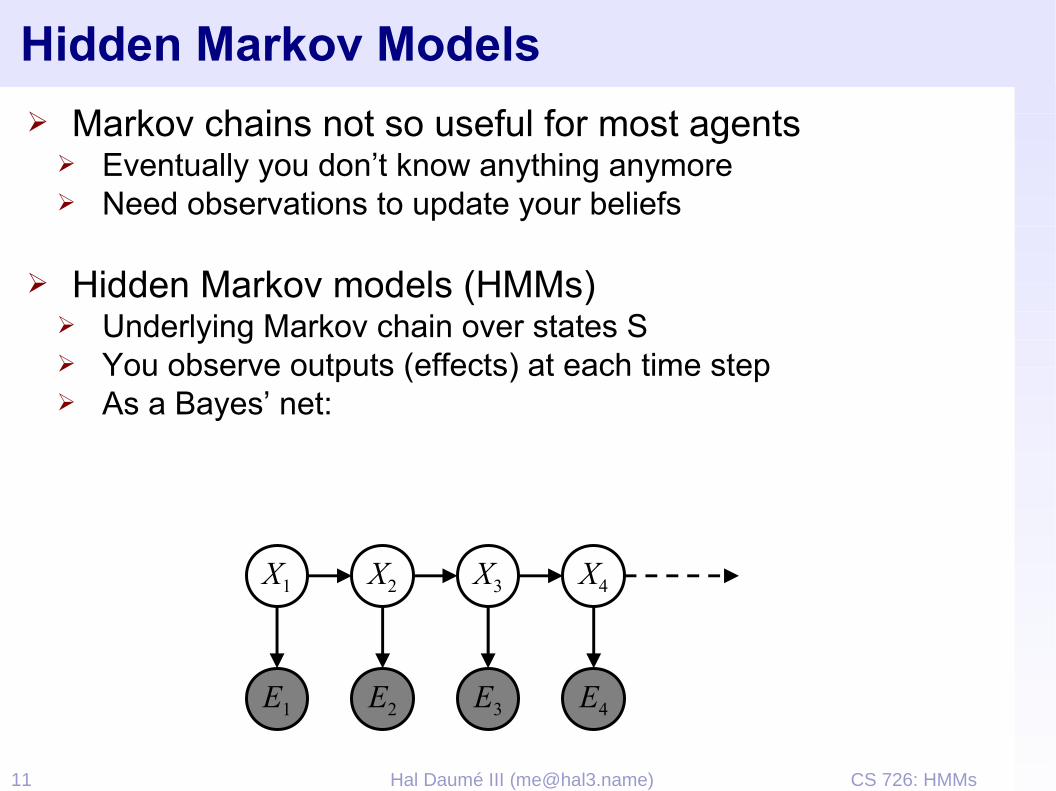
➢ Markov chains not so useful for most agents➢ Eventually you don’t know anything anymore➢ Need observations to update your beliefs
➢ Hidden Markov models (HMMs)➢ Underlying Markov chain over states S➢ You observe outputs (effects) at each time step➢ As a Bayes’ net:
X5X2
E1
X1 X3 X4
E2 E3 E4 E5
CS 726: HMMs12 Hal Daumé III ([email protected])
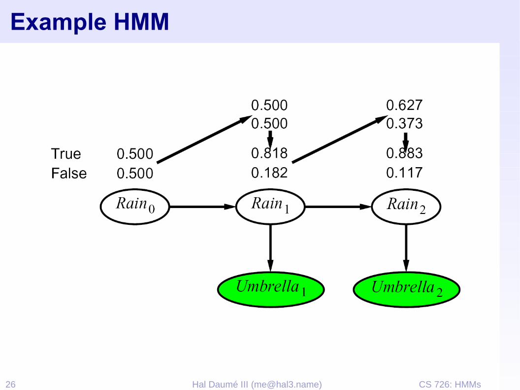
Example
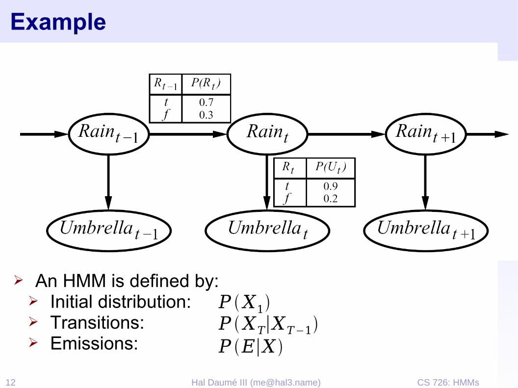
➢ An HMM is defined by:➢ Initial distribution:➢ Transitions:➢ Emissions:
P X1P XT∣XT−1
P E∣X
CS 726: HMMs13 Hal Daumé III ([email protected])
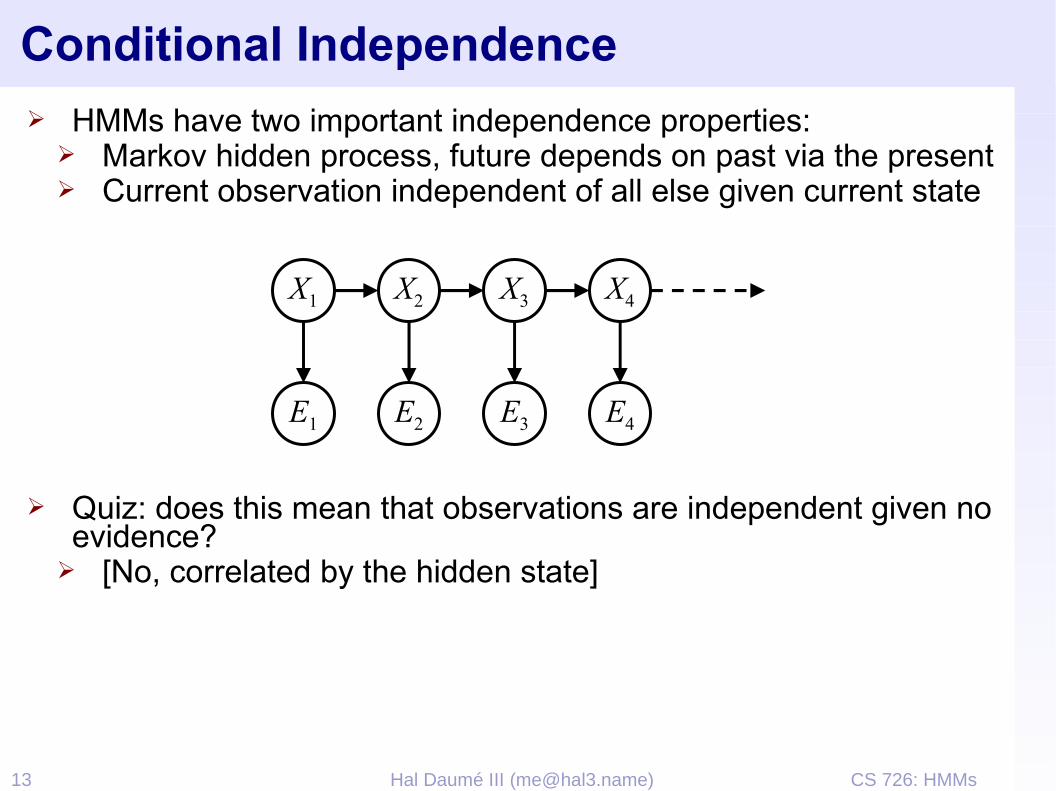
Conditional Independence➢ HMMs have two important independence properties:
➢ Markov hidden process, future depends on past via the present➢ Current observation independent of all else given current state
➢ Quiz: does this mean that observations are independent given no evidence?
➢ [No, correlated by the hidden state]
X5X2
E1
X1 X3 X4
E2 E3 E4 E5
CS 726: HMMs14 Hal Daumé III ([email protected])
Real HMM Examples➢ Speech recognition HMMs:
➢ Observations are acoustic signals (continuous valued)➢ States are specific positions in specific words (so, tens of
thousands)
➢ Machine translation HMMs:➢ Observations are words (tens of thousands)➢ States are translation options
➢ Robot tracking:➢ Observations are range readings (continuous)➢ States are positions on a map (continuous)

CS 726: HMMs15 Hal Daumé III ([email protected])
Filtering / Monitoring➢ Filtering, or monitoring, is the task of tracking the distribution B(X)
(the belief state)➢ We start with B(X) in an initial setting, usually uniform➢ As time passes, or we get observations, we update B(X)
CS 726: HMMs16 Hal Daumé III ([email protected])
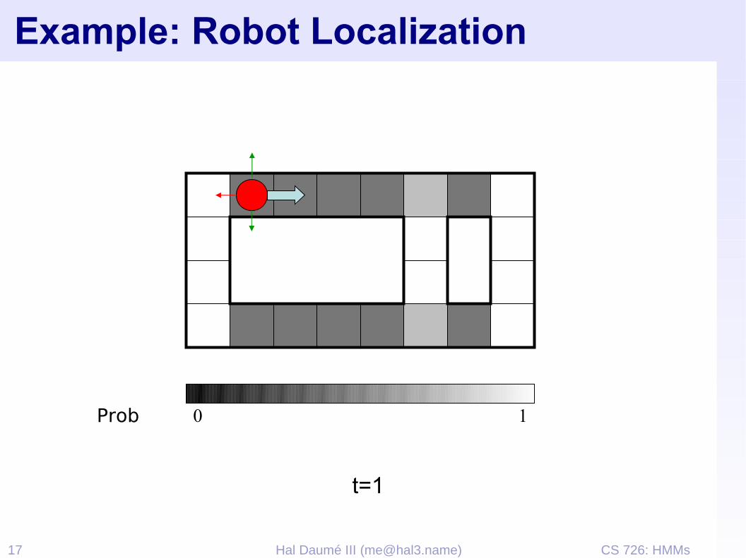
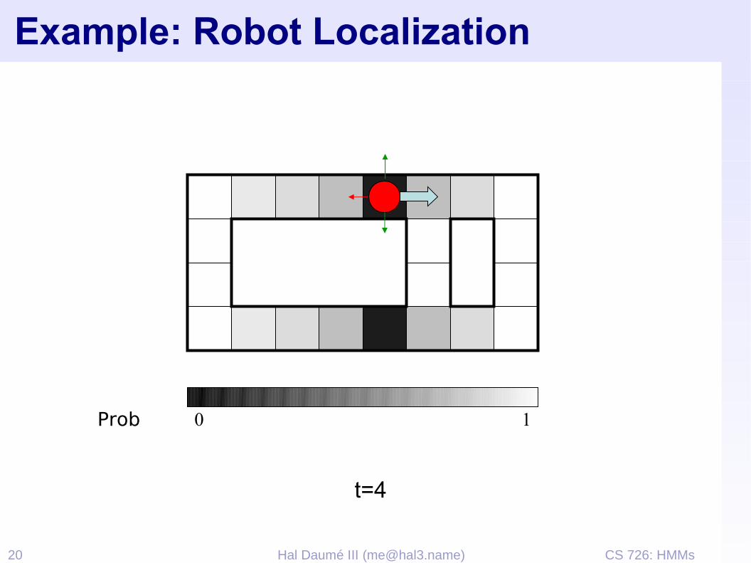
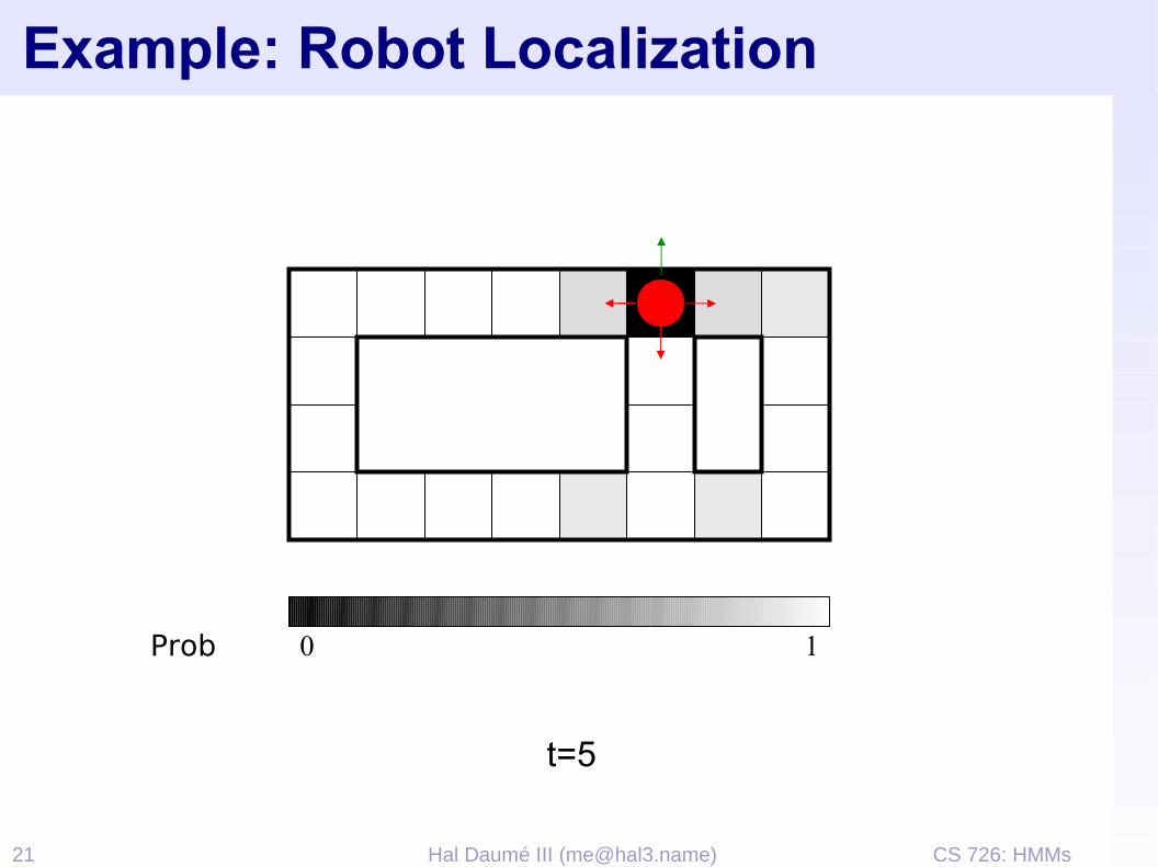
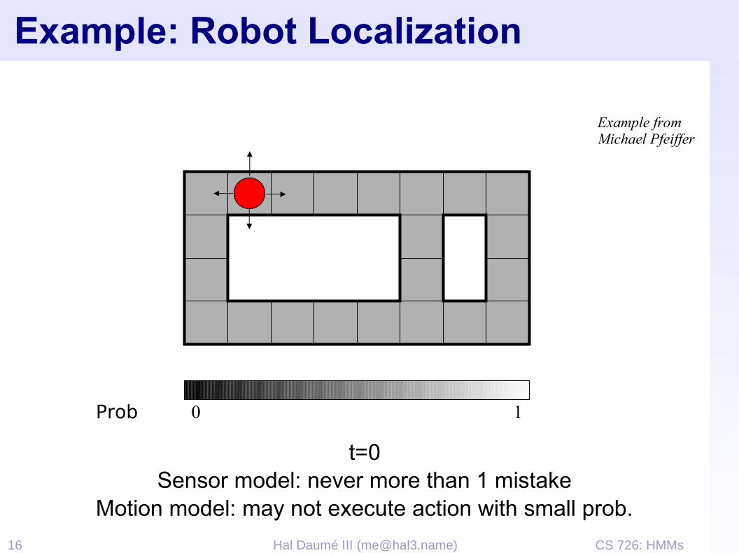
Example: Robot Localization
t=0Sensor model: never more than 1 mistake
Motion model: may not execute action with small prob.
10Prob
Example from Michael Pfeiffer

CS 726: HMMs22 Hal Daumé III ([email protected])
Passage of Time➢ Assume we have current belief P(X | evidence to date)
➢ Then, after one time step passes:
➢ Or, compactly:
➢ Basic idea: beliefs get “pushed” through the transitions➢ With the “B” notation, we have to be careful about what time step t the belief
is about, and what evidence it includes
CS 726: HMMs23 Hal Daumé III ([email protected])
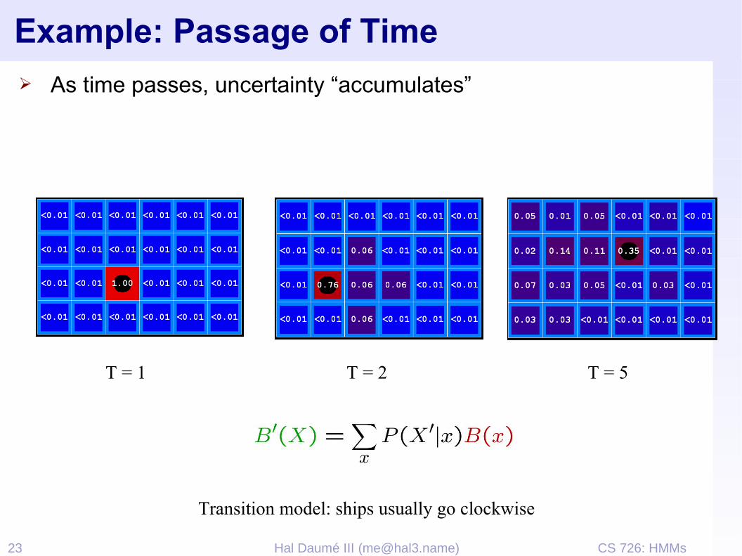
Example: Passage of Time➢ As time passes, uncertainty “accumulates”
T = 1 T = 2 T = 5
Transition model: ships usually go clockwise
CS 726: HMMs24 Hal Daumé III ([email protected])
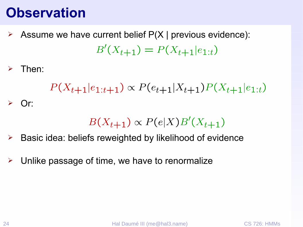
Observation➢ Assume we have current belief P(X | previous evidence):
➢ Then:
➢ Or:
➢ Basic idea: beliefs reweighted by likelihood of evidence
➢ Unlike passage of time, we have to renormalize
CS 726: HMMs25 Hal Daumé III ([email protected])
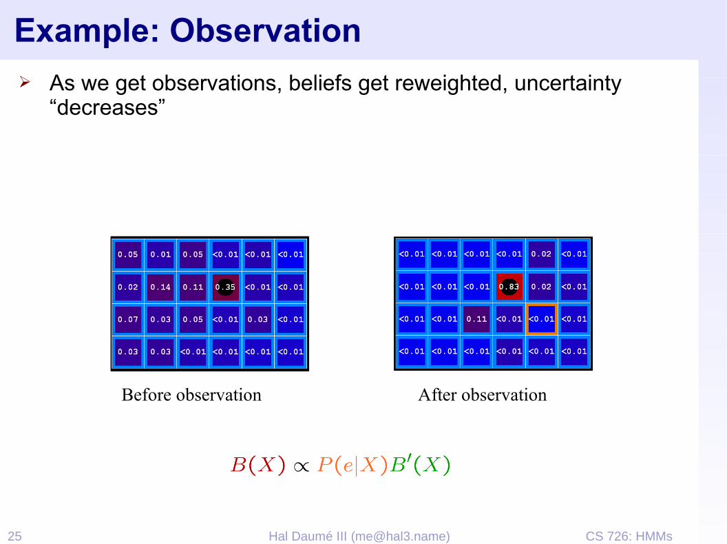
Example: Observation➢ As we get observations, beliefs get reweighted, uncertainty
“decreases”
Before observation After observation

CS 726: HMMs28 Hal Daumé III ([email protected])
Updates: Time Complexity
➢ Every time step, we start with current P(X | evidence)➢ We must update for time:
➢ We must update for observation:
➢ So, linear in time steps, quadratic in number of states |X|➢ Of course, can do both at once, too
CS 726: HMMs29 Hal Daumé III ([email protected])
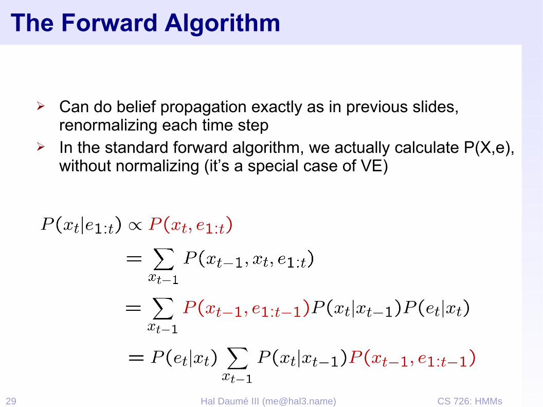
The Forward Algorithm
➢ Can do belief propagation exactly as in previous slides, renormalizing each time step
➢ In the standard forward algorithm, we actually calculate P(X,e), without normalizing (it’s a special case of VE)

CS 726: HMMs30 Hal Daumé III ([email protected])
Particle Filtering➢ Sometimes |X| is too big to use exact inference
➢ |X| may be too big to even store B(X)➢ E.g. X is continuous➢ |X|2 may be too big to do updates
➢ Solution: approximate inference➢ Track samples of X, not all values➢ Time per step is linear in the number of samples➢ But: number needed may be large
➢ This is how robot localization works in practice
0.0 0.1
0.0 0.0
0.0
0.2
0.0 0.2 0.5
CS 726: HMMs31 Hal Daumé III ([email protected])
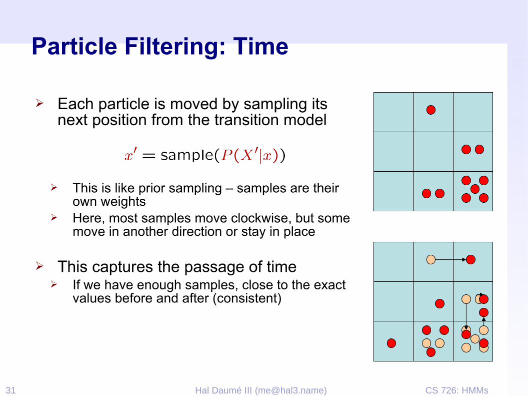
Particle Filtering: Time
➢ Each particle is moved by sampling its next position from the transition model
➢ This is like prior sampling – samples are their own weights
➢ Here, most samples move clockwise, but some move in another direction or stay in place
➢ This captures the passage of time➢ If we have enough samples, close to the exact
values before and after (consistent)

CS 726: HMMs32 Hal Daumé III ([email protected])
Particle Filtering: Observation
➢ Slightly trickier:➢ We don’t sample the observation, we fix it➢ This is similar to likelihood weighting, so
we downweight our samples based on the evidence
➢ Note that, as before, the probabilities don’t sum to one, since most have been downweighted (they sum to an approximation of P(e))
CS 726: HMMs33 Hal Daumé III ([email protected])
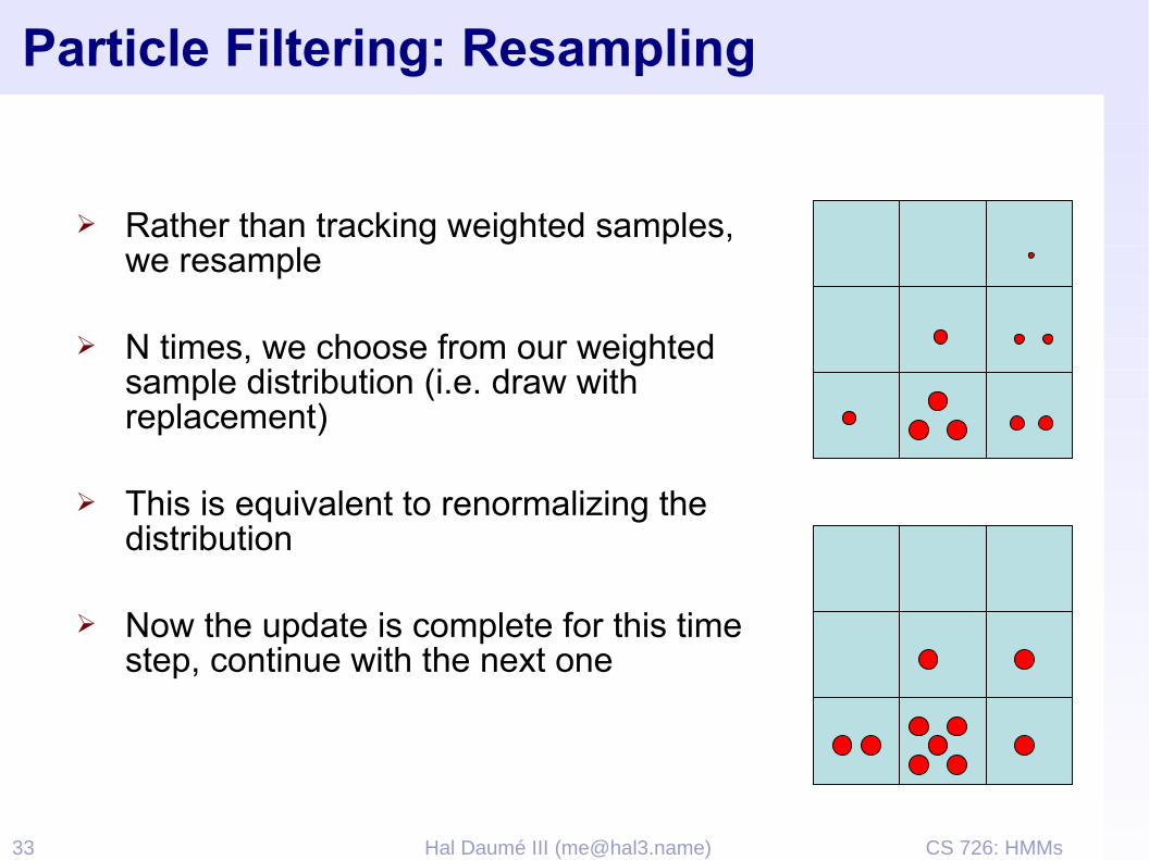
Particle Filtering: Resampling
➢ Rather than tracking weighted samples, we resample
➢ N times, we choose from our weighted sample distribution (i.e. draw with replacement)
➢ This is equivalent to renormalizing the distribution
➢ Now the update is complete for this time step, continue with the next one
CS 726: HMMs34 Hal Daumé III ([email protected])
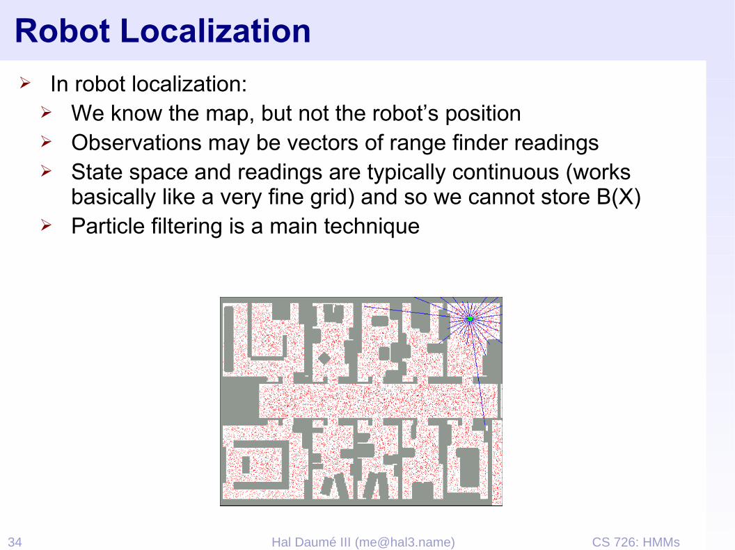
Robot Localization➢ In robot localization:
➢ We know the map, but not the robot’s position➢ Observations may be vectors of range finder readings➢ State space and readings are typically continuous (works
basically like a very fine grid) and so we cannot store B(X)➢ Particle filtering is a main technique
CS 726: HMMs35 Hal Daumé III ([email protected])
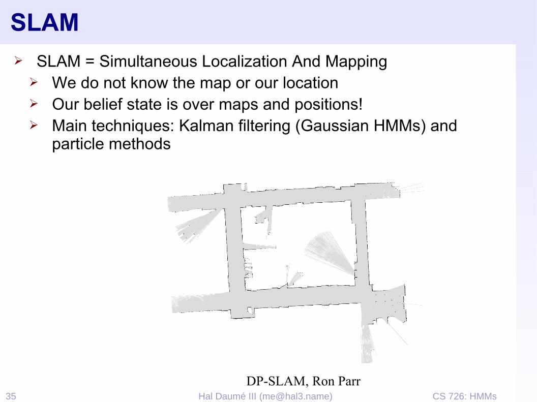
SLAM➢ SLAM = Simultaneous Localization And Mapping
➢ We do not know the map or our location➢ Our belief state is over maps and positions!➢ Main techniques: Kalman filtering (Gaussian HMMs) and
particle methods
DP-SLAM, Ron Parr
CS 726: HMMs36 Hal Daumé III ([email protected])
Most Likely Explanation
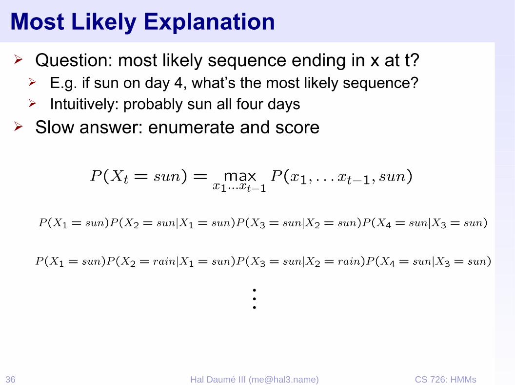
➢ Question: most likely sequence ending in x at t?➢ E.g. if sun on day 4, what’s the most likely sequence?➢ Intuitively: probably sun all four days
➢ Slow answer: enumerate and score
…

CS 726: HMMs37 Hal Daumé III ([email protected])
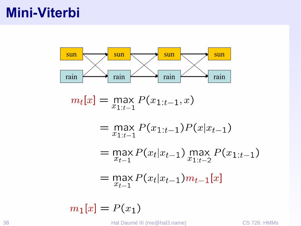
Mini-Viterbi Algorithm
➢ Better answer: cached incremental updates
➢ Define:
➢ Read best sequence off of m and a vectors
sun
rain
sun
rain
sun
rain
sun
rain
CS 726: HMMs39 Hal Daumé III ([email protected])
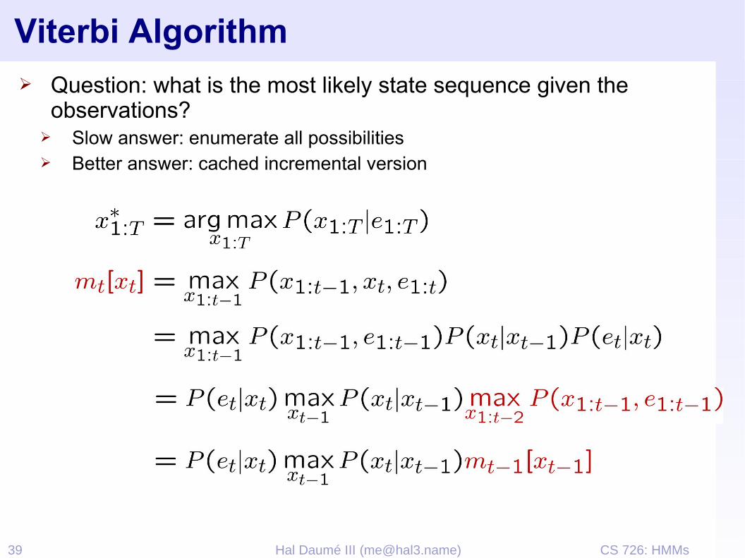
Viterbi Algorithm➢ Question: what is the most likely state sequence given the
observations?➢ Slow answer: enumerate all possibilities➢ Better answer: cached incremental version