he hnisc ec T at ersit Univ au k Chemnitz-Zwic · at ersit Univ au k Chemnitz-Zwic hergrupp orsce...
45
Transcript of he hnisc ec T at ersit Univ au k Chemnitz-Zwic · at ersit Univ au k Chemnitz-Zwic hergrupp orsce...

Technische Universit�at Chemnitz-Zwickau
DFG-Forschergruppe \SPC" � Fakult�at f�ur Mathematik
Werner Rath
Canonical Forms for Linear
Descriptor Systems with Variable
Coe�cients
�
Abstract
We study linear descriptor systems with rectangular variable coe�cient matrices.
Using local and global equivalence transformations we introduce normal and con-
densed forms and get sets of characteristic quantities. These quantities allow us to
decide whether a linear descriptor system with variable coe�cients is regularizable
by derivative and/or proportional state feedback or not. Regularizable by feedback
means for us that their exist a feedback which makes the closed loop system uniquely
solvable for every consistent initial vector.
�
The work has been partially supported under the grant no. Me 790/5-1
\Di�erentiell{algebraische Gleichungen" by the Deutsche Forschungsgemeinschaft.
Preprint-Reihe der Chemnitzer DFG-Forschergruppe
\Scienti�c Parallel Computing"
SPC 95 16 May 1995

Author's addresses:
Werner Rath
Fakult�at f�ur Mathematik
TU Chemnitz{Zwickau
D{09107 Chemnitz
Fed. Rep. Germany
e-mail: [email protected]

1 Introduction
In this paper, we study descriptor systems with linear variable coe�cient
E(t) _x(t) = A(t)x(t) +B(t)u(t) (1)
in the interval [t
1
; t
2
] � R together with an initial condition
x(t
0
) = x
0
: (2)
Let C
r
([t
1
; t
2
]; C
n;l
) denote the set of r-times continuously di�erentiable functions from the
interval [t
1
; t
2
] to the vector space C
n;l
of complex n � l matrices. We assume that
E(t); A(t) 2 C([t
1
; t
2
]; C
n;l
);
B(t) 2 C([t
1
; t
2
]; C
n;m
);
x(t) 2 C([t
1
; t
2
]; C
l
);
u(t) 2 C([t
1
; t
2
]; C
m
)
(3)
and B(t) has full column rank for all t 2 [t
1
; t
2
]. x(t) is called the state and u(t) the control
of the system.
Descriptor systems of the form (1) arise naturally in a variety of circumstances, i.e.
they are used in modelling of mechanical multibody systems [31, 32] and electrical circuits
[19].
The constant coe�cient case shows that one has to have �rst a good understanding of
the behaviour of the corresponding di�erential algebraic equations (DAEs). For a square
constant coe�cient system (n = l)
E _x(t) = Ax(t) +Bu(t) (4)
it is well known that the behaviour of the system (4),(2) (and the corresponding DAE)
depends upon the properties of the matrix pencil
�E � �B: (5)
The system (4) and the corresponding pencil (5) are called regular if
det(�A� �B) 6= 0 for some (�; �) 2 C
2
: (6)
While regularity of the system (4) guarantees the existence and uniqueness of classical
solutions [7, 1], this is not true for the system (1) with variable coe�cients [18, 22].
The constant coe�cient system (4) and the corresponding pencil (5) are said to have
index at most one if the dimension of the largest nilpotent block in the Kronecker canonical
form of the pencil (5) is less than or equal to one (see e.g. [1, 14, 33]). For higher
index descriptor systems (4) impulses can arise if the control is not su�ciently smooth
or the system can even lose causality (see [16, 17, 34]). Therefore, one is interested in a
1

proportional and/or derivative feedback for which the closed loop system is regular and
at most of index one to guarantee existence and uniqueness of the solution and to avoid
impulsive modes [3, 5].
The main di�culty in understanding the DAE that corresponds to the descriptor sys-
tems (1) is that di�erent generalizations of the concepts of solvability, index, etc from
constant DAEs to variable coe�cient DAEs are possible and have been discussed in the
literature [1, 18, 20, 22]. These di�erent concepts can be used as a basis for di�erent results
for linear descriptor systems with variable coe�cients. Until today, only few results have
been achieved in this direction. The results in [11, 12], for example, use the solvability
concepts for DAEs as described in [1, 8, 9, 10].
In a series of articles, Kunkel and Mehrmann discussed a more general solvability con-
cept and presented new canonical forms for linear DAEs with variable coe�cients [22, 24].
Furthermore, they presented new numerical methods based on an index reduction pro-
cess [23]. Recently, Rabier and Rheinboldt generalized this approach [27] and in [29] they
showed that, as in the constant coe�cient case, impulse modes can only occur for higher
index systems.
We will brie y discuss the main results from [22, 24] in Section 2.
In Section 3 and 4 we show that analogous methods can be used to study linear de-
scriptor systems with variable coe�cients. First, we obtain local characteristic quantities
and local canonical forms for the system (1) in Section 3. Then in Section 4, we show that
this local quantities can be used to study the global properties of the system and we end
up with global canonical forms from which we can read o� system properties.
Finally in Section 5 we study under which conditions a linear descriptor system with
variable coe�cients is regularizable. That means we give necessary and su�cient conditions
for the existence of derivative and/or proportional state feedback so that the closed loop
system is uniquely solvable for all consistent initial values. Furthermore Section 5 shows
how we can get in theory a closed loop system of index at most one.
2 Canonical forms for linear di�erential{equations
with variable coe�cients
We begin our analysis of the descriptor system (1), (2) with a short look at canonical forms
for di�erential{algebraic equations (DAEs) with variable coe�cients [22, 24]. These DAEs
are of the form
E(t) _x(t) = A(t)x(t) + f(t); t 2 [t
1
; t
2
] � R (7)
with initial condition (2), E, A as in (3) and f 2 C([t
1
; t
2
]; C
n
).
The standard variable coe�cient transformations that can be applied to linear DAEs
are changes of bases, i.e. x(t) = Q(t)y(t) and pre{multiplication of (7) by P (t). Equation
(7) then transforms to
P (t)E(t)Q(t) _x(t) =
�
P (t)A(t)Q(t)� P (t)E(t)
_
Q(t)
�
x(t) + P (t)x(t) (8)
2

and we get the following de�nition of equivalence for pairs of matrix functions.
De�nition 1 Two pairs of matrix functions (E
i
(t); A
i
(t)); E
i
; A
i
2 C([t
1
; t
2
]; C
n;l
); i = 1; 2
are called equivalent if there are P 2 C([t
1
; t
2
]; C
n;n
) and Q 2 C
1
([t
1
; t
2
]; C
l;l
) with P (t); Q(t)
nonsingular for all t 2 [t
1
; t
2
] such that
(E
2
(t); A
2
(t)) = P (t)(E
1
(t); A
1
(t))
"
Q(t) �
_
Q(t)
0 Q(t)
#
: (9)
This approach is very useful for an analysis of DAEs, but for a numerical solution the
derivative
_
Q(t) creates di�culties. Taking into account that at a �xed point t 2 [t
1
; t
2
]
we can choose Q(t) and
_
Q(t) independently [15, 22] one obtains the following de�nition of
equivalence for constant pencils.
De�nition 2 Two pairs of matrices (E
i
; A
i
); E
i
; A
i
2 C
n;l
; i = 1; 2 are called equivalent
if there are matrices P 2 C
n;n
, Q; R 2 C
l;l
with P;Q nonsingular such that
(E
2
; A
2
) = P (E
1
; A
1
)
"
Q �R
0 Q
#
: (10)
For this local equivalence we �nd in [24] the following canonical form:
Theorem 3 Let E;A 2 C
n;l
and
(a) T basis of kernelE
(b) Z basis of corangeE = kernelE
�
(c) T
0
basis of cokernelE = rangeE
�
(d) V basis of corange(Z
�
AT ):
(11)
Then, the quantities (with the convention rank ; = 0)
(a) r = rankE (rank)
(b) a = rank(Z
�
AT ) (algebraic part)
(c) s = rank(V
�
Z
�
AT
0
) (strangeness)
(d) d = r � s (di�erential part)
(e) u
l
= n� r � a� s (left undetermined part)
(f) u
r
= l � r � a� s (right undetermined part)
(12)
are invariant under (9) and (E;A) is equivalent to the canonical form
0
B
B
B
B
B
B
@
2
6
6
6
6
6
6
4
I
s
0 0 0 0
0 I
d
0 0 0
0 0 0 0 0
0 0 0 0 0
0 0 0 0 0
3
7
7
7
7
7
7
5
;
2
6
6
6
6
6
6
4
0 0 0 0 0
0 0 0 0 0
0 0 I
a
0 0
I
s
0 0 0 0
0 0 0 0 0
3
7
7
7
7
7
7
5
1
C
C
C
C
C
C
A
s
d
a
s
u
(13)
where the last block column in both matrices has width u
r
.
3

Applying now the results for the local canonical form (13) to equation (7) one obtains
functions r; a; s; u
l
; u
r
: [t
1
; t
2
] ! N
0
. Currently we do not know in general how to char-
acterize points, where these quantities change their values with t. For these reasons, we
exclude such phenomena by assuming
r(t) � r; a(t) � a; s(t) � s; u
l
(t) � u
l
; u
r
(t) � u
r
: (14)
For analytic matrix functions E(t); A(t) the functions r(t); a(t); s(t); u
l
(t); u
r
(t) change
their values only at isolated points and for the theory such points do not cause any
problems.
1
For nonanalytic matrix functions E(t); A(t) a characterization of such points is
still under investigation. Recently, Rabier and Rheinboldt [28, 29] generalized the approach
of [22, 24] and studied generalized (weak) solutions of the DAE (7).
Applying equivalence (9) to the pair (E(t); A(t)) we obtain from [24] the following
canonical form:
Theorem 4 Let E;A as in (3) and let (14) hold. Then (E(t); A(t)) is equivalent to a pair
of matrix functions of the form
0
B
B
B
B
B
B
@
2
6
6
6
6
6
6
4
I
s
0 0 0 0
0 I
d
0 0 0
0 0 0 0 0
0 0 0 0 0
0 0 0 0 0
3
7
7
7
7
7
7
5
;
2
6
6
6
6
6
6
4
0 A
12
(t) 0 A
14
(t) A
15
(t)
0 0 0 A
24
(t) A
25
(t)
0 0 I
a
0 0
I
s
0 0 0 0
0 0 0 0 0
3
7
7
7
7
7
7
5
1
C
C
C
C
C
C
A
s
d
a
s
u
l
(15)
where the last block column in both matrices has width u
r
.
Writing down the system of di�erential{algebraic equations that corresponds to (15),
we get
(a) _x
1
(t) = A
12
(t)x
2
(t) +A
14
(t)x
4
(t) +A
15
(t)x
5
(t) + f
1
(t)
(b) _x
2
(t) = A
24
(t)x
4
(t) +A
25
(t)x
5
(t) + f
2
(t)
(c) 0 = x
3
(t) + f
3
(t)
(d) 0 = x
1
(t) + f
4
(t)
(e) 0 = f
5
(t):
(16)
Now we can di�erentiate equation (16d) and insert it in (16a). This corresponds to passing
from (15) to
0
B
B
B
B
B
B
@
2
6
6
6
6
6
6
4
0 0 0 0 0
0 I
d
0 0 0
0 0 0 0 0
0 0 0 0 0
0 0 0 0 0
3
7
7
7
7
7
7
5
;
2
6
6
6
6
6
6
4
0 A
12
(t) 0 A
14
(t) A
15
(t)
0 0 0 A
24
(t) A
25
(t)
0 0 I
a
0 0
I
s
0 0 0 0
0 0 0 0 0
3
7
7
7
7
7
7
5
1
C
C
C
C
C
C
A
s
d
a
s
u
l
(17)
1
For analytic E(t); A(t) we can use the analytic singular value decomposition [2, 26, 35] to compute a
cononical form similar to (15) where we get �(t)'s instead of the identities. These �(t)'s are diagonal and
can become singular only at isolated points.
4

for which we again compute characteristic values r; a; s; d; u
l
; u
r
.
The above procedure leads to an inductive de�nition of a sequence of pairs of matrix
functions (E
i
(t); A
i
(t)); i 2 N
0
, where (E
0
(t); A
0
(t)) = (E(t); A(t)) and (E
i+1
(t); A
i+1
(t))
is derived from (E
i
(t); A
i
(t)) by one step of this procedure.
Here we must assume (14) for every occurring pair of matrices. Connected with this
sequence, we then have sequences r
i
; a
i
; s
i
; d
i
; u
l
i
; u
r
i
; i 2 N
0
of nonnegative integers. The
sequences r
i
; a
i
; s
i
; i 2 N
0
are characteristic for the given DAE, that is, they do not depend
on the speci�c way they are obtained (recall that d
i
; u
l
i
; u
r
i
are not independent of these).
Furthermore, the sequences stop after �nitely many (say �) steps with s
i
= 0. The quantity
� is called the strangeness index of the pencil (E(t); A(t)).
As last result from [22, 24] we cite an appropriate generalization of the Weierstra�{
Kronecker canonical form for constant pencils (E;A) in the case of variable pencils:
Theorem 5 Let the strangeness index � be well-de�ned for the pair (E(t); A(t)) of smooth
matrix functions. Let r
i
; a
i
; s
i
; d
i
; u
l
i
; u
r
i
; i 2 N
0
be the related characteristic values as above.
De�ne
(a) b
0
= a
0
; b
i
= rank
�h
A
(i�1)
14
(t) A
(i�1)
15
(t)
i�
;
(b) c
0
= a
0
+ s
0
; c
i
= rank
�h
A
(i�1)
12
(t) A
(i�1)
14
(t) A
(i�1)
15
(t)
i�
;
(c) w
0
= u
l
0
; w
i
= u
l
i
� u
l
i�1
; i = 1; : : : ; �:
(18)
We then have
(a) c
i
= b
i
+ s
i
; i = 0; : : : ; �
(b) w
i
= s
i�1
� c
i
; i = 1; : : : ; �
(19)
and the pair (E(t); A(t)) is equivalent to a pair of matrix functions of the form (without
arguments)
0
B
B
B
B
B
B
B
B
B
B
B
B
B
B
B
B
B
B
B
@
2
6
6
6
6
6
6
6
6
6
6
6
6
6
6
6
6
6
6
6
4
I 0 : : : 0 0 � : : : �
0 0 : : : 0 0 F
m
�
.
.
.
.
.
.
.
.
.
.
.
.
.
.
.
.
.
.
.
.
.
.
.
.
.
.
.
F
1
0 0 : : : 0 0
0 0 : : : 0 0 G
m
�
.
.
.
.
.
.
.
.
.
.
.
.
.
.
.
.
.
.
.
.
.
.
.
.
.
.
.
G
1
0 0 : : : 0 0
3
7
7
7
7
7
7
7
7
7
7
7
7
7
7
7
7
7
7
7
5
;
2
6
6
6
6
6
6
6
6
6
6
6
6
6
6
6
6
6
6
6
4
� � : : : � 0 : : : : : : 0
0 0 : : : 0 0 : : : : : : 0
.
.
.
.
.
.
.
.
.
.
.
.
.
.
.
.
.
.
.
.
.
.
.
.
.
.
.
.
.
.
0 0 : : : 0 0 : : : : : : 0
0 0 : : : 0 I
.
.
.
.
.
.
.
.
.
.
.
.
.
.
.
.
.
.
.
.
.
.
.
.
0 0 : : : 0 I
3
7
7
7
7
7
7
7
7
7
7
7
7
7
7
7
7
7
7
7
5
1
C
C
C
C
C
C
C
C
C
C
C
C
C
C
C
C
C
C
C
A
d
�
w
�
.
.
.
.
.
.
w
0
c
�
.
.
.
.
.
.
c
0
(20)
where
rank
"
F
i
G
i
#!
= c
i
+ w
i
= s
i�1
� c
i�1
(21)
and the second block column in both matrices has width u
r
�
.
5

In the next two sections we will prove generalizations of these theorems for the descriptor
system (1).
3 Local canonical forms
In this section we will generalize the local canonical form for linear DAEs with variable
coe�cients of Theorem 3 for the descriptor system (1).
For constant coe�cient systems canonical and condensed forms have been studied for
unitary transformations in [3, 4, 5] and for general transformations in [25].
Note that for a linear descriptor system with variable coe�cients (1) we cannot apply
directly the results of Section 2 since usually we cannot assume that the control u(t) is
su�ciently di�erentiable. In principle we can apply di�erentiation of components only in
the uncontrollable subspace, i.e., the part of the system operating in the left nullspace of
B(t). Recently, a condensed form for unitary transformations has been studied in [6]. In
the approach of [11, 12] it is assumed that the control is su�ciently smooth, which is a
major di�erence to our approach.
The standard variable coe�cient transformations that can be applied to the linear de-
scriptor system (1) are pre{multiplication of (1) by a nonsingular matrix P (t) and changes
of the bases for the state x(t) and control u(t) of the system. Therefore, we use the following
global equivalence transformations for a triple of matrix functions (E(t); A(t); B(t)).
De�nition 6 Two triples of matrix functions (E
i
(t); A
i
(t); B
i
(t)), B
i
(t) 2 C([t
1
; t
2
]; C
n;m
),
E
i
(t); A
i
(t) 2 C([t
1
; t
2
]; C
n;l
),i = 1; 2 are called equivalent if there are P (t) 2 C([t
1
; t
2
]; C
n;n
),
Q(t) 2 C([t
1
; t
2
]; C
l;l
) and S(t) 2 C([t
1
; t
2
]; C
m;m
) with P (t); Q(t); S(t) nonsingular for all
t 2 [t
1
; t
2
] such that
(E
2
(t); A
2
(t); B
2
(t)) = P (t)(E
1
(t); A
1
(t); B
1
(t))
2
6
4
Q(t) �
_
Q(t) 0
0 Q(t) 0
0 0 S(t)
3
7
5
: (22)
Standard rules for di�erentiation show that this is indeed an equivalence relation.
As in the case of linear DAEs we get the responding local equivalence by choosing
_
Q(t)
independent of Q(t) at a �xed point t 2 [t
1
; t
2
].
De�nition 7 Two triples of matrices (E
i
; A
i
; B
i
); E
i
; A
i
2 C
n;l
; B
i
2 C
n;m
; i = 1; 2
are called equivalent if there are matrices P 2 C
n;n
, Q;R 2 C
l;l
, S 2 C
m;m
with P;Q; S
nonsingular such that
(E
2
; A
2
; B
2
) = P (E
1
; A
1
; B
1
)
2
6
4
Q �R 0
0 Q 0
0 0 S
3
7
5
: (23)
6

Again, it is easily checked that the local transformations describe an equivalence trans-
formation.
Using the local equivalence transformations we obtain the following canonical form for
a triple of matrices (E;A;B).
Theorem 8 Let E;A 2 C
n;l
; B 2 C
n;m
and
(a) T basis of kernelE
(b) Z basis of corangeE = kernelE
�
(c) T
0
basis of cokernelE = rangeE
�
(d) K basis of corange(Z
�
B)
(e) V basis of corange(K
�
Z
�
AT )
(f) L basis of kernel(Z
�
B)
(g) Y basis of kernel(V
�
K
�
Z
�
AT
0
)
(h) Y
0
basis of cokernel(V
�
K
�
Z
�
AT
0
)
(i) N basis of kernel([I
s
0][Y
0
Y ]
�1
(Z
0�
ET
0
)
�1
Z
0�
BL):
(24)
Then, the quantities
(a) r = rankE (rank)
(b) f = rank(Z
�
B) (feedback part)
(c) a = rank(K
�
Z
�
AT ) (algebraic part)
(d) s = rank(V
�
K
�
Z
�
AT
0
) (strangeness)
(e) d = r � s (di�erential part)
(f) u
l
= n� r � a� s� f (left undetermined part)
(g) u
r
= l� r � a� s (right undetermined part)
(h) v = m� f
(i) s
c
= rank([I
s
0][Y
0
Y ]
�1
(Z
0�
ET
0
)
�1
Z
0�
BL
(j) s
u
= s� s
c
(k) d
c
= rank([0 I
d
][Y
0
Y ]
�1
(Z
0�
ET
0
)
�1
Z
0�
BLN
(l) d
u
= d� d
c
:
(25)
7

are invariant under (23) and (E;A;B) is equivalent to the canonical form
0
B
B
B
B
B
B
B
B
B
B
B
B
B
B
B
@
2
6
6
6
6
6
6
6
6
6
6
6
6
6
6
6
4
I
s
c
0 0 0 0 0 0 0
0 I
s
u
0 0 0 0 0 0
0 0 I
d
c
0 0 0 0 0
0 0 0 I
d
u
0 0 0 0
0 0 0 0 0 0 0 0
0 0 0 0 0 0 0 0
0 0 0 0 0 0 0 0
0 0 0 0 0 0 0 0
0 0 0 0 0 0 0 0
3
7
7
7
7
7
7
7
7
7
7
7
7
7
7
7
5
;
2
6
6
6
6
6
6
6
6
6
6
6
6
6
6
6
4
0 0 0 0 0 0 0 0
0 0 0 0 0 0 0 0
0 0 0 0 0 0 0 0
0 0 0 0 0 0 0 0
0 0 0 0 I
a
0 0 0
I
s
c
0 0 0 0 0 0 0
0 I
s
u
0 0 0 0 0 0
0 0 � � 0 � � �
0 0 0 0 0 0 0 0
3
7
7
7
7
7
7
7
7
7
7
7
7
7
7
7
5
;
2
6
6
6
6
6
6
6
6
6
6
6
6
6
6
6
4
0 I
s
c
0
0 0 0
0 0 I
d
c
0 0 0
0 0 0
0 0 0
0 0 0
I
f
0 0
0 0 0
3
7
7
7
7
7
7
7
7
7
7
7
7
7
7
7
5
1
C
C
C
C
C
C
C
C
C
C
C
C
C
C
C
A
s
c
s
u
d
c
d
u
a
s
c
s
u
f
u
l
:
(26)
and the last column in the �rst and second matrix has width u
r
.
Proof. Let (E
i
; A
i
; B
i
); i = 1; 2, be equivalent. Since
rank(E
2
) = rank(PE
1
Q) = rank(E
1
);
r is invariant. For f; a; s; s
c
and d
c
we must �rst show that they are well{de�ned with
respect to the choice of the bases. Each change of bases can be represented by
~
T = TM
T
;
~
Z = ZM
Z
;
~
T
0
= T
0
M
T
0
;
~
Z
0
= Z
0
M
Z
0
;
~
K =M
�1
Z
KM
K
;
~
V =M
�1
K
VM
V
~
L = LM
L
;
~
Y
0
=M
�1
T
0
Y
0
M
Y
0
;
~
Y =M
�1
T
0
YM
Y
;
~
N =M
�1
L
NM
N
with nonsingular matrices M
T
; M
Z
; M
T
0
; M
K
; M
V
; M
L
; M
Y
0
; M
Y
and M
N
. The well{
de�niteness follows from
rank(
~
Z
�
B) = rank(M
�
Z
Z
�
B) = rank(Z
�
B);
rank
�
[I
s
0][
~
Y
0
~
Y ]
�1
(
~
Z
0
�
E
~
T
0
)
�1
~
Z
0
�
B
~
L
�
= rank
�
[I
s
0][M
�1
T
0
Y
0
M
Y
0
M
�1
T
0
YM
Y
]
�1
� (M
�
Z
0
Z
0�
ET
0
M
T
0
)
�1
M
�
Z
0
Z
0�
BLM
L
�
8

= rank
�
[I
s
0]
�
diag(M
�1
Y
0
M
�1
Y
)[Y
0
Y ]
�1
M
T
0
�
�
�
M
�1
T
0
(Z
0�
ET
0
)
�1
M
��
Z
0
�
M
�
Z
0
Z
0�
BLM
L
�
= rank
�
M
�1
Y
0
[I
s
0][Y
0
Y ]
�1
(Z
0�
ET
0
)
�1
Z
0�
BLM
L
�
= rank
�
[I
s
0][Y
0
Y ]
�1
(Z
0�
ET
0
)
�1
Z
0�
BL
�
and similar calculations for the other values.
Let now bases T
2
; Z
2
; Z
0
2
; T
0
2
;K
2
; V
2
; L
2
; Y
0
2
; Y
2
; N
2
be given for (E
2
; A
2
; B
2
), i.e.
rank(E
2
T
2
) = 0; T
�
2
T
2
nonsingular; rank(T
�
2
T
2
) = n � r
rank(Z
�
2
E
2
) = 0; Z
�
2
Z
2
nonsingular; rank(Z
�
2
Z
2
) = n� r
rank(E
2
T
0
2
) = r; T
0
�
2
T
0
2
nonsingular; rank(T
0�
2
T
0
2
) = r
rank(Z
0
2
�
E
2
) = r; Z
0
2
�
Z
0
2
nonsingular; rank(Z
0�
2
Z
0
2
) = r
rank(K
2
Z
�
2
B
2
) = 0; K
�
2
K
2
nonsingular; rank(K
�
2
K
2
) =
^
f
2
rank(V
�
2
Z
�
2
K
�
2
A
2
T
2
) = 0; V
�
2
V
2
nonsingular; rank(V
�
2
V
2
) = a
2
rank(Z
�
2
B
2
L
2
) = 0; L
�
2
L
2
nonsingular; rank(K
�
2
K
2
) = f
2
rank(V
�
2
Z
�
2
A
2
T
0
2
Y
2
) = 0; Y
�
2
Y
2
nonsingular; rank(Y
�
2
Y
2
) = s
2
rank(V
�
2
Z
�
2
A
2
T
0
2
Y
0
2
) = s
2
; Y
0
�
2
Y
0
2
nonsingular; rank(Y
0
2
�
Y
0
2
) = s
2
rank([I
s
0][Y
0
2
Y
2
]
�1
(Z
0
2
�
E
2
T
0
2
)
�1
Z
0
2
�
B
2
L
2
N
2
) = d
c
2
;
N
�
2
N
2
nonsingular; rank(N
�
2
N
2
) = d
c
2
with
^
f
2
= dim(corange(Z
�
2
B
2
)), a
2
= dim(corange(Z
�
2
K
�
2
A
2
T
2
)) and s
2
=
dim(kernel(V
�
2
Z
�
2
A
2
T
0
2
)). Using (23) and setting
T
1
= QT
2
; Z
�
1
= Z
�
2
P; T
0
1
= QT
0
2
; Z
0
1
�
= Z
0
2
�
P; K
�
1
= K
�
2
; V
�
1
= V
�
2
L
1
=WL
2
; Y
1
= Y
2
; Y
0
1
= Y
0
2
; N
1
= N
2
we obtain the same relations for (E
1
; A
1
; B
1
) and the above T
1
; Z
1
; T
0
1
;K
1
; V
1
; L
1
; Y
1
; Y
0
1
; N
1
,
i.e. they form bases according to (24). Since
f
2
= rank(Z
�
2
B
2
)
= rank(Z
�
2
PB
1
W )
= rank(Z
�
1
B
1
) = f
1
we get the invariance of f . With the same technique, the invariance of a and s can be
shown. s
c
is invariant, since
s
c
2
= rank([I
s
0][Y
0
2
Y
2
]
�1
(Z
0
2
�
E
2
T
0
2
)
�1
Z
0
2
�
B
2
L
2
)
= rank([I
s
0][Y
0
1
Y
1
]
�1
(Z
0
2
�
PE
1
QT
0
2
)
�1
Z
0
2
�
PB
1
WL
2
)
= rank([I
s
0][Y
0
1
Y
1
]
�1
(Z
0
1
�
E
1
T
0
1
)
�1
Z
0
1
�
B
1
L
1
) = s
c
1
;
this also holds for N
1
, i.e. d
c
is invariant. Therefore, the invariance of the other values in
(25) follows immediately.
9

For the derivation of the canonical form (26) we always use nonsingular transformation
matrices, i.e. in the �rst step we take a basis Z
0
of rangeE and set Q = [Z
0
Z], etc. As
result we obtain the following sequence of equivalent (�) matrix pairs:
(E;A;B) �
"
Z
0
�
ET
0
0
0 0
#
;
"
Z
0
�
AT
0
Z
0
�
AT
Z
�
AT
0
Z
�
AT
#
;
"
Z
0
�
B
Z
�
B
# !
�
0
B
@
2
6
4
Z
0
�
ET
0
0
0 0
0 0
3
7
5
;
2
6
4
� �
K
0
�
Z
�
AT
0
K
0
�
Z
�
AT
K
�
Z
�
AT
0
K
�
Z
�
AT
3
7
5
;
2
6
4
Z
0
�
BL
0
Z
0
�
BL
K
0
�
Z
�
BL
0
0
0 0
3
7
5
1
C
A
�
0
B
@
2
6
4
I
r
0
0 0
0 0
3
7
5
;
2
6
4
� �
K
0
�
Z
�
AT
0
K
0
�
Z
�
AT
K
�
Z
�
AT
0
K
�
Z
�
AT
3
7
5
;
2
6
4
(Z
0
�
ET
0
)
�1
Z
0
�
BL
0
(Z
0
�
ET
0
)
�1
Z
0
�
BL
K
0
�
Z
�
BL
0
0
0 0
3
7
5
1
C
A
�
0
B
@
2
6
4
I
r
0
0 0
0 0
3
7
5
;
2
6
4
� �
K
0
�
Z
�
AT
0
K
0
�
Z
�
AT
K
�
Z
�
AT
0
K
�
Z
�
AT
3
7
5
;
2
6
4
0 (Z
0
�
ET
0
)
�1
Z
0
�
BL
I
f
0
0 0
3
7
5
1
C
A
�
0
B
@
2
6
4
I
r
0
0 0
0 0
3
7
5
;
2
6
4
0 0
K
0
�
Z
�
AT
0
K
0
�
Z
�
AT
K
�
Z
�
AT
0
K
�
Z
�
AT
3
7
5
;
2
6
4
0 (Z
0
�
ET
0
)
�1
Z
0
�
BL
I
f
0
0 0
3
7
5
1
C
A
�
0
B
B
B
@
2
6
6
6
4
I
r
0 0
0 0 0
0 0 0
0 0 0
3
7
7
7
5
;
2
6
6
6
4
0 0 0
� � �
V
0
�
K
�
Z
�
AT
0
I
a
0
V
�
K
�
Z
�
AT
0
0 0
3
7
7
7
5
;
2
6
6
6
4
0 (Z
0
�
ET
0
)
�1
Z
0
�
BL
I
f
0
0 0
0 0
3
7
7
7
5
1
C
C
C
A
�
0
B
B
B
@
2
6
6
6
4
I
r
0 0
0 0 0
0 0 0
0 0 0
3
7
7
7
5
;
2
6
6
6
4
0 0 0
� � �
0 I
a
0
V
�
K
�
Z
�
AT
0
0 0
3
7
7
7
5
;
2
6
6
6
4
0 (Z
0
�
ET
0
)
�1
Z
0
�
BL
I
f
0
0 0
0 0
3
7
7
7
5
1
C
C
C
A
�
0
B
B
B
@
2
6
6
6
4
I
r
0 0
0 0 0
0 0 0
0 0 0
3
7
7
7
5
;
2
6
6
6
4
0 0 0
� 0 �
0 I
a
0
V
�
K
�
Z
�
AT
0
0 0
3
7
7
7
5
;
2
6
6
6
4
0 (Z
0
�
ET
0
)
�1
Z
0
�
BL
I
f
0
0 0
0 0
3
7
7
7
5
1
C
C
C
A
�
0
B
B
B
B
B
B
B
B
@
2
6
6
6
6
6
6
6
6
4
I
s
0 0 0 0
0 I
d
0 0 0
0 0 0 0 0
0 0 0 0 0
0 0 0 0 0
0 0 0 0 0
3
7
7
7
7
7
7
7
7
5
;
2
6
6
6
6
6
6
6
6
4
0 0 0 0 0
0 0 0 0 0
� � 0 � �
0 0 I
a
0 0
I
s
0 0 0 0
0 0 0 0 0
3
7
7
7
7
7
7
7
7
5
;
2
6
6
6
6
6
6
6
6
4
0 B
12
0 B
22
I
f
0
0 0
0 0
0 0
3
7
7
7
7
7
7
7
7
5
1
C
C
C
C
C
C
C
C
A
10

where B
12
= [I
s
0][Y
0
Y ]
�1
(Z
0
�
ET
0
)
�1
Z
0
�
BL and
B
22
= [0 I
d
][Y
0
Y ]
�1
(Z
0
�
ET
0
)
�1
Z
0
�
BL
�
0
B
B
B
B
B
B
B
B
@
2
6
6
6
6
6
6
6
6
4
I
s
0 0 0 0
0 I
d
0 0 0
0 0 0 0 0
0 0 0 0 0
0 0 0 0 0
0 0 0 0 0
3
7
7
7
7
7
7
7
7
5
;
2
6
6
6
6
6
6
6
6
4
0 0 0 0 0
0 0 0 0 0
0 0 I
a
0 0
I
s
0 0 0 0
0 � 0 � �
0 0 0 0 0
3
7
7
7
7
7
7
7
7
5
;
2
6
6
6
6
6
6
6
6
4
0 B
12
0 B
22
0 0
0 0
I
f
0
0 0
3
7
7
7
7
7
7
7
7
5
1
C
C
C
C
C
C
C
C
A
�
0
B
B
B
B
B
B
B
B
B
B
B
B
B
@
2
6
6
6
6
6
6
6
6
6
6
6
6
6
4
I
s
c
0 0 0 0 0 0
0 I
s
u
0 0 0 0 0
0 0 I
d
0 0 0 0
0 0 0 0 0 0 0
0 0 0 0 0 0 0
0 0 0 0 0 0 0
0 0 0 0 0 0 0
0 0 0 0 0 0 0
3
7
7
7
7
7
7
7
7
7
7
7
7
7
5
;
2
6
6
6
6
6
6
6
6
6
6
6
6
6
4
0 0 0 0 0 0 0
0 0 0 0 0 0 0
0 0 0 0 0 0 0
0 0 0 I
a
0 0 0
I
s
c
0 0 0 0 0 0
0 I
s
u
0 0 0 0 0
0 0 � 0 � � �
0 0 0 0 0 0 0
3
7
7
7
7
7
7
7
7
7
7
7
7
7
5
;
2
6
6
6
6
6
6
6
6
6
6
6
6
6
4
0 I
s
c
0
0 0 0
0 0 [0 I
d
](Z
0
�
ET
0
)
�1
Z
0
�
BLN
0 0 0
0 0 0
0 0 0
I
f
0 0
0 0 0
3
7
7
7
7
7
7
7
7
7
7
7
7
7
5
1
C
C
C
C
C
C
C
C
C
C
C
C
C
A
;
which at last leads to (26) by a similar �nal transformation step.
If we do not split the d and s blocks of B(t) in the proof of Theorem 8 we get the
following condensed form.
Corollary 9 Let E;A 2 C
n;l
; B 2 C
n;m
.Then (E;A;B) is equivalent to the form
0
B
B
B
B
B
B
B
B
@
2
6
6
6
6
6
6
6
6
4
I
s
0 0 0 0
0 I
d
0 0 0
0 0 0 0 0
0 0 0 0 0
0 0 0 0 0
0 0 0 0 0
3
7
7
7
7
7
7
7
7
5
;
2
6
6
6
6
6
6
6
6
4
0 0 0 0 0
0 0 0 0 0
0 0 I
a
0 0
I
s
0 0 0 0
0 � 0 � �
0 0 0 0 0
3
7
7
7
7
7
7
7
7
5
;
2
6
6
6
6
6
6
6
6
4
0 �
0 �
0 0
0 0
I
f
0
0 0
3
7
7
7
7
7
7
7
7
5
1
C
C
C
C
C
C
C
C
A
s
d
a
s
f
u
l
: (27)
where the last block column in the �rst and second matrix has width u
r
and the last block
column of the last matrix has width v. The quantities s; d; a; f; u
l
; u
r
and v are de�ned as
in Theorem 8 and invariant under (23).
11

4 Global canonical forms
As in Section 2, we can apply the results for the local canonical form (26) to equation (1)
and one obtains functions r; f; a; s; s
c
; d
c
: [t
1
; t
2
]! N
0
. Note that the other values depend
only on this invariants. Again, we do not know in general how to characterise points,
where these quantities change their values with t. Therefore, we exclude such phenomena
by assuming
r(t) � r; f(t) � f; a(t) � a; s(t) � s; s
c
(t) � s
c
; d
c
(t) � d
c
: (28)
Applying transformation (22) to (1) we get the following canonical form:
Theorem 10 Let E;A;B in (1) be su�ciently smooth and let (28) hold. Then the triple
(E(t); A(t); B(t)) is equivalent to a triple of matrix functions of the form
0
B
B
B
B
B
B
B
B
B
B
B
B
B
B
@
2
6
6
6
6
6
6
6
6
6
6
6
6
6
6
4
I
s
c
0 0 0 0 0 0 0
0 I
s
u
0 0 0 0 0 0
0 0 I
d
c
0 0 0 0 0
0 0 0 I
d
u
0 0 0 0
0 0 0 0 0 0 0 0
0 0 0 0 0 0 0 0
0 0 0 0 0 0 0 0
0 0 0 0 0 0 0 0
0 0 0 0 0 0 0 0
3
7
7
7
7
7
7
7
7
7
7
7
7
7
7
5
;
2
6
6
6
6
6
6
6
6
6
6
6
6
6
6
4
0 0 A
13
(t) A
14
(t) 0 A
16
(t) A
17
(t) A
18
(t)
0 0 A
23
(t) A
24
(t) 0 A
26
(t) A
27
(t) A
28
(t)
0 0 0 A
34
(t) 0 A
36
(t) A
37
(t) A
38
(t)
0 0 A
43
(t) 0 0 A
46
(t) A
47
(t) A
48
(t)
0 0 0 0 I
a
0 0 0
I
s
c
0 0 0 0 0 0 0
0 I
s
u
0 0 0 0 0 0
0 0 A
83
(t) A
84
(t) 0 A
86
(t) A
87
(t) A
88
(t)
0 0 0 0 0 0 0 0
3
7
7
7
7
7
7
7
7
7
7
7
7
7
7
5
;
2
6
6
6
6
6
6
6
6
6
6
6
6
6
6
4
0 I
s
c
0
0 0 0
0 0 I
d
c
0 0 0
0 0 0
0 0 0
0 0 0
I
f
0 0
0 0 0
3
7
7
7
7
7
7
7
7
7
7
7
7
7
7
5
1
C
C
C
C
C
C
C
C
C
C
C
C
C
C
A
s
c
s
u
d
c
d
u
a
s
c
s
u
f
u
l
:
(29)
The proof of Theorem 10 is given in Appendix A.
Again, as in Section 3 we get a condensed form if we do not split the d and s blocks of
B(t).
Corollary 11 Let E;A;B in (1) be su�ciently smooth and let
r(t) � r; f(t) � f; a(t) � a; s(t) � s
12

hold. Then (E(t); A(t); B(t)) is equivalent to a triple of matrix functions of the form
0
B
B
B
B
B
B
B
B
@
2
6
6
6
6
6
6
6
6
4
I
s
0 0 0 0
0 I
d
0 0 0
0 0 0 0 0
0 0 0 0 0
0 0 0 0 0
0 0 0 0 0
3
7
7
7
7
7
7
7
7
5
;
2
6
6
6
6
6
6
6
6
4
0 A
12
(t) 0 A
14
(t) A
15
(t)
0 0 0 A
24
(t) A
25
(t)
0 0 I
a
0 0
I
s
0 0 0 0
0 A
52
(t) 0 A
54
(t) A
55
(t)
0 0 0 0 0
3
7
7
7
7
7
7
7
7
5
;
2
6
6
6
6
6
6
6
6
4
0 B
12
(t)
0 B
22
(t)
0 0
0 0
I
f
0
0 0
3
7
7
7
7
7
7
7
7
5
1
C
C
C
C
C
C
C
C
A
s
d
a
s
f
u
l
: (30)
From the analysis of linear DAEs with variable coe�cients we know that higher index
problems, i.e., of the index greater than one, are indicated by a non{vanishing strangeness
s (see [24]).
Our main goal is, to study the regularization of the descriptor system (1) by feedback.
As the next lemma shows, Corollary 11 is a �rst step in this direction.
Lemma 12 Let a quadratic descriptor system (1), i.e. n = l, be in the form (30) and
assume that s = 0.
If u
l
= 0, then their exists a state feedback u(t) = F (t)x(t)+ w(t), such that the closed
loop system
E(t) _x(t) = (A(t) +B(t)F (t))x(t)+B(t)w(t); x(t
0
) = x
0
is uniquely solvable for every consistent initial value x
0
and any given control w(t).
Proof. The descriptor system is of the form
2
6
4
I
d
0 0
0 0 0
0 0 0
3
7
5
_x(t) =
2
6
4
0 0 A
13
(t)
0 I
a
0
A
31
(t) 0 A
33
(t)
3
7
5
x(t) +
2
6
4
0 B
12
(t)
0 0
I
f
0
3
7
5
w(t):
Choosing F (t) =
"
�A
31
(t) 0 I
f
�A
33
(t)
0 0 0
#
, we get the closed loop system
2
6
4
I
d
0 0
0 0 0
0 0 0
3
7
5
_x(t) =
2
6
4
0 0 A
13
(t)
0 I
a
0
0 0 I
f
3
7
5
x(t) +
2
6
4
0 B
12
(t)
0 0
I
f
0
3
7
5
w(t): (31)
For any given control w(t) (31) is a DAE with characteristic values s
DAE
= 0; d
DAE
=
d; a
DAE
= a+ f and u
l
DAE
= u
r
DAE
= 0. From [24, Corollary 20] we now get immediately
that (31) is uniquely solvable for every consistent initial value x
0
.
Lemma 12 shows, that under certain assumptions the condensed form (30) allows us to
construct a feedback which makes the closed loop system uniquely solvable. Even more,
in Section 5 we will show, that it is su�cient to study a closely related condensed form to
answer the question whether there exist a state and/or derivative feedback which makes
the closed loop uniquely solvable or not.
13

From now on we will focus our analysis on the generalization of the remaining results
from Section 2 for the condensed form (30) of Corollary 11.
Writing down the descriptor system equations that belongs to the matrix triple from
Corollary 11, we get
(a) _x
1
(t) = A
12
(t)x
2
(t) +A
14
(t)x
4
(t) +A
15
(t)x
5
(t) +B
12
(t)u
3
(t)
(b) _x
2
(t) = A
24
(t)x
4
(t) +A
25
(t)x
5
(t) +B
22
(t)u
3
(t)
(c) 0 = x
3
(t)
(d) 0 = x
1
(t)
(e) 0 = A
52
(t)x
2
(t) +A
54
(t)x
4
(t) +A
55
(t)x
5
(t) + u
1
(t)
(f) 0 = 0
(32)
From equation (32d) we see that x
1
(t) � 0. This implies _x
1
(t) � 0 and from inserting
_x
1
(t) � 0 in (32a) we get an algebraic equation. This corresponds to passing from the form
(30) to
0
B
B
B
B
B
B
B
B
@
2
6
6
6
6
6
6
6
6
4
0 0 0 0 0
0 I
d
0 0 0
0 0 0 0 0
0 0 0 0 0
0 0 0 0 0
0 0 0 0 0
3
7
7
7
7
7
7
7
7
5
;
2
6
6
6
6
6
6
6
6
4
0 A
12
(t) 0 A
14
(t) A
15
(t)
0 0 0 A
24
(t) A
25
(t)
0 0 I
a
0 0
I
s
0 0 0 0
0 A
52
(t) 0 A
54
(t) A
55
(t)
0 0 0 0 0
3
7
7
7
7
7
7
7
7
5
;
2
6
6
6
6
6
6
6
6
4
0 B
12
(t)
0 B
22
(t)
0 0
0 0
I
f
0
0 0
3
7
7
7
7
7
7
7
7
5
1
C
C
C
C
C
C
C
C
A
s
d
a
s
f
u
l
; (33)
for which we again compute characteristic values r; a; s; d; u
l
; u
r
and v.
This leads to an inductive de�nition of a sequence (E
i
(t); A
i
(t); B
i
(t)); i 2
N
0
of matrix function triples, where (E
0
(t); A
0
(t); B
0
(t)) = (E(t); A(t); B(t)) and
(E
i+1
(t); A
i+1
(t); B
i+1
(t)) is derived from (E
i
(t); A
i
(t); B
i
(t)) by bringing it into the form
(30) and passing them to the form above. Here we must assume that none of the values
r(t) � r; f(t) � f; a(t) � a; s(t) � s for every occurring pair of matrices. Connected with
this sequence, we then have sequences r
i
; f
i
; a
i
; s
i
; u
l
i
; u
r
i
; v
i
; i 2 N
0
of nonnegative integers.
The next Theorem shows that these sequences are indeed characteristic for a given
triple (E(t); A(t); B)t)), i.e. they do not depend on the speci�c way they are obtained.
Theorem 13 Let (E(t); A(t); B(t)), (
�
E(t);
�
A(t);
�
B(t)) be equivalent and of the form (30).
Then the modi�ed triples (E
mod
(t); A
mod
(t); B
mod
(t)), (
�
E
mod
(t);
�
A
mod
(t);
�
B
mod
(t)) obtained
by passing to (33) are also equivalent.
Proof. Assume that (E(t); A(t); B(t)), (
�
E(t);
�
A(t);
�
B(t)) are equivalent and of the form
(30). Omitting arguments we get
P
�
E = EQ; P
�
A = AQ� E
_
Q; P
�
B = BS
14

where P;Q and S are smooth, pointwise nonsingular matrix functions. From the �rst
relation we get
2
6
6
6
6
6
6
6
6
4
P
11
P
12
0 0 0
P
21
P
22
0 0 0
P
31
P
32
0 0 0
P
41
P
42
0 0 0
P
51
P
52
0 0 0
P
61
P
62
0 0 0
3
7
7
7
7
7
7
7
7
5
=
2
6
6
6
6
6
6
6
6
4
Q
11
Q
12
Q
13
Q
14
Q
15
Q
21
Q
22
Q
23
Q
24
Q
25
0 0 0 0 0
0 0 0 0 0
0 0 0 0 0
0 0 0 0 0
3
7
7
7
7
7
7
7
7
5
if we partition P and Q according to Corollary 11.
With this we obtain for the third, fourth and sixth block rows of the second relation
2
6
4
P
34
P
35
�
A
52
P
33
P
35
�
A
54
P
35
�
A
55
P
44
P
45
�
A
52
P
43
P
45
�
A
54
P
45
�
A
55
P
64
P
65
�
A
52
P
63
P
65
�
A
54
P
65
�
A
55
3
7
5=
2
6
4
Q
31
Q
32
Q
33
Q
34
Q
35
Q
11
Q
12
0 0 0
0 0 0 0 0
3
7
5
For the third to sixth block rows of the third relation we then deduce
2
6
6
6
4
P
35
0
P
45
0
P
55
0
P
65
0
3
7
7
7
5
=
2
6
6
6
4
0 0
0 0
S
11
S
12
0 0
3
7
7
7
5
where we partition S =
"
S
11
S
12
S
21
S
22
#
according to Corollary 11.
In terms of the matricies Q and S we therefore have
P =
2
6
6
6
6
6
6
6
6
4
Q
11
0 P
13
P
14
P
15
P
16
Q
21
Q
22
P
23
P
24
P
25
P
26
0 0 Q
33
Q
31
0 P
36
0 0 0 Q
11
0 P
46
0 0 P
53
P
54
S
11
P
56
0 0 0 0 0 P
66
3
7
7
7
7
7
7
7
7
5
;
Q =
2
6
6
6
6
6
6
4
Q
11
0 0 0 0
Q
21
Q
22
0 0 0
Q
31
0 Q
33
0 0
Q
41
Q
42
Q
43
Q
44
Q
45
Q
51
Q
52
Q
53
Q
54
Q
55
3
7
7
7
7
7
7
5
; S =
"
S
11
0
S
21
S
22
#
and Q
11
; Q
22
; Q
33
; S
11
; S
22
; P
66
;
"
Q
44
Q
45
Q
54
Q
55
#
must be nonsingular. From the �rst two and
15

the �fth block row of the second relation, we then get
2
6
4
Q
11
0 P
15
Q
21
Q
22
P
25
0 0 S
11
3
7
5
2
6
4
�
A
12
�
A
14
�
A
15
0
�
A
24
�
A
25
�
A
52
�
A
54
�
A
55
3
7
5
=
2
6
4
A
12
A
14
A
15
0 A
24
A
25
A
52
A
54
A
55
3
7
5
2
6
4
Q
22
0 0
Q
42
Q
44
Q
45
Q
52
Q
54
Q
55
3
7
5
�
2
6
4
0 0 0
_
Q
22
0 0
0 0 0
3
7
5
Similar, from the same block rows of the third equation, we deduce
2
6
4
Q
11
0 P
15
Q
21
Q
22
P
25
0 0 S
11
3
7
5
2
6
4
0
�
B
12
0
�
B
22
I 0
3
7
5=
2
6
4
0 B
12
0 B
22
I 0
3
7
5S
Let (
�
E
mod
;
�
A
mod
;
�
B
mod
) be the modi�ed triple which we obtained form the triple
(
�
E;
�
A;
�
B). Then
(
�
E
mod
;
�
A
mod
;
�
B
mod
)
�
0
B
B
B
B
B
B
B
B
@
2
6
6
6
6
6
6
6
6
4
Q
11
Q
21
Q
22
I
I
S
11
I
3
7
7
7
7
7
7
7
7
5
2
6
6
6
6
6
6
6
6
4
0
I
0
0
0
0
3
7
7
7
7
7
7
7
7
5
;
2
6
6
6
6
6
6
6
6
4
Q
11
Q
21
Q
22
I
I
S
11
I
3
7
7
7
7
7
7
7
7
5
2
6
6
6
6
6
6
6
6
4
0
�
A
12
0
�
A
14
�
A
15
0 0 0
�
A
24
�
A
25
0 0 I 0 0
I 0 0 0 0
0
�
A
52
0
�
A
54
�
A
55
0 0 0 0 0
3
7
7
7
7
7
7
7
7
5
;
2
6
6
6
6
6
6
6
6
4
Q
11
Q
21
Q
22
I
I
S
11
I
3
7
7
7
7
7
7
7
7
5
2
6
6
6
6
6
6
6
6
4
0
�
B
12
0
�
B
22
0 0
0 0
I 0
0 0
3
7
7
7
7
7
7
7
7
5
1
C
C
C
C
C
C
C
C
A
16

�
0
B
B
B
B
B
B
B
B
@
2
6
6
6
6
6
6
6
6
4
0
Q
22
0
0
0
0
3
7
7
7
7
7
7
7
7
5
;
2
6
6
6
6
6
6
6
6
4
0 A
12
0 A
14
A
15
0 0 0 A
24
A
25
0 0 I 0 0
I 0 0 0 0
0 A
52
0 A
54
A
55
0 0 0 0 0
3
7
7
7
7
7
7
7
7
5
2
6
6
6
6
6
6
4
I
Q
22
I
Q
42
Q
44
Q
45
Q
52
Q
54
Q
55
3
7
7
7
7
7
7
5
�
2
6
6
6
6
6
6
6
6
4
0
_
Q
22
0
0
0
0
3
7
7
7
7
7
7
7
7
5
;
2
6
6
6
6
6
6
6
6
4
0 B
12
0 B
22
0 0
0 0
I 0
0 0
3
7
7
7
7
7
7
7
7
5
S
1
C
C
C
C
C
C
C
C
A
�
0
B
B
B
B
B
B
B
B
@
2
6
6
6
6
6
6
6
6
4
0
Q
22
0
0
0
0
3
7
7
7
7
7
7
7
7
5
2
6
6
6
6
6
6
4
I
Q
�1
22
I
� � �
� � �
3
7
7
7
7
7
7
5
;
2
6
6
6
6
6
6
6
6
4
0 A
12
0 A
14
A
15
0 0 0 A
24
A
25
0 0 I 0 0
I 0 0 0 0
0 A
52
0 A
54
A
55
0 0 0 0 0
3
7
7
7
7
7
7
7
7
5
�
2
6
6
6
6
6
6
6
6
4
0
_
Q
22
0
0
0
0
3
7
7
7
7
7
7
7
7
5
2
6
6
6
6
6
6
4
I
Q
�1
22
I
� � �
� � �
3
7
7
7
7
7
7
5
�
2
6
6
6
6
6
6
6
6
4
0
Q
22
0
0
0
0
3
7
7
7
7
7
7
7
7
5
2
6
6
6
6
6
6
4
0
_
Q
�1
22
0
� � �
� � �
3
7
7
7
7
7
7
5
;
2
6
6
6
6
6
6
6
6
4
0 B
12
0 B
22
0 0
0 0
I 0
0 0
3
7
7
7
7
7
7
7
7
5
1
C
C
C
C
C
C
C
C
A
�
0
B
B
B
B
B
B
B
B
@
2
6
6
6
6
6
6
6
6
4
0
I
0
0
0
0
3
7
7
7
7
7
7
7
7
5
;
2
6
6
6
6
6
6
6
6
4
0 A
12
0 A
14
A
15
0 X 0 A
24
A
25
0 0 I 0 0
I 0 0 0 0
0 A
52
0 A
54
A
55
0 0 0 0 0
3
7
7
7
7
7
7
7
7
5
;
2
6
6
6
6
6
6
6
6
4
0 B
12
0 B
22
0 0
0 0
I 0
0 0
3
7
7
7
7
7
7
7
7
5
1
C
C
C
C
C
C
C
C
A
where X = �
�
_
Q
22
Q
�1
22
+Q
22
_
Q
�1
22
�
= �
:
z }| {
�
Q
22
Q
�1
22
�
= �
_
I = 0.
Now we can state some basic properties of these quantities:
17

Lemma 14 Let E(t); A(t) and B(t) in (1) be su�ciently smooth and such that the se-
quences (E
i
(t); A
i
(t); B
i
(t)); i 2 N
0
and r
i
; f
i
; a
i
; s
i
; d
i
; u
l
i
; u
r
i
; v
i
; i 2 N
0
are well-de�ned by
the above process. Let furthermore
(E
i
(t); A
i
(t); B
i
(t))
�
0
B
B
B
B
B
B
B
B
@
2
6
6
6
6
6
6
6
6
4
I
s
i
0 0 0 0
0 I
d
i
0 0 0
0 0 0 0 0
0 0 0 0 0
0 0 0 0 0
0 0 0 0 0
3
7
7
7
7
7
7
7
7
5
;
2
6
6
6
6
6
6
6
6
6
4
0 A
(i)
12
(t) 0 A
(i)
14
(t) A
(i)
15
(t)
0 0 0 A
(i)
24
(t) A
(i)
25
(t)
0 0 I
a
i
0 0
I
s
i
0 0 0 0
0 A
(i)
52
(t) 0 A
(i)
54
(t) A
(i)
55
(t)
0 0 0 0 0
3
7
7
7
7
7
7
7
7
7
5
;
2
6
6
6
6
6
6
6
6
6
4
0 B
(i)
12
(t)
0 B
(i)
22
(t)
0 0
0 0
I
f
i
0
0 0
3
7
7
7
7
7
7
7
7
7
5
1
C
C
C
C
C
C
C
C
C
A
s
i
d
i
a
i
s
i
f
i
u
l
i
(34)
Then, we have (for all t 2 [t
1
; t
2
]; i 2 N )
(a) r
i+1
= r
i
� s
i
(b) f
i+1
= f
i
+ rank(B
(i)
12
(t))
(c) a
i+1
= a
i
+ s
i
+ rank(R
i
(t)
�
[A
(i)
14
(t)A
(i)
15
(t)])
(d) s
i+1
= rank(W
i
(t)
�
R
i
(t)
�
A
(i)
12
(t))
(e) d
i+1
= d
i
� rank(W
i
(t)
�
R
i
(t)
�
A
(i)
12
(t))
(f) u
l
i+1
= u
l
i
+ (s
i
� rank(R
i
(t)
�
[A
(i)
12
(t))A
(i)
14
(t)A
(i)
15
(t)])� rank(B
(i)
12
(t)))
(g) u
r
i+1
= u
r
i
+ (s
i
� rank(R
i
(t)
�
[A
(i)
12
(t))A
(i)
14
(t)A
(i)
15
(t)]))
(h) v
i+1
= v
i
� rank(B
(i)
12
(t))
(35)
with R
i
(t) = corange(B
(i)
12
(t)) and W
i
(t) = corange(R
i
(t)
�
[A
(i)
14
(t)A
(i)
15
(t)]).
There exists a number � 2 N
0
de�ned by
� = minfi 2 N
0
js
i
= 0g (36)
and the above sequences have the properties
(a) r
i
> r
i+1
for i < �; r
i
= r
�
for i � �
(b) f
i
� f
i+1
for i < �; f
i
= f
�
for i � �
(c) a
i
< a
i+1
for i < �; a
i
= a
�
for i � �
(d) s
i
� s
i+1
for i < �; s
i
= 0 for i � �
(e) d
i
� d
i+1
for i < �; d
i
= d
�
for i � �
(f) u
l
i
� u
l
i+1
for i < �; u
l
i
= u
l
�
for i � �
(g) u
r
i
� u
r
i+1
for i < �; u
r
i
= u
r
�
for i � �
(h) v
i
� v
i+1
for i < �; v
i
= v
�
for i � �
(37)
18

Proof. Replacing I
s
i
by 0 in E
i
(t) we get (35a) from r
i+1
= rank(E
i+1
(t)). (35b)
is then a consequence of f
i+1
= rank(Z
i+1
(t)
�
B
i+1
(t)), where Z
i+1
(t) is a basis of
corange(E
i+1
(t)). Since a
i+1
= rank(K
i+1
(t)
�
Z
i+1
(t)
�
A
i+1
(t)T
i+1
(t)), where K
i+1
(t) is a
basis of corange(Z
i+1
(t)
�
B
i+1
(t)) and T
i+1
(t) is a basis of kernel(E
i+1
(t)), we get (35c).
(35d) follows now immediately from the de�nition (24) of s
i+1
. By direct application of
(24) we now get (35e-h).
A
(i)
12
(t) is an (s
i
; d
i
){matrix, so that s
i
� s
i+1
and s
i
must become zero after a �nite
number of steps. Thus, (37) is a direct consequence of (35).
The quantities � and r
i
; f
i
; a
i
; s
i
; i 2 f0; : : : ; �g are characteristic for a given descriptor
system and the hope is that they are su�cient to describe the possible phenomena for (1).
We now get a condensed form which re ects the above quantities similar to the condensed
form of [6].
Theorem 15 Let � from Lemma 14 be well-de�ned for a triple (E(t); A(t); B(t)) of smooth
matrix functions. Let r
i
; f
i
; a
i
; s
i
; d
i
; u
l
i
; u
r
i
; v
i
; i 2 0; : : : ; � be the related characteristic
values as above. Furthermore de�ne (in the notation of Lemma 14)
(a) b
0
= a
0
; b
i
= rank(R
i�1
(t)
�
[A
(i�1)
14
(t)A
(i�1)
15
(t)]);
(b) g
0
= 0; g
i
= rank(B
(i�1)
12
(t));
(c) c
0
= a
0
+ s
0
; c
i
= rank(R
i�1
(t)
�
[A
(i�1)
12
(t)A
(i�1)
14
(t)A
(i�1)
15
(t)]) + g
i
;
(d) w
l
0
= u
l
0
; w
l
i
= u
l
i
� u
l
i�1
;
(e) w
r
0
= u
r
0
; w
r
i
= u
r
i
� u
r
i�1
; i = 1; : : : ; �:
(38)
We then have
(a) c
i
= b
i
+ s
i
; i = 0; : : : ; �;
(b) w
l
i
= s
i�1
� c
i
� g
i
i = 1; : : : ; �;
(c) w
r
i
= s
i�1
� c
i
; i = 1; : : : ; �
(39)
and the triple (E(t); A(t); B(t)) is equivalent to a triple of matrix functions of the form
19

(without arguments)
0
B
B
B
B
B
B
B
B
B
B
B
B
B
B
B
B
B
B
B
B
B
@
2
6
6
6
6
6
6
6
6
6
6
6
6
6
6
6
6
6
6
6
6
6
4
I 0 � � � 0 0 � � � � �
0 0 � � � 0 0 F
�
�
.
.
.
.
.
.
.
.
.
.
.
.
.
.
.
.
.
.
.
.
.
.
.
.
.
.
.
F
1
0 0 � � � 0 0
0 0 � � � 0 0 E
�
�
.
.
.
.
.
.
.
.
.
.
.
.
.
.
.
.
.
.
.
.
.
.
.
.
.
.
.
E
1
0 0 � � � 0 0
0 0 � � � 0 0 � � � � �
3
7
7
7
7
7
7
7
7
7
7
7
7
7
7
7
7
7
7
7
7
7
5
;
2
6
6
6
6
6
6
6
6
6
6
6
6
6
6
6
6
6
6
6
6
6
4
� � � � � � 0 � � � � � � 0
0 0 � � � 0 0 � � � � � � 0
.
.
.
.
.
.
.
.
.
.
.
.
.
.
.
.
.
.
.
.
.
.
.
.
.
.
.
.
.
.
0 0 � � � 0 0 � � � � � � 0
0 0 � � � 0 I
.
.
.
.
.
.
.
.
.
.
.
.
.
.
.
.
.
.
0 0 � � � 0 I
� � � � � � 0 � � � � � � 0
3
7
7
7
7
7
7
7
7
7
7
7
7
7
7
7
7
7
7
7
7
7
5
;
2
6
6
6
6
6
6
6
6
6
6
6
6
6
6
6
6
6
6
6
6
6
4
0 �
0 0
.
.
.
.
.
.
.
.
.
.
.
.
0 0
0 0
.
.
.
.
.
.
.
.
.
.
.
.
0 0
I 0
3
7
7
7
7
7
7
7
7
7
7
7
7
7
7
7
7
7
7
7
7
7
5
1
C
C
C
C
C
C
C
C
C
C
C
C
C
C
C
C
C
C
C
C
C
A
d
�
w
l
�
.
.
.
.
.
.
w
l
0
c
�
.
.
.
.
.
.
c
0
f
�
(40)
where
rank
"
F
i
E
i
#!
= c
i
+ w
l
i
= s
i�1
� c
i�1
: (41)
The second to the � + 2-th block column have size w
r
�
to w
r
0
.
The proof of Theorem 15 is given in Appendix B.
To complete the picture, we will conclude this section with some remarks about the
generalization of the above process for the canonical form (29) of Theorem 10.
Generalizing the above process we again get an inductive de�nition of a sequence of
matrix function triples (E
i
(t); A
i
(t); B
i
(t)); i 2 N
0
and sequences of corresponding char-
acteristic values. In this case we must assume additionally that d
c
(t) � d
c
and s
c
(t) � s
c
for every occuring pair of matricies.
Then we can generalize Theorem 13 and Lemma 14. But note, that neither for d
c
i
; d
u
i
; s
c
i
or s
u
i
we do get any recurrence formulas nor properties as in (37) are valid.
Finally, we can generalize Theorem 15 and get the following canonical form.
20

Theorem 16 Let � from Lemma 14 be well-de�ned for a triple (E(t); A(t); B(t)) of smooth
matrix functions and let the values c
i
; w
l
i
; w
r
i
; i = 0; : : : ; � be de�ned as in Theorem 15.
The triple (E(t); A(t); B(t)) is then equivalent to a triple of matrix functions of the form
(without arguments)
0
B
B
B
B
B
B
B
B
B
B
B
B
B
B
B
B
B
B
B
B
B
B
B
B
@
2
6
6
6
6
6
6
6
6
6
6
6
6
6
6
6
6
6
6
6
6
6
6
6
6
4
I 0 0 � � � 0 0 � � � � �
0 I 0 � � � 0 0 � � � � �
0 0 � � � 0 0 F
�
�
.
.
.
.
.
.
.
.
.
.
.
.
.
.
.
.
.
.
.
.
.
.
.
.
.
.
.
.
.
.
.
.
.
F
1
0 0 0 � � � 0 0
0 0 0 � � � 0 0 E
�
�
.
.
.
.
.
.
.
.
.
.
.
.
.
.
.
.
.
.
.
.
.
.
.
.
.
.
.
.
.
.
.
.
.
E
1
0 0 0 � � � 0 0
0 0 0 � � � 0 0 � � � � �
3
7
7
7
7
7
7
7
7
7
7
7
7
7
7
7
7
7
7
7
7
7
7
7
7
5
;
2
6
6
6
6
6
6
6
6
6
6
6
6
6
6
6
6
6
6
6
6
6
6
6
6
4
� � � � � � � 0 � � � � � � 0
� � � � � � � 0 � � � � � � 0
0 0 0 � � � 0 0 � � � � � � 0
.
.
.
.
.
.
.
.
.
.
.
.
.
.
.
.
.
.
.
.
.
.
.
.
.
.
.
.
.
.
.
.
.
.
.
.
0 0 0 � � � 0 0 � � � � � � 0
0 0 0 � � � 0 I
.
.
.
.
.
.
.
.
.
.
.
.
.
.
.
.
.
.
.
.
.
.
.
.
0 0 0 � � � 0 I
� � � � � � � 0 � � � � � � 0
3
7
7
7
7
7
7
7
7
7
7
7
7
7
7
7
7
7
7
7
7
7
7
7
7
5
;
2
6
6
6
6
6
6
6
6
6
6
6
6
6
6
6
6
6
6
6
6
6
6
6
6
4
0 I
0 0
0 0
.
.
.
.
.
.
.
.
.
.
.
.
0 0
0 0
.
.
.
.
.
.
.
.
.
.
.
.
0 0
I 0
3
7
7
7
7
7
7
7
7
7
7
7
7
7
7
7
7
7
7
7
7
7
7
7
7
5
1
C
C
C
C
C
C
C
C
C
C
C
C
C
C
C
C
C
C
C
C
C
C
C
C
A
d
c
�
d
u
�
w
l
�
.
.
.
.
.
.
w
l
0
c
�
.
.
.
.
.
.
c
0
f
�
(42)
and (39) and (41) are still valid.
Note that we have assumed additionally that d
c
(t) � d
c
and s
c
(t) � s
c
for every occuring
pair of matrices, but in the normal form (42) only the d
c
i
's occur. Therefore, one can use
weaker assumptions to prove Theorem 16.
Until now we have studied only equivalence transformations of the form (22) and (23).
For constant coe�cient system feedback canonical forms have been studied in [25]. The
canonical form (42) gives us the possibility to generalize these results for the variable
coe�cient case.
21

5 Regularization by feedback
In this �nal section we answer the question whether the system is regularizable by propor-
tional and/or derivative feedbacks, i.e. that the closed loop system is uniquely solvable for
all consistent initial vectors.
For constant coe�cient systems regularizability has been studied by several authors,
for example [3, 4]. An approach similar to the one we present in this paper for linear
descriptor systems with variable coe�cients has been studied in [6].
Using the results of Section 4 we can transform (1) to an equivalent descriptor system
of a very special structure. Note that equivalence here means that there is a one{to{one
correspondence of the solutions, that is we get a descriptor system which has the same
solutions as the original system (1) for every consistent initial value and any given control.
Theorem 17 Let � from (36) be well{de�ned for the triple (E(t); A(t); B(t)) in (1). Then
(1) is equivalent to a descriptor system of the form
(a) _x
1
(t) = A
13
(t)x
3
(t) +B
12
(t)u
2
(t)
(b) 0 = x
2
(t)
(c) 0 = A
31
(t)x
1
(t) +A
33
(t)x
3
(t) + u
1
(t)
(d) 0 = 0
(43)
d
�
; a
�
and u
r
�
are the number of the di�erential, algebraic and undetermined components of
the unknown x in (43) and f
l
�
and u
l
�
are the number of equations in (43c) and (43d).
Proof. We transform the triple (E(t); A(t); B(t)) to the form (30) and pass to (33).
From Lemma 14 we know that we can repeat this process �{times until s
�
= 0. This yields
a triple of matrices of the form
0
B
B
B
@
2
6
6
6
4
I
d
�
0 0
0 0 0
0 0 0
0 0 0
3
7
7
7
5
;
2
6
6
6
4
0 0 A
13
(t)
0 I
a
�
0
A
31
(t) 0 A
33
(t)
0 0 0
3
7
7
7
5
;
2
6
6
6
4
0 B
12
(t)
0 0
I
f
�
0
0 0
3
7
7
7
5
1
C
C
C
A
d
�
a
�
f
�
u
l
�
(44)
where the last block columns of the �rst and second matrix have width u
r
�
and all these
steps are reversible
Note that some solution components of (43b) which are constrained to zero come from
uncontrollable higher index components of (1). The other uncontrollable higher index
components are ful�lled trivially and can be found in (43d).
Before we can answer the question posed in the beginning of this section, we have to
de�ne what we understand under regularizability.
22

De�nition 18 (see [6], De�nition 7)
(a) The descriptor system (1) is called regularizable by proportional feedback if there exists
a (proportional state) feedback u(t) = F (t)x(t)+w(t) such that the closed loop system
E(t) _x(t) = (A(t) +B(t)F (t))x(t)+B(t)w(t); x(t
0
) = x
0
is uniquely solvable for every consistent initial value x
0
and any given control w(t).
(b) The descriptor system (1) is called regularizable by derivative feedback if there exists
a (derivative) feedback u(t) = G(t) _x(t) + w(t) such that the closed loop system
(E(t) +B(t)G(t)) _x(t) = A(t)x(t) +B(t)w(t); x(t
0
) = x
0
is uniquely solvable for every consistent initial value x
0
and any given control w(t).
(c) The descriptor system (1) is called regularizable by combined derivative and propor-
tional state feedback if there exists a feedback u(t) = G(t) _x(t) + F (t)x(t)+w(t) such
that the closed loop system
(E(t) +B(t)G(t)) _x(t) = (A(t) +B(t)F (t))x(t)+B(t)w(t); x(t
0
) = x
0
is uniquely solvable for every consistent initial value x
0
and any given control w(t).
Now we can formulate the main theorem of this section. It gives necessary and su�cient
conditions whether the descriptor system (1) is regularizable by proportional or derivative
feedback.
Theorem 19 Let the � from (36) be well{de�ned for the triple (E(t); A(t); B(t)) in (1).
(a) The descriptor system (1) can be regularized by proportional state feedback if and only
if u
r
�
= f
�
.
(b) The descriptor system (1) can be regularized by derivative feedback if and only if
u
r
�
= f
�
.
(c) The descriptor system (1) can be regularized by combined derivative and proportional
state feedback if and only if u
r
�
= f
�
.
Proof. From Theorem 17 we know that it is su�cient to analyse the descriptor system
(43). Therefore, we assume that (1) is of the form (43).
In order to show that the condition u
r
�
= f
�
is necessary observe that the last block rows
(43(d)) are full�lled trivially and we can leave these equations o� altogether. If u
r
�
> f
�
the
remaining system (43(a){(c)) has more columns then rows, i.e. we can choose components
of x arbitrarily and the solution will not be unique. If u
r
�
< f
�
the system (43(a){(c)) has
more rows then columns and we cannot apply arbitrary controls.
23
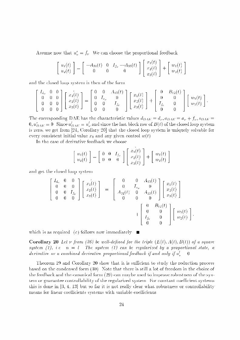
Assume now that u
r
�
= f
�
. We can choose the proportional feedback
"
u
1
(t)
u
2
(t)
#
=
"
�A
31
(t) 0 I
f
�
�A
33
(t)
0 0 0
#
2
6
4
x
1
(t)
x
2
(t)
x
3
(t)
3
7
5
+
"
w
1
(t)
w
2
(t)
#
and the closed loop system is then of the form
2
6
6
6
4
I
d
�
0 0
0 0 0
0 0 0
0 0 0
3
7
7
7
5
_
2
6
4
x
1
(t)
x
2
(t)
x
3
(t)
3
7
5
=
2
6
6
6
4
0 0 A
13
(t)
0 I
a
�
0
0 0 I
f
�
0 0 0
3
7
7
7
5
2
6
4
x
1
(t)
x
2
(t)
x
3
(t)
3
7
5
+
2
6
6
6
4
0 B
12
(t)
0 0
I
f
�
0
0 0
3
7
7
7
5
"
w
1
(t)
w
2
(t)
#
:
The corresponding DAE has the characteristic values d
DAE
= d
�
; a
DAE
= a
�
+ f
�
; s
DAE
=
0; u
r
DAE
= 0. Since u
l
DAE
= u
l
�
and since the last block row of B(t) of the closed loop system
is zero, we get from [24, Corollary 20] that the closed loop system is uniquely solvable for
every consistent initial value x
0
and any given control w(t).
In the case of derivative feedback we choose
"
u
1
(t)
u
2
(t)
#
=
"
0 0 I
f
�
0 0 0
#
_
2
6
4
x
1
(t)
x
2
(t)
x
3
(t)
3
7
5
+
"
w
1
(t)
w
2
(t)
#
and get the closed loop system
2
6
6
6
4
I
d
�
0 0
0 0 0
0 0 I
f
�
0 0 0
3
7
7
7
5
_
2
6
4
x
1
(t)
x
2
(t)
x
3
(t)
3
7
5
=
2
6
6
6
4
0 0 A
13
(t)
0 I
a
�
0
A
31
(t) 0 A
33
(t)
0 0 0
3
7
7
7
5
2
6
4
x
1
(t)
x
2
(t)
x
3
(t)
3
7
5
+
2
6
6
6
4
0 B
12
(t)
0 0
I
f
�
0
0 0
3
7
7
7
5
"
w
1
(t)
w
2
(t)
#
:
which is as required. (c) follows now immediately.
Corollary 20 Let � from (36) be well-de�ned for the triple (E(t); A(t); B(t)) of a square
system (1), i.e. n = l. The system (1) can be regularized by a proportional state, a
derivative or a combined derivative proportional feedback if and only if u
l
�
= 0.
Theorem 19 and Corollary 20 show that it is su�cient to study the reduction process
based on the condensed form (30). Note that there is still a lot of freedom in the choice of
the feedback and the canonical form (29) can maybe used to improve robustness of the sys-
tem or guarantee controllability of the regularized system. For constant coe�cient systems
this is done in [3, 4, 13] but so far it is not really clear what robustness or controllability
means for linear coe�cients systems with variable coe�cients.
24

6 Conclusion
We have presented local and global equivalences and corresponding canonical forms for
linear descriptor systems with variable coe�cients. The global canonical forms and the
global condensed forms, which are not as far reduced as the canonical forms, are powerful
tools in the analysis of this type of descriptor systems. Based on a condensed form we
found under what conditions a linear descriptor system is regularizable, i.e., there exists a
derivative and/or proportional state feedback such that the closed loop system is uniquely
solvable for all consistent initial vectors. These conditions are necessary and su�cient.
While the global forms are not suitable for numerical computations the numerical acces-
sibility of local quantities which give essential information on the global solution behaviour
are of great importance in the development of numerical methods.
We assumed that sequences of characteristic values are constant. As for di�erential
algebraic equations weaker assumptions such as jumps at isolated points connected with a
weak solvability concept can be considered.
A Proof of Theorem 10
To proof Theorem 10 we make use of the following property [21, 30]
Lemma 21 Let E 2 C
`
([t
1
; t
2
]; C
n;n
), ` 2 N
0
and rankE(t) = r for all t 2 [t
1
; t
2
]. Then
there exist U; V 2 C
`
([t
1
; t
2
]; C
n;n
) with U(t); V (t) nonsingular (unitary) for every t 2 [t
1
; t
2
]
such that
U(t)
�
E(t)V (t) =
"
�(t) 0
0 0
#
; t 2 [t
1
; t
2
]; (45)
where � 2 C
`
([t
1
; t
2
]; C
r;r
).
Proof of Theorem 10. From now on, we will omit the argument t in the proofs and
use the word "new" on top of the equivalence operator if we have changed the notation
according to the new block structure of the matrices. Using Lemma 21, we have
(E;A;B) � (U
�
1
�
1
V
1
; U
�
1
AV
1
� U
�
1
E
_
V
1
; U
�
1
B)
new
�
"
�
1
0
0 0
#
;
"
A
11
A
12
A
21
A
22
#
;
"
B
11
B
21
# !
new
�
"
I
r
0
0 0
#
;
"
A
11
A
12
A
21
A
22
#
;
"
B
11
B
21
# !
new
�
0
B
@
2
6
4
I
r
0
0 0
0 0
3
7
5;
2
6
4
A
11
A
12
A
21
A
22
A
31
A
32
3
7
5;
2
6
4
B
11
B
12
�
2
0
0 0
3
7
5
1
C
A
new
�
0
B
@
2
6
4
I
r
0
0 0
0 0
3
7
5;
2
6
4
A
11
A
12
A
21
A
22
A
31
A
32
3
7
5;
2
6
4
B
11
B
12
I
f
0
0 0
3
7
5
1
C
A
25

�
0
B
@
2
6
4
I
r
0
0 0
0 0
3
7
5
;
2
6
4
A
11
A
12
V
3
A
21
A
22
V
3
U
�
3
A
31
U
�
3
A
32
V
3
3
7
5
�
2
6
4
I
r
0
0 0
0 0
3
7
5
"
I
r
0
0
_
V
3
#
;
2
6
4
B
11
B
12
I
f
0
0 0
3
7
5
1
C
A
new
�
0
B
B
B
@
2
6
6
6
4
I
r
0 0
0 0 0
0 0 0
0 0 0
3
7
7
7
5
;
2
6
6
6
4
A
11
A
12
A
13
A
21
A
22
A
23
A
31
I
a
0
A
41
0 0
3
7
7
7
5
;
2
6
6
6
4
B
11
B
12
I
f
0
0 0
0 0
3
7
7
7
5
1
C
C
C
A
new
�
0
B
B
B
B
B
B
B
B
@
2
6
6
6
6
6
6
6
6
4
E
11
E
12
0 0 0
E
21
E
22
0 0 0
0 0 0 0 0
0 0 0 0 0
0 0 0 0 0
0 0 0 0 0
3
7
7
7
7
7
7
7
7
5
;
2
6
6
6
6
6
6
6
6
4
A
11
A
12
A
13
A
14
A
15
A
21
A
22
A
23
A
24
A
25
A
31
A
32
A
33
A
34
A
35
A
41
A
42
I
a
0 0
�
4
0 0 0 0
0 0 0 0 0
3
7
7
7
7
7
7
7
7
5
;
2
6
6
6
6
6
6
6
6
4
B
11
B
12
B
21
B
22
I
f
0
0 0
0 0
0 0
3
7
7
7
7
7
7
7
7
5
1
C
C
C
C
C
C
C
C
A
new
�
0
B
B
B
B
B
B
B
B
@
2
6
6
6
6
6
6
6
6
4
I
s
0 0 0 0
0 I
d
0 0 0
0 0 0 0 0
0 0 0 0 0
0 0 0 0 0
0 0 0 0 0
3
7
7
7
7
7
7
7
7
5
;
2
6
6
6
6
6
6
6
6
4
A
11
A
12
A
13
A
14
A
15
A
21
A
22
A
23
A
24
A
25
A
31
A
32
A
33
A
34
A
35
A
41
A
42
I
a
0 0
I
s
0 0 0 0
0 0 0 0 0
3
7
7
7
7
7
7
7
7
5
;
2
6
6
6
6
6
6
6
6
4
B
11
B
12
B
21
B
22
I
f
0
0 0
0 0
0 0
3
7
7
7
7
7
7
7
7
5
1
C
C
C
C
C
C
C
C
A
new
�
0
B
B
B
B
B
B
B
B
@
2
6
6
6
6
6
6
6
6
4
I
s
0 0 0 0
0 I
d
0 0 0
0 0 0 0 0
0 0 0 0 0
0 0 0 0 0
0 0 0 0 0
3
7
7
7
7
7
7
7
7
5
;
2
6
6
6
6
6
6
6
6
4
A
11
A
12
A
13
A
14
A
15
A
21
A
22
A
23
A
24
A
25
A
31
A
32
I
a
0 0
I
s
0 0 0 0
A
51
A
52
A
53
A
54
A
55
0 0 0 0 0
3
7
7
7
7
7
7
7
7
5
;
2
6
6
6
6
6
6
6
6
4
0 B
12
0 B
22
0 0
0 0
I
f
0
0 0
3
7
7
7
7
7
7
7
7
5
1
C
C
C
C
C
C
C
C
A
new
�
0
B
B
B
B
B
B
B
B
@
2
6
6
6
6
6
6
6
6
4
I
s
0 0 0 0
0 I
d
0 0 0
0 0 0 0 0
0 0 0 0 0
0 0 0 0 0
0 0 0 0 0
3
7
7
7
7
7
7
7
7
5
;
2
6
6
6
6
6
6
6
6
4
0 A
12
A
13
A
14
A
15
0 A
22
A
23
A
24
A
25
0 A
32
I
a
0 0
I
s
0 0 0 0
0 A
52
A
53
A
54
A
55
0 0 0 0 0
3
7
7
7
7
7
7
7
7
5
;
2
6
6
6
6
6
6
6
6
4
0 B
12
0 B
22
0 0
0 0
I
f
0
0 0
3
7
7
7
7
7
7
7
7
5
1
C
C
C
C
C
C
C
C
A
�
0
B
B
B
B
B
B
B
B
@
2
6
6
6
6
6
6
6
6
4
I
s
0 0 0 0
0 I
d
0 0 0
0 0 0 0 0
0 0 0 0 0
0 0 0 0 0
0 0 0 0 0
3
7
7
7
7
7
7
7
7
5
;
2
6
6
6
6
6
6
6
6
4
0 A
12
A
13
A
14
A
15
0 A
22
A
23
A
24
A
25
0 0 I
a
0 0
I
s
0 0 0 0
0 A
52
A
53
A
54
A
55
0 0 0 0 0
3
7
7
7
7
7
7
7
7
5
;
2
6
6
6
6
6
6
6
6
4
0 B
12
0 B
22
0 0
0 0
I
f
0
0 0
3
7
7
7
7
7
7
7
7
5
1
C
C
C
C
C
C
C
C
A
26

new
�
0
B
B
B
B
B
B
B
B
B
B
B
B
B
@
2
6
6
6
6
6
6
6
6
6
6
6
6
6
4
I
s
c
0 0 0 0 0 0
0 I
s
u
0 0 0 0 0
0 0 I
d
0 0 0 0
0 0 0 0 0 0 0
0 0 0 0 0 0 0
0 0 0 0 0 0 0
0 0 0 0 0 0 0
0 0 0 0 0 0 0
3
7
7
7
7
7
7
7
7
7
7
7
7
7
5
;
2
6
6
6
6
6
6
6
6
6
6
6
6
6
4
0 0 A
13
0 A
15
A
16
A
17
0 0 A
23
0 A
25
A
26
A
27
0 0 A
33
0 A
35
A
36
A
37
0 0 0 I
a
0 0 0
I
s
c
0 0 0 0 0 0
0 I
s
u
0 0 0 0 0
0 0 A
73
0 A
75
A
76
A
77
0 0 0 0 0 0 0
3
7
7
7
7
7
7
7
7
7
7
7
7
7
5
;
2
6
6
6
6
6
6
6
6
6
6
6
6
6
4
0 I
s
c
0
0 0 0
0 B
32
B
33
0 0 0
0 0 0
0 0 0
I
f
0 0
0 0 0
3
7
7
7
7
7
7
7
7
7
7
7
7
7
5
1
C
C
C
C
C
C
C
C
C
C
C
C
C
A
new
�
0
B
B
B
B
B
B
B
B
B
B
B
B
B
@
2
6
6
6
6
6
6
6
6
6
6
6
6
6
4
I
s
c
0 0 0 0 0 0
0 I
s
u
0 0 0 0 0
�B
32
0 I
d
0 0 0 0
0 0 0 0 0 0 0
0 0 0 0 0 0 0
0 0 0 0 0 0 0
0 0 0 0 0 0 0
0 0 0 0 0 0 0
3
7
7
7
7
7
7
7
7
7
7
7
7
7
5
;
2
6
6
6
6
6
6
6
6
6
6
6
6
6
4
0 0 A
13
0 A
15
A
16
A
17
0 0 A
23
0 A
25
A
26
A
27
0 0 A
33
0 A
35
A
36
A
37
0 0 0 I
a
0 0 0
I
s
c0 0 0 0 0 0
0 I
s
u
0 0 0 0 0
0 0 A
73
0 A
75
A
76
A
77
0 0 0 0 0 0 0
3
7
7
7
7
7
7
7
7
7
7
7
7
7
5
;
2
6
6
6
6
6
6
6
6
6
6
6
6
6
4
0 I
s
c
0
0 0 0
0 0 B
33
0 0 0
0 0 0
0 0 0
I
f
0 0
0 0 0
3
7
7
7
7
7
7
7
7
7
7
7
7
7
5
1
C
C
C
C
C
C
C
C
C
C
C
C
C
A
27

new
�
0
B
B
B
B
B
B
B
B
B
B
B
B
B
@
2
6
6
6
6
6
6
6
6
6
6
6
6
6
4
I
s
c
0 0 0 0 0 0
0 I
s
u
0 0 0 0 0
0 0 I
d
0 0 0 0
0 0 0 0 0 0 0
0 0 0 0 0 0 0
0 0 0 0 0 0 0
0 0 0 0 0 0 0
0 0 0 0 0 0 0
3
7
7
7
7
7
7
7
7
7
7
7
7
7
5
;
2
6
6
6
6
6
6
6
6
6
6
6
6
6
4
A
11
0 A
13
0 A
15
A
16
A
17
A
21
0 A
23
0 A
25
A
26
A
27
A
31
0 A
33
0 A
35
A
36
A
37
0 0 0 I
a
0 0 0
I
s
c
0 0 0 0 0 0
0 I
s
u
0 0 0 0 0
A
71
0 A
73
0 A
75
A
76
A
77
0 0 0 0 0 0 0
3
7
7
7
7
7
7
7
7
7
7
7
7
7
5
;
2
6
6
6
6
6
6
6
6
6
6
6
6
6
4
0 I
s
c
0
0 0 0
0 0 B
33
0 0 0
0 0 0
0 0 0
I
f
0 0
0 0 0
3
7
7
7
7
7
7
7
7
7
7
7
7
7
5
1
C
C
C
C
C
C
C
C
C
C
C
C
C
A
�
0
B
B
B
B
B
B
B
B
B
B
B
B
B
@
2
6
6
6
6
6
6
6
6
6
6
6
6
6
4
I
s
c
0 0 0 0 0 0
0 I
s
u
0 0 0 0 0
0 0 I
d
0 0 0 0
0 0 0 0 0 0 0
0 0 0 0 0 0 0
0 0 0 0 0 0 0
0 0 0 0 0 0 0
0 0 0 0 0 0 0
3
7
7
7
7
7
7
7
7
7
7
7
7
7
5
;
2
6
6
6
6
6
6
6
6
6
6
6
6
6
4
0 0 A
13
0 A
15
A
16
A
17
0 0 A
23
0 A
25
A
26
A
27
0 0 A
33
0 A
35
A
36
A
37
0 0 I
a
0 0 0 0
I
s
c0 0 0 0 0 0
0 I
s
u
0 0 0 0 0
0 0 A
73
0 A
75
A
76
A
77
0 0 0 0 0 0 0
3
7
7
7
7
7
7
7
7
7
7
7
7
7
5
;
2
6
6
6
6
6
6
6
6
6
6
6
6
6
4
0 I
s
c
0
0 0 0
0 0 B
33
0 0 0
0 0 0
0 0 0
I
f
0 0
0 0 0
3
7
7
7
7
7
7
7
7
7
7
7
7
7
5
1
C
C
C
C
C
C
C
C
C
C
C
C
C
A
28

new
�
0
B
B
B
B
B
B
B
B
B
B
B
B
B
B
B
@
2
6
6
6
6
6
6
6
6
6
6
6
6
6
6
6
4
I
s
c
0 0 0 0 0 0 0
0 I
s
u
0 0 0 0 0 0
0 0 I
d
c
0 0 0 0 0
0 0 0 I
d
u
0 0 0 0
0 0 0 0 0 0 0 0
0 0 0 0 0 0 0 0
0 0 0 0 0 0 0 0
0 0 0 0 0 0 0 0
0 0 0 0 0 0 0 0
3
7
7
7
7
7
7
7
7
7
7
7
7
7
7
7
5
;
2
6
6
6
6
6
6
6
6
6
6
6
6
6
6
6
4
0 0 A
13
A
14
0 A
16
A
17
A
18
0 0 A
23
A
24
0 A
26
A
27
A
28
0 0 A
33
A
34
0 A
36
A
37
A
38
0 0 A
43
A
44
0 A
46
A
47
A
48
0 0 0 0 I
a
0 0 0
I
s
c
0 0 0 0 0 0 0
0 I
s
u
0 0 0 0 0 0
0 0 A
83
A
83
0 A
86
A
87
A
88
0 0 0 0 0 0 0 0
3
7
7
7
7
7
7
7
7
7
7
7
7
7
7
7
5
;
2
6
6
6
6
6
6
6
6
6
6
6
6
6
6
6
4
0 I
s
c
0
0 0 0
0 0 I
d
c
0 0 0
0 0 0
0 0 0
0 0 0
I
f
0 0
0 0 0
3
7
7
7
7
7
7
7
7
7
7
7
7
7
7
7
5
1
C
C
C
C
C
C
C
C
C
C
C
C
C
C
C
A
�
0
B
B
B
B
B
B
B
B
B
B
B
B
B
B
B
@
2
6
6
6
6
6
6
6
6
6
6
6
6
6
6
6
4
I
s
c
0 0 0 0 0 0 0
0 I
s
u
0 0 0 0 0 0
0 0 Q
5
0 0 0 0 0
0 0 0 I
d
u
0 0 0 0
0 0 0 0 0 0 0 0
0 0 0 0 0 0 0 0
0 0 0 0 0 0 0 0
0 0 0 0 0 0 0 0
0 0 0 0 0 0 0 0
3
7
7
7
7
7
7
7
7
7
7
7
7
7
7
7
5
;
2
6
6
6
6
6
6
6
6
6
6
6
6
6
6
6
6
4
0 0 A
13
A
14
0 A
16
A
17
A
18
0 0 A
23
A
24
0 A
26
A
27
A
28
0 0 A
33
Q
5
�
_
Q
5
A
34
0 A
36
A
37
A
38
0 0 A
43
A
44
0 A
46
A
47
A
48
0 0 0 0 I
a
0 0 0
I
s
c0 0 0 0 0 0 0
0 I
s
u
0 0 0 0 0 0
0 0 A
83
A
83
0 A
86
A
87
A
88
0 0 0 0 0 0 0 0
3
7
7
7
7
7
7
7
7
7
7
7
7
7
7
7
7
5
;
2
6
6
6
6
6
6
6
6
6
6
6
6
6
6
6
4
0 I
s
c
0
0 0 0
0 0 I
d
c
0 0 0
0 0 0
0 0 0
0 0 0
I
f
0 0
0 0 0
3
7
7
7
7
7
7
7
7
7
7
7
7
7
7
7
5
1
C
C
C
C
C
C
C
C
C
C
C
C
C
C
C
C
A
Q
5
was chosen to be the solution of the initial value problem
_
Q
5
�A
33
Q
5
; Q
5
(t
0
) = I;
29

which is nonsingular at every point t 2 [t
1
; t
2
], i.e.
(E;A;B)
new
�
0
B
B
B
B
B
B
B
B
B
B
B
B
B
B
B
@
2
6
6
6
6
6
6
6
6
6
6
6
6
6
6
6
4
I
s
c
0 0 0 0 0 0 0
0 I
s
u
0 0 0 0 0 0
0 0 I
d
c
0 0 0 0 0
0 0 0 I
d
u
0 0 0 0
0 0 0 0 0 0 0 0
0 0 0 0 0 0 0 0
0 0 0 0 0 0 0 0
0 0 0 0 0 0 0 0
0 0 0 0 0 0 0 0
3
7
7
7
7
7
7
7
7
7
7
7
7
7
7
7
5
;
2
6
6
6
6
6
6
6
6
6
6
6
6
6
6
6
4
0 0 A
13
A
14
0 A
16
A
17
A
18
0 0 A
23
A
24
0 A
26
A
27
A
28
0 0 0 A
34
0 A
36
A
37
A
38
0 0 A
43
A
44
0 A
46
A
47
A
48
0 0 0 0 I
a
0 0 0
I
s
c
0 0 0 0 0 0 0
0 I
s
u
0 0 0 0 0 0
0 0 A
83
A
83
0 A
86
A
87
A
88
0 0 0 0 0 0 0 0
3
7
7
7
7
7
7
7
7
7
7
7
7
7
7
7
5
;
2
6
6
6
6
6
6
6
6
6
6
6
6
6
6
6
4
0 I
s
c
0
0 0 0
0 0 I
d
c
0 0 0
0 0 0
0 0 0
0 0 0
I
f
0 0
0 0 0
3
7
7
7
7
7
7
7
7
7
7
7
7
7
7
7
5
1
C
C
C
C
C
C
C
C
C
C
C
C
C
C
C
A
which at last leads to (29) by a similar �nal transformation step.
B Proof of Theorem 15
From
rank(R
i�1
(t)
�
[A
(i�1)
12
(t)A
(i�1)
14
(t)A
(i�1)
15
(t)])
= rank(R
i�1
(t)
�
[A
(i�1)
14
(t)A
(i�1)
14
(t)]) + rank(W
i�1
(t)
�
R
i�1
(t)
�
A
(i�1)
12
(t))
we obtain (39a), while (39b,c) are consequences of Lemma 14 (35f,g).
Starting from Corollary 11 in the permuted form (if we do not perform the last elimi-
nation step, i.e. do not zero out A
22
)
0
B
B
B
B
B
B
B
B
@
2
6
6
6
6
6
6
6
6
4
I 0 0 0 0
0 0 0 I 0
0 0 0 0 0
0 0 0 0 0
0 0 0 0 0
0 0 0 0 0
3
7
7
7
7
7
7
7
7
5
;
2
6
6
6
6
6
6
6
6
4
A
11
A
12
A
13
0 0
A
21
A
22
A
23
0 0
0 0 0 0 0
0 0 0 I 0
0 0 0 0 I
A
61
A
62
A
63
0 0
3
7
7
7
7
7
7
7
7
5
;
2
6
6
6
6
6
6
6
6
4
0 B
12
0 B
22
0 0
0 0
0 0
I 0
3
7
7
7
7
7
7
7
7
5
1
C
C
C
C
C
C
C
C
A
d
0
s
0
w
l
0
s
0
b
0
f
0
30

we obtain the following equivalent triples of matrix functions in the i{th step (omitting
subscripts
(i)
and denoting by [A
ij
: : :A
ij
] a block entry A
ij
which extends over several block
columns)
0
B
B
B
B
B
B
B
B
B
B
B
B
B
B
B
B
B
B
B
B
B
B
B
@
2
6
6
6
6
6
6
6
6
6
6
6
6
6
6
6
6
6
6
6
6
6
6
6
4
I 0 0 : : : : : : : : : 0 0 0 � : : : : : : �
0 0 0 : : : : : : : : : 0 I 0 � : : : : : : �
0 F
i
�
.
.
.
0
.
.
.
.
.
.
.
.
.
.
.
.
.
.
.
.
.
.
F
1
0 0
0 0 W
11
� : : : �
0 0 W
21
� : : : �
0 E
i�1
�
.
.
.
.
.
.
.
.
.
E
1
0
0 0 � : : : : : : �
3
7
7
7
7
7
7
7
7
7
7
7
7
7
7
7
7
7
7
7
7
7
7
7
5
2
6
6
6
6
6
6
6
6
6
6
6
6
6
6
6
6
6
6
6
6
6
6
6
4
A
11
A
12
A
13
: : : : : : : : : A
13
A
21
A
22
A
23
: : : : : : : : : A
23
0
.
.
.
.
.
.
.
.
.
0
I 0
0 I
I
.
.
.
.
.
.
I
� � � : : : : : : : : : � 0 0 0 : : : : : : 0
3
7
7
7
7
7
7
7
7
7
7
7
7
7
7
7
7
7
7
7
7
7
7
7
5
;
2
6
6
6
6
6
6
6
6
6
6
6
6
6
6
6
6
6
6
6
6
6
6
6
4
0 B
12
0 B
22
0 0
.
.
.
.
.
.
.
.
.
.
.
.
.
.
.
.
.
.
0 0
0 0
0 0
0 0
.
.
.
.
.
.
.
.
.
.
.
.
0 0
I 0
3
7
7
7
7
7
7
7
7
7
7
7
7
7
7
7
7
7
7
7
7
7
7
7
5
1
C
C
C
C
C
C
C
C
C
C
C
C
C
C
C
C
C
C
C
C
C
C
C
A
d
i
s
i
w
l
i
.
.
.
.
.
.
.
.
.
w
l
0
s
i
b
i
c
i�1
.
.
.
.
.
.
c
0
f
i
31

new
�
0
B
B
B
B
B
B
B
B
B
B
B
B
B
B
B
B
B
B
B
B
B
B
B
B
B
B
@
2
6
6
6
6
6
6
6
6
6
6
6
6
6
6
6
6
6
6
6
6
6
6
6
6
6
6
4
I 0 0 0 : : : : : : : : : 0 0 0 0 � : : : : : : �
0 0 0 0 : : : : : : : : : 0 I 0 0 � : : : : : : �
0 0 0 0 : : : : : : : : : 0 0 I 0 � : : : : : : �
0 F
i
�
.
.
.
0
.
.
.
.
.
.
.
.
.
.
.
.
.
.
.
.
.
.
F
1
0 0
0 0 0 W
11
� : : : �
0 0 0 W
21
� : : : �
0 0 0 W
31
� : : : �
0 E
i�1
�
.
.
.
.
.
.
.
.
.
E
1
0
0 0 0 � : : : : : : �
3
7
7
7
7
7
7
7
7
7
7
7
7
7
7
7
7
7
7
7
7
7
7
7
7
7
7
5
2
6
6
6
6
6
6
6
6
6
6
6
6
6
6
6
6
6
6
6
6
6
6
6
6
6
6
4
A
11
A
12
A
13
A
14
: : : : : : : : : A
14
A
21
A
22
A
23
A
24
: : : : : : : : : A
24
A
31
A
32
A
33
A
34
: : : : : : : : : A
34
0
.
.
.
.
.
.
.
.
.
0
I 0 0
0 I 0
0 0 I
I
.
.
.
.
.
.
I
� � � � : : : : : : : : : � 0 0 0 0 : : : : : : 0
3
7
7
7
7
7
7
7
7
7
7
7
7
7
7
7
7
7
7
7
7
7
7
7
7
7
7
5
;
2
6
6
6
6
6
6
6
6
6
6
6
6
6
6
6
6
6
6
6
6
6
6
6
6
6
6
4
0 B
12
B
13
0 I 0
0 0 0
0 0 0
.
.
.
.
.
.
.
.
.
.
.
.
.
.
.
.
.
.
0 0 0
0 0 0
0 0 0
0 0 0
0 0 0
.
.
.
.
.
.
.
.
.
.
.
.
0 0 0
I 0 0
3
7
7
7
7
7
7
7
7
7
7
7
7
7
7
7
7
7
7
7
7
7
7
7
7
7
7
5
1
C
C
C
C
C
C
C
C
C
C
C
C
C
C
C
C
C
C
C
C
C
C
C
C
C
C
A
d
i
g
i+1
s
i
� g
i+1
w
l
i
.
.
.
.
.
.
.
.
.
w
l
0
g
i+1
s
i
� g
i+1
b
i
c
i�1
.
.
.
.
.
.
c
0
f
i
32

new
�
0
B
B
B
B
B
B
B
B
B
B
B
B
B
B
B
B
B
B
B
B
B
B
B
B
B
@
2
6
6
6
6
6
6
6
6
6
6
6
6
6
6
6
6
6
6
6
6
6
6
6
6
6
4
I 0 0 : : : : : : : : : 0 0 0 0 � : : : : : : �
0 0 0 : : : : : : : : : 0 0 I 0 � : : : : : : �
0 F
i
�
.
.
.
0
.
.
.
.
.
.
.
.
.
.
.
.
.
.
.
.
.
.
F
1
0 0
0 0 0 W
11
� : : : �
0 0 0 W
21
� : : : �
0 0 0 W
31
� : : : �
0 E
i�1
�
.
.
.
.
.
.
.
.
.
E
1
0
� 0 0 � : : : : : : �
3
7
7
7
7
7
7
7
7
7
7
7
7
7
7
7
7
7
7
7
7
7
7
7
7
7
5
;
2
6
6
6
6
6
6
6
6
6
6
6
6
6
6
6
6
6
6
6
6
6
6
6
6
6
4
A
11
A
12
A
13
: : : : : : : : : A
13
A
21
A
22
A
23
: : : : : : : : : A
23
0
.
.
.
.
.
.
.
.
.
0
I 0 0
0 I 0
0 0 I
I
.
.
.
.
.
.
I
� � � : : : : : : : : : � 0 0 0 0 : : : : : : 0
3
7
7
7
7
7
7
7
7
7
7
7
7
7
7
7
7
7
7
7
7
7
7
7
7
7
5
;
2
6
6
6
6
6
6
6
6
6
6
6
6
6
6
6
6
6
6
6
6
6
6
6
6
6
4
0 B
12
0 0
0 0
.
.
.
.
.
.
.
.
.
.
.
.
.
.
.
.
.
.
0 0
0 0
0 0
0 0
0 0
.
.
.
.
.
.
.
.
.
.
.
.
0 0
I 0
3
7
7
7
7
7
7
7
7
7
7
7
7
7
7
7
7
7
7
7
7
7
7
7
7
7
5
1
C
C
C
C
C
C
C
C
C
C
C
C
C
C
C
C
C
C
C
C
C
C
C
C
C
A
d
i
s
i
� g
i+1
w
l
i
.
.
.
.
.
.
.
.
.
w
l
0
g
i+1
s
i
� g
i+1
b
i
c
i�1
.
.
.
.
.
.
c
0
f
i+1
33

new
�
0
B
B
B
B
B
B
B
B
B
B
B
B
B
B
B
B
B
B
B
B
B
B
B
B
B
B
B
B
B
B
@
2
6
6
6
6
6
6
6
6
6
6
6
6
6
6
6
6
6
6
6
6
6
6
6
6
6
6
6
6
6
6
4
I 0 0 0 : : : : : : : : : 0 0 0 0 0 � : : : : : : �
0 0 0 0 : : : : : : : : : 0 0 U
11
U
12
0 � : : : : : : �
0 0 0 0 : : : : : : : : : 0 0 U
21
U
22
0 � : : : : : : �
0 F
i
�
.
.
.
0
.
.
.
.
.
.
.
.
.
.
.
.
.
.
.
.
.
.
F
1
0 0
0 W
11
� : : : �
.
.
.
W
21
� : : : �
.
.
.
W
31
� : : : �
0 W
41
� : : : �
0 E
i�1
�
.
.
.
.
.
.
.
.
.
E
1
0
� 0 0 0 � : : : : : : �
3
7
7
7
7
7
7
7
7
7
7
7
7
7
7
7
7
7
7
7
7
7
7
7
7
7
7
7
7
7
7
5
;
2
6
6
6
6
6
6
6
6
6
6
6
6
6
6
6
6
6
6
6
6
6
6
6
6
6
6
6
6
4
A
11
A
12
A
13
A
14
: : : : : : : : : A
14
A
21
I 0 0 : : : : : : : : : 0
A
31
0 0 0 : : : : : : : : : 0
0
.
.
.
.
.
.
.
.
.
0
I
I
I
I
I
.
.
.
.
.
.
I
� � � � : : : : : : : : : � 0 0 0 0 0 : : : : : : 0
3
7
7
7
7
7
7
7
7
7
7
7
7
7
7
7
7
7
7
7
7
7
7
7
7
7
7
7
7
5
;
2
6
6
6
6
6
6
6
6
6
6
6
6
6
6
6
6
6
6
6
6
6
6
6
6
6
6
6
6
4
0 B
12
0 0
0 0
0 0
.
.
.
.
.
.
.
.
.
.
.
.
.
.
.
.
.
.
0 0
0 0
0 0
0 0
0 0
0 0
.
.
.
.
.
.
.
.
.
.
.
.
0 0
I 0
3
7
7
7
7
7
7
7
7
7
7
7
7
7
7
7
7
7
7
7
7
7
7
7
7
7
7
7
7
5
1
C
C
C
C
C
C
C
C
C
C
C
C
C
C
C
C
C
C
C
C
C
C
C
C
C
C
C
C
A
d
i
b
i+1
s
i
� g
i+1
� b
i+1
w
l
i
.
.
.
.
.
.
.
.
.
w
l
0
g
i+1
b
i+1
s
i
� g
i+1
� b
i+1
b
i
c
i�1
.
.
.
.
.
.
c
0
f
i+1
34

new
�
0
B
B
B
B
B
B
B
B
B
B
B
B
B
B
B
B
B
B
B
B
B
B
B
B
B
B
@
2
6
6
6
6
6
6
6
6
6
6
6
6
6
6
6
6
6
6
6
6
6
6
6
6
6
6
4
I 0 0 0 0 : : : : : : : : : 0 0 � : : : : : : �
0 I 0 0 0 : : : : : : : : : 0 0 � : : : : : : �
0 0 0 0 0 : : : : : : : : : 0 U
11
� : : : : : : �
0 0 0 0 0 : : : : : : : : : 0 U
21
� : : : : : : �
0 0 0 0 0 : : : : : : : : : 0 U
31
� : : : : : : �
0 F
i
�
.
.
.
0
.
.
.
.
.
.
.
.
.
.
.
.
.
.
.
.
.
.
F
1
0 0
0 E
i
� : : : �
0 E
i�1
�
.
.
.
.
.
.
.
.
.
E
1
0
� � : : : : : : �
3
7
7
7
7
7
7
7
7
7
7
7
7
7
7
7
7
7
7
7
7
7
7
7
7
7
7
5
;
2
6
6
6
6
6
6
6
6
6
6
6
6
6
6
6
6
6
6
6
6
6
6
6
6
6
6
4
A
11
A
12
A
13
A
14
A
15
: : : : : : : : : A
15
A
21
A
22
A
23
A
24
A
25
: : : : : : : : : A
25
A
31
A
41
I 0 0 : : : : : : : : : 0
0 I 0 0 0 : : : : : : : : : 0
0 0 0 0 0 : : : : : : : : : 0
0
.
.
.
.
.
.
.
.
.
0
I
I
.
.
.
.
.
.
I
� � � � � : : : : : : : : : � 0 0 : : : : : : 0
3
7
7
7
7
7
7
7
7
7
7
7
7
7
7
7
7
7
7
7
7
7
7
7
7
7
7
5
;
2
6
6
6
6
6
6
6
6
6
6
6
6
6
6
6
6
6
6
6
6
6
6
6
6
6
6
4
0 B
12
0 0
0 0
0 0
0 0
0 0
.
.
.
.
.
.
.
.
.
.
.
.
.
.
.
.
.
.
0 0
0 0
0 0
.
.
.
.
.
.
.
.
.
.
.
.
0 0
I 0
3
7
7
7
7
7
7
7
7
7
7
7
7
7
7
7
7
7
7
7
7
7
7
7
7
7
7
5
1
C
C
C
C
C
C
C
C
C
C
C
C
C
C
C
C
C
C
C
C
C
C
C
C
C
C
A
d
i+1
s
i+1
b
i+1
s
i+1
w
l
i+1
w
l
i
.
.
.
.
.
.
.
.
.
w
l
0
c
i
c
i�1
.
.
.
.
.
.
c
0
f
i+1
35

new
�
0
B
B
B
B
B
B
B
B
B
B
B
B
B
B
B
B
B
B
B
B
B
B
B
B
B
B
@
2
6
6
6
6
6
6
6
6
6
6
6
6
6
6
6
6
6
6
6
6
6
6
6
6
6
6
4
I 0 0 0 0 : : : : : : : : : 0 � � : : : : : : �
0 I 0 0 0 : : : : : : : : : 0 � � : : : : : : �
0 0 0 0 0 : : : : : : : : : 0 W
21
� : : : : : : �
0 0 0 0 0 : : : : : : : : : 0 W
11
� : : : : : : �
0 0 0 0 0 : : : : : : : : : 0 F
i+1
� : : : : : : �
0 F
i
�
.
.
.
0
.
.
.
.
.
.
.
.
.
.
.
.
.
.
.
.
.
.
F
1
0 0
0 E
i
� : : : �
0 E
i�1
�
.
.
.
.
.
.
.
.
.
E
1
0
� � : : : : : : �
3
7
7
7
7
7
7
7
7
7
7
7
7
7
7
7
7
7
7
7
7
7
7
7
7
7
7
5
;
2
6
6
6
6
6
6
6
6
6
6
6
6
6
6
6
6
6
6
6
6
6
6
6
6
6
6
4
A
11
0 0 A
14
A
15
: : : : : : : : : A
15
A
21
0 0 A
24
A
25
: : : : : : : : : A
25
0 0 I 0 0 : : : : : : : : : 0
0 I 0 0 0 : : : : : : : : : 0
0 0 0 0 0 : : : : : : : : : 0
0
.
.
.
.
.
.
.
.
.
0
I
I
.
.
.
.
.
.
I
� 0 0 � � : : : : : : : : : � 0 0 : : : : : : 0
3
7
7
7
7
7
7
7
7
7
7
7
7
7
7
7
7
7
7
7
7
7
7
7
7
7
7
5
;
2
6
6
6
6
6
6
6
6
6
6
6
6
6
6
6
6
6
6
6
6
6
6
6
6
6
6
4
0 B
12
0 0
0 0
0 0
0 0
0 0
.
.
.
.
.
.
.
.
.
.
.
.
.
.
.
.
.
.
0 0
0 0
0 0
.
.
.
.
.
.
.
.
.
.
.
.
0 0
I 0
3
7
7
7
7
7
7
7
7
7
7
7
7
7
7
7
7
7
7
7
7
7
7
7
7
7
7
5
1
C
C
C
C
C
C
C
C
C
C
C
C
C
C
C
C
C
C
C
C
C
C
C
C
C
C
A
d
i+1
s
i+1
b
i+1
s
i+1
w
l
i+1
w
l
i
.
.
.
.
.
.
.
.
.
w
l
0
c
i
c
i�1
.
.
.
.
.
.
c
0
f
i+1
36

new
�
0
B
B
B
B
B
B
B
B
B
B
B
B
B
B
B
B
B
B
B
B
B
B
@
2
6
6
6
6
6
6
6
6
6
6
6
6
6
6
6
6
6
6
6
6
6
6
4
I 0 0 0 : : : : : : 0 0 0 � � : : : �
0 0 0 0 : : : : : : 0 I 0 � � : : : �
0 0 0 F
i+1
� : : : �
0 0 F
i
�
.
.
.
.
.
.
.
.
.
.
.
.
.
.
.
F
1
0 0
0 0 0 0 : : : : : : : : : 0 0 W
11
� : : : �
0 0 0 0 : : : : : : : : : 0 0 W
21
� : : : �
0 E
i
�
.
.
.
.
.
.
.
.
.
E
1
0
� � : : : �
3
7
7
7
7
7
7
7
7
7
7
7
7
7
7
7
7
7
7
7
7
7
7
5
2
6
6
6
6
6
6
6
6
6
6
6
6
6
6
6
6
6
6
6
6
6
6
6
4
A
11
A
12
A
13
A
14
: : : : : : A
14
A
21
A
22
A
23
A
24
: : : : : : A
24
0
.
.
.
.
.
.
.
.
.
0
I
I
I
.
.
.
.
.
.
I
� � � � : : : : : : � 0 0 0 : : : : : : 0
3
7
7
7
7
7
7
7
7
7
7
7
7
7
7
7
7
7
7
7
7
7
7
7
5
;
2
6
6
6
6
6
6
6
6
6
6
6
6
6
6
6
6
6
6
6
6
6
6
6
4
0 B
12
0 0
0 0
.
.
.
.
.
.
.
.
.
.
.
.
.
.
.
.
.
.
0 0
0 0
0 0
0 0
.
.
.
.
.
.
.
.
.
.
.
.
0 0
I 0
3
7
7
7
7
7
7
7
7
7
7
7
7
7
7
7
7
7
7
7
7
7
7
7
5
1
C
C
C
C
C
C
C
C
C
C
C
C
C
C
C
C
C
C
C
C
C
C
C
A
d
i+1
s
i+1
w
l
i+1
.
.
.
.
.
.
.
.
.
w
l
0
s
i+1
b
i+1
c
i
c
i�1
.
.
.
c
0
f
i+1
Thus (40) follows by induction and (41) holds, since
"
F
i+1
E
i+1
#
is obtained by nonsingular
transformations applied to [0 U 0], with nonsingular U , where U is the transformation used
above in the third step.
References
[1] K. E. Brenan, S. L. Campbell, and L. R. Petzold. Numerical Solution of Initial-Value
Problems in Di�erential Algebraic Equations. Elsevier, North Holland, New York, N.
Y., 1989.
[2] A. Bunse-Gerstner, R. Byers, V. Mehrmann, and N. K. Nichols. Numerical computa-
tion of an analytic singular value decomposition of a matrix valued function. Numer.
Math., 60:1{40, 1991.
37

[3] A. Bunse-Gerstner, V. Mehrmann, and N. K. Nichols. Regularization of descriptor
systems by derivative and proportional state feedback. SIAM J. Matrix. Anal. Appl.,
13(1):46{67, 1992.
[4] A. Bunse-Gerstner, V. Mehrmann, and N. K. Nichols. Regularization of descriptor
systems by output feedback. IEEE Trans. Automat Control, 39(8):1742{1748, 1994.
[5] R. Byers, T. Geerts, and V. Mehrmann. Descriptor systems without controllabil-
ity at in�nity. Preprint, Fakult�at f�ur Mathematik, TU Chemnitz-Zwickau, D-09107
Chemnitz, FRG, November 1993.
[6] R. Byers, P. Kunkel, and V. Mehrmann. Regularization of linear descriptor systems
with variable coe�cients. Preprint, Fakult�at f�ur Mathematik, TU Chemnitz-Zwickau,
09107 Chemnitz, FRG, September 1994.
[7] S. L. Campbell. Singular Systems of Di�erential Equations. Pitman, San Francisco,
1980.
[8] S. L. Campbell. A general form for solvable linear time varying singular systems of
di�erential equations. SIAM J. Math. Anal., 18:1101{1115, 1987.
[9] S. L. Campbell. The numerical solution of higher index linear time varying singular
systems of di�erential equations. SIAM J. Sci. Statist. Comput., 6:334{348, 1988.
[10] S. L. Campbell. Linearization of DAEs along trajectories. Technical report, De-
partment of Mathematics, North Carolina State University, Raleigh, NC 27695-8205,
August 1993. To appear in in Zeitschrift f�ur angewandte Mathematik und Physik.
[11] S. L. Campbell, N. K. Nichols, and W. J. Terrell. Duality, observability, and control-
lability for linear time-varying descriptor systems. Circuits Systems Signal Process.,
10(4):455{470, 1991.
[12] S. L. Campbell and W. J. Terrell. Observability of linear time varying descriptor
systems. SIAM J. Matrix. Anal. Appl., 12:484{496, 1991.
[13] L. Elsner, C. He, and V. Mehrmann. Completion of a matrix so that the inverse has
minimum norm. application to the regularization of descriptor control problems. In
P. Van Dooren and B. Wyman, editors, Linear Algebra for Control Theory, pages
75{86. Springer Verlag, New York, 1993.
[14] F. R. Gantmacher. The Theory of Matrices, volume II. Chelsea Publishing Company,
New York, N.Y., 1964.
[15] C. W. Gear and L. R. Petzold. Di�erential/algebraic systems and matrix pencils. In
B. K�agstr�om and A. Ruhe, editors, Matrix Pencils, volume 973 of Lecture Notes in
Mathematics, pages 75{89. Springer-Verlag, 1983.
38

[16] T. Geerts. Solvability conditions, consistency, and weak consistency for linear
di�erential-algebraic equations and time-invariant linear systems: The general case.
Linear Algebra Appl., 181:111{130, 1993.
[17] T. Geerts and V. Mehrmann. Linear di�erential equations with constant coe�cients:
A distributional approach. Report 90-073, Sonderforschungsbereich 343, 'Diskrete
Strukturen in der Mathematik', Universit�at Bielefeld, Bielefeld, FRG, 1990.
[18] E. Griepentrog and R. M�arz. Di�erential-Algebraic Equations and Their Numerical
Treatment. Teubner-Texte zur Mathematik, Band 88, 1986.
[19] M. G�unther and P. Rentrop. Multirate row-methods and latency of electric cir-
cuits. Technical Report TUM-M9208, Mathematisches Institut, Technische Univer-
sit�at M�unchen, September 1992.
[20] E. Hairer and G. Wanner. Solving Ordinary Di�erential Equations II. Springer-Verlag,
Berlin, 1991.
[21] P. Kunkel and V. Mehrmann. Smooth factorizations of matrix valued functions and
their derivatives. Numer. Math., 60:115{132, 1991.
[22] P. Kunkel and V. Mehrmann. Canonical forms for linear di�erential-algebraic equa-
tions with variable coe�cients. Technical Report 69, Institut f�ur Geometrie und Prak-
tische Mathematik, RWTH Aachen, Templergraben 55, D-5100 Aachen, FRG, 1992.
To appear in J. Comp. Appl. Math.
[23] P. Kunkel and V. Mehrmann. A new class of discretization methods for the solution
of linear di�erential-algebraic equations. Materialien LXII , FSP Mathematisierung,
Universit�at Bielefeld, 1992. To appear in SIAM J. Numer. Anal.
[24] P. Kunkel and V. Mehrmann. A new look at pencils of matrix valued functions. Linear
Algebra Appl., 212/213:215{248, 1994.
[25] J. J. Loiseau, K.
�
Oz�caldiran, M. Malabre, and N. Karcanias. Feedback canonical forms
of singular systems. Kybernetika, 27(289-305), 1991.
[26] V. Mehrmann and W. Rath. Numerical methods for the computation of analytic sin-
gular value decompositions. Electronic Transaction on Numerical Analysis (ETNA),
1:72{88, 1993.
[27] P. J. Rabier and W. C. Rheinboldt. On impasse points of quasilinear di�erential
algebraic equations. Technical Report ICMA-92-171, Department of Mathematics
and Statistics, University of Pittsburgh, Pittsburgh, PA 15260, 1992.
39

[28] P. J. Rabier and W. C. Rheinboldt. Classical and generalized solutions of time-
dependent linear di�erential algebraic equations. Technical Report ICMA-93-183,
Dept. of Mathematics and Statistics, Univ. of Pittsburgh, Pittsburgh, PA 15260, USA,
1993. To appear in Lin. Alg. Appl.
[29] P. J. Rabier and W. C. Rheinboldt. Time-dependent linear DAE's with discontinous
input. Technical Report ICMA-94-186, Dept. of Mathematics and Statistics, Univ. of
Pittsburgh, Pittsburgh, PA 15260, USA, 1993. To appear in Lin. Alg. Appl.
[30] W. C. Rheinboldt. On the computation of multi-dimensional solution manifolds of
parameterized equations. Numer. Math., 53:165{181, 1988.
[31] T. Schmidt and M. Hou. Rollringgetriebe. Internal Report, Sicherheitstechnische Re-
gelungs- und Me�technik, Bergische Universit�at, GH Wuppertal, Wuppertal, FRG,
1992.
[32] B. Simeon, F. Grupp, C. F�uhrer, and P. Rentrop. A nonlinear truck model and its
treatment as a multibody system. Technical Report TUM-M9204, Mathematisches
Institut, TU M�unchen, M�unchen, FRG, 1992.
[33] P. Van Dooren. The computation of Kronecker's canonical form of a singular pencil.
Linear Algebra Appl., 27:103{141, 1979.
[34] G. C. Verghese, B. C. L�evy, and T. Kailath. A general state space for singular systems.
IEEE Trans. Automat Control, 26(4):811{831, 1981.
[35] K. Wright. Di�erential equations for the analytic singular value decomposition of a
matrix. Numer. Math., 3:283{295, 1992.
40

Other titles in the SPC series:
93 1 G. Haase, T. Hommel, A. Meyer and M. Pester. Bibliotheken zur Entwicklung par-
alleler Algorithmen. May 1993.
93 2 M. Pester and S. Rjasanow. A parallel version of the preconditioned conjugate gra-
dient method for boundary element equations. June 1993.
93 3 G. Globisch. PARMESH { a parallel mesh generator. June 1993.
in: Parallel Computing 21, No. 3, March 1995, pp. 509-524.
94 1 J. Weickert and T. Steidten. E�cient time step parallelization of full-multigrid tech-
niques. January 1994.
94 2 U. Groh. Lokale Realisierung von Vektoroperationen auf Parallelrechnern.
March 1994.
94 3 A. Meyer. Preconditoning the Pseudo-Laplacian for Finite Element simulation of
incompressible ow. February 1994.
94 4 M. Pester. Bibliotheken zur Entwicklung paralleler Algorithmen. (aktualisierte Fas-
sung). March 1994.
94 5 U. Groh, Chr. Israel, St. Meinel and A. Meyer. On the numerical simulation of
coupled transient problems on MIMD parallel systems. April 1994.
94 6 G. Globisch. On an automatically parallel generation technique for tetrahedral
meshes. April 1994.
94 7 K. Bernert. Tauextrapolation { theoretische Grundlagen, numerische Experimente
und Anwendungen auf die Navier-Stokes-Gleichungen. June 1994.
94 8 G. Haase, U. Langer, A. Meyer and S. V. Nepomnyaschikh. Hierarchical extension
and local multigrid methods in domain decomposition preconditoners. June 1994.
94 9 G. Kunert. On the choice of the basis transformation for the de�nition of DD Dirich-
let preconditioners. June 1994.
94 10 M. Pester and T. Steidten. Parallel implementation of the Fourier Finite Element
Method. June 1994.
94 11 M. Jung and U. R�ude. Implicit Extrapolation Methods for Multilevel Finite Element
Computations: Theory and Applications. June 1994.
94 12 A. Meyer and M. Pester. Verarbeitung von Sparse-Matrizen in Kompaktspeicherform
(KLZ/KZU). June 1994.

94 13 B. Heinrich and B. Weber. Singularities of the solution of axisymmetric elliptic
interface problems. June 1994.
94 14 K. G�urlebeck, A. Hommel and T. Steidten. The method of lumped masses in cylin-
drical coordinates. July 1994.
94 15 Th. Apel and F. Milde. Realization and comparison of various mesh re�nement
strategies near edges. August 1994.
94 16 Th. Apel and S. Nicaise. Elliptic problems in domains with edges: anisotropic regu-
larity and anisotropic �nite element meshes. August 1994.
94 17 B. Heinrich. The Fourier-�nite-element method for Poisson's equation in axisymmet-
ric domains with edges. August 1994.
94 18 M. Pester and S. Rjasanow. A parallel preconditioned iterative realization of the
panel method in 3D. September 1994.
94 19 A. Meyer. Preconditoning the Pseudo-Laplacian for Finite Element simulation of
incompressible ow. October 1994.
94 20 V. Mehrmann. A step towards a uni�ed treatment of continous and discrete time
control problems. October 1994.
94 21 C. He, V. Mehrmann. Stabilization of large linear systems. October 1994.
94 22 B. Heinrich and B. Weber. The Fourier-�nite-element method for three-dimensional
elliptic problems with axisymmetric interfaces. November 1994.
94 23 M. Pester. On-line visualization in parallel computations. November 1994.
94 24 M. Pester. Gra�k-Ausgabe vom Parallelrechner f�ur 2D-Gebiete. November 1994.
94 25 R. Byers, C. He, V. Mehrmann. The Matrix Sign Function Method and the Compu-
tation of Invariant Subspaces. November 1994.
94 26 T. Apel, G. Lube. Local inequalities for anisotropic �nite elements and their appli-
cation to convection-di�usion problems. Dezember 1994.
94 27 P. Kunkel, V. Mehrmann. Analysis und Numerik linearer di�erentiell-algebraischer
Gleichungen. Dezember 1994.
95 1 T. Apel, G. Lube. Anisotropic mesh re�nement in stabilized Galerkin methods Jan-
uar 1995.
95 2 M. Meisel, A. Meyer. Implementierung eines parallelen vorkonditionierten Schur-
Komplement CG-Verfahrens in das Programmpaket FEAP. Januar 1995.

95 3 S. V. Nepomnyaschikh. Optimal multilevel extension operators. January 1995
95 4 M. Meyer. Gra�k-Ausgabe vom Parallelrechner f�ur 3D-Gebiete. Januar 1995
95 5 T. Apel, G. Haase, A. Meyer, M. Pester. Parallel solution of �nite element equation
systems: e�cient inter-processor communication. Februar 1995
95 7 M. Bollh�ofer, C. He, V. Mehrmann. Modi�ed block Jacobi preconditioners for the
conjugate gradient method. Part I: The positive de�nit case. January 1995
95 8 P. Kunkel, V. Mehrmann, W. Rath, J. Weickert. GELDA: A software package for
the solution of General Linear Di�erential Algebraic equation. February 1995
95 9 H. Matthes. A DD preconditioner for the clamped plate problem. February 1995
95 10 G. Kunert. Ein Residuenfehlersch�atzer f�ur anisotrope Tetraedernetze und Dreieck-
snetze in der Finite-Elemente-Methode. M�arz 1995
95 11 M. Bollh�ofer. Algebraic Domain Decomposition. March 1995
95 12 B. Nkemzi. Partielle Fourierdekomposition f�ur das lineare Elastizit�atsproblem in
rotationssymmetrischen Gebieten. M�arz 1995
95 13 A. Meyer, D. Michael. Some remarks on the simulation of elasto-plastic problems on
parallel computers. March 1995
95 14 B. Heinrich, S. Nicaise, B. Weber. Elliptic interface problems in axisymmetric do-
mains. Part I: Singular functions of non-tensorial type. April 1995
95 16 W. Rath. Canonical forms for linear descriptor systems with variable coe�cients.
Mai 1995
Some papers can be accessed via anonymous ftp from server ftp.tu-chemnitz.de,
directory pub/Local/mathematik/SPC. (Note the capital L in Local!)