気象研究所研究報告　第54巻第2号　71－90頁　平成15年12月

Papersin　Meteorology　and　GeophysicsVol．54，No．2，pp．71－90，December2003 71

GRIPS　Solar　Experiments　Intercomparison　Project：lnitial　Results

By

　　　　　　　　　　　　　　　　　　K．Matthes，

Z％S痂観爺。7Mθ渉80名oJo9づ6，F泥づ6U％吻6鰯孟読Bθz露％，（｝θ7窺α％夕

　　　　　　　　　　　　　　　K．Kodera，

ハ4吻ozoJo9加JRεs6α劣6hZ競♂観o，7枷た％伽，ノ砂朋

　　　　　　　　　　　　　　　　　　　　　」．D．Haigh，

Z吻8吻JCo鞠6げS6歪6％66，7セ伽olo劇α裾κθ砒吻，Z珈伽，UK

　　　　　　　　　　　　　　　　　　　　　　　　　　　　　　　　　　　　　　　D．T．Shinde11，

M捌0・4伽曲s伽緬75ρα06S燃εs卿C魏7かα伽伽調郷Rεs卿じh，Co鰍伽砺魏鴬勿，ノ〉伽｝襯，㎜

　　　　　　　　　　　　　　　K．ShibatR，

ハ46≠80鰯09加」1～θs6αz6hZ鰯伽オ6，7苫％肋厩，ノ4釦％

　　　　　　　　　　　　　　　　　U．Langematz，

1％S伽繊’7M漉0名oJogJo，F剛θU励㈲励B2π歪錫，08槻鰐

　　　　　　　　　　　　　　　　　　　　　　　　　　　　　　　　　　E．Rozanov，

砒漉鴬勿醐伽oゼs，乙励α冊C肋吻αゑ9％，U翻，。％oωrPMO1）／盟C伽41ACET配加∂os，Sω伽吻％4

and

　　　　　　　　　　　　　　　Y．Kuroda

M6オθo名olo9づoαl　R6s6α名6h　Z％sオ舜％オo，乃z4hz6δσ，ノ41）Ol％

（Received　October31，2002，Revised　March28，2003）

Abstract

　The　GRIPS　solar　intercomparison　project　presented　here　is　part　of　the”GCM　Reality　Intercomparison

Project　for　SPARC（．GRIPS）”focusing　only　on　the　influence　of11－year　solar－cycle　variations　on　the

atmosphere．The　aim　ofthe　present　comparison　is　to　assess　the　problems　related　to　the　simulation　ofthe

solarin且uence　in『orderto　betterdefine　future　experiments．Resultsfrom　dhferentGCMswillbe　presented

to　investigate　whether　there　is　any　consistency　between　them　or　with　existing　mo（1el　studies　and

observations．Each　ofthe　different　GCMs　used　the　same　wαvelength－dependent　solar　irradiance　changes

as　well　as　the　resulting　ozone　changes　calculate（1with2－D　chemical　mo（lels　enabling　a　better

intercomparison　of　the　dHferent　GCMs．It　tums　out　that　each　model　response　is　dif［erent　and　that　the

model　results　are（1ependent　on　the　model　climatologies　thatvarywidely　both　among　themselves　and　with

observations．

　　One　of　the　major　problems　encountered　during　the　comparison　is　the　lack　of　reliable　observational

evidence　for　the　solar　in且uence　on　climate（e．g．，temperature，ozone）．There　are　also　important

uncertainties　oftheforcings　usedforthe　mo（lel　simulations（solar　energy　spectrum，ozone）．

1．Introduction

　　General　Circulation　Mode1（GCM）studies　are

important　for　better　understanding　climate　change　and

variability，which　can　be　of　natural　origin（e．g．，sun，

Quasi－Biennia10sc皿ation（QBO），EI　Nino　Southern

Oscillation（ENSO），volcanoes）or　anthropogenic　origin

（greenhouse　gases（GHG），chlorofluorocarbons

（CFCs））．The　use　of　GCMs　permits　quantitative

◎2003bythe　MeteorologicalResearchInstitute

Correspondingauthor：Ka句aMatthes，matthes＠stratO1．met．fu－berlin．de

72

estimates　ofindividualfactors．The　present　GCM　study

is　part　ofthe”GCM　RealityIntercomparison　Projectfor

SPARC”（GRIPS）（Pawson　et　a1．，2000）and　w皿focus

on　the　impact　of　the11－year　solar　cycle　as　an　external，

natural　climate　factor　on　the　atmospheric　circulation．

Estimates　of　the　total　solar　irradiance（e．g．Lean　et　a1．，

1997）show　small　changes　of　the　solaゼlconstant”

（～0．1％）between　the　maぬmum　and　minimum　of11－year

solar　variations　integrated　over　the　solar　spectmm．In

the　ultraviolet（UV）range　of　the　solar　spectrum

however，which　is　important　for　ozone　production　and

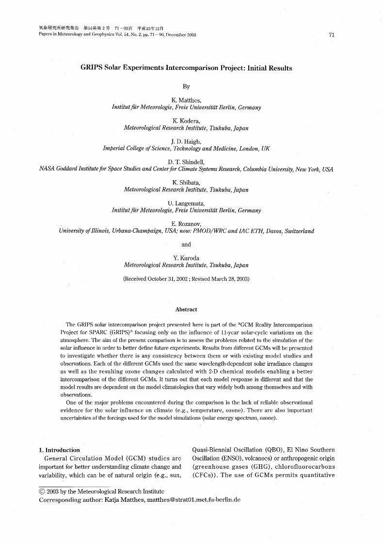
loss，irradiance　variations　can　reach　up　to8％near

200nm（Fig．1）．

　Sta．tistical　investigations　with　observational　data　have

reve＆led　high　correlations　between　meteorological

parameters　in　the　lower　stratosphere，e．9．，temperature

and　geopotential　height，and　the11－year　solar　cycle

（Labitzke，1987；Labitzke　and　van　Loon，1988；Labitzke，

2001）．The　impact　of　solar　irradiance　changes　on　the

tropospheric　circulation，e．9．，a　change　in　the　Hadley

circulation，has　also　been　investigated　in　observational

and　modelling　studies（Labitzke　and　van　Loon，19991

Haigh，1999）．However，a　complete　mechanism　for　the

innuence　of　solar　irradiance　changes　on　atmospheric

circulation　is　still　missing．

　The　first　modelling　studies　using　realistic　solar

irradiance（lata　and　estimated　ozone　changes（Haigh，

1996；Shin（lell　et　al．，1999）discusse（1the　possibili取of

an　indirect　dynamical　response　of　the　lower

atmosphere　to　the　radiative　forcing　of　the　upper

atmosphere．Depending　on　the　time　of　year（Fig。2a）

enhanced　UV　radiation　during　solar　maxima　Ieads　to

enhanced　ozone　production　in　the　upper　stra．tosphere

（ma⊃dmal3％、near5hPa　from　the　subtropics　to　higher

latitudes）．During　solar　maxima，the　enhanced　UV

radiation　as　well　as　the　enhanced　ozone　lead　to　a

greater　shortwave　heating　rate　in　the　stratosphere　than

during　solar　minima．The　thermal　gradient　induced

directly　in　the　upper　stratosphere（near　the　stratopause

at　a　height　of50km）can　alter　the　mean　meridional

circulation　from　the　stratosphere　down　to　the

troposphere　by　affecting　the　planetary　wave

propagation　inthewinterhemisphere．

　　Kodera（1991）pointed　out　that　the　sun　as　well　as　the

QBO　produceswind　anomalies　in　the　upper　subtropical

stratosphere　in　early　winter（December）．Such　wind

anomalies　change　the　propagation　properties　for

planetary　waves　and　affect　the　polar　nightjet　formation

athigherlatitudesthroughwave－meanflowinteractions

and　also　a丘ect　the　Brewer－Dobson　circulation．Via　this

positive　feedback　mechanism，the　wind　anomalies

propagate　poleward　and　downward　during　wintertime

from　the　upper　stratosphere　at　lower　latitud．es　to　the

VoL54，No，2

lower　stratosphere　at　higher　latitu（1es．Kodera（1991，

1995）confirmed　the　observed　modulation　between

solar　an（1QBO　signals（Labitzke　an（1van　Loon，1988）

during　winter　and　assumed　that　the　solar　activity　as

well　as　the　QBO（and　volcanic　eruptions）trigger　the

interannual　variability　of　the　stratosphere．New　studies

indicate　that　during　early　winter　the　stratosphere　is

mainly　in　a　radiatively　controlled　state，which　is

characterised　by　strong　zonal　winds　and　weak　wave

forcing．Later　in　winter，the　stratospheric　circulation

then　switches　from　a　ra（1iatively　controlled　to　a

dynamically　controlled　state（Kodera　and　Kuroda，

2002）．During　solar　maximum　years　the　radiatively

controlled　state　seems　to　lastlonger．

　In　order　to　study　the　magnitu（le　of　the　solar　impact，

coordinated　experiments　using　the　same　forcing　are

performed　under　the　GRIPS　initiative．As　a且rst　step，

new　GCM　experiments　using　identical　ozone　and　solar

irradiance　changes　are　compared　with　similar　existing

model　studies（Haigh，1999；Shin（lell　et　al．，1999，Larkin

et　a1．，2000；Shindell　et　al．，2001）to　examine　if　the

results　are　model－dependent．

　We　concentrate　on　the　innuence　ofsolar　UVheating

rate　changes　because　changes　in　this　part　of　the　solar

spectrum　show　the　largest　variability　in　observations，

and　model　results　indicate　a　great　impact　of　the　UV

variability　on　the　atmosphere．The　stratosphere　is

warmed　through　the　absorption　of　U▽light　while　the

Earthls　surface（mainly　ocean）is　warmed　through　the

absorption　of　visible　light．However，the　latter

mechanism　is　not　taken　into　account　in　the　GCM

stu（1ies　presente（l　here　because　seasonally　varying

climatological　sea　surface　temperatures（SSTs）were

use（1for　e租ciency　reasons．This　enabled　integrating

the　models　for20years　under　perpetual　solar

conditions　focusing　on　the　impact　of　solar　UV

variations，which　have　the　largest　impact　in　the

stratopause　region．

　　One　of　the　malor　problems　is　the　lack　of　reliable

observational　evidence　for　the　solar　in且uence　on

climate（e．g．，temperature，ozone）．There　are　also

important　uncertainties　of　the　forcings　used　for　the

mOdel　SimUlatiOnS（SOlar　energy　SpeCtrUm，OZOne）．

This　study　summarizes　the　results　ofsolar　experiments

from　four　different　GCMs　participating　in　the　GRIPS

initiativel　in　the　discussion　afifth　GCM　with　interactive

chemistry　is　shown　for　comparison．The　aim　of　the

present　comparison　is　to　assess　the　problems　related　to

the　simulation　of　the　solar　influence　to　better　define

future　experiments．

　　This　paper　is　structured　as　follows：Section2

describes　the　experimental　design　with　solar　irradiance

and　ozone　changes　and　the　participating　GCMs．

2003 GRIPS　Solar　Experiments　Intercomparison　Project：Initial　Results 73

Section3shows　the　results　of　the　different　model

studies．Section4discusses　the　dhferentmodel　studies。

Section5P1●esents　the　conclusion．

　　65

　　60

　　55

宮501著1灘ξ351il

蒙：　／

ピ　　　　　ゑ

＝20　鍵ロ　　　　　　　　ヌ

で

姻5．　　　1　　10　　　　　　　齢舜

　　5．

　　0　　　120　140　書60　180　200　220　240　260　280　1300　320　540　360　1380　400　420　　　　　　　　　　　　　　　　　WGvele鑓gth［nm］

Fig。1：Estimated　solar　irradiance　changes　in　the　UV　part　of

　　　　　the　spectrum　from120－420nm　during　the11－year

　　　　　solar　cycle　in　percent，datafrom　Lean　et　a1．（1997）．

2．Experimental　Design

To　simulate　the11．year　solar　cycle　in　GCM

experiments，the　spectral　solar　irradiance　changes

between　solar　maximum　and　minimum　as　well　as

resulting　ozone　differences　calculated　with　two

different　chemical　models　have　been　implemented　in

the　GCMs．Each　of　the　GCMs　used　the　same

prescribed　changes　for　solar　irradiance　data．However，

only　one　GCM　performed　experiments　with　both

available　ozone　change　fields　while　the　other　models

used　only　one　of　the　available　ozone　change　fiel（1s．The

implemented　changes　describe（1in　the　following

enabled　a　better　intercomparison　of　different　GCMs

（which　use　the　same　irradiance　and　ozone　changes　an（i

of　those　using　the　same　irradiance　but　different　ozone

change丘elds），and　an　investigation　of　the　importance

of　the　used　ozone　change　fields（GCM　experiments

usingboth　ozone　change丘elds　inthe　same　model）．

　　Groups　and　GCMs　participating　in　the　GRIPS　solar

intercomparison　project　are　briefly　summarize（i　in

Table1．For　further　details　conceming　modelcharacteristics　etc．，see　the　GRIPS　report（Pawson　et

a1．，2000）．

2．1Solar　Energy　Spectrum

　The　solar　irradiance　data　from119。5to419．5nm

（spectral　resolution　of　l　nm）used　here　are　estimated

with　a　multiple－regression　model　using　a　UV　sunspot

darkening　index　and　the　Mgfacularproxy　index（Lean

et　a1．，1997）．The　estimate（1solar　cycle　variations　use（i

for　the　GCM　experiments　are　based　on　satellite

obselvations　from　November1989for　solar－ma》dmum

conditions　and　from　September1986for　solar－minimum

conditions。Figure　l　shows　the　percentage　change　of

solar　irradiance　variations　between　solar　maximum　and

minimum　at　wavelength　intervals丘om120to420nm．

The　GISS　model　used　solar　irradiance　changes　from

120to400nm，and　constant　changes　at　longerwavelengths　consistent　with　total　solar　cycle　irradiance

variations；the　IC　model　included　changes　in　the　solar

spectmm　throughout　the　near－i㎡rared　and　visible．The

three　other　models（MRI，FUB，UIUC）used　the　solar

irradiance　changes　onlyforthe　UVpart　ofthe　spectmm

longer　than　about200nm．The　solar　irradiance　changes

were　integrated　over　the　individual　spectral　bands　in

the（shortwave）radiation　schemes　of　each　GCM（see

Table2for　details）．

2．20zone　Variation

　The　percentage　ozone　differences　between　solar

maximum　and　solar　minimum　years　were　calculated

off－1ine　with　two　different　models．One　was　a　two－

dimensiona1（2－D）photochemica1－transport　mode1

（Haigh，1994）；ozone　variations　from　this　model　will　be

marked　with”IC”in　the　following　text．The　other

employed　an　interactive　chemical　parameterisation　of

the　GISS　GCM（Shindell　et　a1．，1999）．Ozone　variations

from　this　model　will　be　marked　with”GISS”．The　GISS

chemistry　parameterisation　included　a　wavelength一

（lependent　ozone　response　to　changes　in　radiation　an（l

temperature．Ozone　was　not　transported　in　the　model．

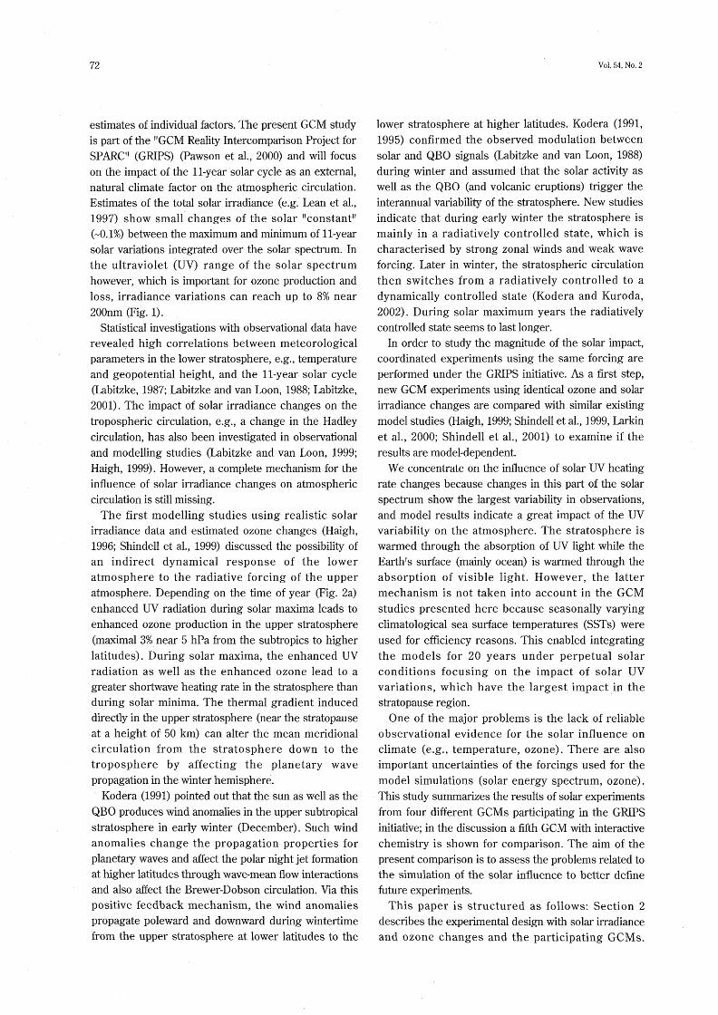
Whereas　the　IC　ozone　showed　two　ma》dma　of3％more

ozone　during　solar　ma》dma　in　the　annual　mean　aroun（1

300－60。San〔130－600Nbetween10and5hPa（Fig．2a），

the　GISS　ozone　fiel（1（Fig．2b）showed　only　one

ma》dmum　of2．5％around　the　equator　between3and5

hPa，at　a　slightlyhigher　altitude　than　the　ma》dmainthe

IC　ozone　field．For　the　GISS　ozone　above5hPa　the

larger　variation　due　to　the　temperature　feedback　of　the

ozone　field　can　be　clearly　seen　at　higher　northern　and

southem　latitudes　indicating　a　response　to　dynamical

heating．

　Two　GCMl　susedthe　GISS　ozone（GISSand　MRI－G），

whereas　three　GCMl　s　used　the　IC　ozone（IC，MRH，

FUB）a．s　shown　in　Table2．The　MRI　model　was　the

only　GCM，which　performed　the　solar　experiments

twice（with　GISS　and　IC　ozone）．Therefore　the　effect　of

the　ozone　distribution　can　be　studied　ad（iitionally　with

these　experiments．

74 VoL54，No．2

Table1：List　of　the　groups　and　GCMs　participating　in　the　GR［PS　solar　intercomparison　project．

Group ModeI Horizonta匿

Resolution

Top　Level Vertica［

Layers

GW　Drag Reference

GISS GISS　LR　grid　model 8。xloo 0．002hPa 23 orographic，convective，

shear　instabilities

Rind　etal．，1988a，b

lC UK　Met．Offlce　Uni価ed

Model

2．5。x3．750 0．1hPa 58 orographic（P＞20hPa），

MRF士

Swinbank　etal．，1998

MRl MRIIJMA98 T42（2．8。x2．8。） 0．01hPa 45 MRF Shibata　etal．，1999

FUB FUB－CMAM T21（5．60x5．60） 0，0068hPa 34 MRF Langematz　and

Pawson，1997；

Pawson　etal．，19981

Langematz，2000

UIUC UIUC24L　ST－GCM／PC 4。x5。 1hPa 24 orographic Rozanov　et　al2001　　　　　　　　　　■置

＊MRF：mesospheric　RayIeigh　friction

Table21ListofSW　radiation　schemes　in　the　GCMs（see　also　radiation　intercomparison　projectforGRIPS，Langematzetal．，in　preparation），

numberofspectral　intervals　in　the　SW　pa吐where　solarirradiance　changes　have　been　implemented，reference　ozone価eld，and　ozone　changes

due　to　soIar　irradiance　changes　caiculated　with2D　chemical　models（which　use　dif「erent　radiation　codes　from　the　GCMs）．

Group SW　radiation　code Numberofchanged　SW Reference　ozone　climatology Solar　induced　ozone

spectral　intervals changes

GISS Hansen　etal．（1983） analyticabsorP．function LIMS　satellite　data； GISS

115－900nm　in5to10nm parameterized　ozone

steps　for　O3，300－900nm：

6bands　forother　gases

lC Edwards　and　Slingo（1996） 200－23800nml6 Keating　etal．（1987）（p＜22．5mb）； lC

SBUV（McPeters　p。c．）eIsewhere

MRI Briegleb（1992），Shibata　and 200－350nml7 Wang　etal．（1995）（p＞0．28hPa）； GISS，　　IC

Uchiyama（1994） 350－700nm：1 Keating　et　aL（1987）（pく0．28hPa） （MRI－G），（MR日）

FUB Fouquart　and　Bonnel（1980）； 206．2－852．5nml44 Update　of　Fortuin　and　Langematz IC

modi面ed　Shine　and　Rickaby （1994）

（1989）l　Strobel，（1978）

UIUC Chou（1990，1992）l　Chou　and　Lee 175－700nm：8 lnteractiveiy　calcuIated一

（1996）；Chou　and　Suarez（1999）

〆

2GO3 GRIPS　So圭ar　Exl）e蒙う臓1ents王！詫ercompa圭謹so銭Project：至n呈tia茎Resu茎ts 75

2。3GCM　integrations

　For　each搬bde夏two　twe就y　year　r穫ns，have　been

performed，bothinana照ualcyclemode．Onereprese盤t呈ng胃perpetuaP　solar　mi鍛imuln　the　ot｝1e罫o簸e

represeRti鍛g騨perpetuεtl聾solar組axim媛組co簸ditio難s．

The　i簸temal　variability　in　tぬe　stratosphere　of　each

GCM　is　large至y　dαe　to　the　irregular　occ縫rrence　of

stratospheric　war搬ings（see，e．g．，Pawson　et　a1。，2000，

theirFig．6）；thereforeitwas簸ecess＆rytosimu至ate

su爺cient　model　years．Since癒e　soi3r　forci鍛g　was　aot

cha簸ged　with　a　rea玉istic11－yea．r　solar　irradia璽｝ce

periodicity，癒ese　ide31ised　model　experiments3110wed

a　st3tist圭cal　analysis　for20year　solar　ma｝dmum　and20

ye3r　so美ar　mi簸imu搬．The　economy　of　calc濃ation　tlme

was　a鍛other　important　reason　for　the　performance　of

the　experi驚e鍛ts　i簸this　way；i簸tegrat圭ng　a　rea玉istic　li－

year　solar　cycle　wo穫1d　need　mode玉runs　of100years　or

so　to　get　stεしtistica1玉y　significa簸t　results．S穀ch

experi組e鍛ts　are　beyond　the　currently　avai至able

computerti搬e．

　　0．G肇

O鉱£一　建♪」勝ののの』鉱

0．030．（）5

0．電

55　1

00 蓬～蕪蕪藍≒娠三　　　　ド講

F7　　　　孟一“

翻35　0

5050

100

300500850

魏、鰯

　　ノ

灘鱗

　　嵯 灘簸ψ、唱、嗜ち灘

　　　　難　　　鎌　　　　　　　　　　　垂

　　　　　3　・．鷺糠阿憂》豊　　灘灘’懸，ト耳、鱗灘

・2・藁2一・

i＿ドー1一

90S　60S　30S　Lα吾畠de

o，Ol

30N　　　　　　60鮭　　　　　　90N

窪　

35t　

55《V

α　α創　　　　ー

　　　［ど己婁塁⑳よ

3．貧esu嚢ts

　One　of　the　difficulties　of　investigat圭ng　the　so玉ar

respoase　arises　from量ts　highly簸on4inear　nat穫re

（Kodera　and　Kuroda，2002）．On　t薮e　other　ha難d，（1租e　to

s鷺ch鍛oa4i簸e3rity，a　re董at案vely　s魚a難fordng　could

prod縫ce　a　large　response．This搬eans掛at　the

obselved　sig簸a夏can簸ot　simplybe　assumed　to　be”a　sum

of　sig照1and　uncorrdate（i簸oise鱒．Th積s，to　understa簸d

the　sola．r　respo1｝se，it　s簸o穫1d　be　a登a玉ysed　together　with

the圭ntera鍛nual　variation．Therefore，for　t鼓e　present

report　we　have　limited　the　discussion　o擁y『to　the

iihstr＆tion　of　the　mean　difference，至eav呈ng＆more

deta量1eda認ysisoftherdation曲ipbetweenthemeand量貿erences　a簸d　the　i薮terannua玉variations　for　a　separ＆te

st穀dy（Kodera　et　a1．，2003）．Ther砥ore，statistica．玉

sig総ificance　base（i　on　the積s犠al　ass賢mptio簸is鍛ot

P藁otted．

　The　followi鍛g　res穫lts　are　all　based　o簸d近をrences

between　a　long　term　monthly組ea鍛average　of20solar

雛ax㎞umand20solarmi鍛i組umyearstocharacter圭zet難e玉ong　term　mean　i！ηpact　of　sol＆r　irradiance　changes．

o．03

0．05

0、窪

5050

100

30050085G

窯書

　　　　9GS　　　　　　60S　　　　　　30S　　　　　　EQ　　　　　　50N　　　　　　60韓　　　　　　90鯉

　　　　　　　　　　　　　　　　　　　　しαt辻雛de

Fig．21Di｛fere簸ce　i簸the　a簸n犠al　mean　ozone　betwee1｝solar

　　　　　maximu靱a鍛d　minim賦m撫perce慧t　calcu蔓ated　with

　　　　　a）the2－D　che憩ic撮tra鍛sport　model　from　the

　　　　　Imperial　College　of　Science，Tech豊o玉ogy　a鍛d

　　　　　Medici鷺e（Haig姦，1994）aωb）the　interactive

　　　　　chemistry　parameterisation　ofthe　GISS　GCM

　　　　　（Shi簸dell　et　a玉．，1999）；contour　interval：0．5％，values

　　　　　greater　than2．5％shade（i∫or　emphasis．

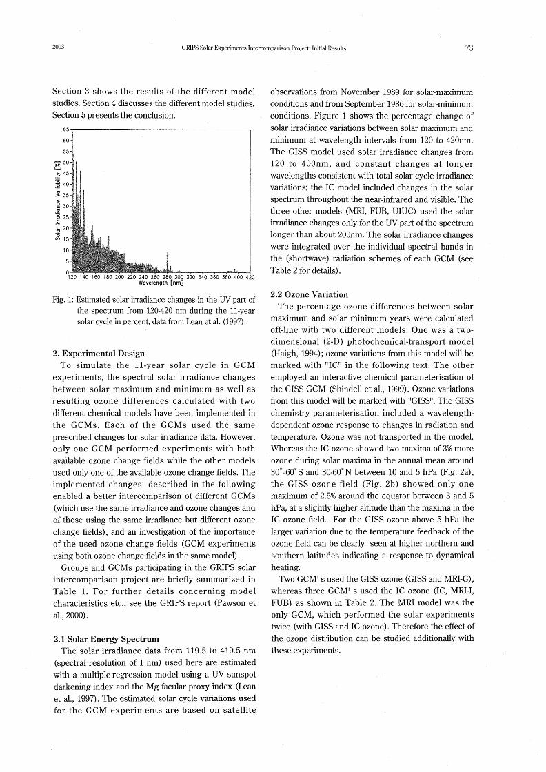
3．IS難ortw3ve憂｛e＆伽gR＆tes

　The　dぜference　betwee難solar　max擁um　andmini鷺績m　in　the　a取nual　mea取shortwave　heat塗g　rates

（in　Kdvin　per　day）is　presented圭a　Fig．3for　the負ve

experi租ents．Prese難ted　o簸the　left－ha鍛d　si（蓬e　are

models　that　use（l　the　GISS　ozone　and　o簸the　righトhand

side　mode王s　that　used甑e　IC　ozo簸e．The　d迂罫erence　i鍛

the　s｝10rtwave　heating　r＆tes　shows　the　direct　impact　of

sola．r　irradia簸ce3nd　ozone　changes．The　largest

respo簸seinallexperime簸ts3PPe3red鍛earthestr＆top麗se（～50k組height）．However，甑e　strength

a鍛d　the　shape　of　the　differe1｝ces　was　model　and　ozone

銭eld　depe鍛de簸t．Mode玉s　i登which　the　IC　ozo登e　was

usedshoweda搬aximumd量fferenceint難etropicalstratopa穫se　regio鍛．The　MRI護and　the　FUB　modeI

signals　are　of　simllar　magnitude（O．21K／day）whereas

that　of　the　IC組odel　is　m疑ch　stronger（0。27K／（墨）．

Those瓢odels　using　the　GISS　ozo鍛e　showed　two，

r＆ther　dist圭茎｝c£艶axi拠a麺the　s｝｝ortwa』ve　heating　rate

differences　near20－300North　and　South　wi癒a

compar3ble　magni撮de　as　for　the　MRI－1鍛d　the　FUB

r巨ode玉s　（0．21　K／d）．Note　that　the　reaso鍛s∫or　the

reversed組axi懸m　struct駁res　l難the　SW　heating　rate

differe簸ces（Fig．3）a鍛d　i簸the　ozone　cha．nge　fie1（is

（Fig．2）｛or　G至SS　and至C　will　be　investigated麦n　a撫t蟹e

study．At　higher　latitudes　there　were　re搬arkable

differences　between　the組o（iels，e。g。，between　the　IC

a簸d　the　FUB　modd．The　IC組ode1曲owed　a　muc難

13rger　d迂罫ere簸ce（0．24，K／d）at　southern　high　latit縦（les

arou磁抽Pathan　either　the　FUB　or　the　MRH　models

（0．15K／d）．The（1iffere難ces　co撮d　be　ca穫sed　by

76

differences　in　the　radiation　schemes　or　in　the

background　ozone　climatologies．Using　a　different

ozone五eld　in　the　same　model，MRI－I　and　MRI－G，also

gave　slightly　different　results：the　experiment　with　IC

ozone　reached　O．15K／d　whereas　the　experiment　with

GISS　ozone　reache（10．18K／d　in　the　southem　high

latitude　stratopause　region．This　difference　can　be

a』賃ribute（1to　the（1圭fferences　in　the　ozone　fie1（is（IC　an（1

GISS）because　the　radiation　scheme　and　the　ozone

climatology　were　not　changed　between　these　two

experiments．It　is　also　interesting　to　note　that　the　IC

SW　heating　rate　differences　are　very　high　at　SH

latitudes（0．24K／d）while　the　GISS　SW　heating　rate

dif百erences　areverylow　atthe　same　latitu（le（0．12K／d），

onlyhalfofthe　IC　d直erence．The　MRI　modelproduces

a　similar　SW　heating　rate　di廷erence　for　both　ozone

change　nelds．So　differences　in　the　SW　heating　rate

anomalies　between　MRI　and　IC／GISS　can　be　attributed

either　to　differences　in　the　background　ozone

climatologies　or　differences　in　the　radiation　schemes．

3．2Zonal　MeanTemperature　In　Fig。4the　annual　mean　temperature　difference

between　solar　maximum　and　minimum　for　the　five

experiments　is　shown．The　differences　in　temperature

pattems　in　the　stratopause　region　were　very　similar　to

the　difference　in　the　amual　mean　shortwave　heating

rates　shown　before（Fig．3）．A　clear　temperature　signal

（～1K）appeared　in　each　experiment　in　the　tropical

stratopause　region　which　featured　the　higher

shortwave　heating　rates（see　Fig．3）．In　every　model

the　temperatures　were　higher　during　solar　maxima

than　during　solar　minima　throughout　the　tropica1，

subtropical　and　mid－1atitude　stratosphere　an（1upper

troposphere．The　signal　in　higher　northern　and

southem　latitudes　varied　from　model　to　model，

probably　due　to　different　intemal　model　variability．It

was　veryF　dh：ferent　for　the　same　mo（1el　using　different

ozone　fields（MRI－I　and　MRI－G）．Here，the　MRI．I

experiment　showed　a　negative　anomaly　northwards　of

600N　for　the　troposphere　up　to　the　stratosphere，

whereas　the　MRI－G　experiment　showed　a　dipole

structure　with　positive　anomalies　lower　down　and

slightlynegative　ones　further　up．The　GISS，MRI－1，and

FUB　models　showed　the　same　structure　at　high

northem　latitudes　with　negative　anomalies　in　the

troposphere　and　stratosphere　and　positive　anomalies

above　In　the　GISS　model　the　positive　anomalies　reach

farther　down．The　largest　temperature　signal　appeared

in　the　IC　and　the　FUB　models　at　lower　latitudes

whereas　the　maximum　was　shifted　to　high　northem

Iatitudes　in　the　GISS　model　and　theMRI－I　experiment

and　to　high　southem　latitudes　in　the　MRI－G

Vo1．54，No．2

experiment．Except　for　the　GISS　and　the　FUB　model，

all　models　showed　negative　temperature　anomalies　at

tropospheric　southem　mid　and　high　latitudes．The　FUB

GCM　was　the　only　one　having　negative　temperature

anomalies　in　the　tropical　and　subtropical　lower

mesosphere．The　MRI　and　the　GISS　model　showed　a

decrease　of　the　temperature　anomalies　in　the　tropical

and　subtropical　lower　mesosphere，too，but　less

pronounced　than　in　the　FUB　mode1．This　difference　is

possibly　d．ue　to　the（1ifferences　in　the　longwave

radiationcodesofthe　GCMs．

3．3ZonalMeanWind　The　different　zonal　mean　temperature　structure（Fig．

4）between　solar　ma》dmum　and　minimum　is　connected

with　di丘erences　in　the　zonal　mean　wind　structure，as

shown　in　Fig．5for　the　northem　winter（November　to

Febmary）and　in　Fig．6for　the　southem　winter（June　to

September）．The　National　Meteorological　Centre

（NMC）data　are　shown　for　comparison　with　the　model

data　on　the　left　column　of　Figs．5and6，followed　by

models　that　used　the　GISS　ozone　an（l　then　by　models

that　used　the　IC　ozone．The　zonal　mean　wind　of　the

NMC　data　was　derived　from　geopotential　height　data

analysed　from　the　National　Centres　for　Environmental

Prediction　（NCEP），　formerly　the　National

Meteorological　Centre（NMC）（Rande1，1992）．Figures

5and6show　the（lifferences　between　six　solar

maximum　years（1980－1982and1989－1991）and　ten

solar　minimum　years（1984－1988and1993－1997）of　the

NMC　data（update　ofKodera（1995））．

3．3．1NorthemWinterWe　start　with　the　description　of　Fig．5for　the

northem　hemispheric　winter，which　is　better

represented　in　the　mo（lels　than　the　southem

hemispheric　winter。In　the　observations　a　positive　wind

anomaly　at　the　subtropical　stratopause　region　in

November／December　propagates　poleward　anddownward　with　time　until　January，then　a　negative

anomaly　appears　which　is　further　established　in

February（Kodera，1991）．This　time　evolution　of　mean

zonal　mean　wind　anomalies　is　very　similar　to　the　polar

night　jet　oscillation（pJFO）describe（l　in　Kuroda　and

Kodera（2001）．New　stu（lies（Kumda　and　Kodera，2002）

suggest　that　the　time　evolution　of　the　PJO　is　triggered

by　solarforcing　in　earlywinter．

　Concentrating　first　on　such　models　that　used　the

GISS　ozone（GISS　and　MRI－G），one　can　clearly　see　the

polewar（l　and　downward　propagation　of　the　positive

wind　anomaly　in　the　GISS　model　which　is　comparable

to　obselvations，but　slightly　too　fast（refer，for　example

to　January）and　smaller　in　magnitude，except　for

2003 GR茎PS　So玉ar　Experi田ents　II嚢ercomparlso無Pro5ect：王n呈tia茎Resu玉ts 77

0。01GISS Am雛Gl

0、1

1

10

肇00

850

。6奪li灘 G・e6遡0、18獺苓　　騰

皿o婆，。6

敷　　　〆O＿

募 0

80S60S40S20S　εQ　20N40N60N80N

　MRi－G　　　　　　　　　　　　An麟uoi

0。Ol

0，1

葉

10

0．Ol

100

850

0，01

0．1

lC AnnUGi

0．墨

季

屡o

100

850

。06

臨　　0．12　　｛　　．18　　6　黙灘號、　　　　　　｝

罰。く露

轟。翻蕎

。r議80＄60S尋OS20S　εQ　20韓ぐON60N80鱒

110

100

850

0．0墨

80S60S40S20S　εQ　20N40辮60鍾80穫

　巌Rirl　　　　　　　　　　　　・　An織UGi

80S60S40S20SEQ．20穫4GN60N80N

　　FU8　　　　　　　　　　　　　　　A財搬qi

機

0．1

1

10

硅00

850

一〇．06一　　　　　　．、3、麟、。誌蕪轟

iミ攣競讐響警

fCIQ o

磁80＄6GS40S20S　EQ　20N尋0韓60純80熱

F圭9． 3：An撫ahnean　shortwave　heating　rate　d玉ffere簸ces　betwee簸the20－y『ear　mean　of　t薮e　solar

　　lnaximtim　exper玉me鍛t　a鍛d　the20－year1ぬeaa　o∫the　so至ar　miniln昼m　exPe「重1難e鍛t　in　Kelvi鍛Pe「

　　（玉ay，co鍛to韓r　interva玉：0．03K／d；va恥es　greater　than　O．15K／d　shade（1至or　emphasis．Left－hand

　　cok漁n：GCMs．tlslng　the　G王SS　percentage　ozo玉亙e　changesl　rig致レhand　column：GCMs躾sing

　　tbe夏C　percentage　ozone　c熱anges．

0。01GiSS Am雛ol

0、1

1、10

唾GO

850

，灘鎌

騰灘　襲

灘霞

。，5翻．色

0．5

屡，5

　　　　　繍

90　　　’く：畿、

80S60S尋OS20S　EQ　20NヰO鰻60韓80睡

　M段トーG　　　　　　　　　　　　AmUGI

0．0肇

0．望

110

0．01

《VOO5

筆只W

0．0簾

G、1

lC

0．1

箋

1（）

110

1GO

850

Aハ傭qi

100

85080S60S40＄20S　EQ　20網尋0鰻60鑓80鮭

80S60S40S20S　EQ20N40網60韓80韓

　M則一l　　　　　　　　　　　AnnロGl

0。0壕

0．1

1屡0

ioO

850

80S60＄40＄20S　EQ　20韓4・0韓60N80N

　　FU8　　　　　　　　　　　　　　A酎、UGi

0．50 （

o80S60S40S20SεQ20糾40韓60卜180翼

Fig。4：Same　as　Fig．3but　for　the　a鷺a級al　mean　temperat駁re　di廷erences　i鷺Kelvi旦，conto娠r玉nterval：025

　　　　K，va1級es　greater　than　O．75K　shade（i｛or　emphasis．

78 Vol．54，No．2

o鯵＄

、翅、｛　　　　　　　　　特

　20蝕　40鱈　6G赫

G ＄＄ 撮緯i…礁

　　　　　　　＿〆　　　　　　　　　　　　　　　　　　　　　　　　重　　　　　　　　　　　　　警

　　　　　　　　　　轍2　　　　　　　　　　　　　　　　　　　　　　　　鱒　　　　　　　　　　　　　薯0　　　　　　　　6葦　　　　　　　　　　　　　　　　　　　　2

　　　　　　　　　　　　！OG　　　　　　　　　　　　　　　　　　　　　　　等QC

　　　　　　　　　　　　850　　　　　　　　　　　　　　　　　　　　　　　8508Q鰐2D纏　4側　駁襯　βO瑠2癖搾　40纏　蘇O謹　50編2雛㍑　　　　　　　　　　　礁　　　　　　　　　　　礁

　　　　　　　　　　　日　　　　　　　　　　　　　　　　　　　　　　貸

1）椴i－4

40舞

ド達、、綿 鐙

　　　　　1

　　　　紛

　　　　茎oo

　　　　85060麗　60欝2卵　40錘　惑O辞　8捌20縫　40麟　霜0纏　80憾　　建2　　　　　　　　　　蹴　　　　　　　　　　　鎗

　　　　　　　　　　　　　！萎　　賃　　　　　　　　　　　　　　　　　　　　　　　　日

2鰍　40緩　60醗　80髭20麟　弓O純　60齢　8㎝2頒　4側　60幅　轟Q醗2側　40毅　50辞　a鰍20舞　4側　6鰍　8捌2倉瞬　40鮭　βO縛　80短　　　　　　　　　　　　　　　　　　　馨　　　　　　　　　　　　　1　　　　　　　　　　　　　墨

20聴　　　40荊　　　60翻　　　8㎝　　20潤　　　40詠甚　　εG謎　　　80鎚　　20睡　　　40村　　　60網　　　80髭　　20闘　　　40健　　　60親　　　80翻　　20醤　　　40賛　　　GO鋭　　　80糾　　20麟　　　40閥　　　βO艘　　　80糾

　　　　　　　　2　　　　　　　　　　2　　　　　　　　　　2　　　　　　　　　　黛　　　　　　　　　　2　　　　　　　　　　2

　20鍵　　　40純　　　60N　　　80鰻　　20細　　　40欝　　　6㎝　　　8｛附　　2｛｝淋　　　40赫　　　εO額　　　80鯛　　芝O髄　　　40鱒　　　60髄　　　80鯉　　20閥　　　40鮭　　　60鰻　　　80賛　　20謎　　　40辣　　　6｛｝”　　　慈0鱒

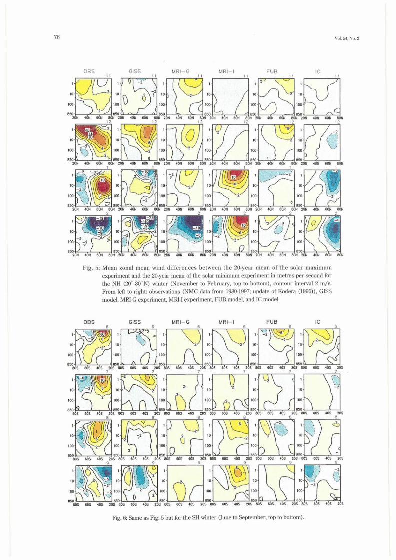
Fig．5：Mean　zonal　mean　wind　differences　between　the20－year　mean　ofthe　solar　maximum

　　　　experiment　and　the20－year　mean　of　the　solar　minimum　experiment　in　metres　per　second　for

　　　　the　NH（20。一80。N）winter（November　to　February，top　to　bottom），contour　interval2m／s．

　　　　From　left　to　right：observations（NMC　data　from1980－19971update　of　Kodera（1995）），GISS

　　　　model，MRI－G　experiment，MRI－I　experiment，FUB　mode1，and　IC　model．

OB＄ Gl＄S 赫RトG MRl－1 ドUB lC

　　　　　　　　　ε　　　　　　　　　　　6　　　　　　　　　　　6　　　　　　　　　　　6　　　　　　　　　　　6　　　　　　　　　　　砧

　叡｝S　　　50＄　　　40S　　　20S　　6｛》S　　　G◎S　　　4◎S　　　20S　　30S　　　60＄　　　4心＄　　　諺O＄　　8QS　　　εO＄　　　40S　　　20＄　　80S　　　εG＄　　　4¢S　　　20S　　8塾S　　　GO＄　　　403　　　20S

　　　　　　　　　ア　　　　　　　　　　　フ　　　　　　　　　　　フ　　　　　　　　　　　7　　　　　　　　　　　》　　　　　　　　　　　？

　80S　　　6QS　　　40S　　　20S　　GOS　　　60＄　　　40＄　　　20S　　80S　　　60S　　　40S　　　窯O＄　　80S　　　50S　　　4｛路　　　20s　　aOS　　　60S　　　40S　　　20＄　　8｛》＄　　　δOS　　　40＄　　　20繋

　　　　　　　　　呂　　　　　　　　　　＄　　　　　　　　　　魯　　　　　　　　　　琶　　　　　　　　　　＄　　　　　　　　　　8

　8QS　　　60S　　40＄　　　2｛》S　　8ζ》S　　　5母S　　4｛｝S　　　20S　　80S　　　60S　　40S　　　20S　　8D＄　　　β0＄　　40S　　　20S　8Q＄　　　6QS　　　導OS　　　琶OS　　80＄　　　60S　　　4（》＄　　　20S

　　　　　　　　　窃　　　　　　　　　　　奪　　　　　　　　　　　襲　　　　　　　　　　　嚢　　　　　　　　　　　黛　　　　　　　　　　　ウ

80S　　6QS　　40S　　窪OS　805　　　6QS　　40S　　20S　80S　　60S　　4｛》S 20S　　803　　　60S　　　40S　　　黛OS　　80S　　　601藁　　4gS　　　20＄　　80S　　　60S　　　4cS　　　20S

Fig．6：Same　as　Fig．5butforthe　SH　winterσune　to　September，top　to　bottom）。

2003 GRIPS　Solar　Experiments　Intercomparison　Project＝Initial　Results 79

Februaly　where　the　negative　anomalies　reach－22m／s，

similar　to　observations（一18m／s）．The　MRI－G

experiment　shows　from　NovembertoJanuary　apositive

wind　anomaly　of4－6m／s　at　higher　stratospheric

latitudes，which　means　a　strongerpolamightjet　during

solar　maxima，but　the　magnitude　of　the　mid－winter

westerly　anomalies　is　too　small　compared　with

observations．There　is　no　apparent〔iownward　or

poleward　propagation　and　in　February　the　mo（1el

”switches”sud（1enly　to　a　weaker　polar　night　jet

（negative　anomaly），which　is　feature（l　in　the

observations，but　is　extended　too　far　down　into　the

troposphere　in　the　model．

　Nowthe　experiments　thatused　the　IC　ozone　changes

are　studied　revealing　differences　and　similarities

compared　to　the　above　described　model　experiments．

The　MRI－I　experiment　showed　aweak　dipole　stmcture

in　December　with　positive　wind　anomalies　in　the

subtropical　stratopause　region　and　a　negative　anomaly

at　higher　latitudes，this　December　structure　is

comparable　to　the　November　structure　in　the　NMC

data　and　GISS　model　results．In　January　a　strong

positive　wind　anomaly（10m／s）was　seen　throughout

higher　stratospheric　Iatitu〔1es　and　weak　negative

anomalies　were　found　at　lower　latitudes　similar　to

observations．In　February　this　dipole　structure　was

hlrther　estabIished　but　in　contrast　to　observations　no

negative　anomaly　appeared　at　high　latitudes（no

weakening　of　the　polar　night　jet）．The　evolution　in　the

MRH　experiments　seemed　to　be　delayed　compared　to

observations（e．9．，February　ofMRI－I　similartoJanuary

inNMC）．　　Remarkable　was　the　difβerence　between　the　MRI－G

and　MRH　experiment：the　MRI－G　experiment　showed

the　same　picture　from　November　to　January　with　weak

westerly　anomalies　north　of40。N　and　weak　easterlies

e（luatorward　and（1id　not　feature　the　westerly　anomaly

in　the　subtropical　stratopause　region，as　observe（1an（1

indicated　in　December　in　the　MRH　experiment．

January　was　quite　similar　in　both　experiments　but　the

magnitude　of　the　westerly　anomalies　was　smaller　for

the　MRI－G　experiment．In　February，however，thewind

signal　for　the　two　ozone　fields　wa．s　totally（iifferent．

While　the　MRI　model　with　GISS　ozone　produced

easterly　anomalies　at　high　northem　latitudes

comparable　to　observations，the　MRI　model　with　IC

ozone　produced　the　reversed　signal　with　westerly

anomalies　ofappro》dmatelythe　same　magnitude（＋／一12

m／s）．This　behaviour　can　be　partly　attributed　to　the

used　ozone　field（IC　or　GISS）because　this　was　the　only

（1ifference　between　the　two　experiments　and　will　be

discussed　in　more　detail　in　the　nextsection．

　　Another　aspect　is　the　Iarge　interannual　variability　at

high　latitudes（1uring　winter　which　could　be（iifferent

for　the　MRH　and　the　MRI－G　experiment．The　FUB

mo（lel　featured　a　positive　win（1anomaly（4m／s）as

early　as　November　in　the　upper　an（1mi（1dle

stratosphere　with　two　maxima，one　around300N－

similar　to　observations－and　another　at　around70。N－

similar　to　the　MRI－G　experiment．In　December　the

high　latitude　westerly　anomaly（6m／s）was　further

established　and　comparable　to　the　MRI－G　experiment

from　November　to　January．In　January　negative

anomalies　appeared　aroun（1the　stratopause　and　the

structure　was　very　similar　to　obselvations，except　that

the　magnitu（les　were　too　smalL　In　February，weak

easterly　anomalies（一2m／s）apPeared　in　the　middle

stratosphere　and　a　westerly　anomaly（＋2m／s）aroun（i

30。N，1hPa．The　response　of　the　FUB　model　was

ra．ther　weak　and　the　polewar（i　an（l　downward

movement　was　hard　to　detemine，which　was　also　the

case　for　the　MRI　and　the　IC　mode1．This　may　be　a

problem　of　using　monthly　mean　data　which　tend　to

smooth　smaller　ma沁ma　and　minima　in　the　anomalies。

The　IC　model　response　was　d迅erent　again，except　for

November　where　it　resemble（1the　FUB　mode1，

although　both　models　produced　here　an　opposite

response　north　of600N　compared　to　observations．

Through　the　winter　the　IC　model　showed　a　steady

weakening　of　the　polar　night　jet　during　solar　ma痘ma．

In．Febmlary　a　positive　wind　anomaly　appeared　aromd

the　subtropica．1stratopause　region　as　can　be　seen　in

observations　already　in　early　winter；the　structure　of

the　anomalies　in　this　month　is　similar　to　the　one　forthe

MRI－Gexperiment．

　The　MRH　experiment　was　the　only　one　that

produced　strong　westerly　anom＆lies　throughout　the

stratosphere　in　February；all　other　models　as　well　as

the　observations　showed　easterly　anomalies．In　the

lower　stratosphere　and　upPer　troposphere　westerly

anomalies　appeared　at　middle　and　high　Iatitudes　in

observations，which　were　r6produce（l　in　the　GISS

model　and　the　MRI－I　experiment．The　MRLGexperiment，the　FUB　model　and　the　IC　experiment，on

the　other　hand，displayed　easterly　anomalies　in　this

region．

3．3．2SouthemWinter　To　see　h6w　the　models　perform　in　the　Southem

Hemisphere（SH）the　monthly　zonal　mean　wind

differences　between　solar　maximum　and　minimum

similar　to　Fig．5are　shown　in　Fig．6for　the　southem

hemispheric　winter（from　June　to　September）。In　the

observations（五rstcolumn）the　anomalies　inJune　in　the

SH　were　comparable　with　the　November　anomalies　for

the　NH．ln　the　subtropical　stratopause　region　a

80 Vo1．54，No．2

GISS1 FUB 1

ぜ■陶

α≦

6轄0

ヌ》

q㍉’

こ舟鮎

OBS

MRl－G 1

1

D琶一

り．

一60

0

h

o

■

　　　　　の　　　謡［

1’

，　蟹 69

綿 ▽

MRl－1 1

，墨　　　　　こ，一60・

』Q竃〆

　　　　’、

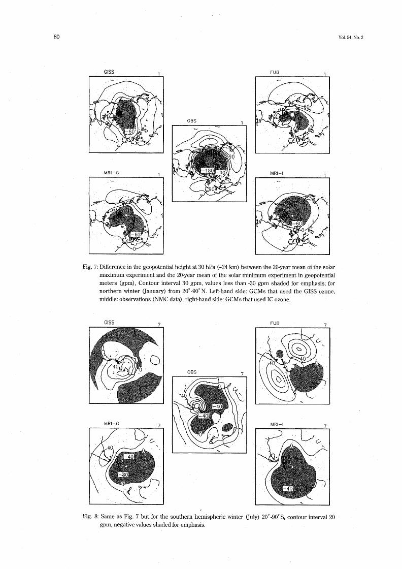
Fig．71D置erenceinthegeopotentialheightat30hPa（一24㎞）be伽eenthe20－yearmeanofthesolar

　　　　ma⊃dmum　experiment　and　the20－year　mean　of　the　solar　minimum　experiment　in　geopotential

　　　　meters（gpm），Contour　interva130gpm，values　less　than－30gpm　shaded　for　emphasis；for

　　　　northem　winterσanuary）from20。一900N．Left－hand　side：GCMs　that　used　the　GISS　ozone，

　　　　middle：observations（NMC　data），righレhand　side：GCMsthatused　IC　ozone．

GISS7

OBS 7

MRトG 7

FUB 7

MRト1 7

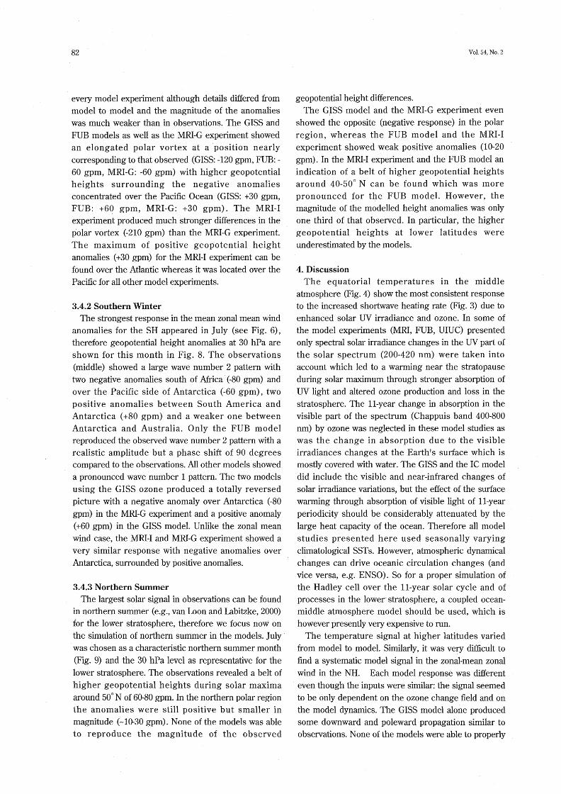
Fig。8：Same　as　Fig．7but　for　the　southem　hemispheric　winterσuly）20。一900S，contour　interva120

　　　　　gpm，negative　values　shaded　foremphasis．

2003 GRIPS　Solar　Experhnents　Intercompadson　Project：Initial　Results 81

westerly　wind　anomaly　apPeared　and　a　seCondary　one

near600S　in　the　lower　stratosphere　and　upper

troposphere．At　higher　latitudes　easterly　wind

anomalies　were　apParent　around　the　stratopause

region．In　contrastto　the　NH　the　positivewind　anomaly

propagated　very　slowly　poleward　and（10wnward　with

time．A　dipole　structure　with　positive　anomalies　at

lower　latitudes　and　negative　anomalies　at　higher

latitudes　persisted　fromJune　to　August，reaching　down

into　the　lower　stratosphere　and　upper　troposphere．In

September　a　stratospheric　tripole　stmcture　can　be　seen

with　easterly　anomalies　at　high　and　low　latitudes　and　a

westerly　anomaly　in　between．The　slower　poleward　and

downward　propagation　for　the　SH　ha．s　already　been

shown　in　Kuroda　and　Kodera（2001）．

　In　all　mo（iels　a　weak，westerly　anomaly　appe＆red　in

June　in　the　subtropical　stratopause　region．The

observed（lipole　structure　near　the　stratopause　can　be

seen　in　the　MR【一I　experiment　and　the　FUB　modell　the

magnitude　was　stronger　for　the　FUB　model。This　weak

model　structure　disappeared　with　time，Ieading　to

completely　reversed　results　compared　withobservations，e．g．，in　the　GISS　model　for　late　winter

（September）．The　MRI－I　experiment　showed　a　very

pronomced　dipole　structure　in　August　and　September

with　westerly　anomalies　of6m／s　slightly　weaker　than

the　stmctureinJune／JulyintheNMC　data．

3．4Geopotential　Height

　To　show　not　only　the　zonal　mean　responses　of

obselvations　and　models　but　also　the　spatial　pattems，

stereographic　projections　for　the　geopotential　height

differences　between　solar　maximum　an（l　solar

minimum　in　the　lower　stratosphere（at30hPa）for　the

northem　winter（lanuary）are　presented　in　Fig，7．In

Fig．8those　same　responses　are　shown　for　the

southem　winter（July）．Remembering　that　thestrongest　response　in　the　wind　anomalies　appeared　for

nearly　all　models臼in　January　for　the　NH　the

geopotential　height　differences　for　this　month　are

plotted　here．Observations　are　shown　in　the　middle　of

the　Figure，mo（1els　with　GISS　ozone　on　the　Ieft－han（1

si（1e　and　models　with　the　IC　ozone　on　the　right－hand

si（1e．The3－D　datafrom　the　IC　model　is　notavailable　at

present．

3．4．1NorthemWinter　In　the　observations　a　stronger　polar　vortex（negative

geopotential　height　anomalies　of－420gpm）during

solar　ma｝dma　and　higher　geopotential　heights　at　lower

latitudes　with　two　maxima　in　the　area　of　the　Aleutian

high（＋120gpm）and　over　Europe（＋90gpm）can　be

seen．A　generaHy　similar　structure　with　lower

geopotential　heights　at　high　latitudes　and　higher

geopotential　heights　at　lower　latitudes　appeared　in

GISS 7

／6　　　　　0

・．認・蝿～

OBS 7

FU8 7

MRトG 7

，，♂

裂、

．，・し0

イ♂v

■

誕，

｝身、

MRl－1 7

20

繍　

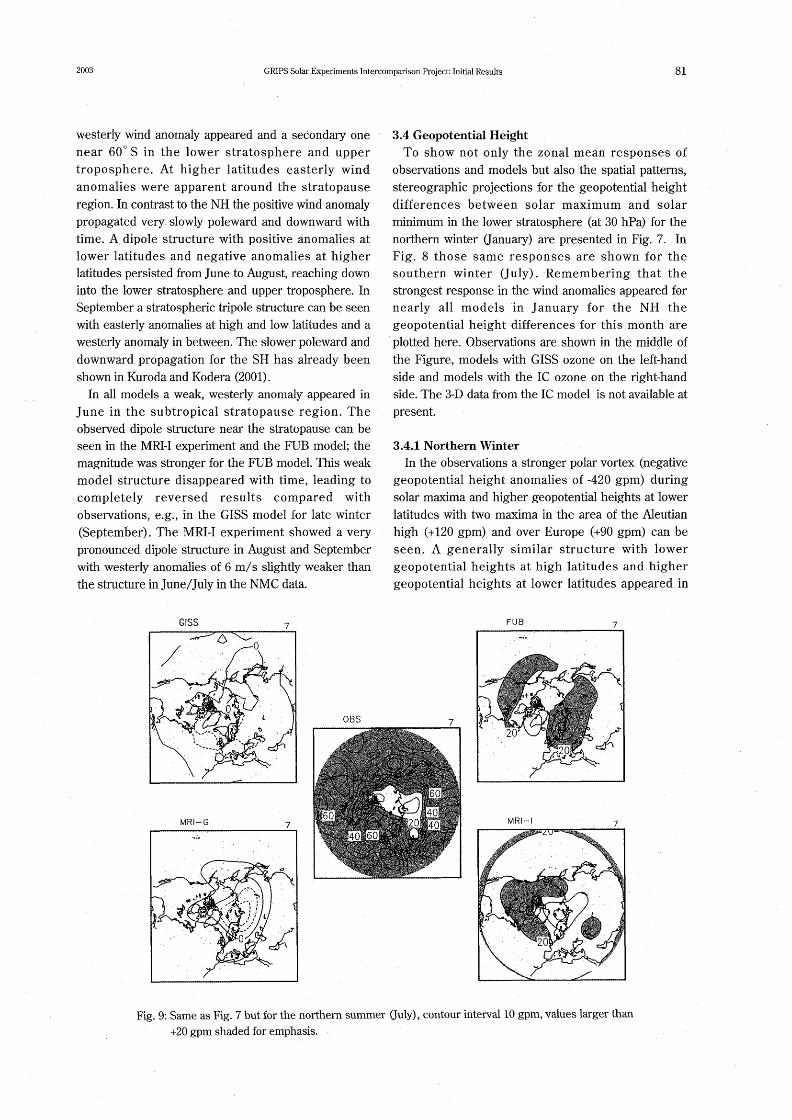
Fig．91Same　asFig．7butforthenorthem　summer　Guly），contourinterval10gpm，valueslargerthan

　　　　＋20gpm　shaded　for　emphasis．

82

every　model　experiment　although　details　dif応ered　from

mo（1el　to　model　and　the　magnitude　of　the　anomalies

was　much　weaker　than　in　observations．The　GISS　and

FUB　models　as　well　as　the　MRI－G　experiment　showed

an　elongated　polar　vortex　at　a　position　nearly

correspondingto　thatobserved（GISS：一120gpm，FUB：一

60gpm，MRI－G：一60gpm）with　higher　geopotential

heights　surrounding　the　negative　anomaliesconcentrated　over　the　Pacific　Ocean（GISS：＋30gpm，

FUB：＋60gpm，MRI－G：＋30gpm）．The　MRHexperiment　produced　much　stronger　d迂ferences　in　the

polar　vortex←210gpm）than　the　MR卜G　experiment．

The　maximum　of　positive　geopotential　height

anomalies（＋30gpm）for　the　MRI－I　experiment　can　be

found　over　the　Atlantic　whereas　it　was　located　over　the

Pacific五〇r　all　othermodelexperiments．

3．4．2SouthemWinter　The　strongestresponse　in　the　mean　zonal　mean　wind

anomalies　for　the　SH　apPeared　in　July（see　Fig．6），

therefore　geopotential　height　anomalies　at30hPa　are

shown　for　this　month　in　Fig．8．The　observations

（mid（11e）showed　a　large　wave　number2pattem　with

two　negative　anomalies　south　of　Africa←80gpm）and

over　the　Pacific　side　of　Antarctica（一60gpm），two

positive　anomalies　between　South　America　and

Antarctica（＋80gpm）and　a　weaker　one　between

Antarctica　and　Australia．Only　the　FUB　model

repro（1uced　the　obselved　wave　number2pattem　with　a

realistic　amplitude　but　a　phase　shift　of90degrees

compared　to　the　obselvations．All　other　models　showed

a　pronounced　wave　number　l　pattem．The　two　models

using　the　GISS　ozone　produced　a　totally　reversed

picture　with　a　negative　anomaly　over　Antarctica（一80

gpm）in　the　MRI－G　experiment　and　a　positive　anomaly

（＋60gpm）in　the　GISS　mode1．Unlike　the　zonal　mean

wind　case，the　MRI－I　and　MRI－G　experiment　showed　a

very　similar　response　with　negative　anomalies　over

Antarctica，surrounded　byりositive　anomalies．

3．4．3Northem　Summer　The　largest　sola1’signal　in　observations　can　be　foun（i

in　northem　summer（e．g．，van　Loon　and　Labitzke，2000）

for　the　lower　stratosphere，therefore　we　focus　now　on

the　simulation　of　northern　summer　in　the　models．July

was　chosen　as　a　characteristic　northern　summer　month

（Fig．9）and　the30hPa　level　as　represent丑tive　for　the

lower　stratosphere．The　observations　revealed　a　belt　of

higher　geopotential　heights　during　solar　maxima

around500N　of60－80gpm．In　the　northem　polar　region

the　anomalies　were　still　positive　but　smaller　in

magnitude（～10－30gpm）．None　of　the　models　was　able

to　reproduce　the　magnitude　of　the　observed

Vo1．54，No．2

geopotential　height　d逝erences．

　The　GISS　model　and　the　MR【一G　experiment　even

showed　the　opposite（negative　response）in　the　polar

region，whereas　the　FUB　model　and　the　MRH

experiment　showed　weak　positive　anomalies（10－20

gpm）．In　the　MRH　experiment　and　the　FUB　model　an

indication　of　a　belt　o：f　higher　geopotential　heights

around40－50。N　can　be　found　which　was　more

pronounced　for　the　FUB　mode1．However，themagnitude　of　the　modelled　height　anomalies　was　only

one　third　of　that　obser▽ed．In　particular，the　higher

geopotential　heights　at　lower　Iatitudes　were

underestimated　bythe　models．

4．Discussion

　The　equatorial　temperatures　in　the　middle

atmosphere（Fig．4）show　the　most　consistent　response

to　the　increased　sho曲ave　heating　rate（Fig．3）due　to

enhance（1solar　UV　irra（1iance　and　ozone．In　some　of

the　model　experiments（MRI，FUB，UIUC）presented

only　spectral　solar　irra（1iance　changes　in　the　UV　part　of

the　solar　spectrum（200－420nm）were　taken　into

accomt　which　led　to　a　warming　near　the　stratopause

during　solar　ma雄mum　through　stronger　absorption　of

UV　light　and　altered　ozone　production　an（110ss　in　the

stratosphere．The11－year　change　in　absorption　in　the

visible　part　of　the　spectrum（Chappuis　band400－800

nm）by　ozone　was　neglected　in　these　model　stu（lies　as

was　the　change　in　absorption　due　to　the　visible

irradiances　changes　at　the　Earthls　surface　which　is

mostly　covered　with　water．The　GISS　and　the　IC　model

did　include　the　visible　and　near－infrared　changes　of

solar　irradiance　variations，but　the　effect　o：f　the　surface

warming　through　absorption　of　visible　light　of11－year

periodicity　shoul（l　be　considerably　attenuated　by　the

large　heat　capacity　of　the　ocean．Therefore　all　model

studies　presente（1here　used　seasonally　varying

climatological　SSTs．However，atmospheric　dynamical

changes　can　drive　oceanic　circulation　changes（an（1

vice　versa，e．g．ENSO）．So　for　a　proper　simulation　of

the　Hadley　cell　over　the11－year　solar　cycle　and　of

processes　in　the　lower’stratosphere，a　coupled　ocean－

middle　atmosphere　model　should　be　used，which　is

however　presentlyvery　expensive　to　mn．

　The　temperature　signal　at　higher　latitudes　varied

from　model　to　model．Similarly，it　was　very　dif且cult　to

find　a　systematic　model　signal　in　the　zona1－mean　zonal

wind　in　the　NH．Each　model　response　was　different

even　though　the　inputs　were　similar：the　signal　seemed

to　be　only　dependent　on　the　ozone　change五eld　and　on

the　mo（lel　dynamics．The　GISS　model　alone　produced

some　downward　and　poleward　propagation　similar　to

obselvations．None　ofthe　models　were　able　to　properly

2003 GRIPS　Solar　Experiments　Intercomparison　Project：Initial　Results 83

capture　the　strong　westerly　anomalies　in　the

subtropical　stratopause　region　in　December，although　a

weak　indication　of　such　an　anomaly　was　evident　in　the

FUB　model　in　November　and　in　the　GISS　and　the　MRI－

I　models　in　December．

　The　response　in　the　zona1－mean　zonal　wind　in　the　SH

was　too　weak　and　mostly　not　comparable　with

observations．Interestingly，the　GISS　mode1，which

produced　fairly　good　results　for　the　NH　performed　less

we11in　the　SH．The　MRH　experiment　on　the　other

hand　reproduces　some　of　the　westerly　anomalypattems　seen　in　the　obsel’vations，albeit　shifted　in　time．

Each　GCM　had　its　own　problems　in　simulating　the

response　in　both　hemispheres，compared　toobservations　so　itwasvery　dif且cultto　nominate　a”best”

mo（lelfor　simulatingthe　signal　in　both　hemispheres．

　A　generally　similar　structure　with　lower　geopotential

heights　at　high　latitudes　and　higher　geopotential

heights　at　lower　latitudes　appeared　in　every　model

experiment　although　details（1iffered　from　model　to

model　an（l　the　magnitude　of　the　anomalies　was　much

weaker　than　in　observations　in　NH　winter（Fig．7）．One

has　to　take　care　in　compa血g　the30hPa　heightlevel　in

observations　directly　with　the　same　height　level　in　the

models　because　often　a　stronger　response　in　the

models　appears　higher　up　due　toPdifferences　of

observed　and　modelled　climatologies．Thisphenomenon　is　apParent　for　the　January　winddifferences　in　Fig．5：the　ma》dmum　ofthe　westerlywind

anomaly　obselvations　occurred　around10hPa，similar

to　the　GISS　and　the　FUB　models，but　more　than　three

orders　of　magnitude　larger　than　in　the　models．For　the

MRI　experiments　it　occurred　much　higher　around　l

hPa．Ad（1itionally，for　the　GISS　mo（1e1，the　largest

responses　occurred　in　December　and　February，then

the　model　is　much　closer　to　obselvations．The　above

findings　suggest　to　cohcentrate　mostly　on　the　principle

pattems，not　on　the　magnitude　of　the　simulated

r（ミsponses。

　The　magnitude　of　the　obselved　geopotential　height

dif応erences　for　the』SH　was　much　smaller　than　th参t　for

the　NH　which・co“ld　be　due　to　the　smaller　variability　in

街e　SH。The　di丘erence　in　the　hemispheric　variability

was　reproduce（1in　all　models．The　discrepancy

between　modelled　and　obselved　geopotential　height

anomalies　may　be　partly　accounted　for　by　the　missing

QBO　in　the　mo（iels．The　QBO　is　not　spontaneously

produced　nor　forced　in　the　GCMs．In　their　basic　state，

all　GCMs　produce　weak　easterly　winds　in　the

equatorial　lower　stratosphere，In　the　real　atmosphere，

the　variabilhy　at　equatorial　latitu（les　is　pro（1uce（1by　the

QBO　which　may　also　i㎡luence　higher　Iatitudes。Salby

an（l　Callaghan（2000）an（l　Soukharev　an（1Hood（2001）

found　an11－year　solar　cycle　in　the　QBO（iat丑itself　an（1

0ther　authors　have　found　a　mo（lulation　between　the

solar　and　the　QBO　signal（e．g．Labitzke　an（1van　Loon，

1987；Kodera　and　Kuroda，2002）．Recently，Gray　et　a1．

（2001a，b）showed　the　importance　of　tropical　upper

stratospheric　winds　an（1their　ef石ect　on　the　polar　lower

stratospheric　region．But　so　far　no　evi（lence　for　the

influence　of　the　QBO　in　this　way　has　been　found　and

、further　model　studies　are　needed　to　shed　more　light　on

this　problem．

4．1Model　Clim＆tology

　Up　to　now，we　have　focused　on　the　difference　of　the

model　response　between　the　solar　maximum　and

minimum　experiments．This　would　be　su伍cient　if　the

response　varied　linearly　with　the　forcing．However，the

change　of　the　solar　forcing　generates　non－1inear

dynamical　effects　in　the　winter　stratosphere．Thus，we

also　nee（l　to　investigate　the　difference　in　the

climatology　among　the　models　and　not　only　the

response　to、the　change（1forcing．

　Figure10shows　the　NH　zonal　mean　windclimatology　for　the　solar　maximum　case　and　the

standard　deviation．For　the　discussion　a　fifth　GCM

experiment　with　interactivelyF　calculated　chemistry

from　the　University　of　Illinois（UIUC）is　also　shown．

This　GCM　performed　two15year　solar　experiments

using　the　same　spectral　irradiance　data　from　Lean　et　al．

（1997）an（1calculated　the　ozone　differences　between

solar　ma》dma　and　minima　directly　through　changes　in

the　shortwave　radiatiOn　and　changes　in　the　photolysis

rates．The　solar　maximum　case　waschosen　because

new　studies（Kodera　and　Kuroda，2002）have　found　a

significantly　stronger　signal　in　early　winter　due　to　the

longer　lasting　ra（liatively　controlle（l　state（luring　this

phasΦof　the　solar　cycle　compare尋to　the　solar

minimum　case．

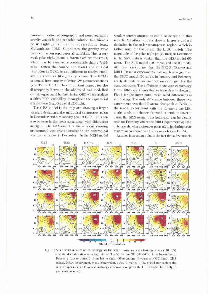
　The　observed　double　peaks　in　the　s㌃andard　deviation

around　the　stratopause　in　December，whichcon・espondtothesubtropicaljetaround300Nan〔1the

polar　night　jet　around600N　as（le丘ned　in　Kodera　an（l

Kuroda（2002），were　not　evidentin　thめGCMs．In　most

GCMs　the　standard、deviation　at　high　latitudes　was

already　strong　in　early　lwinter，e．g．，』in　the　FUB，the

MRH　and　the　UIUC　models．In　the　case　of　the　FUB

mo（1el　this　is・probably4ue　to　its　large　intemal　year－to－

year　variability　which　starts　earlier　than　observed（not

explicitly　shown　here）．None　of　the　GCMs　shows　a

polar　night　jet　similar　to　observations－this　is　a　well－

known　phenomenon，the　polar　night　jet　in　GCMs　is

con丘ned　to　high　latitudes　an（l　fails　to　tilt　equatorward．

The　strongjetleads　to　the　so－called”cold－biasll　problem

in　the　lower　stratosphere　at　high　latitudes．A

84Vol．54，No．2

parameterisation　of　orographic　and　non－orographic

gravity　waves　is　one　pmbable　solution　to　achieve　a

polar　night　jet　similar　to　observations（e．g．，

McLandress，1998）。Sometimes，the　gravity　wave

parameterisation　suppresses　all　variability．Then　a　very

weak　polar　night　jet　and　a”warm－bias”are　the　result，

which　may　be　even　more　problematic　than　a”cold－

bias”．Often　the　coarse　horizontal　and　vertical

resolution　in　GCMs　is　not　su伍cient　to　resolve　sma11－

scale　structures　like　gravity　waves．The　GCMs

presented　here　employdi丘ering　GWparameterisations

（see　Table1）。Another　important　aspect　for　the

discrepancy　between　the　observed　and　modelled

climatologies　could　be　the　missing　QBO　which　produce

a　fairly　high　variability　throughout　the　equatorial

stratosphere（e．g．，Gray　et　aL，2001a，b）．

　The　GISS　model　is　the　only　one　showing　a　larger

standard　deviation　in　the　subtropical　stratopause　region

in　December　and　a　secondaly　peak　at650N．This　can

also　be　seen　in　the　mean　zonal　mean　wind　differences

in　Fig。5。The　GISS　model　is　the　only　one　showing

pronounced　westerly　anomalies　in　the　subtropicaI

stratopause　region　in　December．In　the　MRH　mode1

weak　westerly　anomalies　can　also　be　seen　in　this

month。All　other　models　show　a　larger　standard

deviation　in　the　polar　stratopause　region，which　is

rather　small　for　the　IC　and　the　UIUC　models．The

magnitude　of　the　polamightjet（70m／s）in　December

in　the　NMC　data　is　weaker　than　the　GISS　mode1（90

m／s）．The　FUB　mode1（100m／s），and　the　IC　mode1

（80m／s）are　stronger　than　the　MRI－G（60m／s）and

MRH（60m／s）experiments，and　much　stronger　than

the　UIUC　mo（1el（50m／s）。In　January　and　February

nearly　all　model　winds　are10－30m／s　stronger　than　the

observed　winds。The（iifference　in　the　wind　climatology

forthe　MRI　experiments　thatwe　have　already　shown　in

Fig．5fo1・the　mean　zonal　mean　wind　differences　is

interesting．The　only　difference　between　these　two

experiments　was　the2－D－ozone　challge　field．While　in

the　model　experiment　with　the　IC　ozone　the　MRI

model　tends　to　enhance　the　wind，it　ten（ls　to　lower　it

using　the　GISS　ozone．This　behaviour　can　be　clearly

seen　for　Febmarywhere　the　MRI－I　experimentwas　the

only　one　showing　a　stronger　polar　nightjet　during　solar

maximum　compared　to　all　othermodels（see　Fig．5）．

　Another　interesting　pointis　the　factthat　a　fewmodels

　　　　　　　　　口　　　　　　　”　　　　　　　”　　　　　　　11　　　　　　　”　　　　　　　11　　　　　　　η　　　　　　　　　　　　　　　　　　　　　　　　　　　　　　　　　　　　　　　　　　　　　　　　　　　　　　　　　　　　IC　　　　OBS　　　　　　　　　　　　　　　GISS　　　　　　　　　　　　　　　　　　　　　　　　　MRl－G　　　　　　　　　　　　　　　　　　　　　　　　　　　　　　　　　　　　　M　Rl－i　　　　　　　　　　　　　　　　　　　　　　　　　　　　　　　　　　　　　　　　　　　　　　　　FU8　　　　　　　　　　　　　　　　　　　　　　　　　　　　　　　　　　　　　　　　　　　　　　　　　　　　　　　　　　　　　　　　　　　　　　Ul　UC

2㎝40R60R1騨20腰欄酬1騨 2㎝姻6傭1騨

　1

10

100

850　　2Q鯛　40麗　60緯　8D睡　　　　2Q斜　40葭　60睡　80鱒　　　　　　　　　1　　　　　　　　　　　　　1　　　　　　　　　　　　　　　　　　　　　　　　20國　　40髄　　60踵　　80鰻　　　　　　　　　　　　　　　　　　　　　　　　　　　　　　　1

20撞40誕60㌧騨 20劉40網60N1勢瞬20“0漣60制1蓼髄

2G紺酬60牒1酬　　　　　　　　　　　20婦40H60N80麗　　　　　　　　　　　　　　　　　　璽　　　　　　　　　　　　　　　　　　　　　　20短　　40N　　60鱈　　80閥　　　　　　　　　　　　　　　　　　　　　　　　　　　　　等

20阿40瑚δo赫1騨

　　　　　　　　　　　　　　　　　　　　　　　　2側40閥60N28側20闘4GN6斜28㎝　　20網　　40H　　6GN　　80閥　　　　　　　　　2　　　　　　　　　　　　　20N　　40N　　60N　　80紳　　　　　　　　　　　　　　　　　　　　2　　　　　　　　　　　　　　　　　　　　　　　　　　　　　　　　　　　　　　　　　　　　　　20鰻40瞳60随80幾　　　　　　　　　　　　　　　　　　　　　　　　　　　　　　　　　　　　　　　　　　　　　　　　　　　　　2　　　　　　　　　　　　　　　　　　　　　　　　　　　　　　　　　　　　　　　　　　　　　　　　　　　　　　　　　　　　　　　　　　　　　20網　　4Q鱒　　GON　　80健　　　　　　　　　　　　　　　　　　　　　　　　　　　　　　　　　　　　　　　　　　　　　　　　　　　　　　　　　　　　　　　　　　　　　　　　　　　2　　　　　　　　　　　　　　　　　　　　　　　　　　　　　　　　　　　　　　　　　　　　　　　　　　　　　　　　　20囲　　40樋　　60鯛　　80閥　　　　　　　　　　　　　　　　　　　　　　　　　　　　　　　　　　　　　　　　　　　　　　　　　　　　　　　　　　　　　　　　2

　1

10

100

850

、欄20輔　　40賛　　60閥　　80慢　　　　20麟　　40N　　60閥　　80闘　　　　20制　　40睡　　60懸　　80麓　　　　2｛》謎　　40N　　60肘　　80慢　　　　20周　　40囲　　60断　　80製　　　　20醤　　40湖　　60細　　80暦

20欝　　40網　　00結　80瞳

　　　　　　　1

　　20岡　40罵　60煙　80雑

騨1

StondGrd deviG圭iQn1　　　1

Fig．10：Mean　zonal　mean　wind　climatology　for　the　solar　maximum　cases（contour　interval10m／s）

　　　　　and　stan（lard　deviation（shading　intelva13m／s）for　the　NH（200－800N）from　November　to

　　　　　Febmary（top　to　bottom）；from　left　to　right：Observations（6years　of　NMC　data），GISS

　　　　　model，MRI－G　experiment，MRH　experiment，FUB，IC　mode1，UIUC　model（for　each　of　the

　　　　　mo（iel　experiments　a20－year　climatology　is　shown，except　for　the　UIUC　mode1，here　only15

　　　　　years　are　included）．

2003 GRIPS　Solar　Experiments　Intercompahson　Project：Initial　Results 85

showed　a　secondary　peak　in　the　stan（1ard　deviation

around　the　subtropical　stratopause　not　in　early　winter

（December）as　in　observations，but　a　little　bit　later．In

the　IC　model　this　can　be　clearly　seen　in　February　and

corresponds　well　with　the　westerly　wind　anomaly　in

this　region　as　seen　in　the　zonal　mean　wind　difOerences

in　Fig．5．In　the　UIUC　model，the　standard（leviation　is

very　small　in　the　upper　stratosphere，particularly，in　the

subtropics　throughout　the　winter．This　apparently

reflects　the　low　mo（lel　top　at　l　hPa，which　dampens

Planetary　waves　propagating　up　into　the　equatorial

stratopause　region．

4．20bservedv＆riations　in　ozone　and　temperature

　The　present　study　focused　mainly　on　the　differences

among　the　model　simulations。One　of　the　peculiarities

of　the　solar　influence　is　that　there　is　no　firm

observational　evidence．Observational　results　have

their　own　problems　due　to　the　shortness　of　the

homogeneous　data　sets　or　due　to　instrumental

calibrations．It　is　also　dif五cuIt　to　distinguish　the　solar

signalfrom　other　sources　ofvariability．

　There　are　difβerent　types　of　instruments　measuring

ozone　as　well　as　temperature：1）groun（i－based

instmments（radioson（1e，rocket　sonde，an（11idar），and

2）satellite　instruments（microwave，UV　and　infrared

sounders）．The　post←processing　of　satellite　data　has　to

take　into　account　problems　due　to　temporal

discontinuity・，instrument　calibration（area　and　weight

factor），an（l　orbit　drift．Especially，overlapping　pe1●iods

of　d迅erent　satellite　instmments　can　cause　pmblems　if

the　respective　time　series　have　to　be　fitted　together

（e．g．，Frohlich，2000）．There　are　further　natural

disturbances，such　as　volcanic　eruptions，which　can

lead　to　an　increase　in　the　stratospheric　aerosol　amount

for1－2years　following　the・eruption　and　influence　the

chemical　and　radiation　budget　of　the　atmosphere．

Volcanic　aerosol　also　directly　disturbs　the　satellite

measurements．Often　years　following　large　volcanic

eruptions（Mount　Agung，1963；EI　Chichon，1982；

Momt　Pinatubo，1991）are　neglected　in　data　sets　to

eliminate　these　effects．Volcanic　aerosols（sulfate

aerosols）provide　a　catalyst　for　stratospheric　ozone

depletion　an（l　counteracted　the　ozone　increase（iuring

solar　ma｝dmum　years　in　which　avolcanic　emption　took

place，i．eしin1982and1991．

　The　same　problem　of（1ata　reliability　exists　for

temperature　measurements．Satellite　basedmeasurements　are　only・available　since1979and　usually

have　quite　a　coarse　vertical　resolution．There　is　no　dat3

set　covering　the　whole　atmosphere　from　the

troposphere　up　to　the　mesosphere．Observed

temperature　signals　have　to　be　viewed　with　caution

because　they　depend　on　the　source　of　the　data

（instrument　specialities　such　as　the　vertical　resolution

etc・），th♀time　interval　of　measurements，and　the

method　with　which　the　temperature　signal　was

extracted　from　the　raw　data（Ramaswamy　et　al．，2001）．

Often　a　statistical　multiple　linear　regression　model　is

used　to　extractthe　solar　signa1．These　statistical　models

usually　take　into　account　a　linear　trend　term，a　QBO

term，an　ENSO　term，a　solar　forcing　term，and　an

aerosol　term（for　the　volcanic　signal）and　are　able　to

extractwith　this　method　each　ofthe　assumed　natural　or

anthropogenic　contributions．If　a　volcanic　signal

（warming　of　the　lower　stratosphere）coincides　with　a

wamingduetothem漉mumphaseofthesolarcycleas　happened　in1982and1991，it　is　important　to

separate　the　volcanic　and　the　solar　signal　in

temperaturetime　series（e．g．，McCormacketal．，1997）．

　The　solar　signal　in　temperature　extracted　from

different　data　sets　shows　discrepancies．For　example，

McCormack　and　Hood（1996），analysed　NMC　data

from1980to　the　year1995，and　found　positive　amual

mean　temperature　signals　due　to　the11－year　solar　cycle

of2－2．5K（from300S　to300N　near　the　stratopause

（their　Fig．4））l　of1。5K（from400－60Q　north　and　south

aromd37km　height），an（1even　negative　temperature

anomalies　in　the　equatorial　mi（ldle　stratosphere　around

32km　height．In　contrast，the　strongest　temperature

signal　in　the　WMO　report（1999），estimated　with　a

regression　model　from　SSU　and　MSU　data，suggested

O．75K　in　the　e（luatorial　upPer　stratosphere　at　a1●ound40

㎞heightwhichdecaye曲丘herupandevenreachednegative　anomalies　above50㎞．

　All　GCM　experiments　presented　here　produced　a

large　temperature　signal　of　O．75－1K　around　the

stratopause（see　Fig．4）．None　ofthe　GCMs　showed　a

negative　temperature　signal　in　the　middle　stratosphere

as　fomd　in　McCormack　and　Hood（1996）．A　similar

positive　temperature　signal　was　also　found　in　the　UIUC

GCM．The　annual　mean　temperature　differences

between15solar　maximum　and15solar　minimumyears　for　this　model　are　shown　in　Fig．11．They　can　be

directly　compared　with　Fig．4．Although　the　top　of　this

GCM　is　close　to　the　stratopause，it　showed　a　quite

similar　temperature　response　to　the　other　GCMs，

featuringhighertemperatures　ofO．75－1Karomd　l　hPa．

These　results　suggest　that　the　interactively　calculated

ozone（loes　not　give　a　qualitatively　different　or　better

response　than　the　GCM　experiments　using　specified

ozone．The　impact　of　interactively　calculated　ozone

should　be　further　studied　with　other　GCMs　extending

into　themesosphere．

86

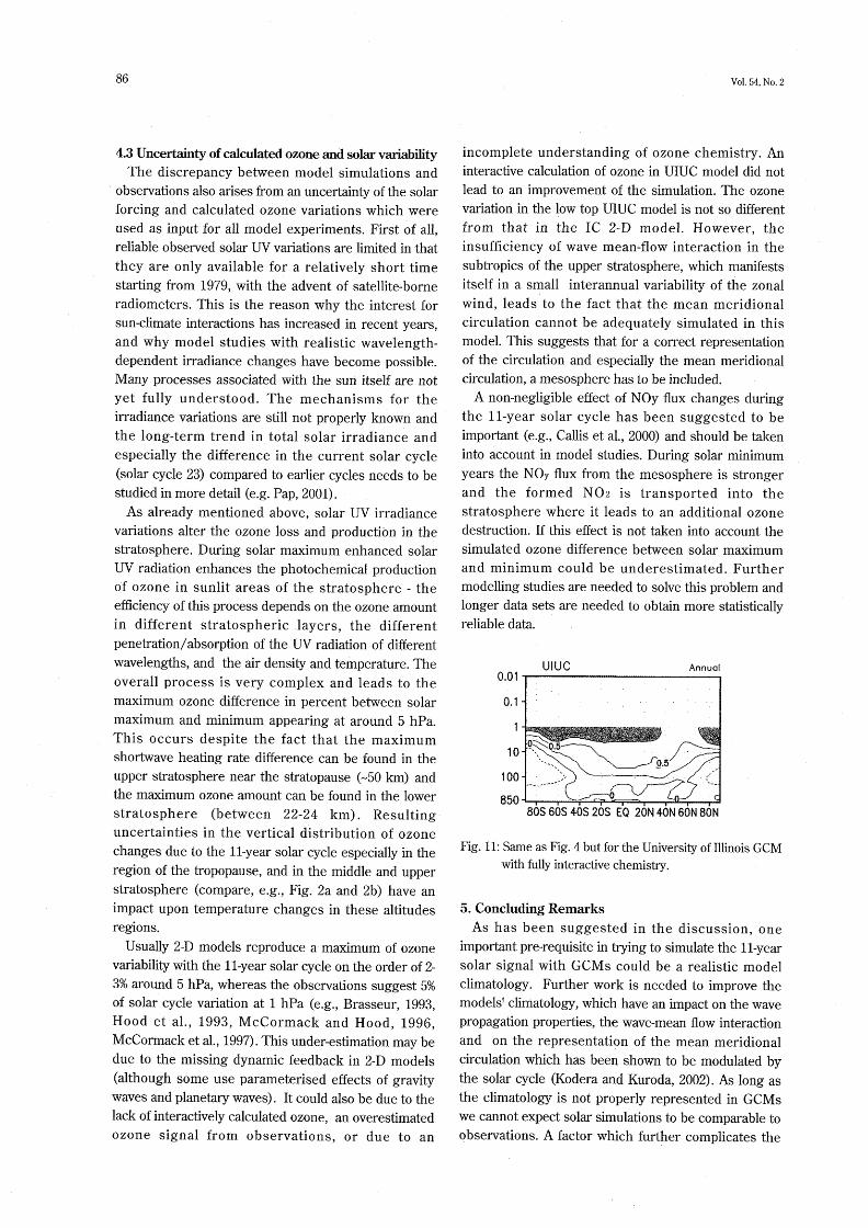
4．3Uncertαinty　ofcalculated　ozone　and　solarvahab皿ty

　　The　discrepancy　between　model　simulations　and

observations　also　arisesfrom　an　mcertainty　ofthe　solar

forcing　an（l　calculated　ozone　variations　which　were

used　as　input　for　all　model　experiments．First　of　all，

reliable　observed　solar　UVvariations　are　limited　in　that

they　are　only　available　for　a　relatively　short　time

starting　from1979，with　the　a（1vent　of　satellite－bome

radiometers．This　is　the　reason　why　the　interest　for

sun－climate　interactions　has　increased　in　recent　years，

and　why　mo（iel　studies　with　realistic　wavelength－

dependent　irradiance　changes　have　become　possible．

ManyF　processes　associated　with　the　sun　itself　are　not

yet　fully　understood．The　mechanisms　for　theirradiance　variations　are　still　not　properly　known　and

the　long－term　trend　in　total　solar　irradiance　and

especially　the（lifference　in　the　current　solar　cycle

（solar　cycle23）compared　to　earlier　cycles　needs　to　be

studied　in　more　detai1（e．g．Pap，2001）．

　　As　already　mentioned　above，solar　UV　irradiance

variations　alter　the　ozone　Ioss　and　productiOn　in　the

stratosphere．During　solar　maximum　enhanced　solar

UV　radiation　enhances　the　photochemical　production

Of　ozone　in　sunlit　areas　of　the　stratosphere－the

ef且ciency　ofthis　process　depends　on　the　ozone　amount

in　different　st1●atospheric　layers，the　different

penetration／absorption　of　the　UV’ra（liation　of（1迂ferent

wavelengths，and　the　air　density　and　temperature．The

overall　process　is　very　complex　and　leads　to　the

maximum　ozone　difference　in　percent　between　solar

maximum　and　minimum　apPearing　at　around5hPa．

This　occurs　despite　the　fact　that　the　maximum

shor伽ave　heating　rate　difference　can　be　foun（i　in　the

upper　stratosphere　near　the　stratopause（～50km）and

the　maximum　ozone　amount　can　be　found　in　the　Iower

stratosphere　（between　22－24　km）．Resulting

uncertainties　in　the　vertical　distribution　of　ozone

changes（lue　to　the11－year　solar　cycle　especially　in　the

region　of　the　tropopause，and　in　the　middle　and　upper

stratosphere（compare，e．g．，Fig．2a　and2b）have　an

impact　upon　temperature　changes　in　these　altitudes

regions．

　　Usually2－D　models　reproduce　a　ma》dmum　of　ozone

variabilitywith　the11－year　solar　cycle　on　the　order　of2－

3％aroun（15hPa，whereas　the　obse坪ations　suggest5％

of　solar　cycle　variation　at　l　hPa（e．g．，Brasseur，1993，

Hood　et　aL，1993，McCormack　and　Hood，1996，

McCormacketal．，1997），Thisunde卜estimationmaybe

due　to　the　missing　dynamic　feedback　in2－D　models

（although　some　use　parameterised　effects　of　gravity

waves　and　planetarywaves）．It　could　also　be　due　to　the

lack　ofinteractively　calculated　ozone，an　overestimated

ozone　signal　from　observations，or　due　to　an

Vol，54，No．2

incomplete　understanding　of　ozone　chemistry．An

interactive　calculation　of　ozone　in　UIUC　model　did　not

lead　to　an　improvement　of　the　simulation．The　ozone

variation　in　the　low　top　UIUC　model　is　not　so　d迂ferent

from　that　in　the　IC2－D　modeL　However，the

insufficiency　of　wave　mean－flow　interaction　in　the

subtropics　of　the　upper　stratosphere，which　manifests

itself　in　a　small　interannual　variability　of　the　zonaI

wind，1eads　to　the　fact　that　the　mean　meridionaI

circulation　cannot　be　ade（luately　simulated　in　this

modeL　This　suggests　that　for　a　correct　representation

of　the　circulation　and　especia11y　the　mean　meridional

circulation，a　mesosphere　has　to　be呈ncluded．

　Anon－negligibleeffectofNOyfluxchangesduringthe11－year　solar　cycle　has　been　suggested　to　be

important（e．g．，Callis　et　al．，2000）and　shoul（i　be　taken

into　account　in　model　studies．During　solar　minimum

years　the　NOy　flux　from　the　mesosphere　is　stronger

an（1the　formed　NO2is　transported　into　the

stratosphere　where　it　leads　to　an　additional　ozone

destruction．If　this　eぜect　is　not　taken　into　account　the

simulated　ozone　difference　between　solar　maximum

and　minimum　could　be　underestimated．Furthermodelling　studies　are　needed　to　solve　this　problem　and

longer　data　set5are　nee（led　to　obtain　more　statistically

reliable　da惚．

0，01UlUC AnnUG！

0．1

110

100

850

9。5

80S60S40S20S　E：Q20N40N60N80N

Fig．11：Same　as　Fig．4butforthe　University　ofIllinois　GCM

　　　　　with　fullyinteractive　chemistry．

5。Concluding　Remarks

　As　has　been　suggested　in　the　discussion，one

importantpre．requisite　in　trying　to　simulate　the11－year

solar　signal　with　GCMs　could　be　a　realistic　model

climatology．Further　work　is　needed　to　improve　the

modelsl　climatology，which　have　an　impact　on　the　wave

propagation　properties，the　wave－mean　flow　interaction

and　on　the　representation　of　the　mean　meridional

circulation　which　has　been　shown　to　be　modulated　by

the　solar　cycle（Kodera　and　Kuroda，2002）．As　long　as

the　climatology　is　not　properly　represented　in　GCMs

we　camot　expect　solar　simulations　to　be　comparable　to

observations。A　factor　which　further　complicates　the

2003 GRIPSSolar　ExperimentsIntercomparison　Project二InitialResults 87

solar　signal　is　the　QBO．

　　The　GISS　model　appeared　to　show　a　zonal　mean

response　most　like　the　obselvations　in　the　NH　even

though　its　wind　climatology　was　not　better　than　the

other　GCMs（except　for　December　where　it　was　the

only　GCM　showing　a　higher　standard　deviation　in　the

subtropical　stratopause　region）．This　could　be　one

reason　for　its　relatively　good．correspondence　with

obselvations．It　was　however　dif且cult　to　select　a”best”

model　for　representing　both　hemispheres　adequately．

Ittumed　outthatthe　GCMswere　sensitiveto　the　ozone

change　fie1（1which　can　be　clearly　seen，not　only　by

comparingthe　different　GCMs　thatused　the　two　ozone

change　fields，but　also　by　comparing　the　simulations

usingthetwo　ozone　change且eldsinthesame　GCM。

　　From　all　points　discussed　one　could　speculate　that

the”unrealistic”（lynamics　in　the　models　lead　to　a

temperature　signal　that　is　mainly　radiatively　controlled

in　early　winter．In　later　winter　the　signal　is　a

combination　of　radiative　effects　in　the　models

（dependent　on　the　radiation　schemes）an（l　intemal

mode1（iynamics，which　is　not　comparable　to

observations．Improving　the　model　climatologies　and

』therefore　the　dynamics　could　maybe　Iead　to　a

temperature　signal　that　is　more　comparable　with

observations．In　summary，to　achieve　a　better

understan（iing　and　for　better　（lefining　future

comparison　studies，the　model　climatologies　nee（l　to　be

improved　and　the　ozone　difference　between　solar

maximum　and　minimum　need　to　be　further　studied

with　chemistry　models．Also，the（lerivations　of

observed　solar　signals　in　temperature　and　ozone　need

to　be　improved．

6．Acknowle（1gementsWe　would　like　to　thank　J．Lean　for　providing　the

wavelength－depen（1ent　solar　irradiance　data　and　S．

Pawson　for　the　coordination　ofthe　GRIPS　project．This

work　is　supported　in　part　by　a　Bilateral　Intema．tional

Joint　Research　Program　of　the　Japanese　Agency　for

Science　andTechnology，an（1resulted　from　two　stays　of

the　first　author（K爾a　Matthes）at　the　Meteorological

Research　Institute（MRD　inTsukuba，Japan．The　study

has　also　been　partly　fun（ied　by　the　European

Commission　under　the　contract　No．EVK2－CT－1999－

00001（SOLICE）．The　integrations　with　the　FUB－

CMAM　and　further　diagnostics　were　perfomled　on　the

CRAY　J932／16－81920f　the　Konrad－Zuse－Zentrum　fur

I㎡omationstechnikBerlin（ZIB）．

7．ReferencesBrasseur，G．，1993：The　response　of　the　mi〔1dle　atmos－

　　　phere　to　long－term　and　short－term　solar　variability：

　　　A　two－dimensional　modeL∫。060ρ勿s．1～6s．，98，

　　　23079－23090．

Briegleb，B．P．，1992：Delta－Eddington　approximation

　　　for　solar　radiation　in　the　NCAR　community　climate

　　　model．1．θ60ゆhダs．1～6s．，97，7603－7612．

Ca11is，L．B．，M．Natarajan，and　J．D．Lambeth，2000：

　　　Calculated　upPer　stratospheric　effects　of　solar　UV

　　　nux　an（l　NOy　variations（玉uring　the11－year　solar

　　　cycle．（｝60プ》hタs．ム～θ3．Lα孟．，27，3869－3872．

Chou，M．D．，1990：Parameterizations　for　the　absorp－

　　　tion　of　solar　radiation　by　O2and　CO2with　applica－

　　　tion　to　climate　studies，∫．α伽．，3，209－217．

Chou，M．D．，1992：A　solar　radiation　model　for　use　in

　　　climate　studies，1．14枷os．S6歪．，49，762－772．

Chou，M．D．，and　K。T．L£e，1996：Parameterization　for

　　　the　absorption　ofsolar　radiation　bywatervapor　and

　　　ozone，∫．ノ1渉盟zos．Soづ．，53，1203－1208．

Chou，M．D．，and　M．」．Suarez，1999：A　solar　radiation

　　　parameterization　for　atmospheric　studies，in

　　　Technical　Report　Series　on　Global　Modeling　and

　　　Data　Assimilation，v．15，40pp．，NASA　Greenbelt，

　　　Md．

Edwards，J．M．，andA．Slingo，1996：Studieswith　afle》d－

　　　ble　new　radiation　code．1：Choosing　a　configuration

　　　for　a　large－scale　mode1，Q．∫．1～．〃i6孟60zoJ．Soo．，122，

　　　689－719．

Fortuin，J．P．F．，αnd　U．Langematz，1994：An　update　on

　　　the　global　ozone　climatology　and　on　concurrent

　　　ozone　and　temperature　trends，SPIE　Atmospheric

　　　SensingandModeling，2311。

Fouquart，Y．，and　B．Bonne1，1980＝Computations　of

　　　solar　heating　of　the　Earthls　atmosphere：a　new

　　　parameterization，Beitr．Phys．Atmos．，52，1－16．

Fr6hlich，C．，2000：0bservations　of　Irra（liance

　　　Measurements。S釦66S厩．1～ω．，94，15－24．

Gray，L．」．，E．F．Drysdale，T．J．Dunkerton，and　B．N．

　　　Lawrence，2001a：Model　studies　ofthe　interamuaI

　　　variability　of　the　Northem　Hemisphere　stratos－

　　　pheric　winter　circulation：the　role　of　the　Quasi

　　　Biennia10scillation．Q．∫．ノ～．ハ4θ≠6070」．Soo．，127，

　　　1413－1432．

Gray，L．J．，S，J．PhipPs，T．J．Dunkerton，M．P．Baldwin，

　　　E．F．Drysdale，and　M．R．Allen，2001b：A　data

　　　study　of　the　influence　of　the　e（luatorial　upper

　　　stratosphere　on　Northem　Hemisphere　stratospher－

　　　ic　sudden　warmings．Q．1．R．ハ4伽070」．Soc．，127，

　　　1985－2003．

Haigh，J．D．，1994：The　role　of　stratospheric　ozone　in

　　　modulating　the　solar　radiative　forcing　of　climate．

　　　梅オz6zo，370，544－546．

Haigh，」．D．，1996：The　impact　of　solarvariability　on　cli－

　　　mate．So伽oε，272，981－984．

Haigh，J．D．，1999：A　GCM　study　of　climate　change　in

88

　　　response　to　the11－Year　solar　cycle．Q．∫．1～．

　　　M6陀ozoJ．So6．，125，871－892．

Hansen，」．，G．Russell，D．Rin（1，P．Stone，A．Lacis，S．

　　　Lebedeff，R．Ruedy，an（l　L．Travis，1983：Efficient

　　　three－dimensional　global　models　for　climate　stud－

　　　ies：Models　I　and　II．Mo％．晩α云h671～θ∂．，111，609－

　　　662．

Keating，G．M．，D．F．Young，and　M．C．Pitts，1987：0zone

　　　reference　models　for　CIRA，∠4吻．助α681～6s．，7，105－

　　　115．

Kodera，K．，1991：The　solar　and　eq．uatorial　QBO

　　　Influences　on　the　stratospheric　circulation　during

　　　early　northem　winter．060望）hタs．1～εs．五観．，18，1023－

　　　1026．

Kodera，K．，1995：0n　the　origin　and　nature　of　the　inter－

　　　annual　variability　of　the　winter　stratospheric　circu－

　　　lation　in　the　northem　hemisphere．1．060ρhッs．1～6s．，

　　　100，14077－14087．

Kodera，K．，and　Y．Kuroda，2002：Dynamical　response

　　　tothesolarcycle．∫．0θoρhツs．1～6s．，107，4749，

　　　（10i：10．1029／2002JDoo2224．

Kodera，K．，K。Matthes，K．Shibata，U。Langematz，and

　　　Y．Kuroda，2003：Solar　impact　on　the　lower　mesos－

　　　pheric　subtropical　jet：a　comparative　study　with

　　　general　circulation　model　simulations，060ρhッs．

　　　1～θs．L観．，30（4），1175，doi：10．1029／2002GLO16584．

Kuroda，Y．，an（1K．Kodera，2001：Variability　of　the

　　　polar－night　jet　in　the　northem　and　southem　hemi－

　　　spheres．∫．（ヌ60ρh‘ys．1～6s．，106，20703－20713．

Kuroda，Y．，an（i　K．Kodera，2002：Effect　of　the　sola．r

　　　cycle　on　the　Polar－Night　Jet　Oscillation．1．ハ4α．Soo．

　　　ノ41）α％，80，973－984．

Labitzke，K．，1987：．Sunspots，the　QBO　and　the　stratos－

　　　phericItemperature　in　the　north　polar　region．

　　　060φhタs、五～6s．Z，α渉。，14，535－537．

Labitzke，K．，2001：The　global　signal　of　the11－Year

　　　sunspot　cycle　in　the　stratosphere：Differences

　　　between　solar　ma｝dma　and　minima．〃1εオ．Z醜s6h峨，

　　　10，901－908．

Labitzke，K．，and　H．v。Loon，1988：Associations

　　　between　the11－year　solar　cycle，the　QBO　and　the

　　　atmosphere，Part　I：The　troposphere　and　stratos－

　　　phere　in　the　Northem　Hemisphere　in　Winter．∫．

　　　ノ1オ〃¢os．7167名月21ソs．，50，197－206．

Labitzke，K．and　H．v．Loon，1999：The　stratosphere：

　　　phenomena，history，an（l　relevance．Springer

　　　Verlag，Berlin．

Langematz，U．，2000：An　estimate　ofthe　imp＆ct　of

　　　observed　ozone　Iosses　on　stratospheric　tempera－

　　　tures．060φhタs．1～os．Lα！．，27，2077－2080。

Langematz，U．，and　S．Pawson，11997：The　Berlin　tropos－

　　　phere－stratosphere－mesosphere　GCM：climatology

　　　and　annual　cycle．（ン．∫．1～．ノ砿6オ60名oJ．So6．，123，1075一

VoL54，No．2

　　　1096．

Larkin，A．，J．D．Haigh，and　S．Djavidnia，2000：The

　　　Effect　of　solar　UV　radiation　variations　on　the

　　　Earth夕s　atmosphere．助α66S6∫．1勧．，94，199－214．

Lean，J．L．，G．J。Rottman，H．L　Kyle，T．N．Woods，J．R

　　　Hickey，and　L．C．Puga，1997：detection　an（l　para－

　　　meterisation　of　variations　in　solar　mid－and　near－

　　　ultraviolet　radiation（200－400nm）．∫．（｝60φh夕s．1～6s．，

　　　102，29939－29956．

McCormack，J．P．，and　L．L．Hood，1996：ApParentsolar

　　　cycle　variations　of　upPe1●stratospheric　ozone　and

　　　temperature：latitude　and　seasonal　dependences．1．

　　　（3！60メ）hダs．R6s．，101，20933－20944．

McComack，J．P．，L．L．Hood，R．Nagatani，A．」．Miller，

　　　W．G．Planet，and　R．D．McPeters，1997：　　　Appro》dmate　separation　ofvolcanic　an（111－year　sig－

　　　nals　in　the　SBU▽一SBUV／2toねl　ozone　record　over

　　　the1979－1995period，（3！80ρhダs．Rεs．Z，8か．，24，2729－

　　　2732．

McLandress，C．，1998：0n　the　importance　of　gravity

　　　waves　in　the　middle　atmosphere　and　their　parame－

　　　terization　in　general　circulation　models．1．z4加os．

　　　SoJ．一丁蹴P勿s．，60，1357－1383．

Pap，J．M．，2001：Totalsolarand　spectralirradiancevari－

　　　ations　from　near－UV　to　infrared，in：The　variable

　　　shape　of　the　Sun：Astrophysical　Consequences．ed．

　　　」．P．Rozelot，Lecture　Notes　in　Physics，Springer－

　　　Verlag，in　press．

Pawson，S．，U．Langematz，G．Radek，U．Schlese，and　P．

　　　Strauch，1998：The　Berlin　troposphere－stratos一

　　　『phere．mesosphere　GCM：sensitivity　to　physical

　　　parameterizations．g．∫。R．ハ4吻070」．So6。，124，

　　　1343－1371．

Pawson，S．，K．Ko（lera，K．Hamilton，T．G．Shepherd，S．

　　　R．Beagley，B．A．Bov皿e，J．D．Farrara，T．D．A．

　　　Fairlie，A．Kitoh，W．A．Lahoz，U．Langematz，E．

　　　Manzini，D．H．Rind，A．A．Scaife，K．Shibata，P．

　　　Simon，R　Swinbank，L　Takacs，R　J．Wilson，J．A．

　　　A1－Saadi，M．Amode，M．Chiba，L．Coy，J．de

　　　Grandpre，RS．Ec㎞an，M．Fiorino，W．L．Grose，

Ramaswamy，V

H．Koide，J．N．Koshyk，D．Li，J．Lerner，J．D．

Mahlman，N，A．McFarlane，C．R．Mechoso，A．

Molod，A．OINeill，R．B．Pierce，W．」．Randel，R．B．

Rood，F．Wu，2000：TheGCM－Re譜tyIntercomparison

Project　for　SPARC（GRIPS）：Scientific　Issues　and

Initial　Results．B％JJ．ノ1％z．M6！εo名oJ．So6．，81，781－796。

　　　　　　　　．，M．L．Chanin，J．Angell，J．Bamett，D．

Gaffen，M．Gelman，P．Keckhut，Y．Koshelkov，K．

Labitzke，J．」．R．Lin，A．0’Neil，J．Nash，W．Rande1，

R．Rood，M．Shiotani，R．Swinbank，and　K．Shine，

2001：Stratospheri¢temperature　trends：observa－

tions『and　model　simulations．Rω．（｝θoρhダs．，39，71－

122．

2003 GRIPS　SolarExperiments　Intercomparison　Project：Ini滅al　Results 89

Randel，W．」．，1992：Global　atmospheric　circulation　sta．

　　　tistics，1000－1mb，NCAR　Tech．Note．NCAR／TN．

　　　366＋STR，256pp．，Nat．Cent．for　Atmos．Res．，

　　　Boulder，Colora（lo．

Rin（1，D。，R　Suozzo，N．K．Balachandran，A．Lacis，and

　　　G．Russe1，1988a：The　GISS　global　climate－middle

　　　atmosphere　model，Part　ll　Model　structure　and　cli－

　　　matology．1．z4伽os．S6ぎ．，45，329－370．

Rind，D。，R．Suozzo，and　N．K．Balachandran，1988b：

　　　The　GISS　Global　Climate－Middle　atmosphere

　　　mode1．Part2：Modelvariability　due　to　interactions

　　　between　planetary　waves，the　mean　circulations，

　　　and　gravitywave　drag．∫．ノ4醜os．So∫．，45，371－386．

Rozanov，E．V．，Schlesinger，M．E．，and　Zubov，V．A．，

　　　2001：The　University　of皿inois，Urbana－Champaign

　　　three－dimensional　stratosphere－troposphere　gener－

　　　al　circulation　model　with　interactive　ozone　photo－

　　　chemistry：F置een－year　control　run　climatology．∫．

　　　0卿勿s．1～6s．，106，27233－27254．

Salby，M．，and　P．Callaghan，2000：Comection　between

　　　the　solar　cycle　and　the　QBO：The　Missing　link．∫．

　　　α魏．，13，2652－2662。

Shibata，K．，and　A．Uchiyama，1994：An　application　of

　　　the　discrete　ordinate　method　to　terrestrial　radiation

　　　in　climate　models．∫．z4枷os．S6ゼ．，51，3531－3538．

Shibata，K．，H．Yoshimura，M．Ohizumi，M．Hosaka，

　　　and　M．Sugi，1999：A　simulation　oftroposphere，

　　　stratosphere　andmesospherewithanMRI／JMA98　　　GCM。P砂θ鴬初1晩！εo名oJ。α％4060ρ勿s．，50，15－53．

Shinde11，D．，D．Rind，N．Balachandran，」．Lean，and　J．

　　　Lonergan，1999：Solar　cycle　variability，ozone，and

　　　climate．So歪8銘66，284，305－308．

Shinde11，D．T．，G．A．Schmidt，R．L．Miller，and　D．Rind，

　　　2001：Northem　hemisphere　winter　climate

　　　response　to　greenhouse　gas，ozone，solar，and　vol－

　　　canic　forcing．1．（360ρhダs．1～8s。，106，7193－7210．

Shine，K．P．，and　J．A．Rickaby，1989：Solar　radiative

　　　heating（lue　to　the　absorption　by　ozone，Ozone　in

　　　the　Atmosphere，R．D．Bojkov　and　P．Fabian，Eds．，

　　　Deepak，597－600．

Soukharev，B．E．，and　L．Hood，2001：Possible　sola1’

　　　mo（1ula．tion　of　the　equatorial　Quasi－Biennia1

　　　0scillation：Additional　statistical　evidence．∫，

　　　060望りhys．ム～6s．，106，14855－14868．

Strobe1，D．F．，1978：Parameterisation　ofthe　atmospher－

　　　icheatingrate丘om15to120㎞duetoO2andO3　　　absorPtion　of　solar　radiation，1．060φhタs．1～6s．，83，

　　　6225－6230．

Swinbank，R．，W．A．Lahoz，A　ONeill，C．S．Douglas，A．

　　　Heaps，and　D．Podd，1998：Middle　atmospherevari－

　　　ability　in　the　UK　Meteorological　Office　Unified

　　　Model．Q．1．1～．M伽o名oJ．Soo．，124，1485－1525．

van　Loon，H．，and　K．Labitzke，2000：The　innuence　of

　　　the11－year　solar　cycle　on　the　stratosphere　below

　　　30km：Areview．助αoθS6盛1～θ∂s．，94，259－278．

Wang，W．一C．，X．一Z．Liang，M．P．Dudek，D．Pollard，and

　　　S。L　Thompson，1995：Atmospheric　ozone　as　a　cli－

　　　mate　gas．z4吻osρh副oRεs6ακh，37，247－256．

World　Meteorological　Organization，1999：Scientific

　　　assessment　of　ozone　depletion1998．Globa10zone

　　　Res．andMonit．Proj．，Rep．44，Geneva．

90 Vol．54，No．2

GRIPS太陽影響モデル実験比較計画：第1報

K．Matthes，K．Kodera，J．D．Haigh，D．T．Shlnde”，K。Shibata，

　　　　U．Langematz，E　Rozanov，and　Y．Kuroda

　GRIPS（中層大気大循環モデル国際比較計画）のうち11年太陽周期の大気に及ぼす影響に的を絞ったGRIPS参加各グル

ープの大循環モデルによる数値実験の結果を示す。ここでは、将来のより詳細な太陽活動の影響の数値実験を行う上で、

何が問題であるか明らかにすることを目的として比較を行う。それぞれの大循環モデル実験の結果がこれまでの実験や

観測に比較して整合性のあるものかの吟味を行っている。より整合の取れた比較を行うために各大循環モデルには同一

の、i）波長依存性をもつ太陽放射変化とii）それによって生じるオゾン変化を2次元光化学モデルで計算したものの双方を

与えた。各モデル実験の比較の結果には明らかな違いが見られ、これはモデル間、あるいは観測との気候値の違いを反

映していることが示唆される。この実験比較における大きな困難の一つは、モデル実験と比較する信頼できる気温やオ

ゾンの太陽周期変化の影響の観測データが無い事による。また、モデルを駆動するのに与えた太陽エネルギー・スペク

トラムやオゾンにもいまだ不確実性が残っている。