Goethe-Universität FrankfurtGoethe Center for

Scientific Computing

G-CSCReport

2011

Goethe-Zentrum für Wissenschaftliches RechnenGoethe-Universität Frankfurt

Prof. Dr. Gabriel WittumURL: http://www.gcsc.uni-frankfurt.de/

E-mail: wittum@g-csc.dePhone: +49-69-798 25258Fax: +49-69-798 25268

Table of Contents

Table of Contents ………………………………………………………………………………………3

Overview ………………………………………………………………………………………………5Introduction ………………………………………………………………………………………5The Department Simulation and Modelling (SiM), Project Overview ………………………………………5

Theses ……………………………………………………………………………………10Awards ……………………………………………………………………………………11Academic Offers to G-CSC(SiM)/SiT Members …………………………………………………11Selected Cooperations ………………………………………………………………………11Conferences, Workshops and Seminars ………………………………………………………12G-CSC (SiM) Members ………………………………………………………………………13

The Interdisciplinary Research Group Computational Finance (CoFi) ……………………………………13

Selected Project Reports …………………………………………………………………………………14A1: Modelling Barrier Membranes …………………………………………………………………………14A2: Neuroscience and Computational Medicine:

A2.1: NeuRA: The Neuron Reconstruction Algorithm …………………………………………………18A2.2: Modelling the Nuclear Calcium Code ……………………………………………………………20A2.3: Electric Signalling in Neurons …………………………………………………………………22A2.4: Modelling Replication Dynamics of Hepatitis C Virus in 3D Space …………………………………24A2.5: NeuClass: Neuron Classification Tools …………………………………………………………26A2.6: Modelling the Hydrodynamics of Synaptic Vesicles ………………………………………………27

A3: Computational Finance A3.1, CF3: The Numerical Pricing of Options with Many Risk Factors ……………………………………29A3.2, CF4: Credit Risk Estimation in High Dimensions …………………………………………………31A3.3, CF5: Portfolio Optimisation ……………………………………………………………………33

A4: Process Engineering:A4.1: Simulation of Crystal Growth and Attrition in a Stirred Tank ………………………………………35

A5: Environmental Science and Energy Technology:A5.1: Density-Driven Flow in Porous Media ……………………………………………………………37A5.2: The Software Tool r3t and Flux-Based Level-Set Methods …………………………………………39A5.3: Fractured Porous Media ………………………………………………………………………41A5.4: Modelling Biogas Production …………………………………………………………………43

A6: Computational Fluid Dynamics:A6.1: Turbulence Simulations and Application to a Static Mixer …………………………………………45A6.2: Discontinuous Galerkin Method for Incompressible Navier-Stokes Equations…………………………47A6.3: Multiphase Flows ……………………………………………………………………………49

A7: Computational Electromagnetism: A7.1: The Low Frequency Case ………………………………………………………………………51A8: Reduction of Numerical Sensitivities in Crash Simulations ………………………………………………53A10, M9, T8: 3D Visualisation of Heidelberg Castle in 1680 …………………………………………………55A11: Computational Acoustics: Eigenmodes of Musical Instruments …………………………………………57M1: Fast solvers for Large Systems of Equations: FAMG and Transforming Iterations ……………………………59

Table of Contents 3

M2: Modelling and Multiscale Numerics M2.1 Multiscale Modelling of Biological Tissue ……………………………………………………………63M2.2 Multiscale Numerics, Homogenisation and Coarse Graining ……………………………………………65M3: Finite Volume Element Methods of Arbitrary Order ……………………………………………………67M4: Level Set Methods …………………………………………………………………………………69M5: Parameter Estimation:M5.1: Parameter Estimation for Bingham Fluids and Optimal Geometrical Design of Measurement Devices ………71M5.2: Parameter Estimation for Calcium Signalling …………………………………………………………73M8, M9, T7: Geometry Modelling and Grid Generation ……………………………………………………75

Software Tools:T4: Visualisation: VRL/UG Interface ………………………………………………………………………81T5: Simulation Software Library SG ………………………………………………………………………83T8: NeuGen …………………………………………………………………………………………85T9: NeuTria …………………………………………………………………………………………86

RG: Computational FinanceCF1: Asset Management in Insurance………………………………………………………………………87CF2: Valuation of Performance Dependent Options …………………………………………………………88

List of Selected Publications 2006 - 2012……………………………………………………………………90

4 Overview

OverviewIntroductionThe present report gives a short summary of the research of the Goethe Center for Scientific Computing (G-CSC) ofthe Goethe University Frankfurt. G-CSC aims at developing and applying methods and tools for modelling andnumerical simulation of problems from empirical science and technology. In particular, fast solvers for partialdifferential equations (i.e. pde) such as robust, parallel, and adaptive multigrid methods and numerical methods forstochastic differential equations are developed. These methods are highly adanvced and allow to solve complex prob-lems..

The G-CSC is organised in departments and interdisciplinary research groups. Departments are localised directly at theG-CSC, while the task of interdisciplinary research groups is to bridge disciplines and to bring scientists form differentdepartments together. Currently, G-CSC consists of the department Simulation and Modelling and theinterdisciplinary research group Computational Finance.

The Department Simulation and Modelling (SiM)In January 2009, 22 researchers moved from Heidelberg to Frankfurt to start this new center. In Heidelberg, the groupformed the department “Simulation in Technology” and did research and development of methods for solving typicalproblems from computational biology, fluid dynamics, structural mechanics and groundwater hydrology. The mainfocus was on the development of the simulation environment ⋲, which is the first parallel and adaptive multigrid sol-ver for general models based on partial differential equations (pde).

In Frankfurt, the group now forms the department Simulation and Modeling of the G-CSC. Besides continuing the workfrom Heidelberg, we have now added new topics from finance, neuroscience and sustainable energy. Currently, G-CSCis running a total of thirty projects dealing with the simulation of a very wide variety of application problems, simulationmethods and tools.

From 2005-2010, the research focused on applications from the following areas:

A1 Computational Pharmaceutical Science: Diffusion of xenobiotics through human skin.As early as 1993, we researched diffusion through human skin and predicted diffusion pathways from our simu-lations. To match experimentally measured data, we had to postulate new diffusion pathways which were not inaccordance with traditional assumptions. When we presented the model in 1993 on the annual conference ofthe “Controlled Release Society” in Washington D.C., the paper was awarded a prize as the best paper of theconference. The results were published; however, pharmacists still kept to their old assumptions on diffusionpathways. In 2003, however, a group from MIT was able to confirm our results experimentally. This shows thatsimulation is playing an increasingly important role in biosciences as well. Meanwhile we are working on moredetailed models. More details can be found in Project A1.

A2 Computational Neuroscience: Detailed modelling and simulation of signal processing in neurons.Computational neuroscience, i.e. modelling and simulation for getting a deeper understanding of neurons andbrain functions is one of the most challenging areas nowadays. Funded by the Bernstein Group DMSPiN (http://www.dmspin.org), we set up a novel approach for detailed modelling and simulation. This approach starts withautomatic reconstruction of neuron morphologies by a special image processing. The corresponding tool NeuRAhas been awarded the 1st price of the doIT Software Award in 2005. In the last year it has been accelerated torun on GPU clusters. This makes the reconstruction of high-resolution microscopic images possible in real time(A2.1). Another novel approach for automatic classification of neuron cells has been presented (NeuClass, A2.5).Using reconstructed geometries, several processes have been modeled. In A2.2, we describe a project on model-

Overview, Simulation and Modelling 5

ling calcium signaling to the cell nucleus. The project was carried out in cooperation with the Bading lab at IZNHeidelberg in the DMSPiN framework. In the project, we obtained results on the relation between calcium sig-naling and nucleus shape. In A2.3, we model the electric signal transduction in a neuron. To that end, a novelprocess model is derived from the Maxwell equations resulting in a system of partial differential equationsdescribing the potential as a function in three dimensional space. In A2.4, we investigate the modelling of the re-plication dynamics of the Hepatitis C Virus in 3D space. Project A2.6 deals with the modelling of the hydrodyna-mics of synaptic vesicles.

A3 Mathematical Finance: Treating high-dimensional problems.We have developed a novel approach to computing the fair price of options on baskets. This intriguing problemfrom financial mathematics is modelled by the Black-Scholes equations. The space dimension equals the numberof assets in the basket. Usually, this is done using Monte-Carlo methods, which takes a long time and producesuncertain results. To obtain a faster solution method, we first developed a sparse grid approximation for theBlack-Scholes pde and implemented a multi-grid-based solver. We were able to extend this approach to higher-order approximations, allowing the computation of the very important sensitivities (“greeks”). To that end, wecombined it with a dimensional reduction, which was surprisingly effective and gives explicit error bounds. Withthis tool, we are able to compute options on DAX (30-dimensional) in some minutes, whereas state-of-the-artMonte-Carlo methods need about two days without producing any error bounds. For details, see Project A3.1.Project A3.2 uses the same approach to model credit risks. In project A3.3 we develop advanced nuemrical me-thods for portfolio optimisation.

A4 Process Engineering: Solvers for multidimensional population balances and disperse systems.Population dynamics in disperse, i.e. spatially resolved, systems is a great challenge for computational science. Inindustrial practice, all population dynamics processes such as e.g. polymerisation or crystallisation or the growthof bacteria in a stirred reactor happen in a flow. However, coupling the resulting integro-differential equationwith the fluid flow is a computational problem which has not yet been solved. We have developed novel fastmethods for processing the integro-differential equation and were able to do computations on 2D and 3D prop-erty spaces in ⋲. Then we combined these solvers with our flow solvers and ended up with the first coupledcomputation of population balance equations with 2D and 3D flow problems. For details see Project A4.

A5 Environmental Science: Groundwater flow and transport, remediation, waste disposal, renewable energy.We have developed a simulation model for the biological remediation of a chlorine spill in an aquifer. The modelwas based on a real situation and developed in close co-operation with industry. On the basis of our simulationmodel, we were able to design a remediation strategy for a concrete application case (see ⋲ brochure, p. 7).

We developed the simulation tool d3f for computing density-driven porous-media flows in very general domains(A5.1). The tool uses the full model including non-linear dispersion. In this sense, as well w.r.t. the complexity ofthe problems, it is the most general software available for this kind of problem. With r3t, we developed a tool forcomputing the transport, diffusion, sorption and decay of radioactive pollutants in groundwater. This novelsoftware tool allows the simulation of the transport and retention of radioactive contaminants (up to 160species) in large complex three-dimensional domains (see A5.2). In these projects, we cooperated with S.Attinger and W. Kinzelbach, Zürich, P. Knabner, Erlangen, D. Kröner, Freiburg, and M. Rumpf, Bonn. In a newproject, we develp special models for thermohaline flows in fractured porous media (A5.3).

In addition, we develop simulation models for biogas production. In a first effort, we created the software toolVVS. VVS allows to compute the compression process in a crop silo. Currently, we are modeling thefermentation of crops to produce biogas.

We further developed simulation tools and carried out simulations for two-phase flow in porous media and de-veloped and applied methods for the parameter estimation of these problems. To model flow and transportthrough fractured porous media, we developed a formulation using a lower-dimensional approximation for the

6 Projects

fractures. This was carried out by Volker Reichenberger and Peter Bastian, who is now in the Parallel ComputingGroup of IWR, Universität Heidelberg, in cooperation with R. Helmig, Stuttgart.

A6 Computational Fluid Dynamics: Incompressible and compressible Navier-Stokes equations, turbulence, Large-Eddy simulation, mixing, aeroacoustics, low Mach-number flow, two-phase flow (gas/liquid), non-Newtonianflows

To compute turbulent flows, we developed a Large-Eddy simulation (LES) model combined with an adaptivemultigrid solver. This ⋲-based LES-multigrid simulation model incorporates several subscale models and is soflexible that we were able to compute flows through a static mixer in industrial geometries (see A6.1). A secondfield of research is aeroacoustics and low Mach-number flow. Here, we developed two kinds of algorithm, onebased on the so-called Multiple Pressure-Variables (MPV) ansatz by Klein and Munz, which is based on splittingthe pressure, the second one a direct multi-grid approach to this multi-scale problem, coupling acoustics withthe Navier-Stokes equations (see A6.2).

We further developed methods and tools to compute multi-phase flows, such as rising air bubbles in water.Here, we use two different basic approaches, the Volume of Fluid method (VOF) and the level-set method.

The former was applied to compute two-phase flow (gas/liquid), and liquid-liquid extraction. We also developeda simulation model for non-Newtonian Bingham flow used for modelling the extrusion of ceramic pastes e.g. formaking bricks. This was combined with a tool to optimise design. Based on this tool, the geometry of ameasuring nozzle was optimised (see M5). We further coupled our Navier-Stokes solvers with several other pro-blems, e.g. electromagnetics to simulate the cooling of high-performance electric devices, and with populationdynamics to describe the development of structured populations in a flow (A4).

A7 Computational Electromagnetics: Eddy-current problems, coupling of electromagnetics with fluid flowWe developed a simulation model for the low-frequency (AC) case of the Maxwell equations. A new estimate forthe modelling error was introduced. The model was successfully applied to complicated problems from industrylike transformers and high-performance switches (A7.1).

A8 Structural Mechanics: Reduction of numerical sensitivities in crash simulations.Besides the standard linear elastic problems, we developed methods and tools for solving elasto-plasticproblems with non-linear material laws (Neuss 2003; Reisinger and Wittum 2004; Reisinger 2004). We were ableto compute reference solutions used to benchmark engineering codes. The research on this topic has been car-ried out by Christian Wieners. He now holds the chair for Scientific Computing at Karlsruhe University and con-tinues research on this topic there. We also coupled the structural mechanics code with our optimisation tool tocarry out topology optimisation (Johannsen et al. 2005).

A10 Numerical Geometry and Visualisation: Reconstruction of Heidelberg Castle before destruction.The idea of this project is to carry out a virtual reconstruction of Heidelberg Castle before it was destroyed. Inco-operation with the History of Arts Institute, we develop a computer model of the castle as it was in 1680. Thegeometry is prepared for rendering by ray tracing using POVRAY. This geometry will be the basis for a internetcomputing project on distributed, internet-based visualisation by ray tracing. The project has no support, but isbased merely on the work of student helpers.

A11 Computational Musical Acoustics.Detailed modelling musical instruments requires a lot of new steps to be taken. According to Erich Schumann'stheory of formants, we first need to compute the resonances of the instrument. In Project A11, we developed amethod and a tool to compute the eigenvalues and eigenvectors of the top plate of a guitar. The resultscompare well with measured eigenmodes. This is a first step in direction of a complete 3d model of resonancesof an instrument.

Projects 7

Moreover, we developed and/or investigated the following methods:

M1 Fast solvers for large systems of equations: Parallel adaptive multigrid methods, algebraic multigrid, frequency fil-tering, adaptive filtering, filtering algebraic multigrid, homogenisation multigrid, coarse-graining multigrid, inter-face reduction, domain decomposition.

The development of fast solvers for large systems of equations is the core project from which all the other pro-jects arose. Starting with robust multi-grid methods for systems of pde, we now develop a lot of different meth-ods. A major focus is algebraic multigrid (AMG) methods and their connection to homogenisation. Here, we de-veloped filtering algebraic multigrid (FAMG), a novel approach to constructing multigrid methods directly fromthe matrix, without knowledge of the pde. Several other new methods from this field have been developed, likeautomatic coarsening (AC), Schur-complement multigrid (SCMG) and coarse-graining multigrid (CNMG). This isstrongly linked with the development of filtering methods. Starting in 1990 with frequency-filteringdecompositions, we continued the development of filters as linear solvers. The FAMG ansatz and its parallelversion are suited to solving general systems of equations. In the framework of transforming iterations, which wedeveloped years ago, these methods are available for systems of pde.

M2 Multiscale modelling and numerics: Linking homogenisation with numerical multiscale methods, like multigridsolvers, fast computation of effective models and their parameters. Based on the “coarse-graining” approach ofS. Attinger, Jena, we developed a new coarse-graining multigrid method, with a nice performance for heteroge-neous problems.

M3 Discretisation: Finite volume methods of arbitrary order, modified method of characteristics (MMoC), discon-tinuous Galerkin methods, Whitney elements, sparse grids, higher order sparse grid methods.

Several discretisation methods have been developed. In particular, methods for the discretisation of advectionterms have been investigated, like a novel modified method of characteristics. For stiff problems in time, causedby linear reaction terms (radioactive decay), we developed a special technique for incorporating exact solutionsvia a Laplace transformation and operator splitting (A5.3). We were also able to establish new sharp errorestimates for sparse grids in arbitrary dimensions. This analysis made it possible to generate an extrapolationscheme yielding higher-order approximations with sparse grids (cf. A3). In M2 we describe a new technique todevelop finite volume methods of arbitrary order.

M4 Level set methods for free surfaces.

M5 Inverse Modelling and Optimisation: Optimisation multigrid, SQP multigrid, reduced SQP methods.As early as 1996, we introduced a new multigrid optimisation scheme for optimisation with pdes. Applying amultigrid method directly to the Kuhn-Tucker system corresponding to the optimisation problem, we were ableto derive a SQP-type multigrid method (SQP-MG). In the case of a large parameter space, coarse gridding inparameter space is introduced, too. This new approach generates a family of algorithms and allows teh solutionof inverse problems in about 3-5 forward solves. We applied it to various kinds of typical optimisation problems,such as inverse modelling and parameter estimation, geometry and topology optimisation and optimalexperiment design. The research was conducted by Volker Schulz, who now has the chair for ScientificComputing at the University of Trier. He is continuing this research there.

M6 Numerical methods for high-dimensional problems: We introduced special dimensional reduction algorithmsand sparse grid in order to be able to go beyond d=3, the typical limit of standard grid methods. The methodswere used in financial mathematics (A3) and in population dynamics (A4).

M7 Integro-differential equations: Panel clustering for population balances (see also A4).

M8 Grid generation: Generating combined hexahedral/tetrahedral grids for domains with thin layers (cf. T7).

M9 Image processing: Non-linear anisotropic filtering, segmentation, reconstruction (cf. A2).

M10 Numeric Geometry and Visualisation: Parallel internet based ray tracing. (cf. A10)

8 Projects

Another important issue is the development of software tools:

T1 Simulation system ⋲: With the simulation system ⋲ we have created a general platform for the numericalsolution of partial differential equations in two and three space dimensions on serial and on parallel computers.⋲ supports distributed unstructured grids, adaptive grid refinement, derefinement/coarsening, dynamic loadbalancing, mapping, load migration, robust parallel multigrid methods, various discretisations, parallel I/O, andparallel visualisation of 3D grids and fields. The handling of complex three-dimensional geometries is made pos-sible by geometry and grid generation using special interfaces and integrated CAD preprocessors. This softwarepackage has been extensively developed in the last four years and has received two awards in this period: in1999 at SIAM Parallel Processing, San Antonio, Texas, and the HLRS Golden spike award 2001. Based on this plat-form, simulation tools for various problems from bioscience, environmental science and CFD are beingdeveloped. ⋲ is widely distributed around the world; more than 350 groups use it under license.

T2 d3f: The simulation tool d3f allows the computation of density-driven groundwater flow in the presence of strongdensity variations, e.g. around salt domes. This unique software allows a solution of the full equations in realisticgeometries for the first time.

T3 r3t: In cooperation with the GRS Braunschweig, scientists from the universities of Freiburg and Bonn, and theETH Zürich, a special software package r3t based on ⋲ was developed. This novel software tool allows thesimulation of the transport and retention of radioactive contaminants (up to 160 radionuclides) in large complexthree-dimensional model areas.

T4 VRL is a flexible library for automatic and interactive object visualisation on the Java platform. It provides a visualprogramming interface including meta programming support and tools for real-time 3D graphic visualisation.

T5 SG: As a counterpart to ⋲, we developed the library SG (structured grids). It makes use of all structuresknown in logically rectangular grids. Currently, we use it in image processing and computational finance pro-jects. In the future, we will couple it with ⋲.

T6 ARTE, TKD_Modeller: We developed two grid generators for the treatment of highly anisotropic structures.ARTE generates tetrahedral meshes including prisms in thin layers, TKD_Modeller generates hexahedral meshesfor mainly plane parallel domains.

T7 NeuRA: In co-operation with B. Sakmann (MPI), we developed the “Neuron Reconstruction Algorithm” (NeuRA).It allows the automatic reconstruction of neuron geometries from confocal microscopic data using a specially ad-justed blend of non-linear anisotropic filtering, segmentation and reconstruction.

T8 NeuGen: A tool for the generation of large interconnected networks of neurons with detailed structure.

T9 NeuTria: A tool for generating three dimensional surfaces for NeuGen objects.

The research is performed in various projects funded by the state of Baden-Württemberg, the Bundesministerium fürBildung und Forschung (BMBF), the “Deutsche Forschungsgemeinschaft” DFG, such as 1 Cluster of Excellence(Cellnetworks), 2 SFBs and priority research programs, the EC and in co-operation with industry. Most projects bridgeseveral of the topics mentioned above. From 2003 to 2009, we acquired more than 5 Mio. EUR grant money.

As early as 1999, we built up our own Fast Ethernet-based, 80-node Beowulf cluster, each with single Pentium II 400MHz processors and 512 Mbytes memory. Procedures for installing, maintaining and running the cluster have been de-veloped, based on our specific needs and on a low cost basis. This was the prototype which made the nowadayscommon development of compute clusters from off-the-shelf components possible. Computations with up to 108

unknowns have shown significant efficiencies of around 90% on 2000 CPUs.

Projects 9

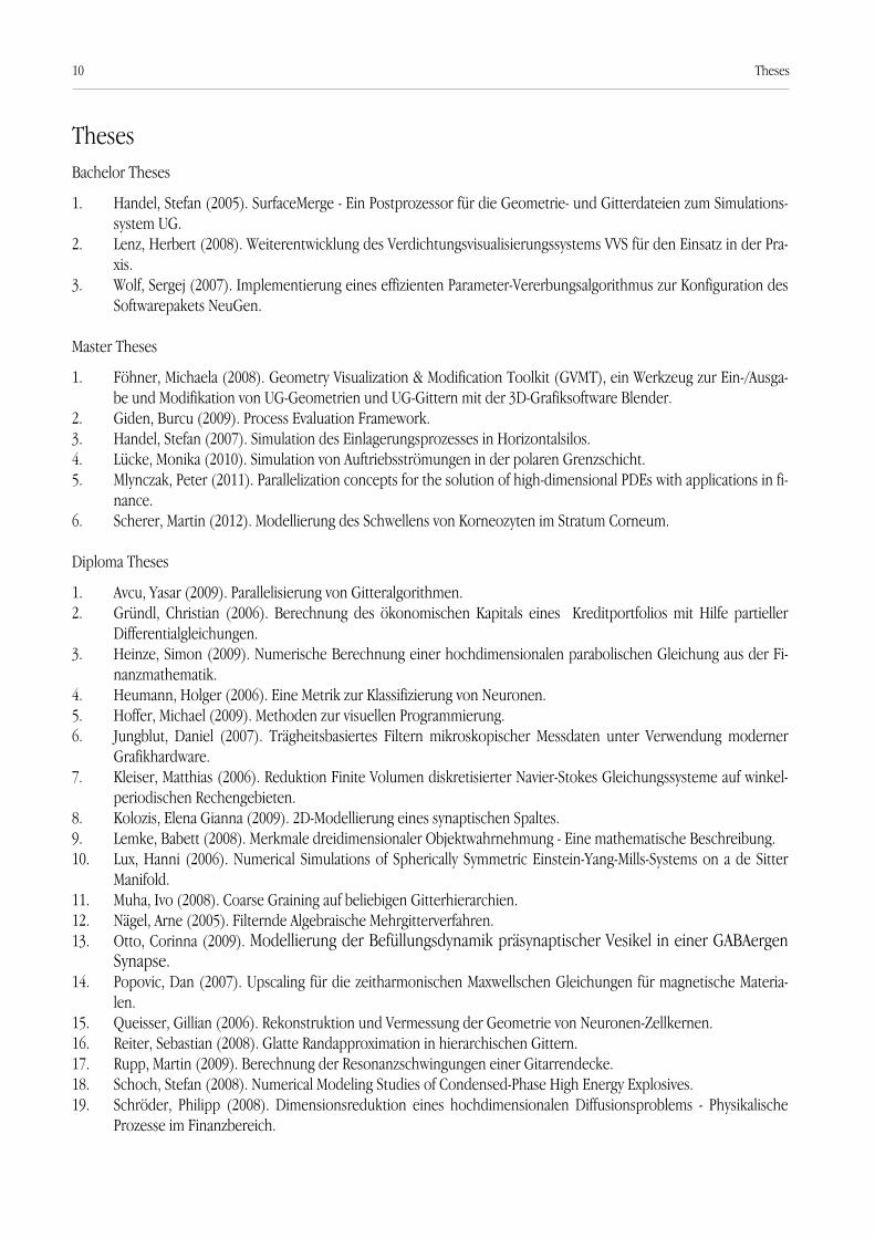
ThesesBachelor Theses

1. Handel, Stefan (2005). SurfaceMerge - Ein Postprozessor für die Geometrie- und Gitterdateien zum Simulations-system UG.

2. Lenz, Herbert (2008). Weiterentwicklung des Verdichtungsvisualisierungssystems VVS für den Einsatz in der Pra-xis.

3. Wolf, Sergej (2007). Implementierung eines effizienten Parameter-Vererbungsalgorithmus zur Konfiguration desSoftwarepakets NeuGen.

Master Theses

1. Föhner, Michaela (2008). Geometry Visualization & Modification Toolkit (GVMT), ein Werkzeug zur Ein-/Ausga-be und Modifikation von UG-Geometrien und UG-Gittern mit der 3D-Grafiksoftware Blender.

2. Giden, Burcu (2009). Process Evaluation Framework.3. Handel, Stefan (2007). Simulation des Einlagerungsprozesses in Horizontalsilos.4. Lücke, Monika (2010). Simulation von Auftriebsströmungen in der polaren Grenzschicht.5. Mlynczak, Peter (2011). Parallelization concepts for the solution of high-dimensional PDEs with applications in fi-

nance.6. Scherer, Martin (2012). Modellierung des Schwellens von Korneozyten im Stratum Corneum.

Diploma Theses

1. Avcu, Yasar (2009). Parallelisierung von Gitteralgorithmen.2. Gründl, Christian (2006). Berechnung des ökonomischen Kapitals eines Kreditportfolios mit Hilfe partieller

Differentialgleichungen.3. Heinze, Simon (2009). Numerische Berechnung einer hochdimensionalen parabolischen Gleichung aus der Fi-

nanzmathematik.4. Heumann, Holger (2006). Eine Metrik zur Klassifizierung von Neuronen.5. Hoffer, Michael (2009). Methoden zur visuellen Programmierung.6. Jungblut, Daniel (2007). Trägheitsbasiertes Filtern mikroskopischer Messdaten unter Verwendung moderner

Grafikhardware.7. Kleiser, Matthias (2006). Reduktion Finite Volumen diskretisierter Navier-Stokes Gleichungssysteme auf winkel-

periodischen Rechengebieten.8. Kolozis, Elena Gianna (2009). 2D-Modellierung eines synaptischen Spaltes.9. Lemke, Babett (2008). Merkmale dreidimensionaler Objektwahrnehmung - Eine mathematische Beschreibung.10. Lux, Hanni (2006). Numerical Simulations of Spherically Symmetric Einstein-Yang-Mills-Systems on a de Sitter

Manifold.11. Muha, Ivo (2008). Coarse Graining auf beliebigen Gitterhierarchien.12. Nägel, Arne (2005). Filternde Algebraische Mehrgitterverfahren.13. Otto, Corinna (2009). Modellierung der Befüllungsdynamik präsynaptischer Vesikel in einer GABAergen

Synapse.14. Popovic, Dan (2007). Upscaling für die zeitharmonischen Maxwellschen Gleichungen für magnetische Materia-

len.15. Queisser, Gillian (2006). Rekonstruktion und Vermessung der Geometrie von Neuronen-Zellkernen.16. Reiter, Sebastian (2008). Glatte Randapproximation in hierarchischen Gittern.17. Rupp, Martin (2009). Berechnung der Resonanzschwingungen einer Gitarrendecke.18. Schoch, Stefan (2008). Numerical Modeling Studies of Condensed-Phase High Energy Explosives.19. Schröder, Philipp (2008). Dimensionsreduktion eines hochdimensionalen Diffusionsproblems - Physikalische

Prozesse im Finanzbereich.

10 Theses

20. Stichel, Sabine (2008). Numerisches Coarse Graining in UG.21. Urbahn, Ulrich (2008). Entwicklung eines Ratingverfahrens für Versicherungen.22. Vogel, Andreas (2008). Ein Finite-Volumen-Verfahren höherer Ordnung mit Anwendung in der Biophysik.23. Voßen, Christine (2006). Passive Signalleitung in Nervenzellen.24. Wahner, Ralf (2005). Complex Layered Domain Modeller - Ein 3D Gitter- und Geometriegenerator für das Nu-

meriksimulationssystem UG.25. Wehner, Christian (2007). Numerische Verfahren für Transportgleichungen unter Verwendung von Level-Set-

Verfahren.26. Wanner, Alexander (2007). Ein effizientes Verfahren zur Berechnung der Potentiale in kortikalen neuronalen Ko-

lumnen.27. Xylouris, Konstantinos (2008). Signalverarbeitung in Neuronen.

PhD Theses

1. Feuchter, Dirk (2008). Geometrie- und Gittererzeugung für anisotrope Schichtengebiete.2. Hauser, Andreas (2009). Large Eddy Simulation auf uniform und adaptiv verfeinerten Gittern.3. Jungblut, Daniel (2010). Rekonstruktion von Oberflächenmorphologien und Merkmalskeletten aus dreidimensi-

onalen Daten unter Verwendung hochparalleler Rechnerarchitekturen.4. Kicherer, Walter (2007). Objektorientierte Programmierung in der Schule.5 Lampe, Michael (2006). Parallele Visualisierung – Ein Vergleich.6. Nägel, Arne (2009). Schnelle Löser für große Gleichungssysteme mit Anwendungen in der Biophysik und den

Lebenswissenschaften.7. Queisser, Gillian (2008). The Influence of the Morphology of Nuclei from Hippocampal Neurons on Signal Pro-

cessing in Nuclei.8. Schröder, Philipp (2011). Dimensionsweise Zerlegungen hochdimensionaler Probleme mit Anwendungen im Fi-

nanzbereich.

Awards• 1st price of the doIT-Software-Award, 2005• Poster award at OEESC 2007

Academic Offers to G-CSC(SiM)/SiT Members

• Wittum, Gabriel, FU Berlin, 2005 (W3)• Johannsen, Klaus, German University Kairo, 2006 (Full Professorship)• Johannsen, Klaus, Universitetet i Bergen, 2006 • Wittum, Gabriel, U Paderborn 2006 (W3)• Wittum, Gabriel, U Laramie 2007 (Distinguished Professorship)• Wittum, Gabriel, U Frankfurt 2007• Queisser, Gillian, U Frankfurt 2009• Reichenberger, Volker, European Business School, Reutlingen, 2010

Theses 11

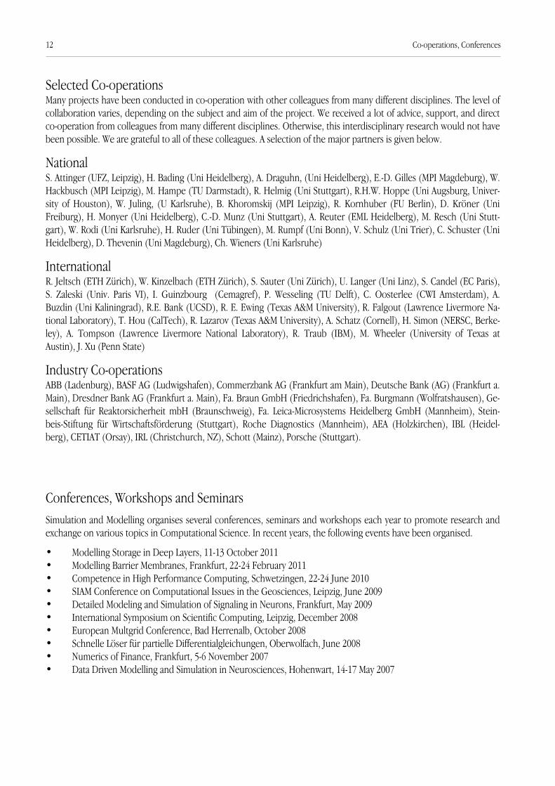
Selected Co-operationsMany projects have been conducted in co-operation with other colleagues from many different disciplines. The level ofcollaboration varies, depending on the subject and aim of the project. We received a lot of advice, support, and directco-operation from colleagues from many different disciplines. Otherwise, this interdisciplinary research would not havebeen possible. We are grateful to all of these colleagues. A selection of the major partners is given below.

NationalS. Attinger (UFZ, Leipzig), H. Bading (Uni Heidelberg), A. Draguhn, (Uni Heidelberg), E.-D. Gilles (MPI Magdeburg), W.Hackbusch (MPI Leipzig), M. Hampe (TU Darmstadt), R. Helmig (Uni Stuttgart), R.H.W. Hoppe (Uni Augsburg, Univer-sity of Houston), W. Juling, (U Karlsruhe), B. Khoromskij (MPI Leipzig), R. Kornhuber (FU Berlin), D. Kröner (UniFreiburg), H. Monyer (Uni Heidelberg), C.-D. Munz (Uni Stuttgart), A. Reuter (EML Heidelberg), M. Resch (Uni Stutt-gart), W. Rodi (Uni Karlsruhe), H. Ruder (Uni Tübingen), M. Rumpf (Uni Bonn), V. Schulz (Uni Trier), C. Schuster (UniHeidelberg), D. Thevenin (Uni Magdeburg), Ch. Wieners (Uni Karlsruhe)

InternationalR. Jeltsch (ETH Zürich), W. Kinzelbach (ETH Zürich), S. Sauter (Uni Zürich), U. Langer (Uni Linz), S. Candel (EC Paris),S. Zaleski (Univ. Paris VI), I. Guinzbourg (Cemagref), P. Wesseling (TU Delft), C. Oosterlee (CWI Amsterdam), A.Buzdin (Uni Kaliningrad), R.E. Bank (UCSD), R. E. Ewing (Texas A&M University), R. Falgout (Lawrence Livermore Na-tional Laboratory), T. Hou (CalTech), R. Lazarov (Texas A&M University), A. Schatz (Cornell), H. Simon (NERSC, Berke-ley), A. Tompson (Lawrence Livermore National Laboratory), R. Traub (IBM), M. Wheeler (University of Texas atAustin), J. Xu (Penn State)

Industry Co-operationsABB (Ladenburg), BASF AG (Ludwigshafen), Commerzbank AG (Frankfurt am Main), Deutsche Bank (AG) (Frankfurt a.Main), Dresdner Bank AG (Frankfurt a. Main), Fa. Braun GmbH (Friedrichshafen), Fa. Burgmann (Wolfratshausen), Ge-sellschaft für Reaktorsicherheit mbH (Braunschweig), Fa. Leica-Microsystems Heidelberg GmbH (Mannheim), Stein-beis-Stiftung für Wirtschaftsförderung (Stuttgart), Roche Diagnostics (Mannheim), AEA (Holzkirchen), IBL (Heidel-berg), CETIAT (Orsay), IRL (Christchurch, NZ), Schott (Mainz), Porsche (Stuttgart).

Conferences, Workshops and SeminarsSimulation and Modelling organises several conferences, seminars and workshops each year to promote research andexchange on various topics in Computational Science. In recent years, the following events have been organised.

• Modelling Storage in Deep Layers, 11-13 October 2011• Modelling Barrier Membranes, Frankfurt, 22-24 February 2011• Competence in High Performance Computing, Schwetzingen, 22-24 June 2010• SIAM Conference on Computational Issues in the Geosciences, Leipzig, June 2009• Detailed Modeling and Simulation of Signaling in Neurons, Frankfurt, May 2009• International Symposium on Scientific Computing, Leipzig, December 2008• European Multgrid Conference, Bad Herrenalb, October 2008• Schnelle Löser für partielle Differentialgleichungen, Oberwolfach, June 2008• Numerics of Finance, Frankfurt, 5-6 November 2007• Data Driven Modelling and Simulation in Neurosciences, Hohenwart, 14-17 May 2007

12 Co-operations, Conferences

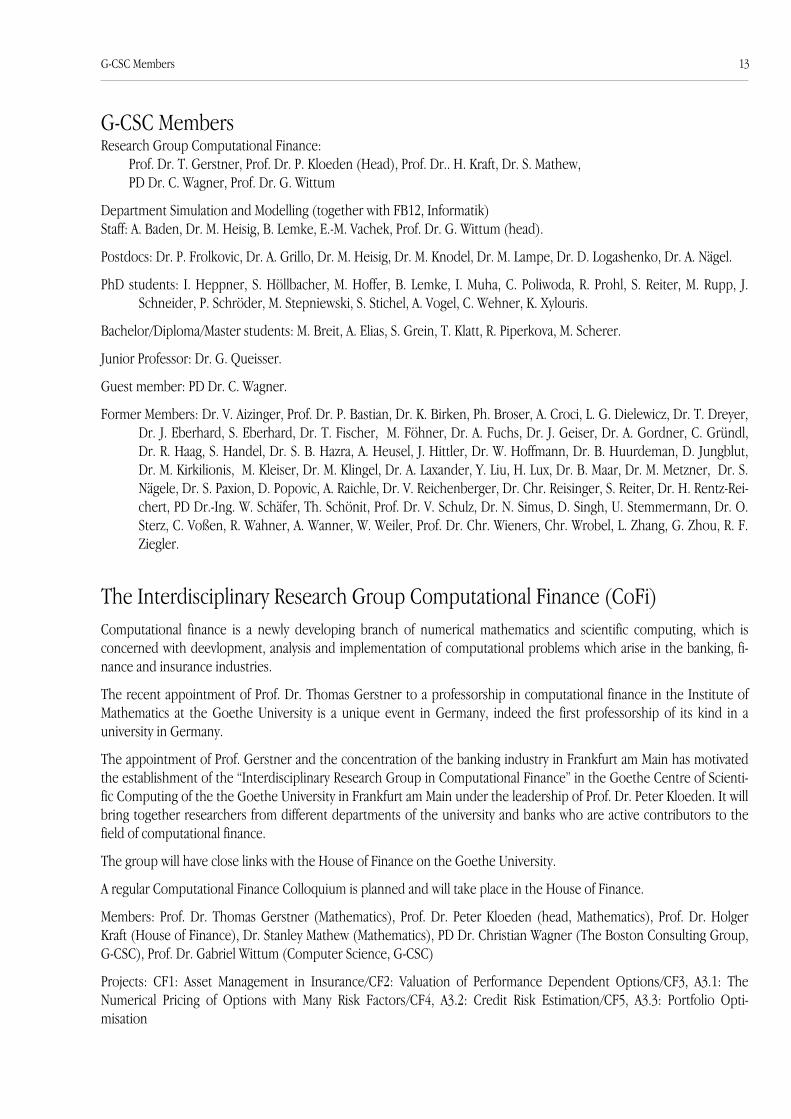
G-CSC MembersResearch Group Computational Finance:

Prof. Dr. T. Gerstner, Prof. Dr. P. Kloeden (Head), Prof. Dr.. H. Kraft, Dr. S. Mathew,PD Dr. C. Wagner, Prof. Dr. G. Wittum

Department Simulation and Modelling (together with FB12, Informatik)Staff: A. Baden, Dr. M. Heisig, B. Lemke, E.-M. Vachek, Prof. Dr. G. Wittum (head).

Postdocs: Dr. P. Frolkovic, Dr. A. Grillo, Dr. M. Heisig, Dr. M. Knodel, Dr. M. Lampe, Dr. D. Logashenko, Dr. A. Nägel.

PhD students: I. Heppner, S. Höllbacher, M. Hoffer, B. Lemke, I. Muha, C. Poliwoda, R. Prohl, S. Reiter, M. Rupp, J.Schneider, P. Schröder, M. Stepniewski, S. Stichel, A. Vogel, C. Wehner, K. Xylouris.

Bachelor/Diploma/Master students: M. Breit, A. Elias, S. Grein, T. Klatt, R. Piperkova, M. Scherer.

Junior Professor: Dr. G. Queisser.

Guest member: PD Dr. C. Wagner.

Former Members: Dr. V. Aizinger, Prof. Dr. P. Bastian, Dr. K. Birken, Ph. Broser, A. Croci, L. G. Dielewicz, Dr. T. Dreyer,Dr. J. Eberhard, S. Eberhard, Dr. T. Fischer, M. Föhner, Dr. A. Fuchs, Dr. J. Geiser, Dr. A. Gordner, C. Gründl,Dr. R. Haag, S. Handel, Dr. S. B. Hazra, A. Heusel, J. Hittler, Dr. W. Hoffmann, Dr. B. Huurdeman, D. Jungblut,Dr. M. Kirkilionis, M. Kleiser, Dr. M. Klingel, Dr. A. Laxander, Y. Liu, H. Lux, Dr. B. Maar, Dr. M. Metzner, Dr. S.Nägele, Dr. S. Paxion, D. Popovic, A. Raichle, Dr. V. Reichenberger, Dr. Chr. Reisinger, S. Reiter, Dr. H. Rentz-Rei-chert, PD Dr.-Ing. W. Schäfer, Th. Schönit, Prof. Dr. V. Schulz, Dr. N. Simus, D. Singh, U. Stemmermann, Dr. O.Sterz, C. Voßen, R. Wahner, A. Wanner, W. Weiler, Prof. Dr. Chr. Wieners, Chr. Wrobel, L. Zhang, G. Zhou, R. F.Ziegler.

The Interdisciplinary Research Group Computational Finance (CoFi)Computational finance is a newly developing branch of numerical mathematics and scientific computing, which isconcerned with deevlopment, analysis and implementation of computational problems which arise in the banking, fi-nance and insurance industries.

The recent appointment of Prof. Dr. Thomas Gerstner to a professorship in computational finance in the Institute ofMathematics at the Goethe University is a unique event in Germany, indeed the first professorship of its kind in auniversity in Germany.

The appointment of Prof. Gerstner and the concentration of the banking industry in Frankfurt am Main has motivatedthe establishment of the “Interdisciplinary Research Group in Computational Finance” in the Goethe Centre of Scienti-fic Computing of the the Goethe University in Frankfurt am Main under the leadership of Prof. Dr. Peter Kloeden. It willbring together researchers from different departments of the university and banks who are active contributors to thefield of computational finance.

The group will have close links with the House of Finance on the Goethe University.

A regular Computational Finance Colloquium is planned and will take place in the House of Finance.

Members: Prof. Dr. Thomas Gerstner (Mathematics), Prof. Dr. Peter Kloeden (head, Mathematics), Prof. Dr. HolgerKraft (House of Finance), Dr. Stanley Mathew (Mathematics), PD Dr. Christian Wagner (The Boston Consulting Group,G-CSC), Prof. Dr. Gabriel Wittum (Computer Science, G-CSC)

Projects: CF1: Asset Management in Insurance/CF2: Valuation of Performance Dependent Options/CF3, A3.1: TheNumerical Pricing of Options with Many Risk Factors/CF4, A3.2: Credit Risk Estimation/CF5, A3.3: Portfolio Opti-misation

G-CSC Members 13

A1: Modelling Barrier MembranesArne Nägel, Dirk Feuchter, Michael Heisig, Christine Wagner, Gabriel Wittum

The investigation of barrier membranes is important in various fields of engineering and life sciences. For many in-dustrial applications, notably in food packaging, coatings and chemical separations, the study of chemical diffusionand transport of substances is of great significance. Closely linked transport through biological barrier membranesplays a vital role in pharmaceutical research and development. This is true not only for clinical studies where drugs

are applied in different epithelia barrier membranes (e.g., intesti-ne, lung, blood-brain barrier, skin) but also for the risk assess-ment of substances in various exposure scenarios. Until now in-vitro test systems are used to give some information about thein-vivo situation and replace animal experiments. In order to in-crease capacity, speed, and cost-effectiveness of such studies sig-nificantly, in-silico test systems with an adequate predictive po-wer have to be developed. As an archetypical example of a biolo-gical barrier membrane we have investigated the diffusion ofdrugs through skin by numerical simulation.

The barrier function of mammalian skin is primarily located inthe outermost epidermal layer, the stratum corneum (SC). Thismorphological unit consists of dead, flattened, keratinised cells,the corneocytes, which are embedded in a contiguous layer of li-pid (Figure 1). Investigations of the stratum corneum are ham-pered by enormous difficulties regarding equipment and experi-ments. This is the reason, why the physical properties of thisskin layer have hitherto been grasped insufficiently. The numeri-cal simulation of drug diffusion through the stratum corneumcontributes to understanding of the permeation process.

In a simulation with high resolution of geometric details, the ma-thematical challenge first of all comes from the complicatedstructure. This leads to a large number of degrees of freedom.

Secondly the associated bio-physical properties induce discontinuities which makes the use of robust multigrid me-thods mandatory.

This project began with the development of a two-dimensional model for the diffusion of xenobiotics through thehuman stratum corneum (Heisig et al. 1996). In this model, we showed that, in addition to the commonly cited lipidmultilamellar pathway, intracorneocytediffusion must exist to match the experi-mental data. Ten years later this was con-firmed experimentally using dual-channelhigh-speed two-photon fluorescence mi-croscopy (Yu et al. 2003). Since these firststeps, the model has been refined in va-rious aspects:

In cooperation with researchers from theSaarland University the development of avirtual skin model has been addressed. Inthis context the geometry has been exten-ded by an additional compartment for thedeeper skin layers (DSL). An illustration is

Figure 1. Micrographs of cross-sections of mouseskin (6) and mouse stratum corneum (7,8) (fromMenton, 1976)

hDSL = 1.5 mm Deeper skin layers, !DSL

Lipid layers, lip

Lcor= 30"m

# = 0.1 "m

hcor = 1.0 "m $cor,lip

$DSL,lip

$in

$ DS

L,si

de

$out

$ lip

,sid

e$ c

or,s

ide

%

Corneocytes, cor

!

!

Figure 2. 2D model of the stratum corneum and deeper skin layers (fromNaegel et al. 2008)

14 A1: Modelling Barrier Membranes

shown in Figure 2. All phases are modelled with homo-geneous diffusivity. Lipid-donor and SC–DSL partitioncoefficients are determined experimentally, while corne-ocyte–lipid and DSL–lipid partition coefficients are deri-ved consistently with the model. Together with experi-mentally determined apparent lipid- and DSL-diffusioncoefficients, these data serve as direct input for compu-tational modelling of drug transport through the skin.The apparent corneocyte diffusivity is estimated basedon an approximation, which uses the apparent SC- andlipid-diffusion coefficients as well as corneocyte–lipidpartition coefficients. The quality of the model is evalua-

ted by a comparison of concentration–SC-depth pro-files of the experiment with those of the simulation.For two representative test compounds, flufenamicacid (lipophilic) and caffeine (hydrophilic) good ag-reements between experiment and simulation areobtained (Hansen et al. 2008; Naegel et al. 2008; Nä-gel 2009b; Naegel et al. 2011) which is shown for caf-feine in Figure 3. Moreover the results providedhints, that additional processes, such as keratine bin-ding, were also important to consider. The role ofthis particular effect was then studied numerically,

before an appropriate experimental design was developed (Hansen et al. 2009).

With respect to geometry, several cellular models in both two and three space dimensions are supported now.The most elaborate and most flexible cell model is based on Kelvin's tetrakaidekahedron (TKD). This 14-faced struc-ture features a realistic structure and surface-to-volume ratio and may therefore serve as a general building block forcellular membranes (Feuchter et al. 2006; Feuchter 2008). An example for a stratum corneum membrane consistingof ten cell layers is shown in Figure 4. Simpler models are based, e.g., on cuboids (Wagner 2008). In Figures 5 and 6time-dependent concentration profiles within tetrakaidekahedral and cuboidal model membranes are shown.

The barrier property of a membrane is described by two parameters: the permeability and the lag time. Using nume-rical simulation the influence of the cell geometry on the permeability and lag time of two- and three-dimensionalmembranes has been studied (Naegel et al. 2009a; Nägel 2009b; Naegel et al. 2011). In Figure 7, the relative permea-

6h2h

Simulation: 1h6h2h

Experiment: 1h

rel. SC depth

Ca!e

ineconc

entration[µ

g/ml]

10.80.60.40.20

60000

50000

40000

30000

20000

10000

0

Figure 3. Concentration-depth profile for caffeine (from Nae-gel et al. 2008)

Figure 4. Tetrakaidekahedralmodel stratum corneum(cross section)

Figure 6. Evolution of concentration in cuboid 3D model (from Wagner 2008)

Figure 5. Evolution of concentration in tetrakaidekahedral model stratum corneum (from Nägel et al. 2006).

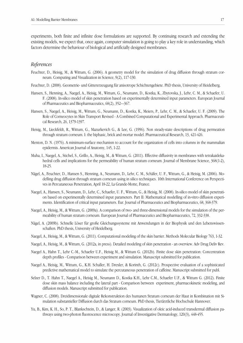
A1: Modelling Barrier Membranes 15

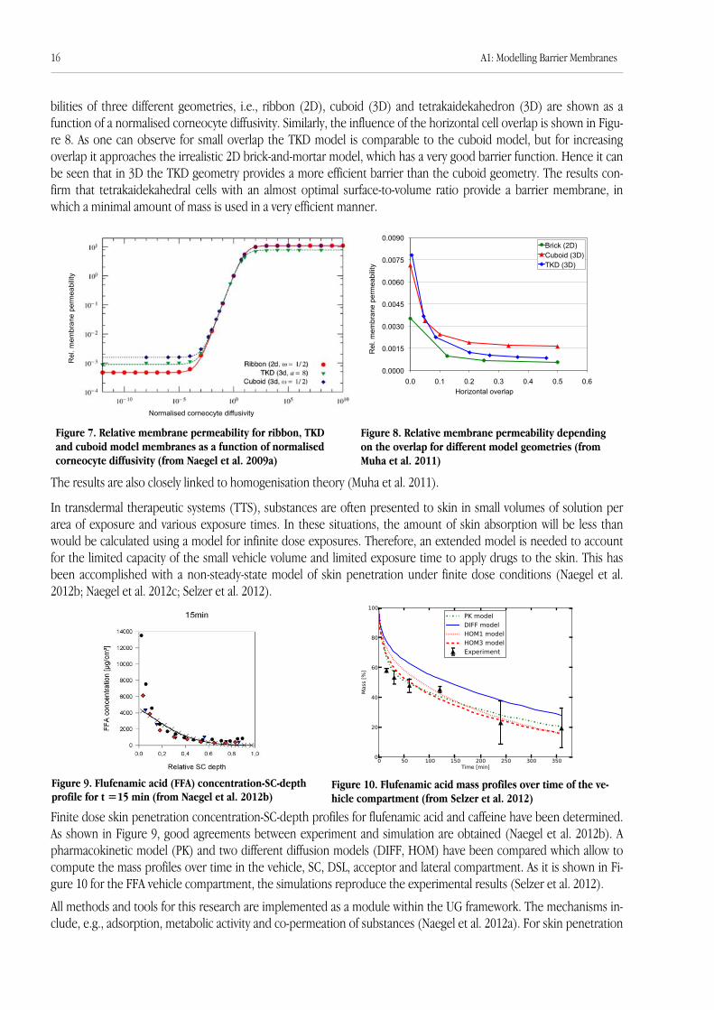
bilities of three different geometries, i.e., ribbon (2D), cuboid (3D) and tetrakaidekahedron (3D) are shown as afunction of a normalised corneocyte diffusivity. Similarly, the influence of the horizontal cell overlap is shown in Figu-re 8. As one can observe for small overlap the TKD model is comparable to the cuboid model, but for increasingoverlap it approaches the irrealistic 2D brick-and-mortar model, which has a very good barrier function. Hence it canbe seen that in 3D the TKD geometry provides a more efficient barrier than the cuboid geometry. The results con-firm that tetrakaidekahedral cells with an almost optimal surface-to-volume ratio provide a barrier membrane, inwhich a minimal amount of mass is used in a very efficient manner.

The results are also closely linked to homogenisation theory (Muha et al. 2011).

In transdermal therapeutic systems (TTS), substances are often presented to skin in small volumes of solution perarea of exposure and various exposure times. In these situations, the amount of skin absorption will be less thanwould be calculated using a model for infinite dose exposures. Therefore, an extended model is needed to accountfor the limited capacity of the small vehicle volume and limited exposure time to apply drugs to the skin. This hasbeen accomplished with a non-steady-state model of skin penetration under finite dose conditions (Naegel et al.2012b; Naegel et al. 2012c; Selzer et al. 2012).

Finite dose skin penetration concentration-SC-depth profiles for flufenamic acid and caffeine have been determined.As shown in Figure 9, good agreements between experiment and simulation are obtained (Naegel et al. 2012b). Apharmacokinetic model (PK) and two different diffusion models (DIFF, HOM) have been compared which allow tocompute the mass profiles over time in the vehicle, SC, DSL, acceptor and lateral compartment. As it is shown in Fi-gure 10 for the FFA vehicle compartment, the simulations reproduce the experimental results (Selzer et al. 2012).

All methods and tools for this research are implemented as a module within the UG framework. The mechanisms in-clude, e.g., adsorption, metabolic activity and co-permeation of substances (Naegel et al. 2012a). For skin penetration

Figure 9. Flufenamic acid (FFA) concentration-SC-depthprofile for t =15 min (from Naegel et al. 2012b)

16 A1: Modelling Barrier Membranes

Figure 10. Flufenamic acid mass profiles over time of the ve-hicle compartment (from Selzer et al. 2012)

Figure 8. Relative membrane permeability dependingon the overlap for different model geometries (fromMuha et al. 2011)

0.0000

0.0015

0.0030

0.0045

0.0060

0.0075

0.0090

0.0 0.1 0.2 0.3 0.4 0.5 0.6

Brick (2D) Cuboid (3D) TKD (3D)

Horizontal overlap

Rel

. mem

bran

e pe

rmea

bilit

y

Normalised corneocyte diffusivity

Rel

. mem

bran

e pe

rmea

bilit

y

Figure 7. Relative membrane permeability for ribbon, TKDand cuboid model membranes as a function of normalisedcorneocyte diffusivity (from Naegel et al. 2009a)

experiments, both finite and infinite dose formulations are supported. By continuing research and extending theexisting models, we expect that, once again, computer simulation is going to play a key role in understanding, whichfactors determine the behaviour of biological and artificially designed membranes.

ReferencesFeuchter, D., Heisig, M., & Wittum, G. (2006). A geometry model for the simulation of drug diffusion through stratum cor-

neum. Computing and Visualization in Science, 9(2), 117-130.

Feuchter, D. (2008). Geometrie- und Gittererzeugung für anisotrope Schichtengebiete. PhD thesis, University of Heidelberg.

Hansen, S., Henning, A., Naegel, A., Heisig, M., Wittum, G., Neumann, D., Kostka, K., Zbytovska, J., Lehr, C. M., & Schaefer, U.F. (2008). In-silico model of skin penetration based on experimentally determined input parameters. European Journalof Pharmaceutics and Biopharmaceutics, 68(2), 352–-367.

Hansen, S., Naegel, A., Heisig, M., Wittum, G., Neumann, D., Kostka, K., Meiers, P., Lehr, C. M., & Schaefer, U. F. (2009). TheRole of Corneocytes in Skin Transport Revised - A Combined Computational and Experimental Approach. Pharmaceuti-cal Research, 26, 1379-1397.

Heisig, M., Lieckfeldt, R., Wittum, G., Mazurkevich G., & Lee, G. (1996). Non steady-state descriptions of drug permeationthrough stratum corneum. I: the biphasic, brick and mortar model. Pharmaceutical Research, 13, 421-426.

Menton, D. N. (1976). A minimum-surface mechanism to account for the organization of cells into columns in the mammalianepidermis. American Journal of Anatomy, 145, 1-22.

Muha, I., Naegel, A., Stichel, S., Grillo, A., Heisig, M., & Wittum, G. (2011). Effective diffusivity in membranes with tetrakaideka-hedral cells and implications for the permeability of human stratum corneum. Journal of Membrane Science, 368(1-2),18-25.

Nägel, A., Feuchter, D., Hansen S., Henning, A., Neumann, D., Lehr, C. M., Schäfer, U. F., Wittum, G., & Heisig, M. (2006). Mo-delling drug diffusion through stratum corneum using in silico techniques. 10th International Conference on Perspecti-ves in Percutaneous Penetration, April 18-22, La Grande-Motte, France.

Naegel, A., Hansen, S., Neumann, D., Lehr, C., Schaefer, U. F., Wittum, G., & Heisig, M. (2008). In-silico model of skin penetrati-on based on experimentally determined input parameters. Part II: Mathematical modelling of in-vitro diffusion experi-ments. Identification of critical input parameters. Eur. Journal of Pharmaceutics and Biopharmaceutics, 68, 368-379.

Naegel, A., Heisig, M., & Wittum, G. (2009a). A comparison of two- and three-dimensional models for the simulation of the per-meability of human stratum corneum. European Journal of Pharmaceutics and Biopharmaceutics, 72, 332-338.

Nägel, A. (2009b). Schnelle Löser für große Gleichungssysteme mit Anwendungen in der Biophysik und den Lebenswissen-schaften. PhD thesis, University of Heidelberg.

Naegel, A., Heisig, M., & Wittum, G. (2011). Computational modeling of the skin barrier. Methods Molecular Biology 763, 1-32.

Naegel, A., Heisig, M., & Wittum, G. (2012a, in press). Detailed modeling of skin penetration - an overview. Adv Drug Deliv Rev.

Naegel A., Hahn T., Lehr C.-M., Schaefer U.F., Heisig M., & Wittum G. (2012b). Finite dose skin penetration: Concentrationdepth profiles - Comparison between experiment and simulation. Manuscript submitted for publication.

Naegel A., Heisig, M., Wittum, G., K.H. Schaller, H. Drexler, & Korinth, G. (2012c). Prospective evaluation of a sophisticatedpredictive mathematical model to simulate the percutaneous penetration of caffeine. Manuscript submitted for publ.

Selzer D., T. Hahn T., Naegel A., Heisig M., Neumann D., Kostka K.H., Lehr C.M., Schaefer U.F., & Wittum G. (2012). Finitedose skin mass balance including the lateral part - Comparison between experiment, pharmacokinetic modeling, anddiffusion models. Manuscript submitted for publication.

Wagner, C. (2008). Dreidimensionale digitale Rekonstruktion des humanen Stratum corneum der Haut in Kombination mit Si-mulation substantieller Diffusion durch das Stratum corneum. PhD thesis, Tierärztliche Hochschule Hannover.

Yu, B., Kim, K. H., So, P. T., Blankschtein, D., & Langer, R. (2003). Visualization of oleic acid-induced transdermal diffusion pa-thways using two-photon fluorescence microscopy. Journal of Investigative Dermatology, 120(3), 448-455.

A1: Modelling Barrier Membranes 17

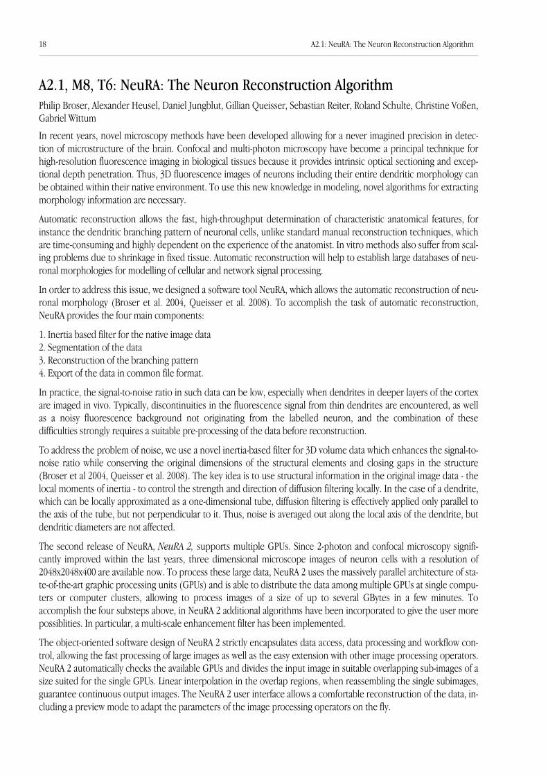
A2.1, M8, T6: NeuRA: The Neuron Reconstruction Algorithm Philip Broser, Alexander Heusel, Daniel Jungblut, Gillian Queisser, Sebastian Reiter, Roland Schulte, Christine Voßen,Gabriel Wittum

In recent years, novel microscopy methods have been developed allowing for a never imagined precision in detec-tion of microstructure of the brain. Confocal and multi-photon microscopy have become a principal technique forhigh-resolution fluorescence imaging in biological tissues because it provides intrinsic optical sectioning and excep-tional depth penetration. Thus, 3D fluorescence images of neurons including their entire dendritic morphology canbe obtained within their native environment. To use this new knowledge in modeling, novel algorithms for extractingmorphology information are necessary.

Automatic reconstruction allows the fast, high-throughput determination of characteristic anatomical features, forinstance the dendritic branching pattern of neuronal cells, unlike standard manual reconstruction techniques, whichare time-consuming and highly dependent on the experience of the anatomist. In vitro methods also suffer from scal-ing problems due to shrinkage in fixed tissue. Automatic reconstruction will help to establish large databases of neu-ronal morphologies for modelling of cellular and network signal processing.

In order to address this issue, we designed a software tool NeuRA, which allows the automatic reconstruction of neu-ronal morphology (Broser et al. 2004, Queisser et al. 2008). To accomplish the task of automatic reconstruction,NeuRA provides the four main components:

1. Inertia based filter for the native image data2. Segmentation of the data3. Reconstruction of the branching pattern4. Export of the data in common file format.

In practice, the signal-to-noise ratio in such data can be low, especially when dendrites in deeper layers of the cortexare imaged in vivo. Typically, discontinuities in the fluorescence signal from thin dendrites are encountered, as wellas a noisy fluorescence background not originating from the labelled neuron, and the combination of thesedifficulties strongly requires a suitable pre-processing of the data before reconstruction.

To address the problem of noise, we use a novel inertia-based filter for 3D volume data which enhances the signal-to-noise ratio while conserving the original dimensions of the structural elements and closing gaps in the structure(Broser et al 2004, Queisser et al. 2008). The key idea is to use structural information in the original image data - thelocal moments of inertia - to control the strength and direction of diffusion filtering locally. In the case of a dendrite,which can be locally approximated as a one-dimensional tube, diffusion filtering is effectively applied only parallel tothe axis of the tube, but not perpendicular to it. Thus, noise is averaged out along the local axis of the dendrite, butdendritic diameters are not affected.

The second release of NeuRA, NeuRA 2, supports multiple GPUs. Since 2-photon and confocal microscopy signifi-cantly improved within the last years, three dimensional microscope images of neuron cells with a resolution of2048x2048x400 are available now. To process these large data, NeuRA 2 uses the massively parallel architecture of sta-te-of-the-art graphic processing units (GPUs) and is able to distribute the data among multiple GPUs at single compu-ters or computer clusters, allowing to process images of a size of up to several GBytes in a few minutes. Toaccomplish the four substeps above, in NeuRA 2 additional algorithms have been incorporated to give the user morepossiblities. In particular, a multi-scale enhancement filter has been implemented.

The object-oriented software design of NeuRA 2 strictly encapsulates data access, data processing and workflow con-trol, allowing the fast processing of large images as well as the easy extension with other image processing operators.NeuRA 2 automatically checks the available GPUs and divides the input image in suitable overlapping sub-images of asize suited for the single GPUs. Linear interpolation in the overlap regions, when reassembling the single subimages,guarantee continuous output images. The NeuRA 2 user interface allows a comfortable reconstruction of the data, in-cluding a preview mode to adapt the parameters of the image processing operators on the fly.

18 A2.1: NeuRA: The Neuron Reconstruction Algorithm

Using general noice reduction and segmentation methods rather than model-based techniques, NeuRA 2 is not limi-ted to reconstruct neuron cells (Figure 1). It can also be used to generate surface meshes from archaeological (Figu-re 5; Jungblut et al. 2009b) or medical computer tomography images (Figure 6), as well as nuclei (Queisser et al.2008) or other neurobiological microscopy images, like presynaptic boutons (Figure 2) or dendrite segments withspines (Figure 3).

References

Broser, P. J., Schulte, R., Roth, A., Helmchen, F., Waters, J., Lang, S., Sakmann, B., & Wittum, G. (2004). Nonlinearanisotropic diffusion filtering of three-dimensional image data from 2-photon microscopy. Journal ofBiomedical Optics, 9(6), 1253–1264.

Jungblut, D., Queisser, G., & Wittum, G. (2012). Inertia Based Filtering of High Resolution Images Using a GPUCluster. Computing and Visualization in Science, 14(4), 181-186.

Jungblut, D., Karl, S., Mara, H., Krömker, S., & Wittum, G. (2009). Automated GPU-based Surface Morphology Recon-struction of Volume Data for Archeology. SCCH 2009.

Queisser, G., Bading, H., Wittmann, M., & Wittum, G. (2008). Filtering, reconstruction, and measurement of the geo-metry of nuclei from hippocampal neurons based on confocal microscopy data. Journal of Biomedical Optics,13(1), 014009.

A2.1: NeuRA: The Neuron Reconstruction Algorithm 19

Figure 5. Reconstruction of a ceramic vase Figure 6. Reconstruction of a cervical spine

Figure 1. Reconstruction of a neuroncell (data from Jakob v. Engelhardt,Hannah Monyer)

Figure 2. Presynaptic bouton Figure(data from Daniel Bucher, ChristophSchuster)

Figure 3. Dendrite segment with spines(data from Andreas Vlachos, ThomasDeller)

A2.2: Modelling the Nuclear Calcium CodeGillian Queisser, Gabriel Wittum

Calcium regulates virtually all cellular responses in the mammalian brain. Many biochemical processes in the cellinvolved in learning, memory formation as well as cell survival and death, are regulated by calcium (Bading 2000,Milner 1998, West 2002). Especially when investigating neurodegenerative deseases like Alzheimer‘s or Parkinson‘sdisease the calcium code plays a central role. Signalling from synapses to nucleus through calcium waves and thesubsequent relay of information to the nucleus that activates transcriptional events was of special interest in a projecttogether with the Bading lab at the IZN in Heidelberg.

Electron microscopy studies in hippocampal rat tissue carried out at the lab revealed novel features of the nuclearmembrane morphology (Wittmann et al., 2009). While current text book depictions show the nucleus to have aspherical form, these electron micrographs showed infolded membrane formations of both nuclear membranes (Fi-gure 1, left).

To assess the realistic morphologies of hippocampal nuclei and to investigate the influence of the diverse structureson nuclear calcium signalling, we used NeuRA (Queisser et al. 2008) to reconstruct the nuclear membrane surfacefrom confocal microscopy recordings (Figure 1, right). As a first result one could ascertain, that the hippocampal areacontains a large quantity of highly infolded nuclei, where the nuclear envelope divides nuclei into microdomains.Furthermore, measuring surface and volume of infolded and spherical nuclei showed that all nuclei are nearly equalin their volume but infolded nuclei have an approx. 20% larger surface than spherical ones (Wittmann et al., 2009).This surface increase is proportional to the increase in nuclear pore complexes (NPCs) on the membrane throughwhich cytosol can freely diffuse into the nucleus. This observation, and the visible compartimentalisation of nucleiled us to investigate the morphological effect on nuclear calcium signalling.

Therefore we developed a mathematical model describing calcium diffusion in the nucleus, calcium entry throughNPCs including the realistic 3-d morphology. The discrete representation of the PDE-based biophysical model issolved using the simulation platform uG. Information stored in calcium signals is mainly coded in amplitude andfrequency. We therefore investigated these parameters w. r. t. various nuclear morphologies. Figure 2 shows thedifferences in calcium amplitude within single nuclei, w. r. t. compartment size. Due to changes in the number ofNPCs and differences in diffusion distances, small compartments elicit higher calcium amplitudes than largecompartments. This can have a substantial impact on the biochemical events downstream of calcium and thereforeaffect gene transcription in the cell. Furthermore, infolded nuclei show visible differences in resolving high frequencycalcium signals compared to spherical nuclei and large compartments respectively.

20 A2.2: Modelling the Nuclear Calcium Code

Figure 1. Left: Electron microscopy slices through various hippocampal nuclei (a,b,d,e). The micrographs show infoldedenvelope formations of both nuclear membranes (c). As seen in f, the infoldings contain nuclear pore complexes as entrypoints for cytosolic calcium. Right: Confocal slices of two different nuclei (A). This data is used to reconstruct nuclei in 3-d (B). The 3-d reconstructions show the formations of nuclei ranging from highly infolded to nearly spherical.

Figure 3 shows that given a 5 Hz stimulus to the cell,small compartments are more adept at resolving thisfrequency than large compartments. We thereforeascertain, that hippocampal neurons fall into categoriesof “frequency resolvers” and “frequency integrators”(see ExtraView Queisser et al. for more detail). The effects of nuclear morphology on amplitude andfrequency seen in simulations, were then verified inexperimental settings (see Figures 3 & 4). In an attemptto evaluate the effect of these changes in the nuclearcalcium on events closely related to transcription, thephosphorylation degree of the protein histone h3,involved in gene transcription and chromosomal reor-ganisation, was related to the degree of nuclearinfolding. As a result, experiments show, that withincreasing degree of nuclear infolding the degree ofhistone h3 phosphorylation increases as well (see Figu-re 4). We could therefore show a novel feature ofnuclear calcium signalling. The structures of hip-pocampal nuclei are highly dynamic and show nuclearplasticity upon recurrent cellular activity. The capabilityof a neuron to adapt its organelle‘s morphology addsan extra layer of complexity to subcellular informationprocessing, and could therefore be necessary in higherbrain function.

ReferencesQueisser, G., Wiegert S., & Bading H. (2011). Structural dynamics of the nucleus: Basis for Morphology Modulation of Nuclear

Calcium Signaling and Gene Transcription. Nucleus, 2(2), 98-104.

Queisser, G., Wittmann, M., Bading, H., & Wittum, G. (2008). Filtering, reconstruction and measurement of the geometry ofnuclei from hippocampal neurons based on confocal microscopy data. Journal of Biomedical Optics, 13(1), 014009.

Wittmann, M., Queisser, G., Eder, A., Bengtson, C. P., Hellwig, A., Wiegert, J. S., Wittum, G., & Bading, H. (2009). Synapticactivity induces dramatic changes in the geometry of the cell nucleus: interplay between nuclear structure, histone H3phosphorylation and nuclear calcium signaling. The Journal of Neuroscience, 29(47), 14687-14700.

A2.2: Modelling the Nuclear Calcium Code 21

Figure 2. Measuring the calcium signal in two unequalnuclear compartments shows, that smaller compartmentselicit higher calcium amplitudes in model simulations (top)and experimental calcium imaging (bottom). This shift inamplitude can have effects on biochemical, transcriptionrelated processes.

Figure 3. Stimulating an infolded nucleus (A, E, D) withunequal sized compartments (B) shows, that smallercompartments are more adept at resolving the high-frequency signal (C, F). Both power plots in experiment (G, I)and model (H) show a stronger 5 Hz resolution in the smallcompartment.

Figure 4. Measurements of histone H3 phosphorylation inrespect to degree of nuclear infolding (ranging from weaklyto strongly infolded). Phosphorylation degree increasesproportionally with the degree of infolding.

Remark: All images are taken from Wittmann et al. 2009

A2.3: Electric Signalling in NeuronsKonstantinos Xylouris, Gabriel Wittum

The brain is a unique human organ which concentrates all information humans receive from their surroundings. Allperceptions and sensations as well as consciousness are somehow connected with the function of this organ andconsidering the tremendous inputs it receives, processes and from which it is able to form new thoughts it must beextremely dynamical in its work. To put it simply, the brain provides a representation of our outer world while paral-le facilitating the evaluation and formation of the information perceived.

Although science is far away to understand the brain's role in consciousness and behavior, it is clear that the brain isa huge network of small entities called neurons, whose activity somehow determines the way it works. Indeed thesepieces are basically units being either on or off.

Roughly speaking, physiologically the neurons' membrane consists of a bi-lipid layer separating the intracellular spa-ce from the extracellular one. These spaces are filled with ionic liquids which are exchanged through the membraneaccording to its properties. This is why, a potential difference is created accross the membrane balancing the effec-ting electrochemical forces and whose value tells whether the neuron is active or not.

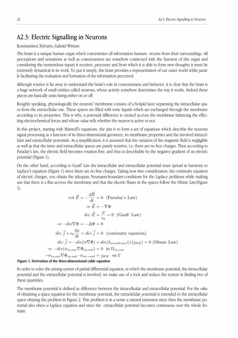
In this project, starting with Maxwell's equations, the aim is to form a set of equations which describe the neuronssignal processing as a function of its three-dimensional geometry, its membrane properties and the involved intracel-lular and extracellular potentials. As a simplification, it is assumed that the variation of the magnetic field is negligibleas well as that the intra- and extracellular spaces are purely resistive, i.e. there are no free charges. Then according toFaraday's law, the electric field becomes rotation free, and thus is describable by the negative gradient of an electricpotential (Figure 1).

On the other hand, according to Gauß' Law the intracellular and extracellular potential must spread in harmony toLaplace's equation (Figure 1) since there are no free charges. Taking now into consideration, the continuity equationof electric charges, you obtain the adequate Neumann-boundary-conditions for the Laplace problems while makinguse that there is a flux accross the membrane and that the electric fluxes in the spaces follow the Ohmic Law(Figure1).

22 A2.3: Electric Signalling in Neurons

Figure 1. Derivation of the three-dimensional cable equation

In order to solve the arising system of partial differential equation, in which the membrane potential, the intracellularpotential and the extracellular potential is involved, we make use of a trick and reduce the system in finding two ofthese quantities.

The membrane potential is defined as difference between the intracellualar and extracellular potential. For the sakeof obtaining a space equation for the membrane potential, the extraclelular potential is extended to the intracellularspace obaying the problem in Figure 2. This problem is in a sense a natural extension since then the membrane po-tential also obeys a Laplace equation and since the extracellular potential becomes continuous over the whole do-main.

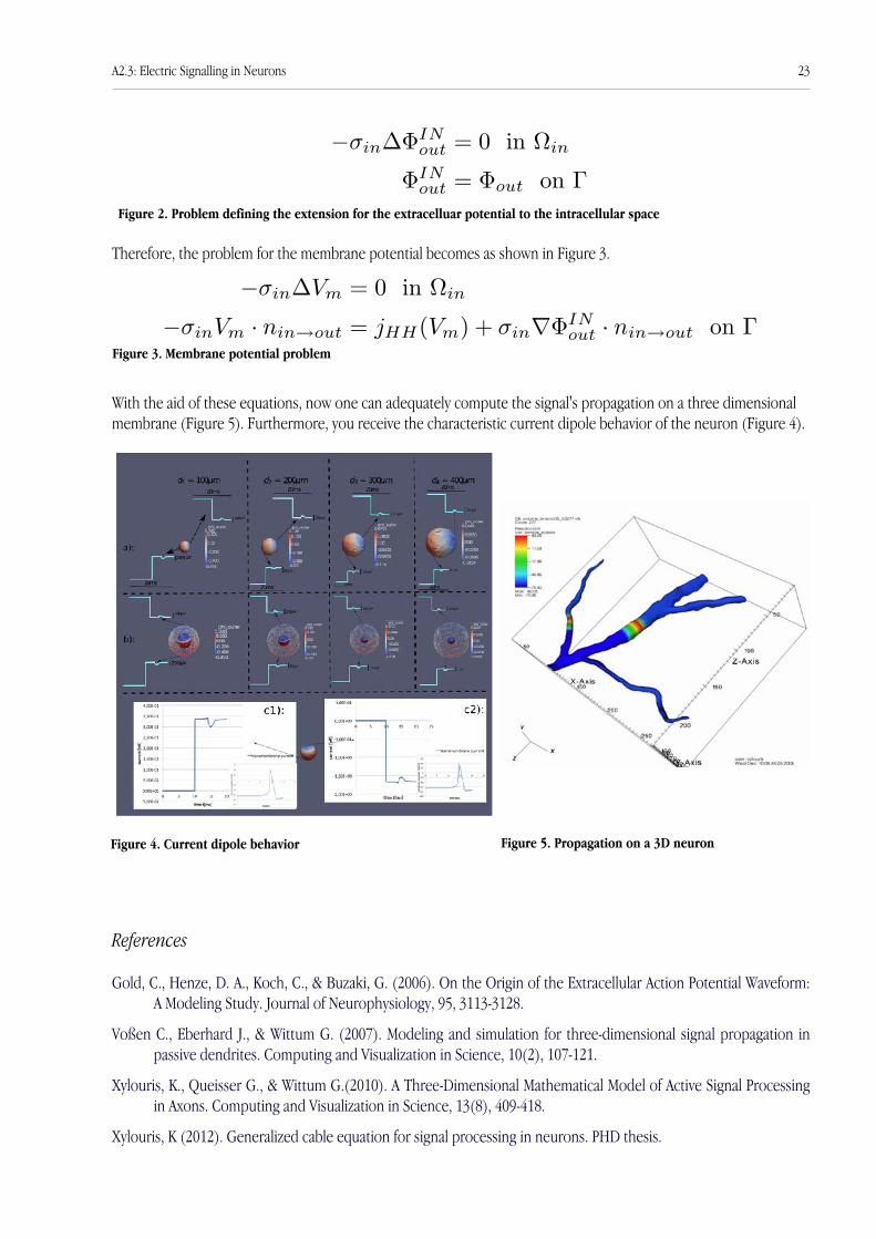
Therefore, the problem for the membrane potential becomes as shown in Figure 3.

With the aid of these equations, now one can adequately compute the signal's propagation on a three dimensionalmembrane (Figure 5). Furthermore, you receive the characteristic current dipole behavior of the neuron (Figure 4).

References

Gold, C., Henze, D. A., Koch, C., & Buzaki, G. (2006). On the Origin of the Extracellular Action Potential Waveform:A Modeling Study. Journal of Neurophysiology, 95, 3113-3128.

Voßen C., Eberhard J., & Wittum G. (2007). Modeling and simulation for three-dimensional signal propagation inpassive dendrites. Computing and Visualization in Science, 10(2), 107-121.

Xylouris, K., Queisser G., & Wittum G.(2010). A Three-Dimensional Mathematical Model of Active Signal Processingin Axons. Computing and Visualization in Science, 13(8), 409-418.

Xylouris, K (2012). Generalized cable equation for signal processing in neurons. PHD thesis.

A2.3: Electric Signalling in Neurons 23

Figure 4. Current dipole behavior

Figure 2. Problem defining the extension for the extracelluar potential to the intracellular space

Figure 3. Membrane potential problem

Figure 5. Propagation on a 3D neuron

A2.4: Modelling Replication Dynamics of Hepatitis C Virus in 3D SpaceMarkus Knodel, Alfio Grillo, Paul Targett-Adams, Eva Herrmann, Gabriel Wittum

Hepatitis C virus is the major cause of nowadays liver diseases in western countries. The Heptatitis C virus (HCV) in-fection is caused by blood-to-blood contacts to infected persons. HCV causes in nearly all cases a chronic liver infec-tion. Within several years, many patients develop liver chirrhosis and even liver cancer. Therefore, many of themneed liver transplantation or die, in each case their life quality is reduced strongly. There exist several genotypes ofHCV, for some of them medical treatments could be developed (combined Interferon and Ribivarin therapy) whichhelp a significant part of the patients, however for several genotypes there is no treatment available up to now. Inparticular, there is no vaccinatiojn available and this could hold on for many years still. Recently, there was progresswith respect to the development of new antiviral drugs which block viral processing in parts, but nevertheless thereis only few progress in understanding the complete replication dynamics and the experimental possibilities are ratherrestricted due to the lack of small animal model systems, i.e. the virus only replicates in high developed primates andonly up to some extend in cell cultures. Even though there exist some mathematical models which allowed for un-derstanding of some basic relations, no one of these take into account the spatial structure of the liver cells in whichthe virus gets replicated. Therefore, our aim is to apply our instrument of in silico 3D simulation techniques to thisfield in order to allow for new insights with respect to viral replication fror the sake of modeling in detail the effectsof new antiviral agents allowing for more effective strategies with respect to the development of new antiviral agents.

HCV is an enveloped, positive stranded RNA virus and belongs to the family of Flaviviridiae, to which also belong e.g.yellow and Dengue fever. Once it fuses with the membrane of a hepatocyte (liver cell), it gets endocytosed. Insidethe cytosol, the RNA gets uncoated and gets translocated to the rough Endoplasmatic Reticulum (rough ER / rER).

There, it fuses with ribosomes and this causes the translati-on of a big number of the viral polyprotein. The polyproteingets cleaved in parts by cellular proteases and in other partsby viral proteases. There are as well structural and nonstruc-tural proteins. At first, the structrural proteins are cleavedby cellular proteases. The structural proteins will later en-close the new viral RNA (which will be produced in forthco-ming steps by replication of the existing one). In particular,the core protein C will have to enclose the RNA and the en-velope proteins E1 and E2 will bind to the surface in orderto enable the entry to other cells once the new viral particlewill have been freed by the actual cell. However beforebeing able to do so, first the nonstructural proteins have tocause the reproduction of the existing RNA. This gets donein the following way: After when the structural proteins are

cleaved by cellular proteases from the polyprotein (and a small protein called p7 of which the function is not clear sofar'), the rest of the polyprotein cleaves independently of cellular processes. In particular, at first the nonstructuralprotein NS2 cleaves autocatalytically. Then the combination of the NS3 and NS4a (NS3/4a protease) frees the RNApolymerase NS5b, the multifunctional NS5a (which is especially related to the suppression of the cellular immune re-sponse) and the NS4b. Finally also NS3 and NS4a are seperated. The NS4b protein causes on top of the membrane ofthe ER the growing of regions of the so-called membranous web, which is the accumulation of many small vesicles.Soon there exist several regions on the surface of the ER where this vesicular places are located, the bigger of theseregions are more or less spatially fixed whereas the smaller ones are "jumping" around presumably randomly. Oncethese web regions exist, the RNA polymerase NS5b proteins get translocated into them. For not understood reasons,at some step the so far only existing (old) viral RNA translocates into one of these web regions causing its own repro-duction by the NS5b polymerase. At intermediate steps, negative stranded RNA gets produced and combines withthe plus-stranded one to double stranded RNA (dsRNA) allowing for producing new plus-stranded RNA. In parts thenew RNA will translocate again to ribosomes causing the production of new polyproteins, others will go to other web

24 A2.4: Modelling Replication Dynamics of Hepatitis C Virus in 3D Space

Figure 1. The Hepatitis C life cycle: Uncoating and transla-tion of the RNA, cleavage of the polyprotein, creation ofthe membranous web, reproduction of the RNA and as-sembly and exocytosis of new viruses

regions causing production of additional RNAs. Thus the circle of RNA reproduction gets cloesd. At some step, coreproteins accumulates at the surfaces of so-called lipid droplets, forming hulls, and into this hull, RNA will get incor-

porated. The E1 and E2 proteins will fuse with the surface, and in some notunderstood way new complete viruses will leave the cell on the usual secre-tory pathway within vesicles passing inparticular also the Golgi apperatus. Themature viruses will get exocytosed final-ly at the surface of the cell. The aim ofantiviral agants is to block one or se-veral of the reproduction steps.

We are creating a biophysical model ofthe replication of the virus within thecomplete spatio-temporal domain of sin-gle hepatocytes. Therefore we are re-constructing the geometry of the ER of

hepatocyte confocal flouroscence microscopy image z-stack data (using NeuRA2) corresponding to calnexin markerwhich localizes on the surface of the ER. On top of this geometry we will do simulations of the dynamics of the viralproteins and RNA (using UG) allowing for precise predictions with respect to the effects of antiviral agents hence al-lowing for more effective pharmaceutical development.

ReferencesDahari, H., Ribeiro, R. M., Rice, C. M., & Perelson, A. S. (2007). Mathematical Modeling of Subgenomic Hepatitis C Virus Repli-

cation in Huh-7 Cells. Journal of Virology, 81(2), 750-760.

Kwong, A. D., Kauffman, R. S., Hurter, P., & Mueller, P. (2011). Discovery and development of telaprevir: an NS3-4A proteaseinhibitor for treating genotype 1 chronic hepatitis C virus. Nature Biotechnology, 29, 993–1003.

Moradpour, D., Penin, F., & Rice, C. M. (2007). Replication of hepatitis C virus. Nature Reviews Microbiology, 5, 453–463.

Targett-Adams, P., Boulant, S., & McLauchlan, J. (2008). Visualization of Double-Stranded RNA in Cells Supporting Hepatitis CVirus RNA Replication. Journal of Virology, 82(5), 2182-2195.

Targett-Adams, P., Graham, E. J. S., Middleton, J., Palmer, A., Shaw, S. M., Lavender, H., Brain, P., Tran, T. D., Jones, L. H., Wa-kenhut, F., Stammen, B., Pryde, D., Pickford, C., & Westby, M. (2011). Small Molecules Targeting Hepatitis C Virus-En-coded NS5A Cause Subcellular Redistribution of Their Target: Insights into Compound Modes of Action. Journal of Vi-rology, 85(13), 6353-6368.

Wölk, B., Büchele, B., Moradpour, D., & Rice, C. M. (2008). A Dynamic View of Hepatitis C Virus Replication Complexes. Jour-nal of Virology, 82(21), 10519-10531.

A2.4: Modelling Replication Dynamics of Hepatitis C Virus in 3D Space 25

Figure 2. Regions of replication ("mem-branous web") at the ER

Figure 3. Confocal flouroscencemicroscopy image of calnexin, anER marker

Figure 4a and b. 3D reconstructions of the ER (marked by calnexin), thedouble stranded viral RNA and the lipid droplets (marked by ADRP). Actu-ally redone using NeuRA

A2.5: NeuClass: Neuron Classification ToolsHolger Heumann, Gabriel Wittum

In the age of technological leaps in the neuroscientific world, a multitude of research areas, computational tools,mathematical models and data-aquiring methods have emerged and are rapidly increasing. Not only is data massexploding, but also different data types and research approaches account for large diversification of data and tools. Atthe G-CSC ongoing research of an interdisciplinary nature brought about the need for organised and automatic data& tool structuring. Furthermore, we see a central data & tools management as an optimal means for scientificknowledge exchange, especially in decentralised research projects.

In addition to the automatic reconstruction of neuron morphologies by NeuRA, a new tool has been developed forthe automatic classification of cells, NeuClass. This is a typical entry point of data into the database. Thus wedeveloped a new approach for the classification of neuron cells.

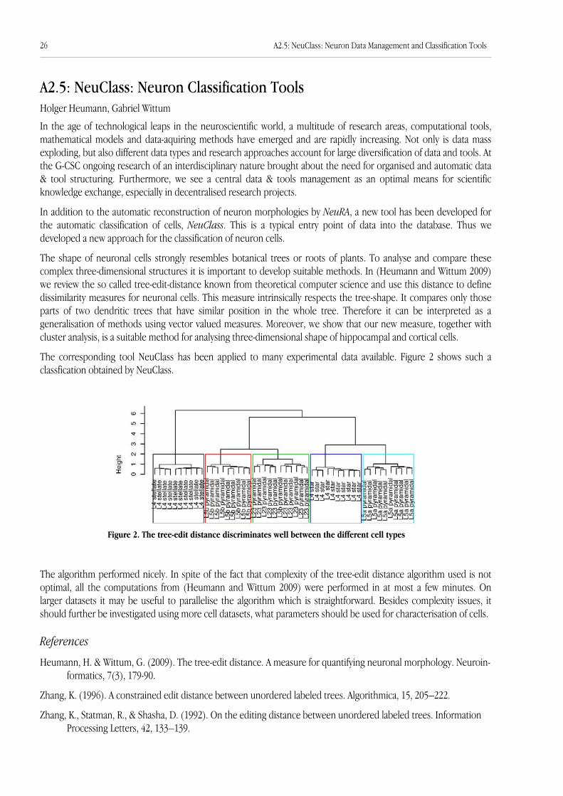
The shape of neuronal cells strongly resembles botanical trees or roots of plants. To analyse and compare thesecomplex three-dimensional structures it is important to develop suitable methods. In (Heumann and Wittum 2009)we review the so called tree-edit-distance known from theoretical computer science and use this distance to definedissimilarity measures for neuronal cells. This measure intrinsically respects the tree-shape. It compares only thoseparts of two dendritic trees that have similar position in the whole tree. Therefore it can be interpreted as ageneralisation of methods using vector valued measures. Moreover, we show that our new measure, together withcluster analysis, is a suitable method for analysing three-dimensional shape of hippocampal and cortical cells.

The corresponding tool NeuClass has been applied to many experimental data available. Figure 2 shows such aclassfication obtained by NeuClass.

The algorithm performed nicely. In spite of the fact that complexity of the tree-edit distance algorithm used is notoptimal, all the computations from (Heumann and Wittum 2009) were performed in at most a few minutes. Onlarger datasets it may be useful to parallelise the algorithm which is straightforward. Besides complexity issues, itshould further be investigated using more cell datasets, what parameters should be used for characterisation of cells.

References

Heumann, H. & Wittum, G. (2009). The tree-edit distance. A measure for quantifying neuronal morphology. Neuroin-formatics, 7(3), 179-90.

Zhang, K. (1996). A constrained edit distance between unordered labeled trees. Algorithmica, 15, 205–222.

Zhang, K., Statman, R., & Shasha, D. (1992). On the editing distance between unordered labeled trees. InformationProcessing Letters, 42, 133–139.

Figure 2. The tree-edit distance discriminates well between the different cell types

26 A2.5: NeuClass: Neuron Data Management and Classification Tools

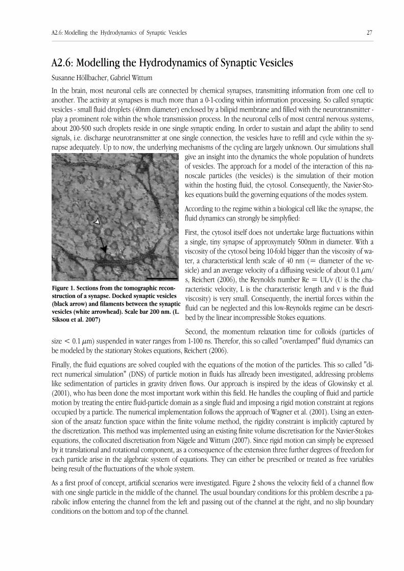
A2.6: Modelling the Hydrodynamics of Synaptic Vesicles Susanne Höllbacher, Gabriel Wittum

In the brain, most neuronal cells are connected by chemical synapses, transmitting information from one cell toanother. The activity at synapses is much more than a 0-1-coding within information processing. So called synapticvesicles - small fluid droplets (40nm diameter) enclosed by a bilipid membrane and filled with the neurotransmitter -play a prominent role within the whole transmission process. In the neuronal cells of most central nervous systems,about 200-500 such droplets reside in one single synaptic ending. In order to sustain and adapt the ability to sendsignals, i.e. discharge neurotransmitter at one single connection, the vesicles have to refill and cycle within the sy-napse adequately. Up to now, the underlying mechanisms of the cycling are largely unknown. Our simulations shall

give an insight into the dynamics the whole population of hundretsof vesicles. The approach for a model of the interaction of this na-noscale particles (the vesicles) is the simulation of their motionwithin the hosting fluid, the cytosol. Consequently, the Navier-Sto-kes equations build the governing equations of the modes system.

According to the regime within a biological cell like the synapse, thefluid dynamics can strongly be simplyfied:

First, the cytosol itself does not undertake large fluctuations withina single, tiny synapse of approxymately 500nm in diameter. With aviscosity of the cytosol being 10-fold bigger than the viscosity of wa-ter, a characteristical lenth scale of 40 nm (= diameter of the ve-sicle) and an average velocity of a diffusing vesicle of about 0.1 µm/s, Reichert (2006), the Reynolds number Re = UL/v (U is the cha-racteristic velocity, L is the characteristic length and v is the fluidviscosity) is very small. Consequently, the inertial forces within thefluid can be neglected and this low-Reynolds regime can be descri-bed by the linear incompressible Stokes equations.

Second, the momentum relaxation time for colloids (particles ofsize < 0.1 µm) suspended in water ranges from 1-100 ns. Therefor, this so called "overdamped" fluid dynamics canbe modeled by the stationary Stokes equations, Reichert (2006).

Finally, the fluid equations are solved coupled with the equations of the motion of the particles. This so called "di-rect numerical simulation" (DNS) of particle motion in fluids has allready been investigated, addressing problemslike sedimentation of particles in gravity driven flows. Our approach is inspired by the ideas of Glowinsky et al.(2001), who has been done the most important work within this field. He handles the coupling of fluid and particlemotion by treating the entire fluid-particle domain as a single fluid and imposing a rigid motion constraint at regionsoccupied by a particle. The numerical implementation follows the approach of Wagner et al. (2001). Using an exten-sion of the ansatz function space within the finite volume method, the rigidity constraint is implicitly captured bythe discretization. This method was implemented using an existing finite volume discretisation for the Navier-Stokesequations, the collocated discretisation from Nägele and Wittum (2007). Since rigid motion can simply be expressedby it translational and rotational component, as a consequence of the extension three further degrees of freedom foreach particle arise in the algebraic system of equations. They can either be prescribed or treated as free variablesbeing result of the fluctuations of the whole system.

As a first proof of concept, artificial scenarios were investigated. Figure 2 shows the velocity field of a channel flowwith one single particle in the middle of the channel. The usual boundary conditions for this problem describe a pa-rabolic inflow entering the channel from the left and passing out of the channel at the right, and no slip boundaryconditions on the bottom and top of the channel.

A2.6: Modelling the Hydrodynamics of Synaptic Vesicles 27

Figure 1. Sections from the tomographic recon-struction of a synapse. Docked synaptic vesicles(black arrow) and filaments between the synapticvesicles (white arrowhead). Scale bar 200 nm. (L.Siksou et al. 2007)

Varying now the horizontal location of the particle within ofthe channel, the velocity of the inserted particle - passivelydriven by the sourrounding flow field - changes. This depen-dence is ploted in Figure 3. As to be expected, the particlebeing located in the lower or upper half of the channel ap-proaches the center (blue triangles, contour). With decrea-sing distance from the center its velocity in x-direction in-creases (blue triangles, filled). The rotational velocity chan-ges orientation passing the zero-line of the y-axis (red squa-res).

In order to apply these technique to the simultaion of synaptic vesicles, certain features has to be added, like the ge-ometrical information of the location of certain vesicles, the morphological properties of the synapse and the biologi-cal forces dominating this regime. This will be part of the ongoing work.

References

Glowinski, R., Pan, T.W., Hesla, T.I., Joseph, D.D., & Périaux, J. (2001). A Fictitious Domain Approach to the DirectNumerical Simulation of Incompressible Viscous Flow past Moving Rigid Bodies: Application to ParticulateFlow. Journal of Computational Physics, 169(2), 363-426.

Nägele, S., & Wittum, G. (2007). On the influence of different stabilisation methods for the incompressible Navier-Stokes equations. Journal of Computational Physics, 224(1), 100-116.

Reichert, M. (2006). Hydrodynamic Interactions in Colloidal and Biological Systems. Dissertation, URL: http://ub.uni-konstanz.de/kops/volltexte/2006/1930/.

Wagner, G. J., Moes, N., Liu, W. K., & Belytschko, T. (2001). The extended finite element method for rigid particles inStokes Flow. International Journal for Numerical Methods in Engineering, 51, 293–313.

28 A2.6: Modelling the hydrodynamics of synaptic vesicles

Figure 2. Velocity field of the channel problem with one inserted particle in the middle of the channel

Figure 3. Plot of the free velocities of an inserted particle

A3.1, CF3: The Numerical Pricing of Options with Many Risk FactorsPhilipp Schröder, Christoph Reisinger, Gabriel Wittum

A very large and increasing number of products traded on financial markets has the form of derivative securities. It iscommon that these products depend on several uncertain quantities that have to be modelled as stochastic parame-ters. Two particular examples in this wide range of products are FX options on the exchange rate between two cur-rencies, where the dynamics of the interest rates on the two markets is also crucial, or basket options, which dependon the average of a possibly very large selection of stocks. It is common to express the risky assets and stochastic pa-rameters in terms of Brownian motions, giving rise to parabolic PDEs for the option price. The need for efficienttechniques to price these contracts faster and more reliably than by means of state-of-the-art Monte Carlo methodsis enormous.

The focus of our research is multivariate systems such as those mentioned above with a special emphasis on high-di-mensional problems. First, taking into account the correlation of the processes, a reduced model with a low super-position dimension is derived. This allows a very accurate extrapolation of the solution from lower-dimensionalproblems. The resulting parabolic equations are discretised on sparse grids with a drastically reduced number ofpoints compared to the conventional spaces. The combination technique allows a further decoupling into discretesubspaces. These linear systems are solved by a suitable multilevel solver in linear complexity . The robust solution isessential for the speed-up of the parallel implementation of the method.

Dimensional reduction

High-dimensional processes often show a typical correlation pattern corresponding to a characteristic form of thespectrum: a dominating component represents the movement of the market, the other eigenvalues decay exponen-tially. Asymptotic analysis can be used to study the perturbations of simple one-factor models. For the classicalBlack-Scholes model, an analytic expansion of the solution in terms of these small parameters has been derived. Asan alternative, the solution is extrapolated from two-dimensional auxiliary problems that mimic the directional deri-vatives with respect to the spectrum. The latter idea can be carried over to more general situations. Recently, a theo-retical background to explan the good practical results of the asymptotic expansion has been devoloped (Schröder2012).

Sparse grids and multigrid methodsSparse grids are known to break the “curse of dimensionality”, i.e. the exponentially increasing number of gridpoints in high dimensions. The combination technique exploits an astonishing extrapolation property of a particularfamily of hierarchical subspaces: Assuming some form of the error expansion for the discretisation scheme, the com-

A3.1: Option Pricing 29

Figure 1. Complexity reduction for option pricing problem

bination of solutions on decoupled Cartesian grids shows the same asymptotic error as the sparse finite element so-lution and deteriorates only by logarithmic factors in comparison with the full high-dimensional Cartesian grid. In thecourse of this project, the above statement could be proven and closed form error estimates for the sparse-grid solu-tion in arbitrary dimensions have been derived.

The parallel implementation gave very accurate results for real-world scenarios in up to six dimensions. A solver of li-near complexity is crucial for the load balancing. A multilevel technique with “plane” smoothing, applied recursivelyin lower-dimensional hyper-planes, proved robust for the present anisotropic and degenerate parabolic operators co-ming from bounded stochastic processes. Extensions to American options involve adapted transfer operators at thefree boundary and show comparable convergence.

Results

The plot shows the price u of a European option on a basket of two uncorrelated stocks S1 and S2 with different vola-tilities. The triangle indicates the pay-off, which serves as terminal condition. The sparse grid has been transformedsuch that the kink in the pay-off is captured exactly and graded in the direction orthogonal to the kink. This preser-ves the discretisation order despite the lack of smoothness and provides a suitable refinement in that region.

For visualisation‘s sake, we show only two-dimensional results in the figure above. Nevertheless, comparison with so-lutions obtained by a large number of Monte Carlo runs shows that our approach yields remarkably accurate priceswithin a few minutes with errors below 0.1 % even for very large baskets like the DAX (30 dimensions).

References

Reisinger, C. (2004). Numerische Methoden für hochdimensionale parabolische Gleichungen am Beispiel vonOptionspreisaufgaben (Numerical Methods for High-Dimensional Parabolic Equations on the Example ofOption Pricing Problems). PhD thesis, University of Heidelberg.

Reisinger, C., & Wittum, G. (2004). Multigrid Methods for Anisotropic Equations and Variational Inequalities. Com-puting and Visualisation in Science, 7(3-4), 189-197.

Reisinger, C., & Wittum, G. (2007). Efficient Hierarchical Approximation of High-Dimensional Option Pricing Prob-lems. SIAM Journal on Scientific Computing, 29(1), 440-458.

Schröder, P., Gerstner, T., & Wittum, G. (2012). Taylor-like ANOVA Expansion for high dimensional Problems in Fi-nance. Manuscript submitted for publication.

30 A3.1: Option Pricing

Figure 2. Result and payoff function (black) oftwo-asset basket option

A3.2, CF4: Credit Risk Estimation in High DimensionsPhilipp Schröder, Gabriel Wittum

Credit risk influences many important banking processes and functions like credit decisions and pricing, portfoliomanagement, estimation of portfolio losses, building of loan loss reserves, etc. Thus, the correct quantification ofcredit risk is crucial for a bank. The credit risk basically consists of four components: loan exposure, (payment) de-fault probability of the borrower (PD), potential recovery after default due to collateral, and (default) correlation ofthe borrowers.

The modelling of customers default correlations is an important research area. Borrower correlations are currentlyonly considered in sophisticated credit portfolio models. Nevertheless, these correlations are as well important. forthe calculation of default probabilities of complex exposure structures (for instance loans to a group of linked com-panies) or for the calculation of the joint default probability of borrower and guarantor. Recently, modern numericalanalysis techniques have been successfully applied to option pricing problems (Reisinger 2004). As option pricingand Merton-type credit portfolio models are based on the same rationale, the objective of our recent research was tocombine the classical Merton-type portfolio model (Merton 1974) with advanced numerical methodologies like spar-se grids and multigrid solvers in order to obtain an efficient borrower correlation model.

Since the resulting partial differential equations are of high dimensionality, different approaches have been taken toincrease efficiency of the used algorithms.

Dimensional reduction

As many problems from finance, the estimation of joint default probabilities for large portfolios suffers from the socalled „curse of dimension“ due to the high number of underlying risk drivers. Statistical analysis (e.g. Analysis of Va-riance, Principal Component Analysis) of the underlying processes however often shows, that the original problemcan be decomposed into problems of lower dimension. Furthermore only some of the lower dimensional subprob-lems have significant contribution to the total variance of the problem. The picture below shows an ANOVA analysisof two-dimensional subproblems a 30D highly correlated credit portfolio can be decomposed in. Subproblems thatcontribute to the total variance of the problem significantly are shown in brown.

Asymptotic expansion can be used to extrapolate the solution of the fully dimensional problem via a linear combina-tion of the individual solutions to the subproblems. For the classical Merton Firm Value model, an expansion of thesolution in terms of these subproblems has been derived (Schröder 2009).

A3.2: Credit Risk Estimation 31

Figure 1. ANOVA Analysis of two-dimensional sub-problems

Recently, a higher order expansion has been developed. Additionally, a theoretical background for the good practicalresults has been developed (Schröder 2011, Schröder 2012)

Parallelization

The parallel implementation of a sparse grid extrapolation technique gave very accurate results together with goodscalability results for real-world scenarios up to six dimensions. Current research is aimed on the developement ofan additional layer for the parallelization, i.e. a parallelization of the calulation of the subproblems solutions.

Results

Asymptotic expansion and sparse grid combination technique enabled us to efficiently calculate the default risk for aportfolio of 50 higly correlated credits with relative errors below 0.1%.

References

Merton, R. C. (1974). On the pricing of corporate debt: The risk structure of interest rates. The Journal of Finance,29(2), 449-470.

Mlynczak, P. (2011). Parallelization concepts for the solution of high-dimensional PDEs with applications in finance.Master thesis, Universität Frankfurt.

Reisinger, C. (2004). Numerische Methoden für hochdimensionale parabolische Gleichungen am Beispiel von Opti-onspreisaufgaben (Numerical Methods for High-Dimensional Parabolic Equations on the Example of OptionPricing Problems). PhD thesis, Universität Heidelberg.

Schröder, P., Avçu, Y., Wagner, C. & Wittum, G. (2009). Calculation of Default Probability (PD) solving Merton ModelPDEs on Sparse Grids. Proceedings of the 23rd IPDPS, IEEE International Symposium on Parallel&DistributedProcessing, pp.1-6.

Schröder, P. (2011). Dimensionsweise Zerlegungen hochdimensionaler Probleme mit Anwendungen im Finanzbe-reich, PhD thesis, Universität Frankfurt, submitted.

Schröder, P., Gerstner, T., & Wittum, G. (2012). Taylor-like ANOVA Expansion for high dimensional Problems in Fi-nance, Manuscript submitted for publication

32 A3.2: Credit Risk Estimation

Figure 2. Scaleup for six-dimensional problem Figure 3. Absolute Error for six-dimensional problem

A3.3, CF5: Portfolio OptimisationMathias Höfer, Holger Kraft, Gabriel Wittum

An important problem in modern continuous time finance is the so-called Merton's Lifetime Portfolio Problem. Whe-reas the former portfolio selection approach by Markowitz regards an isolated portfolio without dynamic effects, thistime-dependent model becomes more realistic (Merton 1969). Succeeding authors constructed generalised models,which made it difficult or even impossible to find closed-form solutions. Numerical methods can handle these kindof higher dimensional problems.

The task is finding an optimal strategy for the level of consumption and investment in different risky assets to reachmaximum expected utility. The regarded model consists of two important parts. First, an economy, which is model-led by the interest rate and diverse market prices e.g. of shares or bonds. The dynamics of these market characteris-tics are expressed in terms of correlated stochastic processes based on the Brownian Motion. Secondly, the consu-mer/small investor is modelled by his utility function, which shows his risk aversion and his consumption require-ments, furthermore his income is modelled stochastically similar to the market processes. The optimal value func-tion (maximum expected utility) is composed of the discounted utility of running consumption and the discountedfinal wealth. This problem of stochastic control theory can be transformed to a controlled partial differential equati-on, the so-called Hamilton-Jacobi-Bellman Equation. Ignoring the maximization problem, this equation is a convec-tion-diffusion equation with source terms, whereby the choice of the investment strategy has linear effects on thedrift-terms and quadratic influence on the diffusion. Changes of consumption level itself causes non-linearamendments.

Classical solvers require finite control possibilies in each discretized time step (Lion and Mercier 1980). The princi-ple work flow of the solver is an alternating process of finding the maximizing strategy parameters and computingthe partial differential equation. Integrating a gradient descent optimizer enables continous investment and con-sumption choise. The capabilies of SG2 can be used to construct a fast HJB-solver with the described method.The concept of sparse grids allows decreasing the number of grid points substantially (Reisinger and Wittum 2007).Constructing a hierarchy of coarser grids gives the opportunity to identify relevant strategy-combinations and consi-der them on finer levels as initialisation for the optimiser. This adapted nested iteration method offers the opportu-nity to reduce calculation time. Combining the solution of HJB-equation and the corresponding strategy-vectorswith typical sparse-grid-methods leads to demanded solution.

Illustrating a 3-dimensional problem, one can see the optimal strategy of an exemplary consumer in diverse marketenvironments.

A3.3: Portfolio Optimisation 33

Figure 1. Optimal investment strategy and consumption of a smallinvestor.

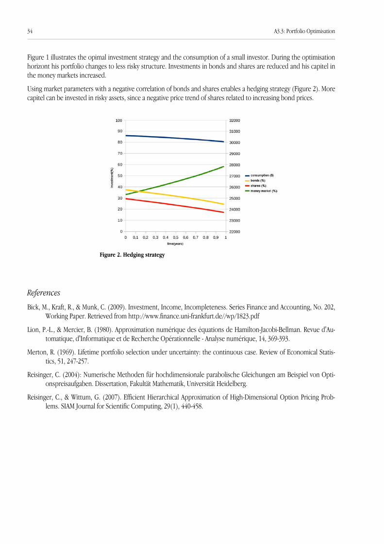
Figure 1 illustrates the opimal investment strategy and the consumption of a small investor. During the optimisationhorizont his portfolio changes to less risky structure. Investments in bonds and shares are reduced and his capitel inthe money markets increased.

Using market parameters with a negative correlation of bonds and shares enables a hedging strategy (Figure 2). Morecapitel can be invested in risky assets, since a negative price trend of shares related to increasing bond prices.

References

Bick, M., Kraft, R., & Munk, C. (2009). Investment, Income, Incompleteness. Series Finance and Accounting, No. 202,Working Paper. Retrieved from http://www.finance.uni-frankfurt.de//wp/1823.pdf

Lion, P.-L., & Mercier, B. (1980). Approximation numérique des équations de Hamilton-Jacobi-Bellman. Revue d'Au-tomatique, d'Informatique et de Recherche Opérationnelle - Analyse numérique, 14, 369-393.

Merton, R. (1969). Lifetime portfolio selection under uncertainty: the continuous case. Review of Economical Statis-tics, 51, 247-257.

Reisinger, C. (2004): Numerische Methoden für hochdimensionale parabolische Gleichungen am Beispiel von Opti-onspreisaufgaben. Dissertation, Fakultät Mathematik, Universität Heidelberg.

Reisinger, C., & Wittum, G. (2007). Efficient Hierarchical Approximation of High-Dimensional Option Pricing Prob-lems. SIAM Journal for Scientific Computing, 29(1), 440-458.

Figure 2. Hedging strategy

34 A3.3: Portfolio Optimisation

A4.1: Simulation of Crystal Growth and Attrition in a Stirred TankDmitry Logashenko, Torsten Fischer, Gabriel Wittum

Crystallisation from solution in stirred crystallisers is one of the economically most important industrial separationand purification processes. It is applied as a large scale continuous process for the production of inorganic (e.g. po-tassium chloride, ammonium sulphate) and organic (e.g. adipic acid) materials. On a small scale it is often applied asa batch operation to produce high purity pharmaceuticals or fine chemicals (e.g. aspartame, L-ascorbine). This pro-cess includes two classes of physically different but strongly coupled phenomena. The first one is the crystallisationitself, typically described by means of population models. The second one consists of the spatial flow and the trans-port induced by the stir.

We consider a continuous stirred crystalliser (cf. Figure 1). The pure solution (without crystals) is pumped in at theinflow and the suspension of the crystals leaves the tank at the outflow so that the volume of the fluid in the tank isconstant. The crystalliser is cooled from the outside so that the solution in it is oversaturated. The attrition of thecrystals happence only on the stirrer whereas the growth takes place everywhere in the tank. The fluid in thecrystalliser is suspension whose density and viscosity depend on the concentration of the crystals and the dissolvedsubstance.

The main feature of this model is its hight dimensionality: 2 or 3 spatial dimentions for the flow and the transportare extended with one additional dimention for the population dynamics. (We assume that the crystals have onlyone inner parameter - the length.) A practically relevant description of complicated behaviour of the crystallisationprocess requires a fine numerical resolution in this crystall length dimension. Furthermore, the population balanceequations include integral terms that need special numerical treatment. This leads to a high computational comple-xity of the simulations that can be only achieved under the use of parallel architectures and adaptive techniques.

The geometric space is covered with an unstructured grid. On it, the coupled flow and transport equations arediscretised to one nonlinear algebraic system (we use the implicit time scheme) that can be then solved by the fixed-point or Newton iteration. The arising linear systems are handled by the geometrical multigrid method with the ILU-smoothers. The unstructured grid is adaptively refined during the time stepping according to an error indicator. Atevery node of this grid, we introduce a uniform mesh for the discretisation of the population balance equations.

Figure 2 presents the results of the simulation of crystallisation of potassium nitrate in a stirred tank (cf. Logashenkoet al. 2006). The inflow is placed at the upper part of the left wall and the outflow at the lower part of the right one(s. the upper left picture in this figure). The stirrer is located in the middle of the crystalliser. The pictures corre-spond to time 300 s from the beginning of the process, when the tank was filled with the suspension of the middle-sized crystals. The spatial unstructured grid consists of about 12500 nodes, the population mesh has 51 points (atevery node of the spatial grid). This simulation shows the fine spatial structuring of the process.

Similar results of the simulation in a 3d crystalliser are illustrated in Figure 3. The pictures have here the same mea-ning as on Figure 2 and represent an early stage (1.5 s) of the process.

A4.1: Simulation of Crystal Growth and Attrition in a Stirred Tank 35

Figure 1. Scheme of the stirred crystalliser

References

Fischer, T., Kirkilionis, M., Logashenko, D. & Wittum, G. (2006): Fast Numerical Integration for Simulation ofDisperse Systems. Mathematical Models and Methods in Applied Sciences, 16(12), 1987-2012.

Logashenko, D., Fischer, T., Motz, S., Gilles, E.-D., & Wittum, G. (2006). Simulation of Crystal Growth and Attrition ina Stirred Tank. Computing and Visualization in Science, 9(3), 175-183.

Figure 3. Crystallisation of potassium nitrate in a stirred tank (3d simulation)The meaning of the plots is the same as for Figure 2.

Figure 2. Crystallisation of potassium nitrate in a stirred tank (2d simulation)Upper pictures (f.l.t.r.): the flow velocity field [m/s], the molar fraction of the substance in the solution and the temperature [oC]. Lowerpictures: the integral volume fraction for lengths 0-0.1 mm, 0.1-0.5 mm and 0.5-1 mm.

36 A4.1: Simulation of Crystal Growth and Attrition in a Stirred Tank

A5.1: Density-Driven Flow in Porous Media 37

A5: Environmental ScienceA5.1: Density-Driven Flow in Porous MediaAlfio Grillo, Michael Lampe, Gabriel Wittum

A leading topic in hydrogeology and environmental science is the investigation of salinity- and thermohaline-drivenfluid flow in porous media of hydrological relevance. The porous medium and the fluid are usually identified with asoil and groundwater, respectively. The name given to these two types of groundwater flow depends on the causesthat have either brought the fluid out of mechanic equilibrium or altered its dynamic state. Salinity-driven flow isdue to the non-uniform change of the mass density of the fluid consequent to mixing together water and brine (thelatter is a mixture of water and various salts). Temperature-driven flow is triggered by exposing the fluid to thermalgradients or mixing together flows at different temperatures. Thermohaline-driven flow is the combined effect of thejust mentioned types of flows. In all these cases, in order to observe flow, it is necessary that the alteration of thedensity of the fluid favours fluid motion. Within the context sketched above, some of the most typically studiedproblems are sea-water intrusion into coastal aquifers, upconing of hypersaline water from deep aquifers, flowaround salt domes or sedimentary rocks, and contamination of aquifers caused by waste. Some of the reasons forundertaking these studies are the managment of freshwater supplies (especially in arid or urbanised zones) and thesolution forcast and remediation problems (for example, in the neighbourhood of nuclear waste repositories).

Our research focussed on the mathematical modelling, numerical simulation, and physical interpretation of somepeculiar phenomena of thermohaline-driven flow that can be captured through the analysis of dedicated benchmarkproblems. The theoretical aspects of our investigations are inspired by Hassanizadeh (1986) and Bear (1972). Nume-rical simulations were carried out by using the sofware packages ⋲ and d3f (Fein 1998). A summary of our results,which also covered the study of thermodiffusion in porous media, was provided by Grillo et al. (2011). More detai-led, three-dimensional simulations of thermohaline-driven flow as well as brine and heat transport were done in thepublications by Grillo et al. (2010) and Lampe et al. (2010), where the buoyancy of a brine parcel was studied. The si-mulations consist of a generalisation of the benchmark proposed by Oldenburg and Pruess (1999). Some of our re-sults are shown in the following figures. Recently, we extended our results to the case of fractured porous media(Grillo et al. 2012, Stichel et al. 2012).

Some results of the simulations concerning the buoyancy of a brine parcel are reported in the figures. The peculiarphenomenological features of this example can be summarised as follows. In the case of negative buoyancy, brine istransported downward faster than heat because of a retardation factor, which slows down heat convection. Themass fraction of the brine distributes by generating several "fingers" which result from the interplay of down- andup-swelling of fluid motions. Heat, instead, is mainly confined in the region occupied by the original configuration ofthe parcel. When the brine starts to leave this region, fluid density in the parcel becomes smaller and eventually theparcel begins to experience even positive buoyancy. This leads to the separation of brine and heat from the initialparcel: brine moves downwar and heat slowly upward. At the sides of the parcel, the brine exhibits a "fountain"-likemotion. Indeed, brine enters colder regions where it again leads to higher fluid density, and is then convecteddownward. In the case of positive buoyancy, brine is transported upward faster than heat (also in this case becauseof the retardation factor). Above the initial parcel, brine is cooled down, which leads to higher density of the fluid,and moved downward along the sides of the parcel. Since heat is again confined mostly to the initial parcel, whilebrine moves away, the density of the fluid in this zone becomes even smaller, which enhances the initial buoyancy.

However, the separation of heat from the initial parcel is hindered by a density "lid" built up by cold brine (highestdensity) flowing aroung the parcel (hot, low-brine, relatively low density).

References

Bear, J. (1972). Dynamics of fluids in Porous Media. New York: Dover Publication, INC.

Fein, E. (1998). Ein Programmpaket zur Modellierung von dichtegetriebenen Strömungen. Braunschweig: GRS-139,ISBN 3-923875-97-5.

Grillo, A., Lampe, M., Logashenko, D., Stichel, S., & Wittum, G. (2012). Simulation of salinity- and thermohaline-dri-ven flow in fractured porous media. Journal of Porous Media, 15(5), 439-458.

Grillo, A., Lampe, M., & Wittum, G. (2011). Modelling and Simulation of temperature-density-driven flow and thermo-diffusion in porous media. Journal of Porous Media, 14(8), 671-690.

Grillo, A., Lampe, M., & Wittum, G., (2010). Three-dimensional simulation of the thermohaline-driven buoyancy of abrine parcel. Computing and Visualization in Science, 13, 287-297.

Hassanizadeh, S. M. (1986). Derivation of basic equations of mass transport in porous media, Part II. GeneralizedDarcy's and Fick's Laws. Advances in Water Resources, 9, 207-222.

Lampe, M., Grillo, A., & Wittum, G. (2010). Software Framework UG: Parallel simulation of a three-dimensional ben-chmark problem for thermohaline-driven flow. In W.E. Nagel et al. (Eds.), High Performance Computing inScience and Engineering '10. Berlin: Springer-Verlag. DOI10.1007/978-3-642-15748-6_40

Oldenburg, C. M., & Pruess, K. (1999). Plume separation by transient thermohaline convection in porous media.Geophysical Research Letters, 26(19), 2997-3000.

Stichel, S., Logashenko, D., Grillo, A., Reiter, S., Lampe, M., & Wittum, G. (2012). Numerical methods for flow in frac-tured porous media. In J.M.P.Q. Delgado (Ed.), Heat and Mass Transfer in Porous Media, Advanced StructuredMaterials (vol. 13, pp. 83-113). Berlin: Springer.

38 A5.1: Density-Driven Flow in Porous Media

Figure 1. Evolution in the case of positive buoyancy (from left to right: massfraction, temperature, and density)

Figure 2. Evolution in the case of negative buoyancy (from left to right: massfraction, temperature, and density) Figure 4. Isosurfaces of mass fraction

(0.15) in the case of negative buoy-ancy

Figure 3. Isosurfaces of mass fraction(0.15) in the case of positive buoyancy

A5.2, T4: The Software Tool r3t and Flux-Based Level-Set MethodsPeter Frolkovic, Jürgen Geiser, Michael Lampe, Christian Wehner, Gabriel Wittum

The software tool r3t (radionuclide, reaction, retardation and transport, c.f. Frolkovic 2003), based on the ⋲ libra-ry, can solve very large systems of coupled partial differential equations describing the transport and retention of ra-dioactive contaminants with up to 160 species numerically. Computational results from other ⋲ applications for

groundwater flows in complex 3D geological formations can be used as the input for r3t . Modelling physical pa-rameters is performed by using user-friendly configuration and script files. Computations on several parallel compu-ter platforms are possible.

r3t can solve very general mathematical models of the transport and retention of radionuclides, including non-linearkinetic sorption and non-linear precipitation with a solution-dependent solubility limit (Frolkovic and Geiser 2000).Several novel algorithms had to be developed to solve typical applications with r3t. First, the so-called flux-based me-thod of characteristics was designed and successfully implemented (Frolkovic 2002a). This method enables us tosolve convection-dominated transport problems on general 2D/3D unstructured grids using very large time steps(with no CFL restriction). In such a way, extremely large simulation times that are required by typical risk scenariosfor radioactive waste disposal (up to 10000 years) can be realised with r3t .

The discrete minimum and maximum principle is fulfilled by the scheme (i.e. solutions are oscillation-free), and thediscrete local and global mass-balance property is preserved. Such combinations of important numerical propertiesare novel for this type of method on general computational grids. The flux-based method of characteristics wasfurther extended for a system of convection-dominated transport equations that are coupled through the decay ofradioactive contaminants. In the case of different retardation factors for each transported radionuclide (as occurs inpractice), a very large time-splitting error will occur if standard operator-splitting methods are used with large timesteps. We proposed a novel method minimising such errors (Frolkovic 2004).

A5.2: The Software Tool r3t 39

Figure 1. From top to bottom: layered 3D-domain, development of the U238 component

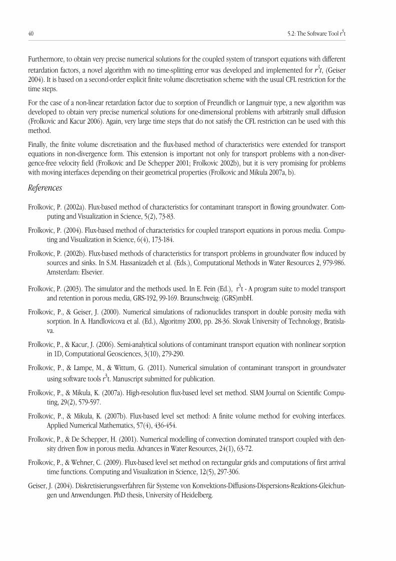
Furthermore, to obtain very precise numerical solutions for the coupled system of transport equations with differentretardation factors, a novel algorithm with no time-splitting error was developed and implemented for r3t, (Geiser2004). It is based on a second-order explicit finite volume discretisation scheme with the usual CFL restriction for thetime steps.

For the case of a non-linear retardation factor due to sorption of Freundlich or Langmuir type, a new algorithm wasdeveloped to obtain very precise numerical solutions for one-dimensional problems with arbitrarily small diffusion(Frolkovic and Kacur 2006). Again, very large time steps that do not satisfy the CFL restriction can be used with thismethod.

Finally, the finite volume discretisation and the flux-based method of characteristics were extended for transportequations in non-divergence form. This extension is important not only for transport problems with a non-diver-gence-free velocity field (Frolkovic and De Schepper 2001; Frolkovic 2002b), but it is very promising for problemswith moving interfaces depending on their geometrical properties (Frolkovic and Mikula 2007a, b).

References

Frolkovic, P. (2002a). Flux-based method of characteristics for contaminant transport in flowing groundwater. Com-puting and Visualization in Science, 5(2), 73-83.

Frolkovic, P. (2004). Flux-based method of characteristics for coupled transport equations in porous media. Compu-ting and Visualization in Science, 6(4), 173-184.

Frolkovic, P. (2002b). Flux-based methods of characteristics for transport problems in groundwater flow induced bysources and sinks. In S.M. Hassanizadeh et al. (Eds.), Computational Methods in Water Resources 2, 979-986.Amsterdam: Elsevier.

Frolkovic, P. (2003). The simulator and the methods used. In E. Fein (Ed.), r3t - A program suite to model transportand retention in porous media, GRS-192, 99-169. Braunschweig: (GRS)mbH.

Frolkovic, P., & Geiser, J. (2000). Numerical simulations of radionuclides transport in double porosity media withsorption. In A. Handlovicova et al. (Ed.), Algoritmy 2000, pp. 28-36. Slovak University of Technology, Bratisla-va.

Frolkovic, P., & Kacur, J. (2006). Semi-analytical solutions of contaminant transport equation with nonlinear sorptionin 1D, Computational Geosciences, 3(10), 279-290.

Frolkovic, P., & Lampe, M., & Wittum, G. (2011). Numerical simulation of contaminant transport in groundwaterusing software tools r3t. Manuscript submitted for publication.

Frolkovic, P., & Mikula, K. (2007a). High-resolution flux-based level set method. SIAM Journal on Scientific Compu-ting, 29(2), 579-597.

Frolkovic, P., & Mikula, K. (2007b). Flux-based level set method: A finite volume method for evolving interfaces.Applied Numerical Mathematics, 57(4), 436-454.

Frolkovic, P., & De Schepper, H. (2001). Numerical modelling of convection dominated transport coupled with den-sity driven flow in porous media. Advances in Water Resources, 24(1), 63-72.

Frolkovic, P., & Wehner, C. (2009). Flux-based level set method on rectangular grids and computations of first arrivaltime functions. Computing and Visualization in Science, 12(5), 297-306.

Geiser, J. (2004). Diskretisierungsverfahren für Systeme von Konvektions-Diffusions-Dispersions-Reaktions-Gleichun-gen und Anwendungen. PhD thesis, University of Heidelberg.

40 5.2: The Software Tool r3t

A5.3: Fractured Porous MediaSabine Stichel, Dmitry Logashenko, Alfio Grillo, Sebastian Reiter, Gabriel Wittum

Simulation of groundwater flow and solute transport in fractured porous media is currently one of the most activeresearch fields and is of great practical importance. Fractures influence flow and transport processes essentially.Espeacially, the often high conductivity in the fractures leads to their representation as preferential fast pathways forcontaminant transport. Because of their long and thin geometry, fractures are difficult to handle numerically: on theone hand, computational grids covering the whole domain where hydrology is simulated usually cannot resolve thethickness of fractures. On the other hand, the simulations on finer grids resolving the fractures even in smallerdomains encounter specific difficulties with numerical solvers that demonstrate poor performance in this case.

Therefore we follow two approaches. In the first one, useful for simulations in large domains with many fractures,we represent the fractures by low-dimensional hypersurfaces. We develop special models based on averaging ofunknowns in the fractures in the direction orthogonal to the fracture surfaces (Grillo et al. 2009a,b,2010a) by emplo-ying an upscaling method exposed in Bear (1979). Initially, the fracture is regarded as a full-dimensional porous me-dium filled by a two-constituent fluid, which consists of water and brine. The equations describing the macroscopicbehaviour of the medium are given by the balance of mass of the contaminant and the fluid-phase as a whole. It isassumed that the fluid-phase velocity and the diffusive mass flux of the contaminant are given by Darcy‘s and Fick‘slaws, respectively. Subsequently, these balance equations are averaged according to a procedure known as “averagealong the vertical” (see Bear 1977). This leads to a set of equations describing an equivalent low-dimensional porous

medium. In order for these equations to be consistent,surface physical quantities (mass density, concentration,velocity and mass flux) have to be introduced, and the vec-tor fields describing Darcy's and Fick's laws have to be pro-jected onto the tangent space of the equivalent lower-di-mensional fracture. The gravity force in the fracture istreated in a special way. It should be also pointed out thatthe normal components of these vector fields account forthe interaction of the fracture with the surrounding medi-um. The explicit determination of the way in which suchan interaction takes place, and its numerical treatment re-quire the self-consistent expression of normal mass fluxes.

Numerically, the low-dimensional hyperfaces arerepresented by so-called degenerated grid elements. Fordiscretisation, the vertex-centered finite volume method,in particular based on the low-dimensional finite volumesin fractures (Grillo et al. 2010a), is used. Conventional nu-merical methods, like Newton iteration with geometricalmultigrid method for linearised equations, demonstratevery good performance for this type of problems.

Figure 1. Simulation of the Henry problem with a fracture: (a) d-dimensional, (b) (d-1)-dimensional

A5.3: Fractured porous media 41

(a) (b)

0

0.1

0.2

0.3

0.4

0.5

0 20 40 60 80 100 0

0.0002

0.0004

0.0006

0.0008

0.001

0.0012

0.0014

0.0016

time T [h]

non-

dimen

siona

l con

cent

ratio

n c f /!

pB

absolute error

Full-dimensionalLow-dimensional

Abs. error

0

0.0005

0.001

0.0015

0.002

0 20 40 60 80 100 0

5e-06

1e-05

1.5e-05

2e-05

2.5e-05

time T [h]

Full-dimensionalLow-dimensional

Abs. error

jump (!

(2) - !

(1) ) absolute error

Figure 2. Comparison of the d- and the (d-1)-dimensional si-mulations: (a) non-dimensional concentrations in the fractu-re, (b) jumps of the non-dimensional concentrations at thefracture interfaces

(a)

(b)

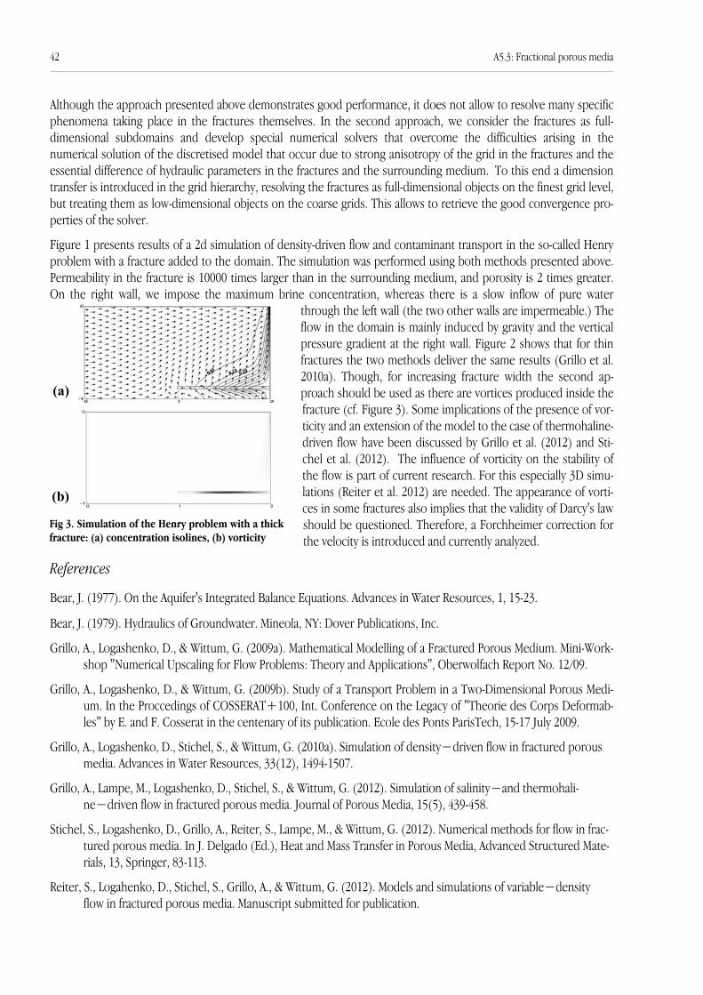
Although the approach presented above demonstrates good performance, it does not allow to resolve many specificphenomena taking place in the fractures themselves. In the second approach, we consider the fractures as full-dimensional subdomains and develop special numerical solvers that overcome the difficulties arising in thenumerical solution of the discretised model that occur due to strong anisotropy of the grid in the fractures and theessential difference of hydraulic parameters in the fractures and the surrounding medium. To this end a dimensiontransfer is introduced in the grid hierarchy, resolving the fractures as full-dimensional objects on the finest grid level,but treating them as low-dimensional objects on the coarse grids. This allows to retrieve the good convergence pro-perties of the solver.

Figure 1 presents results of a 2d simulation of density-driven flow and contaminant transport in the so-called Henryproblem with a fracture added to the domain. The simulation was performed using both methods presented above.Permeability in the fracture is 10000 times larger than in the surrounding medium, and porosity is 2 times greater.On the right wall, we impose the maximum brine concentration, whereas there is a slow inflow of pure water

through the left wall (the two other walls are impermeable.) Theflow in the domain is mainly induced by gravity and the verticalpressure gradient at the right wall. Figure 2 shows that for thinfractures the two methods deliver the same results (Grillo et al.2010a). Though, for increasing fracture width the second ap-proach should be used as there are vortices produced inside thefracture (cf. Figure 3). Some implications of the presence of vor-ticity and an extension of the model to the case of thermohaline-driven flow have been discussed by Grillo et al. (2012) and Sti-chel et al. (2012). The influence of vorticity on the stability ofthe flow is part of current research. For this especially 3D simu-lations (Reiter et al. 2012) are needed. The appearance of vorti-ces in some fractures also implies that the validity of Darcy's lawshould be questioned. Therefore, a Forchheimer correction forthe velocity is introduced and currently analyzed.

References

Bear, J. (1977). On the Aquifer's Integrated Balance Equations. Advances in Water Resources, 1, 15-23.

Bear, J. (1979). Hydraulics of Groundwater. Mineola, NY: Dover Publications, Inc.

Grillo, A., Logashenko, D., & Wittum, G. (2009a). Mathematical Modelling of a Fractured Porous Medium. Mini-Work-shop "Numerical Upscaling for Flow Problems: Theory and Applications", Oberwolfach Report No. 12/09.

Grillo, A., Logashenko, D., & Wittum, G. (2009b). Study of a Transport Problem in a Two-Dimensional Porous Medi-um. In the Proccedings of COSSERAT+100, Int. Conference on the Legacy of "Theorie des Corps Deformab-les" by E. and F. Cosserat in the centenary of its publication. Ecole des Ponts ParisTech, 15-17 July 2009.

Grillo, A., Logashenko, D., Stichel, S., & Wittum, G. (2010a). Simulation of density−driven flow in fractured porousmedia. Advances in Water Resources, 33(12), 1494-1507.

Grillo, A., Lampe, M., Logashenko, D., Stichel, S., & Wittum, G. (2012). Simulation of salinity−and thermohali-ne−driven flow in fractured porous media. Journal of Porous Media, 15(5), 439-458.

Stichel, S., Logashenko, D., Grillo, A., Reiter, S., Lampe, M., & Wittum, G. (2012). Numerical methods for flow in frac-tured porous media. In J. Delgado (Ed.), Heat and Mass Transfer in Porous Media, Advanced Structured Mate-rials, 13, Springer, 83-113.

Reiter, S., Logahenko, D., Stichel, S., Grillo, A., & Wittum, G. (2012). Models and simulations of variable−densityflow in fractured porous media. Manuscript submitted for publication.

42 A5.3: Fractional porous media

(a)

(b)

Fig 3. Simulation of the Henry problem with a thickfracture: (a) concentration isolines, (b) vorticity

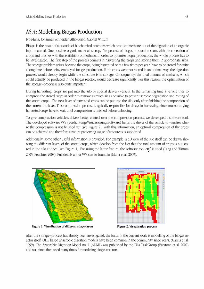
A5.4: Modelling Biogas ProductionIvo Muha, Johannes Schneider, Alfio Grillo, Gabriel Wittum

Biogas is the result of a cascade of biochemical reactions which produce methane out of the digestion of an organicinput material. One possible organic material is crop. The process of biogas production starts with the collection ofcrops and finishes with the availability of methane. In order to optimise biogas production, the whole process has tobe investigated. The first step of the process consists in harvesting the crops and storing them in appropriate silos.The storage problem arises because the crops, being harvested only a few times per year, have to be stored for quitea long time before being employed for gas production. If the crops were not stored in an optimal way, the digestionprocess would already begin while the substrate is in storage. Consequently, the total amount of methane, whichcould actually be produced in the biogas reactor, would decrease significantly. For this reason, the optimisation ofthe storage–process is also quite important.

During harvesting, crops are put into the silo by special delivery vessels. In the remaining time a vehicle tries tocompress the stored crops in order to remove as much air as possible to prevent aerobic degradation and rotting ofthe stored crops. The next layer of harvested crops can be put into the silo, only after finishing the compression ofthe current top layer. This compression process is typically responsible for delays in harvesting, since trucks carryingharvested crops have to wait until compression is finished before unloading.

To give compression vehicle‘s drivers better control over the compression process, we developed a software tool.The developed software VVS (VerdichtungsVisualisierungsSoftware) helps the driver of the vehicle to visualise whe-re the compression is not finished yet (see Figure 2). With this information, an optimal compression of the cropscan be achieved and therefore a nature preserving usage of resources is supported.

Additionally, some other useful information is provided. For example, a 3D view of the silo itself can be drawn sho-wing the different layers of the stored crops, which develop from the fact that the total amount of crops is not sto-red in the silo at once (see Figure 1). For using the latter feature, the software tool ⋲ is used (Lang and Wittum2005; Feuchter 2008). Full details about VVS can be found in (Muha et al. 2009).

After the storage–process has already been investigated, the focus of the current work is modelling of the biogas re-actor itself. ODE based anaerobic digestion models have been common in the community since years, (Garcia et al.1999). The Anaerobic Digestion Model no. 1 (ADM1) was published by the IWA TaskGroup (Batstone et al. 2002)and was since then used many times for modeling biogas reactors.

Figure 1. Visualisation of different silage-layers Figure 2. Visualisation process

A5.4: Modelling Biogas Production 43

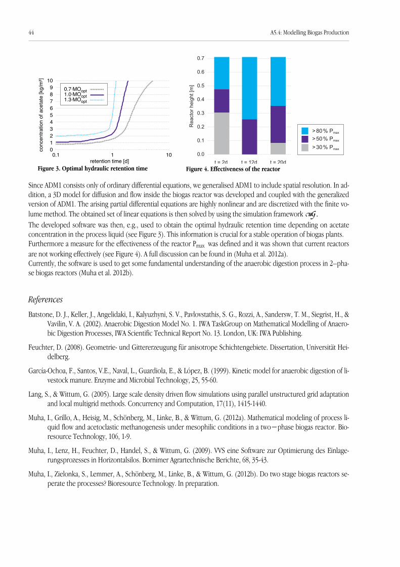
Since ADM1 consists only of ordinary differential equations, we generalised ADM1 to include spatial resolution. In ad-dition, a 3D model for diffusion and flow inside the biogas reactor was developed and coupled with the generalizedversion of ADM1. The arising partial differential equations are highly nonlinear and are discretized with the finite vo-lume method. The obtained set of linear equations is then solved by using the simulation framework ⋲. The developed software was then, e.g., used to obtain the optimal hydraulic retention time depending on acetateconcentration in the process liquid (see Figure 3). This information is crucial for a stable operation of biogas plants.Furthermore a measure for the effectiveness of the reactor Pmax was defined and it was shown that current reactorsare not working effectively (see Figure 4). A full discussion can be found in (Muha et al. 2012a). Currently, the software is used to get some fundamental understanding of the anaerobic digestion process in 2–pha-se biogas reactors (Muha et al. 2012b).

References

Batstone, D. J., Keller, J., Angelidaki, I., Kalyuzhyni, S. V., Pavlovstathis, S. G., Rozzi, A., Sandersw, T. M., Siegrist, H., &Vavilin, V. A. (2002). Anaerobic Digestion Model No. 1. IWA TaskGroup on Mathematical Modelling of Anaero-bic Digestion Processes, IWA Scientific Technical Report No. 13. London, UK: IWA Publishing.

Feuchter, D. (2008). Geometrie- und Gittererzeugung für anisotrope Schichtengebiete. Dissertation, Universität Hei-delberg.

García-Ochoa, F., Santos, V.E., Naval, L., Guardiola, E., & López, B. (1999). Kinetic model for anaerobic digestion of li-vestock manure. Enzyme and Microbial Technology, 25, 55-60.

Lang, S., & Wittum, G. (2005). Large scale density driven flow simulations using parallel unstructured grid adaptationand local multigrid methods. Concurrency and Computation, 17(11), 1415-1440.

Muha, I., Grillo, A., Heisig, M., Schönberg, M., Linke, B., & Wittum, G. (2012a). Mathematical modeling of process li-quid flow and acetoclastic methanogenesis under mesophilic conditions in a two−phase biogas reactor. Bio-resource Technology, 106, 1-9.

Muha, I., Lenz, H., Feuchter, D., Handel, S., & Wittum, G. (2009). VVS eine Software zur Optimierung des Einlage-rungsprozesses in Horizontalsilos. Bornimer Agrartechnische Berichte, 68, 35-43.

Muha, I., Zielonka, S., Lemmer, A., Schönberg, M., Linke, B., & Wittum, G. (2012b). Do two stage biogas reactors se-perate the processes? Bioresource Technology. In preparation.

Figure 3. Optimal hydraulic retention time Figure 4. Effectiveness of the reactor

44 A5.4: Modelling Biogas Production

0 1 2 3 4 5 6 7 8 9

10

0.1 1 10

conc

entra

tion

of a

ceta

te [k

g/m

³]

retention time [d]

0.7!MOopt1.0!MOopt1.3!MOopt

> 30 % Pmax

> 50 % Pmax

> 80 % Pmax

t = 2d

Rea

ctor

hei

ght [

m]

0.7

0.6

0.5

0.4

0.3

0.2

0.1

0.0t = 20dt = 12d

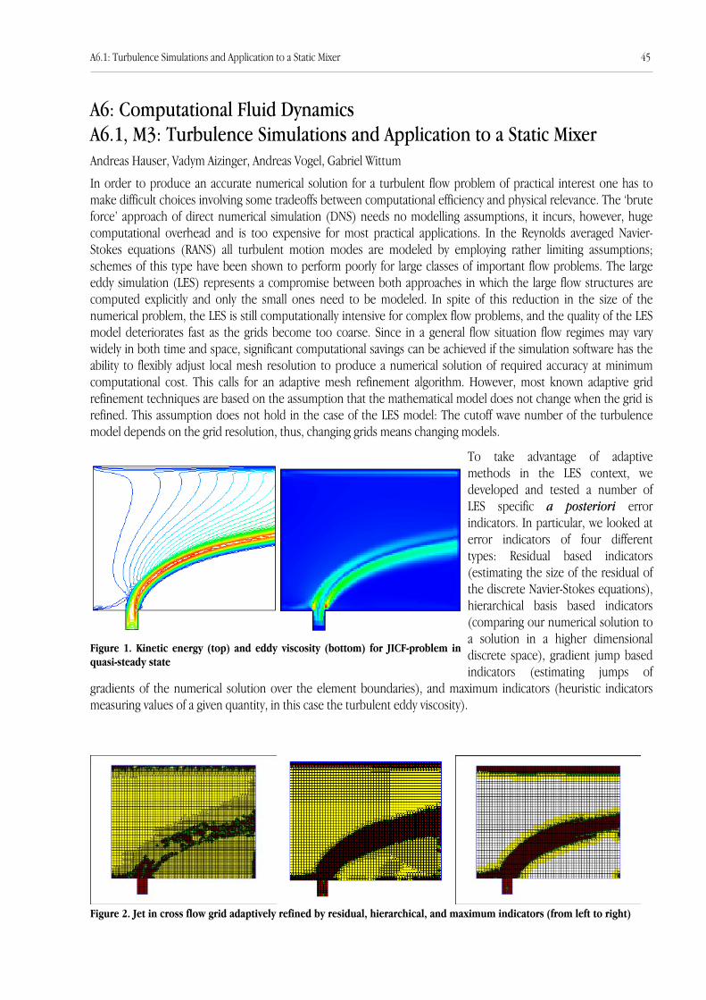
A6: Computational Fluid DynamicsA6.1, M3: Turbulence Simulations and Application to a Static MixerAndreas Hauser, Vadym Aizinger, Andreas Vogel, Gabriel Wittum

In order to produce an accurate numerical solution for a turbulent flow problem of practical interest one has tomake difficult choices involving some tradeoffs between computational efficiency and physical relevance. The ‘bruteforce’ approach of direct numerical simulation (DNS) needs no modelling assumptions, it incurs, however, hugecomputational overhead and is too expensive for most practical applications. In the Reynolds averaged Navier-Stokes equations (RANS) all turbulent motion modes are modeled by employing rather limiting assumptions;schemes of this type have been shown to perform poorly for large classes of important flow problems. The largeeddy simulation (LES) represents a compromise between both approaches in which the large flow structures arecomputed explicitly and only the small ones need to be modeled. In spite of this reduction in the size of thenumerical problem, the LES is still computationally intensive for complex flow problems, and the quality of the LESmodel deteriorates fast as the grids become too coarse. Since in a general flow situation flow regimes may varywidely in both time and space, significant computational savings can be achieved if the simulation software has theability to flexibly adjust local mesh resolution to produce a numerical solution of required accuracy at minimumcomputational cost. This calls for an adaptive mesh refinement algorithm. However, most known adaptive gridrefinement techniques are based on the assumption that the mathematical model does not change when the grid isrefined. This assumption does not hold in the case of the LES model: The cutoff wave number of the turbulencemodel depends on the grid resolution, thus, changing grids means changing models.

To take advantage of adaptivemethods in the LES context, wedeveloped and tested a number ofLES specific a posteriori errorindicators. In particular, we looked aterror indicators of four differenttypes: Residual based indicators(estimating the size of the residual ofthe discrete Navier-Stokes equations),hierarchical basis based indicators(comparing our numerical solution toa solution in a higher dimensionaldiscrete space), gradient jump basedindicators (estimating jumps of

gradients of the numerical solution over the element boundaries), and maximum indicators (heuristic indicatorsmeasuring values of a given quantity, in this case the turbulent eddy viscosity).

A6.1: Turbulence Simulations and Application to a Static Mixer 45

Figure 1. Kinetic energy (top) and eddy viscosity (bottom) for JICF-problem inquasi-steady state

Figure 2. Jet in cross flow grid adaptively refined by residual, hierarchical, and maximum indicators (from left to right)

The grid adaptivity algorithms were applied to the well known jet-in-crossflow (JICF) problem in the configurationshown in Figure 1. In this setting, a fast jet of fluid exiting an orifice interacts with the ambient fluid moving in cross-wise direction. Figure 2 illustrates adaptively refined grids produced with the help of the residual, hierarchical basis,and maximum indicators. An evaluation of the modelling and discretisation components of error lead to a conclusionthat the residual based indicator performs best of all tested error indicators.

An important application of advanced numerical techniques developed for incompressible flow is a static mixerproblem where two or more fluids are mixed solely by the combined effect of advection and turbulence induced bythe mixer geometry. This problem requires an additional equation to represent transport and mixing of a passivetracer. Simulation results were compared to the experiments performed by the group of Prof. Thévenin at theUniversity of Magdeburg. Figure 3 illustrates the mixer geometry and the experimental setup.

One of the most important goals of this simulation was toreproduce experimental values of mixing quality indicatorssuch as temporal or spatial mixing efficiency. It turned outthat even on those grids that were too coarse to resolve fineflow and mixing structures the values of mixing indicatorsdownstream from the highly turbulent zone right after themixer were reasonably close in both, experimental andnumerical cases. A comparison of the spatial efficiency(SMD) indices of the experimental measurements vs.laminar and turbulent numerical simulations is given inFigure 4. To improve the representation of mixing in thehighly turbulent zone right after the mixer an adaptive meshrefinement scheme customised for mixing simulationsappears to be a very promising avenue of further research.

References

Aizinger, V., Hauser, A., Wittum, G. (2010). Simulation of Flow and Transport in a Static Mixer Using Adaptive andHigher Order Numerical Methods. In H. Bockhorn et al. (Eds.), Heat and Mass Transfer, Micro and Macro Mi-xing: analysis, simulation and numerical calculation (pp. 245-262). Berlin: Springer

Gordner, A., Nägele, S., & Wittum, G. (2006). Multigrid methods for large-eddy simulation. In W. Jäger et al. (Eds.),Reactive Flows, Diffusion and Transport. Berlin: Springer.

Hauser, A., Wittum, G. (2006). Parallel Large Eddy Simulation with UG. High Performance Computing in Science andEngineering '06. Berlin: Springer.

Hauser, A., Wittum, G. (2008). Analysis of Uniform and Adaptive LES in Natural Convection Flow. In J. Meyers et al.(Eds.), Quality and Reliability of Large-Eddy Simulations (pp. 105-116). Dordrecht: Springer.

Figure 4. Comparison of spatial mixing efficiency index inthe xy-plane cut after the mixer

46 A6.1: Turbulence Simulations and Application to a Static Mixer

Figure 3. Side view of the static mixer (left), experimental setup (right)

A6.2: Discontinuous Galerkin Method for Incompressible Navier-StokesEquationsVadym Aizinger, Gabriel Wittum

A high order adaptive numerical scheme for the incompressibleNavier-Stokes equations is the ultimate goal of our work withthe Discontinuous Galerkin (DG) method. A discretisationbased on this method was developed and fully integrated in theUG package, including the time stepping algorithms as well asnon-linear and linear solvers. A series of benchmarking testscomparing the performance and cost of the DG implementationto the node-centred second order Finite Volume solver (ourstandard package for the incompressible Navier-Stokes equa-tions) produced encouraging results showing expectedefficiency gains connected with the high order scheme. In particular, we simulated flow in a 2D driven cavity with Re=10000. Figure 1 provides a comparison of vertical and horizontalmidline velocity profiles for different grid levels anddiscretisations. These plots confirm that for large flow featureshigh order numerical solutions can be more accurate on farcoarser meshes than the standard Finite Volume method: E.g.,compare the fourth order DG solution at grid level 2 (64elements, 960 degrees of freedom) to the Finite Volumesolution at grid level 5 (4096 elements, 2113 degrees offreedom). The advantages of high order methods appear to beless pronounced though when resolving small flow features.This situation is due to the fact that the element size must be atleast comparable to the size of the simulated flow structures inorder to be able to properly represent them.

To test the Discontinuous Galerkin solver on a morechallenging application we simulated flow (without tracertransport) in the static mixer problem described in section A6.1.Figure 2 compares the averaged axial velocity profiles in a crosssection right after the mixer. The difficulties that were seen inthe driven cavity plots are even more obvious here: The Discontinuous Galerkin results capture well the positionsand the values of extrema, but a coarse grid resolution prevents good representation of fine flow structures, evenmore so in the quadratic case. Fortunately, in addition to a high order discretisation, the Discontinuous Galerkinmethod possesses excellent adaptivity capabilities in grid resolution and approximation order that we plan to put togood use in addressing this issue.

The next test (Figure 3) concerns the power spectra of the axial velocity component at the point located on themain axis of the mixer. The experimental measurements (peak at ~0.36 Hz) agree rather well with the Finite Vol-ume results, but both DG frequencies are a bit off: ~ 0.4 for the piecewise linear approximation on level 3 and~0.43 for the piecewise quadratic approximation on level 2. One possible explanation is the absence of an LESmodel in our DG implementation resulting in an unrealistically low value of the viscosity term.

A6.2: Discontinuous Galerkin Method 47

Figure 1. x-velocity at x=0.5(left) and y-velocityat y=0.5(right) for driven cavity flow with Re=10000

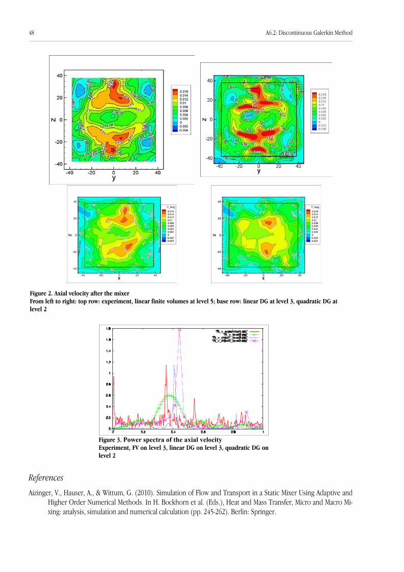
References

Aizinger, V., Hauser, A., & Wittum, G. (2010). Simulation of Flow and Transport in a Static Mixer Using Adaptive andHigher Order Numerical Methods. In H. Bockhorn et al. (Eds.), Heat and Mass Transfer, Micro and Macro Mi-xing: analysis, simulation and numerical calculation (pp. 245-262). Berlin: Springer.

48 A6.2: Discontinuous Galerkin Method

Figure 3. Power spectra of the axial velocityExperiment, FV on level 3, linear DG on level 3, quadratic DG onlevel 2

Figure 2. Axial velocity after the mixerFrom left to right: top row: experiment, linear finite volumes at level 5; base row: linear DG at level 3, quadratic DG atlevel 2

A6.3: Multiphase FlowsPeter Frolkovič, Dmitry Logashenko, Christian Wehner, Gabriel Wittum

One of the most active research fields in computational fluid dynamics is the numerical simulation of incompressibletwo-phase flow. This great interest has contributed to the development of many, often substantially different nume-rical methods for this kind of problems. One of them is based on the level set formulation in which the interface bet-ween two phases is represented implicitly by the zero level set of a smooth function (see also Section M4). This ap-proach is easier to handle than other methods, that use a direct representation of the dynamic interface (e.g. La-grangian-type methods, moving grids).

The flux-based level set method for two-phase flow we developed (Frolkovič et al. 2008, Frolkovič et al. 2010) uses asharp treatment of the numerical interface and requires no artificial post-processing steps for stable behavior. In nu-merical test examples computed with ⋲, it showed good mass conservation properties and negligible parasite cur-rents.

The method applies analogous finite volume discretisati-ons to the local balance formulations for the conservationof momentum, mass and level sets on identical vertex-centered control volumes. To enable the sharp treatmentof the interface condition in the method, we extend theapproximation spaces for the pressure and the velocity byadditional degrees of freedom for the elements intersec-ted by the interface. This method can be implemented bya relatively simple extension of an existing finite volumediscretisation for the single-phase Navier-Stokes equati-ons. In our case, we used the collocated discretisationfrom Nägele and Wittum (2007). As discretisation methodfor the level set equation we use the flux-based level setmethod (Frolkovič and Mikula 2007).

t=0 t=0.0175s t=0.125s t=0.25s

7e-4

1e-3

1.4e-3

1.9e-3

2.6e-3

33 x 49 65 x 97 129 x 193 257 x 385

area

erro

r [cm

x c

m]

nr of gridpoints

Figure 1. Evolution of a rising bubble in counterflow

Figure 2. Error in the volume of the bubble at time t=0.25 on different grids for the experiment depictedin Figure 1

A6.3: Multiphase Flows 49

The approximation of the curvature is computed using quadratic inter-polation of the level set function on a refined grid. In each time step, werefine only the elements that are near or at interface and use this locallyrefined grid only for the numerical solution of the level set equation.

It is common, to use a signed distance function as initial level set func-tion, that means a distance function for the interface with negative signin the inside region and positive sign outside. In general, the level setfunction can develop very steep or flat gradients in the region aroundthe interface during computation. This causes essential difficulties innumerical computations, e.g., inaccurate computation of the curvature.To avoid this, it is reasonable to replace the level set function at certaintime steps with a signed distance function, that has the same zero levelset. This "reinitialisation" process is done by solving a reinitialisationequation using the flux-based level set method.

Numerical tests confirmed convergence and stability of the describedmethod. For sufficiently fine grids, grid-independent numerical soluti-ons for the tested problems were obtained. The test problem illustratedin figure 1 is the simulation of a rising bubble in counterflow. Thedensity is set to 0.995 g/cm³ outside the bubble and 0.001107 g/cm³ in-side, the viscosity is set to 0.104 dyn s/cm² outside and 0.048 dyn s/cm²inside, the surface tension factor is set to 2 dyn/cm and the gravitationconstant is 980 cm/s². A parabolic profile of the inflow velocity is prescri-bed as boundary condition on the top (the maximum velocity is 4 cm/s), zero velocities are prescribed on the left and right side and on the lo-wer side a zero stress outflow-boundary condition is used. Initially, the bubble is a circle with radius R=0.175 cm. During the computation,the bubble is pressed upwards due to gravitation, but at the same time, the incoming fluid hinders the bubble tomove up. Although the interface is deformed, the volume of the bubble should remain constant.

Numerical mass conservation is not guaranteed by the level set formulation, so conservation of mass is an importantissue for two-phase flow level set methods. In Figure 2, the mass conservation error observed on different grid levelsfor the test problem at time t=0.25 is plotted, we note convergence to zero with first order of accuracy.

Figure 3 presents an analogous test case of a rising bubble in a cylinder in three dimensions.

References

Frolkovič, P., Logashenko, D., Wehner, C., & Wittum, G. (2010). Finite volume method for two-phase flows usinglevel set formulation. Preprint 2010-10, Department of Mathematics and Descriptive Geometry, Slovak Univer-sity of Technology, Bratislava 2010.

Frolkovič, P., Logashenko, D., & Wittum, G. (2008). Flux-based level set method for two-phase flows. In R. Eymard, J.-M. Herard (Eds.), Finite Volumes for Complex Applications V (pp. 415-422). London: ISTE and Wiley.

Frolkovič, P., & Mikula, K. (2007). High-resolution flux-based level set method. SIAM Journal on Scientific Compu-ting, 29(2), 579–597.

Nägele, S., & Wittum, G. (2007). On the influence of different stabilisation methods for the incompressible Navier-Stokes equations. Journal of Computational Physics, 224(1), 100–116.

Figure 3. Simulation of a rising bubble in 3D

50 A6.3: Multiphase Flows

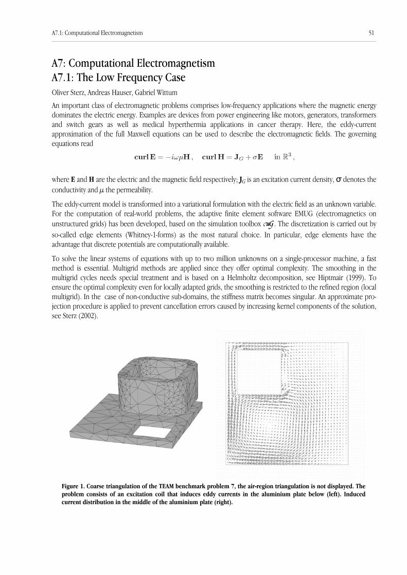
A7: Computational ElectromagnetismA7.1: The Low Frequency CaseOliver Sterz, Andreas Hauser, Gabriel Wittum

An important class of electromagnetic problems comprises low-frequency applications where the magnetic energydominates the electric energy. Examples are devices from power engineering like motors, generators, transformersand switch gears as well as medical hyperthermia applications in cancer therapy. Here, the eddy-currentapproximation of the full Maxwell equations can be used to describe the electromagnetic fields. The governingequations read

where E and H are the electric and the magnetic field respectively; JG is an excitation current density, σ denotes theconductivity and µ the permeability.

The eddy-current model is transformed into a variational formulation with the electric field as an unknown variable.For the computation of real-world problems, the adaptive finite element software EMUG (electromagnetics onunstructured grids) has been developed, based on the simulation toolbox ⋲. The discretization is carried out byso-called edge elements (Whitney-1-forms) as the most natural choice. In particular, edge elements have theadvantage that discrete potentials are computationally available.

To solve the linear systems of equations with up to two million unknowns on a single-processor machine, a fastmethod is essential. Multigrid methods are applied since they offer optimal complexity. The smoothing in themultigrid cycles needs special treatment and is based on a Helmholtz decomposition, see Hiptmair (1999). Toensure the optimal complexity even for locally adapted grids, the smoothing is restricted to the refined region (localmultigrid). In the case of non-conductive sub-domains, the stiffness matrix becomes singular. An approximate pro-jection procedure is applied to prevent cancellation errors caused by increasing kernel components of the solution,see Sterz (2002).

A7.1: Computational Electromagnetism 51

Figure 1. Coarse triangulation of the TEAM benchmark problem 7, the air-region triangulation is not displayed. Theproblem consists of an excitation coil that induces eddy currents in the aluminium plate below (left). Inducedcurrent distribution in the middle of the aluminium plate (right).

The software EMUG has been successfully employed for benchmark problems (see Figure 1) as well as realisticapplications (see Figure 2). A parallel prototype of the electromagnetic simulation tool is currently being developed.

From the known fields and currents, force densities and Ohmic losses can easily be computed. The Ohmic lossesgive rise to heat generation in the conductors. In order to compute the temperatures in general cooling, effects offluid flow, diffusion and radiation must be considered. This will lead to coupled problems of electromagnetics andheat transfer (multiphysics) since the conductivity depends on the temperature.

References

Hiptmair, R. (1999). Multigrid method for Maxwell’s equations. SIAM Journal on Numerical Analalysis, 36(1),204–225.

Hiptmair, R. & Sterz, O. (2003). Current and voltage excitations for the eddy current model. Eidgenössische Techni-sche Hochschule, Research report / Seminar für Angewandte Mathematik No. 2003-07.

Sterz, O. (2002). Multigrid for time harmonic eddy currrents without gauge. In Scientific Computing in ElectricalEngineering. Proceedings of the 4th International Workshop Scientific Computing in Electrical Engineering,Eindhoven, The Netherlands, June 23–28, LNCSE. Berlin: Springer.

Sterz, O. (2003). Modellierung und Numerik zeitharmonischer Wirbelstromprobleme in 3D. Whitney- Elemente,adaptive Mehrgitterverfahren, Randelemente. Dissertation, Universität Heidelberg.

Sterz, O., Hauser, A., & Wittum, G. (2006). Adaptive Local Multigrid Methods for the Solution of Time Harmonic EddyCurrent Problems. IEEE Transactions on Magnetics, 42(2), 309-318.

52 A7.1: Computational Electromagnetism

Figure 2. Magnitude of the magnetic field in a gas-insulated switch gear along different cutting planes

A8: Reduction of Numerical Sensitivities in Crash SimulationsRaphael Prohl, Alfio Grillo, Gabriel Wittum

The simulations of crash tests are very sensitive numerical procedures, which require very accurate and robust algo-rithms in order to handle numerical instabilities. In addition to these, also physical instabilities, which may be due,for example, to the bifurcation behavior of the material under asymmertic loading, have to be detected and correctlytreated by the numerical procedures in order to obtain reliable results. In this context, our task in the project "HPC-10 Reduzierung numerischer Sensitivitäten in der Crashsimulation auf HPC-Rechnern" is to identify and eliminatenumerical instabilities and improve the mathematical analysis of the physical ones.

In a first step we started with the examination of the stability of some algorithms taken from the industry, where full-vehicle-models are normally used. We reduced these models in order to investigate their main features and dealedwith formulating an appropriate mathematical model of a crash test. To this end we considered a non-linear materialbehavior for large elastic and plastic strains. This led to a non-linear system of partial differential equations coupledwith an evolution law for plastic distortions. The latter law was expressed through a plastic flow rule. We concentrateon geometrical and kinematical non-linearities, non-linear material description, elasto-plastic material description,contact simulations, and their impact on the observed instabilities. To perform contact simulations we closely coo-perate with the group of Prof. R. Krause.

Our mathematical model is based on the introduction of a hyperelastic stored energy function W, so that the secondPiola-Kirchhoff stress tensor reads

.

We adopt the Kröner's multiplicative decomposition of the deformation gradient , where and denote the elastic part of deformation and the plastic distortions, respectively. The crucial step in formulating themodel is the determination of an evolution law for . Initially we used an associative flow rule, which is determi-ned by the principle of maximum plastic dissipation and a flow condition , cf. J.C. Simo and T.J.R. Hughes (1998).By letting , , , and denote body forces, the reference density, the Kirchhoffstress tensor, the plastic Cauchy-Green strain tensor and the elastic finger tensor, respectively, the equations to besolved are (formulated in Lagrangian description):

The model presented above will be extended to a rate-dependent elasto-plastic model, consistent to the work of Mi-cunovic et al. in 2011.

The numerical computations of the quasi-static case are performed by an incremental procedure which contains anon-linear sub-problem in every single incremental step. To treat the governing equations of plasticity, we firstlyadopted the well-established return-mapping-algorithm and the consistent-tangent-method for the linearization the-rein. As remarked in Wieners (2007), this plasticity-algorithm may be turn instable because it computes stresses thatdo not necessarily satisfy the global equilibirum equations. Therefore we developed a new class of solution methodswith better mathematical properties by reviewing the plasticity problem in the context of nonlinear programming.We achieve higher robustness by additionally linearizing the constitutive equations and the governing equations of

Se =!W

!E

F = FeFp Fe Fp

Fp

f

B !0 ! Cp = FTp Fp be = FeF

Te

!DIV(FSe) = !0B

"Cp!1

"t= !2

3# tr[be]F

!1 dev[$ ]

"dev[$ ]"F!T

# # 0, f($) $ 0, #f($) = 0

A8: Reduction of Numerical Sensitivities in Crash Simulations 53

plasticity. Hence, our method is an extension of the algorithm proposed in Wieners (2007) to the case of finite defor-mations.

The implementation of the return-mapping-algorithm for finite deformations in our software framework ⋲ hasbeen tested by some benchmark problems. As a reference for our numerical tests, we used a shear/compression-testof the unit-cube with perfect plastic behavior and the well-documented necking of a circular bar as an example forexponential hardening behavior.

References

Krause, R. (2009). A Non-Smooth Multiscale Method for Solving Frictional Two-Body Contact Problems in 2D and 3D with Multigrid Efficiency. SIAM Journal on Scientific Computing, 31(2), 1399-1423.

Micunovic, M.V., Albertini, C., Grillo, A., Muha, I., Wittum, G., & Kudrjavceva, L. (2011). Two dimensional waves inquasi rate independent viscoplastic materials. Journal of Theoretical and Applied Mechanics, 38(1), 47-74.

Wieners, C. (2007). Nonlinear solution methods for infintesimal perfect plasticity. Journal of Applied Mathematicsand Mechanics, 87(8-9), 643-660.

Figure 1. Unit cube in a shear/compression test Figure 2. Max. Stress at the midpoint of the cube

Figure 3. 1/8th of circular bar in a tensile test Figure 4. Change of necking area in time

54 A8: Reduction of Numerical Sensitivities in Crash Simulations

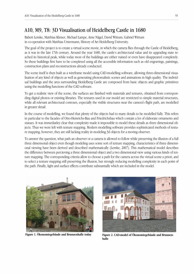
A10, M9, T8: 3D Visualisation of Heidelberg Castle in 1680Babett Lemke, Matthias Kleiser, Michael Lampe, Arne Nägel, David Wittum, Gabriel Wittumin co-operation with Matthias Untermann, History of Art Heidelberg University.

The goal of the project is to create a virtual scene movie, in which the camera flies through the Castle of Heidelberg,as it was in the late 17th century. Around the year 1680, the castle‘s architectural value and its upgrading state re-ached its historical peak, while today most of the buildings are either ruined or even have disappeared completely.So these buildings first have to be completed using all the accessible information such as old engravings, paintings,construction plans and reconstructions already conducted.

The scene itself is then built as a wireframe model using CAD-modelling software, allowing three-dimensional visua-lisation of any kind of objects as well as generating photorealistic scenes and animations in high quality. The individ-ual buildings and the area surrounding Heidelberg Castle are composed from basic objects and graphic primitivesusing the modelling functions of the CAD software.

To get a realistic view of the scene, the surfaces are finished with materials and textures, obtained from correspon-ding digital photos or existing libraries. The textures used in our model are restricted to simple material structures,while all relevant architectural contours, especially the visible structures near the camera's flight path, are modelledin greater detail.

In the course of modelling, we found that plenty of the objects had to many details to be modelled fully. This refersin particular to the facades of Otto-Heinrichs-Bau and Friedrichsbau which contain a lot of elaborate ornaments andstatues. It was immediatley clear that complexity made it impossible to model these details as three dimensional ob-jects. Thus we were left with texture mapping. Modern modelling software provides sophisticated methods of textu-re mapping, however, they are still lacking reality in modeling 3d objects for a moving observer.

To answer the question, what path an observer or a camera is allowed to follow while preserving the illusion of a fullthree dimensonal object even though modeling uses some sort of texture mapping, characteristics of three dimensi-onal viewing have been derived and described mathematically (Lemke, 2007). This mathematical model describesthe difference between percieving a three dimensional object and a two dimensional view using various kinds of tex-ture mapping. The corresponding criteria allow to choose a path for the camera across the virtual scene a priori, andto select a texture mapping still preserving the illusion, but strongly reducing modelling complexity in each point ofthe path. Finally, light and surface effects contribute substantially which are included in the model.

Figure 1. Ökonomiegebäude and Brunnenhalle today Figure 2. CAD-model of Ökonomiegebäude and Brunnen-halle

A10: Visualisation of the Heidelberg Castle in 1680 55

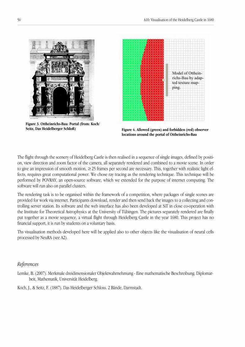
The flight through the scenery of Heidelberg Castle is then realised in a sequence of single images, defined by positi-on, view direction and zoom factor of the camera, all separately rendered and combined to a movie scene. In orderto give an impression of smooth motion, ≥25 frames per second are necessary. This, together with realistic light ef-fects, requires great computational power. We chose ray tracing as the rendering technique. This technique will beperformed by POVRAY, an open-source software, which we extended for the purpose of internet computing. Thesoftware will run also on parallel clusters.

The rendering task is to be organised within the framework of a competition, where packages of single scenes areprovided for work via internet. Participants download, render and then send back the images to a collecting and con-trolling server station. Its software and the web interface has also been developed at SiT in close co-operation withthe Institute for Theoretical Astrophysics at the University of Tübingen. The pictures separately rendered are finallyput together as a movie sequence, a virtual flight through Heidelberg Castle in the year 1680. This project has nofinancial support, it is run by students on a voluntary basis.

Ths visualisation methods developed here will be applied also to other objects like the visualisation of neural cellsprocessed by NeuRA (see A2).

References

Lemke, B. (2007). Merkmale dreidimensionaler Objektwahrnehmung - Eine mathematische Beschreibung. Diplomar-beit, Mathematik, Universität Heidelberg.

Koch, J., & Seitz, F. (1887). Das Heidelberger Schloss. 2 Bände, Darmstadt.

56 A10: Visualisation of the Heidelberg Castle in 1680

Figure 3. Ottheinrichs-Bau: Portal (from: Koch/Seitz, Das Heidelberger Schloß) Figure 4. Allowed (green) and forbidden (red) observer

locations around the portal of Ottheinrichs-Bau

Model of Otthein-richs-Bau by adap-ted texture map-ping.

A11: Computational Acoustics: Eigenmodes of Musical InstrumentsMartin Rupp, Gabriel Wittum

What determines the sound of a guitar? A string can vibrate with all natural multiples of its fundamental frequency.The fundamental frequency is also called the first harmonic overtone, the second harmonic overtone is twice thefundamental frequency and so on. It is the amplitude of the first ten harmonic overtones which characterise thetone. A vibrating string alone hardly produces any audible sound at all, so all string instruments (like the guitar orthe piano) need resonance bodies. When a string is excited, the vibration is carried over to the resonance body,which, due to its larger area, makes the vibration audible.

However, these resonance bodies have resonance frequencies, so the amplification is not independent of the fre-quency: Frequencies close to a resonance frequency will be amplified more than others, but do also fade away faster,because the resonance body drains more energy from the vibrating string resulting in a higher damping of this fre-quency. In other words: The amplitudes of the overtones of a vibrating string are filtered by the resonance body.This also supports Schumann‘s theory of the so-called “formants”, i.e. amplitudes of overtones (Schumann 1929): Anovertone is amplified stronger than others if its frequency lies in a frequency range which is characteristic for an in-strument, independent from the fundamental frequency of the tone or the order of the overtone (when played withthe same intensity).

We started studying the top plate of a guitar. This is the first step towards characterizing the formants of this instru-ment by computation. The elasticity of the top plate is modeled by linear elasticity, so we get a system of partial dif-ferential equations. Because wood has different strength (elasticity coefficients) in the direction from the roots tothe top, from the inner to the outer annual rings, and tangential to the annual rings, we get an anisotropic elasticitytensor.

In our approach, we directly used a full three-dimensional model, because we want to study the three-dimensionaleffect of the bracings of the top plate. Bracings are wooden sticks glued to the top and the back plate to support thelarge free thin surface area of the plates. Since they allow the resonance body to be larger and thinner, and thereforethe guitar to be louder, they can be found in every guitar since the introduction of the traditional fan-bracing by An-tio de Torres Juan in the 19th century. The top plate is over 30 cm long and wide, but only around 2 mm thick (Figu-re 1), resulting in a very challenging geometry.

The discretisation is done by finite elements. The computation of resonance frequencies of the resulting systemleads to a generalised eigenvalue problem Ax =λBx. The eigenvectors with the smallest eigenvalues correspond to

Figure 1. Simple geometry for the guitar top plate Figure 2. Experimental results from Molin/Stetson (Jansson1983)

A11: Computational Acoustics 57

the eigenmodes with the lowest frequency. We are interested in the five to six eigenmodes with lowest frequency.We solve these eigenvalue problems with a special kind of projection method, the Local Optimal Block Preconditio-ned Gradient (LOBPCG) Method, introduced in 2001 by Knyazev. With this method, we can calculate several eigenva-lues at once. Another advantage of LOBPCG is that it does not need much space in computer memory.

As the name LOBPCG suggests, we need to precondition it, that means, we have to find a approximate solution x ofthe linear equation system Ax = b. For this purpose we use an Algebraic Multigrid (AMG) Method, since geometricmultigrid is not able to cope with the highly anisotropic nature of the discretisation matrix A, which results from theanisotropic geometry and the anisotropic elasticity tensor of wood. Another problem is the large number of freeboundaries: Since the top plate is only clamped at the outer edges, the top and the bottom are free boundaries. Thiscauses problems with standard AMG methods, so we chose to use the Filtering Algebraic Multigrid (FAMG) methodintroduced by Christian Wagner in 2000. This AMG method is especially advantageous for linear elasticity problemswith large number of free boundaries.

In our work (Rupp 2009), we calculated the eigenmodes of the guitar top plate without bracings (Figure 3), andfound reasonable agreement with the results from Jansson (1983; Figure 2), although the results show that the influ-ence of the bracings cannot be neglected. In the next step, we will incorporate bracings in our model, and, in a laterone, the coupling with the air inside the guitar. We also studied the behaviour of LOBPCG and similar algorithms de-pending on the strength of the preconditioner and how far “backwards” the algorithm may look, showing that forhard problems (in terms of solving the system Ax = b), the calculation is faster when the algorithm may look fartherbehind, whereas for easy problems, it can be beneficial to do this only for the last eigenvalues.

References

Jansson, E. V. (1983). Function: construction and quality of the guitar. Papers given at a seminar organised by theCommitee for the Acoustics of Music, Royal Swedish Academy of Music, Stockholm.

Knyazev, A. V. (2001). Toward the Optimal Preconditioned Eigensolver: Locally Optimal Block Preconditioned Conju-gate Gradient Method. SIAM Journal of Scientific Computing, 23(2), 517-541.

Nägel A., Falgout R. D., & Wittum G. (2008). Filtering algebraic multigrid and adaptive strategies. Computing and Vi-sualization in Science, 11(3), 159-167.

Schumann, E. (1929). Physik der Klangfarben. Habilitationsschrift, Universität Berlin.

Rupp, M. (2009). Berechnung der Resonanzschwingungen einer Gitarrendecke. Diplomarbeit, Fakultät Mathematik,Universität Heidelberg.

Wagner C. (2000). On the algebraic construction of multilevel transfer operators. Computing, 65(1), 73-95.

58 A11: Computational Acoustics

Figure 3. Results of our simulation, first (177 Hz) and second (200 Hz) eigenmode of the guitar top plate

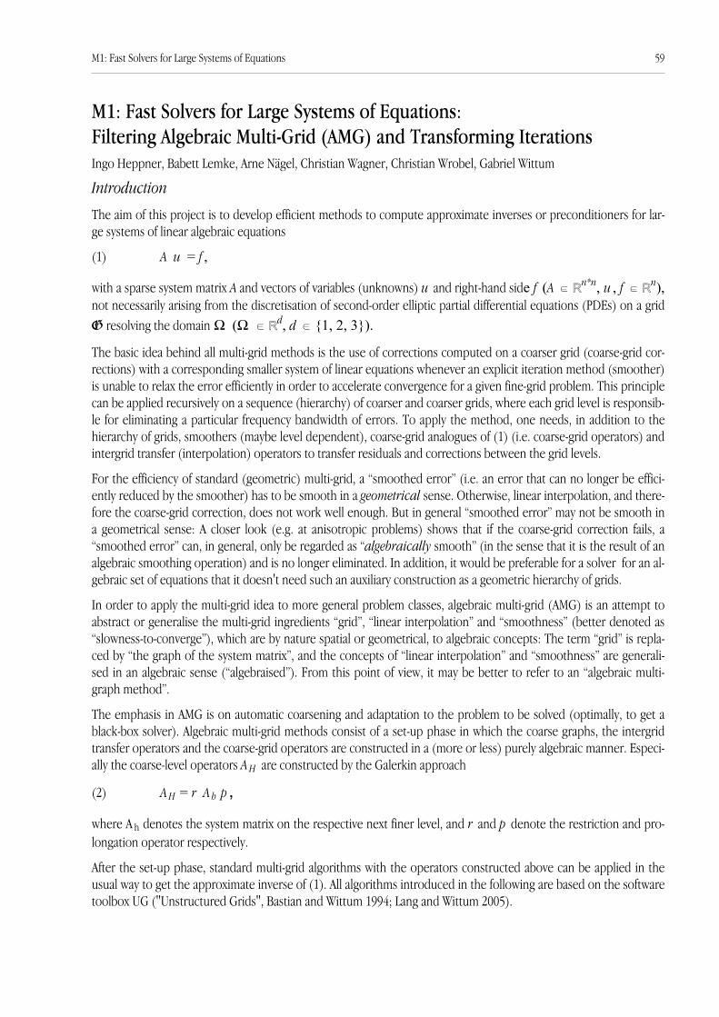
M1: Fast Solvers for Large Systems of Equations: Filtering Algebraic Multi-Grid (AMG) and Transforming IterationsIngo Heppner, Babett Lemke, Arne Nägel, Christian Wagner, Christian Wrobel, Gabriel Wittum

Introduction

The aim of this project is to develop efficient methods to compute approximate inverses or preconditioners for lar-ge systems of linear algebraic equations

(1) A u = f ,

with a sparse system matrix A and vectors of variables (unknowns) u and right-hand side f (A ˝ Rn*n, u , f ˝ Rn),not necessarily arising from the discretisation of second-order elliptic partial differential equations (PDEs) on a gridG resolving the domain „ („ ˝ Rd, d ˝ {1, 2, 3}).

The basic idea behind all multi-grid methods is the use of corrections computed on a coarser grid (coarse-grid cor-rections) with a corresponding smaller system of linear equations whenever an explicit iteration method (smoother)is unable to relax the error efficiently in order to accelerate convergence for a given fine-grid problem. This principlecan be applied recursively on a sequence (hierarchy) of coarser and coarser grids, where each grid level is responsib-le for eliminating a particular frequency bandwidth of errors. To apply the method, one needs, in addition to thehierarchy of grids, smoothers (maybe level dependent), coarse-grid analogues of (1) (i.e. coarse-grid operators) andintergrid transfer (interpolation) operators to transfer residuals and corrections between the grid levels.

For the efficiency of standard (geometric) multi-grid, a “smoothed error” (i.e. an error that can no longer be effici-ently reduced by the smoother) has to be smooth in a geometrical sense. Otherwise, linear interpolation, and there-fore the coarse-grid correction, does not work well enough. But in general “smoothed error” may not be smooth ina geometrical sense: A closer look (e.g. at anisotropic problems) shows that if the coarse-grid correction fails, a“smoothed error” can, in general, only be regarded as “algebraically smooth” (in the sense that it is the result of analgebraic smoothing operation) and is no longer eliminated. In addition, it would be preferable for a solver for an al-gebraic set of equations that it doesn't need such an auxiliary construction as a geometric hierarchy of grids.

In order to apply the multi-grid idea to more general problem classes, algebraic multi-grid (AMG) is an attempt toabstract or generalise the multi-grid ingredients “grid”, “linear interpolation” and “smoothness” (better denoted as“slowness-to-converge”), which are by nature spatial or geometrical, to algebraic concepts: The term “grid” is repla-ced by “the graph of the system matrix”, and the concepts of “linear interpolation” and “smoothness” are generali-sed in an algebraic sense (“algebraised”). From this point of view, it may be better to refer to an “algebraic multi-graph method”.

The emphasis in AMG is on automatic coarsening and adaptation to the problem to be solved (optimally, to get ablack-box solver). Algebraic multi-grid methods consist of a set-up phase in which the coarse graphs, the intergridtransfer operators and the coarse-grid operators are constructed in a (more or less) purely algebraic manner. Especi-ally the coarse-level operators A H are constructed by the Galerkin approach

(2) A H = r A h p ,

where A h denotes the system matrix on the respective next finer level, and r and p denote the restriction and pro-longation operator respectively.

After the set-up phase, standard multi-grid algorithms with the operators constructed above can be applied in theusual way to get the approximate inverse of (1). All algorithms introduced in the following are based on the softwaretoolbox UG ("Unstructured Grids", Bastian and Wittum 1994; Lang and Wittum 2005).

M1: Fast Solvers for Large Systems of Equations 59

Automatic Coarsening (AC)

In many scientific and engineering applications, the spatial objects under consideration have very complicated sha-pes containing a huge number of geometrical details on different scales. AC (Feuchter et al. 2003) is a multi-grid sol-ver for the discretisation of partial differential equations on such complicated domains. As input the algorithm onlyrequires a given grid, fine enough to resolve such complicated shapes, and the discretisation on this grid, instead of ahierarchy of discretisations on coarser grids. In a set-up phase, these coarse auxiliary grids are generated in a black-box fashion trying to resemble the structure of the given grid, i.e. its “element density”, and are used to define purelyalgebraic intergrid transfer and coarse-grid operators. This adaptation process results in a stack of geometrically nes-ted auxiliary grids Gi ¸ „, i = 0, . . . , l max.

Thus, to a certain extent this approach is similar to AMG: for a given fine grid, a hierarchy of coarser grids is created.However, this is not in the spirit of algebraic multi-level approaches since there is no matrix dependence, neither ofcoarse grid selection nor of building the intergrid transfer and coarse grid operators. Also, as opposed to AMG, thecoarsening process does not proceed from the given fine grid towards increasingly coarser grids but an adaptationprocess moves from a very coarse grid towards the given fine grid(s). This approach can therefore be called “semi-al-gebraic”.

Since a naive implementation of this accommodation process would require a lot of search operations with comple-xity O (N 2) (N being the number of elements in the given grid), we utilise a quadtree data structure for a far bettercomplexity of O (j ) (j being the number of levels), accelerating the set-up phase significantly.

Schur-complement multi-grid (SchurMG)

The Schur-complement multi-grid method was constructed as a robust multi-grid method for the interface problemarising from the discretisation of the convection-diffusion equation with strongly discontinuous coefficients ingroundwater flow (Wagner et al. 1997). It is based on an idea by Reusken (Reusken 1994). These and the coarse gridoperators are matrix dependent, but the coarse-grid selection is not (as in AC), so that this method can also be called“semi-algebraic”. The coarse-grid selection of the fine grid and the reordering of the vector of unknowns u (and alsoof right-hand side vector f) so that all variables belonging to fine-grid points and all variables belonging to coarse-gridpoints are blocked and consecutive, induces a 2 x 2 block structure of the system matrix A. Block factorisation thenleads to inverses of the fine-fine block and the Schur complement which would provide the solution in one step ifcomputed exactly. Since the matrix is neither sparse nor easy to invert, one has to approximate the system matrix(lumping) to get a recursively applicable method. One can show that the Schur complement of the modified systemmatrix corresponds to the Galerkin approach with appropriate intergrid transfer operators.

Standard AMG

The set-up phase of the classical AMG method, in the following called RSAMG, as introduced in the fundamental pa-per (Ruge and Stüben 1987), is based on the concept of “strong coupling” and the notion of “slow-to-converge” er-ror which guide the automatic coarsening process and the construction of appropriate intergrid transfer operators toensure that each fine variable is well interpolated from a (small) subset of coarse variables. Coarse-grid equations areconstructed by the Galerkin approach.

Here, a variable vi is said to be “strongly connected to” another variable vj from its neighbourhood if for a fixed para-meter √ (0 < √ ≤ 1):

(3) |aij| ≥ √ maxl≠i (|ail|).

The aim of the coarsening process is that each fine variable has at least one strong coupling to a coarse variable toachieve good interpolation and that there is, as far as possible, no pair of coarse variables that are strongly connectedto each other (i.e. coarse variables should form a maximal independent set) to limit the size of the coarse grid andthus the work which has to be done on it. The interpolation weights are then determined via the solution of the resi-dual equation for an error variable.

60 M1: Fast Solvers for Large Systems of Equations

Filtering and Filtering Algebraic Multigrid

Filtering is another technique for solving linear systems Ax = b. It is based on the filtering property: Find an appro-ximate inverse M, such that:

M t = A t , t ˝ T with a “testing space” T ,

yielding a linear iteration of the type

x new = x old – M –1(A x old – b ).

Depending on T, the resulting method can be tailored to be a smoother or a corrector as described in (Wittum1992). It is possible to derive the filtering space T adaptively during the iteration by Adaptive Filtering (Wagner andWittum 1997). The efficiency of the filtering approach was demonstrated in these papers. However, only so-called fil-tering decompositions were available to construct filters. These are based on block incomplete decompositions andthus are limited to structured grids only. We continued this development with the two-frequency decompositions(Logaschenko 2003; Buzdin and Wittum 2004; Buzdin et al. 2008).

In order ro generalise this method to unstructured grids Filtering Algebraic Multigrid, FAMG, (Wagner 2000a, b;Nägel 2005) has been developed. This multigrid method is one of the most advanced AMG solvers available and fea-tures a filtering property for the construction of the grid transfers operators. In particular the smoother is conside-red for the construction of the grid transfer-operators, which grants an optimised coarse-grid correction operator.The method has been parallelized by Wrobel, yielding a robust and at the same time efficient overall solver (Wrobel2001). Additionally, it has been combined with the Adaptive Filtering technique (Nägel 2008). Generalizations forsystems of PDEs is an ongoing focus of research.

The method has been successfully employed to compute a strategy for bioremediation of an aquifer or to elucidatethe interactions between structure and function for biological barrier membranes. Moreover, it is used as a precon-ditioner for the computation of eigenmodes of musical instuments and in various other applications.

AMG for systems of equations

The methods so far were developed to solve the equations originating from the discretisation of one (scalar) PDE. Inorder to handle algebraic equations arising from the discretisation of systems of PDEs as well, the multi-grid me-thods SchurMG and RSAMG are extended.

There are two possible ways of doing this:

1. Take the system matrix A in its “natural order”, which means “equation-wise blocking”, and define coarse-grid setsand interpolation separately for each of the unknown functions. This is the so-called “unknown” approach. In gen-eral, this may lead to more than one grid hierarchy (with accompanying algorithmic and computer resource pro-blems).

M1: Fast Solvers for Large Systems of Equations 61

Figure 1. RSAMG coarsening of an originally uniform grid for a diffusion problem with checkerboardheterogeneity. The interfaces are clearly visible on the coarse grid (left)

2. Collect all variables defined on the same set of grid points (which assumes a non-staggered original fine grid) andapply the algorithm in a “blockwise” fashion, where the block of all variables corresponding to the same grid point isrelaxed, coarsened and interpolated together. This is the “point-block” approach, which we implemented in UG sin-ce this is more natural to UG's data structure and avoids much of the problems associated with the “unknown" ap-proach.

References

Bastian, P., & Wittum, G. (1994). Robustness and adaptivity: The UG concept. In P. Hemker, P. Wesseling (Eds.), Mul-tigrid Methods IV. Proceedings of the Fourth European Multigrid Conference, Amsterdam 1993. Basel: Birk-häuser.

Buzdin, A., & Wittum, G. (2004). Two-frequency decomposition. Numerische Mathematik, 97, 269–295.

Buzdin, A., Logashenko, D., & Wittum, G. (2008). IBLU decompositions based on Pade approximants. Numerical Li-near Algebra with Applications, 15(8), 717–746.

Feuchter D., Heppner I., Sauter S.A., & Wittum G. (2003). Bridging the gap between geometric and algebraic multi-grid methods. Computing and Visualization in Science, 6, 1-13.

Lang, S., & Wittum, G. (2005). Large scale density driven flow simulations using parallel unstructured grid adaptationand local multigrid methods. Concurrency Computation, 17(11), 1415 - 1440.

Logaschenko, D. (2003). Verallgemeinerte filternde IBLU-Zerlegungen der Ordnung l. Dissertation, Mathematik, Uni-versität Heidelberg.

Nägel, A (2005). Filternde algebraische Mehrgitterverfahren und Anwendungen. Diplomarbeit, Universität Heidel-berg.

Nägel, A., Falgout, R., & Wittum, G. (2008). Filtering algebraic multigrid and adaptive strategies. Computing and Visu-alization in Science, 11, 159–167.

Nägel, A. (2009). Löser für große Gleichungssystem in der Biophysik und den Lebenswissenschaften. Dissertation,Universität Heidelberg.

Reusken, A. (1994). Multigrid with matrix-dependent transfer operators for convection-diffusion problems. MultigridMethods. Proceedings of the fourth European Multigrid Conference, Hemker, P.W., and Wesseling, P. (Eds.),Basel: ISNM Birkhäuser.

Ruge, J. W., & Stüben, K. (1987). Algebraic Multigrid. Multigrid Methods. In McCormick, S.F. (Ed.), Frontiers inApplied Mathematics, Vol. 5, SIAM Philadelphia, Pennsylvania.

Wagner, C., Kinzelbach, W., & Wittum, G. (1997). Schur-complement multi-grid - a robust method for groundwaterflow and transport problems. Numerische Mathematik, 75, 523-545.

Wagner, C., & Wittum, G. (1997). Adaptive Filtering. Numerische Mathematik, 78, 305-328.

Wagner, C. (2000a). On the algebraic construction of multilevel transfer operators. Computing, 65, 73-95.

Wagner, C. (2000b). Ein algebraisches Multilevelverfahren - Entwicklung und Anwendung auf einen Sanierungsfall.Habilitationsschrift, Mathematik, Universität Heidelberg.

Wittum, G. (1992). Filternde Zerlegungen: Schnelle Löser für große Gleichungssysteme. Skripten zur Numerik Bd. 1.Stuttgart: Teubner.

Wrobel, C. (2001). Die Parallelisierung des filternden algebraischen Mehrgitterverfahrens zum Lösen partieller Diffe-rentialgleichungen. Dissertation, Universität Heidelberg.

62 M1: Fast Solvers for Large Systems of Equations

M2.1: Multiscale Modelling of Biological TissuesAlfio Grillo, Gabriel Wittum

Multiscale modelling aims to provide a detailed description of complex systems throught the simultaneous study ofa selected number of processes that, although characterised by different scales of observation, interact reciprocally.

Biological materials constitute a field of research in which multiscale modelling finds a natural application, and theup-to-date concept of multi-physics is a direct consequence of the interplay of many intermingled phenomena that,making a living system “alive”, embrace several disciplines, such as mechanics, thermodynamics, electromagnetism,chemistry, and of course biology. This fascinating interdisciplinary subject requires advanced mathematical models,accurate numerical methods, and precise experiments.

Our main topic of research in this area is the study of the thermo-mechanics of growth and remodelling of biologicaltissues. Tissues are complex systems which, within their simplest approximation, may be thought of as mixtures ofdeformable solids and a fluid comprising several chemical agents. An example of solid constituent is given by theskeleton of the tissue. The fluid serves as carrier of substances that are destined to, or are by-products of, metabolicreactions. This picture may be re-formulated by regarding the solid constituents as deformable porous media in theinterstitial space of which some fluid, and the chemical substances dissolved in it, experience transport processes.These processes are influnced by stimuli of various nature (for example, change of shape of the tissue, generation ofinternal distortions and stresses, exposure to thermal gradients, etc.), which may be triggered by the interaction ofthe tissue with its surrounding environment. We speak of growth when all these phenomena lead to the variation ofmass of the tissue. We refer to remodelling when the internal structure of the tissue changes in time.

Three scales can be singled out for our purposes. The smallest one could be identified with the molecular scale; theintermediate scale could be given by the level of observation attained by using a "hypothetical" microscope to lookat cellular and intercelluarl processes as well as the internal structure of the tissue. Finally, the largest scale (whichcould be said to be "macroscopic") is associated with the scale of the laboratory, i.e. the scale at which the collectiveproperties of the tissues are determined.

Part of our research is based on the characterisation of a hypothetical tissue at the mesoscale, and the subsequentretrievement of the fundamental field equations and constitutive relations that describe the behaviour of the tissueat the macroscopic scale. This procedure, carried out through the use of Hybrid Mixture Theory (e.g., Bennethum etal. 2000, and references threin), is meant to relate the physical quantities featuring in the macroscopic balance lawswith their mesoscale counterparts, and to account for the internal structure of biological materials. This is crucial fordeveloping self-consistent theories whose goal is to describe the overall behaviour of a tissue in response to bothmicrostructural and environmental factors.

In our contributions, particular emphasis has been thrown onto kinematic and thermodynamic aspects of growthand remodelling. Within the framework of Extended Thermodynamics (Liu and Müller 1983), and employing theColeman-Noll method (Coleman and Noll 1963), we proposed an evolution law for growth and mass transfer, inwhich the driving mechanism for mass transfer and growth was a generalised Eshelby-like tensor that included thechemical potential of the fluid (Grillo et al. 2009a). Our results were similar to those determined by other authors,e.g. Loret and Simoes (2005), and Fusi et al. (2006). Subsequently, we revised and extended our findings to the caseof a fibre-reinforced growing tissue (Grillo et al. 2009b). Here, we included the concept of "non-standard dynamics"put forward by DiCarlo and Quiligotti (2002) and used by Olsson and Klarbring (2008) in the context of remodelling.By viewing growth and remodelling as anelastic processes, we showed that the fundamental kinematic quantitydescribing growth, i.e. the rate of anelastic distortion, also called inhomogeneity velocity "gradient" by Epstein andMaugin (2000), is related to the Mandel stress tensor of the solid and to the chemical potential of the constituents ofthe fluid. We also showed that, in response to growth, the evolution of the anelastic part of deformation may yieldfibre reorientation. Our results were meant to put together growth and remodelling according to the picture givenby Imatani and Maugin (2002). Some remarks about the issue of incompressibility have been given by Federico et al.(2009).

M2.1: Multiscale Modelling 63

Further investigations, revisions and improvements of our previsouly published results about the determination ofevolution laws for the tensor of growth-induced distortions were provided by Grillo and Wittum (2010a,b). Here, theissue of Eshelbian coupling, discussed by DiCarlo and Quiligotti (2002), was framed in the context of Mixture Theory(analogous results have recently been proposed also by Ambrosi et al. (2010)). The distinction between growth andtransfer processes was made visible through the fact that, in the evolution law of the distortion tensor induced bymass transfer, the Eshelbian coupling is augmented by the imbalance of the chemical potential of the substancewhich is transferred from one phase to the other. Finally, evolution laws involving fractional derivatives have beenproposed by Atanackovic et al. (2010). This subject is currently under investigation.

ReferencesAmbrosi, D., Preziosi, L., & Vitale, G. (2010). The insight of mixture theory for growth and remodeling. ZAMP, 61, 177-191.

Atanackovic, T., Grillo, A., Wittum, G., & Zorica, D. (2010). An application of fractional calculus to growth mechanics. 4th Work-shop "Fractional Differentiation and its Applications" (FDA10), 18-20. X, 2010, Badajoz, Spain.

Bennethum, L. S., Murad, M. A., & Cushman, J. H. (2000). Macroscale Thermodynamics and the Chemical Potential for SwellingPorous Media. Transport in Porous Media, 39, 187-225.

Coleman, B. D., & Noll, W. (1963). The thermodynamics of elastic materials with heat conduction and viscosity. Archive for Rati-onal Mechanics and Analysis. 13, 167-178.

DiCarlo, A., & Quiligotti, S. (2002). Growth and balance. Mechanics Research Communications, 29, 449-456.

Epstein, M., & Maugin, G. A. (2000). Thermomechanics of Volumetric Growth in Uniform Bodies. International Journal of Plasti-city, 16, 951-978.

Federico, S., Grillo, A., & Wittum, G. (2009). Consideration on Incompressibility in Linear Elasticity. Nuovo Cimento C, 32(1),81-87.

Fusi, L., Farina, A., & Ambrosi, D. (2006). Mathematical Modelling of a Solid-Liquid mixture with mass exchange between consti-tuents. Mathematics and Mechanics of Solids, 11, 575-595.

Grillo, A., Wittum, G., Giaquinta, G., & Micunovic, M. V. (2009). A Multiscale Analysis of Growth and Diffusion Dynamics in Bio-logical Materials. International Journal of Engineering Science, 47, 261-283.

Grillo, A., Federico, S., Wittum, G., Imataini, S., Giaquinta, G., & Micunovic, M. V. (2009). Evolution of a Fibre-Reinforced Gro-wing Mixture. Nuovo Cimento C, 32(1), 97-119.

Grillo, A. & Wittum, G. (2010). Considerations on growth and transfer processes in multi-constituent materials. Manuscript sub-mitted for publication.

Grillo, A. & Wittum, G. (2010). Growth and mass transfer in multi-constituent biological materials. American Institute of Physics,CP1281. ICNAAM, Numerical Analysis and Applied Mathematics. International Conference, Vol. 1, Ed. by T. Simos, G. Psi-hoyios, and Ch. Tsitouras, 355-359.

Imatani, S., & Maugin, G. A. (2002). A Constitutive Model for Material Growth and its Application to Three-Dimensional FiniteElement Analysis. Mechanics Research Communications, 29, 477-483.

Liu, I. S., & Müller, I. (1983). Extended Thermodynamics of classical and degenerate gases. Archive for Rational Mechanics andAnalysis, 83, 285-332.

Loret, B., & Simoes, F. M. F. (2005). A Framework for Deformation, Generalized Diffusion, Mass Transfer and Growth in Multi-Species Multi-Phase Biological Tissues. European Journal of Mechanics, 24, 757-781.

Olsson, T., & Klarbring, A. (2008). Residual stresses in soft tissues as a consequences of growth and remodelling: an applicationto an arterial geometriy. European Journal of Mechanics, 27, 959-974.

64 M2.1: Multiscale Modelling

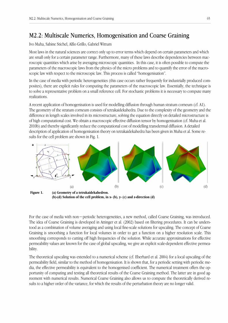
M2.2: Multiscale Numerics, Homogenisation and Coarse GrainingIvo Muha, Sabine Stichel, Alfio Grillo, Gabriel Wittum

Most laws in the natural sciences are correct only up to error terms which depend on certain parameters and whichare small only for a certain parameter range. Furthermore, many of these laws describe dependencies between mac-roscopic quantities which arise by averaging microscopic quantities. In this case, it is often possible to compute theparameters of the macroscopic laws from the physics of the micro problems and to quantify the error of the macro-scopic law with respect to the microscopic law. This process is called “homogenisation”.

In the case of media with periodic heterogeneities (this case occurs rather frequently for industrially produced com-posites), there are explicit rules for computing the parameters of the macroscopic law. Essentially, the technique isto solve a representative problem on a small reference cell. For stochastic problems it is necessary to compute manyrealizations.

A recent application of homogenisation is used for modelling diffusion through human stratum corneum (cf. A1).The geometry of the stratum corneum consists of tetrakaidekahedra. Due to the complexity of the geometry and thedifference in length scales involved in its microstructure, solving the equation directly on detailed microstructure isof high computational cost. We obtain a macroscopic effective diffusion tensor by homogenisation (cf. Muha et al.2010b) and thereby significantly reduce the computational cost of modelling transdermal diffusion. A detaileddescription of application of homogenisation theory on tetrakaidekahedra has been given in Muha et al. Some re-sults for the cell problem are shown in Fig. 1.

For the case of media with non−periodic heterogeneities, a new method, called Coarse Graining, was introduced.The idea of Coarse Graining is developed in Attinger et al. (2002) based on filtering procedures. It can be unders-tood as a combination of volume averaging and using local fine-scale solutions for upscaling. The concept of CoarseGraining is smoothing a function for local volumes in order to get a function on a higher resolution scale. Thissmoothing corresponds to cutting off high frequencies of the solution. While accurate approximations for effectivepermeability values are known for the case of global upscaling, we give an explicit scale-dependent effective permea-bility.

The theoretical upscaling was extended to a numerical scheme (cf. Eberhard et al. 2004) for a local upscaling of thepermeability field, similar to the method of homogenisation. It is shown that, for a periodic setting with periodic me-dia, the effective permeability is equivalent to the homogenised coefficient. The numerical treatment offers the op-portunity of computing and testing all theoretical results of the Coarse Graining method. The latter are in good ag-reement with numerical results. Numerical Coarse Graining also allows us to compute the theoretically derived re-sults to a higher order of the variance, for which the results of the perturbation theory are no longer valid.

(a) (b) (c) (d)

Figure 1. (a) Geometry of a tetrakaidekahedron.(b)-(d) Solution of the cell problem, in x- (b), y- (c) and z-direction (d)

M2.2: Multiscale Numerics, Homogenisation and Coarse Graining 65

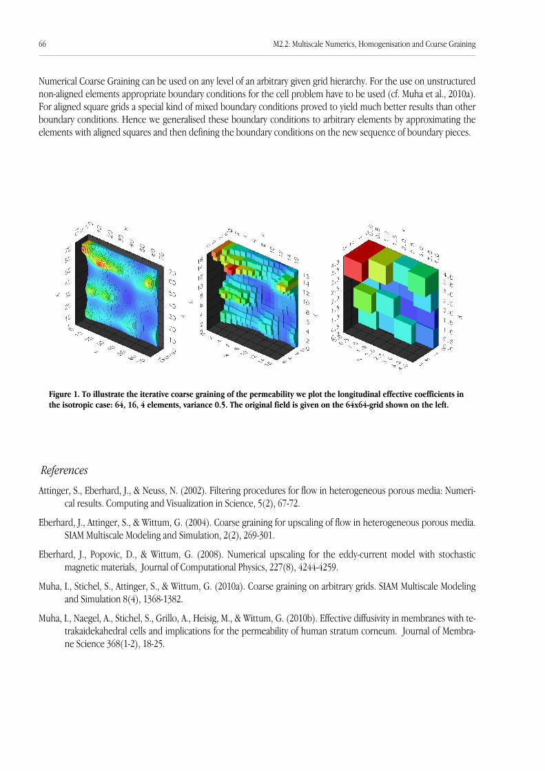
Numerical Coarse Graining can be used on any level of an arbitrary given grid hierarchy. For the use on unstructurednon-aligned elements appropriate boundary conditions for the cell problem have to be used (cf. Muha et al., 2010a).For aligned square grids a special kind of mixed boundary conditions proved to yield much better results than otherboundary conditions. Hence we generalised these boundary conditions to arbitrary elements by approximating theelements with aligned squares and then defining the boundary conditions on the new sequence of boundary pieces.

References

Attinger, S., Eberhard, J., & Neuss, N. (2002). Filtering procedures for flow in heterogeneous porous media: Numeri-cal results. Computing and Visualization in Science, 5(2), 67-72.

Eberhard, J., Attinger, S., & Wittum, G. (2004). Coarse graining for upscaling of flow in heterogeneous porous media.SIAM Multiscale Modeling and Simulation, 2(2), 269-301.

Eberhard, J., Popovic, D., & Wittum, G. (2008). Numerical upscaling for the eddy-current model with stochasticmagnetic materials, Journal of Computational Physics, 227(8), 4244-4259.

Muha, I., Stichel, S., Attinger, S., & Wittum, G. (2010a). Coarse graining on arbitrary grids. SIAM Multiscale Modelingand Simulation 8(4), 1368-1382.

Muha, I., Naegel, A., Stichel, S., Grillo, A., Heisig, M., & Wittum, G. (2010b). Effective diffusivity in membranes with te-trakaidekahedral cells and implications for the permeability of human stratum corneum. Journal of Membra-ne Science 368(1-2), 18-25.

Figure 1. To illustrate the iterative coarse graining of the permeability we plot the longitudinal effective coefficients inthe isotropic case: 64, 16, 4 elements, variance 0.5. The original field is given on the 64x64-grid shown on the left.

66 M2.2: Multiscale Numerics, Homogenisation and Coarse Graining

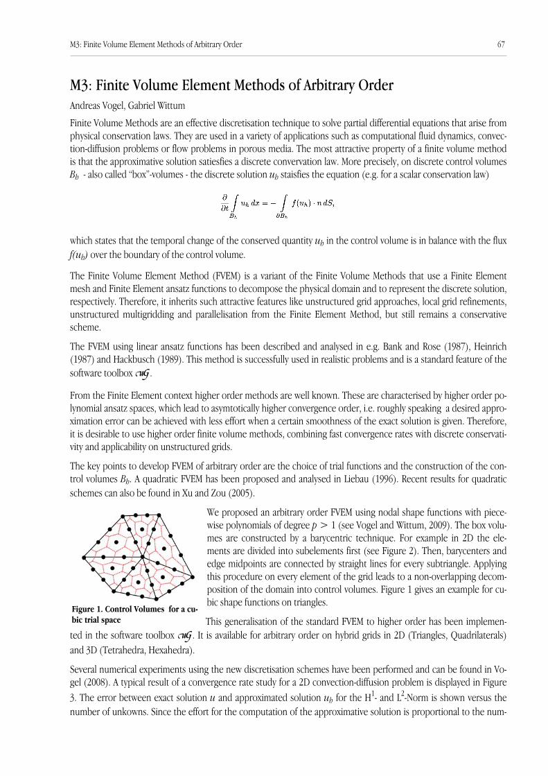
M3: Finite Volume Element Methods of Arbitrary OrderAndreas Vogel, Gabriel Wittum

Finite Volume Methods are an effective discretisation technique to solve partial differential equations that arise fromphysical conservation laws. They are used in a variety of applications such as computational fluid dynamics, convec-tion-diffusion problems or flow problems in porous media. The most attractive property of a finite volume methodis that the approximative solution satiesfies a discrete convervation law. More precisely, on discrete control volumesBh - also called “box”-volumes - the discrete solution uh staisfies the equation (e.g. for a scalar conservation law)

which states that the temporal change of the conserved quantity uh in the control volume is in balance with the fluxf(uh) over the boundary of the control volume.

The Finite Volume Element Method (FVEM) is a variant of the Finite Volume Methods that use a Finite Elementmesh and Finite Element ansatz functions to decompose the physical domain and to represent the discrete solution,respectively. Therefore, it inherits such attractive features like unstructured grid approaches, local grid refinements,unstructured multigridding and parallelisation from the Finite Element Method, but still remains a conservativescheme.

The FVEM using linear ansatz functions has been described and analysed in e.g. Bank and Rose (1987), Heinrich(1987) and Hackbusch (1989). This method is successfully used in realistic problems and is a standard feature of thesoftware toolbox ⋲.

From the Finite Element context higher order methods are well known. These are characterised by higher order po-lynomial ansatz spaces, which lead to asymtotically higher convergence order, i.e. roughly speaking a desired appro-ximation error can be achieved with less effort when a certain smoothness of the exact solution is given. Therefore,it is desirable to use higher order finite volume methods, combining fast convergence rates with discrete conservati-vity and applicability on unstructured grids.

The key points to develop FVEM of arbitrary order are the choice of trial functions and the construction of the con-trol volumes Bh. A quadratic FVEM has been proposed and analysed in Liebau (1996). Recent results for quadraticschemes can also be found in Xu and Zou (2005).

We proposed an arbitrary order FVEM using nodal shape functions with piece-wise polynomials of degree p > 1 (see Vogel and Wittum, 2009). The box volu-mes are constructed by a barycentric technique. For example in 2D the ele-ments are divided into subelements first (see Figure 2). Then, barycenters andedge midpoints are connected by straight lines for every subtriangle. Applyingthis procedure on every element of the grid leads to a non-overlapping decom-position of the domain into control volumes. Figure 1 gives an example for cu-bic shape functions on triangles.

This generalisation of the standard FVEM to higher order has been implemen-ted in the software toolbox ⋲. It is available for arbitrary order on hybrid grids in 2D (Triangles, Quadrilaterals)and 3D (Tetrahedra, Hexahedra).

Several numerical experiments using the new discretisation schemes have been performed and can be found in Vo-gel (2008). A typical result of a convergence rate study for a 2D convection-diffusion problem is displayed in Figure3. The error between exact solution u and approximated solution uh for the H1- and L2-Norm is shown versus thenumber of unkowns. Since the effort for the computation of the approximative solution is proportional to the num-

Figure 1. Control Volumes for a cu-bic trial space

M3: Finite Volume Element Methods of Arbitrary Order 67

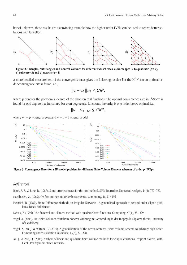
ber of unkowns, these results are a convincing example how the higher order FVEM can be used to achive better so-lutions with less effort.

a) b) c) d)

A more detailed measurement of the convergence rates gives the following results: For the H1-Norm an optimal or-der convergence rate is found, i.e.,

where p denotes the polynomial degree of the choosen trial functions. The optimal convergence rate in L2-Norm isfound for odd degree trial functions. For even degree trial functions, the order is one order below optimal, i.e.

where m = p when p is even and m=p+1 when p is odd.

ReferencesBank, R. E., & Rose, D. (1987). Some error estimates for the box method. SIAM Journal on Numerical Analysis, 24(4), 777–787.

Hackbusch, W. (1989). On first and second order box schemes. Computing, 41, 277-296.

Heinrich, B. (1987). Finite Difference Methods on Irregular Networks - A generalized approach to second order elliptic prob-lems. Basel: Birkhäuser.

Liebau, F. (1996). The finite volume element method with quadratic basis functions. Computing, 57(4), 281-299.

Vogel, A. (2008). Ein Finite-Volumen-Verfahren höherer Ordnung mit Anwendung in der Biophysik. Diploma thesis, Universityof Heidelberg.

Vogel, A., Xu, J. & Wittum, G. (2010). A generalization of the vertex-centered Finite Volume scheme to arbitrary high order.Computing and Visualization in Science, 13(5), 221-228.

Xu, J., & Zou, Q. (2005). Analysis of linear and quadratic finite volume methods for elliptic equations. Preprint AM298, Math.Dept., Pennsylvania State University.

Figure 2. Triangles, Subtriangles and Control Volumes for different FVE schemes: a) linear (p=1), b) quadratic (p=2),c) cubic (p=3) and d) quartic (p=4)

68 M3: Finite Volume Element Methods of Arbitrary Order

1e-07

1e-06

1e-05

0.0001

0.001

0.01

0.1

1

10

1000 10000 100000 1e+06

||u-

u h||H1

Number of Unknowns

FVE1FVE2FVE3FVE4FVE5FVE6FVE7FVE8

1e-09

1e-08

1e-07

1e-06

1e-05

0.0001

0.001

0.01

0.1

1000 10000 100000 1e+06

||u-

u h||L2

Number of Unknowns

FVE1FVE2FVE3FVE4FVE5FVE6FVE7FVE8

Figure 3. Convergence Rates for a 2D model problem for different Finite Volume Element schemes of order p (FVEp)

a) b)

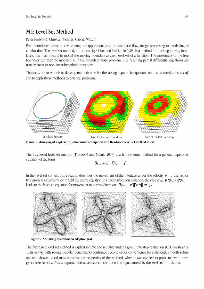
M4: Level Set MethodPeter Frolkovič, Christian Wehner, Gabriel Wittum

Free boundaries occur in a wide range of applications, e.g. in two-phase flow, image processing or modelling ofcombustion. The level-set method, introduced by Osher and Sethian in 1988, is a method for tracking moving inter-faces. The main idea is to model the moving boundary as zero level set of a function. The movement of the freeboundary can then be modeled as initial boundary value problem. The resulting partial differential equations areusually linear or non-linear hyperbolic equations.

The focus of our work is to develop methods to solve the arising hyperbolic equations on unstructured grids in ⋲and to apply these methods to practical problems.

The flux-based level set method (Frolkovič and Mikula 2007) is a finite-volume method for a general hyperbolicequation of the form

In the level set context this equation describes the movement of the interface under the velocity . If the veloci-ty is given as external velocity field the above equation is a linear advection equation, the caseleads to the level set equation for movement in normal direction

The flux-based level set method is explicit in time and is stable under a given time step restriction (CFL constraint).Tests in ⋲ with several popular benchmarks confirmed second order convergence for sufficiently smooth soluti-ons and showed good mass conservation properties of the method, when it was applied to problems with diver-gence-free velocity. This is important because mass conservation is not guaranteed by the level-set formulation.

Level set function Grid for the intial condition Grid at the last time step

M4: Level Set Method 69

Figure 1. Shrinking of a sphere in 3 dimensions computed with flux-based level set method in ⋲

Figure 2. Shrinking quatrefoil on adaptive grid

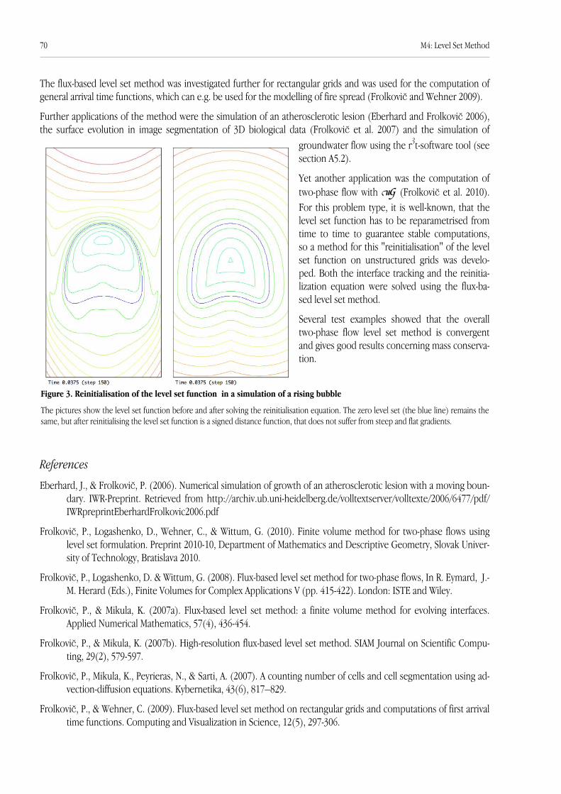
The flux-based level set method was investigated further for rectangular grids and was used for the computation ofgeneral arrival time functions, which can e.g. be used for the modelling of fire spread (Frolkovič and Wehner 2009).

Further applications of the method were the simulation of an atherosclerotic lesion (Eberhard and Frolkovič 2006),the surface evolution in image segmentation of 3D biological data (Frolkovič et al. 2007) and the simulation of

groundwater flow using the r3t-software tool (seesection A5.2).

Yet another application was the computation oftwo-phase flow with ⋲ (Frolkovič et al. 2010).For this problem type, it is well-known, that thelevel set function has to be reparametrised fromtime to time to guarantee stable computations,so a method for this "reinitialisation" of the levelset function on unstructured grids was develo-ped. Both the interface tracking and the reinitia-lization equation were solved using the flux-ba-sed level set method.

Several test examples showed that the overalltwo-phase flow level set method is convergentand gives good results concerning mass conserva-tion.

References

Eberhard, J., & Frolkovič, P. (2006). Numerical simulation of growth of an atherosclerotic lesion with a moving boun-dary. IWR-Preprint. Retrieved from http://archiv.ub.uni-heidelberg.de/volltextserver/volltexte/2006/6477/pdf/IWRpreprintEberhardFrolkovic2006.pdf

Frolkovič, P., Logashenko, D., Wehner, C., & Wittum, G. (2010). Finite volume method for two-phase flows usinglevel set formulation. Preprint 2010-10, Department of Mathematics and Descriptive Geometry, Slovak Univer-sity of Technology, Bratislava 2010.

Frolkovič, P., Logashenko, D. & Wittum, G. (2008). Flux-based level set method for two-phase flows, In R. Eymard, J.-M. Herard (Eds.), Finite Volumes for Complex Applications V (pp. 415-422). London: ISTE and Wiley.

Frolkovič, P., & Mikula, K. (2007a). Flux-based level set method: a finite volume method for evolving interfaces.Applied Numerical Mathematics, 57(4), 436-454.

Frolkovič, P., & Mikula, K. (2007b). High-resolution flux-based level set method. SIAM Journal on Scientific Compu-ting, 29(2), 579-597.

Frolkovič, P., Mikula, K., Peyrieras, N., & Sarti, A. (2007). A counting number of cells and cell segmentation using ad-vection-diffusion equations. Kybernetika, 43(6), 817–829.

Frolkovič, P., & Wehner, C. (2009). Flux-based level set method on rectangular grids and computations of first arrivaltime functions. Computing and Visualization in Science, 12(5), 297-306.

70 M4: Level Set Method

Figure 3. Reinitialisation of the level set function in a simulation of a rising bubble

The pictures show the level set function before and after solving the reinitialisation equation. The zero level set (the blue line) remains thesame, but after reinitialising the level set function is a signed distance function, that does not suffer from steep and flat gradients.

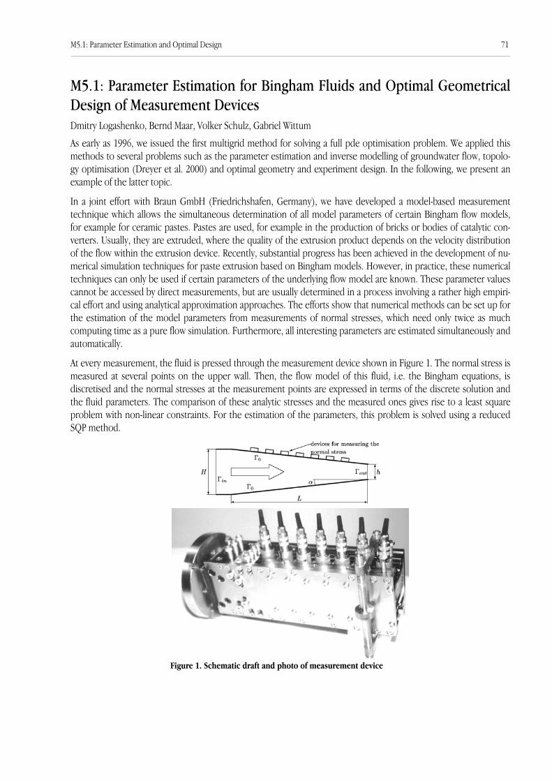
M5.1: Parameter Estimation for Bingham Fluids and Optimal GeometricalDesign of Measurement DevicesDmitry Logashenko, Bernd Maar, Volker Schulz, Gabriel Wittum

As early as 1996, we issued the first multigrid method for solving a full pde optimisation problem. We applied thismethods to several problems such as the parameter estimation and inverse modelling of groundwater flow, topolo-gy optimisation (Dreyer et al. 2000) and optimal geometry and experiment design. In the following, we present anexample of the latter topic.

In a joint effort with Braun GmbH (Friedrichshafen, Germany), we have developed a model-based measurementtechnique which allows the simultaneous determination of all model parameters of certain Bingham flow models,for example for ceramic pastes. Pastes are used, for example in the production of bricks or bodies of catalytic con-verters. Usually, they are extruded, where the quality of the extrusion product depends on the velocity distributionof the flow within the extrusion device. Recently, substantial progress has been achieved in the development of nu-merical simulation techniques for paste extrusion based on Bingham models. However, in practice, these numericaltechniques can only be used if certain parameters of the underlying flow model are known. These parameter valuescannot be accessed by direct measurements, but are usually determined in a process involving a rather high empiri-cal effort and using analytical approximation approaches. The efforts show that numerical methods can be set up forthe estimation of the model parameters from measurements of normal stresses, which need only twice as muchcomputing time as a pure flow simulation. Furthermore, all interesting parameters are estimated simultaneously andautomatically.

At every measurement, the fluid is pressed through the measurement device shown in Figure 1. The normal stress ismeasured at several points on the upper wall. Then, the flow model of this fluid, i.e. the Bingham equations, isdiscretised and the normal stresses at the measurement points are expressed in terms of the discrete solution andthe fluid parameters. The comparison of these analytic stresses and the measured ones gives rise to a least squareproblem with non-linear constraints. For the estimation of the parameters, this problem is solved using a reducedSQP method.

M5.1: Parameter Estimation and Optimal Design 71

Figure 1. Schematic draft and photo of measurement device

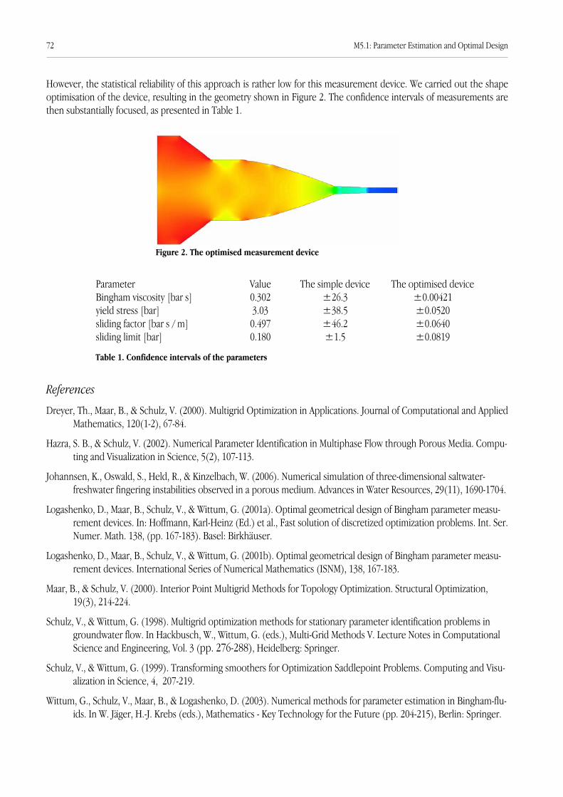
However, the statistical reliability of this approach is rather low for this measurement device. We carried out the shapeoptimisation of the device, resulting in the geometry shown in Figure 2. The confidence intervals of measurements arethen substantially focused, as presented in Table 1.

References

Dreyer, Th., Maar, B., & Schulz, V. (2000). Multigrid Optimization in Applications. Journal of Computational and AppliedMathematics, 120(1-2), 67-84.

Hazra, S. B., & Schulz, V. (2002). Numerical Parameter Identification in Multiphase Flow through Porous Media. Compu-ting and Visualization in Science, 5(2), 107-113.

Johannsen, K., Oswald, S., Held, R., & Kinzelbach, W. (2006). Numerical simulation of three-dimensional saltwater-freshwater fingering instabilities observed in a porous medium. Advances in Water Resources, 29(11), 1690-1704.

Logashenko, D., Maar, B., Schulz, V., & Wittum, G. (2001a). Optimal geometrical design of Bingham parameter measu-rement devices. In: Hoffmann, Karl-Heinz (Ed.) et al., Fast solution of discretized optimization problems. Int. Ser.Numer. Math. 138, (pp. 167-183). Basel: Birkhäuser.

Logashenko, D., Maar, B., Schulz, V., & Wittum, G. (2001b). Optimal geometrical design of Bingham parameter measu-rement devices. International Series of Numerical Mathematics (ISNM), 138, 167-183.

Maar, B., & Schulz, V. (2000). Interior Point Multigrid Methods for Topology Optimization. Structural Optimization,19(3), 214-224.

Schulz, V., & Wittum, G. (1998). Multigrid optimization methods for stationary parameter identification problems ingroundwater flow. In Hackbusch, W., Wittum, G. (eds.), Multi-Grid Methods V. Lecture Notes in ComputationalScience and Engineering, Vol. 3 (pp. 276-288), Heidelberg: Springer.

Schulz, V., & Wittum, G. (1999). Transforming smoothers for Optimization Saddlepoint Problems. Computing and Visu-alization in Science, 4, 207-219.

Wittum, G., Schulz, V., Maar, B., & Logashenko, D. (2003). Numerical methods for parameter estimation in Bingham-flu-ids. In W. Jäger, H.-J. Krebs (eds.), Mathematics - Key Technology for the Future (pp. 204-215), Berlin: Springer.

72 M5.1: Parameter Estimation and Optimal Design

Figure 2. The optimised measurement device

Table 1. Confidence intervals of the parameters

ParameterBingham viscosity [bar s]yield stress [bar]

Value The simple device0.3023.03

±26.3±38.5

sliding factor [bar s / m]sliding limit [bar]

0.4970.180

±46.2±1.5

The optimised device±0.00421±0.0520±0.0640±0.0819

M5.2: Parameter Estimation for Calcium SignallingGillian Queisser, Gabriel Wittum

A recurring challenge in neurobiology is finding experimental methods to access biological parameters within celltissue or single cells. Measuring diffusion properties of molecules in vivo or in vitro, opposed to an artificialexperimental setting, poses difficulties since these parameters are only indirectly accessible. Literature on diffusionproperties of cellular and nuclear calcium is sparse. Until now only one publication touching on that topic is knownto us (Allbritton et al. 1992). Furthermore, in Allbritton et al. (1992) experiments are not carried out in vitro, but inan artificial setting using cytosolic-like media.

In other neuroscience projects of the G-CSC, calcium diffusion properties are part of underlying mathematicalmodels. We therefore saw the need to quantify calcium diffusion by developing inverse modelling tools, based onexperimental data. A prerequisite for developing an adequate parameter estimation method, is to know what kind ofdata is recordable experimentally. A method for investigating the diffusion barrier properties of the nuclearmembrane was published by the Bading lab at the IZN in Heidelberg (Eder and Bading 2007). Laser-assisted calciumuncaging methods allow controlled release of calcium in the cell, and the spatio-temporal development of thiscalcium signal can be recorded. For the schematics of this method see Figure 1.

This data can be used to estimate the diffusion coefficient of cellular calcium (nuclear or cytosolic). As an objectivefunction for the optimisation problem we define

where D denotes the diffusion coefficient of nuclear calcium, which is to be estimated, c the experimental data inspace and time (i and j resp.) and u the model data resp. to D. Finding an optimal model fit for the experimentaldata means minimising the objective function F. Local approximation and minimisation of the objective functionyields a linearised quadratic function of the form

source

1.33µm

2.66µm

...

etc.

nucleus

cytoplasm

field of view / scanning area

Figure 1. Left: Set up of the laser-assisted calcium uncaging experiments. Calcium can be locally released by a UV-laser, either in thenucleus or in the cytosol of single cells. Right: Measuring spatio-temporal calcium patterns; a linear recording band is defined, averagingdata vertically (accounting for experimental variability) and measuring at discrete point in horizontal direction.

M5.2: Parameter Estimation for Calcium Signalling 73

with

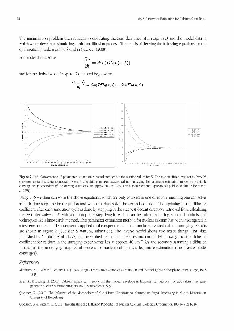
The minimisation problem then reduces to calculating the zero derivative of u resp. to D and the model data u,which we retrieve from simulating a calcium diffusion process. The details of deriving the following equations for ouroptimisation problem can be found in Queisser (2008):

For model data u solve

and for the derivative of F resp. to D (denoted by g), solve

Using uG we then can solve the above equations, which are only coupled in one direction, meaning one can solve,in each time step, the first equation and with that data solve the second equation. The updating of the diffusioncoefficient after each simulation cycle is done by stepping in the steepest decent direction, retrieved from calculatingthe zero derivative of F with an appropriate step length, which can be calculated using standard optimisationtechniques like a line-search method. This parameter estimation method for nuclear calcium has been investigated ina test environment and subsequently applied to the experimental data from laser-assisted calcium uncaging. Resultsare shown in Figure 2 (Queisser & Wittum, submitted). The inverse model shows two major things. First, datapublished by Albritton et al. (1992) can be verified by this parameter estimation model, showing that the diffusioncoefficient for calcium in the uncaging experiments lies at approx. 40 um^2/s and secondly assuming a diffusionprocess as the underlying biophysical process for nuclear calcium is a legitimate estimation (the inverse modelconverges).

ReferencesAllbritton, N.L., Meyer, T., & Stryer, L. (1992). Range of Messenger Action of Calcium Ion and Inositol 1,4,5-Triphosphate. Science, 258, 1812-

1815.

Eder, A., & Bading, H. (2007). Calcium signals can freely cross the nuclear envelope in hippocampal neurons: somatic calcium increasesgenerate nuclear calcium transients. BMC Neuroscience, 8, 57.

Queisser, G., (2008). The Influence of the Morphology of Nuclei from Hippocampal Neurons on Signal Processing in Nuclei. Dissertation,University of Heidelberg.

Queisser, G. & Wittum, G. (2011). Investigating the Diffusion Properties of Nuclear Calcium. Biological Cybernetics, 105(3-4), 211-216.

0

20

40

60

80

100

120

140

160

1 2 3 4 5 6 7 8 9 10 11 12 13 14 15 16 17 18 19 20 21 22 23 24 25 26No . o f I t e ra t i ons

Dif

fusi

on C

oeff

icie

nt

D_0 = 1.0D_0 = 20.0D_0 = 50.0D_0 = 100.0D_0 = 150.0

Figure 2. Left: Convergence of parameter estimation runs independent of the starting values for D. The test coefficient was set to D=100,convergence to this value is quadratic. Right: Using data from laser-assisted calcium uncaging the parameter estimation model shows stableconvergence independent of the starting value for D to approx. 40 um^2/s. This is in agreement to previously published data (Allbritton etal. 1992).

74 M5.2: Parameter Estimation for Calcium Signalling

M8, M9, T7: Geometry Modelling and Grid GenerationDirk Feuchter, Alexander Fuchs, Andreas Hauser, Sebastian Reiter, Martin Stepniewski, Gabriel Wittum

Many physical processes occur in rather complex domains. For simulating phenomena with practical relevance,mapping these domains onto a computational domain and triangulating them can only be carried out with powerfuland specialised tools. In order to cope with the specific properties of the problems that are treated in numerical si-mulations, different approaches are required to preserve the special characteristics of the associated geometries du-ring discretisation.

First, a rather general way of utilising arbitrary CAD geometries is pre-sented, while the second approach is adopted for highly anisotropicdomains occurring in simulating groundwater flow or transdermal diffu-sion of xenobiotics into the epidermis. A third approach allows the fullyautomated generation of tetrahedral grids from arbitrary piecewise line-ar surface geometries. All approaches produce grids ready for simulati-on with ⋲.

Finally a new approach to successive multigrid refinement is described.The required preprocessing for this technique is currently being in-tegrated into our toolchain.

CAD Geometries

In many industrial applications, the starting point for a numerical simu-lation is the modelling and discretisation of CAD geometries. To modelcomplex geometries, the 3D-modeller ProE is applied. This also enablesthe import of neutral files via IGES and STEP interfaces which in turn al-lows geometries generated by other software on different platforms tobe considered. Then, a very fine surface mesh is generated in ProE thatnow acts as the new approximated domain, which is either importedinto ⋲ or into the powerful mesh generator ICEMCFD. This grid gen-erator tool is able to triangulate complex geometries, resulting in a vol-ume mesh with far more than 10 million elements that is finally im-ported into ⋲ via a linear domain interface. The data transfer betweenthe several tools is realised by Perl converters and depicted in the figureon the left-hand side.

Three examples of real-world geometries are presented in Figure 1, 2and 3. Electromagnetics and heat transfer are simulated using thesegeometries. The first figure gives insight into a module of a static mixer.Figure 2 represents a part of an electrical device with lamellae for cool-ing, while the last figure shows a gas-isolated switch gear. The numberof volume elements varies from 5,000 to 100,000 elements on the coarsegrid and from 200,000 up to and more than 64 million on the finest gridthat approximates the very fine surface mesh sufficiently and thus theoriginal geometry.

M8: Geometry Modelling and Grid Generation 75

Figure 1. Path from CAD-tool (ProE) to ⋲

Geometry and grid generation for anisotropically layered domains

Solving partial differential equations in geoscientific applications (e.g. density-driven flow) or in pharmaceutical appli-cations (e.g. transdermal diffusion of xenobiotics into the epidermis (stratum corneum)) implies a complex prepro-cessing for geometry modelling and grid generation. Geoscientific domains are often assemblies of layers with a di-mension of many kilometres in the horizontal direction, but a dimension of only some metres in the vertical direc-tion. This yields the typical strong anisotropy. Further geological characteristics possibly occur: layers crop out, so-metimes contain lenses or fractures, display overhangs (e.g. salt domes) or faults. Layered domains of cells such asthe stratum corneum consist of many corneocytes which are approx. 30 µm wide and 1 µm in height and are sur-rounded by a homogeneous lipid layer of 0.1 µm. Simulations of such anisotropically layered domains require gridswith suitable sizes and shapes of the elements. We develop methods for geometry and grid generation using the fileformats “lgm” and “ng” used in our numerical simulation system ⋲ to describe complex geometries and grids.First, with vertical lines and a protrusion technique, LD_Modeller2.5D creates geometries and grids consisting of tri-angles, quadrilaterals in 2D and prisms and hexahedra in 3D, suitable for a certain kind of geoscientific “L”ayered“D”omain.

In a second approach, we model more complicated layered domains, using the gridding methods of surfer or any data inter-polation software which is able to describe a separating surface between two layers based on geological input data(e.g. borehole data). With a thickness approach, LD_Modeller3D can include domains with geological characteristics(as above), leading to a consistent assembly of all layers available to the 3D simulation process with ⋲. In a secondstep, the grid generator of LD_Modeller3D creates hybrid meshes consisting of pyramids, tetrahedra, prisms andmainly hexahedra. Using vertical lines during the grid generation leads to good element angles.

76 M8: Geometry Modelling and Grid Generation

Figure 2. Medium voltage switch (ABB) Figure 3. Gas-insulated switching gear: full configuration

Figure 4. The WIPP domain, a typical highly anisotropic domain from hydrogeology

In case of anisotropically layered domains such as the epidermis, Cuboid_Modeller describes each corneocyte as acuboid. The corneocytes and the lipid layers are both meshed uniquely with hexahedra. In a second approach, weuse nested tetrakaidekahedra, describing a corneocyte in the lipid layer. Tetrakaidekahedra are suitable becausethey overlap, and it is possible to create a dense packing of 100%. Tkd_Modeller creates a geometry file in the lgm-format and a hybrid grid consisting of hexahedra, prisms, pyramids and tetrahedra in the ng-format.

Additionally, we developed the grid generator ARTE, based on ART (Almost Regular Tetrahedra). ARTE keeps to in-terior faces and is able to expand prescribed internal faces to thin layers and to generate prisms for anisotropic lay-ers. Special algorithms are developed for treating intersecting faces.

Figure 5.A 3d grid of Norderney, an East-Frisianisland in the North Sea. The grid consis-ting of hexahedra, prisms, pyramidsand tetrahedra is generated by Ld_Mod-eller3d and follows the geometry.

M8: Geometry Modelling and Grid Generation 77

Figure 6. Geometry and grid of two different 3D models for human stratum corneum. On the left the corneocytes aremodelled by cuboids, on the right by tetrakaidekhedra.

Figure 7. Thin layer grids generated by ARTEFrom left to right: Grid of the Norderney domain. The next three images show the expansion of intersecting interior fa-ces to thin layers with special treatment of layer intersections.

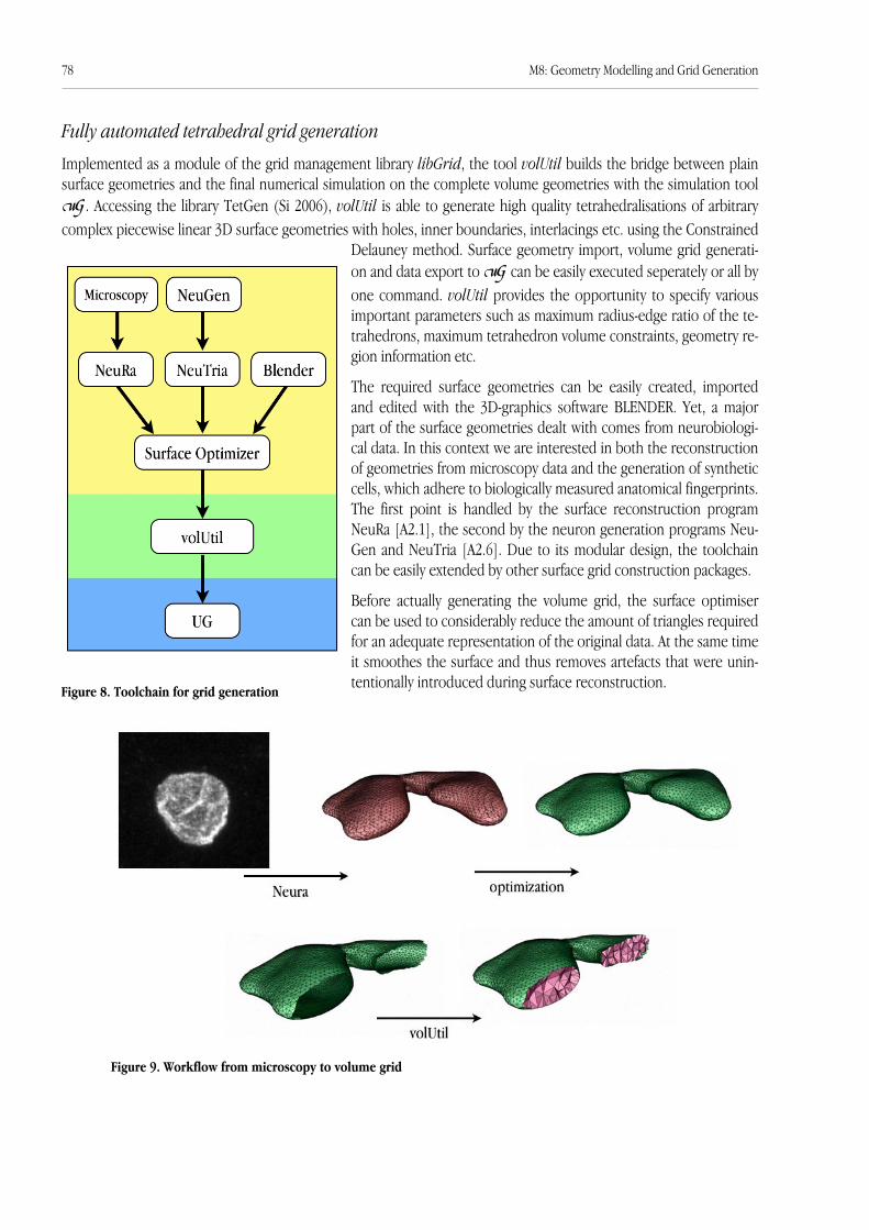
Fully automated tetrahedral grid generation

Implemented as a module of the grid management library libGrid, the tool volUtil builds the bridge between plainsurface geometries and the final numerical simulation on the complete volume geometries with the simulation tool⋲. Accessing the library TetGen (Si 2006), volUtil is able to generate high quality tetrahedralisations of arbitrarycomplex piecewise linear 3D surface geometries with holes, inner boundaries, interlacings etc. using the Constrained

Delauney method. Surface geometry import, volume grid generati-on and data export to ⋲ can be easily executed seperately or all byone command. volUtil provides the opportunity to specify variousimportant parameters such as maximum radius-edge ratio of the te-trahedrons, maximum tetrahedron volume constraints, geometry re-gion information etc.

The required surface geometries can be easily created, importedand edited with the 3D-graphics software BLENDER. Yet, a majorpart of the surface geometries dealt with comes from neurobiologi-cal data. In this context we are interested in both the reconstructionof geometries from microscopy data and the generation of syntheticcells, which adhere to biologically measured anatomical fingerprints.The first point is handled by the surface reconstruction programNeuRa [A2.1], the second by the neuron generation programs Neu-Gen and NeuTria [A2.6]. Due to its modular design, the toolchaincan be easily extended by other surface grid construction packages.

Before actually generating the volume grid, the surface optimisercan be used to considerably reduce the amount of triangles requiredfor an adequate representation of the original data. At the same timeit smoothes the surface and thus removes artefacts that were unin-tentionally introduced during surface reconstruction.

78 M8: Geometry Modelling and Grid Generation

Figure 9. Workflow from microscopy to volume grid

Figure 8. Toolchain for grid generation

Subdivision Surface Refinement

Subdivision Surface Refinement is a technique to describe either interpolating or approximating 2D smooth surfa-ces, which result as the limit of the successive refinement of a piecewise linear control mesh and (re-)positioning ofits vertices. Vertices of the refined mesh are positioned using weighted averages of the vertices of the unrefinedmesh. With Loop's scheme (Loop 1987), which is based on B-Spline approximation, the limit surface is ensured tobe two times continuously differentiable everywhere except for irregular vertices, where the surface is only one timecontinuously differentiable. Furthermore, this method can be applied to regular 2D geometries of arbitrary topolo-gy.

Multigrid methods require successive refinement. The classical approach is based on a geometrical projection, whe-re the refined mesh is projected onto a separate boundary description. This method is prone to error and likely tocause problems on geometries with inversions, which occur quite often in neurobiological data. In this case subdivi-sion refinement represents a promising alternative. After an initial surface-fitting step, which can be done during sur-face-optimisation, successive Subdivision Refinement automatically leads to a grid whose boundary approximatesthe surface geometry of the original data. While this technique is not intended to replace the classical refinementmethods, it is a stable, robust and fast alternative, perfectly suited for geometries based on neurobiological data.

M8: Geometry Modelling and Grid Generation 79

Figure 10. Workflow from NeuGen to volume grid

Figure 11. Successive subdivision refinement steps and limit surface (from Zorin et al. 2000)

Figure 12. Subdivision Refinement applied on a nucleus during simulation with ⋲

References

Feuchter, D., Stemmermann, U., & Wittum, G. (2001). Description and Generation of Geometries and Grids for Laye-red Domains. 17th GAMM Seminar on Construction of Grid Generation Algorithms, ISBN 3-00-007753-7. Re-trieved from http://www.mis.mpg.de/conferences/gamm/2001/GAMM_2001_Abstracts_7.html

Feuchter, D., Heisig, M., & Wittum, G. (2006). A geometry model for the simulation of drug diffusion through stra-tum corneum. Computing and Visualization in Science, 9(2), 117-130.

Fuchs, A., & Wittum, G. (2003). Grid Generation for Domains with Thin Layers. WiR-Preprint, 02/03, Heidelberg.

Loop, C. (1987). Smooth Subdivision Surfaces Based on Triangles. M.S. Mathematics thesis, University of Utah, USA.

Si, H. (2006). TetGen - A Quality Tetrahedral Mesh Generator and Three-Dimensional Delauney Triangulator, User'sManual. Retrieved from http://tetgen.berlios.de/

Zorin, D., DeRose, T., Levin, A., Schröder, P., Kobbelt, L., & Sweldens, W. (2000). Subdivision for Modeling and Ani-mation. SIGGRAPH 2000 Coursenotes. Retrieved from: http://www.cs.rutgers.edu/~decarlo/readings/subdiv-sg00c.pdf

80 M8: Geometry Modelling and Grid Generation

T4: Visualisation: VRL/UG InterfaceMichael Hoffer, Christian Poliwoda, Gabriel Wittum

VRL is a flexible library for automatic and interactive object visualisation on the Java platform. It provides a visualprogramming interface including meta programming support and tools for real−time 3D graphic visualisation.

Mapping programme functionality to graphical interfaces is traditionally a manual and work−intensive process. VRLtries to simplify the creation of user interfaces by using a declarative approach. Instead of giving specific instructionson how to generate the user interface it is only necessary to define the functionality of the user interface. VRL analy-ses the functionality provided by the Java objects that shall be visualised and uses three types of visual components

to create a graphical user interface that reflects thefunctionality provided by the object: object visuali-sations, method visualisations and parameter visua-lisations (see Figure 1). Parameter visualisations arethe most individual part of the VRL GUI generation.Therefore VRL provides a plugin interface that al-lows to add custom visualisations. This includes in-teractive 2D and 3D visualisations. In addition tothe automatic visualisation, it is possible to specifydata dependencies. This is necessary to define com-plex workflows. All connections are type safe. It ispossible to define custom contracts for data validati-

on. The messaging system notifies the user about incorrect input. VRL can also execute external tools, i.e., performtasks that are usually performed on the command line. Thus, it is able to integrate external tools for defining a prob-lem specific workflow which consists of several independent tools. Although not limited to a specific domain, VRLcomponents are optimised for technical simulation. Figure 2 shows an example visualisation:

To define method calls independently from data dependencies, VRL enables the definition of a linear control flow(see Figure 3). With this additional information it is possible to compile a VRL workflow as Java class with one me-

thod. Instances of this class can be visualised like any other Java object. Another important aspect is the usage of thevisually formulated functionality by any other Java based software. This includes non−graphical applications.

Figure 1. VRL component types

Figure 2. Visualisation of a simple Java object

T4: Visualisation: VRL/UG Interface 81

Figure 3. Visualisation of the control flow

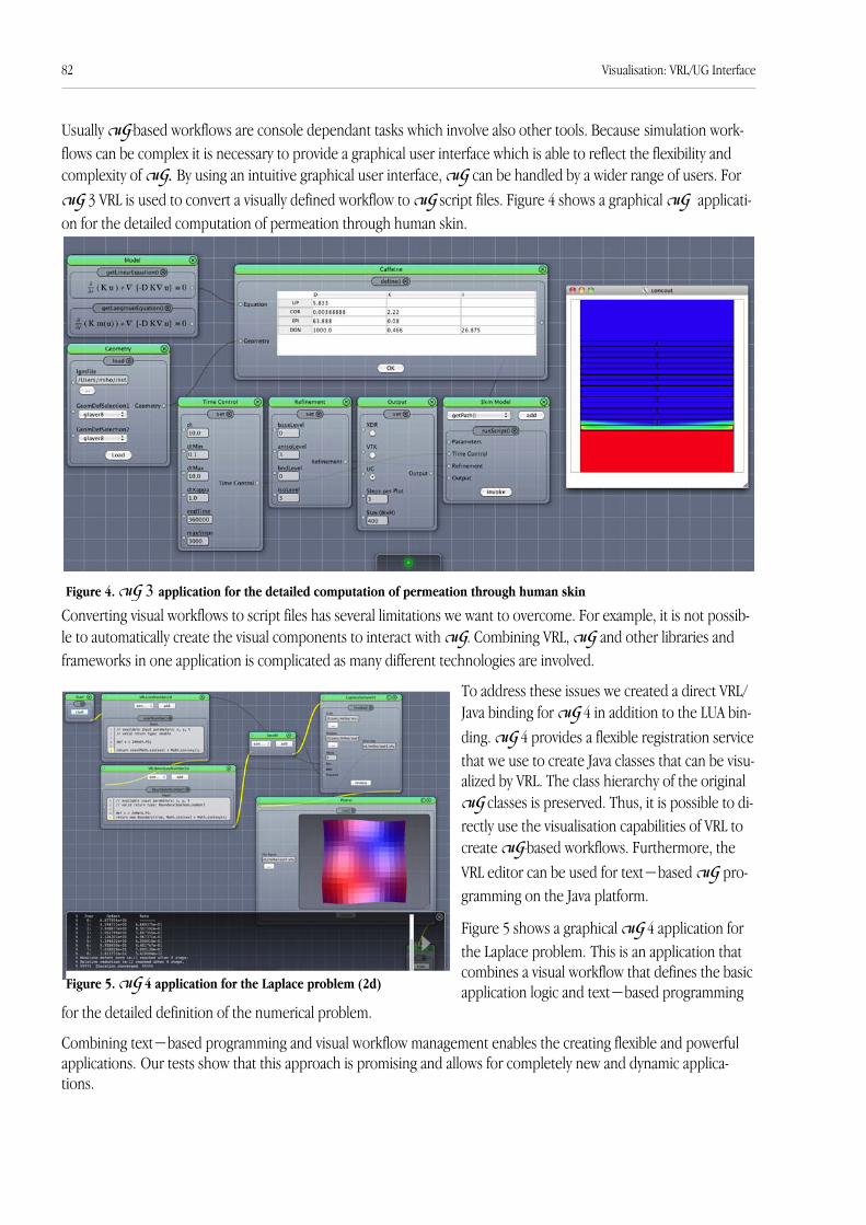
Usually uG­based workflows are console dependant tasks which involve also other tools. Because simulation work-flows can be complex it is necessary to provide a graphical user interface which is able to reflect the flexibility andcomplexity of uG. By using an intuitive graphical user interface, uG can be handled by a wider range of users. ForuG 3 VRL is used to convert a visually defined workflow to uG script files. Figure 4 shows a graphical uG applicati-on for the detailed computation of permeation through human skin.

Converting visual workflows to script files has several limitations we want to overcome. For example, it is not possib-le to automatically create the visual components to interact with uG. Combining VRL, uG and other libraries andframeworks in one application is complicated as many different technologies are involved.

To address these issues we created a direct VRL/Java binding for uG 4 in addition to the LUA bin-ding. uG 4 provides a flexible registration servicethat we use to create Java classes that can be visu-alized by VRL. The class hierarchy of the originaluG classes is preserved. Thus, it is possible to di-rectly use the visualisation capabilities of VRL tocreate uG­based workflows. Furthermore, theVRL editor can be used for text−based uG pro-gramming on the Java platform.

Figure 5 shows a graphical uG 4 application forthe Laplace problem. This is an application thatcombines a visual workflow that defines the basicapplication logic and text−based programming

for the detailed definition of the numerical problem.

Combining text−based programming and visual workflow management enables the creating flexible and powerfulapplications. Our tests show that this approach is promising and allows for completely new and dynamic applica-tions.

Figure 4. uG 3 application for the detailed computation of permeation through human skin

Figure 5. uG 4 application for the Laplace problem (2d)

82 Visualisation: VRL/UG Interface

T5: Simulation Software Library SGDmitry Logashenko, Gabriel Wittum

As a counterpart of ⋲, we developed the library SG (structured grids). This is an efficient tool for computations ontopologically rectangular grids of arbitrary dimension. It profits from the special data structures for the representa-tion of these grids. Furthermore, for efficient simulations of high-dimensional problems, it supports the combina-tion technique for sparse grids (Zenger, 1990). The current version of the library (SG2) is capable of handling a widerange of discretisations of systems of PDEs on structured grids, including e.g. time-dependent non-linear problemson staggered grids, and contains efficient numerical solvers, e.g. multigrid methods. It provides a flexible object-ori-ented programming interface for numerical methods with the possibility of reading method-specific parametersfrom initialisation files. The combination technique is parallelised on the base of the MPI library. SG is implementedin C++ programming language and is platform independent.

The main field of the applications of SG are high-dimensional problems. In the combination technique for thesparse grids, the system of the PDEs is discretised and solved independently on several grids obtained from the

same coarse grid by anisotropic refinement. Figure 1 demon-strates this method in 2 dimensions. The numerical solutionon the sparse grid is a linear combination of the numericalsolutions on the red and the blue regular grids, which arecomputed independently of each other. The accuracy of thissolution is approximately equivalent to that of the solutionon the full regular grid with stepsize h, provided the solutionis sufficently smooth. But in high-dimensional cases, thenumber of degrees of freedom on all the grids involved in thecombination technique is essentially smaller then for the fullregular grid with the same grid step. Furthermore, the com-putations of the solutions on the regular grids in the combi-nation technique can be performed on different processorswithout communication. This allows very efficientparallelisation of the computations. This approach was usedfor high dimensional problems in the computational finance(see Section A3).

Figure 1. Combination technique for the sparse grids

Figure 2. Simulation of biological cell growth with SG2

T5: Simulation Software Library SG 83

h

nu

trie

nt

sto

rag

e

cell size0.1 1

1

0

nu

trie

nt

sto

rag

e

cell size0.1 1

1

0

nu

trie

nt

sto

rag

e

cell size0.1 1

1

0

t = 0, c = 5 t = 0.25, c = 4.52 t = 25, c = 0.33

We also applied this approach for simulations of population dynamics. Figure 2 presents results of a simulation of thebiological cell growth in a stirred tank. The medium containing the cells (e.g. bacteria) and the nutrient is consideredto be well mixed so that it is homogenious. The nutrient is described by its concentration c in the medium. The cellsconsume the nutrient and store it in their internal nutrient storage. Furthermore, they convert this nutrient tobiomass characterised by cell size. The whole cell population is therefore described by the number density functioncharacterising the distribution of the cells in coordinate system “cell size × stored nutrient” (these values arescaled). The model describing these processes is a system of an integro- partial differential equation for the numberdensity function and an ordinary differential equation with an integral term for the concentration c (see Fischer et al.2006) in the coordinates space, time, cell size and stored nutrient. This system is solved using the combination tech-nique for the sparce grids which allows also efficient treatment of the integral terms. More complicated biologicalmodels involving more parameters for the description of the population can be handled in the same way.

SG2 can be also used for efficient computations on regular structured (non-sparse) grids. Figure 3 presents a simula-tion of the Navier-Stokes flow coupled with the transport in a stirred tank. In this example, the discretisation of theNavier-Stokes equations is based on staggered grids.

Further applications include image processing. The possibility to link SG2 as an external library to other software wasused in Mang et al. 2009 for a method tracking fibers in the brain. In this application, the SG2 solvers were used tosimulate the self-diffusion in small areas of the brain to determine the direction of the fibers and showed very goodperformance.

References

Fischer, T., Logashenko, D., Kirkilionis, M., & Wittum, G. (2006). Fast Numerical Integration for Simulation ofStructured Population Equations. Mathematical Models and Methods in Applied Sciences, 16(12), 1987-2012.

Mang, S. C., Logashenko, D., Gembris, D., Wittum, G., Grodd, W., & Klose, U. (2010). Diffusion Simulation BasedFiber Tracking using Time-of-Arrival Maps. Magnetic Resonance Materials in Physics, Biology and Medicine,23(5-6), 391-398.

Zenger, C. (1990): Sparse Grids. SFB-Bericht 342/18/90, Lehrstuhl für Informatik V, TU München.

Figure 3: Simulation of flow andtransport in a stirred tank with SG

84 T5: Simulation Software Library SG

T8: NeuGen: A Tool for the Generation of Realistic Morphology of Corti-cal Neurons and Neural Networks in 3DJens Eberhard, Alexander Wanner, Sergei Wolf, Gillian Queisser, Gabriel Wittum

NeuGen (Eberhard et al. 2006) is a tool for the efficient generation and description of dendritic and axonal morpho-logy of realistic neurons and neural networks in 3D. It is based on experimental data. The ‘in silico’ neurons are ba-sed on cells of cortical columns in the neocortex. The software is available at http://www.neugen.org

The idea for the development of NeuGen has been to be able to simulate networks of synaptically connected neu-rons in a cortical column. The NeuGen project is mainly a result of the fact that experimental data is available nowa-days to extract the anatomical fingerprints of the cells and to generate synthetic neuron geometries.

NeuGen is an on-going software project which will be extended by additional features. A graphical user interface isincluded in the newest NeuGen version which makes program control and assignment of values to the configurationparameters very easy. In recent developments, we began developing a neuroanatomical model of the hippocampus.New classes of neurons, e.g. granule cells, CA1 pyramidal cells and CA3 pyramidal cells and different types ofinterneurons have been implemented.

References

Wolf, S., Grein, S., & Queisser, G. (2011). Employing NeuGen 2.0 to automatically generate realistic morphologies ofhippocampal neurons and neural networks in 3D. Manuscript submitted for publication.

Eberhard, J. P., Wanner, A., & Wittum, G. (2006). NeuGen: A tool for the generation of realistic morphology of corti-cal neurons and neural networks in 3D. Journal of Neurocomputing, 70(1-3), 327-342.

NeuGen: http://www.neugen.org

T8: NeuGen 85

Figure 1. From left: L2/3 pyramidal cell, L4 spiny stellate cell, L5A pyramidal neuron, L5B pyramidal neuron , L4 starpyra-midal cell, network with 100 cells

T9: NeuTria: A Tool for the Triangulation of Realistic Morphologies ofCortical Neurons and Neural Networks in 3DNiklas Antes, Sebastian Reiter, Gillian Queisser, Gabriel Wittum

NeuTria is a software tool for generating closed 3-d surface grids from abstract spatial information. One example isthe generation of neurons and networks from abstract dataprovided by NeuGen.

In NeuGen (Eberhard et al. 2006) the geometry is composedof frustums, see Figure 1 (right). For detailed 3-d models ofcellular and sub-cellular signal processing we need a closedsurface of the neurons, whereas the list of frustums does notdefine closed surfaces.

NeuTria is a software tool to generate an approximation ofthe given “raw data” and calculates closed surfaces – compo-sed of triangles – from NeuGen-generated files. It also createsa geometry of synapses, which in NeuGen only is provided aselectrophysical data. Because the lists of frustums describinga dendrite or an axon are too angular, the program also gene-rates a smoothed graph along a dendrite. Very difficult is thegeneration of correct geometries at intersections and soma.

References

Antes, N. (2009): Ein Werkzeug zur Erzeugung von Oberflächengeometrien von Neuronen. Staatsexamensarbeit, Fa-kultät Mathematik, Universität Heidelberg.

Eberhard, J. P., Wanner, A., & Wittum, G. (2006). NeuGen: A tool for the generation of realistic morphology of corti-cal neurons and neural networks in 3D. Neurocomputing, 70(1-3), 327-342.

Figure 1. The geometry of dendritic branches is representedas a sequence of frustums. The sections are devided intocompartments.

86 T9: NeuTria

Figure 2.Left: A generated network fora cortical column with 20cells.Right top: A dendriticbranching point. A synapse(middle) and soma (right).

CF1: Asset/Liability Management in InsuranceThomas Gerstner

Much effort has been spent on the development of stochastic asset-liability management (ALM) models for lifeinsurance companies in the last years. Such models are becoming more and more important due to newaccountancy standards, greater globalisation,stronger competition, more volatile capitalmarkets and long periods of low interest rates.They are employed to simulate the medium andlong-term development of all assets and liabilities.This way, the exposure of the insurance companyto financial, mortality and surrender risks can beanalysed. The results are used to supportmanagement decisions regarding, e.g., the assetallocation, the bonus declaration or thedevelopment of more profitable and competitiveinsurance products. The models are also appliedto obtain market-based, fair value accountancystandards as required by Solvency II and theInternational Financial Reporting Standard.

Due to the wide range of path-dependencies, guarantees and option-like features of insurance products, closed-form representations of statistical target figures, like expected values or variances, which in turn yield embeddedvalues or risk-return profiles of the company, are in general not available. Therefore, insurance companies have toresort to numerical methods for the simulation of ALM models. In practice, usually Monte Carlo methods are usedwhich are based on the averaging of a large number of simulated scenarios. These methods are robust and easy toimplement but suffer from an erratic convergence and relatively low convergence rates. In order to improve aninitial approximation by one more digit precision, Monte Carlo methods require, on average, the simulation of ahundred times as many scenarios as have been used for the initial approximation. Since the simulation of eachscenario requires to run over all relevant points in time and all policies in the portfolio of the company, often verylong computing times are needed to obtain approximations of satisfactory accuracy. As a consequence, a frequentand comprehensive risk management, extensive sensitivity investigations or the optimisation of product parametersand management rules are often not possible.

In this project, we focus on approaches to speed up the simulation of ALM models. To this end, we rewrite the ALMsimulation problem as a multivariate integration problem and apply quasi-Monte Carlo and sparse grid methods in

combination with adaptivity and dimensionreduction techniques for its numericalcomputation. Quasi-Monte Carlo and sparsegrid methods are alternatives to Monte Carlosimulation, which are also based on a(weighted) average of different scenarios, butwhich use deterministic sample pointsinstead of random ones. They can attainfaster rates of convergence than Monte Carlo,can exploit the smoothness of the integrandand have deterministic upper bounds ontheir error. In this way, they have thepotential to significantly reduce the numberof required scenarios and computing times.

CF1: Asset Management 87

CF2: Valuation of Performance-Dependent OptionsThomas Gerstner

Companies make big efforts to bind their staff tothem for long periods of time in order to prevent apermanent change of executives in importantpositions. Besides high wages, such efforts use long-term incentives and bonus schemes. Onewidespread form of such schemes consists in givingthe participants a conditional award of shares. If theparticipant stays with the company for at least aprescribed time period he will receive a certainnumber of company shares at the end of the period.

Typically, the exact amount of shares is determinedby a performance criterion such as the company’sgain over the period or its ranking amongcomparable firms (the peer group). This way, such bonus schemes induce uncertain future costs for the company.For the corporate management and especially for the shareholders, the actual value of such bonus programmes isquite interesting. One way to determine an upper bound on this value is to take the price of vanilla call options onthe maximum number of possibly needed shares. This upper bound, however, often significantly overestimates thetrue value of the bonus programme since its specific structure is not respected.

Contingent claim theory states that the accurate value of such bonus programmes is given by the fair price of optionswhich include the used performance criteria in their payoff. Such options are called performance-dependent options.Their payoff yields exactly the required shares at the end of the bonus scheme. This way, performance-dependentoptions minimise the amount of money the company would need to hedge future payments arising from the bonusscheme.

Similar performance comparison criteria are currently used in various financial products, for example many hedgefunds are employing so-called portable alpha strategies. Recently, pure performance-based derivatives have enteredthe market in the form of so-called alpha certificates. Here, typically the relative performance of a basket of stocks iscompared to the relative performance of a stock index. Such products are either used for risk diversification or forpure performance speculation purposes.

In this project, we develop a framework for the efficient valuation of fairly general performance-dependent options.Thereby, we assume that the performance of an asset is determined by the relative increase of the asset price overthe considered period of time. This performance is then compared to the performances of a set of benchmark assets.For each possible outcome of this comparison, a differentpayoff can be realised.

We use multidimensional stochastic models for thetemporal development of all asset prices required for theperformance ranking. The martingale approach then yieldsa fair price of the performance-dependent option as amultidimensional integral whose dimension is the numberof stochastic processes used in the model. In so-called fullmodels the number of stochastic processes equals thenumber of assets. In reduced models, the number ofprocesses is smaller. Unfortunately, in neither case directclosed-form solution for these integrals are available.Moreover, the integrand is typically discontinuous which

88 CF2: Valuation of Performance Dependent Options

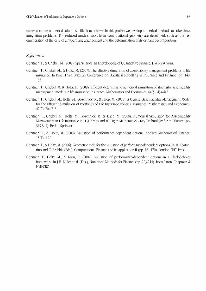
makes accurate numerical solutions difficult to achieve. In this project we develop numerical methods to solve theseintegration problems. For reduced models, tools from computational geometry are developed, such as the fastenumeration of the cells of a hyperplane arrangement and the determination of its orthant decomposition.

References

Gerstner, T., & Griebel, M. (2009). Sparse grids. In Encyclopedia of Quantitative Finance, J. Wiley & Sons.

Gerstner, T., Griebel, M., & Holtz, M. (2007). The effective dimension of asset-liability management problems in lifeinsurance. In Proc. Third Brazilian Conference on Statistical Modelling in Insurance and Finance (pp. 148-153).

Gerstner, T., Griebel, M. & Holtz, M. (2009). Efficient deterministic numerical simulation of stochastic asset-liabilitymanagement models in life insurance. Insurance: Mathematics and Economics, 44(3), 434-446.

Gerstner, T., Griebel, M., Holtz, M., Goschnick, R., & Haep, M. (2008). A General Asset-Liability Management Modelfor the Efficient Simulation of Portfolios of Life Insurance Policies. Insurance: Mathematics and Economics,42(2), 704-716.

Gerstner, T., Griebel, M., Holtz, M., Goschnick, R., & Haep, M. (2008). Numerical Simulation for Asset-LiabilityManagement in Life Insurance.In H.-J. Krebs and W. Jäger, Mathematics - Key Technology for the Future (pp.319-341). Berlin: Springer.

Gerstner, T., & Holtz, M. (2008). Valuation of performance-dependent options. Applied Mathematical Finance,15(1), 1-20.

Gerstner, T., & Holtz, M. (2006). Geometric tools for the valuation of performance-dependent options. In M. Costan-tino and C. Brebbia (Eds.), Computational Finance and its Application II (pp. 161-170). London: WIT Press.

Gerstner, T., Holtz, M., & Korn, R. (2007). Valuation of performance-dependent options in a Black-Scholesframework. In J.H. Miller et al. (Eds.), Numerical Methods for Finance (pp. 203-214). Boca Raton: Chapman &Hall/CRC.

CF2: Valuation of Performance Dependent Options 89

List of Publications 2006-2012

Peer-reviewedBuzdin, A., Logaschenko, D., & Wittum, G. (2008). IBLU Decompositions Based on Padé Approximants. Numerical Li-

near Algebra with Applications, 15(8), 717-746.

Eberhard, J. P., Wanner, A., & Wittum, G. (2006). NeuGen: A tool for the generation of realistic morphology of corti-cal neurons and neural networks in 3D. Journal of Neurocomputing, 70(1-3), 327-342.

Eberhard, J., Popovic, D., & Wittum, G. (2008). Numerical upscaling for the eddy-current model with stochastic mag-netic materials. Journal of Computational Physics, 227(8), 4244-4259.

Federico, S., Grillo, A., & Wittum, G. (2009). Considerations on Incompressibility in Linear Elasticity. Il Nuovo Cimen-to C, 32(1), 81-87.

Feuchter, D., Heisig, M., & Wittum, G. (2006). A geometry model for the simulation of drug diffusion through stra-tum corneum. Computing and Visualization in Science, 9(2), 117-130.

Fischer, T., Kirkilionis, M., Logashenko, D., & Wittum, G. (2006). Fast Numerical Integration for Simulation ofDisperse Systems. Mathematical Models and Methods in Applied Sciences, 16(12), 1987-2012.

Frolkovic, P., & Kacur, J. (2006). Semi-analytical solutions of contaminant transport equation with nonlinear sorptionin 1D, Computational Geosciences, 3(10), 279-290.

Frolkovic, P., & Mikula, K. (2007). High-resolution flux-based level set method. SIAM Journal on Scientific Compu-ting, 29(2), 579-597.

Frolkovic, P., & Mikula, K. (2007). Flux-based level set method: a finite volume method for evolving interfaces.Applied Numerical Mathematics, 57(4), 436-454.

Frolkovič, P., Mikula, K., Peyrieras, N., & Sarti, A. (2007). A counting number of cells and cell segmentation using ad-vection-diffusion equations. Kybernetika, 43(6), 817–829.

Frolkovic, P., Wehner, C. (2009). Flux-based level set method on rectangular grids and computations of first arrivaltime functions. Computing and Visualization in Science, 12(5), 297-306.

Frolkovic, P., Logashenko, D., & Wittum, G. (2008). Flux-based level set method for two-phase flows. In R. Eymard, J.-M. Herard (Eds.), Finite Volumes for Complex Applications V (pp. 415-422). London: ISTE and Wiley.

Gordner, A., & Wittum, G. (2007). Low Machnumber Aeroacoustics --- A direct one-grid approach. Journal of Numeri-cal Mathematics, 15(1), 7–29.

Grillo, A., Federico, S., Wittum, G., Imatani, S., Giaquinta, G., & Micunovic, M. V. (2009). Evolution of a Fibre-Reinfor-ced Growing Mixture. Il Nuovo Cimento C, 32(1), 97-119.

Grillo, A., Lampe, M., Logashenko, D., Stichel, S. & Wittum, G. (2012). Simulation of salinity- and thermohaline-dri-ven flow in fractured porous media. Journal of Porous Media, 15(5), 439-458.

Grillo, A., Lampe, M., & Wittum, G., (2010). Three-dimensional simulation of the thermohaline-driven buoyancy of abrine parcel. Computing and Visualization in Science, 13, 287-297.

Grillo, A., Lampe, M., & Wittum, G. (2011). Modelling and Simulation of Temperature-Density-Driven Flow and Ther-modiffusion in Porous Media. Journal of Porous Media, 14(8), 671-690.

Grillo, A., Logashenko, D., Stichel, S., & Wittum, G. (2010). Simulation of Density-Driven Flow in Fractured PorousMedia. Advances in Water Resources, 33(12), 1494-1507.

90 Publications

Grillo, A. & Wittum, G. (2010). Growth and mass transfer in multi-constituent biological materials. In T. Simos et al.(Eds.), ICNAAM 2010: International Conference of Numerical Analysis and Applied Mathematics 2010. Ameri-can Institute of Physics, Conference Proceedings. Volume 1281, pp. 355-359.

Grillo, A., Wittum, G., Giaquinta, G., & Micunovic, M. V. (2009). A Multiscale Analysis of Growth and Diffusion Dyna-mics in Biological Materials. International Journal of Engineering Science, 47(2), 261-283.

Hansen, S., Henning, A., Nägel, A., Heisig, M., Wittum, G., Neumann, D., Kostka, K. H., Zbytovska, J., Lehr, C. M., &Schäfer, U. F. (2008). In-silico model of skin penetration based on experimentally determined input parame-ters. Part I: Experimental determination of partition and diffusion coefficients. European Journal of Pharma-ceutics and Biopharmaceutics, 68(2), 352-367.

Hansen, S., Naegel, A., Heisig, M., Wittum, G., Neumann, D., Kostka, K., Meiers, P., Lehr, C. M., & Schaefer, U. F.(2009). The Role of Corneocytes in Skin Transport Revised - A Combined Computational and ExperimentalApproach. Pharmaceutical Research, 26, 1379-1397.

Hauser, A., Wittum, G. (2008). Analysis of Uniform and Adaptive LES in Natural Convection Flow. In J. Meyers et al.(Eds.), Quality and Reliability of Large-Eddy Simulations (pp. 105-116), Dordrecht: Springer.

Heumann, H., & Wittum, G (2009). The tree edit distance, a measure for quantifying neuronal morphology. Neuro-informatics, 7(3), 179-190.

Johannsen, K., Oswald, S., Held, R., & Kinzelbach, W. (2006). Numerical simulation of three-dimensional saltwater-freshwater fingering instabilities observed in a porous medium. Advances in Water Resources, 29(11), 1690-1704.

Johannsen, K. (2006). Multigrid Methods for Nonsymmetric Interior Penalty Discontinuous Galerkin Methods. Com-puting and Visualization in Science, to appear.

Jungblut, D., Queisser, G., & Wittum, G. (2012). Inertia Based Filtering of High Resolution Images Using a GPU Clus-ter. Computing and Visualization in Science, 14(4), 181-186.

Logashenko, D., Fischer, T., Motz, S., Gilles, E.-D., & Wittum, G. (2006). Simulation of Crystal Growth and Attritionin a Stirred Tank. Computing and Visualization in Science. 9(3), 175-183.

Mang, S. C., Logashenko, D., Gembris, D., Wittum, G., Grodd, W., & Klose, U. (2010). Diffusion Simulation BasedFiber Tracking using Time-of-Arrival Maps. Magnetic Resonance Materials in Physics, Biology and Medicine,23(5-6), 391-398.

Metzner, M., & Wittum, G. (2006). Computing low Mach-number flow by parallel adaptive multigrid. Computing andVisualization in Science, 9(4), 259-269.

Micunovic, M.V., Albertini, C., Grillo, A., Muha, I., Wittum, G., & Kudrjavceva, L. (2011). Two dimensional waves inquasi rate independent viscoplastic materials. Journal of Theoretical and Applied Mechanics, 38(1), 47-74.

Mo, Z., Zhang, A., & Wittum, G. (2009). Scalable Heuristic Algorithms fo the Parallel Execution of Data Flow AcyclicDigraphs. SIAM Journal on Scientific Computing, 31(5), 3626-3642.

Muha, I., Grillo, A., Heisig, M., Schönberg, M., Linke, B., & Wittum, G. (2012). Mathematical modeling of process li-quid flow and acetoclastic methanogenesis under mesophilic conditions in a two−phase biogas reactor. Bio-resource Technology, 106, 1-9.

Muha, I., Lenz, H., Feuchter, D., Handel, S., & Wittum, G. (2009). VVS eine Software zur Optimierung des Einlage-rungsprozesses in Horizontalsilos. Bornimer Agrartechnische Berichte, 68, 35-43.

Muha, I., Naegel, A., Stichel, S., Grillo, A., Heisig, M. & Wittum, G. (2011). Effective diffusivity in membranes with te-trakaidekahedral cells and implications for the permeability of human stratum corneum. Journal of Membra-ne Science 368(1-2), 18-25.

Publications 91

Muha, I., Stichel, S., Attinger, S., & Wittum, G. (2010). Coarse graining on arbitrary grids. SIAM Multiscale Modelingand Simulation 8(4), 1368-1382.

Nägel, A., Falgout, R. D., & Wittum, G. (2008). Filtering algebraic multigrid and adaptive strategies. Computing andVisualization in Science, 11(3), 159-167.

Naegel, A., Hansen, S., Neumann, D., Lehr, C., Schaefer, U. F., Wittum, G., & Heisig, M. (2008). In-silico model of skinpenetration based on experimentally determined input parameters. Part II: Mathematical modelling of in-vitrodiffusion experiments. Identification of critical input parameters. European Journal of Pharmaceutics and Bio-pharmaceutics, 68, 368-379.

Nägel, A., Heisig, M., & Wittum, G. (2009). A comparison of two- and three-dimensional models for the simulation ofthe permeability of human statum corneum. European Journal of Pharmaceutics and Biopharmaceutics, 72(2),332-338.

Naegel, A., Heisig, M., & Wittum, G. (2011). Computational modeling of the skin barrier. Methods Molecular Biology763, 1-32.

Naegel, A., Heisig, M., & Wittum, G. (in press). Detailed modeling of skin penetration - an overview. Advanced DrugDelivery Reviews.

Nägele, S., & Wittum, G. (2007). On the Influence of Different Stabilisation Methods for the Incompressible Navier-Stokes Equations. Journal of Computational Physics, 224(1), 100-116.

Queisser, G., Wiegert S. & Bading H. (2011). Structural dynamics of the nucleus: Basis for Morphology Modulation ofNuclear Calcium Signaling and Gene Transcription. Nucleus, 2(2), 98-104.

Queisser, G., Wittmann, M., Bading, H., & Wittum, G. (2008). Filtering, reconstruction and measurement of thegeometry of nuclei from hippocampal neurons based on confocal microscopy data. Journal of Biomedical Op-tics, 13(1), 014009.

Queisser, G. & Wittum, G. (2011). Investigating the Diffusion Properties of Nuclear Calcium. Biological Cybernetics,105(3-4), 211-216.

Reisinger, C., & Wittum, G. (2007). Efficient Hierarchical Approximation of High-Dimensional Option Pricing Prob-lems. SIAM Journal for Scientific Computing, 29(1), 440-458.

Sterz, O., Hauser, A., & Wittum, G. (2006). Adaptive Local Multigrid Methods for the Solution of Time Harmonic EddyCurrent Problems. IEEE Transactions on Magnetics, 42(2), 309-318.

Stichel, S., Logashenko, D., Grillo, A., Reiter, S., Lampe, M. & Wittum, G. (2012). Numerical methods for flow in frac-tured porous media. In J.M.P.Q. Delgado (Ed.), Heat and Mass Transfer in Porous Media (volume 13 of Advan-ced Structured Materials, pp. 83-113). Berlin: Springer.

Vogel, A., Xu, J. & Wittum, G. (2010). A generalization of the vertex-centered Finite Volume scheme to arbitrary highorder. Computing and Visualization in Science, 13(5), 221-228.

Voßen, C., Eberhard, J., & Wittum, G. (2007). Modeling and simulation for three-dimensional signal propagation inpassive dendrites. Computing and Visualization in Science, 10(2), 107-121.

Wittmann, M., Queisser, G., Eder, A., Bengtson, C. P., Hellwig, A., Wiegert, J. S., Wittum, G., & Bading, H. (2009).Synaptic activity induces dramatic changes in the geometry of the cell nucleus: interplay between nuclearstructure, histone H3 phosphorylation and nuclear calcium signaling. The Journal of Neuroscience, 29(47),14687-14700.

Xylouris, K., Queisser G., Wittum G. (2010). A Three-Dimensional Mathematical Model of Active Signal Processing inAxons. Computing and Visualization in Science, 13(8), 409-418.

92 Publications

Non peer reviewed

Atanackovic, T., Grillo, A., Wittum, G., & Zorica, D. (2010). An application of fractional calculus to growth mechanics.4th Workshop "Fractional Differentiation and its Applications" (FDA10), 18-20. X, 2010, Badajoz, Spain.

Eberhard, J., & Frolkovič, P. (2006). Numerical simulation of growth of an atherosclerotic lesion with a movingboundary. IWR-Preprint. Retrieved from http://archiv.ub.uni-heidelberg.de/volltextserver/volltexte/2006/6477/pdf/IWRpreprintEberhardFrolkovic2006.pdf

Frolkovič, P., Logashenko, D., Wehner, C., & Wittum, G. (2010). Finite volume method for two-phase flows usinglevel set formulation. Preprint 2010-10, Department of Mathematics and Descriptive Geometry, Slovak Uni-versity of Technology, Bratislava 2010.

Gordner, A., Nägele, S., & Wittum, G. (2006). Multigrid methods for large-eddy simulation. In W. Jäger et al. (Eds.),Reactive Flows, Diffusion and Transport. Berlin: Springer.

Grillo, A., Logashenko, D., & Wittum, G. (2009). Mathematical Modelling of a Fractured Porous Medium. Ober-wolfach Report No. 12/2009. Within the Mini-Workshop "Numerical Upscaling for Flow Problems: Theory andApplications." Mathematisches Forschungsinstitut Oberwolfach, 1.3.-7.3.2009.

Grillo, A., Logashenko, D., & Wittum, G. (2009). Study of Transport Problem in a Two-Dimensional Porous Medium.In the Proceedings of the COSSERAT+100 International Conference on the Legacy of "Théorie des CorpsDéformables" by Eugéne and Francois Cosserat in the centenary of iths publication. École des Ponts Paris-Tech, 15th-17th of July 2009.

Jungblut, D., Karl, S., Mara, H., Krömker, S., & Wittum, G. (2009). Automated GPU-based Surface Morphology Recon-struction of Volume Data for Archeology. SCCH 2009.

Micunovic, M. V., Grillo, A., Muha, I., & Wittum, G. (2009). Two Dimensional Plastic Waves in Quasi Rate Indepen-dent Viscoplastic Materials. In the Proceedings of the ESMC2009, 7th EUROMECH, Lisbon, Portugal, 7th-11thSeptember 2009.

v. Rohden, C., Hauser, A., Wunderle, K., Ilmberger, J., Wittum, G., & Roth, K. (2006). Lake dynamics: observation andhigh-resolution numerical simulation. In W. Jäger et al. (Eds.), Reactive Flows, Diffusion and Transport. Ber-lin: Springer.

Submitted papers and papers in preparationBuzdin, A., Logashenko, D., & Wittum, G. (2009). Frequency Filtering in the Iterative Solution of Eigenvalue Prob-

lems. Manuscript submitted for publication.

Frolkovic, P., & Lampe, M., & Wittum, G. (2011). Numerical simulation of contaminant transport in groundwaterusing software tools r3t. Manuscript submitted for publication.

Frolkovic, P., Logashenko, D., Wehner, C., Wittum, G. (2009). Finite volume method for two-phase flows using levelset formulation. Manuscript submitted for publication.

Frolkovič, P., Logashenko, D., Wehner, C., & Wittum, G. (2011). Flux-based level set method and applications on un-structured grids. Manuscript submitted for publication.

Grillo, A., & Wittum, G. (2010). Considerations on growth and transfer processes in multi-constituent materials. Ma-nuscript submitted for publication.

Publications 93

Hoffer, M., Poliwoda, C., & Wittum, G. (2011). Visual Reflection Library. A Framework for Declarative GUI Program-ming on the Java Platform. Manuscript in preparation.

Johannsen, K., & Wittum, G. (2006). A SOR-type smoother for strongly non-symmetric positive definite matrices. Un-published.

Karl, S., Jungblut, D., Mara, H., Wittum, G., & Krömker, S. (2010). Insights in Manufacturing Techniques of AncientPottery: Industrial X-Ray Computed Tomography as a Tool in the Examination of Cultural Material in Muse-ums. Manuscript submitted for publication.

Knodel, M., Queisser, G., Geiger, R., Ge, L. H., Bucher, D., Grillo, A., Schuster C.M. & Wittum, G. (2010). BoutonSizes are Tuned to Best Fit their Physiological Performances. Manuscript submitted for publication.

Micunovic, M.V., Albertini, C., Grillo, A., Muha, I., & Wittum, G. (2009). Two dimensional waves in quasi rate indepen-dent viscoplastic materials. Manuscript submitted for publication.

Muha, I., Heisig, M., Schönberg, M., Linke, B., Wittum, G. (2011). Methanogenesis from acetate under mesophiliccondition in a biogas reactor. In preparation.

Muha, I., Stichel, S., Naegel, A., Heisig, M., & Wittum, G. (2009). Using homogenization theory to calculate an effecti-ve diffusion tensor for human stratum corneum with tetrakaidekahedral geometry. In preparation.

Muha, I., Zielonka, S., Lemmer, A., Schönberg, M., Linke, B., & Wittum, G. (2012). Do two stage biogas reactors sepe-rate the processes? Bioresource Technology. In preparation.

Naegel A., Hahn T., Lehr C.-M., Schaefer U.F., Heisig M., & Wittum G. (2012). Finite dose skin penetration: Concen-tration depth profiles - Comparison between experiment and simulation. Manuscript submitted for publicati-on.

Naegel A., Heisig, M., Wittum, G., K.H. Schaller, H. Drexler, & Korinth, G. Prospective evaluation of a sophisticatedpredictive mathematical model to simulate the percutaneous penetration of caffeine. Manuscript submittedfor publication.

Queisser, G. & Wittum, G. (2010). Investigating the Diffusion Properties of Nuclear Calcium. Manuscript submittedfor publication.

Reiter, S., Logashenko, D., Stichel, S., Wittum, G., & Grillo, A. (2012). Models and simulations of variable-density flowin fractured porous media. Manuscript submitted for publication.

Schröder, P., Gerstner, T., & Wittum, G. (2012). Taylor-like ANOVA Expansion for high dimensional Problems in Fi-nance. Manuscript submitted for publication.

Selzer D., T. Hahn T., Naegel A., Heisig M., Neumann D., Kostka K.H., Lehr C.M., Schaefer U.F., & Wittum G. (2012).Finite dose skin mass balance including the lateral part - Comparison between experiment, pharmacokineticmodeling, and diffusion models. Manuscript submitted for publication.

Wolf, S., Grein, S., & Queisser, G. (2011). Employing NeuGen 2.0 to automatically generate realistic morphologies ofhippocampal neurons and neural networks in 3D. Manuscript submitted for publication.

Wolf, S., Wittum, G. & Queisser, G. (2010). NeuGen3D: The CA1 Region. In preparation.

94 Publications