1

GEM-MACH-PAH (rev2488): a new high-resolution chemistry transport model for North American PAHs and benzene

Cynthia H. Whaley, Elisabeth Galarneau, Paul A. Makar, Ayodeji Akingunola, Wanmin Gong, Sylvie Gravel, Michael D. Moran, Craig Stroud, Junhua Zhang, and Qiong Zheng

SUPPLEMENTAL MATERIAL CONTENTS A: Measurement Sites ………………………………………………….. 2 B: Gas-particle partitioning analysis ………………………….……….. 6

B.1: Discussion of Junge-Pankow ………………………….. 6 B: Derivation of m = -1 for Junge-Pankow ………………. 8 B.2: Derivation of new KSW for Dachs-Eisenreich scheme ….. 9

C: Verification of PAH mobile EFs from other sources ……………. … 11 D: Species-specific constants needed for scavenging …………….…… 12 E: Additional Hamilton Analysis ………………………………….. 13 References ………………………………………………………….. 14

2 A: Table of measurement sites Table A.1: Benzene and PAH network measurement sites in the Pam Am model domain. Note that NATTS documentation provides site IDs, but not names, therefore the first column provides the state where the particular site resides, and cities/towns were manually looked up and added for those sites that have PAH measurements.

Site name or State Site ID Latitude Longitude measurement IADN sites

University of Toronto, ON UOT 43.8725 -79.18833 PAH wet dep St Clair, ON STC 42.53594 -82.38978 PAH wet dep Burlington, ON BUR 43.36889 -79.87028 PAH wet dep Burnt Island, ON BNT 45.82833 -82.94806 PAHs Point Petre, ON PPT 43.84278 -77.15361 PAHs/PAH wet

dep Sturgeon Point, NY STP 42.69306 -79.055 PAHs/PAH wet

dep Cleveland, OH CLV 41.49214 -81.67853 PAHs/PAH wet

dep Sleeping Bear Dunes, MI SBD 44.76111 -86.0586 PAHs Chicago IIT, IL IIT 41.83444 -87.6247 PAHs

NAPS sites College and South, Windsor, ON

60211 42.29289 -83.0731 PAHs, benzene

Gage Institute, Toronto, ON

60427 43.65822 -79.3972 PAHs, benzene

Etobicoke South (Toronto Kipling), ON

60435 43.61076 -79.5219 PAHs, benzene

Elgin and Kelly, Hamilton, ON

60512 43.25778 -79.8617 PAHs, benzene

Experimental Farm, Simcoe, ON

62601 42.8569 -80.2703 PAHs, benzene

Egbert, ON 64401 44.23111 -79.7831 PAHs, benzene Point Petre, ON 64601 43.84278 -77.1536 PAHs, benzene Burnt Island, ON 65501 45.82833 -82.9481 PAHs, benzene

NATTS sites Middletown, OH 390170003 39.4938 -84.3543 benzene OH 390350038 41.47701 -81.6824 benzene OH 390350068 41.45478 -81.6344 benzene OH 390350069 41.519 -81.6378 benzene OH 390350071 41.49251 -81.67 benzene OH 390490034 40.00274 -82.9944 benzene OH 390515502 41.55002 -84.1365 benzene OH 390610014 39.19433 -84.479 benzene OH 390610044 39.13837 -84.7116 benzene

3 OH 390610045 39.17093 -84.5287 benzene OH 390610046 39.11412 -84.5363 benzene OH 390810017 40.36644 -80.6156 benzene Ironton, OH 390875503 38.51814 -82.6688 PAHs, benzene Franklin Furnace, OH 391450020 38.60934 -82.8225 PAHs, benzene Franklin Furnace, OH 391450021 38.60066 -82.8296 PAHs, benzene Franklin Furnace, OH 391450022 38.58808 -82.8348 PAHs, benzene Warren, OH 391555504 41.23506 -80.8127 PAHs, benzene MI 260330901 46.49361 -84.3642 benzene MI 261110951 43.60917 -84.2106 benzene MI 261110953 43.59139 -84.2094 benzene MI 261110955 43.58944 -84.2211 benzene MI 261110959 43.57419 -84.3216 benzene MI 261630015 42.30279 -83.1065 benzene Dearborn, MI 261630033 42.30754 -83.1496 PAHs, benzene MI 261635502 42.35059 -83.0524 benzene Liberty, PA 420030064 40.32377 -79.8681 PAHs, benzene Clairton, PA 420033007 40.29434 -79.8853 PAHs, benzene Kennedy Township, PA 420035503 40.49435 -80.0964 PAHs, benzene PA 420450002 39.83556 -75.3725 benzene PA 420710007 40.04667 -76.2833 benzene PA 420770004 40.61194 -75.4325 benzene PA 420910005 40.19255 -75.4575 benzene PA 421010004 40.00889 -75.0978 benzene PA 421010014 40.04962 -75.2408 benzene PA 421010047 39.94465 -75.1652 benzene PA 421010055 39.92287 -75.1869 benzene PA 421010063 39.88294 -75.2197 benzene PA 421010136 39.9275 -75.2228 benzene PA 421190001 40.95517 -76.8819 benzene PA 421250005 40.14667 -79.9022 benzene PA 420010001 39.92002 -77.3097 benzene PA 420030031 40.44337 -79.9903 benzene Philadelphia, PA 421010449 39.9825 -75.0831 PAHs Buffalo, NY 360291013 42.98844 -78.9186 PAHs, benzene Rochester, NY 360551007 43.1462 -77.5481 PAHs, benzene NY 360050133 40.8679 -73.8781 benzene NY 360095501 42.08506 -78.4336 benzene NY 360291007 42.7273 -78.8498 benzene NY 360291014 42.99813 -78.8993 benzene NY 360310003 44.39308 -73.8589 benzene NY 360470118 40.69545 -73.9277 benzene

4 NY 360610115 43.84955 -79.9357 benzene NY 360632008 43.08218 -79.0011 benzene NY 360810124 40.73614 -73.8216 benzene NY 360831003 42.73194 -73.6891 benzene NY 360850111 40.58027 -74.1983 benzene NY 360850132 40.58056 -74.1518 benzene NY 361030009 40.82799 -73.0575 benzene New York, NY 360050110 40.81616 -73.9021 PAHs, benzene CT 90019003 41.11833 -73.3367 benzene CT 90031003 41.78472 -72.6317 benzene CT 90090027 41.3014 -72.9029 benzene DE 100031008 39.5778 -75.6107 benzene DE 100032004 39.73944 -75.5581 benzene NJ 340155501 39.83709 -75.244 benzene NJ 340210005 40.28309 -74.7427 benzene NJ 340230006 40.47282 -74.4224 benzene NJ 340230011 40.46218 -74.4294 benzene NJ 340273001 40.78763 -74.6763 benzene NJ 340390004 40.64144 -74.2084 benzene NJ 340395502 40.65205 -74.1999 benzene MD 240053001 39.31083 -76.4744 benzene MD 240330030 39.05528 -76.8783 benzene MD 245100006 39.34056 -76.5822 benzene MD 245100040 39.29806 -76.6047 benzene Washington, DC 110010043 38.92185 -77.0132 PAHs, benzene Providence, RI 440070022 41.80795 -71.415 PAHs, benzene RI 440030002 41.61524 -71.72 benzene RI 440070026 41.87467 -71.38 benzene RI 440071010 41.84157 -71.3608 benzene NH 330110020 42.99578 -71.4625 benzene NH 330111011 42.71866 -71.5224 benzene NH 330115001 42.86175 -71.8784 benzene NH 330150014 43.07533 -70.748 benzene MA 250092006 42.47464 -70.9708 benzene MA 250130008 42.19438 -72.5551 benzene MA 250213003 42.21177 -71.114 benzene MA 250250041 42.31737 -70.9684 benzene Boston, MA 250250042 42.32944 -71.0825 PAHs, benzene Northbrook, IL 170314201 42.14 -87.7992 PAHs, benzene O'Hare airport, Chicago, IL 170313103 41.96519 -87.8763 benzene Underhill, VT 500070007 44.52839 -72.8688 PAHs, benzene VT 500070014 44.4762 -73.2106 benzene

5 VT 500210002 43.60806 -72.9828 benzene East Chicago, IN 180895503 41.64921 -87.4475 PAHs, benzene Gary, IN 180895504 41.5997 -87.3443 PAHs, benzene IN 180190009 38.27668 -85.7638 benzene IN 180855502 41.23898 -85.8321 benzene IN 180890022 41.60668 -87.3047 benzene IN 180890023 41.65274 -87.4396 benzene IN 180890030 41.6814 -87.4947 benzene IN 180970078 39.8111 -86.1145 benzene IN 180970084 39.75885 -86.1154 benzene IN 181270024 41.61756 -87.1993 benzene IN 181570008 40.43164 -86.8525 benzene IN 181630016 37.97444 -87.5323 benzene Follansbee, WV 540095501 40.33564 -80.5953 PAHs, benzene WV 540390010 38.3456 -81.6283 benzene WV 540610003 39.64937 -79.9209 benzene WV 540690010 40.11488 -80.701 benzene Richmond, VA 510870014 37.55655 -77.4004 PAHs, benzene VA 510330001 38.20087 -77.3774 benzene VA 510590030 38.77335 -77.1047 benzene VA 516700010 37.28962 -77.2918 benzene VA 518100008 36.84188 -76.1812 benzene OH 391450020 38.60934 -82.82251 N/A OH 391450021 38.60066 -82.82964 N/A

6 B: Gas-particle partitioning analysis B.1 Justification for exclusion of Junge-Pankow partitioning from GEM-MACH-PAH Junge-Pankow partitioning (JP) is based on Langmuir adsorption (Langmuir, 1918). It expresses partitioning as a particulate fraction ϕk for each PAH species, k:

𝜙𝜙𝑘𝑘 = 𝑐𝑐𝑐𝑐𝑝𝑝𝐿𝐿,𝑘𝑘𝑜𝑜 +𝑐𝑐𝑐𝑐

, (B.1.1)

where ϕk is equal to the particulate concentration divided the total PAH species concentration. When ϕk =1, all of the concentration is in the particle phase, and none is in the gas phase, while ϕk =0 means all of the PAH is in the gas phase. θ is the total dry aerosol-particle surface area (m2), pL,k

o is the subcooled liquid saturated vapor pressure per PAH species, and c is a constant that depends on the chemical species and the temperature (Junge, 1977). The vapor pressure is calculated using the relation:

𝑙𝑙𝑙𝑙𝑙𝑙𝐾𝐾𝑝𝑝,𝑘𝑘 = 𝑚𝑚𝐾𝐾𝑙𝑙𝑙𝑙𝑙𝑙𝑝𝑝𝐿𝐿,𝑘𝑘𝑜𝑜 + 𝑏𝑏𝐾𝐾 (B.1.2)

where mp,k and bp,k come from Offenberg and Baker (1999)'s supporting information for PAHs. Figure B.1b shows sample plots of ϕk vs log pL,k

o. These examples show how the measurements (blue crosses) differ from the JP model (purple points and black line), which requires that mK = -1 (see next section for the derivation of this). The JP formulation does not allow for improvement given the mK = -1 constraint. Therefore, the Dachs-Eisenreich formulation is examined next.

7

Figure B.1: (a) Chicago (taken as example) modelled (from AURAMS-PAH) and measured logKp vs logp◦ for all 7 PAHs, and their linear fits for 2002 data. Thick black line indicates the median linear fit. a(i) original JP and DE partitioning scheme, a(ii) all measurements, a(iii): only those measurements where all 7 PAHs were measured. (b) Particulate fraction (φ) vs logpL

o for AURAMS-PAH model and 2002 measurement samples from four sites. The Junge-Pankow model is shown for 7 PAH species in purple points, and Eq. (B.1.1) as a black line. The measurements are shown as blue crosses.

(a)

(b)

(i) (ii) (iii)

8 B: Derivation of m = -1 for JP formulation, starting with Eq. (B.1.1)

9 B.2: Derivation of improved physico-chemical parameters for use with Dachs-Eisenreich partitioning The Dach-Eisenreich expression for Kp is:

𝐾𝐾𝑝𝑝,𝑘𝑘 = 10−12 �1.5𝑓𝑓𝑂𝑂𝑂𝑂𝜌𝜌𝑜𝑜𝑐𝑐𝑜𝑜

𝐾𝐾𝑂𝑂𝑂𝑂,𝑘𝑘 + 𝑓𝑓𝐸𝐸𝑂𝑂𝐾𝐾𝑆𝑆𝑂𝑂,𝑘𝑘�

= 10−12𝑓𝑓𝐸𝐸𝑂𝑂𝐾𝐾𝑆𝑆𝑂𝑂,𝑘𝑘 + 1.5 × 10−12 𝑓𝑓𝑂𝑂𝑂𝑂𝜌𝜌𝑜𝑜𝑜𝑜𝑜𝑜

𝐾𝐾𝑂𝑂𝑂𝑂,𝑘𝑘 (B.2.1)

where fOC and fEC are the organic and elemental carbon fractions respectively, the 1.5 factor is an estimate to convert organic carbon to orgamic material, ρoct is the density of octanol, the octanol-air partitioning coefficient, KOA,k, is related to temperature:

𝐾𝐾𝑂𝑂𝑂𝑂,𝑘𝑘 = 10𝑚𝑚𝑂𝑂𝑂𝑂,𝑘𝑘

𝑇𝑇 +𝑏𝑏𝑂𝑂𝑂𝑂,𝑘𝑘 (B.2.2) where mOA,k and bOA,k are taken from Odabasi et al (2006), and the soot-air partitioning coefficient, KSA,k, is related to the soot-water and air-water partitioning coefficients:

𝐾𝐾𝑆𝑆𝑂𝑂,𝑘𝑘 = 𝐾𝐾𝑆𝑆𝑆𝑆,𝑘𝑘𝑒𝑒−𝐾𝐾𝑂𝑂𝐴𝐴.𝑘𝑘

= 𝐾𝐾𝑆𝑆𝑆𝑆,𝑘𝑘𝑒𝑒−(

𝑚𝑚𝑂𝑂𝐴𝐴,𝑘𝑘𝑇𝑇 +𝑏𝑏𝑂𝑂𝐴𝐴,𝑘𝑘), (B.2.3)

where mAW,k and bAW,k are from Sander (1999) and Bamford et al (1999). An update for bAW,k was calculated from the 25oC KAW,k, values given in Ma et al (2010) using Eq. (B.2.3). KOA,k and ρoct are also well-known, and make the second term in Eq. (B.2.1) four orders of magnitude smaller than the first term. The KSW,k values (in Eq. (B.2.3)) are highly uncertain. Using our new AURAMS-PAH model-measurement comparisons, we have determined new KSW,k values that would improve the DE particulate fraction representation. Fig. B.1a shows logKp,k vs logpL,k for each 2002 Chicago measurement sample (of multiple PAH species) in the Galarneau et al (2014) study (these are measurements of up to 7 PAH species in the gas and particle phases, thus for each PAH, the gas-particle partitioning coefficient (Kp can be plotted against that PAH's vapour pressure), and their linear fits. Eq. (B.1.2) governs the data relationship, but the observations have more spread in slope than the AURAMS-PAH model is capable of representing (shown in Figure B.1a). Using the JP or DE formulation, the model can not represent the variability in the slope, however, unlike the JP formulation, the DE model slope (mK) can be altered to better match observations. The modeled slope, at -1, was too steep compared to the measurements (Fig. B.1a (i) vs. (ii) and (iii)). Note that most of the measured samples did not have BaP measurements, as this species is difficult to measure unless its

10 concentrations are high. Therefore, the median line from the fits that include all samples (thick black line in Fig. B.1a(ii)) does not represent BaP measurements well. BaP points tend to fall well below the median line (see circle in Fig. B.1a(ii)). Therefore, we selected only samples that had all seven PAHs measured (from all sites -- shown in Fig. B.1a(iii) for Chicago samples), and calculated a median line from these linear fits. This median line better represents the slope and intercept of all PAHs, including BaP. Chicago was shown as an example, however, the original modelled slopes for all sites were too steep (too negative), and the intercepts too low. Therefore, to adjust KSW,k, we utilize the median mk and bk from the 2002 North American measurements, described above. First, we substitute Eq. (B.1.2) into Eq. (1) to get:

log𝐾𝐾𝑝𝑝,𝑘𝑘 = 𝑚𝑚𝐾𝐾 �𝑚𝑚𝑝𝑝,𝑘𝑘

𝑇𝑇+ 𝑏𝑏𝑝𝑝,𝑘𝑘� + 𝑏𝑏𝐾𝐾

= 𝑚𝑚𝐾𝐾𝑚𝑚𝑝𝑝,𝑘𝑘

𝑇𝑇+ 𝑚𝑚𝐾𝐾𝑏𝑏𝑝𝑝,𝑘𝑘 + 𝑏𝑏𝐾𝐾 (B.2.4)

Fig. 2a shows the all-site (2002) ensemble of AURAMS-PAH model-over-measured logKp and (b) particulate fraction, in green. The `` adjusted model" -- which is a actually just a re-calculation of logKp from Eq. (B.2.4), using AURAMS-PAH temperature and the median measured mK and bK – is plotted in purple. We then substitute Eq. (B.2.3) into Eq. (B.2.1), dropping the second term in equation (B.2.1) because we have verified that it is negligible, and because doing so greatly simplifies the math, to get:

𝐾𝐾𝑝𝑝,𝑘𝑘 = 10−12𝑓𝑓𝐸𝐸𝑂𝑂𝐾𝐾𝑆𝑆𝑆𝑆,𝑘𝑘𝑒𝑒−(

𝑚𝑚𝑂𝑂𝐴𝐴,𝑘𝑘𝑇𝑇 +𝑏𝑏𝑂𝑂𝐴𝐴,𝑘𝑘) (B.2.5)

We set the right-hand-side of Eq. (B.2.4) equal to the log of Kp,k from Eq. (B.2.5) to get our new KSW,k expression:

𝐾𝐾𝑆𝑆𝑆𝑆,𝑘𝑘 = 10(𝑚𝑚𝐾𝐾𝑚𝑚𝑝𝑝,𝑘𝑘

𝑇𝑇 +𝑚𝑚𝐾𝐾𝑏𝑏𝑝𝑝,𝑘𝑘+𝑏𝑏𝐾𝐾+12)

𝑓𝑓𝐸𝐸𝑂𝑂𝑒𝑒−(𝑚𝑚𝑂𝑂𝐴𝐴,𝑘𝑘

𝑇𝑇 +𝑏𝑏𝑂𝑂𝐴𝐴,𝑘𝑘) (B.2.6)

Eq. (B.2.6) is thus a means of describing PAH partitioning based on measurements, and the resulting KSW,k values are summarized in Table 1. The new KSW,k values will go into equation B.2.3 to give new KSA,k values that will go into equation B.2.1, which does the PAH partitioning in the model.

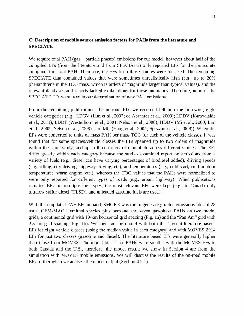
11 C: Description of mobile source emission factors for PAHs from the literature and SPECIATE We require total PAH (gas + particle phases) emissions for our model, however about half of the compiled EFs (from the literature and from SPECIATE) only reported EFs for the particulate component of total PAH. Therefore, the EFs from those studies were not used. The remaining SPECIATE data contained values that were sometimes unrealistically high (e.g., up to 20% phenanthrene in the TOG mass, which is orders of magnitude larger than typical values), and the relevant databases and reports lacked explanations for these anomalies. Therefore, none of the SPECIATE EFs were used in our determination of new PAH emissions. From the remaining publications, the on-road EFs we recorded fell into the following eight vehicle categories (e.g., LDGV (Lim et al., 2007; de Abrantes et al., 2009); LDDV (Karavalakis et al., 2011); LDDT (Westerholm et al., 2001; Nelson et al., 2008); HDDV (Mi et al., 2000; Lim et al., 2005; Nelson et al., 2008); and MC (Yang et al., 2005; Spezzano et al., 2008)). When the EFs were converted to units of mass PAH per mass TOG for each of the vehicle classes, it was found that for some species/vehicle classes the EFs spanned up to two orders of magnitude within the same study, and up to three orders of magnitude across different studies. The EFs differ greatly within each category because the studies examined report on emissions from a variety of fuels (e.g., diesel can have varying percentages of biodiesel added), driving speeds (e.g., idling, city driving, highway driving, etc), and temperatures (e.g., cold start, cold outdoor temperatures, warm engine, etc.), whereas the TOG values that the PAHs were normalized to were only reported for different types of roads (e.g., urban, highway). When publications reported EFs for multiple fuel types, the most relevant EFs were kept (e.g., in Canada only ultralow sulfur diesel (ULSD), and unleaded gasoline fuels are used). With these updated PAH EFs in hand, SMOKE was run to generate gridded emissions files of 28 usual GEM-MACH emitted species plus benzene and seven gas-phase PAHs on two model grids, a continental grid with 10-km horizontal grid spacing (Fig. 1a) and the “Pan Am” grid with 2.5-km grid spacing (Fig. 1b). We then ran the model with both the ``recent-literature-based" EFs for eight vehicle classes (using the median value in each category) and with MOVES 2014 EFs for just two classes (gasoline and diesel). The literature based EFs were generally higher than those from MOVES. The model biases for PAHs were smaller with the MOVES EFs in both Canada and the U.S., therefore, the model results we show in Section 4 are from the simulation with MOVES mobile emissions. We will discuss the results of the on-road mobile EFs further when we analyze the model output (Section 4.2.1).

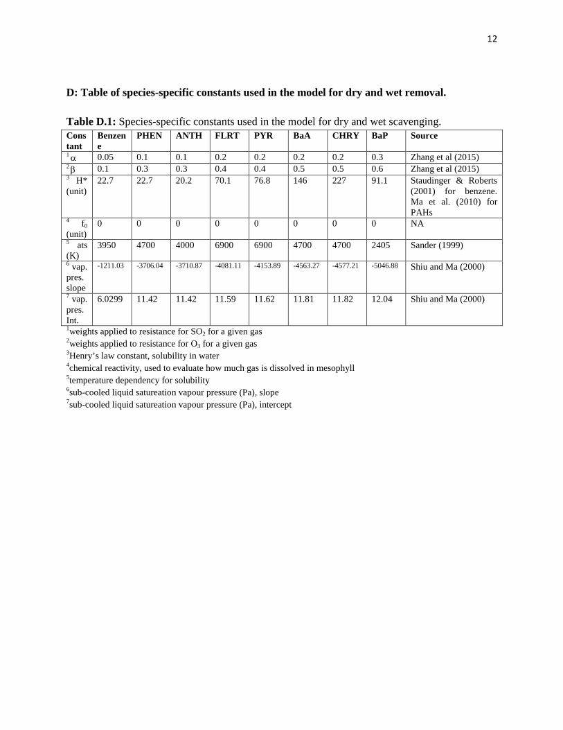
12 D: Table of species-specific constants used in the model for dry and wet removal. Table D.1: Species-specific constants used in the model for dry and wet scavenging. Constant

Benzene

PHEN ANTH FLRT PYR BaA CHRY BaP Source

1 α 0.05 0.1 0.1 0.2 0.2 0.2 0.2 0.3 Zhang et al (2015) 2 β 0.1 0.3 0.3 0.4 0.4 0.5 0.5 0.6 Zhang et al (2015) 3 H* (unit)

22.7 22.7 20.2 70.1 76.8 146 227 91.1 Staudinger & Roberts (2001) for benzene. Ma et al. (2010) for PAHs

4 f0 (unit)

0 0 0 0 0 0 0 0 NA

5 ats (K)

3950 4700 4000 6900 6900 4700 4700 2405 Sander (1999)

6 vap. pres. slope

-1211.03 -3706.04 -3710.87 -4081.11 -4153.89 -4563.27 -4577.21 -5046.88 Shiu and Ma (2000)

7 vap. pres. Int.

6.0299 11.42 11.42 11.59 11.62 11.81 11.82 12.04 Shiu and Ma (2000)

1weights applied to resistance for SO2 for a given gas 2weights applied to resistance for O3 for a given gas 3Henry’s law constant, solubility in water 4chemical reactivity, used to evaluate how much gas is dissolved in mesophyll 5temperature dependency for solubility 6sub-cooled liquid satureation vapour pressure (Pa), slope 7sub-cooled liquid satureation vapour pressure (Pa), intercept

13 E: Hamilton PAHi/PM2.5 analysis

Figure E.1: Left: Measured and modelled and concentration ratios of FLRT/PM2.5 in Hamilton, Ontario for two-week summer 2009 period. Right: Their differences and ratios. Note that spatial pattern in model bias is missing.

Figure E.2: Same as Fig. E.1, but for PM2.5 concentrations. Note that modelled PM2.5 is biased high, and is causing the spatial pattern seen in the PAH bias (cf. Fig. 4a).

14

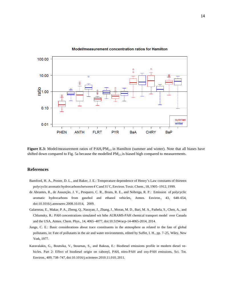
Figure E.3: Model/measurement ratios of PAHi/PM2.5 in Hamilton (summer and winter). Note that all biases have shifted down compared to Fig. 5a because the modelled PM2.5 is biased high compared to measurements. References

Bamford, H. A., Poster, D. L., and Baker, J. E.: Temperature dependence of Henry’s Law constants of thirteen

polycyclic aromatic hydrocarbons between 4◦C and 31◦C, Environ. Toxic. Chem., 18, 1905–1912, 1999. de Abrantes, R., de Assunção, J. V., Pesquero, C. R., Bruns, R. E., and Nóbrega, R. P.: Emission of polycyclic

aromatic hydrocarbons from gasohol and ethanol vehicles, Atmos. Environ., 43, 648–654,

doi:10.1016/j.atmosenv.2008.10.014, 2009.

Galarneau, E., Makar, P. A., Zheng, Q., Narayan, J., Zhang, J., Moran, M. D., Bari, M. A., Pathela, S., Chen, A., and

Chlumsky, R.: PAH concentrations simulated wit hthe AURAMS-PAH chemical transport model over Canada

and the USA, Atmos. Chem. Phys., 14, 4065–4077, doi:10.5194/acp-14-4065-2014, 2014.

Junge, C. E.: Basic considerations about trace constituents in the atmosphere as related to the fate of global

pollutants, in: Fate of pollutants in the air and water environments, edited by Suffet, I. H., pp. 7–25, Wiley, New

York, 1977.

Karavalakis, G., Boutsika, V., Stournas, S., and Bakeas, E.: Biodiesel emissions profile in modern diesel ve-

hicles. Part 2: Effect of biodiesel origin on cabonyl, PAH, nitro-PAH and oxy-PAH emissions, Sci. Tot.

Environ., 409, 738–747, doi:10.1016/j.scitotenv.2010.11.010, 2011.

15

Langmuir, I.: The adsorption of gases on plane surfaces of glass, mica, and platinum, J. Am. Chem. Soc., 40,

1361–1402, 1918.

Lim, M. C. H., Ayoko, G. A., Morawaska, L., Ristovski, Z. D., and Jayaratne, E. R.: Effect of fuel composition and

engine operating conditions on polycyclic aromatic hydrocarbon emissions from a fleet of heavy-duty diesel

buses, Atmos. Environ., 39, 7836–7848, doi:10.1016/j.atmosenv.2005.09.019, 2005.

Lim, M. C. H., Ayoko, G. A., Morawaska, L., Ristovski, Z. D., and Jayaratne, E. R.: Influence of fuel com-

position on polycyclic aromatic hydrocarbon emissions from a fleet of in-service passenger cars, Atmos.

Environ., 41, 150–160, doi:10.1016/j.atmosenv.2006.07.044, 2007.

Ma, Y.-G., Lei, Y. D., Xiao, H., Wania, F., and Wang, W.-H.: Critical review and recommended values for the

physical-chemical property data of 15 polycyclic aromatic hydrocarbons at 25◦C, J. Chem. Eng. Data, 55, 819–825, doi:10.1021/je900477x, 2010.

Mi, H.-H., Lee, W.-J., Chen, C.-B., Yang, H.-H., and Wu, S.-J.: Effect of fuel aromatic content on PAH emission

from a heavy-duty diesel engine, Chemosphere, 41, 1783–1790, 2000.

Nelson, P. F., Tibbett, A. R., and Day, S. J.: Effects of vehicle type and fuel quality on real world toxic emissions

from diesel vehicles, Atmos. Environ., 42, 5291–5303, doi:10.1016/j.atmosenv.2008.02.049, 2008.

Odabasi, M., Cetin, E., and Sofuoglu, A.: Determination of octanol-air partition coefficients and supercooled

liquid vapor pressures of PAHs as a function of temperature: application to gas-particle partitioning in an

urban atmosphere, Atmos. Environ., 40, 6615–6625, doi:10.1016/j.atmosenv.2006.05.051, 2006.

Offenberg, J. H. and Baker, J. E.: Aerosol size distributions of polycyclic aromatic hydrocarbons in urban and

over-water atmospheres, Environ. Sci. Technol., 33, 3324–3331, doi:10.1021/es990089c, 1999.

Sander, R.: Modeling atmospheric chemistry: interactions between gas-phase species and liquid cloud/aerosol

particles, Surveys in Geophysics, 20, 1–31, 1999.

Shiu, W.-Y., Ma, K.-C.: Temperature dependence of physical-chemical properties of selected chemicals of

environmental interest. I. Mononuclear and polynuclear aromatic hydrocarbons, J. Phys. Chem. Ref. Data, 29,

no. 1, 41-130, doi:10.1063/1.556055, 2000.

Spezzano, P., Picini, P., Cataldi, D., Messale, F., and Manni, C.: Particle- and gas-phase emissions of polycyclic

aromatic hydrocarbons from two-stroke, 50-cm3 mopeds, Atmos. Environ., 42, 4332–4344,

doi:10.1016/j.atmosenv.2008.01.008, 2008.

Staudinger, J., Roberts, P. V.: A critical compilation of Henry’s law constant temperature dependence relations for

organic compounds, Chemosphere, 44, 561-576, doi:10.1016/S0045-6535(00)00505-1, 2001.

Westerholm, R., Christensen, A., Törnqvist, M., Ehrenberg, L., Rannug, U., Sjögren, M., Rafter, J., Soontjens, C.,

Almén, J., and Grägg, K.: Comparison of exhaust emissions from Swedish environmental classified diesel fuel

(MK1) and European program on emissions, fuels, and engine technologies (EPEFE) Reference fuel: a

chemical and biological characterization, with viewpoints on cancer risk, Environ. Sci. Technol., 35, 1748–

1754, doi:10.1021/es000113i, 2001.

Yang, H.-H., Chien, S.-M., Chao, M.-R., and Lin, C.-C.: Particle size distribution of polycyclic aromatic hydro-

carbons in motorcycle exhaust emissions, J. Haz. Mat., B125, 154–159, doi:10.1016/j.jhazmat.2005.05.019,

2005.

Zhang, L., Cheng, I., Muir, D., Charland, J.-P.: Scavenging ratios of polycyclic aromatic compounds

16

in rain and snow in the Athabasca oil sands region, Atmos. Chem. Phys., 15, 1421-1434, doi: 10.5194/acp-15-

1421-2015, 2015.