Functions of bounded variation on compact subsets of...
32
Functions of bounded variation on compact subsets of the plane Brenden Ashton and Ian Doust Abstract A major obstacle in extending the theory of well-bounded oper- ators to cover operators whose spectrum is not necessarily real has been the lack of a suitable variation norm applicable to functions defined on an arbitrary nonempty compact subset σ of the plane. In this paper we define a new Banach algebra BV (σ) of functions of bounded variation on such a set and show that the function theo- retic properties of this algebra make it better suited to applications in spectral theory than those used previously. Key words and phrases. Functions of bounded variation, absolutely continuous functions, functional calculus, well-bounded operators, AC -operators. 2000 Mathematics Subject Classification. 47B40, 26B30. The authors would like to acknowledge the support of an Australian Postgraduate Award (Ashton) and a grant from the Australian Re- search Council (Doust). 1 Introduction The motivation for this work lies in the spectral theory of linear operators on Banach spaces. It has long been known that the possession of a suitable functional calculus for an operator T on a Banach space X is often enough to ensure that T has some sort of integral or sum representation with respect to a family of projections on X . In 1960, Smart [15] introduced the class of well-bounded operators in order to give a representation theory for operators whose integral represen- tations were of a conditional, rather than unconditional, nature. A bounded 1
Transcript of Functions of bounded variation on compact subsets of...

Functions of bounded variation on
compact subsets of the plane
Brenden Ashton and Ian Doust
Abstract
A major obstacle in extending the theory of well-bounded oper-
ators to cover operators whose spectrum is not necessarily real has
been the lack of a suitable variation norm applicable to functions
defined on an arbitrary nonempty compact subset σ of the plane. In
this paper we define a new Banach algebra BV (σ) of functions of
bounded variation on such a set and show that the function theo-
retic properties of this algebra make it better suited to applications
in spectral theory than those used previously.
Key words and phrases. Functions of bounded variation, absolutely
continuous functions, functional calculus, well-bounded operators,
AC-operators.
2000 Mathematics Subject Classification. 47B40, 26B30.
The authors would like to acknowledge the support of an Australian
Postgraduate Award (Ashton) and a grant from the Australian Re-
search Council (Doust).
1 Introduction
The motivation for this work lies in the spectral theory of linear operators
on Banach spaces. It has long been known that the possession of a suitable
functional calculus for an operator T on a Banach space X is often enough
to ensure that T has some sort of integral or sum representation with respect
to a family of projections on X.
In 1960, Smart [15] introduced the class of well-bounded operators in
order to give a representation theory for operators whose integral represen-
tations were of a conditional, rather than unconditional, nature. A bounded
1
operator was said to be well-bounded if it possesses an AC([a, b]) functional
calculus (where AC([a, b]) denotes the absolutely continuous functions on
the compact interval [a, b]). On reflexive spaces, all well-bounded operators
possess an integral representation with respect to a family of projections
known as a spectral family. An account of the theory of well-bounded op-
erators can be found in [10].
A serious restriction of this theory is that it only handles operators
whose spectrum is a subset of the real line. Attempts to address this prob-
lem were made in even the earliest papers on well-bounded operators (see
[13]). Over the past 40 years a number of authors have examined classes
of operators which generalize the well-bounded theory to operators with
complex spectrum ([5], [7], [8], [17]). Although these theories have proved
rather important in applications (especially the theory of trigonometrically
well-bounded operators developed in [8]), each has contained either restric-
tions on the allowable spectrum, or else an unsatisfactory matching between
the function algebras used and the spectrum of the operator.
A first step in trying to develop a suitable theory is to find an appropriate
analogue for the functions of bounded variation on an interval for functions
whose domain is now a subset of C. There have been, of course, many
definitions of the variation of a function of two or more variables. As early
as 1933 Clarkson and Adams [9] had collected 7 variants. New definitions
continue to be introduced for various applications (see, for example, [1] for
a more recent definition from the theory of partial differential equations).
Berkson and Gillespie [7] used a definition ascribed to Hardy and Krause to
define a Banach algebra BVHK(R) where R is a rectangle in the plane. (Here
and throughout the paper, rectangles will be assumed to have sides parallel
to the coordinate axes.) The closure of the polynomials in two variables in
this algebra is denoted ACHK(R). They defined an operator T ∈ B(X) to
be an AC operator if T admits an ACHK(R) functional calculus for some
rectangle R.
The theory of AC operators has some appealing features. For example,
T is an AC operator if and only if there exist commuting well-bounded
operators A and B such that T = A+ iB. Since their introduction however,
a number of less desirable properties have become apparent.
As was shown in [6], the class of AC operators is not closed under
scalar multiplication. From an operator theorist’s point of view this is
2
unsatisfactory since if one’s theory provides a structure theorem for T , then
it should also provide a structure theorem for αT + βI for any α, β ∈ C.
In any case, a more natural domain for the functions for which a functional
calculus for an operator T might be defined is usually the spectrum of T
(or at least some small neighbourhood of σ(T )) rather than a rectangle.
We shall show in this paper that it is possible to define functions of
bounded variation on arbitrary nonempty compact subsets of the plane in
a way which is much better suited for spectral theoretic purposes. Even
for well-bounded operators it would actually be more natural to write the
theory in terms of functions defined on σ(T ) rather than an interval [a, b].
Defining BV (σ) and AC(σ) for a compact subset σ ⊂ R is of course a
relatively straightforward extension of the usual interval definitions, but as
these definitions will be important when we extend to complex domains, we
quickly summarize the main results in Section 2.
From a spectral theoretic point of view, a new definition for BV (σ), the
Banach algebra of functions of bounded variation on a nonempty compact
set σ ⊂ C (or σ ⊂ R2), should possess at least the following properties:
(i) it should agree with the ‘usual definition’ if σ ⊂ R;
(ii) it should contain all sufficiently well-behaved functions (polynomials,
C∞ functions, characteristic functions of polygons and so forth);
(iii) for all α, β ∈ C, α 6= 0, we should have BV (ασ + β) ∼= BV (σ).
The main part of this paper (Section 3) goes to giving a definition which
satisfies these properties.
Our new definition agrees with the standard one when σ ⊂ R, and, up
to an equivalent norm, with the natural definition given in [8] for the case
that σ is the unit circle. We show in [4] that if σ is a rectangle, the new
definition gives a strictly larger algebra of functions than the one that arises
from the Hardy-Krause definition used by Berkson and Gillespie.
For the applications to operator theory, one is interested in working
with a smaller algebra of ‘absolutely continuous’ functions. In Section 4
we define a subalgebra AC(σ) ⊂ BV (σ) and examine its properties. An
AC(σ) operator is then defined to be one which admits an AC(σ) functional
calculus.
As was shown in [2], one can develop generalizations of the well-bounded
theory to cover these AC(σ) operators. For example, whereas well-bounded
3
operators admit projection-valued decompositions for projections associated
with half-lines, AC(σ) operators have decompositions involving projections
associated to half-planes. The main direction of this paper however is to
develop an appropriate function theory and so, although we shall comment
on the operator theory throughout, most of the details will appear in [3].
2 BV (σ) for σ ⊂ R Compact
Let σ be a nonempty compact subset of R. Since σ inherits an order from
R, one may define the variation of a function f : σ → C in exactly the same
way as one does for functions defined on intervals. This concept of variation
will be important when we go on to consider functions of bounded variation
in two real variables so we shall give here a summary of the important
similarities and differences between BV (σ) and BV ([a, b]). Since most of
the proofs in this section are exact analogs of the more classical situation
we shall generally refer the reader to references such as [14] for the details.
Let J = [a, b] be the smallest interval which contains σ. We say {si}ni=1
is a partition of σ if s1 ≤ s2 ≤ · · · ≤ sn and for all i, si ∈ σ. The set of
partitions of σ is denoted by Λ(σ). Let S = {si}ni=1 , T = {ti}m
i=1 ∈ Λ(σ).
The set T is said to be a refinement of S if S ⊂ T . Then Λ(σ) is a lattice
using refinement as a partial ordering.
For f : σ 7→ C we define the variation of f by
var(f, σ) = sup{si}
ni=1
∈Λ(σ)
n−1∑
i=1
|f(si+1) − f(si)| .
Since Λ(σ) is a lattice and because of the triangle inequality one deduces
that var(f, σ) can equivalently be defined by replacing the supremum in the
above expression with a limit. Set
‖f‖BV (σ) = ‖f‖∞ + var(f, σ).
The set of functions of bounded variation is
BV (σ) ={
f : σ → C : ‖f‖BV (σ) < ∞}
.
We shall show below that BV (σ) is a Banach algebra.
Many of the following properties of variation will be generalized to the
two variable situation.
4
Proposition 2.1. Let f, g ∈ BV (σ), k ∈ C and σ = σ1 ∪ σ2 where σ1, σ2
are nonempty compact subsets of R. Then
(i) var(f + g, σ) ≤ var(f, σ) + var(g, σ),
(ii) var(kf, σ) = |k| var(f, σ),
(iii) var(fg, σ) ≤ ‖f‖∞ var(g, σ) + ‖g‖∞ var(f, σ),
(iv) var(f, σ) ≥ |f(b) − f(a)|,
(v) if f is non-decreasing or non-increasing then var(f, σ) = |f(b) − f(a)|,
(vi) var(f, σ1) ≤ var(f, σ),
(vii) if σ1 ⊂ [a, c], σ2 ⊂ [c, b] and σ1 ∩ σ2 = {c} then
var(f, σ) = var(f, σ1) + var(f, σ2).
Proof. The proofs of (i) through (v) are the same as in the case σ = [a, b].
Since Λ(σ1) ⊂ Λ(σ), (vi) follows. We now prove (vii). Let {si}n
i=1 ∈ Λ(σ).
By refining if necessary we may assume that for some j that c = sj. Then
{si}j
i=1 ∈ Λ(σ1) and {si}n
i=j ∈ Λ(σ2). Hence
n−1∑
i=1
|f(si+1) − f(si)| =
j−1∑
i=1
|f(si+1) − f(si)| +n−1∑
i=j
|f(si+1) − f(si)|
≤ var(f, σ1) + var(f, σ2).
Taking the supremum over partitions shows that var(f, σ) ≤ var(f, σ1) +
var(f, σ2). The reverse inequality follows from noting that any partitions of
σ1 and σ2 generate a partition of σ. 2
It is easy to use Proposition 2.1 to show that ‖·‖BV (σ) is an algebra norm
on BV (σ).
For many of the properties of BV (σ) it is easier to embed BV (σ) into
BV (J) and then use the classical theory. For t ∈ J \ σ define
α(t) = sup {x : [t, x] ⊂ J \ σ} and β(t) = inf {x : [x, t] ⊂ J \ σ} .
Given f : σ → C define the function ι(f) : J → C by
ι(f)(t) =
f(t) if t ∈ σ,(
f(α(t)) − f(β(t))
α(t) − β(t)
)
(t − β(t)) + f(β(t)) if t ∈ J \ σ.(1)
5
In other words, ι(f) is defined so that it is linear on the gaps in σ. The
following results are readily verified.
Proposition 2.2. Let σ1 ⊂ σ2 be compact subsets of R and let f ∈ BV (σ2).
Then ‖f |σ1‖BV (σ1) ≤ ‖f‖BV (σ2) and so f |σ1 ∈ BV (σ1).
Proposition 2.3. Let f ∈ BV (σ). Then var(f, σ) = var(ι(f), J).
Proposition 2.4. Let f : σ → C. Then f ∈ BV (σ) if and only if ι(f) ∈BV (J).
Proposition 2.5. The map ι : BV (σ) → BV (J) is a linear isometry.
Note that BV (J) → BV (σ) : F 7→ F |σ is a left inverse of ι. That is, if
f : σ → C then ι(f)|σ = f .
Lemma 2.6. Suppose that {fn}∞n=1 is a Cauchy sequence in BV (σ). Then
F = limn→∞
ι(fn) ∈ BV (J) exists and F = ι(F |σ).
Proof. From Proposition 2.3, {ι(fn)}∞n=1 is a Cauchy sequence in BV (J)
and so converges as claimed to some F ∈ BV (J). To complete the proof
we need to show that if t ∈ J \ σ then F (t) =
(
F (α(t)) − F (β(t))
α(t) − β(t)
)
(t −β(t)) + F (β(t)). First we notice that we must have pointwise convergence
of both {fn}∞n=1 and {ι(fn)}∞n=1. Hence
F (t) = limn→∞
ι(fn(t))
= limn→∞
((
fn(α(t)) − fn(β(t))
α(t) − β(t)
)
(t − β(t)) + fn(β(t))
)
=
(
limn→∞ fn(α(t)) − limn→∞ fn(β(t))
α(t) − β(t)
)
(t − β(t)) + limn→∞
fn(β(t))
=
(
F (α(t)) − F (β(t))
α(t) − β(t)
)
(t − β(t)) + F (β(t)).
2
Theorem 2.7.(
BV (σ), ‖·‖BV (σ)
)
is a Banach algebra.
Proof. The only thing to show is completeness. Let {fn}∞n=1 be a Cauchy se-
quence in BV (σ). Then by Proposition 2.5 {ι(fn)}∞n=1 is a Cauchy sequence
in BV (J), and so converges say to F . By Proposition 2.2, f = F |σ ∈ BV (σ)
and by Lemma 2.6, F = ι(f). Finally we note that
limn→∞
‖fn − f‖BV (σ) = limn→∞
‖ι(fn − f)‖BV (J) = limn→∞
‖ι(fn) − F‖BV (J) = 0.
2
6
It is easy to check that (the restrictions of) any C∞ functions (in par-
ticular polynomials), or any Lipschitz functions sit inside BV (σ), as do
piecewise polynomial functions.
In the theory of well-bounded operators, the most important subalgebra
of BV ([a, b]) is the algebra of absolutely continuous functions on [a, b]. In
dealing with more general domain sets, one has to decide which of the
characterizations of absolute continuity one wishes to work with.
Definition 2.8. Let f : σ → C. We say that f is absolutely continuous
if given ε > 0 there exists δ > 0 such that for any finite number of non-
overlapping intervals {[si, ti]}n
i=1 with si, ti ∈ σ for all i andn∑
i
|ti − si| < δ
we haven∑
i
|f(ti) − f(si)| < ε. We let the set of absolutely continuous
functions with domain σ be denoted AC(σ).
If σ = [a, b] then this is the usual definition of absolute continuity. See
[11] and [12] for more information on AC(J) . An equivalent definition of
AC(σ) is the following.
Proposition 2.9. Let f : σ → C. Then f ∈ AC(σ) if and only if for
every ε > 0 there exists a δ > 0 such that for every finite sequence of non-
overlapping intervals {[si, ti]}n
i=1 with
n∑
i=1
|ti − si| < δ then
n∑
i=1
var(f, [si, ti]∩
σ) < ε.
Proof. We first show the if part of the proof. Suppose f : σ → C satis-
fies the properties on the right hand side of the if and only if statement
above. Fix ε > 0 and choose δ accordingly. Let {[si, ti]}n
i=1 be a set of
non-overlapping intervals with si, ti ∈ σ for all i and
n∑
i
|ti − si| < δ. Then
n∑
i=1
|f(ti) − f(si)| ≤n∑
i=1
var(f, [si, ti] ∩ σ) < ε. Hence f ∈ AC(σ).
Suppose f ∈ AC(σ). Fix ε > 0 and choose δ as in Definition 2.8.
usingε
2instead of ε. Let {[si, ti]}n
i=1 be a set of non-overlapping inter-
vals withn∑
i=1
|ti − si| < δ. For each i there exists a sequence of non-
overlapping intervals {[ui,j, vi,j]}mi
j=1 such that ui,j, vi,j ∈ σ ∩ [si, ti] for all j
and var(f, [si, ti]∩σ) ≤mi∑
j=1
|f(vi,j) − f(ui,j)|+ε
2n. Then {[ui,j, vi,j]}j=mi,i=n
i,j=1
7
is a set of non-overlapping intervals withn∑
i=1
mi∑
j=1
|vi,j − ui,j| < δ, and so,
n∑
i=1
mi∑
j=1
|f(vi,j) − f(ui,j)| <ε
2. Hence
n∑
i=1
var(f, [si, ti] ∩ σ) ≤n∑
i=1
(
mi∑
j=1
|f(vi,j) − f(ui,j)| +ε
2n
)
≤ ε.
This shows the only if portion of the proof. 2
Lemma 2.10. Let σ1 ⊂ σ2 both be compact and f ∈ AC(σ2). Then f |σ1 ∈AC(σ1).
Proof. Fix ε > 0 and choose δ > 0 as in the definition of f ∈ AC(σ2). Then
for any sequence of intervals {[si, ti]}n
i=1 with
n∑
i=1
|ti − si| < δ, we have by
Proposition 2.1 part (vi),n∑
i=1
var(f, [si, ti]∩σ1) ≤n∑
i=1
var(f, [si, ti]∩σ2) < ε.
2
The following is an easy consequence of the characterization of AC func-
tions on intervals as the integrals of L1 functions (see [14] Corollary 5.4.14).
Lemma 2.11. Let a = s1 ≤ s2 ≤ · · · ≤ sn = b and let f ∈ C([a, b]) where
f |[si, si+1] ∈ AC([si, si+1]) for all i. Then f ∈ AC([a, b]).
Corollary 2.12. Let a1 < b1 ≤ a2 < b2 ≤ · · · ≤ an < bn. Suppose σ =
∪ni=1[ai, bi], f : σ → C is continuous and for each i, f |[ai, bi] ∈ AC([ai, bi]).
Then f ∈ AC(σ).
Proof. Let [a, b] be the smallest interval containing σ. Then ι(f) ∈ C([a, b])
and ι(f)|[ai, bi] = f |[ai, bi] ∈ AC([ai, bi]) for each i. Now ι(f) is linear
on [bi, ai+1] for each i and so ι(f)|[bi, ai+1] ∈ AC([bi, ai+1]). We now ap-
ply Lemma 2.11 to conclude ι(f) ∈ AC([a, b]). Finally we conclude from
Lemma 2.10 that f = ι(f)|σ ∈ AC(σ). 2
We now have a version of Proposition 2.4 for AC(σ).
Theorem 2.13. Let f : σ → C. Then f ∈ AC(σ) if and only if ι(f) ∈AC(J).
8
Proof. If ι(f) ∈ AC(J) then by Lemma 2.10, f ∈ AC(σ).
Suppose then that f ∈ AC(σ). Since σ is compact, J \σ can be written
as a countable union of disjoint open intervals ∪On. For each n let In denote
the largest closed interval satisfying On ⊂ In ⊂ On∪σ. Let σn = I1∪· · ·∪In.
Clearly σn can be written as a finite union of disjoint closed intervals. Let
J ′ be one of these intervals. If we set V1 = σ∩J ′ and V2 = J ′ \ σ, then both
V1 and V2 are disjoint unions of closed intervals. Now ι(f)|V1 = f |V1, so by
Lemma 2.10, ι(f)|V1 ∈ AC(V1). On the other hand ι(f) is linear on each
of the components of V2, so ι(f)|V2 ∈ AC(V2). It follows from Lemma 2.11
and Corollary 2.12 that ι(f)|σn ∈ AC(σn).
For each n, let τn = J \ σn. Again τn is a finite union of disjoint closed
intervals. Since J = ∪σn, for any δ > 0, there exists N such that for all
n ≥ N , the measure of τn is less than δ.
Fix ε > 0. By definition, there exists δ1 > 0 such that if {[si, ti]}mi=1
is a finite set of non-overlapping intervals with si, ti ∈ σ for all i andm∑
1
|ti − si| < δ1, thenm∑
1
|f(ti) − f(si)| < ε/2. Choose n such that the
measure of τn < δ1, and write τn as the disjoint union of closed intervals
J1, . . . , J`.
Since ι(f)|σn ∈ AC(σn), we can find δ2 > 0 such that if {[si, ti]}mi=1
is a finite set of non-overlapping intervals with si, ti ∈ σn for all i andm∑
1
|ti − si| < δ2, then
m∑
1
|ι(f)(ti) − ι(f)(si)| < ε/2.
Let δ = min {δ1, δ2}. Suppose that {[ci, di]}m
i=1 is a finite set of non-
overlapping subintervals of J with
m∑
1
|di − ci| < δ. Since σn has only
finitely many components, the set (∪mi=1[ci, di]) ∩ σn can be written as
a finite union of disjoint closed intervals ∪m1
i=1[c1i , d
1i ]. Similarly we write
(∪mi=1[ci, di]) ∩ τn = ∪m2
i=1[c2i , d
2i ]. Now, by Propositions 2.2 and 2.3,
m1∑
i=1
var(ι(f), [c1i , d
1i ]) ≤
∑̀
i=1
var(ι(f), Ji) =∑̀
i=1
var(f, Ji) < ε/2.
On the other hand
m2∑
i=1
var(ι(f), [c2i , d
2i ]) < ε/2 and so
m∑
i=1
var(ι(f), [ci, di]) =
m1∑
i=1
var(ι(f), [c1i , d
1i ]) +
m2∑
i=1
var(ι(f), [c2i , d
2i ]) < ε.
Thus ι(f) ∈ AC(J). 2
9
Corollary 2.14. The map ι|AC(σ) is a linear isometry from AC(σ) into
AC(J).
Corollary 2.15. If f ∈ AC(σ) then f ∈ BV (σ).
Proof. If f ∈ AC(σ) then by Theorem 2.13, ι(f) ∈ AC(J). Hence ι(f) ∈BV (J). By Proposition 2.2, f = ι(f)|σ ∈ BV (σ). 2
Theorem 2.16. Let σ ⊂ R be compact. Then AC(σ) is a Banach subalgebra
of BV (σ).
Proof. Let f, g ∈ AC(σ) and k ∈ C. Then for s, t ∈ σ the following hold
|(f + g)(t) − (f + g)(s)| ≤ |f(t) − f(s)| + |g(t) − g(s)| ,|(fg)(t) − (fg)(s)| ≤ ‖f‖∞ |g(t) − g(s)| + ‖g‖∞ |f(t) − f(s)| ,
|kf(t) − kf(s)| = |k| |f(t) − f(s)| .
From these and the ε, δ definition of AC(σ) we deduce AC(σ) is a subalgebra
of BV (σ).
It remains to show completeness. Let {fn}∞n=1 be a Cauchy sequence in
AC(σ). Then {ι(fn)}∞n=1 is a Cauchy sequence in AC(J) and so converges,
say to F ∈ AC(J). By Lemma 2.10, F |σ ∈ AC(σ). Also, by Lemma 2.6,
ι(F |σ) = F . Then limn→∞
‖fn − F |σ‖BV (σ) ≤ limn→∞
‖ι(fn − F |σ)‖BV (J) =
limn→∞
‖ι(fn) − F‖BV (J) = 0. 2
Theorem 2.17. The set of polynomials P is dense in AC(σ).
Proof. Let f ∈ AC(σ). Fix ε > 0. By the density of P in AC(J) there
exists p ∈ P such that ‖ι(f) − p‖BV (J) < ε. Then
‖f − p‖BV (σ) = ‖(ι(f) − p)|σ‖BV (σ)
≤ ‖ι(f) − p‖BV (J)
< ε.
2
It is an easy consequence of the results in this section that if T ∈ B(X)
has an AC(σ(T )) functional calculus then it also admits an AC(J) func-
tional calculus and hence is well-bounded. The converse is also true. Details
can be found in [2] or [3].
10
3 BV (σ) for σ ⊂ C Compact
Suppose now that σ is a nonempty compact subset of C. (Throughout
we shall identify C and R2.) A first step in defining BV (σ) is to make a
sensible definition for var(f, σ) for a function f : σ → C. The idea behind
our construction is to consider the variation, denoted cvar(f, γ), along finite
length curves γ in the plane. One is then left with the problem of how to
separate the variation that is due to the function from the variation which
is due to the geometry of the curve. This is done by assigning a weight
factor ρ(γ) ∈ [0, 1] to each curve γ. The weight factor is large for straight
lines and low for very sinuous ones. The two dimensional variation is then
defined as the supremum of ρ(γ) cvar(f, γ) over all curves γ. In this way
the affine invariance properties are more or less built into the definition.
The first difficulty lies in showing that this definition has the appropriate
multiplicativity properties to enable it to be used to define a Banach algebra
norm. One also needs to show that all sufficiently well-behaved functions
(such as polynomials and Lipschitz functions) will have bounded variation
under this definition and that this definition reduces to that of the previous
section if σ ⊂ R.
3.1 Weight Factors
By a curve in the plane we shall mean an element of the set Γ = C([0, 1]).
Note that it will sometimes be important to distinguish between a curve
(which includes its parameterization) and its image in C. If γ1, γ2 ∈ Γ and
γ1(1) = γ2(0) let γ1 ◦ γ2 ∈ Γ be defined by
(γ1 ◦ γ2)(t) =
γ1(2t) if 0 ≤ t ≤ 1
2,
γ2(2t − 1) if1
2< t ≤ 1.
If γ1, γ2 ∈ Γ and if there exists h : [0, 1] → [0, 1] where h is a continuous non-
decreasing or non-increasing surjective function such that γ1(t) = γ2(h(t))
for all t ∈ [0, 1] then we write γ1∼= γ2.
Let γ ∈ Γ. Then t ∈ [0, 1] is said to be an entry point for γ on a line l
if either
(i) t = 0 and γ(0) ∈ l or
11
(ii) γ(t) ∈ l and for all ε > 0 there exists s ∈ (t − ε, t) ∩ [0, 1] such that
γ(s) 6∈ l.
Similarly t ∈ [0, 1] is said to be an exit point for γ on a line l if either
(i) t = 1 and γ(1) ∈ l or
(ii) γ(t) ∈ l and for all ε > 0 there exists s ∈ (t, t + ε) ∩ [0, 1] such that
γ(s) 6∈ l.
There are similar definitions for entry and exit points of γ on a line segment
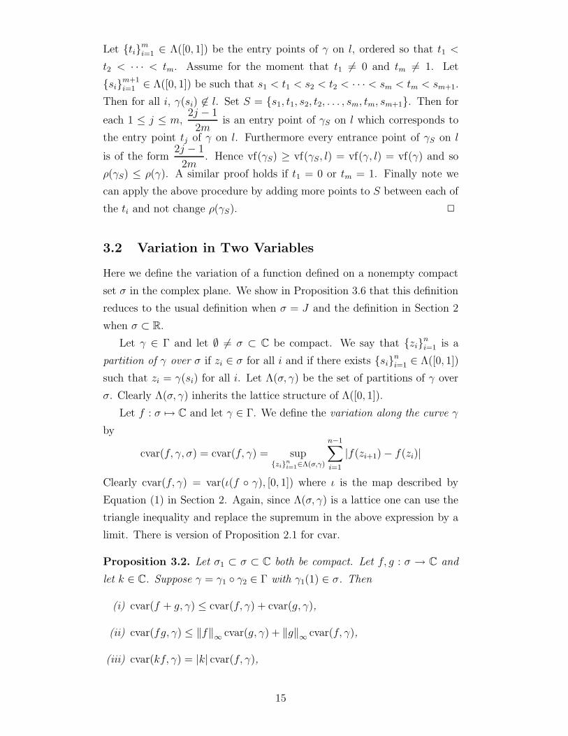
or for γ ∈ C([a, b]) rather than γ ∈ C([0, 1]). Figure 1 illustrates a curve
γ ∈ Γ with four entry points t1, t2, t3 and t4 on a line l.
Suppose γ ∈ Γ and {γi}ni=1 ⊂ Γ. Set vf(γ, l) to be the number of entry
points of γ on l and set vf(∪ni=1γi, l) =
n∑
i=1
vf(γi, l). Clearly if γ1∼= γ2 then
vf(γ1, l) = vf(γ2, l). We set vf(γ) and vf(∪ni=1γi) to be the supremum of
vf(γ, l) and vf(∪ni=1γi, l) over all lines l. We write vfH(γ) for the supremum
of vf(γ, l) over all horizontal lines l, vfV for the supremum of vf(γ, l) over
all vertical lines, and so on. Clearly vf ≥ vfH and vf ≥ vfV. We write ρ
for1
vf. For example ρV(∪n
i=1γi) =1
vfV(∪ni=1γi)
. If, for example, vf(γ) = ∞then we take the convention that ρ(γ) = 0. It is also clear that ρ ≤ ρH,
ρ ≤ ρV and that if γ1∼= γ2 then ρ(γ1) = ρ(γ2). We can extend the notion
of ρ, ρV and so on to include curves in C([a, b]) in the obvious way.
In Figure 2 there are three curves γ1, γ2, γ3 ∈ Γ. From the diagram one
can see that vf(∪3i=1γi, l) = 6. No line has more entry points on each curve
than does l. Hence ρ(γ1) = 1, ρ(γ2) =1
2and ρ(γ3) =
1
3. It is easy to see
that ρH(γi) = ρ(γi) for each i and that ρV(γ1) = ρV(γ3) = 1 and ρV(γ2) =1
2.
Let σ ⊂ C be compact and let l be a line parameterized by R. Then
t ∈ R is said to be an entry point of l on σ if l(t) ∈ σ and for all ε > 0 there
exists s ∈ (t − ε, t) such that l(s) 6∈ σ. Again set vf(σ, l) to be the number
of entry points of l on σ and vf(σ) to be the supremum of vf(σ, l) over all
lines l. Clearly vf(σ, l) does not depend on the choice of parameterization
of the line l.
Note that if γ ∈ Γ then it does not follow that vf(γ) = vf(γ([0, 1])). For
example if γ is given by
γ(t) =
2t if 0 ≤ t ≤ 1
2,
2 − 2t if1
2< t ≤ 1.
12

PSfrag replacements
l
γ
t1 t2 t3 t4
Figure 1: Entry points t1, . . . , t4 of γ along l.
PSfrag replacements
l
γ1 γ2 γ3
Figure 2: ρ(γ1) = 1, ρ(γ2) =1
2and ρ(γ3) =
1
3.
13
Then vf(γ([0, 1])) = vf([0, 1]) = 1 but vf(γ) = vf(γ, R) = 2.
We now define a set of curves ΓL which we later show allows us to
approximate any γ ∈ Γ by a curve consisting of line segments. Let j, n ∈ Z+
and suppose that j < n. For t ∈[
j − 1
n − 1,
j
n − 1
]
define
αj,n(t) = (n − 1)t − (j − 1).
Hence αj,n maps
[
j − 1
n − 1,
j
n − 1
]
homeomorphically onto [0, 1]. Let z1, . . . , zn ∈C. Write Π(z1, z2, . . . , zn) for the function [0, 1] → C defined on each inter-
val
[
j − 1
n − 1,
j
n − 1
]
for 1 ≤ j ≤ n − 1 by
Π(z1, z2, . . . , zn)(t) = (1 − αj,n(t))zj + αj,n(t)zj+1.
Hence Π(z1, z2, . . . , zn) ∈ Γ and is a curve consisting of line segments, whose
endpoints are z1, z2, . . . zn and which is parameterized by [0, 1].
Set
ΓL = {γ ∈ Γ : γ ∼= Π(z1, z2, . . . , zn) for some zi ∈ C and n ∈ N} .
Let γ ∈ Γ. Let S = {si}ni=1 ∈ Λ([0, 1]). Set
γS = Π(γ(s1), γ(s2), . . . , γ(sn)) ∈ ΓL.
The curve γS is said to be the S approximation of γ.
Lemma 3.1. Let γ ∈ Γ and suppose vf(γ) < ∞. Then limS∈Λ([0,1])
ρ(γS) =
ρ(γ).
Proof. Fix S = {si}ni=1 ∈ Λ([0, 1]). Let l be a line. If t ∈ [0, 1] is an entry
point of γS on l then there exist 1 ≤ j ≤ n−1 such that t ∈[
j − 1
n − 1,
j
n − 1
]
.
Since l is a line and γS
([
j − 1
n − 1,
j
n − 1
])
is a line segment then there is
no other entry point t′ of γS on l such that t′ ∈[
j − 1
n − 1,
j
n − 1
]
. But since
γ is continuous, γ(sj) = γS
(
j − 1
n − 1
)
and γ(sj+1) = γS
(
j
n − 1
)
it follows
there is at least one entry point s of γ on l such that sj ≤ s ≤ sj+1. Hence
vf(γS, l) ≤ vf(γ, l) and so ρ(γS) ≥ ρ(γ).
To conclude the proof we show that there exists S ∈ Λ([0, 1]) such
that ρ(γS) ≤ ρ(γ) and that for any refinement S ′ of S, ρ(γS′) ≤ ρ(γ).
Since vf(γ) < ∞ there exists a line l such that vf(γ, l) = vf(γ) := m.
14
Let {ti}m
i=1 ∈ Λ([0, 1]) be the entry points of γ on l, ordered so that t1 <
t2 < · · · < tm. Assume for the moment that t1 6= 0 and tm 6= 1. Let
{si}m+1i=1 ∈ Λ([0, 1]) be such that s1 < t1 < s2 < t2 < · · · < sm < tm < sm+1.
Then for all i, γ(si) 6∈ l. Set S = {s1, t1, s2, t2, . . . , sm, tm, sm+1}. Then for
each 1 ≤ j ≤ m,2j − 1
2mis an entry point of γS on l which corresponds to
the entry point tj of γ on l. Furthermore every entrance point of γS on l
is of the form2j − 1
2m. Hence vf(γS) ≥ vf(γS, l) = vf(γ, l) = vf(γ) and so
ρ(γS) ≤ ρ(γ). A similar proof holds if t1 = 0 or tm = 1. Finally note we
can apply the above procedure by adding more points to S between each of
the ti and not change ρ(γS). 2
3.2 Variation in Two Variables
Here we define the variation of a function defined on a nonempty compact
set σ in the complex plane. We show in Proposition 3.6 that this definition
reduces to the usual definition when σ = J and the definition in Section 2
when σ ⊂ R.
Let γ ∈ Γ and let ∅ 6= σ ⊂ C be compact. We say that {zi}ni=1 is a
partition of γ over σ if zi ∈ σ for all i and if there exists {si}n
i=1 ∈ Λ([0, 1])
such that zi = γ(si) for all i. Let Λ(σ, γ) be the set of partitions of γ over
σ. Clearly Λ(σ, γ) inherits the lattice structure of Λ([0, 1]).
Let f : σ 7→ C and let γ ∈ Γ. We define the variation along the curve γ
by
cvar(f, γ, σ) = cvar(f, γ) = sup{zi}
ni=1∈Λ(σ,γ)
n−1∑
i=1
|f(zi+1) − f(zi)|
Clearly cvar(f, γ) = var(ι(f ◦ γ), [0, 1]) where ι is the map described by
Equation (1) in Section 2. Again, since Λ(σ, γ) is a lattice one can use the
triangle inequality and replace the supremum in the above expression by a
limit. There is version of Proposition 2.1 for cvar.
Proposition 3.2. Let σ1 ⊂ σ ⊂ C both be compact. Let f, g : σ → C and
let k ∈ C. Suppose γ = γ1 ◦ γ2 ∈ Γ with γ1(1) ∈ σ. Then
(i) cvar(f + g, γ) ≤ cvar(f, γ) + cvar(g, γ),
(ii) cvar(fg, γ) ≤ ‖f‖∞ cvar(g, γ) + ‖g‖∞ cvar(f, γ),
(iii) cvar(kf, γ) = |k| cvar(f, γ),
15

(iv) cvar(f, γ) = cvar(f, γ1) + cvar(f, γ2),
(v) cvar(f, γ1) ≤ cvar(f, γ),
(vi) cvar(f, γ, σ1) ≤ cvar(f, γ, σ).
Proof. The proofs are the same as for Proposition 2.1. 2
Note that the variation along a curve does not depend on the parame-
terization.
Lemma 3.3. Let f : σ → C. Let γ1, γ2 ∈ Γ and suppose that γ1∼= γ2.
Then cvar(f, γ1) = cvar(f, γ2).
Definition 3.4. Let f : σ → C. Then variation of f on σ is defined to be
var(f, σ) = supγ∈Γ
ρ(γ) cvar(f, γ). (2)
Here we take the convention that if γ ∈ Γ is such that ρ(γ) = 0 and if
cvar(f, γ) = ∞ then ρ(γ) cvar(f, γ) = 0. As we shall show in Proposition
3.6 this notation is not ambiguous since it agrees with the notation given
in Section 2 if σ ⊂ R.
In practice, Γ is usually too large a set to work with. As the next lemma
shows, one can replace Γ with ΓL (or indeed any of a number of sets of
simpler curves) and obtain the same definition of variation over σ.
Lemma 3.5. Let f : σ → C. Then
supγ∈ΓL
ρ(γ) cvar(f, γ) = supγ∈Γ
ρ(γ) cvar(f, γ).
Proof. Clearly supγ∈ΓL
ρ(γ) cvar(f, γ) ≤ supγ∈Γ
ρ(γ) cvar(f, γ). Let γ ∈ Γ. We
may assume that ρ(γ) > 0. Let S = {si}ni=1 ∈ Λ(σ, γ). Then
n−1∑
i=1
|f(si+1) − f(si)| ≤
cvar(f, γS). Then by Lemma 3.1
ρ(γ) cvar(f, γ) = limS={si}
ni=1
∈Λ(σ,γ)ρ(γ)
n−1∑
i=1
|f(si+1) − f(si)|
≤ limS∈Λ(σ,γ)
ρ(γ) cvar(f, γS)
= limS∈Λ(σ,γ)
ρ(γS) cvar(f, γS)
≤ supγ′∈ΓL
ρ(γ′) cvar(f, γ′).
2
16
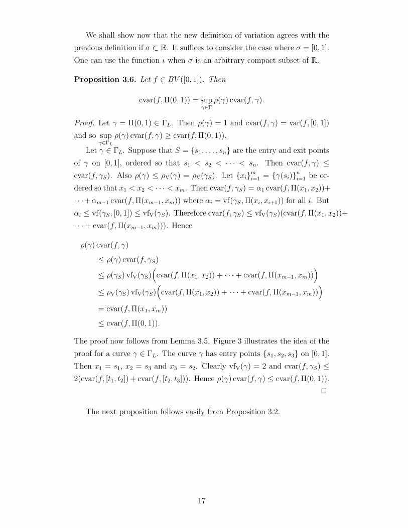
We shall show now that the new definition of variation agrees with the
previous definition if σ ⊂ R. It suffices to consider the case where σ = [0, 1].
One can use the function ι when σ is an arbitrary compact subset of R.
Proposition 3.6. Let f ∈ BV ([0, 1]). Then
cvar(f, Π(0, 1)) = supγ∈Γ
ρ(γ) cvar(f, γ).
Proof. Let γ = Π(0, 1) ∈ ΓL. Then ρ(γ) = 1 and cvar(f, γ) = var(f, [0, 1])
and so supγ∈ΓL
ρ(γ) cvar(f, γ) ≥ cvar(f, Π(0, 1)).
Let γ ∈ ΓL. Suppose that S = {s1, . . . , sn} are the entry and exit points
of γ on [0, 1], ordered so that s1 < s2 < · · · < sn. Then cvar(f, γ) ≤cvar(f, γS). Also ρ(γ) ≤ ρV(γ) = ρV(γS). Let {xi}m
i=1 = {γ(si)}ni=1 be or-
dered so that x1 < x2 < · · · < xm. Then cvar(f, γS) = α1 cvar(f, Π(x1, x2))+
· · ·+αm−1 cvar(f, Π(xm−1, xm)) where αi = vf(γS, Π(xi, xi+1)) for all i. But
αi ≤ vf(γS, [0, 1]) ≤ vfV(γS). Therefore cvar(f, γS) ≤ vfV(γS)(cvar(f, Π(x1, x2))+
· · ·+ cvar(f, Π(xm−1, xm))). Hence
ρ(γ) cvar(f, γ)
≤ ρ(γ) cvar(f, γS)
≤ ρ(γS) vfV(γS)(
cvar(f, Π(x1, x2)) + · · · + cvar(f, Π(xm−1, xm)))
≤ ρV(γS) vfV(γS)(
cvar(f, Π(x1, x2)) + · · · + cvar(f, Π(xm−1, xm)))
= cvar(f, Π(x1, xm))
≤ cvar(f, Π(0, 1)).
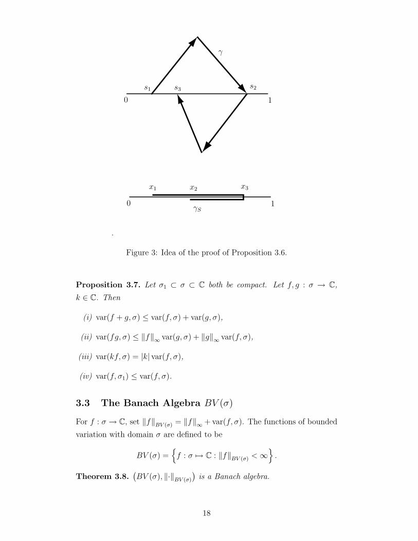
The proof now follows from Lemma 3.5. Figure 3 illustrates the idea of the
proof for a curve γ ∈ ΓL. The curve γ has entry points {s1, s2, s3} on [0, 1].
Then x1 = s1, x2 = s3 and x3 = s2. Clearly vfV(γ) = 2 and cvar(f, γS) ≤2(cvar(f, [t1, t2]) + cvar(f, [t2, t3])). Hence ρ(γ) cvar(f, γ) ≤ cvar(f, Π(0, 1)).
2
The next proposition follows easily from Proposition 3.2.
17
.
PSfrag replacements
0
0
1
1
s1 s2s3
γ
x1 x2 x3
γS
Figure 3: Idea of the proof of Proposition 3.6.
Proposition 3.7. Let σ1 ⊂ σ ⊂ C both be compact. Let f, g : σ → C,
k ∈ C. Then
(i) var(f + g, σ) ≤ var(f, σ) + var(g, σ),
(ii) var(fg, σ) ≤ ‖f‖∞ var(g, σ) + ‖g‖∞ var(f, σ),
(iii) var(kf, σ) = |k| var(f, σ),
(iv) var(f, σ1) ≤ var(f, σ).
3.3 The Banach Algebra BV (σ)
For f : σ → C, set ‖f‖BV (σ) = ‖f‖∞ + var(f, σ). The functions of bounded
variation with domain σ are defined to be
BV (σ) ={
f : σ 7→ C : ‖f‖BV (σ) < ∞}
.
Theorem 3.8.(
BV (σ), ‖·‖BV (σ)
)
is a Banach algebra.
18
Proof. Checking that ‖·‖BV (σ) satisfies the properties of an algebra norm is
straightforward. For example using Proposition 3.7 we have
‖fg‖BV (σ) = ‖fg‖∞ + var(fg, γ)
≤ ‖f‖∞ ‖g‖∞ + ‖f‖∞ var(g, σ) + ‖g‖∞ var(f, σ)
≤ ‖f‖∞ ‖g‖∞ + ‖f‖∞ var(g, σ) + ‖g‖∞ var(f, σ)
+ var(f, σ) var(g, σ)
=(
‖f‖∞ + var(f, σ))(
‖g‖∞ + var(g, σ))
= ‖f‖BV (σ) ‖g‖BV (σ) .
It remains to show that BV (σ) is complete. Let {fn}∞n=1 be a Cauchy
sequence in BV (σ). Fix ε > 0. By the definition of ‖·‖BV (σ), {fn}∞n=1
converges uniformly to a function f . Choose N1 so that n ≥ N1 implies
‖f − fn‖∞ <ε
2. Being a Cauchy sequence in BV (σ) means there exists an
N2 so that m, n > N2 implies for all γ ∈ Γ and all {zi}ni=1 ∈ Λ(σ, γ) we have
that
ρ(γ)n−1∑
i=1
|(fn − fm)(zi+1) − (fn − fm)(zi)| <ε
2.
Let N = max {N1, N2}. Let n > N , let γ ∈ Γ and let {zi}ni=1 ∈ Λ(σ, γ).
Then
ρ(γ)
n−1∑
i=1
|(fn − f)(zi+1) − (fn − f)(zi)|
= limm
ρ(γ)
n−1∑
i=1
|(fn − fm)(zi+1) − (fn − fm)(zi)|
<ε
2.
Hence
var(f − fn, σ) = supγ∈ΓL
ρ(γ) cvar(f − fn, γ)
= supγ∈ΓL
sup{zi}
ni=1∈Λ(σ,γ)
ρ(γ)
n−1∑
i=1
|(fn − f)(zi+1) − (fn − f)(zi)|
≤ ε
2.
Finally ‖f − fn‖BV (σ) = ‖f − fn‖∞ + var(f − fn, σ) ≤ ε
2+
ε
2= ε. 2
These algebras respect domain inclusion in the expected manner.
19
Lemma 3.9. Suppose that σ1 ⊂ σ2 ⊂ C are both compact and that f ∈BV (σ2). Then ‖f |σ1‖BV (σ1) ≤ ‖f‖BV (σ2) and so f |σ1 ∈ BV (σ1).
Proof. By Proposition 3.7 (iv)
‖f |σ1‖BV (σ1) = ‖f |σ1‖∞ + var(f |σ1, σ1)
≤ ‖f‖∞ + var(f, σ2)
= ‖f‖BV (σ2) .
2
3.4 Affine Invariance
One of the objectives in this paper was to have an algebra which has the
same sort of affine invariance properties as C(σ). Let f ∈ BV (σ). Define
θα,β(f) : ασ + β → C by
θα,β(f)(z) = f(α−1(z − β)).
Proposition 3.10. For any α, β ∈ C, α 6= 0, the map θα,β is an isometric
isomorphism from BV (σ) onto BV (ασ + β).
Proof. Clearly θα,β is a linear homomorphism. Let f ∈ BV (σ) and let
γ ∈ Γ. Then αγ + β ∈ Γ. Hence
cvar(f, γ, σ) = sup{zi}
ni=1
∈Λ(σ,γ)
n−1∑
i=1
|f(zi+1) − f(zi)|
= sup{wi}
ni=1
∈Λ(ασ+β,αγ+β)
n−1∑
i=1
∣
∣f(α−1(wi+1 − β)) − f(α−1(wi − β))∣
∣
= sup{wi}
ni=1∈Λ(ασ+β,αγ+β)
n−1∑
i=1
|θα,β(f)(wi+1) − θα,β(f)(wi)|
= cvar(θα,β(f), αγ + β, ασ + β).
Since ρ(γ) = ρ(αγ + β) it follows that var(θα,β(f), ασ + β) = var(f, σ).
It is clear that ‖θα,β(f)‖∞ = ‖f‖∞. Hence ‖θα,β(f)‖BV (ασ+β) = ‖f‖BV (σ).
Finally note that (θα,β)−1 = θα−1,−α−1β. 2
3.5 Compositions of functions
It is possible to generalize Proposition 3.6 to the following proposition. This
result allows us to conclude that many important AC operators (such as
20
the trigonometrically well-bounded operators) are also AC(σ) operators for
some σ.
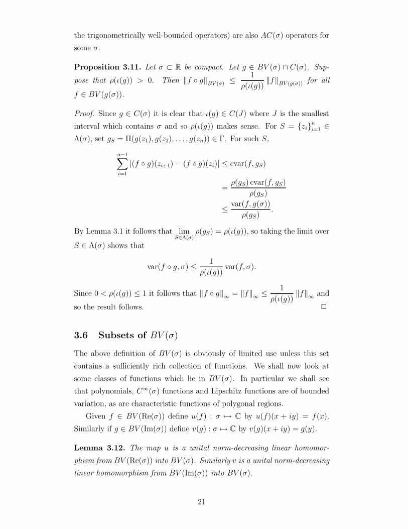
Proposition 3.11. Let σ ⊂ R be compact. Let g ∈ BV (σ) ∩ C(σ). Sup-
pose that ρ(ι(g)) > 0. Then ‖f ◦ g‖BV (σ) ≤ 1
ρ(ι(g))‖f‖BV (g(σ)) for all
f ∈ BV (g(σ)).
Proof. Since g ∈ C(σ) it is clear that ι(g) ∈ C(J) where J is the smallest
interval which contains σ and so ρ(ι(g)) makes sense. For S = {zi}n
i=1 ∈Λ(σ), set gS = Π(g(z1), g(z2), . . . , g(zn)) ∈ Γ. For such S,
n−1∑
i=1
|(f ◦ g)(zi+1) − (f ◦ g)(zi)| ≤ cvar(f, gS)
=ρ(gS) cvar(f, gS)
ρ(gS)
≤ var(f, g(σ))
ρ(gS).
By Lemma 3.1 it follows that limS∈Λ(σ)
ρ(gS) = ρ(ι(g)), so taking the limit over
S ∈ Λ(σ) shows that
var(f ◦ g, σ) ≤ 1
ρ(ι(g))var(f, σ).
Since 0 < ρ(ι(g)) ≤ 1 it follows that ‖f ◦ g‖∞ = ‖f‖∞ ≤ 1
ρ(ι(g))‖f‖∞ and
so the result follows. 2
3.6 Subsets of BV (σ)
The above definition of BV (σ) is obviously of limited use unless this set
contains a sufficiently rich collection of functions. We shall now look at
some classes of functions which lie in BV (σ). In particular we shall see
that polynomials, C∞(σ) functions and Lipschitz functions are of bounded
variation, as are characteristic functions of polygonal regions.
Given f ∈ BV (Re(σ)) define u(f) : σ 7→ C by u(f)(x + iy) = f(x).
Similarly if g ∈ BV (Im(σ)) define v(g) : σ 7→ C by v(g)(x + iy) = g(y).
Lemma 3.12. The map u is a unital norm-decreasing linear homomor-
phism from BV (Re(σ)) into BV (σ). Similarly v is a unital norm-decreasing
linear homomorphism from BV (Im(σ)) into BV (σ).
21

Proof. The only thing not clear is that u and v are norm-decreasing. Let
f ∈ BV (Re(σ)) and let γ ∈ ΓL. Recall that Re(γ) is defined by Re(γ)(t) =
Re(γ(t)). Clearly Re(γ) ∈ ΓL. From |u(f)(t) − u(f)(s)| = |f(Re(t)) − f(Re(s))|it follows that cvar(u(f), γ, σ) = cvar(f, Re(γ), Re(σ)). Also, using a similar
argument to that used in Proposition 3.6, we have that cvar(f, Re(γ), Re(σ)) ≤vfV(γ) var(f, Re(γ)). Then
ρ(γ) cvar(u(f), γ, σ) = ρ(γ) cvar(f, Re(γ), Re(σ))
≤ ρV(γ) cvar(f, Re(γ), Re(σ))
≤ ρV(γ) vfV(γ) var(f, Re(γ))
= var(f, Re(γ))
≤ var(f, Re(σ)).
Taking the supremum over all γ ∈ ΓL and using Lemma 3.5 gives the result.
The proof for v is very similar. 2
To show that all the polynomials are in BV (σ), it suffices to show that
the function λσ : σ → C, λσ(z) = z lies in BV (σ). Where there is little
chance of confusion we shall write λ rather than λσ. Let P2 denote the
polynomials in z and z.
Corollary 3.13. λ, λ ∈ BV (σ).
Proof. λ = u(
λRe(σ)
)
+ iv(
λIm(σ)
)
. 2
Corollary 3.14. P2 ⊂ BV (σ).
Given a compact set σ ⊂ C let
Cσ = var(λ, σ).
Given γ = Π(z1, z2, . . . , zn) ∈ ΓL we write l(γ) for the length of γ. That is
l(γ) =
n−1∑
i=1
|zi+1 − zi|. Then l(γ) = cvar(λ, γ) and so ρ(γ)l(γ) ≤ Cσ. Since σ
is compact there exists z, w ∈ σ such that diam(σ) = |z − w|. In this case
diam(σ) = |z − w| = cvar(λ, Π(z, w)) ≤ var(λ, σ). In general this inequality
is strict. For example let σ = [0, 1]×[0, 1]. If γ = Π(0, 1, 1+i, i, 0) ∈ ΓL then
ρ(γ) =1
2and cvar(λ, γ) = 4. Hence diam(σ) =
√2 < 2 = ρ(γ) cvar(λ, γ) ≤
var(λ, σ).
Recall that we write Lip(σ) for the Lipschitz functions with domain σ
and L(f) for the Lipschitz constant of f ∈ Lip(σ).
22
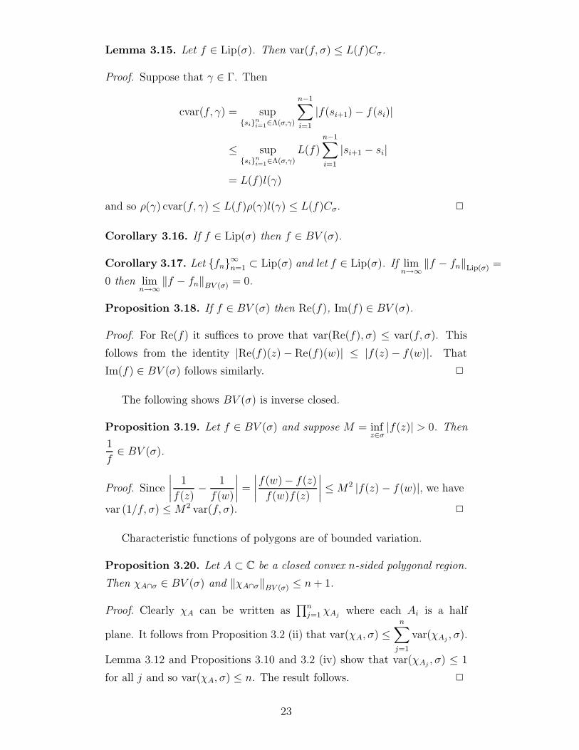
Lemma 3.15. Let f ∈ Lip(σ). Then var(f, σ) ≤ L(f)Cσ.
Proof. Suppose that γ ∈ Γ. Then
cvar(f, γ) = sup{si}
ni=1
∈Λ(σ,γ)
n−1∑
i=1
|f(si+1) − f(si)|
≤ sup{si}
ni=1
∈Λ(σ,γ)
L(f)n−1∑
i=1
|si+1 − si|
= L(f)l(γ)
and so ρ(γ) cvar(f, γ) ≤ L(f)ρ(γ)l(γ) ≤ L(f)Cσ. 2
Corollary 3.16. If f ∈ Lip(σ) then f ∈ BV (σ).
Corollary 3.17. Let {fn}∞n=1 ⊂ Lip(σ) and let f ∈ Lip(σ). If limn→∞
‖f − fn‖Lip(σ) =
0 then limn→∞
‖f − fn‖BV (σ) = 0.
Proposition 3.18. If f ∈ BV (σ) then Re(f), Im(f) ∈ BV (σ).
Proof. For Re(f) it suffices to prove that var(Re(f), σ) ≤ var(f, σ). This
follows from the identity |Re(f)(z) − Re(f)(w)| ≤ |f(z) − f(w)|. That
Im(f) ∈ BV (σ) follows similarly. 2
The following shows BV (σ) is inverse closed.
Proposition 3.19. Let f ∈ BV (σ) and suppose M = infz∈σ
|f(z)| > 0. Then
1
f∈ BV (σ).
Proof. Since
∣
∣
∣
∣
1
f(z)− 1
f(w)
∣
∣
∣
∣
=
∣
∣
∣
∣
f(w) − f(z)
f(w)f(z)
∣
∣
∣
∣
≤ M2 |f(z) − f(w)|, we have
var (1/f, σ) ≤ M 2 var(f, σ). 2
Characteristic functions of polygons are of bounded variation.
Proposition 3.20. Let A ⊂ C be a closed convex n-sided polygonal region.
Then χA∩σ ∈ BV (σ) and ‖χA∩σ‖BV (σ) ≤ n + 1.
Proof. Clearly χA can be written as∏n
j=1 χAjwhere each Ai is a half
plane. It follows from Proposition 3.2 (ii) that var(χA, σ) ≤n∑
j=1
var(χAj, σ).
Lemma 3.12 and Propositions 3.10 and 3.2 (iv) show that var(χAj, σ) ≤ 1
for all j and so var(χA, σ) ≤ n. The result follows. 2
23

There is, just as in the one variable case, a severe restriction on the form
of idempotent functions in BV (σ). It is not too hard to show that if the
polygon A sits within the interior of σ then the above estimate is sharp.
Indeed, sets formed by taking a finite number of set operations involving
polygons are essentially the only sets whose characteristic functions are in
BV (σ). Making this precise is slightly delicate, since what really matters
is how the set A intersects with σ. These questions will be pursued in more
detail in [3].
If σ = J ×K is a rectangle (with sides parallel to the axes), it is natural
to ask how this new definition compares to the more classical notion (due
to Hardy and Krause) which was used by Berkson and Gillespie in their
definition of AC-operators [7]. We shall denote by BVHK(J×K) the Banach
algebra of functions on J ×K which are of bounded variation in the Hardy-
Krause sense. We show in [4] that
(i) BVHK(J × K) ⊂ BV (J × K).
(ii) The inclusion map BVHK(J × K) ↪→ BV (J × K) is continuous.
(iii) If J and K are nondegenerate, then BVHK(J × K) 6= BV (J × K).
4 AC(σ) for σ ⊂ C Compact
From an operator theoretic point of view, one would like to be able to
deduce structural information about an operator T from bounds on ‖p(T )‖for p in some small algebra of functions. In the case that X is reflexive and
σ(T ) ⊂ R, then a bound of the form ‖p(T )‖ ≤ C ‖p‖∞ is sufficient to show
that T can be written as an integral with respect to a countably additive
spectral measure, whereas a weaker bound of the form ‖p(T )‖ ≤ C ‖p‖AC
implies that T has an integral representation with respect to a spectral
family of projections. If the spectrum is not real then it is unrealistic to
expect to be able to prove much unless the algebra contains at least P2, the
polynomials in two variables. This leads to our definition of the absolutely
continuous functions defined on a non-empty compact subset σ of C. These
form a Banach subalgebra AC(σ) of BV (σ). In this section we look at some
classes of functions in AC(σ). We show, for example, that C∞(σ) ⊂ AC(σ).
Rather surprisingly however, Example 4.13 shows that unlike the situation
when σ ⊂ R, Lipschitz functions are not necessarily absolutely continuous.
24
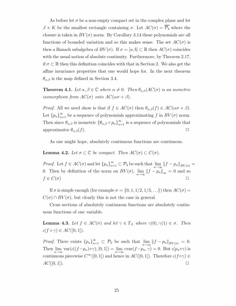
As before let σ be a non-empty compact set in the complex plane and let
J × K be the smallest rectangle containing σ. Let AC(σ) = P2 where the
closure is taken in BV (σ) norm. By Corollary 3.14 these polynomials are all
functions of bounded variation and so this makes sense. The set AC(σ) is
then a Banach subalgebra of BV (σ). If σ = [a, b] ⊂ R then AC(σ) coincides
with the usual notion of absolute continuity. Furthermore, by Theorem 2.17,
if σ ⊂ R then this definition coincides with that in Section 2. We also get the
affine invariance properties that one would hope for. In the next theorem
θα,β is the map defined in Section 3.4.
Theorem 4.1. Let α, β ∈ C where α 6= 0. Then θα,β|AC(σ) is an isometric
isomorphism from AC(σ) onto AC(ασ + β).
Proof. All we need show is that if f ∈ AC(σ) then θα,β(f) ∈ AC(ασ + β).
Let {pn}∞n=1 be a sequence of polynomials approximating f in BV (σ) norm.
Then since θα,β is isometric {θα,β ◦ pn}∞n=1 is a sequence of polynomials that
approximates θα,β(f). 2
As one might hope, absolutely continuous functions are continuous.
Lemma 4.2. Let σ ⊂ C be compact. Then AC(σ) ⊂ C(σ).
Proof. Let f ∈ AC(σ) and let {pn}∞n=1 ⊂ P2 be such that limn→∞
‖f − pn‖BV (σ) =
0. Then by definition of the norm on BV (σ), limn→∞
‖f − pn‖∞ = 0 and so
f ∈ C(σ) 2
If σ is simple enough (for example σ = {0, 1, 1/2, 1/3, . . .}) then AC(σ) =
C(σ) ∩ BV (σ), but clearly this is not the case in general.
Cross sections of absolutely continuous functions are absolutely contin-
uous functions of one variable.
Lemma 4.3. Let f ∈ AC(σ) and let γ ∈ ΓL where γ(0), γ(1) ∈ σ. Then
ι(f ◦ γ) ∈ AC([0, 1]).
Proof. There exists {pn}∞n=1 ⊂ P2 be such that limn→∞
‖f − pn‖BV (σ) = 0.
Then limn→∞
var(ι((f−pn)◦γ), [0, 1]) = limn→∞
cvar(f−pn, γ) = 0. But ι(pn◦γ) is
continuous piecewise C∞([0, 1]) and hence in AC([0, 1]). Therefore ι(f ◦γ) ∈AC([0, 1]). 2
25
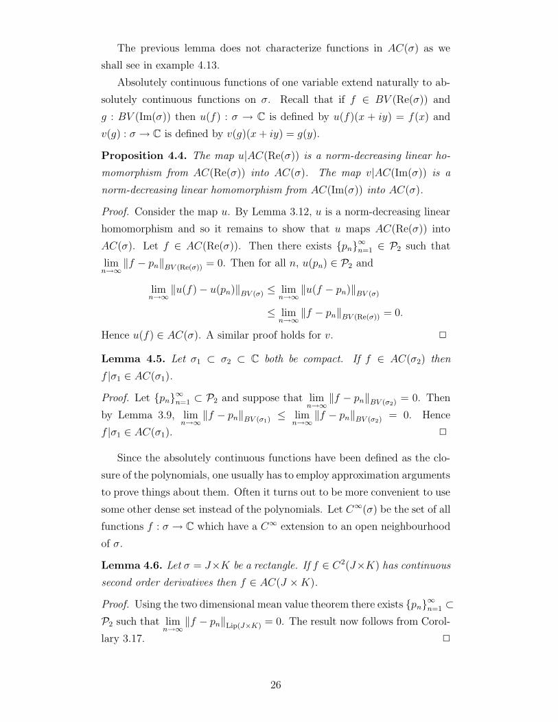
The previous lemma does not characterize functions in AC(σ) as we
shall see in example 4.13.
Absolutely continuous functions of one variable extend naturally to ab-
solutely continuous functions on σ. Recall that if f ∈ BV (Re(σ)) and
g : BV (Im(σ)) then u(f) : σ → C is defined by u(f)(x + iy) = f(x) and
v(g) : σ → C is defined by v(g)(x + iy) = g(y).
Proposition 4.4. The map u|AC(Re(σ)) is a norm-decreasing linear ho-
momorphism from AC(Re(σ)) into AC(σ). The map v|AC(Im(σ)) is a
norm-decreasing linear homomorphism from AC(Im(σ)) into AC(σ).
Proof. Consider the map u. By Lemma 3.12, u is a norm-decreasing linear
homomorphism and so it remains to show that u maps AC(Re(σ)) into
AC(σ). Let f ∈ AC(Re(σ)). Then there exists {pn}∞n=1 ∈ P2 such that
limn→∞
‖f − pn‖BV (Re(σ)) = 0. Then for all n, u(pn) ∈ P2 and
limn→∞
‖u(f) − u(pn)‖BV (σ) ≤ limn→∞
‖u(f − pn)‖BV (σ)
≤ limn→∞
‖f − pn‖BV (Re(σ)) = 0.
Hence u(f) ∈ AC(σ). A similar proof holds for v. 2
Lemma 4.5. Let σ1 ⊂ σ2 ⊂ C both be compact. If f ∈ AC(σ2) then
f |σ1 ∈ AC(σ1).
Proof. Let {pn}∞n=1 ⊂ P2 and suppose that limn→∞
‖f − pn‖BV (σ2) = 0. Then
by Lemma 3.9, limn→∞
‖f − pn‖BV (σ1) ≤ limn→∞
‖f − pn‖BV (σ2) = 0. Hence
f |σ1 ∈ AC(σ1). 2
Since the absolutely continuous functions have been defined as the clo-
sure of the polynomials, one usually has to employ approximation arguments
to prove things about them. Often it turns out to be more convenient to use
some other dense set instead of the polynomials. Let C∞(σ) be the set of all
functions f : σ → C which have a C∞ extension to an open neighbourhood
of σ.
Lemma 4.6. Let σ = J×K be a rectangle. If f ∈ C2(J×K) has continuous
second order derivatives then f ∈ AC(J × K).
Proof. Using the two dimensional mean value theorem there exists {pn}∞n=1 ⊂P2 such that lim
n→∞‖f − pn‖Lip(J×K) = 0. The result now follows from Corol-
lary 3.17. 2
26

Proposition 4.7. C∞(σ) is a dense subset of AC(σ).
Proof. Let f ∈ C∞(σ). By definition there exists F ∈ C∞(U), an extension
of f defined on an open neighbourhood U of σ. We can then choose V open
with minimally smooth boundary (see [16, Section 6.3.3]) and σ ⊂ V ⊂ U .
Then F |V can be extended to a function, also denoted F , in C∞(J × K).
Hence by Lemma 4.6, F ∈ AC(J × K) and so by Lemma 4.5, f = F |σ ∈AC(σ). The density follows from the fact that polynomials are in C∞(σ).
2
Proposition 4.7 allows simple proofs that absolutely continuous functions
are stable under simple operations.
Corollary 4.8. If f ∈ AC(σ) then Re(f), Im(f) ∈ AC(σ).
Proof. Let {pn}∞n=1 be a sequence of polynomials such that limn→∞
‖f − pn‖BV (σ) =
0. Then {Re(pn)}∞n=1 ⊂ C∞(σ). By Proposition 3.18, limn→∞
‖Re(f) − Re(pn)‖BV (σ) ≤lim
n→∞‖f − pn‖BV (σ) = 0. Hence Re(f) ∈ AC(σ). Similarly Im(f) ∈ AC(σ).
2
Corollary 4.9. If f ∈ AC(σ) and f(z) 6= 0 on σ then1
f∈ AC(σ).
Proof. Let {pn}∞n=1 be a sequence of polynomials approximating f in BV (σ)
norm. Let M = infz∈σ
|f(z)| and Mn = infz∈σ
|f(z)pn(z)|. Since σ is closed and
f is continuous it follows that M > 0. Clearly limn→∞
Mn = M2. For large
enough n,1
pn
∈ C∞(σ). Then limn→∞
∥
∥
∥
∥
1
fpn
∥
∥
∥
∥
∞
= limn→∞
M−1n = M−2. Also, by
Proposition 3.19,
limn→∞
var
(
1
fpn
, σ
)
≤ limn→∞
M2n var(pnf, σ)
= M4 var(f 2, σ) < ∞.
Then
limn→∞
var
(
1
f− 1
pn
, σ
)
= limn→∞
var
(
pn − f
pnf, σ
)
≤ limn→∞
var(pn − f, σ)
∥
∥
∥
∥
1
pnf
∥
∥
∥
∥
∞
+ limn→∞
var
(
1
pnf, σ
)
‖pn − f‖∞
= 0.
2
27

In some cases it is more convenient to work with an appropriate ana-
logue of continuous piecewise linear functions. We shall now define such an
analogue and prove that this class of functions is always dense in AC(σ).
We say that a finite partition {Ai}ni=1 is a triangulation of a rectangle J×K
if
(i) for each i, Ai is a non-degenerate (topologically) closed triangle,
(ii) for all i, j where i 6= j, int(Ai) ∩ int(Aj) = ∅,
(iii) ∪ni=1Ai = J × K.
A function F : J×K → C is said to be continuous and piecewise triangularly
planar if F is continuous and there is a triangulation {Ai}ni=1 such that for
each i, F |Ai is planar. The set of continuous piecewise triangularly planar
functions with domain J × K is denoted CTPP (J × K). It is easy to see
that if F, G ∈ CTPP (J ×K) then there exists a triangulation {Ai}n
i=1 such
that F + G|Ai is planar for all i. Hence CTPP (J × K) is a vector space.
Lemma 4.10. The set CTPP (J × K) is dense in AC(J × K).
Proof. This follows from the two-dimensional mean value theorem. In par-
ticular we can always approximate in Lipschitz norm any polynomial by a
continuous piecewise planar function and hence approximate in BV (J ×K)
norm. 2
We say that A ⊂ σ is a triangle relative to σ if there exists A′ ⊂ J × K
such that A′ is a topologically closed triangle and if A = A′ ∩ σ. We
say {Ai}n
i=1 is a triangulation of σ if Ai ⊂ σ for all i and there exists a
triangulation {A′i}
m
i=1 of J ×K such that Ai = A′i ∩ σ for all 1 ≤ i ≤ n. We
say a function f is continuous and piecewise triangularly planar relative to
σ if f is continuous and there is some triangulation {Ai}ni=1 of σ such that
f |Ai is planar for all i. The set of continuous and piecewise triangularly
planar functions relative to σ is denoted CTPP (σ). This agrees with the
previous definition of σ = J ×K. Clearly f ∈ CTPP (σ) if and only if there
exists F ∈ CTPP (J × K) such that F |σ = f .
Lemma 4.11. The set CTPP (σ) is dense in AC(σ).
Proof. Suppose that f ∈ AC(σ) and ε > 0. Then there exists a polynomial
p such that ‖p − f‖BV (σ) <ε
2. Now, by Lemma 4.10 there exists G ∈
28
CTPP (J × K) such that ‖G − p‖BV (J×K <ε
2. Thus, if g = G|σ, then
g ∈ CTPP (σ) and ‖f − g‖BV (σ) ≤ ‖f − p‖BV (σ) + ‖p− g‖BV (σ) <ε
2+ ‖G−
p‖BV (J×K < ε. 2
If σ ⊂ R then all Lipschitz functions are absolutely continuous. However
for σ ⊂ C it is not necessarily true that all Lipschitz functions are in AC(σ).
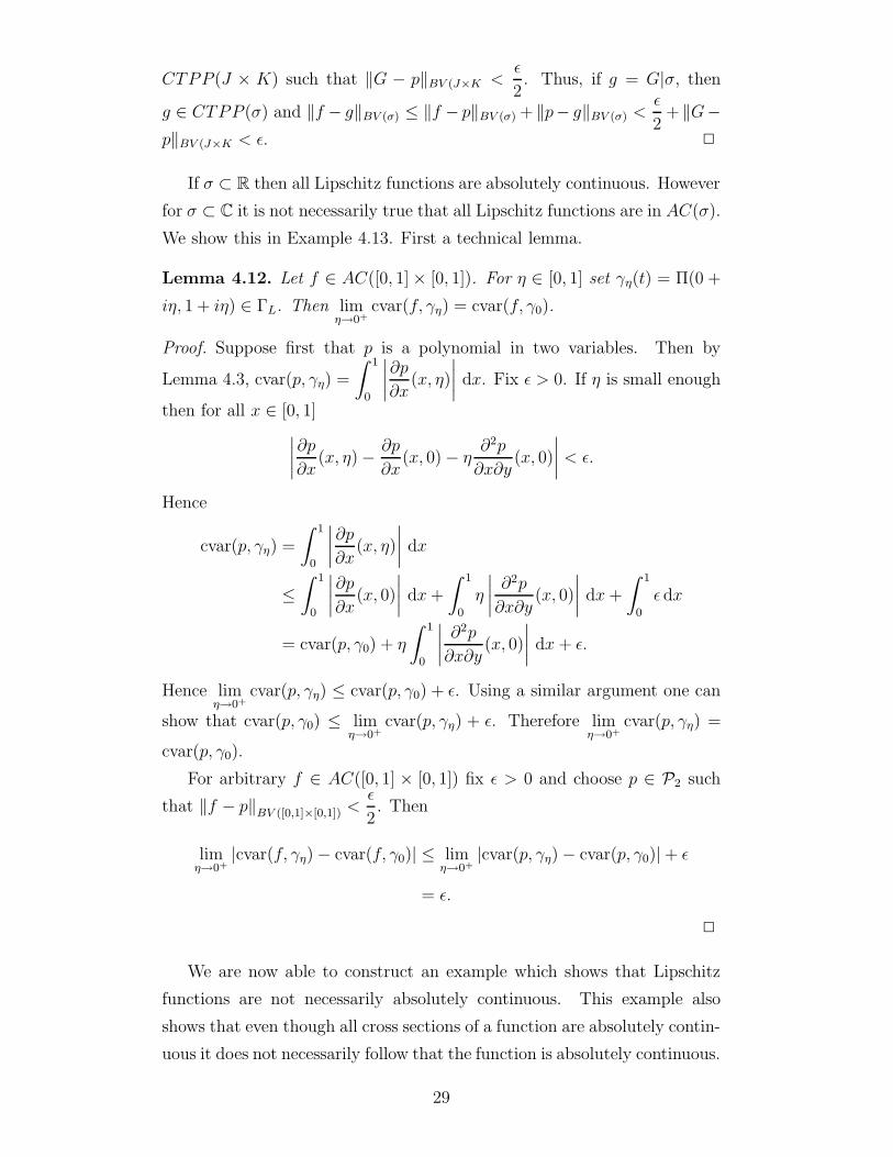
We show this in Example 4.13. First a technical lemma.
Lemma 4.12. Let f ∈ AC([0, 1] × [0, 1]). For η ∈ [0, 1] set γη(t) = Π(0 +
iη, 1 + iη) ∈ ΓL. Then limη→0+
cvar(f, γη) = cvar(f, γ0).
Proof. Suppose first that p is a polynomial in two variables. Then by
Lemma 4.3, cvar(p, γη) =
∫ 1
0
∣
∣
∣
∣
∂p
∂x(x, η)
∣
∣
∣
∣
dx. Fix ε > 0. If η is small enough
then for all x ∈ [0, 1]∣
∣
∣
∣
∂p
∂x(x, η) − ∂p
∂x(x, 0) − η
∂2p
∂x∂y(x, 0)
∣
∣
∣
∣
< ε.
Hence
cvar(p, γη) =
∫ 1
0
∣
∣
∣
∣
∂p
∂x(x, η)
∣
∣
∣
∣
dx
≤∫ 1
0
∣
∣
∣
∣
∂p
∂x(x, 0)
∣
∣
∣
∣
dx +
∫ 1
0
η
∣
∣
∣
∣
∂2p
∂x∂y(x, 0)
∣
∣
∣
∣
dx +
∫ 1
0
ε dx
= cvar(p, γ0) + η
∫ 1
0
∣
∣
∣
∣
∂2p
∂x∂y(x, 0)
∣
∣
∣
∣
dx + ε.
Hence limη→0+
cvar(p, γη) ≤ cvar(p, γ0) + ε. Using a similar argument one can
show that cvar(p, γ0) ≤ limη→0+
cvar(p, γη) + ε. Therefore limη→0+
cvar(p, γη) =
cvar(p, γ0).
For arbitrary f ∈ AC([0, 1] × [0, 1]) fix ε > 0 and choose p ∈ P2 such
that ‖f − p‖BV ([0,1]×[0,1]) <ε
2. Then
limη→0+
|cvar(f, γη) − cvar(f, γ0)| ≤ limη→0+
|cvar(p, γη) − cvar(p, γ0)| + ε
= ε.
2
We are now able to construct an example which shows that Lipschitz
functions are not necessarily absolutely continuous. This example also
shows that even though all cross sections of a function are absolutely contin-
uous it does not necessarily follow that the function is absolutely continuous.
29

Example 4.13. For each n ∈ N let ln = [0, 1] ×{
1
2n
}
. Let hn : [0, 1] →R be the sawtooth function with n teeth, each of height 1 and such that
h(0) = 0. For each ln define f(
x,1
2n
)
=hn(x)
2n+1. Define f([0, 1] × {0}) = 0.
Then f ∈ Lip(∪nln) with L(f) = 1. Now f can be extended to a function
F : [0, 1]×[0, 1] → R such that l(F ) = 1. If γ 1
nare defined as in Lemma 4.12
then cvar(F, γ 1
n) = L(F ) = 1 for all n ∈ N. But cvar(F, γ0) = 0. Hence by
Lemma 4.12, F 6∈ AC([0, 1] × [0, 1]). Also note that for all γ ∈ ΓL where
γ(0), γ(1) ∈ J × K then ι(F ◦ γ) ∈ Lip([0, 1]) ⊂ AC([0, 1]).
5 Operator theory
We shall say that an operator T ∈ B(X) is an AC(σ) operator if it admits
an AC(σ) functional calculus; that is, if there exists a continuous Banach
algebra homomorphism Ψ : AC(σ) → B(X) such that Ψ(1) = I and Ψ(λ) =
T . It is easy to see that if T is a normal operator on a Hilbert space, or more
generally, a scalar-type spectral operator, then T is an AC(σ(T )) operator.
As we noted in the introduction, the theory of AC(σ) operators will be
pursued more fully in [3] and [4]. There are however a few results which are
worth recording here. The first is to confirm that this theory does indeed
generalize the well-bounded theory. The ‘if’ part of the next theorem follows
from Lemmas 3.9 and 4.5. For the converse direction, it is obvious that
every well-bounded operator is an AC(σ) operator. That one can choose
σ = σ(T ) is shown in [2] or [3].
Theorem 5.1. On operator T ∈ B(X) is well-bounded if and only if it is
an AC(σ(T )) operator and σ(T ) ⊂ R.
Part of the motivation for the our new definitions was to ensure that
the class of AC(σ) operators is closed under affine transformations. The
following is an immediate consequence of Theorem 4.1.
Theorem 5.2. If T ∈ B(X) is an AC(σ) operator then for all α, β ∈ C,
αT + βI is an AC(ασ + β) operator.
Berkson and Gillespie [7] defined an operator to be an AC operator
if it admits a functional calculus for the algebra of functions which are
absolutely continuous in the Hardy-Krause sense. We show in [4] that given
30
any rectangle J × K, ACHK(J × K) ⊂ AC(J × K) and that the inclusion
map is continuous. An immediate consequence is the following theorem.
Theorem 5.3. If T ∈ B(X) is an AC(σ) operator then T is an AC operator
(in the sense of Berkson and Gillespie), and hence there exist commuting
well-bounded operators A, B ∈ B(X) such that T = A + iB.
The converse of this theorem is false. The example from [6] of an AC
operator T such that (1 + i)T is not an AC operator gives an example of
an AC operator which is not an AC(σ) operator (for any σ).
One of the most important subclasses of AC operators has been the
family of trigonometrically well-bounded operators. The following result is
a consequence of Proposition 3.11 and the definition of being trigonometri-
cally well-bounded [8].
Theorem 5.4. Every trigonometrically well-bounded operator is an AC(T)
operator.
It is true, but slightly delicate to prove, that the norm on BV (T) is
equivalent to the natural one introduced in [8]. Consequently, on reflex-
ive Banach spaces, AC(T) operators are precisely trigonometrically well-
bounded operators. Details will appear in [3] and [4].
References
[1] L. Ambrosio, ‘A compactness theorem for a new class of functions of
bounded variation’, Boll. Un. Mat. Ital. B (7) 3 (1989), 857–881.
[2] B. Ashton, Functions of bounded variation in two variables and AC(σ)
operators, Ph.D. thesis, University of New South Wales, 2000.
[3] B. Ashton, ‘AC(σ) operators’, (preprint).
[4] B. Ashton and I. Doust, ‘A comparison of algebras of functions of
bounded variation’, (submitted) [Available at
http://www.maths.unsw.edu.au/∼iand/Papers/Compbv/ ].
[5] H. Benzinger, E. Berkson and T. A. Gillespie, ‘Spectral families of pro-
jections, semigroups, and differential operators’, Trans. Amer. Math.
Soc. 275 (1983), 431–475.
31
[6] E. Berkson, I. Doust and T. A. Gillespie, ‘Properties of AC-operators’,
Acta Sci. Math. (Szeged) 6 (1997), 249–271.
[7] E. Berkson and T. A. Gillespie, ‘Absolutely continuous functions of
two variables and well-bounded operators’, J. London Math. Soc. (2)
30 (1984), 305-321.
[8] E. Berkson and T. A. Gillespie, ‘AC functions on the circle and spectral
families’, J. Operator Theory 13 (1985) 33-47.
[9] J. A. Clarkson and C. R. Adams, ‘On definitions of bounded variation
for functions of two variables’, Trans. Amer. Math. Soc. 35 (1933),
824-854.
[10] H. R. Dowson, Spectral theory of linear operators, London Mathemat-
ical Society Monographs 12, Academic Press, London, 1978.
[11] E. W. Hobson, The Theory of Functions of a Real Variable and the The-
ory of Fourier Series, Third Edition, Dover Publications, New York,
1927.
[12] I. P. Natanson, Theory of Functions Of A Real Variable, Frederick
Ungar Publishing Company, New York, 1955.
[13] J. R. Ringrose, ‘On well-bounded operators II’, Proc. London Math.
Soc. (3), 13 (1963), 613-638.
[14] H. L. Royden, Real Analysis, Second Edition, Macmillan Publishing
Company, New York, 1968.
[15] D. R. Smart, ‘Conditionally convergent spectral expansions’, J. Aus-
tral. Math. Soc. (Series A) 1 (1960), 319-333.
[16] E. M. Stein, Singular Integrals And Differentiability Properties Of
Functions, Princeton University Press, Princeton, New Jersey 1970.
[17] J. Wilson, ‘The relationship between polar and AC operators’, Glasg.
Math. J. 41 (1999), 431–439.
32