Final Exam

Revision

Make Money Fast!

StockFraud

PonziScheme

BankRobbery

01234 451-229-0004

981-101-0002

025-612-0001

6

3 8

4

vz

ORD

DFW

SFO

LAX

802

1743

1843

1233

337

DB

A

C

E

Revision 2

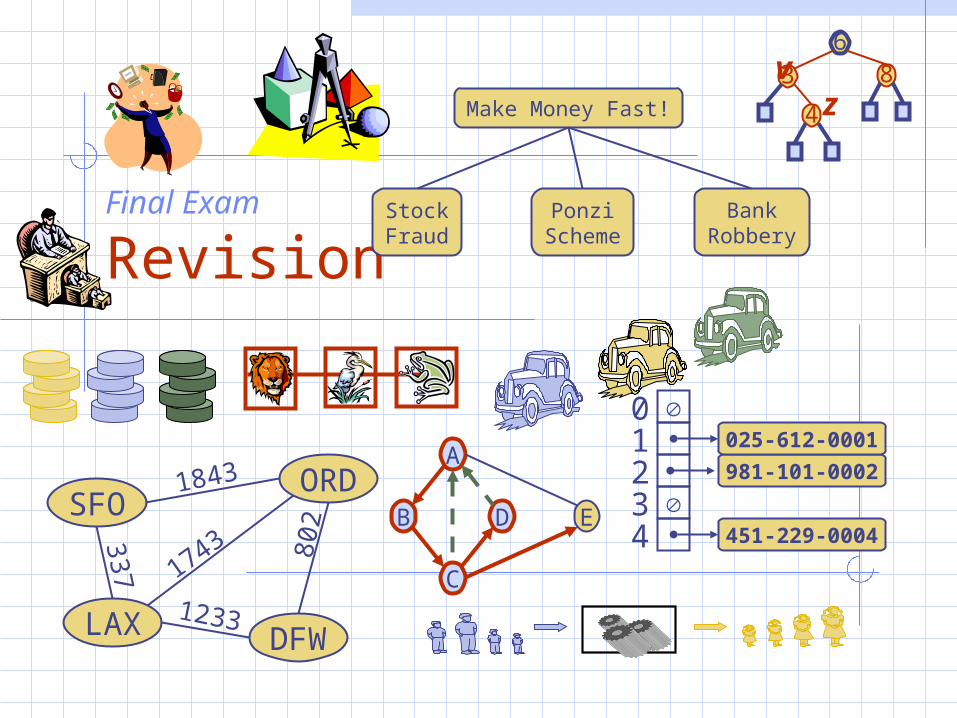
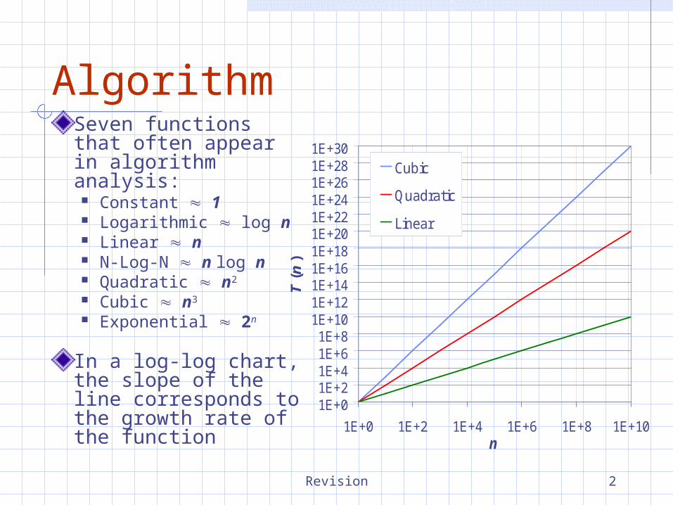
AlgorithmSeven functions that often appear in algorithm analysis:

Constant 1 Logarithmic log n Linear n N-Log-N n log n Quadratic n2

Cubic n3

Exponential 2n

In a log-log chart, the slope of the line corresponds to the growth rate of the function

1E+01E+21E+41E+61E+8

1E+101E+121E+141E+161E+181E+201E+221E+241E+261E+281E+30

1E+0 1E+2 1E+4 1E+6 1E+8 1E+10n

T(n

)

Cubic

Quadratic

Linear

Revision 3

PseudocodeHigh-level description of an algorithmMore structured than English proseLess detailed than a programPreferred notation for describing algorithmsHides program design issues

Algorithm arrayMax(A, n)Input array A of n integersOutput maximum element of A

currentMax A[0]for i 1 to n 1 do

if A[i] currentMax thencurrentMax A[i]

return currentMax

Example: find max element of an array

Revision 4

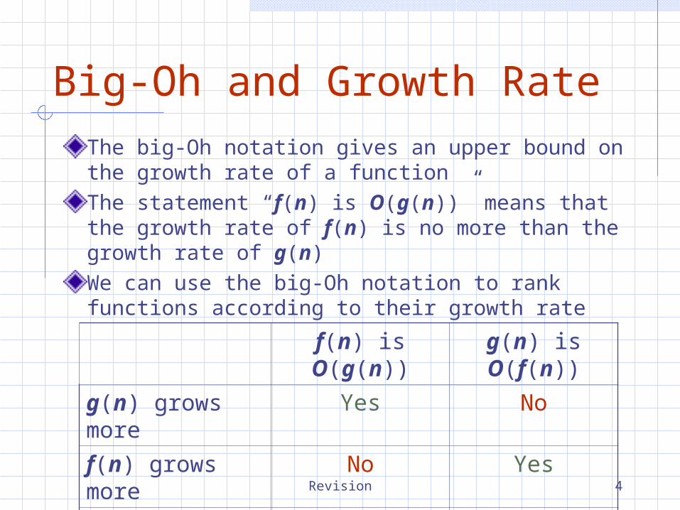
Big-Oh and Growth RateThe big-Oh notation gives an upper bound on the growth rate of a functionThe statement “f(n) is O(g(n))” means that the growth rate of f(n) is no more than the growth rate of g(n)

We can use the big-Oh notation to rank functions according to their growth rate

f(n) is O(g(n)) g(n) is O(f(n))

g(n) grows more

Yes No

f(n) grows more No Yes

Same growth Yes Yes

Revision 5

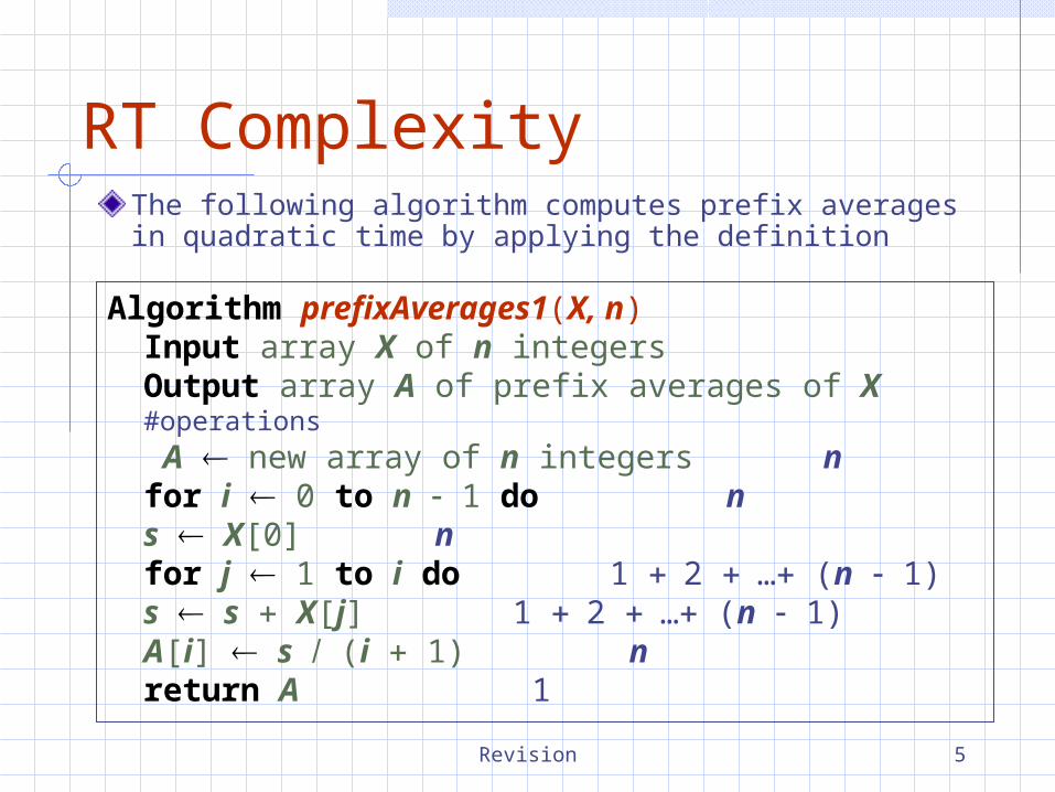
RT ComplexityThe following algorithm computes prefix averages in quadratic time by applying the definition

Algorithm prefixAverages1(X, n)Input array X of n integersOutput array A of prefix averages of X #operations A new array of n integers nfor i 0 to n 1 do n

s X[0] nfor j 1 to i do 1 2 … (n 1)

s s X[j] 1 2 … (n 1)A[i] s (i 1) n

return A 1

Revision 6

Recursion and its Complexity

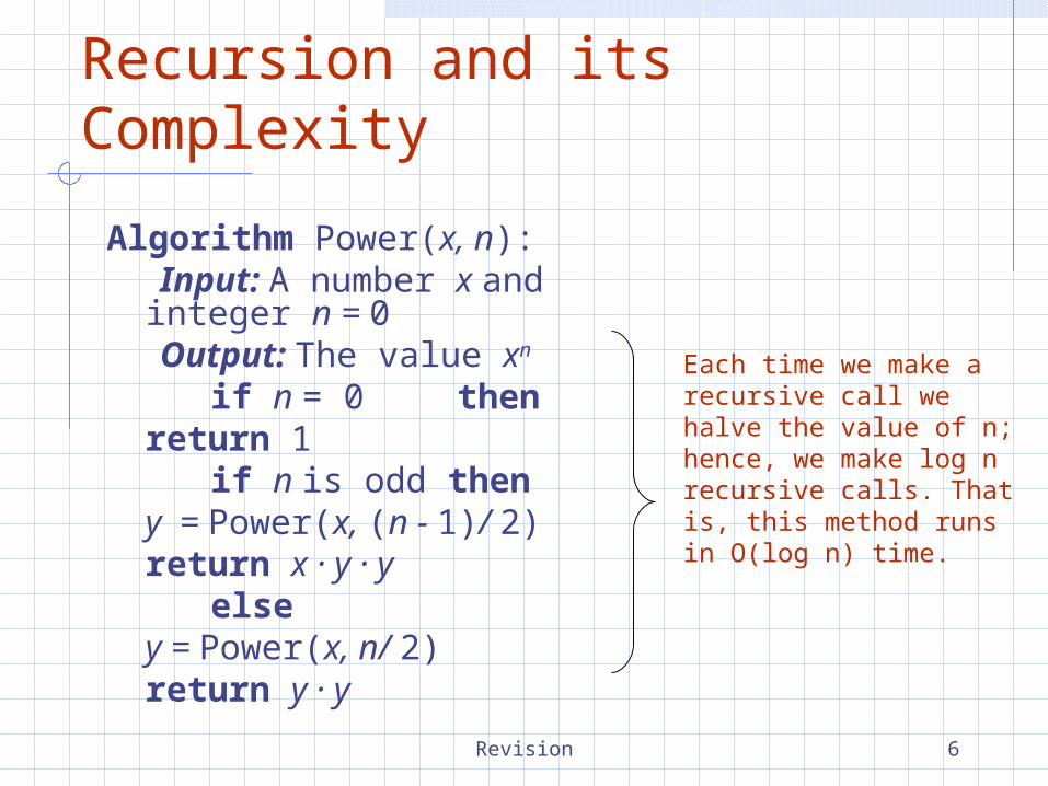
Algorithm Power(x, n): Input: A number x and

integer n = 0 Output: The value xn

if n = 0 thenreturn 1

if n is odd theny = Power(x, (n - 1)/

2)return x · y · y

elsey = Power(x, n/ 2)return y · y

Each time we make a recursive call we halve the value of n; hence, we make log n recursive calls. That is, this method runs in O(log n) time.

Revision 7

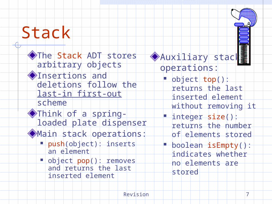
StackThe Stack ADT stores arbitrary objectsInsertions and deletions follow the last-in first-out schemeThink of a spring-loaded plate dispenserMain stack operations:

push(object): inserts an element

object pop(): removes and returns the last inserted element

Auxiliary stack operations:

object top(): returns the last inserted element without removing it

integer size(): returns the number of elements stored

boolean isEmpty(): indicates whether no elements are stored

Revision 8

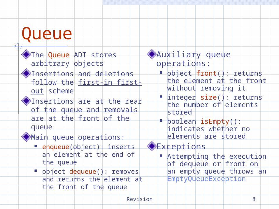
QueueThe Queue ADT stores arbitrary objectsInsertions and deletions follow the first-in first-out schemeInsertions are at the rear of the queue and removals are at the front of the queueMain queue operations:

enqueue(object): inserts an element at the end of the queue

object dequeue(): removes and returns the element at the front of the queue

Auxiliary queue operations:

object front(): returns the element at the front without removing it

integer size(): returns the number of elements stored

boolean isEmpty(): indicates whether no elements are stored

Exceptions Attempting the execution

of dequeue or front on an empty queue throws an EmptyQueueException

Revision 9

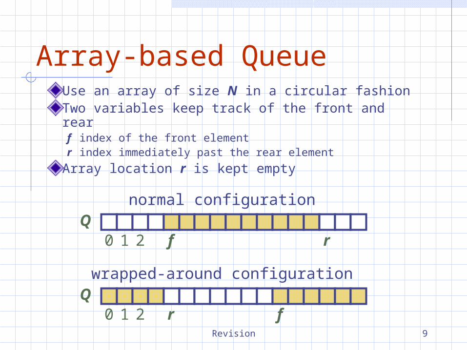
Array-based QueueUse an array of size N in a circular fashionTwo variables keep track of the front and rearf index of the front elementr index immediately past the rear element

Array location r is kept empty

Q0 1 2 rf

normal configuration

Q0 1 2 fr

wrapped-around configuration

Revision 10

Doubly Linked ListA doubly linked list provides a natural implementation of the List ADTNodes implement Position and store:

element link to the previous node link to the next node

Special trailer and header nodes

prev next

elem

trailerheader nodes/positions

elements

node

Revision 11

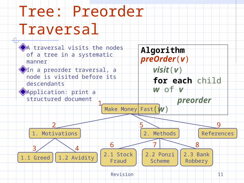
Tree: Preorder TraversalA traversal visits the nodes of a tree in a systematic mannerIn a preorder traversal, a node is visited before its descendants Application: print a structured document

Make Money Fast!

1. Motivations References2. Methods

2.1 StockFraud

2.2 PonziScheme

1.1 Greed 1.2 Avidity2.3 BankRobbery

1

2

3

5

4 6 7 8

9

Algorithm preOrder(v)visit(v)for each child w of v

preorder (w)

Revision 12

Tree: Postorder TraversalIn a postorder traversal, a node is visited after its descendantsApplication: compute space used by files in a directory and its subdirectories

Algorithm postOrder(v)for each child w of v

postOrder (w)visit(v)

cs16/

homeworks/todo.txt

1Kprograms/

DDR.java10K

Stocks.java25K

h1c.doc3K

h1nc.doc2K

Robot.java20K

9

3

1

7

2 4 5 6

8

Revision 13

Tree: Inorder TraversalIn an inorder traversal a node is visited after its left subtree and before its right subtree

Algorithm inOrder(v)if hasLeft (v)

inOrder (left (v))visit(v)if hasRight (v)

inOrder (right (v))

3

1

2

5

6

7 9

8

4

Revision 14

Properties of Proper Binary Trees

Notationn number of nodese number of

external nodesi number of

internal nodesh height

Properties: e i 1 n 2e 1 h i h (n 1)2 e 2h

h log2 e

h log2 (n 1) 1

Revision 15

Priority Queue

A priority queue stores a collection of entriesEach entry is a pair(key, value)Main methods of the Priority Queue ADT

insert(k, x)inserts an entry with key k and value x

removeMin()removes and returns the entry with smallest key

Additional methods min()

returns, but does not remove, an entry with smallest key

size(), isEmpty()

Applications: Standby flyers Auctions Stock market

Revision 16

Sequence-based Priority Queue

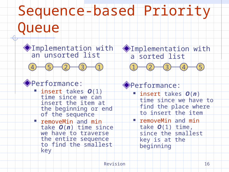
Implementation with an unsorted list

Performance: insert takes O(1) time

since we can insert the item at the beginning or end of the sequence

removeMin and min take O(n) time since we have to traverse the entire sequence to find the smallest key

Implementation with a sorted list

Performance: insert takes O(n) time

since we have to find the place where to insert the item

removeMin and min take O(1) time, since the smallest key is at the beginning

4 5 2 3 1 1 2 3 4 5

Revision 17

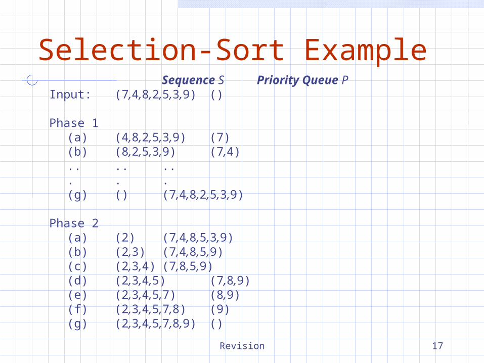
Selection-Sort Example Sequence S Priority Queue PInput: (7,4,8,2,5,3,9) ()

Phase 1(a) (4,8,2,5,3,9) (7)(b) (8,2,5,3,9) (7,4).. .. ... . .(g) () (7,4,8,2,5,3,9)

Phase 2(a) (2) (7,4,8,5,3,9)(b) (2,3) (7,4,8,5,9)(c) (2,3,4) (7,8,5,9)(d) (2,3,4,5) (7,8,9)(e) (2,3,4,5,7) (8,9)(f) (2,3,4,5,7,8) (9)(g) (2,3,4,5,7,8,9) ()

Revision 18

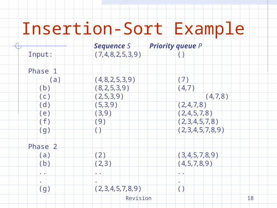
Insertion-Sort ExampleSequence S Priority queue P

Input: (7,4,8,2,5,3,9) ()

Phase 1 (a) (4,8,2,5,3,9) (7)

(b) (8,2,5,3,9) (4,7)(c) (2,5,3,9) (4,7,8)(d) (5,3,9) (2,4,7,8)(e) (3,9) (2,4,5,7,8)(f) (9) (2,3,4,5,7,8)(g) () (2,3,4,5,7,8,9)

Phase 2(a) (2) (3,4,5,7,8,9)(b) (2,3) (4,5,7,8,9).. .. ... . .(g) (2,3,4,5,7,8,9) ()

Revision 19

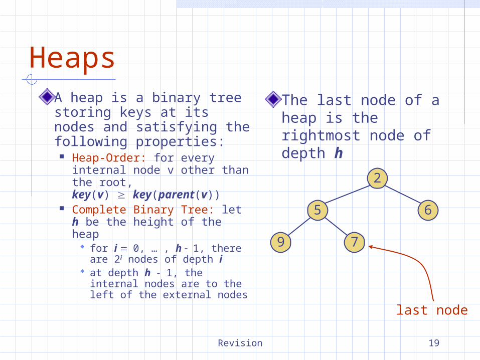
HeapsA heap is a binary tree storing keys at its nodes and satisfying the following properties:

Heap-Order: for every internal node v other than the root,key(v) key(parent(v))

Complete Binary Tree: let h be the height of the heap

for i 0, … , h 1, there are 2i nodes of depth i

at depth h 1, the internal nodes are to the left of the external nodes

2

65

79

The last node of a heap is the rightmost node of depth h

last node

Revision 20

Height of a HeapTheorem: A heap storing n keys has height O(log n)

Proof: (we apply the complete binary tree property) Let h be the height of a heap storing n keys Since there are 2i keys at depth i 0, … , h 1 and at least

one key at depth h, we have n 1 2 4 … 2h1 1

Thus, n 2h , i.e., h log n

1

2

2h1

1

keys

0

1

h1

h

depth

Revision 21

Heap-Sort

Consider a priority queue with n items implemented by means of a heap

the space used is O(n) methods insert and

removeMin take O(log n) time

methods size, isEmpty, and min take time O(1) time

Using a heap-based priority queue, we can sort a sequence of n elements in O(n log n) timeThe resulting algorithm is called heap-sortHeap-sort is much faster than quadratic sorting algorithms, such as insertion-sort and selection-sort

Revision 22

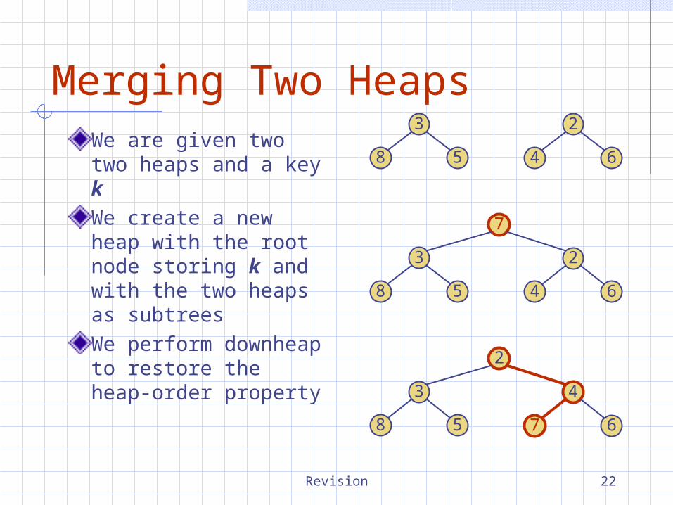
Merging Two HeapsWe are given two two heaps and a key kWe create a new heap with the root node storing k and with the two heaps as subtreesWe perform downheap to restore the heap-order property

7

3

58

2

64

3

58

2

64

2

3

58

4

67

Revision 23

Hash Functions and Hash Tables

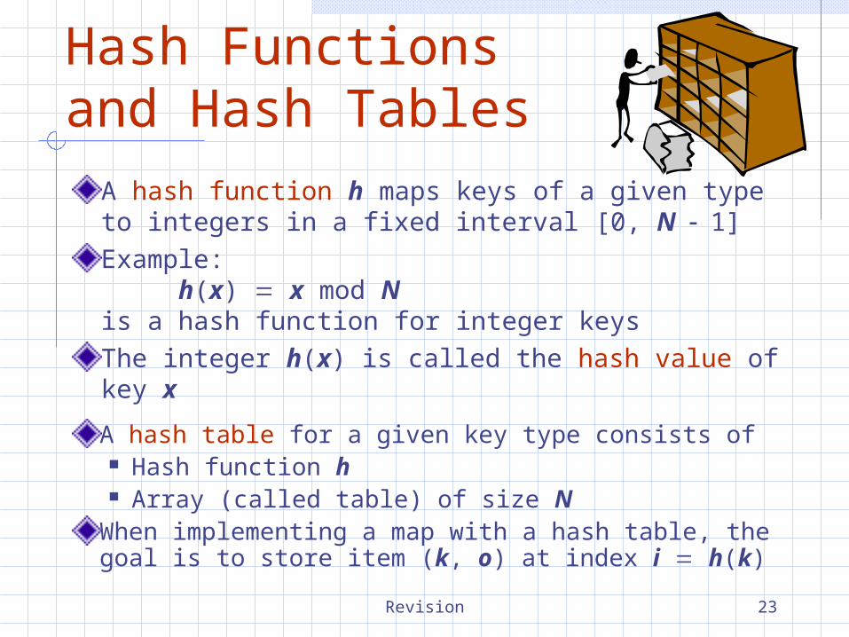
A hash function h maps keys of a given type to integers in a fixed interval [0, N1]

Example:h(x) x mod N

is a hash function for integer keysThe integer h(x) is called the hash value of key x

A hash table for a given key type consists of Hash function h Array (called table) of size N

When implementing a map with a hash table, the goal is to store item (k, o) at index i h(k)

Revision 24

Collision Handling

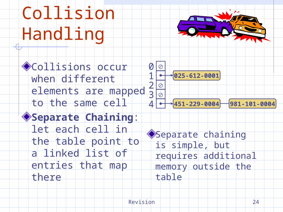
Collisions occur when different elements are mapped to the same cellSeparate Chaining: let each cell in the table point to a linked list of entries that map there

Separate chaining is simple, but requires additional memory outside the table

01234 451-229-0004 981-101-0004

025-612-0001

Revision 25

Linear ProbingOpen addressing: the colliding item is placed in a different cell of the tableLinear probing handles collisions by placing the colliding item in the next (circularly) available table cellEach table cell inspected is referred to as a “probe”Colliding items lump together, causing future collisions to cause a longer sequence of probes

Example: h(x) x mod 13 Insert keys 18, 41,

22, 44, 59, 32, 31, 73, in this order

0 1 2 3 4 5 6 7 8 9 10 11 12

41 18445932223173 0 1 2 3 4 5 6 7 8 9 10 11 12

Revision 26

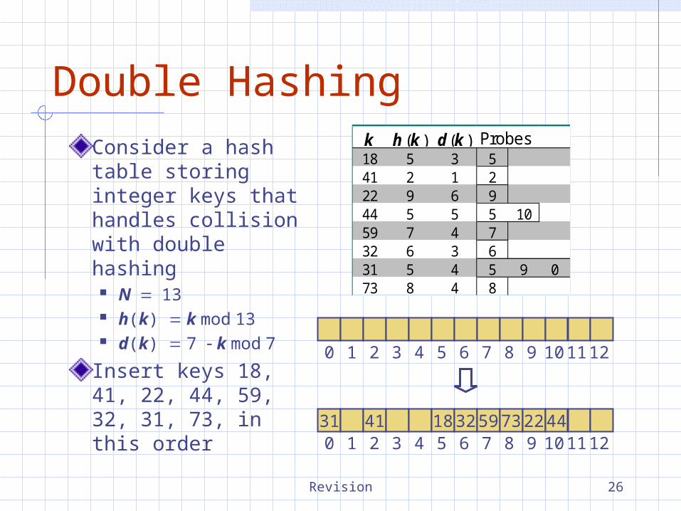
Consider a hash table storing integer keys that handles collision with double hashing

N13 h(k) k mod 13 d(k) 7 k mod 7

Insert keys 18, 41, 22, 44, 59, 32, 31, 73, in this order

Double Hashing

0 1 2 3 4 5 6 7 8 9 10 11 12

31 41 183259732244 0 1 2 3 4 5 6 7 8 9 10 11 12

k h (k ) d (k ) Probes18 5 3 541 2 1 222 9 6 944 5 5 5 1059 7 4 732 6 3 631 5 4 5 9 073 8 4 8

Revision 27

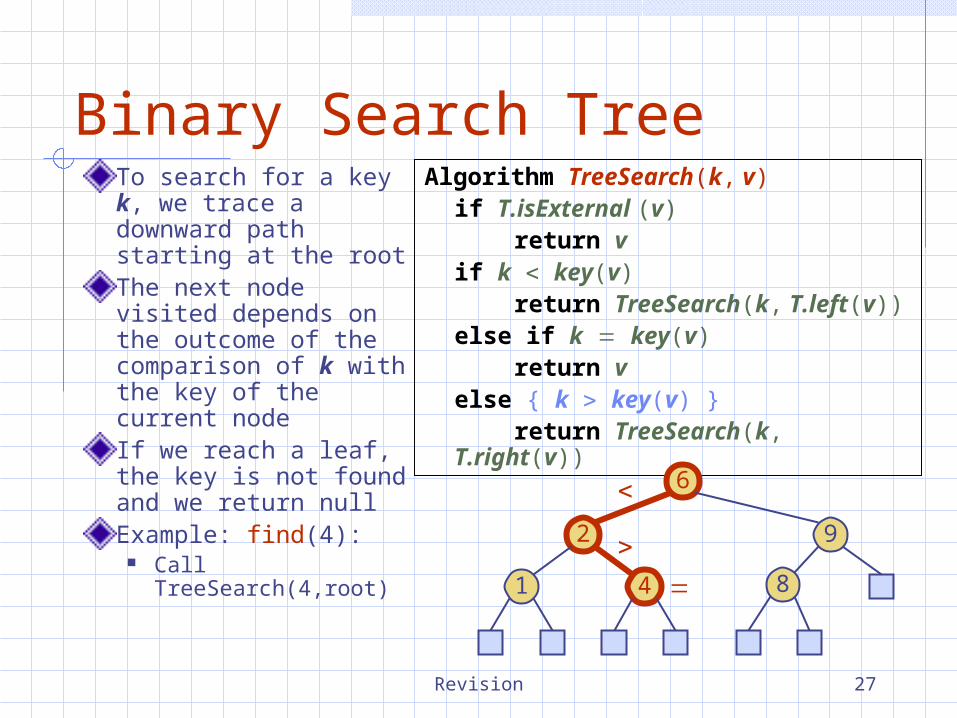
Binary Search TreeTo search for a key k, we trace a downward path starting at the rootThe next node visited depends on the outcome of the comparison of k with the key of the current nodeIf we reach a leaf, the key is not found and we return nullExample: find(4):

Call TreeSearch(4,root)

Algorithm TreeSearch(k, v)if T.isExternal (v)

return vif k key(v)

return TreeSearch(k, T.left(v))else if k key(v)

return velse { k key(v) }

return TreeSearch(k, T.right(v))

6

92

41 8

Revision 28

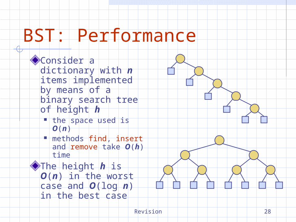
BST: PerformanceConsider a dictionary with n items implemented by means of a binary search tree of height h

the space used is O(n) methods find, insert

and remove take O(h) time

The height h is O(n) in the worst case and O(log n) in the best case

Revision 29

AVL Tree

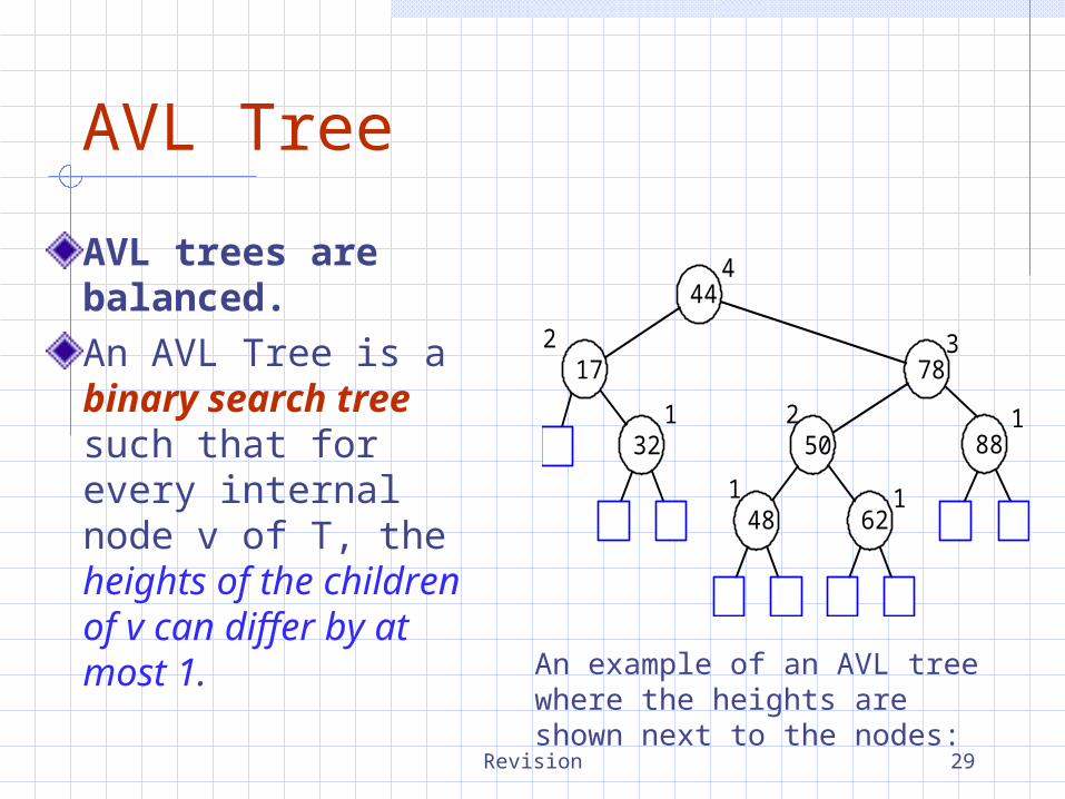
AVL trees are balanced.An AVL Tree is a binary search tree such that for every internal node v of T, the heights of the children of v can differ by at most 1.

88

44

17 78

32 50

48 62

2

4

1

1

2

3

1

1

An example of an AVL tree where the heights are shown next to the nodes:

Revision 30

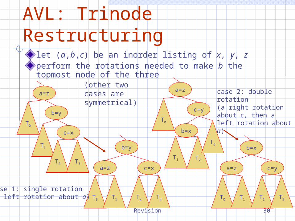
AVL: Trinode Restructuringlet (a,b,c) be an inorder listing of x, y, zperform the rotations needed to make b the topmost node of the three

b=y

a=z

c=x

T0

T1

T2 T3

b=y

a=z c=x

T0 T1 T2 T3

c=y

b=x

a=z

T0

T1 T2

T3b=x

c=ya=z

T0 T1 T2 T3

case 1: single rotation(a left rotation about a)

case 2: double rotation(a right rotation about c, then a left rotation about a)

(other two cases are symmetrical)

Revision 31

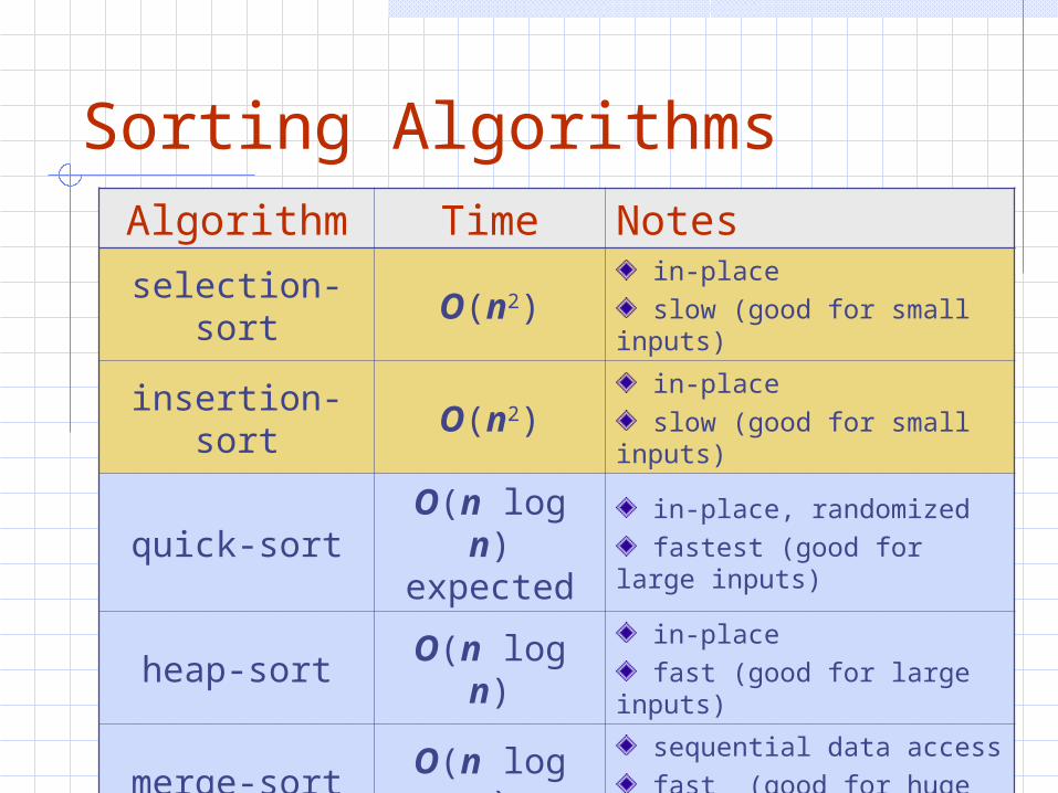
Sorting AlgorithmsAlgorithm Time Notes

selection-sort O(n2) in-place slow (good for small

inputs)

insertion-sort O(n2) in-place slow (good for small

inputs)

quick-sortO(n log n)expected

in-place, randomized fastest (good for large

inputs)

heap-sort O(n log n) in-place fast (good for large inputs)

merge-sort O(n log n) sequential data access fast (good for huge

inputs)

Revision 32

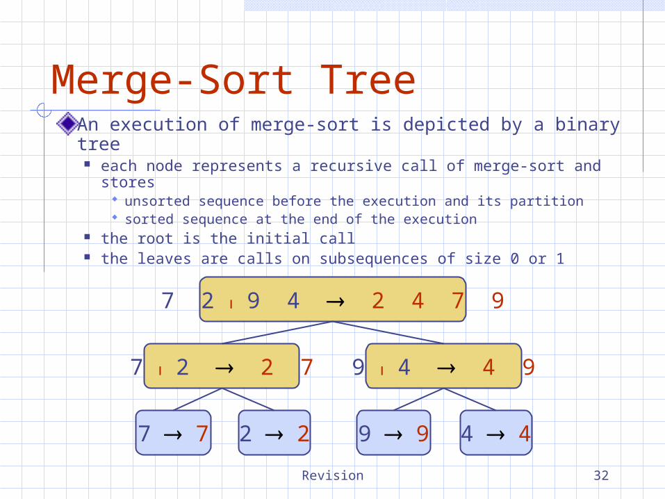
Merge-Sort TreeAn execution of merge-sort is depicted by a binary tree

each node represents a recursive call of merge-sort and stores unsorted sequence before the execution and its partition sorted sequence at the end of the execution

the root is the initial call the leaves are calls on subsequences of size 0 or 1

7 2 9 4 2 4 7 9

7 2 2 7 9 4 4 9

7 7 2 2 9 9 4 4

Revision 33

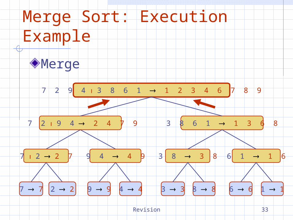
Merge Sort: Execution Example

Merge

7 2 9 4 2 4 7 9 3 8 6 1 1 3 6 8

7 2 2 7 9 4 4 9 3 8 3 8 6 1 1 6

7 7 2 2 9 9 4 4 3 3 8 8 6 6 1 1

7 2 9 4 3 8 6 1 1 2 3 4 6 7 8 9

Revision 34

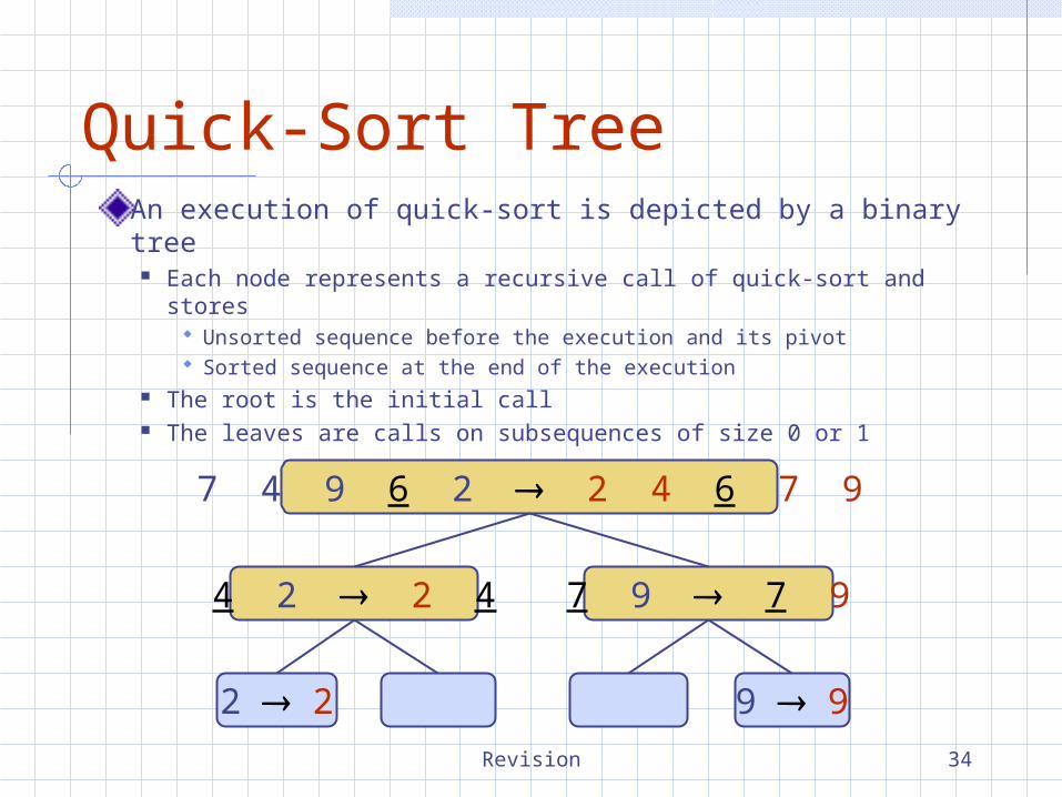
Quick-Sort TreeAn execution of quick-sort is depicted by a binary tree

Each node represents a recursive call of quick-sort and stores Unsorted sequence before the execution and its pivot Sorted sequence at the end of the execution

The root is the initial call The leaves are calls on subsequences of size 0 or 1

7 4 9 6 2 2 4 6 7 9

4 2 2 4 7 9 7 9

2 2 9 9

Revision 35

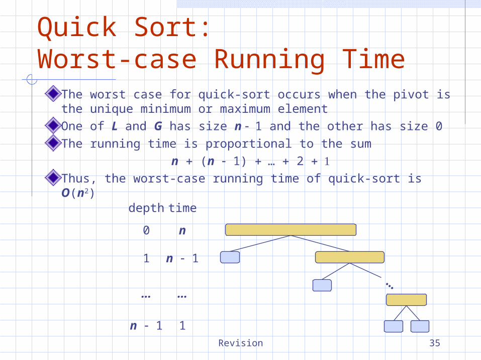
Quick Sort: Worst-case Running Time

The worst case for quick-sort occurs when the pivot is the unique minimum or maximum elementOne of L and G has size n 1 and the other has size 0The running time is proportional to the sum

n (n 1) … 2 Thus, the worst-case running time of quick-sort is O(n2)

depth time

0 n

1 n 1

… …

n 1 1

…

Revision 36

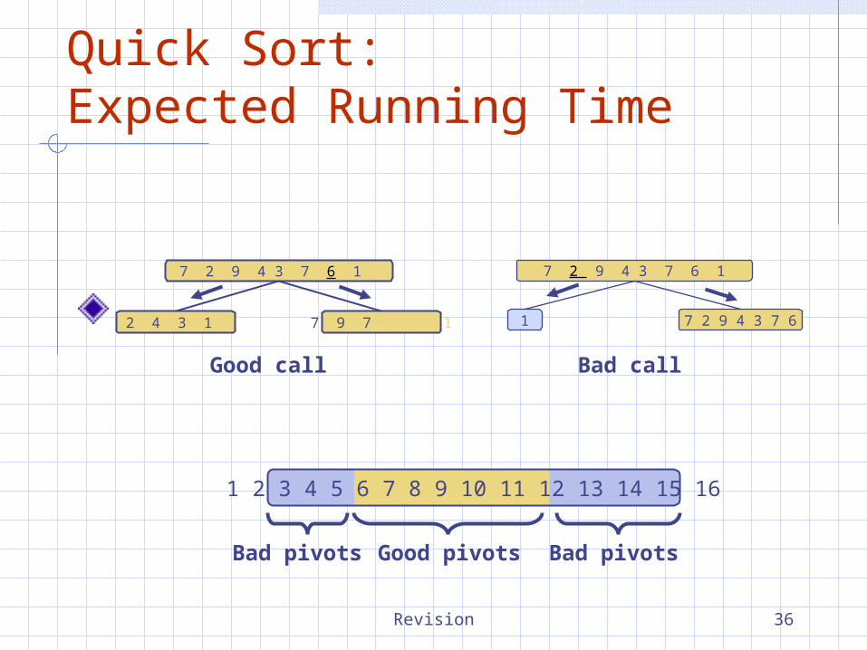
Quick Sort:Expected Running Time

7 9 7 1 1

7 2 9 4 3 7 6 1 9

2 4 3 1 7 2 9 4 3 7 61

7 2 9 4 3 7 6 1

Good call Bad call

1 2 3 4 5 6 7 8 9 10 11 12 13 14 15 16

Good pivotsBad pivots Bad pivots

Revision 37

In-Place Quick-SortQuick-sort can be implemented to run in-placeIn the partition step, we use replace operations to rearrange the elements of the input sequence such that

the elements less than the pivot have rank less than h

the elements equal to the pivot have rank between h and k

the elements greater than the pivot have rank greater than k

The recursive calls consider elements with rank less than h elements with rank greater

than k

Algorithm inPlaceQuickSort(S, l, r)Input sequence S, ranks l and rOutput sequence S with the

elements of rank between l and rrearranged in increasing order

if l r return

i a random integer between l and r x S.elemAtRank(i) (h, k) inPlacePartition(x)inPlaceQuickSort(S, l, h 1)inPlaceQuickSort(S, k 1, r)

Revision 38

In-Place PartitioningPerform the partition using two indices to split S into L and E U G (a similar method can split E U G into E and G).

Repeat until j and k cross: Scan j to the right until finding an element > x. Scan k to the left until finding an element < x. Swap elements at indices j and k

3 2 5 1 0 7 3 5 9 2 7 9 8 9 7 6 9

j k

(pivot = 6)

3 2 5 1 0 7 3 5 9 2 7 9 8 9 7 6 9

j k

Revision 39

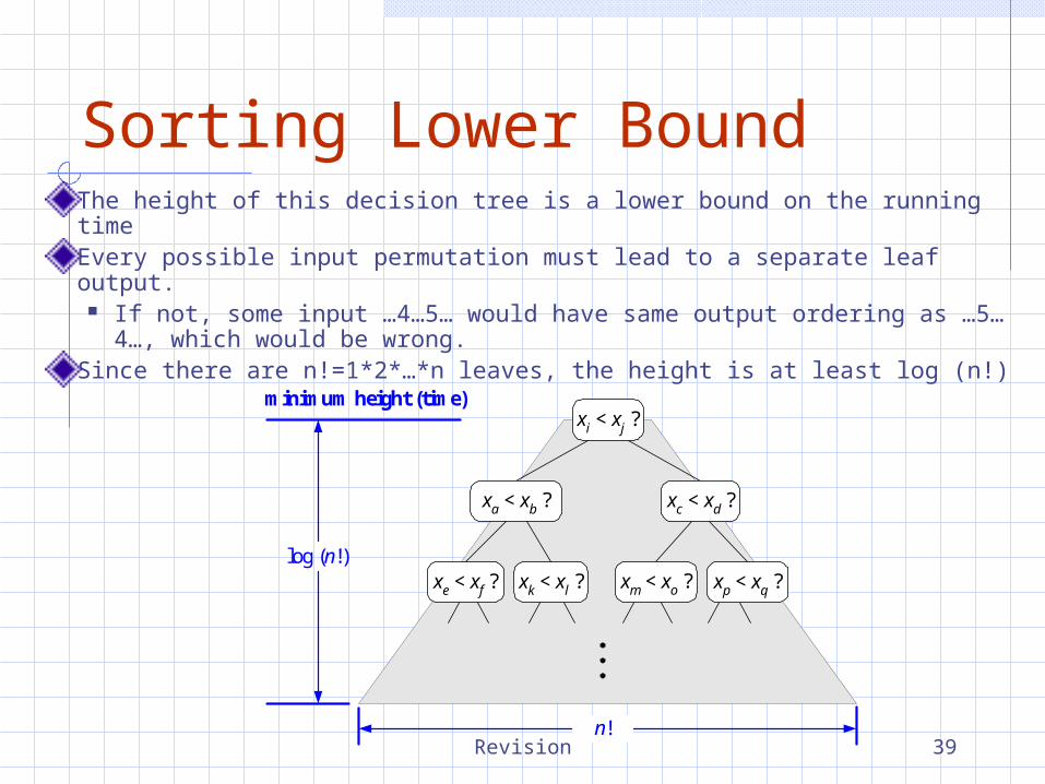
Sorting Lower BoundThe height of this decision tree is a lower bound on the running timeEvery possible input permutation must lead to a separate leaf output.

If not, some input …4…5… would have same output ordering as …5…4…, which would be wrong.

Since there are n!=1*2*…*n leaves, the height is at least log (n!)

minimum height (time)

log (n!)

xi < xj ?

xa < xb ?

xm < xo ? xp < xq ?xe < xf ? xk < xl ?

xc < xd ?

n!

Revision 40

The Lower BoundAny comparison-based sorting algorithms takes at least log (n!) timeTherefore, any such algorithm takes time at least

That is, any comparison-based sorting algorithm must run in Ω(n log n) time.

).2/(log)2/(2

log)!(log2

nnn

n

n

Revision 41

Bucket SortKey range [0, 9]

7, d 1, c 3, a 7, g 3, b 7, e

1, c 3, a 3, b 7, d 7, g 7, e

Phase 1

Phase 2

0 1 2 3 4 5 6 7 8 9

B

1, c 7, d 7, g3, b3, a 7, e

Revision 42

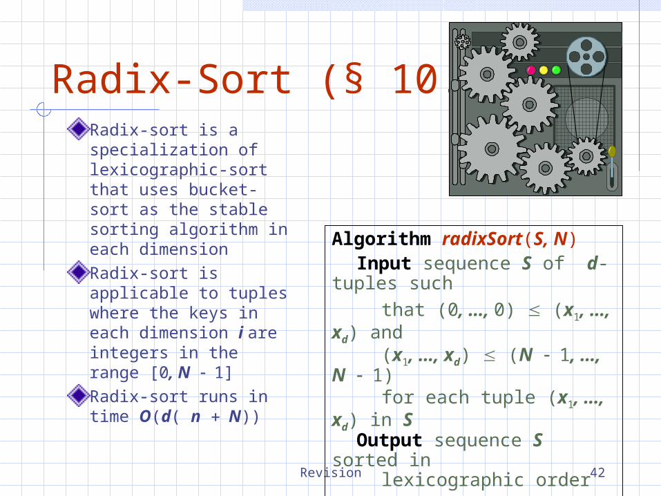
Radix-Sort (§ 10.4.2)Radix-sort is a specialization of lexicographic-sort that uses bucket-sort as the stable sorting algorithm in each dimensionRadix-sort is applicable to tuples where the keys in each dimension i are integers in the range [0, N 1]

Radix-sort runs in time O(d( n N))

Algorithm radixSort(S, N)Input sequence S of d-tuples such

that (0, …, 0) (x1, …, xd) and(x1, …, xd) (N 1, …, N

1)for each tuple (x1, …, xd) in S

Output sequence S sorted inlexicographic order

for i d downto 1bucketSort(S, N)

Revision 43

Radix-Sort for Binary Numbers

Consider a sequence of n b-bit integers

x xb … x1x0

We represent each element as a b-tuple of integers in the range [0, 1] and apply radix-sort with N 2This application of the radix-sort algorithm runs in O(bn) time For example, we can sort a sequence of 32-bit integers in linear time

Algorithm binaryRadixSort(S)Input sequence S of b-bit

integers Output sequence S sortedreplace each element x

of S with the item (0, x)for i 0 to b1

replace the key k of each item (k, x) of Swith bit xi of x

bucketSort(S, 2)

Revision 44

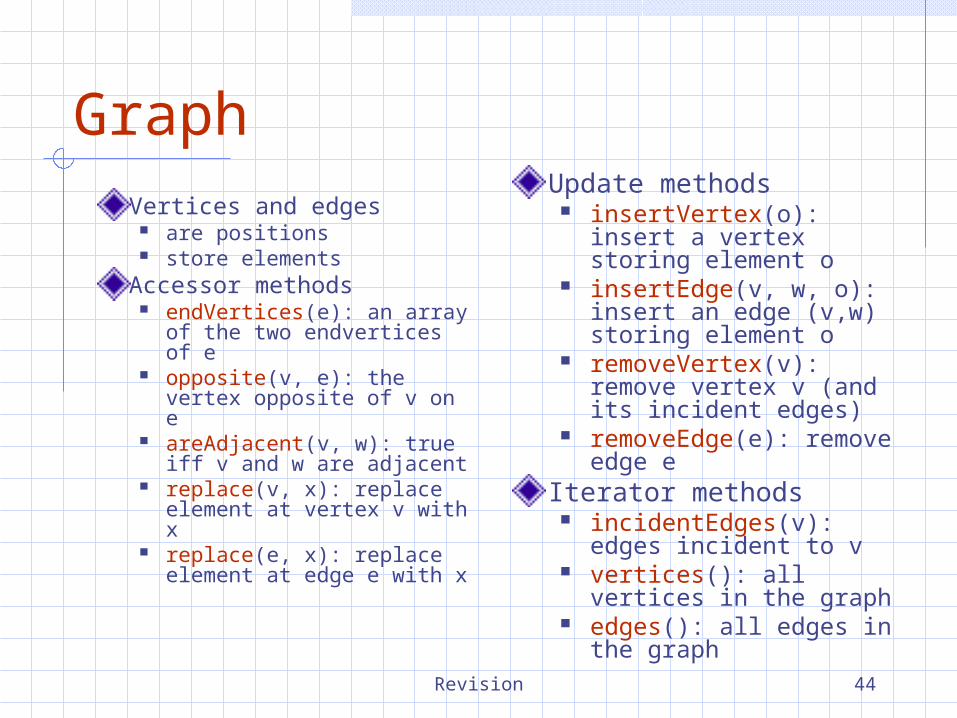
GraphVertices and edges

are positions store elements

Accessor methods endVertices(e): an array

of the two endvertices of e

opposite(v, e): the vertex opposite of v on e

areAdjacent(v, w): true iff v and w are adjacent

replace(v, x): replace element at vertex v with x

replace(e, x): replace element at edge e with x

Update methods insertVertex(o): insert a

vertex storing element o insertEdge(v, w, o):

insert an edge (v,w) storing element o

removeVertex(v): remove vertex v (and its incident edges)

removeEdge(e): remove edge e

Iterator methods incidentEdges(v): edges

incident to v vertices(): all vertices in

the graph edges(): all edges in the

graph

Revision 45

Adjacency List Structure

Incidence sequence for each vertex

sequence of references to edge objects of incident edges

Edge objects references to

associated positions in incidence sequences of end vertices

Revision 46

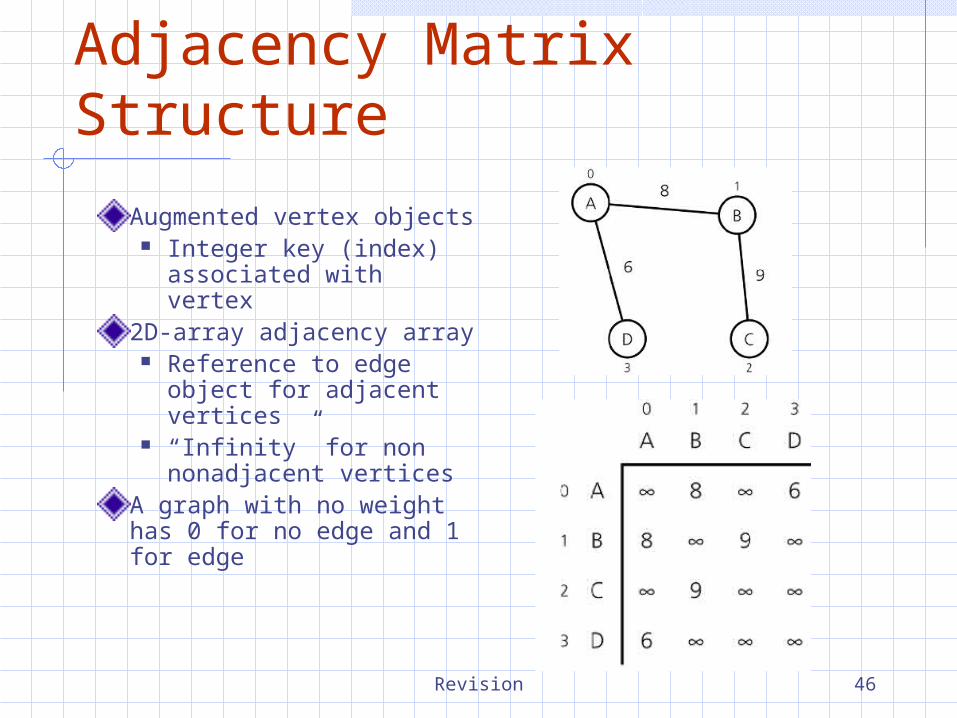
Adjacency Matrix Structure

Augmented vertex objects

Integer key (index) associated with vertex

2D-array adjacency array Reference to edge

object for adjacent vertices

“Infinity” for non nonadjacent vertices

A graph with no weight has 0 for no edge and 1 for edge

Revision 47

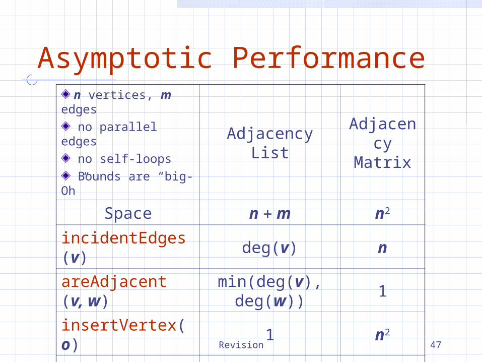
Asymptotic Performance n vertices, m edges no parallel edges no self-loops Bounds are “big-

Oh”

AdjacencyList

Adjacency Matrix

Space n m n2

incidentEdges(v) deg(v) n

areAdjacent (v, w)

min(deg(v), deg(w)) 1

insertVertex(o) 1 n2

insertEdge(v, w, o)

1 1

removeVertex(v)

deg(v) n2

removeEdge(e) 1 1

Revision 48

Depth-First SearchDepth-first search (DFS) is a general technique for traversing a graphA DFS traversal of a graph G

Visits all the vertices and edges of G

Determines whether G is connected

Computes the connected components of G

Computes a spanning forest of G

DFS on a graph with n vertices and m edges takes O(nm ) timeDFS can be further extended to solve other graph problems

Find and report a path between two given vertices

Find a cycle in the graph

Revision 49

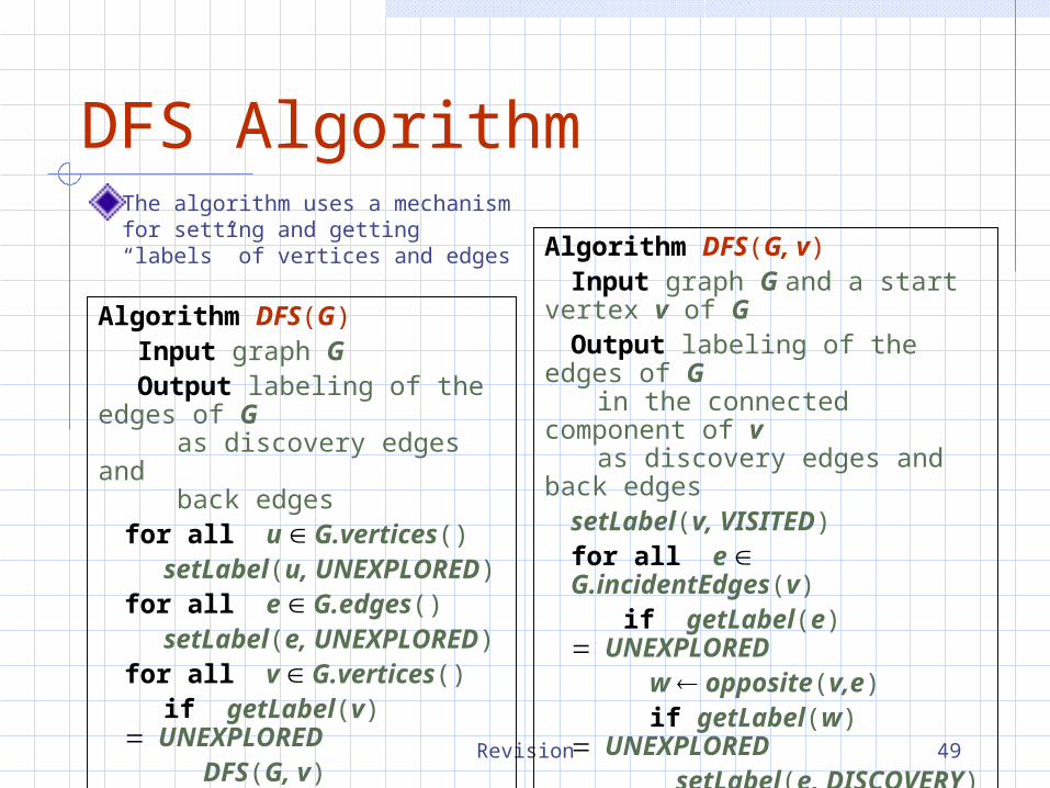
DFS AlgorithmThe algorithm uses a mechanism for setting and getting “labels” of vertices and edges Algorithm DFS(G, v)

Input graph G and a start vertex v of G Output labeling of the edges of G

in the connected component of v as discovery edges and back edges

setLabel(v, VISITED)for all e G.incidentEdges(v)

if getLabel(e) UNEXPLORED

w opposite(v,e)if getLabel(w)

UNEXPLOREDsetLabel(e, DISCOVERY)DFS(G, w)

elsesetLabel(e, BACK)

Algorithm DFS(G)Input graph GOutput labeling of the edges of G

as discovery edges andback edges

for all u G.vertices()setLabel(u, UNEXPLORED)

for all e G.edges()setLabel(e, UNEXPLORED)

for all v G.vertices()if getLabel(v)

UNEXPLOREDDFS(G, v)

Revision 50

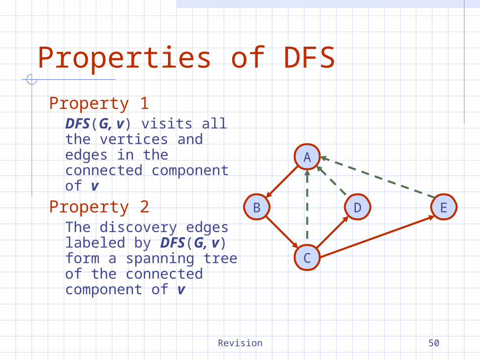
Properties of DFS

Property 1DFS(G, v) visits all the vertices and edges in the connected component of v

Property 2The discovery edges labeled by DFS(G, v) form a spanning tree of the connected component of v

DB

A

C

E

Revision 51

Path FindingWe can specialize the DFS algorithm to find a path between two given vertices u and zWe call DFS(G, u) with u as the start vertexWe use a stack S to keep track of the path between the start vertex and the current vertexAs soon as destination vertex z is encountered, we return the path as the contents of the stack

Algorithm pathDFS(G, v, z)setLabel(v, VISITED)S.push(v)if v z

return S.elements()for all e G.incidentEdges(v)

if getLabel(e) UNEXPLORED

w opposite(v,e)if getLabel(w)

UNEXPLORED setLabel(e, DISCOVERY)S.push(e)pathDFS(G, w, z)S.pop(e)

else setLabel(e, BACK)

S.pop(v)

Revision 52

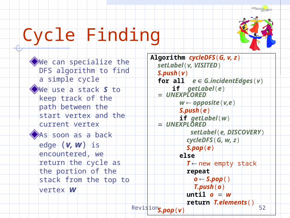
Cycle FindingWe can specialize the DFS algorithm to find a simple cycleWe use a stack S to keep track of the path between the start vertex and the current vertex

As soon as a back edge (v, w) is encountered, we return the cycle as the portion of the stack from the top to vertex w

Algorithm cycleDFS(G, v, z)setLabel(v, VISITED)S.push(v)for all e G.incidentEdges(v)

if getLabel(e) UNEXPLOREDw opposite(v,e)S.push(e)if getLabel(w) UNEXPLORED

setLabel(e, DISCOVERY)cycleDFS(G, w, z)S.pop(e)

elseT new empty stackrepeat

o S.pop()T.push(o)

until o wreturn T.elements()

S.pop(v)

Revision 53

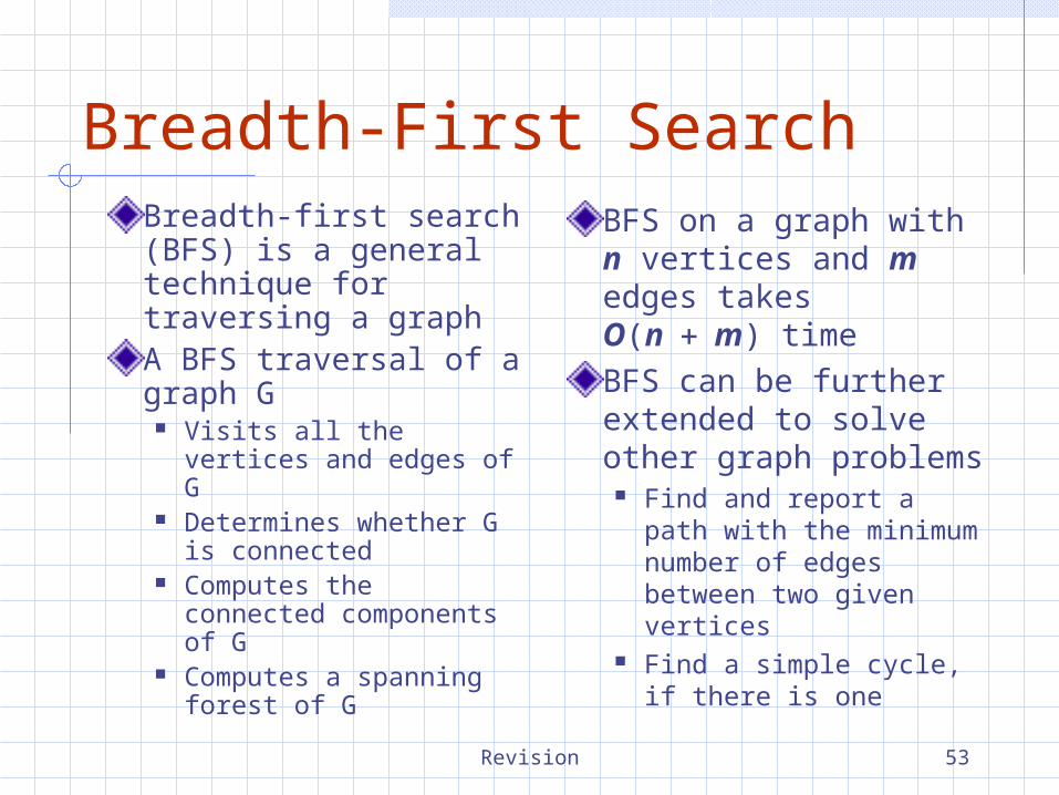
Breadth-First SearchBreadth-first search (BFS) is a general technique for traversing a graphA BFS traversal of a graph G

Visits all the vertices and edges of G

Determines whether G is connected

Computes the connected components of G

Computes a spanning forest of G

BFS on a graph with n vertices and m edges takes O(nm) timeBFS can be further extended to solve other graph problems

Find and report a path with the minimum number of edges between two given vertices

Find a simple cycle, if there is one

Revision 54

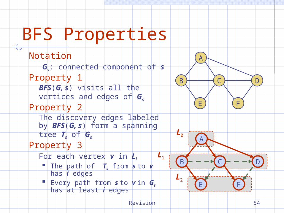
BFS PropertiesNotation

Gs: connected component of s

Property 1BFS(G, s) visits all the vertices and edges of Gs

Property 2The discovery edges labeled by BFS(G, s) form a spanning tree Ts of Gs

Property 3For each vertex v in Li

The path of Ts from s to v has i edges

Every path from s to v in Gs has at least i edges

CB

A

E

D

L0

L1

FL2

CB

A

E

D

F

Revision 55

BFS Applications

Using the template method pattern, we can specialize the BFS traversal of a graph G to solve the following problems in O(n m) time Compute the connected components of G Compute a spanning forest of G Find a simple cycle in G, or report that G is a

forest Given two vertices of G, find a path in G

between them with the minimum number of edges, or report that no such path exists

Revision 56

DFS vs. BFS

CB

A

E

D

L0

L1

FL2

CB

A

E

D

F

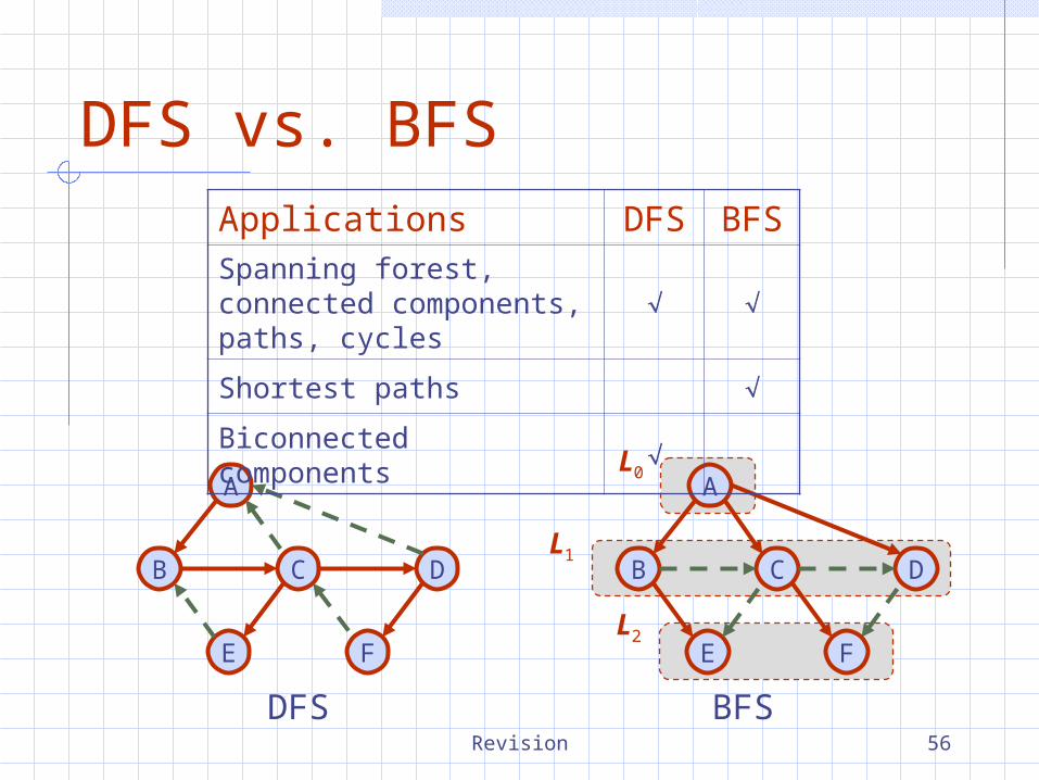
DFS BFS

Applications DFS BFSSpanning forest, connected components, paths, cycles

Shortest paths

Biconnected components