International Baccalaureate

Candidate n~me I L_ ________________________ __

School number

School name

Examination session (May or November) l A ~·-}'-"!

Extended essay cover

I

I

-~_.....l_vear J 2 0) ;;:2.- _

Diploma Programme subject in which this extended essay is registered /l~cs (For an extended essay in the area of languages. state the language and whether it is group 1 or group 2.)

Title of the extended es~ ~6/;~I.A--- 21:~~C: Lf/odou;s ~Jed tl(df!kceL_

Candidate's declaration

This declaration must be signed by the candidate, otherwise a grade may not be rssued

The extended essay I am submitting 1s my own work (apart from guidance allowed by the International Baccalaureate).

I have acknowledged each use of the words, graphics or ideas of another person, whether written, oral or visual.

I am aware that the word limit for all extended essays is 4000 words and that examiners are not required to read beyond th1s limit.

This is the final version of my extended essay

Candidate's signatur Date

International Baccalaureate F>eterson Ho_u_se. ________________________________ _____.

Supervisor's report and declaration

The supervisor must complete this report, sign the declaration and then give the final version of the extended essay, with this cover attached, to the Diploma Programme coordinator.

Name of supervisor (CAPITAL letters)

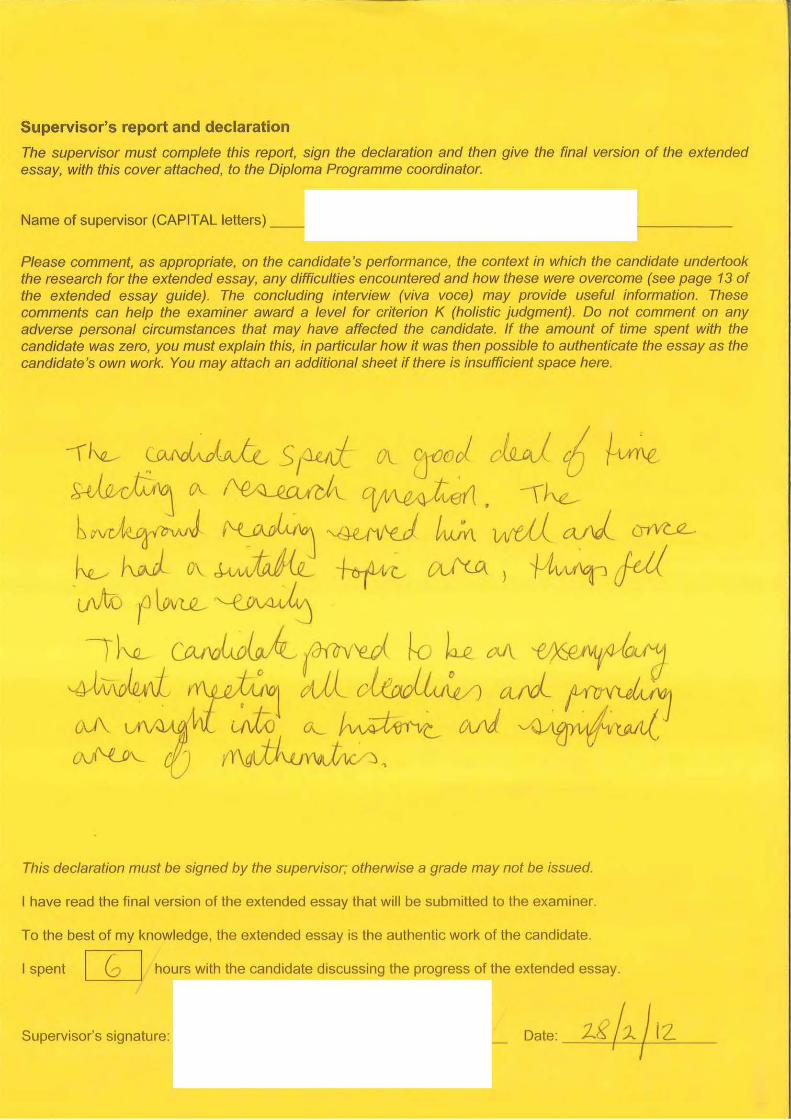
Please comment, as appropriate, on the candidate's performance, the context in which the candidate undertook the research for the extended essay, any difficulties encountered and how these were overcome (see page 13 of the extended essay guide). The concluding interview (viva voce) may provide useful information. These comments can help the examiner award a level for criterion K (holistic judgment). Do not comment on any adverse personal circumstances that may have affected the candidate. If the amount of time spent with the candidate was zero, you must explain this, in particular how it was then possible to authenticate the essay as the candidate's own work. You may attach an additional sheet if there is insufficient space here.

··f/~ ~w-J._~(e__ c;1:u_J L\ C)~'c cf C'IJLJ 6 ferne

.1;--t, lvc Cu ~ C\ I '0~ I c I\ ( [!i ~ lcer't . -n"--­L,ut•<a-(17vvJ i'-GAPLvJ v+f..-(1)-J lW'vt v1;ti) etA( cnvV<-

1\(_..- I vJ C\ J-o~iJJ G_ ·Nrf'H- [ U 'UI 1 -~ [., c~J Jd) uvtc r lvv Ul_ '--{_ov'"'· L J ~ 1'"'- COJv.i.;.o~k {h c, '(!£~( k I~ c·u~ t')('fJV!(4 farJ

41iv\IJLJ ''~~_, ctlC c~wLLu~ J cuyj_ ttlJMf'<JJ 0U\ LA v~ hl. ;j,j,o lA.. l~{)l'Vt__ vvJ v ~'fP t,(·HJU~( (}vI~\.__ {(/ f ) \g'vt I \.U) \Qv[ 1J:. J ,

This declaration must be signed by the supervisor; otherwise a grade may not be issued

I have read the final version of the extended essay that will be submitted to the examiner.

To the best of my knowledge, the extended essay is the authentic work of the candidate.

I spent [U hours with the candidate discussing the progress of the extended essay.

Supervisor's signature: Date: ___:_2.--=\=-+t--=--:l.~J.-..:.1-=Z.:....___

Assessment form (for examiner use only)

Candidate session number

Achievement level

Criteria Examiner 1 maximum Examiner 2 maximum Examiner 3

A research question ~ 2 D 2 LJ B introduction @:] 2 D 2 D c investigation [TI 4 lJ 4 D D knowledge and understanding 5] 4 LJ 4 [l E reasoned argument [_~l 4 0 4 lJ F analysts and evaluation w 4 [ . j 4 D G use of subject language lAJ 4 [ 1 4 [ ] H concluston [1 l 2 [ 2 LJ

formal presentation lAJ 4 [ 4 [ "]

J abstract l?l 2 [ 2 [ l K holistic judgment l2l 4 [ 4 [ J

Total out of 36 ~ l - J D

~ of examiner 1· -.; ITAL letters) '---------------____.

Exammer number:

~ of examiner 2· ---- Examiner number: _______ _ I TAL letters)

~ of examiner 3. Examiner number: -----------------ITAL letters)

IB Cardiff use only: B: I

I

IB Cardiff use only: A: Date: ---------

The Evolution of

Isaac Newton's Numerical Method

Extended Essay

Mathematics

International Baccalaureate Program

Candidate:

Session: May 2012

Essay Supervisor:

December- 2011

The Evolution

of Isaac Newton's Numerical Method

Extended Essay

Mathematics

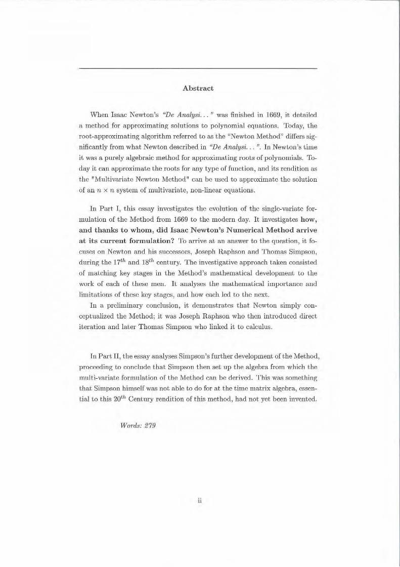
Abstract

When Isaac Newton's "De Analysi ... " was finished in 1669, it detailed

a method for approximating solutions to polynomial equations. Today, the

root-approximating algorithm referred to as the "Newton Method" differs sig­

nificantly from what Newton described in "De Analysi . . . ". In Newton's time

it was a purely algebraic method for approximating roots of polynomials. To­

day it can approximate the roots for any type of function, and its rendit ion as

the 11 Multivariate Newton Method 11 can be used to approximate the solution

of an n x n syst em of multivariate, non-linear equations.

In Part I , this essay investigates the evolution of the single-variate for­

mulation of the Method from 1669 to the modern day. It investigates how,

and thanks to whom 1 did Isaac Newton's Numerical Method arrive

at its current formulation? To arrive at an answer to the question, it fo­

cuses on Newton and his successors, Joseph Raphson and Thomas Simpson,

during the 17th and 18th century. The investigative approach taken consisted

of matching key stages in the Method's mathematical development to the

work of each of these men. It analyses the mathematical importance and

limitations of these key stages , and how each led to the next.

In a preliminary conclusion, it demonstrates that Newton simply con­

ceptualized the Method; it was Joseph Raphson who then introduced direct

iteration and later Thomas Simpson who linked it to calculus .

In Part II, the essay analyses Simpson 's further development of the Method,

proceeding to conclude that Simpson then set up the algebra from which the

multi-variate formulation of the Method can be derived. This was something

that Simpson himself was not able to do for at the time matrix algebra, essen­

tial to this 20th Century rendition of this method, had not yet been invented.

Words: 219

11

Contents

Abstract

1 Introduction

I Single-Variate Formulation

2 The Newton Method Today

3 Isaac Newton's Work

4 Joseph Raphson's Work

5 Thomas Simpson's Work

6 Preliminary Conclusion

II Multi-Variate Formulation

7 Simpson's Breakthrough

8 The Multivariate Newton Method

9 Conclusion

10 Bibliography

A Appendix

ill

ll

1

2

2

5

10

13

16

17

17

21

24

25

26

1 Introduction

Newton's Numerical Method can be referred to as an iterative algorithm that

employs differential calculus to arrive at successively closer approximations

to the root of a function . Despite being named after Isaac Newton, a brief

glance through Newton's "De analysi per aequationes numero terminorum

infinitas "1 (The analysis of Equations of Infinite Terms), where Newton first

demonstrated h.is Method, will reveal that the Method he detailed was very

different from what we today know as the Newton Method. This indicates

that ~it must have undergone substantial change since Newton's work in

''De Analysi ... ".

This essay aims to clarify the road that the Method took from the 17th

Century to the modern day. A road that is unknown even to many that.

use the Method every day. Understanding the Method 's evolution can pro­

vide an understanding of its roots and the key stages which contributed to

its development. Furthermore, this understanding can clarify who deserves

what credit for the method's effectiveness today. In short; how, and thanks

to whom, did Isaac Newton's Numerical Method arrive at its cur­

rent formulation? To answer this question it is crucial to understand the

Method's contemporary formulation and compare it to what Newton detailed

in his "De Analysi . .. 11• Once this contrast is established, it is then possible

to fill in the gaps and trace how the work of Newton's successors contributed

bo the Method's evolution.

1 Newton, 1669 (p. 218-223)

1

Part I

Single-Variate Formulation

2 The Newton Method Today

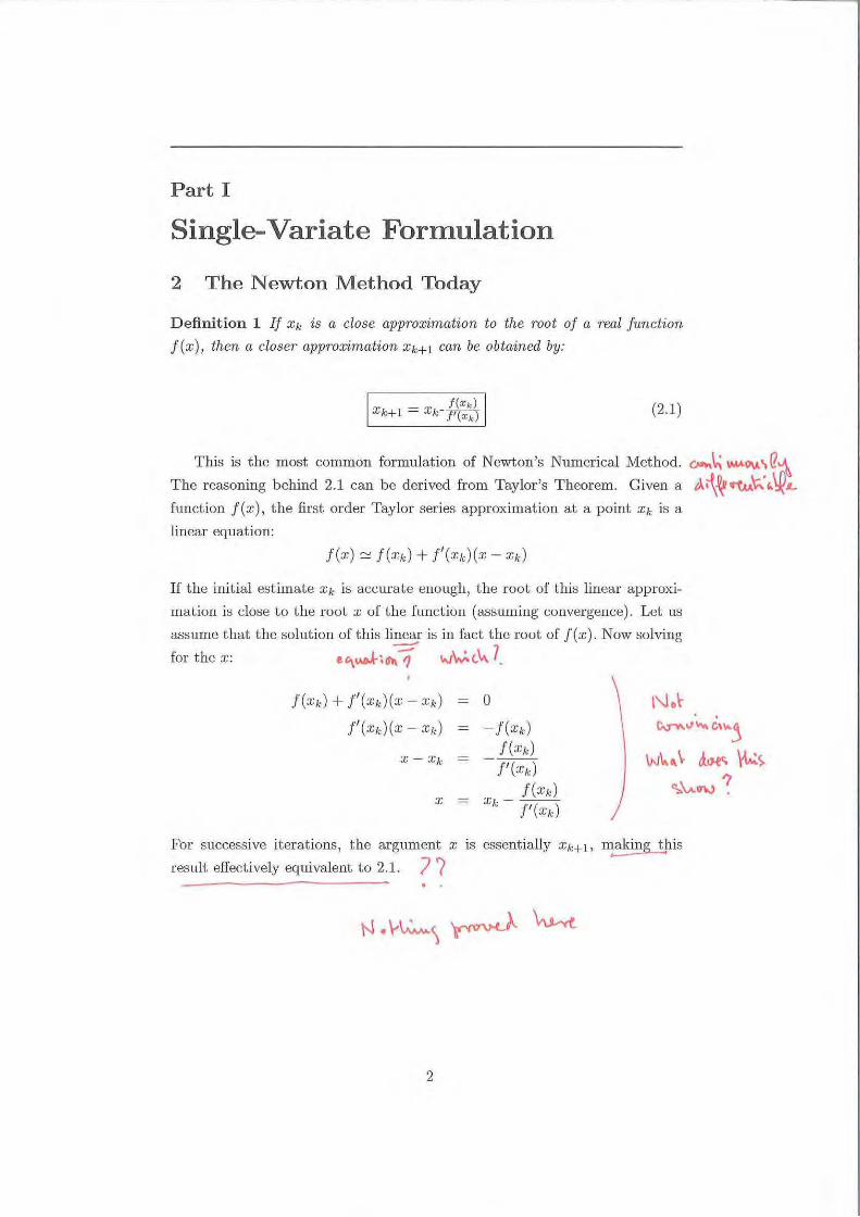
Definition 1 If Xk is a close approximation to the root of a real .function

f( x), then a closer approximation Xk+l can be obtained by:

(2.1)

This is the most common formulation of Newton's Numerical Method. D:ln~ \MA~~Q~ The reasoning behind 2.1 can be derived from Taylor's Theorem. Given a tA~~ lftu~ "\!!"­function f(x), t he first order Taylor series approximation at a point xk is a

linear equation:

If the initial estimate Xk is accurate enough , the root of this linear approxi­

mation is close to the root x of the function (assuming convergence). Let us

ass ume that the solution of this linear is in fact the root of f (x) . Now solving

for the x: '-"'.v.!M-~a'rl.-{ ~AJ'v.J..c.'v... 7_

0 . f(xA,) + f' (xk)(x - :z;k)

f' (xk)(x - xk) - f(xk ) f (xk)

~"'""'c'""j

X =

---f'(xk)

f(xk) Xk--­

f' (xk)

w\..,~ £i~t. ~>

~~""?

For successive iterations, the argument x is essentially Xk+l, ~aking tpis

result effectively equivalent to 2.1. / (

2

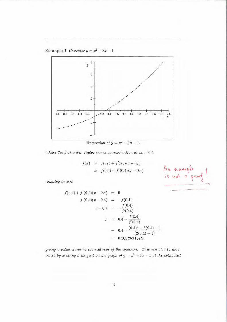
Example 1 Consider 11 = x 2 + 3x- 1

8 y

6

4

2

-1.0 -0.8 -0.6 -0.4

Illustration of y = x2 + 3x - 1.

taking the fir-st order Taylor- ser-ies appmximation at Xk = 0.4

.f(x) .f(xk) + J'(xk)(x- xk)

.f(0.4) + f'(0.4)(x - 0.4)

equating to zem

!(0.4) + J'(0.4)(x- 0.4)

f'(0.4)(x- 0.4)

X- 0.4

X

0

- !(0.4) .f (0.4)

!'(0.4) .f(0.4)

0.4- !'(0.4)

= 0 4- (0.4)2 + 3(0.4) - 1 . (2(0.4) + 3)

0.305 263157 9

2.0 X

giving a value closer to the real mot of the eq•aat·ion. This can also be illus­

tmted by drawing a tangent on the graph of y = x 2 + 3x - 1 at the estimated

3

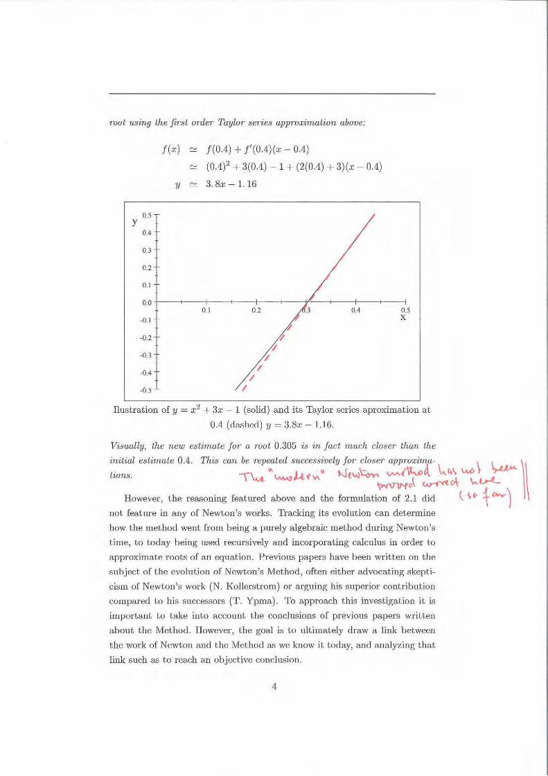
root using the first order Taylor series approximation above:

f(x) f(0.4) + f'(0.4)(x- 0.4)

(0.4? + 3(0.4) - 1 + (2(0.4) + 3)(x - 0.4)

y 3. 8x - 1. 16

0.5 y

0.4

0.3

0.2

0.1

0.0 0.1 0.2 .3 0.4 0.5

-0.1 I X

~ -0.2 ~

'/ -0.3 '/

-0.4 I

I -0.5 I

IlusLration of y = x2 + 3x- 1 (solid) and its Taylor series aproximation at

0.4 (dashed) y = 3.8x- 1.16.

Visually, the new estimate for- a root 0.305 is in fa,ct much closer· than the

·initial estimate 0.4. This can be repeated S7tccess·i·uel1J for· closer- appr-oxima- ~ ~ \\

tions. \~ "\,.,.wUtV\" Nt'-'l~ VoA.-{~~ \...~ ~~ ~c\ (J..r"(Yt ~.,

However, the reasoning featured above and the formulation of 2.1 did ( S 11 t """""J not feature in any of Newton's works. Tracking its evolution can determine

how the method went from being a purely a lgebraic method during Newton's

time, to today being used recursively and incorporating calculus in order to

approximate roots of an equation. Previous papers have been written on the

subject of the evolution of Newton's Method, often either advocating skepti-

cism of Newton's work (N. Kollerstrom) or arguing his superior contribution

compared to his successors (T. Ypma) . To approach this investigation it is

important to take into account the conclusions of previous papers written

about the Method. However , the goal is to ultimately draw a link b etween

the work of Newton and the Method as we know it today, and analyzing that

link such as to reach an objective conclusion.

4

3 Isaac Newton's Work

Conceptualization

The earliest printed accotmt of Isaac Newton 's (1642 - 1727) work on

The Method is in John Wallis' "A Treatise ... " of 1685.2 Newton 's own text

developing t he method ( "De Analysi ... ")was only published later by William

J ones.3 In spite of this, his method was known to various mathematicians at

the time, mainly through circulations of copies of his manuscripts.

Newton took an algebraic approach to the problem of approximating roots

to a function. He also credited the work of Viete as an inspiration for this

method4 ;

Definition 2 For any f(x) where X is a real root and z is a close appm:~.:­

imation, z + p is a closer approx·im ation5 . Solving for p and repeating joT

success-ively intmduced variables will give consecutive "adjustments" to the

initial estimate such that z + p + q + T + . . . will 1·esult in an ever closer

appmximation to X.

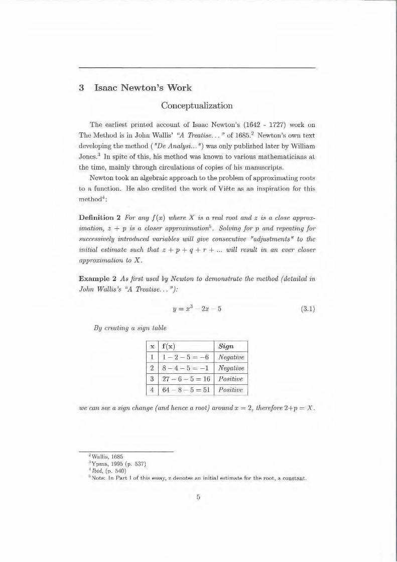
Example 2 As first ttsed by N ewton to demonstmte the method (detailed in

John Wallis 's "A Treatise . .. "):

y = x3 - 2:c- 5 (3 .1)

By cr-eating a sign table

X f(x) Sign

1 1-2-5 = -6 Negative

2 8-4-5 = - 1 Negative

3 27-6 - 5 = 16 Positive

4 64- 8 - 5 =51 Positive

we can see a sign change (and hence a root) around x = 2, the-refore 2+p = X.

2 Wallis, 1685 "1Ypma, 1995 (p. 537) I Jbid, (p. 540) "N ote: l n Part 1 of this essay, z denotes an initial estimate for the root, a constant

5

Hence:

x3 - 2x - 5 0

X = 2+p

=? (2+pY3 - 2(2+p) -5 = 0

p3 + 6p2 + lOp- 1 0 (3.2)

The two terms p3 and 6p2 can be ignored as p has such a small absolute

value that when squared and cubed it becomes insignificant to the equation.

Hence:

lOp- 1 0

p 0.1

Newton then contin'ued uS'ing the same logic, intmducing a new variable at

each iteration:

p3 + 6ri + 1 Op - 1 0

p 0.1 + q

=? (0.1 + q)3 + 6(0.1 + q)2 + 10(0.1 + q)- 1 = 0 (3.3)

q3 + 6.3q2 + 11.23q + .061 0

Again ignoring the cubic and quadmtic terms:

11.23q + .061

q

0

- 0·061 = -0.0054

11 .23

6

Iterating once moTe:

q3 + 6.3q2 + 11.23q + .061 = 0

q - -0.0054 + r (3.4)

(3.5)

====} ( -0.0054 + r)3 + 6.3( - 0.0054 + r)2+ (3.6)

+ 11.23( -0.0054 + r) + .061 0

r 3 + 6.2838r2 + 11.162r + 0.000541551 0 (3.7)

11.162r + 0.000541551 0

-0.00004852 r

The method can be continued joT as many ·iter-ations ns desir·ed. However·, it

·is evident that the method uses little more than polynomial manipulation and

continuous summation to appm~r;imate the mot. The final ste]J is to smn all

of the variables together to get the total offset from the initial estimation:

X z+p+q+r

- 2 + 0.1 - 0.0054- 0.00004852

2.09455148

. ·. X 2.09455148

(3.8)

(3.9)

This is correct to eight decimal places (for r, the last substituted variable,

has eight decimal place~:>). The rate of convergence of Newton 's method is

a rather complex theme, and outside the scope of this essay. However, let

ns go under the assumption that, despite the suggestions of Myron Pawlcy6 , ~

Maseres was right in saying that if "one step of the Newton Method is right

to n decimal places, then the next ste]J w-ill be right to 2n" _7 T his suggests

quadratic convergence (i.e. the number of correct decimal places doubles with

each iteration).

One can now begin to understand that the method originally employed

by Isaac Newton bears little resemblance with what is today known as the

"Newton Method". Firstly, it is not directly iterative. There is no recursive

0 Pawlcy, 1940 (p.l13) j [bid. (p. 114)

7

formula into which one reintroduces the approximation that was retrieved in

the last iteration. Instead, a new expression must be formulated ([3.2], [3.3],

[3.7]) in different variables every time we wish to iterate and then sum the

value of these variables must be taken at t he end [3.9]. Furthermore, there

is absolutely no connection between the method and Newton's (<Method of

Fluxions", or today's differential calculus. These two main differences were

highlighted by Nick Kollerstromti as the primary indicators that there were

more important contributions to the method later on.

It is important to note that this method works wjth polynomials, but it is

impossible to apply to non-polynomial equations without the implementation

of other mathematical tools. Nonetheless, it wa.s this formulation t hat was

developed by Isaac Newton. It constituted the first step in this long journey

of mathematical development. Despite its limitations, detailed below, it was

still of some usc at the time, and t he start of the Method's development

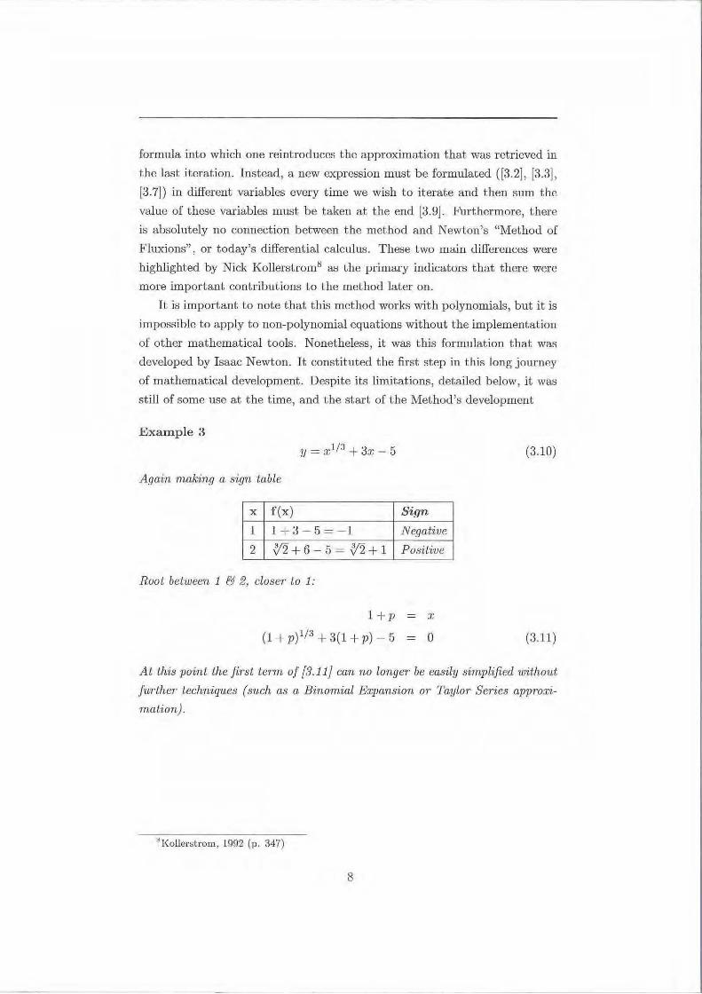
Example 3

y = x1 13 + 3x - 5

Again making a sign table

X f(x)

1 1+3-5 = -1

2 {12+6 -5 = ;/'2+ 1

Root between 1 & 2, closer to 1:

l+p

( 1 + p) 113 + 3 ( 1 + p) - 5

(3 .10)

Sign

Negative

Positive

X

0 (3.11)

At this point the first term of {3.1 1 J can no longer be easily simplified without

further techniques (such as a Binomial E:L71ansion oT TayloT Series appmxi­

rnation).

~ l<ollerstrom, 1992 (p. 347)

8

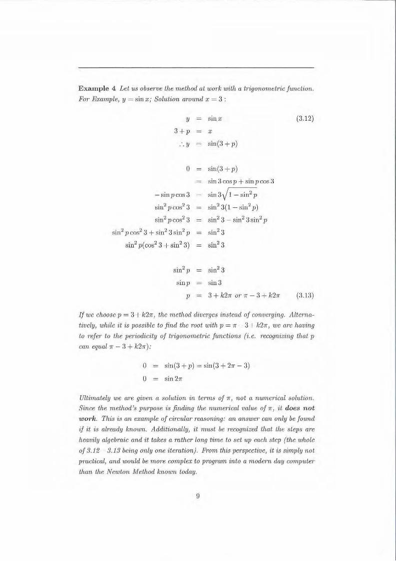
Example 4 Let •us observe the method at work with a tr··igonometric function.

For Example, y = sin x; Solution around x = 3 :

y

3+p

... y

0

- sinpcos 3

sin2 p cos2 3

sin2 pcos2 3

srnx

X

= sin(3 + p)

sin(3 + p)

sin 3 cos p + sin p cos 3

sin3J1 - sin2 p

sin2 3(1 - sin2 p)

sin2 3 - sin2 3 sin2 p

sin2 pcos2 3+sin2 3sin2 p = s in2 3

sin2 p(cos2 3 + sin2 3) sin2 3

sin2 p sin 2 3

sinp - sin3

p 3 + k27f OT 7f - 3 + k27r

(3.12)

(3.13)

If we choose p = 3 + k27r 1 the method diver-ges instead of converging. Alterna­

tively, while it is possible to find the root with p = 7f - 3 + k27r 1 we aTe having

l.o ·refeT to /,he ]Jeriodidty of trigonornetTic functions (i.e. recogn·izing that 1'

can eq'IJ.al 1r - 3 + k21f):

0 - sin(3 + p) = sin(3 + 27r- 3)

0 sin 21f

Ultimately we ar-e given a solution in te·rrns of 1r, not a nwnerical sol-ution.

S ·ince the method 's puTpose is finding the n1tmerical val1w of 1r, ·it does not

work. This is an example of circv.lar reasoning: an answer can only be found

~f 'it ·is al•ready known. Additionally, it m'ltst be re-Cognized that the 8leps ar-e

heavily algebraic and it takes a rather- long time to set up each step (the whole

of 3.12 - 3.13 being only one iteration). Prom this perspective, it is simply nol

pmctical, and would be mor-e comple.'E to pmgram into a 1node·rn day computer­

than the Newton Method known today.

9

4 Joseph Raphson's Work

Direct Iteration

Direct Iteration was introduced into the method by Joseph Raphson (1648

- 1715) . Although he published his work before Newton (1697), his work could

have been inspired by Newton 's unpublished work. Regardless, Raphson pub­

lished his "Analysis ... "9 with an almost insignificant reference to Newton,

and without any definite credit of having based his method on his contem­

porary's work10 . Raphson's method for finding the roots of equations bears

its similarities to Newton's , but makes a very important b reakthrough; it is

directly iterative.

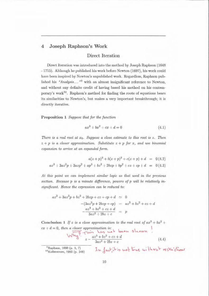
Proposition 1 Suppose that for the function

ax3 + bx2 + ex + d = 0 (4. 1)

There is a real root at xo. Suppose a close estimate to this root is z . Then

z + p ·is a closer appro:;;imation. Snbstitute z + p for x, and use binomial

e:.Dpansion to arrive at an expanded form.

a(z +p)3 +b(z+p)2 +c(z +p)+d = 0 (4.2)

az3 + 3az2p + 3azp2 + ap3 + bz 2 + 2bzp + bp2 + cz + cp + d 0 ( 4.3)

At this point u;e can implement similar logic as that 'IJ,Sed in the pr-evious

section. B ecause p is a minute difference, power-s of p will be r-elatively in­

significant. Hence the expression can be r-educed to:

az3 + 3az2 p + bz 2 + 2bzp + cz + cp + d

-(3az2p + 2bzp + cp)

az3 + bz2 + cz + d

3az2 + 2bz + c

0

a.z 3 + bz2 + cz + d

p

Conclusion 1 If z ·is a close approximation to the real root of ax3 + bx2 + c;c + d = 0, then a closer approximation is:

1 1 ~ --(~ ~t,4S '-" ~ ~4-'-' ~\A..ew\1\

'v-l"'d ?. az3 + bz2 + cz + d z - ----,------

3az2 + 2bz + c

9 Raphsou, 1690 (p. 5, 7) 1°Kollerstrom, 1992 (p. 348)

10

\

(4.4)

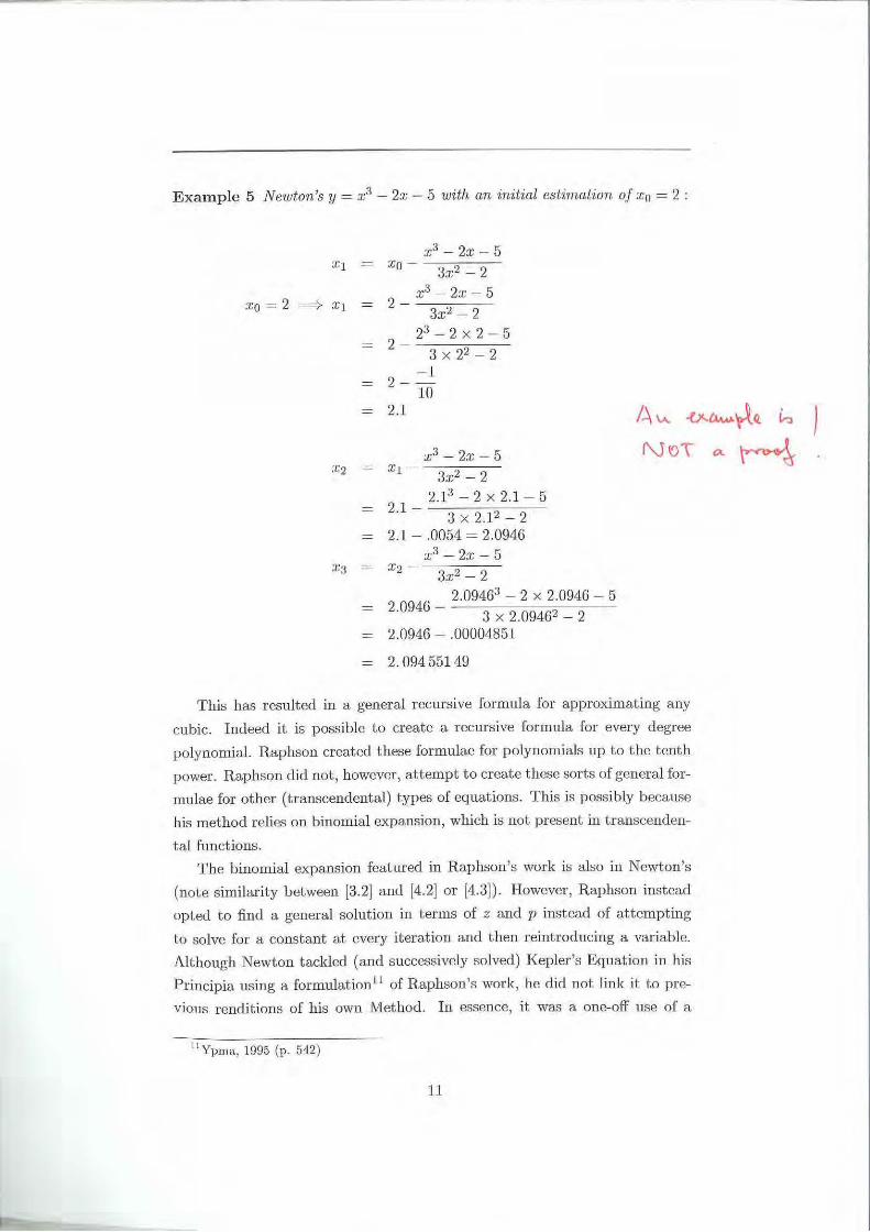
Example 5 Newton's y = x3 - 2:c - 5 with an init·ial estimation of x0 = 2 :

X Q = 2 ===> X i

x3 - 2x- 5 xo- 3x2- 2

2 _ x3 - 2x - 5

3x2 - 2

23 - 2 X 2-5 = 2 - 3 X 22 -2

- 1 2--

10 2.1

x 3 - 2x- 5 x l -

3x2- 2 2. 13 - 2 X 2.1- 5

2.1- ----=---3 x2.12 -2

2.1 - .0054 = 2.0946 x3 - 2x- 5

.'1.:2-3x2 - 2

2_0946

_ 2.09463 - 2 X 2.0946- 5

3 X 2.09462 - 2 = 2.0946- .00004851

2. 094 55149

This has resulted in a general recursive formula for approximating any

cubic. Indeed it is possible to create a recmsive formula for every degree

polynomial. R aphson created these formulae for polynomials up Lo the tenth

power. R aphson did not, however, attempt to create these sorts of general for­

mulae for other (transcendental) types of equations. This is possibly because

his method relies on binomial expansion, which is not present in transcenden­

tal functions.

The binomial expansion featured in Raphson's work is also in Newton 's

(note similarity between [3.2] and [4.2] or [4.3]). However, Raphson instead

opted to find a general solution in terms of z and p instead of attempting

to solve for a constant at every iteration and then reintroducing a variable.

Although Newton tackled (and successively solved) Kepler's Equation in his

Principia using a formulation 11 of Raphson's work, he did not link it to pre­

vious renditions of his own Method. In essence, it was a one-off use of a

l l Yprn a, 1995 (p. 542)

11

particular approach to a problem, and not the formulation of a method for

iteratively approximating roots (something only Raphson was able to do). __ 7

connection between the numerator and the denom­

inator in [4.4]. The a ter is the deri.vc1t ive of the former. This was, however,

a connection that was not made until many years later by Joseph Simpson.

An a ttempted explanation as to why Raphson did not spot the calculus in

the method is that many of the calculus developments of the 1690s (When

Raphson worked on this met hod) were made in mainland Europe whereas

Rapbson was in England. Perhaps the reference of 1690s Leibnizian calculus

developments w&; De L'Hopital's "Analyse d'Infiniments Petits", published

in 169612 . This work certainly contained the required calculus to draw re­

semblance between the algebra employed by Raphson in his Method and

Differential Calculus. However , it seems as though Raphson was completely

unaware of it; his only calculus reference being Newton's work featured in J.

Wallis' Opera Ma.thernatica of 1693, it was insufficient to link the two fields

of algebra and differential calculus in this particular method.13

It must be noted that as mentioned by Kollerstrom14 , Rapbson was not

the only English mathematician who failed to appreciate Leibniz's calculus;

Edmond Halley too failed to link his algebraic method to ftUA'ions. This is

probably due to the fact t hat "new ideas take a while to become accepted" 15 .

Even years later when Simpnon drew the connection between the algebra of

the method and differential calculus, some might have argued that it was so

revolutionary that it might be wrong to connect the two fields so directly.

It is essential to analyze the importance of his method from a recursive

perspective; it is now much easier to perform successive iterations and arrive

at a root t o the polynomial.

12Ypma, 1994. ( p. 543 ) 1 ~Koll erstrom , 1992 (p. 349) 11 Ibid. (p. 350) if> Ibid (p. 349)

12

5 Thomas Simpson's Work

The Introduction of Calculus

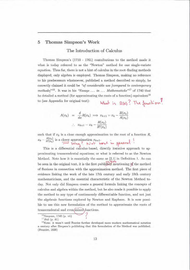
T homas Simpson's (1710- 1761) contributions to the method made it

what is t oday referred to as the "Newton" method for one single-variate

equation. Thus far , there is not a hint of calculus in the root- finding methods

displayed ; only algebra is employed . Thomas Simpson, making no reference

to his predecessors whatsoever, published a method described so simply, he

correctly claimed it could be "of considerable use (compared to contemporary

methodsj"16 . It was in his "Essays ... in .. . Mathematicks"17 of 1740 that

he detailed a method {for approximating the roo ts of a function) equivalent18

to (see Appendix for original text): W'-"'~ ;c:, R.(;;c.) ( 1~ ~c\i.: f:1YI 7

such that if Xfc is a close enough approximation to Lhe root of a function R, R(xk . 1 . t ' \ Xk - R' (xk IS a c oser apprmama ·wn :ck+ 1- ~ 0

-;:=:! \N~ 1. No\- ~~l.. '- ~'rtA.-\. ·

This is a differential calculus-based, d irectly iterative approach to ap­

proximating transcendental equations; or what is referred to as the Newton

Metlwd. Note how it is essentially the same as r2.1] in Definition 1. As can \\cr..

be seen in the original text, it is the first publi~d mentioning 9<£ the method

of fluxions in connection with the approximation method. The first piece of

evidence linking the work of the late 17th century and early 18th century

mathematicians, and the essential characteristic of t he Newton Method to­

day. Not only did Simpson create a general formula linking the concepts of

calculus and algebra within the m ethod, but he also made it possible to apply

the method to any type of continuously differentiable function, and not just

t he algebraic functions explored by Newton and Raphson. It is now possi­

ble to use this new formulation of the method to approximate the roots of

transcendental and evene funct.ions.

11;Simpson, 1740 (p. vii) ? 17 Jbid (p. 81) I

JXNotc: il; wasn't; unti1 Fomier iiuther developed more modern mathematical notation a centw·y after Simpson's publishing that this formulation of the Method was published. (Fourricr, 1830)

13

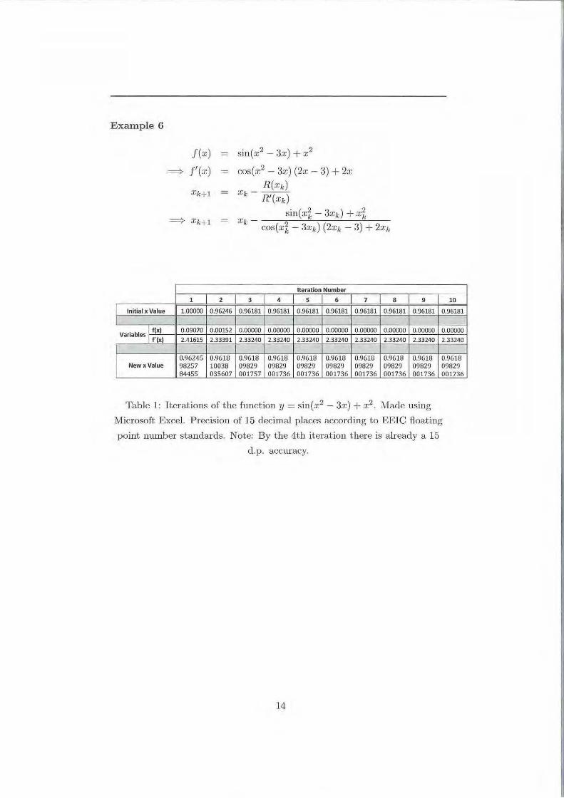
Example 6

Initial x Value

. I f(x) Vanables J f'(x)

New x Value

f (x) ===} f' (x)

=

1 2

1.00000 0 .96246

0.09070 0.00152

2.41615 2.33391

0.96245 0.9618 98257 10038 84455 035607

sin (;.c? - 3x) + x2

cos(x2- 3x) (2x- 3) + 2x

R(e!:,,J X!c- R'(x~c)

.. sin(x~- 3xk ) + xz Xk - cos(xz - 3xk ) (2x"' - 3) + 2xk

Iteration Number

3 4 5 6 7 8

0.96181 0.96181 0.96181 0.96181 0.96181 0.96181

0.00000 0.00000 0.00000 0.00000 0.00000 0.00000

2.33240 2.33240 2.33240 2.33240 2.33240 2.33240

0.9618 0.9618 0.9618 0.9618 0.9618 0.9618 09829 09829 09829 09829 09829 09829 0017':)7 001736 001736 001736 001736 001736

9 10

0.96181 0.96181

0 .00000 0.00000

2.33240 2.33240

0.9618 0.9618 0 9829 09829 001736 001736

Table 1: Iterations of the function y = sin(x2 - 3x) + x 2. Made using

Microsoft Excel. Precision of 15 decimal places according to EEIC floating

point number standards. Note: By the 4th iteration there is already a 15

d. P- accuracy.

14

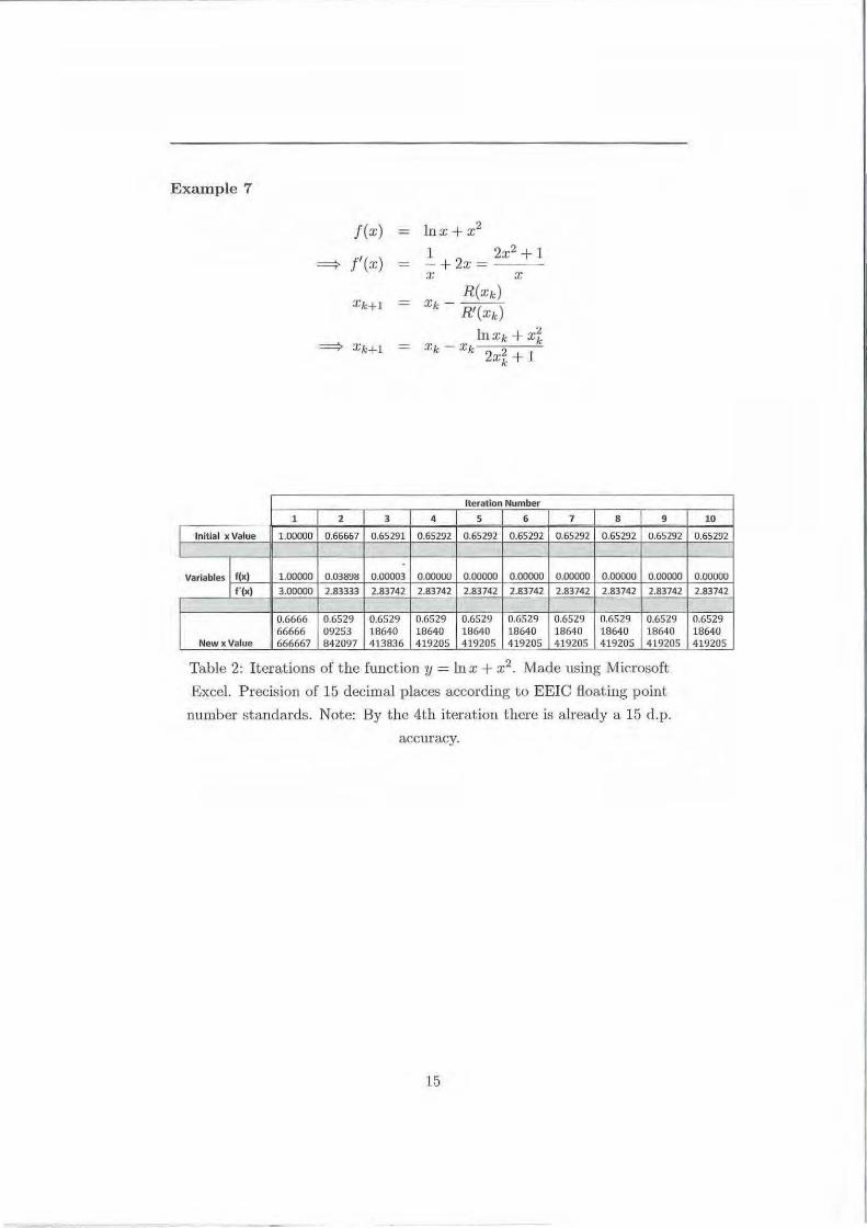
Example 7

1

Init ial x Value 1.00000

Variables I f(x) 1.00000

I f '(x) 3.00000

0.6666 66666

New xValue 666667

f (x)

=> f' (:x:)

=

=

2 3

0.66667 0.65291

0.03898 0.00003

2.83333 2.83742

0.6529 0.6529 09253 18640 842097 41 3836

ln x + x2

1 2

. _ 2x2 + 1 -+ :r,- - --x X

R(xk) X~c - --­

R'(xk) ln :c~c + x%

Xk- Xk 2 2xk + 1

Iteration Number

4 5 6

0.65292 0.65192 0.65292

0.00000 0.00000 0.00000

2.83742 2.83742 2.83742

0.6529 0.6529 0.6529 18640 18640 18640 419205 419205 419205

7 8 9

0.65192 0.65192 0.65292

0.00000 0.00000 0.00000

2.83742 2.83742 2.83742

0.6529 0.6529 0.6529 18640 18640 18640 419205 419205 419205

Table 2: Iterations of the function y = ln x + x2. Made using Microsoft

Excel. Precis ion of 15 decimal p laces according to EEIC .floating point

number standards. Note: By t he 4th iteration there is a lready a 15 d.p.

acCIIracy.

15

10

0.65292

0.00000

2.83742

0.6529 18640 419205

6 Preliminary Conclusion

Thus far it can be concluded that the Newton method , while bearing t he

name of only one of its contributors , was the result of the efforts of multiple

men. It was thanks to Isaac Newton that the method was first conceived,

but in its crude shape it was of little use compared to the recursive definit ion

demonstrated by Raphson. E ven so, it was not Lmtil Simpson introduced

calculus that t he method was truly of gTeat use fOT approximating the roots

of all types of functions. Interestingly, Newton was the only man who divulged

where the inspiration for his method came from. The other two men failed

to acknowledge any links between their methods mathematics of their peers,

suggesting they either came up with their methods themselves or where not

inclined to credit their predecessors

The reason for Newton's name being associated with the Method is prob­

a bly due t o the fact that when leading mathematicians like Joseph Louis La­

grange (1736- 1813) and Jean Baptist e .Joseph Fourrier (1768- 1830) wrote

their papers over half a century later, formulating the modern mathematical

notat ion of the Method, t hey referred t o it by Newton's name, never refer­

encing t he other contributors.1!J With regards to the work of Lagrange and

Fourrier, it did not contribute t o the method as much as it contributed to

mathematics itself, and the method inherent ly benefitted from these develop­

ments. However , at its cor e, and in terms of its efficiency, it did not change,

it was simply reformulated. While these men 's contributions to the Method

must not b e overlooked, they were secondary to the work of the aforemen­

tioned others, and hence beyond the scope of this essay. Nonetheless, the

influential weight of these two men and their publications amongst the scien­

tific world sheds some light as to why today we usually credit Newton alone

for t his method's development.

(~\- ~ 'w.w4. ~,.vo\ ~~ ~kt C::rr.~ ~· ~ :> - ~~ ~ Y\.ul. VJ tJ~ ~

19Cajori , 1911 (p. 29-32)

16

Part II

Multi-Variate Formulation

7 Simpson's Breakthrough

Extending the Investigation

Despite having formulated a partial conclus ion for the initial question,

and having described the evolution of the method to its formulation [2.1]. this

conclusion is potentially incomplete. To understand why, further analysis of

Thomas Simpson's work is required. Although we have explained the evolu­

tion of the method's singlevariate formulation, Simpson's work hints towards

another formulation of the method which was not particularly significant in

it time, but evolved to much greater importance in t he 20th Century. This

would become a multivariate version of [2.1], today known as the Multivariate

Newton Method.

2 Equations in 2 Variables

Simpson 's "Essays . ... " 20 was a significant publication for the development

of the Newton Method as we know it. His "Case I", as detailed above, handles

the root-approximation of single non-linear equations in one variable. Simp­

son did not, however, stop at this point; he proceeded to describe a similar

method for the approximation of the intersection of 2 implicit functions in 2

variables. Albeit more complex, it too is a significant achievement - not on

its own, but for the questions it r-aises and the path it leads to.

Simpson made no reference as to where he might have discovered inspira­

tion for this particular method, and leaves the reader to presume he intuitively

followed it tlu·ough from his "Case I". The definition below is interpreted us­

ing modern mathematical notation from Simpson's own work. (See Appendix

for original text).

20 Simpson, 1740 (p. 82)

17

Definition 3 Take the partial 'lerivatives with respect to each variable of the

two functions to be approximated. Giving them a variable name, "A" repre­

sents the partial derivative of h with 1·espect to x. Similarly, "B" represents

the partial derivative of f1 with respect toy. Lowercase "a" and ''b " are the

same lnd for h.

[) A (7.1) - 11

ax

a f 7]-1 y B (7.2)

af -2 ax

a (7.3)

8 b (7.4) -h = ay

The final step is to combine the above variables into two ad-hoc "multiples 11

~x and ~y , to arrive at the value by wh·ich to adjust Xk and Yk, the initial

estimated coordinates of the intersection.21

Br - bR (8 Ab-aB

aR-AT G Ab-aB

where R and r are the two equations being intersected:

fl(x , y ) R

fz(x, y) r

Then, estimating initial val·ues of Xk and Yk of the intersection, the closer

values xk+l and Yk+l can be attained b1;: \N ~ ~ ~~ ~ \..u>\- S Vw"' ·

Br-bR Xk+l Xk + ~xk = :l;k + Ab- aB

aR-Ar Yk+l = Yk + ~Yk = Yk + Ab _ aB

(7 .5)

(7.6)

The great benefit of this method is allowing us to find the intersection

between two ftmctions in their implicit form. For example, in the intersection

of [7.7]and [7.8]. N 0 \.. 5\...1!> w \,. 1• '·

21 Note: Tn the Part li of this essay, subscript k denotes the argument to which the st~bscript belongs evaluated at the kth iteration.

18

--- --- ~~-~~---- ---

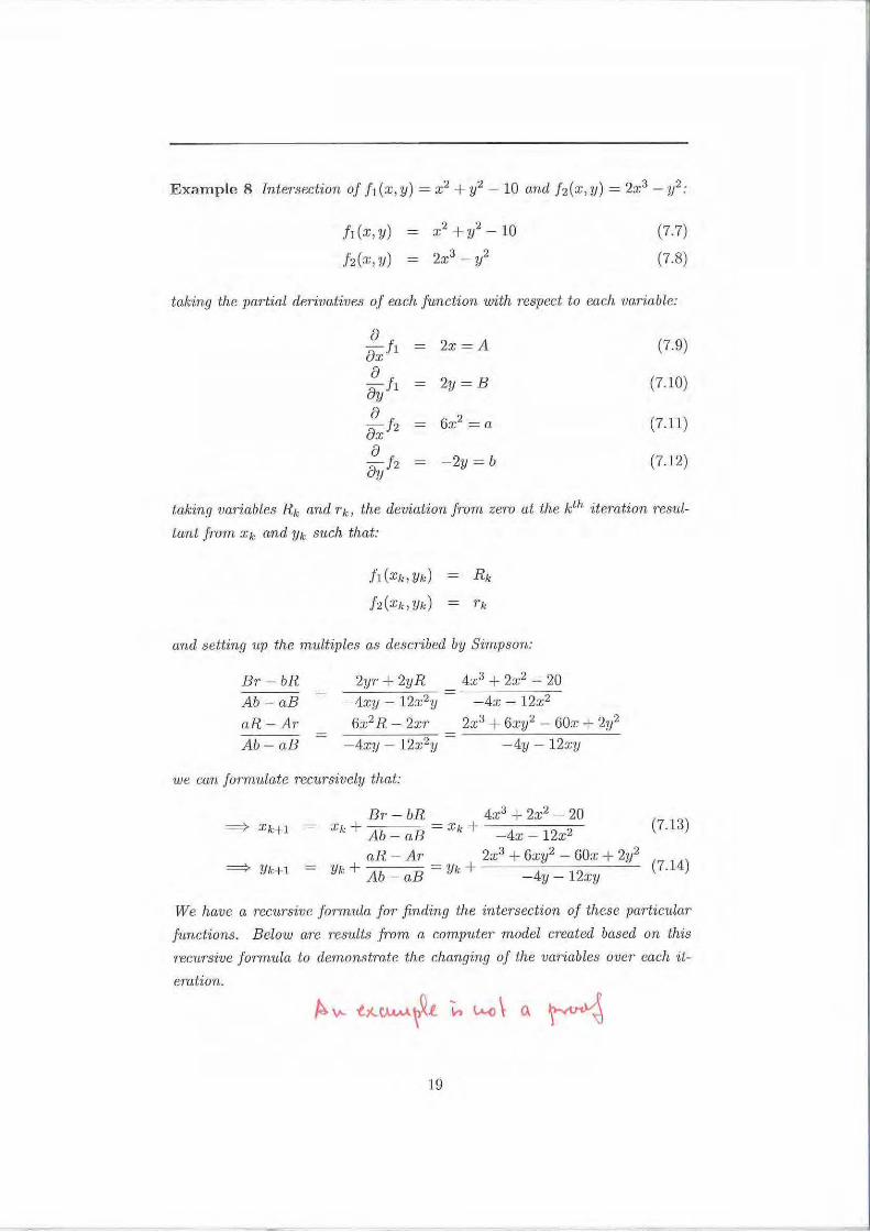
Example 8 Intersection of ,h(x,y) = x2 +y2 - 10 and h (x, y) = 2x3 -y2:

!J(x, y )

h(x, y)

2 ') X +y- - 10

2x3 - Yz

(7.7)

(7.8)

taking the partial derivatives of e(Lch function with respect to each ·variable:

a 2x=A (7.9) -!1

ax a

2y=B (7.10) -h av a

6x2 =a (7.11) - h OX a

(7.12) -h - 2y = b ay

taking variables Rk and Tk, the deviation from zem at the kth iteration resul­

tant from Xk and '!Jk such that:

h (xk, Yk) Rk

h(xk , Yk) rk

and setting up the multiples as descr~ibed by Simpson:

Br-bR Ab-aB

o.R- Ar Ab-aB

2yr· + 2yR

-4xy- 12x2y

6x2R - 2xr - 4xy- 12x2y

4x3 + 2x2 - 20 -4x- 12:c2

2x 3 + 6xy2 - 60.r. + 2y2

- 4y -12xy

we can formulate recursively that:

Br - bR 4x3 + 2x2 - 20 Xk + Ab - aB = Xk + - 4x -12x2 (7·13)

aR - Ar· 2x3 + 6xy2 - 60.'1: + 2y2

Yk + Ab B = Ylr + 4 12 (7.14) -a - y - xy

We have a recur·sive formula for finding the intersection of these particttla.r

.fnnctions. Below are r·esv.lts from a computer model created based on this

Tecursive formula to demonstrate the changing of the variables over each it­

emtion.

19

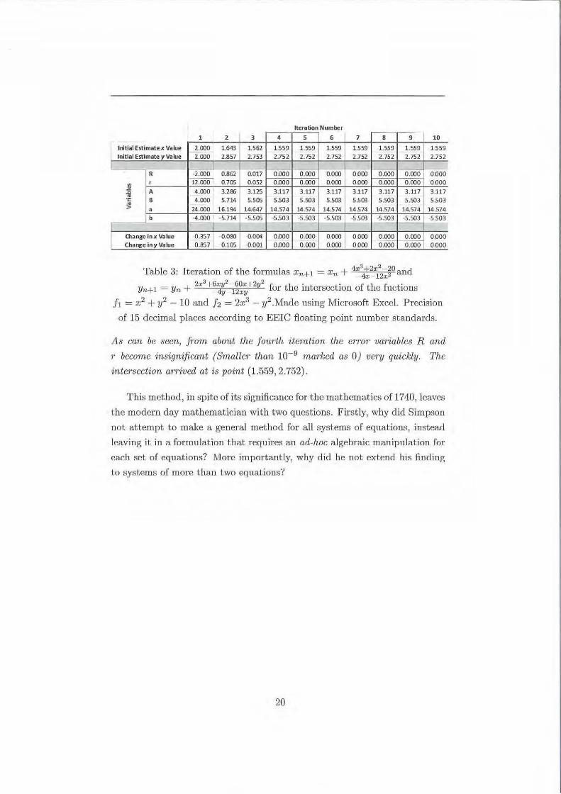
Iteration Number

1 I 2 3 4 5 6 7 r-s--1- 9 I 10

Initial Estimate x Value 2.000 1.643 1.562 1.559 1.559 1.559 1.559 1.559 1.559 1 1.559 Initial Estimate y Value 2.000 2.857 2.753 2.752 2.752 2.752 2.752 2.752 2.752 2.752

- 0:000 0 .000 R -2.000 0.862 1 0.017 0 .000 0.000 0 .000 0.000 0.000

~ r 12.00iJ 0.705 0.052 0.000 0.000 0.000 0 .000 o.ooo 0.000 0 .000

:0 A 4.000 3.286 3.125 3.117 3.117 3.117 3.117 3 .117 3.117 3.117 "' ---- --

~ 8 4.000 5.714 5.505 5.503 5.503 5.503 5503 5.503 5.503 5.503

a 24.000 16.194 14.647 14.574 14.574 14.574 14.574 14.574 14.574 14.574 b -4.000 - 5.714 -5.505 -5.503 -5.503 -5.503 -5.503 -.2;!!03 -5.~ -5.503

-

Otange in x Value -{).357 -0.080 I -0.004 0.000 0.000 0.000 I 0.000 0.000 I~ 0.000 Change in y Value 0.857 ·0.105 -0.001 0.000 0.000 0.000 0.000 0.000 0.000 0.000

rp bl 3 I . f h f l 4x3+2x2 - 20 d .~.a e : teratwn o t e ormu as Xn+ 1 = Xn + _4x _ 12x2 an 2 3 6 2 60·2 2

Yn+ 1 = Yn + X + -~~-~2x~+ y for the intersection of the ructions

/1 = :~:2 + y2 - 10 and h = 2x3

- zl.Made using Microsoft Excel. Precision

of 15 decimal places according to EEIC floating point number standards.

As can be seen, from about the fourth i/,emtion the error· ·ua.riables R and

r become insignificant (Smaller than 10- 9 marked as 0) very quickly. The

intersection mTived at is point (1.559, 2.752) .

This method, in spite of its significance for the mathematics of 1740, leaves

the modern day mathematician with two questions. Firstly, why did Simpson

not attempt to make a general method for all systems of equations, instead

leaving it in a formulation that requires an ad-hoc algebraic manipulation for

each set of equations? More importantly, why did he not extend his finding

to systems of more than two equations?

20

8 The Multivariate Newton Method

n Equations in n Variables

Thus far we have seen how Simpson not only developed the Newton

Method of today for single non-linear equations, but also for systems of two

equations in two variables. However, his impact upon the field of numericQ.l

analysis went deeper, and can still be seen today. It led to a method for

solving n functions in n variables. To illustrate this, let us employ a tool

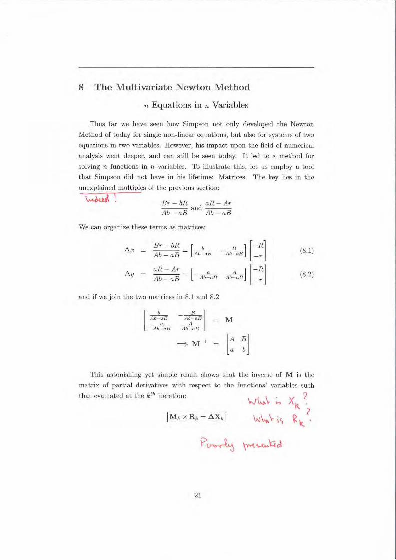
that Simpson did not have in his lifetime: Matrices. The key lies in the

unexplained multiples of the previous section:

'\M.~u.J. ~ Br- - bR aR - A-r ---- and - --­Ab - aB Ab - aB

We can organize these terms as matrices:

flT-bR [ --,-,--=-- b Ab - aB - Ab-aB

aR- Ar- [ Au - oB = - llb~aR

and if we join the two matrices in 8.1 and 8.2

[_Ab~:.R Ab-a.I3

- /\~l!.cL8 ] Ab-alJ

llb~nB]

M

(8.1)

(8.2)

This astonishing yet simple result shows that the inverse of M is the

matrix of partial derivatives with respect to the functions' variables such

that evaluated at the kth iteration:

21

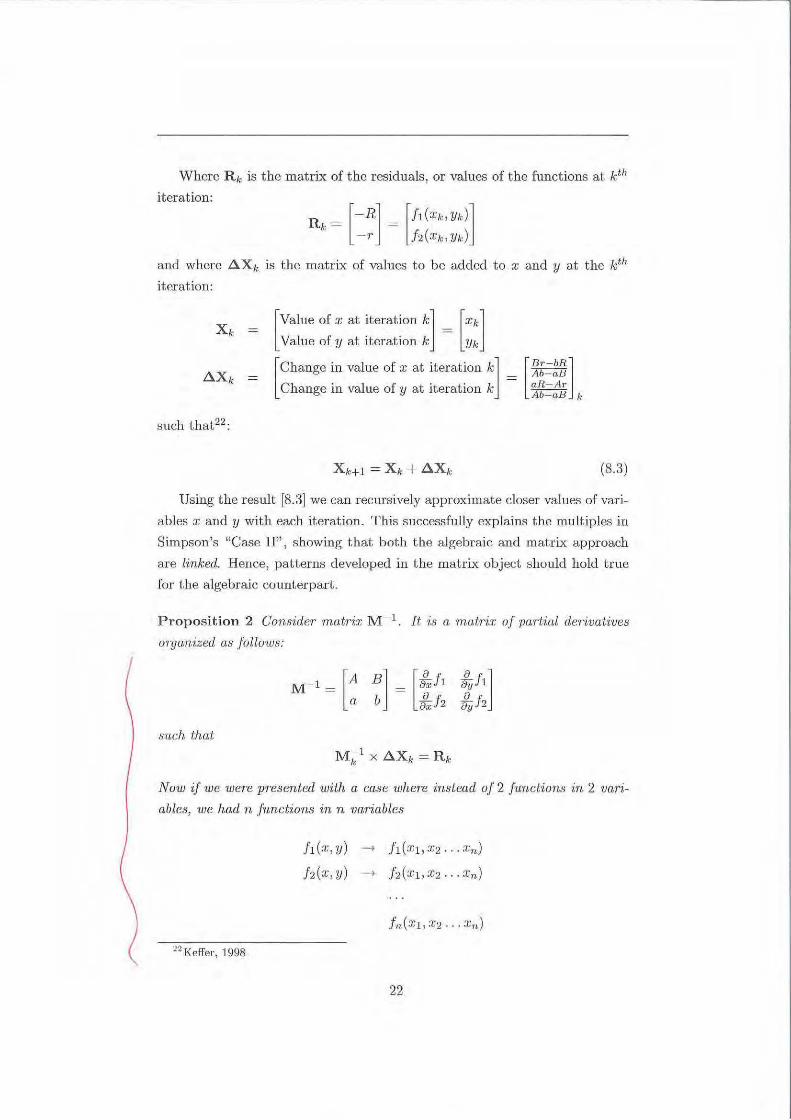
Where R 1c is the matrix of the residuals, or values of the functions at kth

iteration:

and where AX1c is t he matrix of va lues to be added to x and y at the kth

iteration:

such that22 :

[Value of x at iteration kl = [xkl Value of y at iteration k Yic

[Chango in value of x at iteration kl Change in value of y at iteration k [

BT·-bR] 1\b-aB aR- Ar Ab- aB k

(8.3)

Using the result [8.3] we can recursively approximate closer values of vari­

ables x and y with each iteration. This successfully explains the multiples in

Simpson's "Case II", showing that both the algebraic and matrix approach

are l inked. Hence, patterns developed in the matrix object should hold true

for tlle algebraic counterpart.

Proposition 2 Consider matri:r; M-1 . It is a mair'i:r; of paxl·ial derivatives

organized as .follows:

snch that

N ow ~f we were presented with a case where instead of 2 functions in 2 vari­

ables, we had n .functions in n vwriables

~2 Keffer, 1998

h (:r:, y) ~ h(x1 ,1:2 ... xn)

fz(x , y) ~ J2(xl,X2 · · ·xn)

22

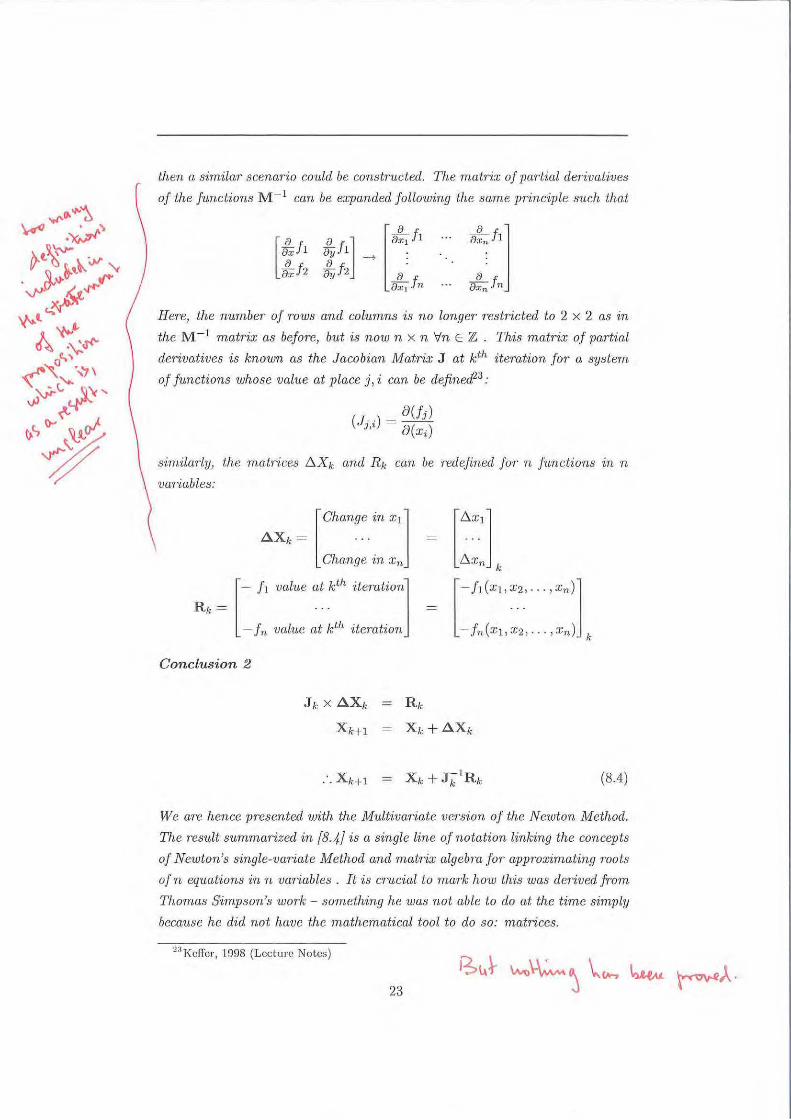
then a similar- scenario conld be constr'Ucted. The matri:~: of par-t·ial der-ivatives

of the functions M-1 can be expanded following the same pr-inciple such that

[tx.ft & j" ax 2

a~,~h ] a f. ax;: n

Here, the number of rows and col·umns is no longer restr-icted to 2 x 2 as in

the M - 1 matrix as befor-e, but is now n x n 'linE Z . This matrix of partial

derivatives is known as the Jacobian Matrix J at kth itemtion for a system

of functions whose val·ue at place j, i can be defineJ23 :

si,rnilarly, the matrices !J,.Xk and Rk can be r-edefined for- n functions in n

var-iables:

[

Change in :r;11 .6.Xk = · · ·

Change in Xn

[

- .fi value at kth iteration]

Rk = - fn val·ue ~; ~lh itemtion

Conclusion 2

(8.4)

We aTe hence pr-esented with the Multivariate veTsion of the Newton Method.

The r-esult summar-ized in [8.4] is a single line of notation linking the concepts

of Newton's single-variate Method and matrix algebra joT approximating roots

of n equations in n vaT·iables . I t ·is crucial to mark how this was derived from

Thomas S·impson's work - something he was not able to do at the time simply

because he did not have the mathematical tool to do so: matr-ices.

n Keffer , "1998 (Lecture Notes)

23

9 Conclusion

Newton 's work was critical to the development of the method - it was his

thought experiments that sparked it. Hence, to him should be attributed the

snccess of conceptualizing the method. However, we should not disregard

the work of his successors; Raphson and Simpson, who made the contem­

porary application of the method explained in Part I of th is essay possible.

It was Raphson who developed its direct iteration, and it was Simpson

who linked it with calculus making it possible for the Method to then de­

velop in the twentieth century, as shown in Part II, to approximate solutions

for systems of n equations in n variables. These four critical points

represent the four steps that the Method went through: Conceptualization ,

Development of Direct Iteration , Link with Calculus and Link with Matrices

& systems of equations. An evolution t hat took over 300 years.

However , when it comes to the Multivariate Newton Method , it was Simp­

son 's work that most significantly contributed to it. The ad-hoc multiples

were a foreshadowing of the work to come in the 20th Century, and inher­

ently the multivariate version of the algorithm should be named after the

Thomas Simpson, the man who first hinted at it , just as the Newton Method

is named after Isaac Newton.

P erhaps for tills reason , and for pragmatic purposes, the Method is rightly

named after Isaac Newton. But he was not the Method's sole father. The

method is instead the offspring of centuries of mathematical development and

holistic cooperation.

Ultimately it was not the work of one man, but the successive develop­

ment of t he method throughout the ages that makes it so useful today. This

paper does not intend to designate one rnan as t he master behind the method

(as others have before), but ins tead highlight how it was overlapping and

continuous work of all these men that contributed to the evolution of Isaac

Newton's N urnerical Method.

From an algebraic method for approximating roots of polynomials, to a

recm sive algorithm for approximating solutions of multivariate non-linear sys­

tems using matrices, this method is a story of true mathematical continuity.

T bP. knowledge cont inuum that moves science forward.

W01·ds: 3800

24

10 Bibliography

References

Cajori, F. (1911). H·istorical Note on the Newton-Raphson Method of Approx­

imation. The American Mathematical Monthly.

Encyclopmdia Britannica. (2011). flmok Taylor. Retrieved Sep-

tember 11, 2011, from Encyclopmdia Britannica Online:

www. bri tannica.com /EBchecked /topic/ 584 793 / Brook-Taylor

Fourier , J. (1830). A naly8e des Equations Determinees. Paris: Firmin Didot

Freres, Libraires.

Keffer, D. (1998). Rootfinding in systems of Equations. Knoxville, Tennes::;ee.

Kollerstrom, N. (1992, 25). Thomas Simpson and "Newton's method of ap­

proximation 11: an enduring myth. Brit ish Journal of Historical Science.

Newton, I. (1711). De analysi per aequationes n·umero terminorum ·in.fin'itas.

In D . T. Whiteside's, The Mathematical Papers of Isaac Newton . London.

Pawley, M.G. (1940). New OriteTia for Accuracy in App·roximnting Real Roots

by the Newton- Raphson Method. National Mathematics Magazine.

Raphson, J. (1690). Analysis Aequationwn Uni·ue?·sal·is. London.

Simpson, T. (1740). Essays On Several Curious And Useful Sub.fects, In Spec­

ulative And Mixed Mathematics. London.

Wallis, J. (1685). A Trwtise of Algebr-a both Historical cmd Pr-actical. London.

Yprna, T. J. (1995, December Vol. 37, No. 4). Historical Development of the

Newton-Raphson Method. Society for Industrial and Applied Mathematics

Review.

25

A Appendix

Extracts from Thomas Simpson's "Essays On Several Curious

And Useful Subjects, In Speculative And Mixed Mathematics."

Page 81:

Case I, When only one Equation is given, and one Quantity

( x) to be determined.

Take t he fluxion of the given Equation (be it what it will)

supposing x, the unlrnown, to be the variable Quantity; and hav­

ing divided the whole by xl,let the Quotient be represented by

A. Estimate the value of x pretty near t he Truth, substituting

the same in the Equation, as also in the Value of A , and let the

ErrorR, or resulting Number in the former, be divided by this

numerical Value of A, and the Quotient be sub-tracted from the

said former Value of x; and from thence wiU arise a new Value of

that Quantity much nearer to the Truth than the former, where­

with proceeding as before , another new Value may be had, and so

an-other, etc. 'till we arrive to any Degree of Accuracy desired.

Page 82:

Case II, When there arc two Equations given, and as many

Quantities (x andy) to be determined.

Take the Fluxions of both the Equations , consideringx and y

as variablc,and in the former collect all the Terms, affected with

xl , under their proper Signs, and having divided by x l , put the

Quotient A; and let the remaining Terms, divided byyl, be rep­

resented by B : In like manner, having divided the Terms in the

latter , affected with x l , by xl, let the Quotient be put = a, and

the rest, divided byyl ,= h. Assume the Values of xand y pretty

near the Truth, and substitute in both the Equations, marking the

Error in each, and let these Errors, whether positive or negative,

be signified by R and r respectively: Substitute likewise in the

l fA B b d l t (B1·-bR) d (aR-A1·~ b d . va ues o a , an e (Ab-aB) an (Ab- aB e converte mto

Numbers, and respectively added to the former Values of x and

y; and thereby new Values of those Quantities will be obtained;

from whence, by repeating the Operation, the true Values may be

approximated. ad libitum.

26