Excel -- Data Validation - Charles Darwin...
72
Excel -- Data Validation Home Excel Tips Sample Spreadsheets Excel -- Data Validation 1. Data Validation -- Introduction ● What is Data Validation? ● Provide a Drop-down List of Options ❍ Create a List of Items ❍ Name the List Range ❍ Apply the Data Validation ❍ Using a Delimited List ❍ Allow Entries that are not in the List ❍ Protect the List 2. Data Validation -- Create Dependent Lists 3. Hide Previously Used Items in a Dropdown List 4. Display Messages to the User 5. Use a List from Another Workbook 6. Validation Criteria Examples 7. Custom Validation Criteria Examples 8. Data Validation Tips 9. Data Validation Documentation 10 Data Validation -- Combo box 11. Data Validation -- Combo Box - Named Ranges Download the zipped sample workbook What is Data Validation? Data validation is a tool that helps you control the kind of information that is entered in your worksheet. With data validation, you can: --provide users with http://www.contextures.com/xlDataVal01.html (1 of 6)04/09/2006 8:11:10 PM
Transcript of Excel -- Data Validation - Charles Darwin...
Excel -- Data Validation
Home Excel Tips Sample Spreadsheets
Excel -- Data Validation
1. Data Validation -- Introduction
● What is Data Validation? ● Provide a Drop-down List
of Options ❍ Create a List of Items❍ Name the List Range❍ Apply the Data
Validation❍ Using a Delimited
List❍ Allow Entries that
are not in the List❍ Protect the List
2. Data Validation -- Create Dependent Lists3. Hide Previously Used Items in a Dropdown List4. Display Messages to the User5. Use a List from Another Workbook 6. Validation Criteria Examples 7. Custom Validation Criteria Examples8. Data Validation Tips 9. Data Validation Documentation 10 Data Validation -- Combo box 11. Data Validation -- Combo Box - Named Ranges
Download the zipped sample workbook
What is Data Validation?
Data validation is a tool that helps you control the kind of information that is entered in your worksheet. With data validation, you can:
--provide users with
http://www.contextures.com/xlDataVal01.html (1 of 6)04/09/2006 8:11:10 PM
Excel -- Data Validation
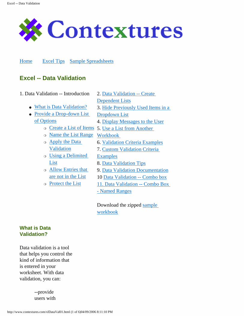
a list of choices --restrict entries to a specific type or size--create custom settings
Note: Data validation is not foolproof. It can be circumvented by pasting data into the cell, or by choosing Edit|Clear|ClearAll
Data validation list
Provide a Drop-down List of Options
Use Data Validation to create a dropdown list of options in a cell. List items can be typed in a row or column on a worksheet, or typed directly into the Data Validation dialog box.
1. Create a List of Items
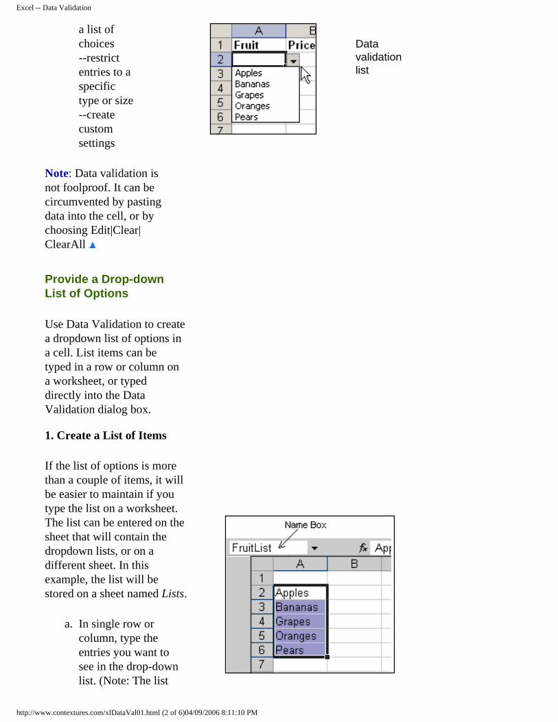
If the list of options is more than a couple of items, it will be easier to maintain if you type the list on a worksheet. The list can be entered on the sheet that will contain the dropdown lists, or on a different sheet. In this example, the list will be stored on a sheet named Lists.
a. In single row or column, type the entries you want to see in the drop-down list. (Note: The list
http://www.contextures.com/xlDataVal01.html (2 of 6)04/09/2006 8:11:10 PM
Excel -- Data Validation
must be in a single block of cells -- e.g. you can use A2:A6, but not A2, A4, A6, A8.)
2. Name the List Range
If you type the items on a worksheet, and name the range, you can refer to the list from any worksheet in the same workbook.
1. Select the cells in the list.
2. Click in the Name box, to the left of the formula bar
3. Type a one-word name for the list, e.g. FruitList.
4. Press the Enter key.
Note: To create a named list that automatically expands to include new items, use a dynamic range.
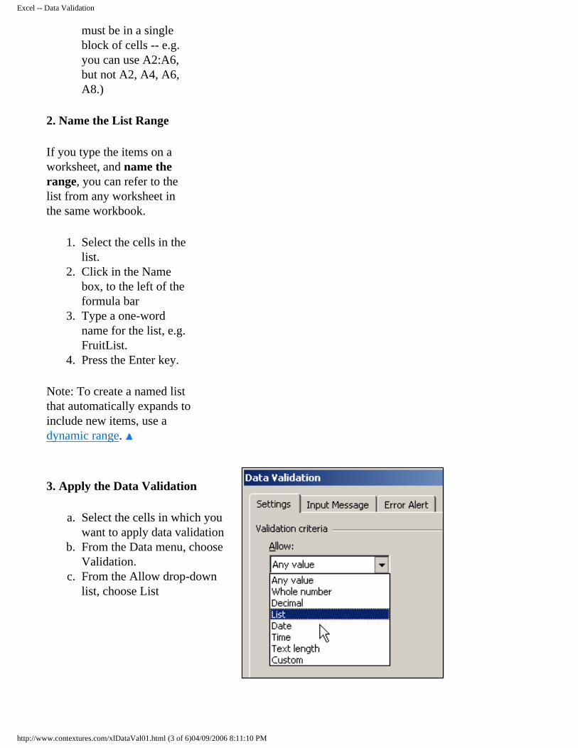
3. Apply the Data Validation
a. Select the cells in which you want to apply data validation
b. From the Data menu, choose Validation.
c. From the Allow drop-down list, choose List
http://www.contextures.com/xlDataVal01.html (3 of 6)04/09/2006 8:11:10 PM
Excel -- Data Validation
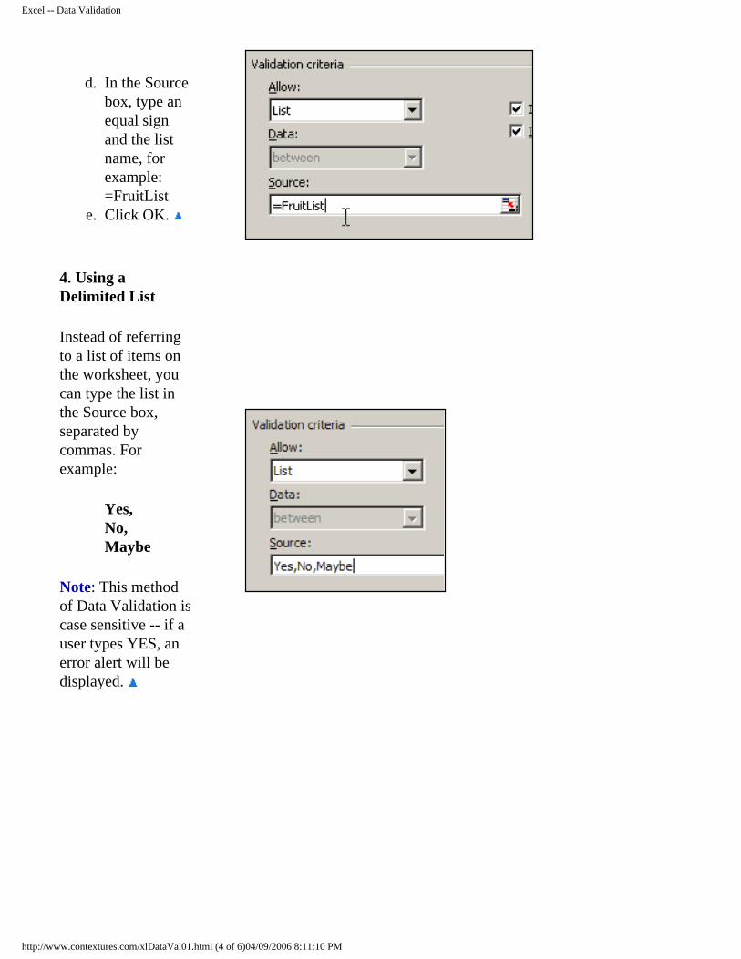
d. In the Source box, type an equal sign and the list name, for example: =FruitList
e. Click OK.
4. Using a Delimited List
Instead of referring to a list of items on the worksheet, you can type the list in the Source box, separated by commas. For example:
Yes,No,Maybe
Note: This method of Data Validation is case sensitive -- if a user types YES, an error alert will be displayed.
http://www.contextures.com/xlDataVal01.html (4 of 6)04/09/2006 8:11:10 PM
Excel -- Data Validation
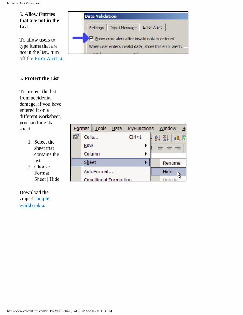
5. Allow Entries that are not in the List
To allow users to type items that are not in the list., turn off the Error Alert.
6. Protect the List
To protect the list from accidental damage, if you have entered it on a different worksheet, you can hide that sheet.
1. Select the sheet that contains the list
2. Choose Format | Sheet | Hide
Download the zipped sample workbook
http://www.contextures.com/xlDataVal01.html (5 of 6)04/09/2006 8:11:10 PM
Excel -- Data Validation
2. Data Validation -- Create Dependent Lists3. Hide Previously Used Items in a Dropdown List4. Display Messages to the User5. Use a List from Another Workbook6. Validation Criteria Examples 7. Custom Validation Criteria Examples 8. Data Validation Tips 9. Data Validation Documentation 10 Data Validation -- Combo box 11. Data Validation -- Combo Box - Named Ranges 12. Data Validation -- Display Input Messages in a Text Box 13. Data Validation -- Dependent Dropdowns from a Sorted List
Home Excel Tips Sample Spreadsheets
Contextures contact information
Last updated: June 4, 2006 11:29 AM
http://www.contextures.com/xlDataVal01.html (6 of 6)04/09/2006 8:11:10 PM
Excel -- Data Validation -- Dependent Lists
Home Excel Tips Sample Spreadsheets
Excel -- Data Validation -- Create Dependent Lists
Create Named Lists Apply the Data Validation Test the Data Validation
Using Two-Word ItemsUsing Items with Illegal CharactersUsing Dynamic Lists
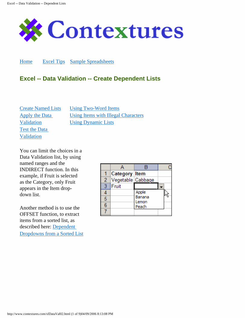
You can limit the choices in a Data Validation list, by using named ranges and the INDIRECT function. In this example, if Fruit is selected as the Category, only Fruit appears in the Item drop-down list.
Another method is to use the OFFSET function, to extract items from a sorted list, as described here: Dependent Dropdowns from a Sorted List
http://www.contextures.com/xlDataVal02.html (1 of 9)04/09/2006 8:13:08 PM
Excel -- Data Validation -- Dependent Lists
Create Named Lists
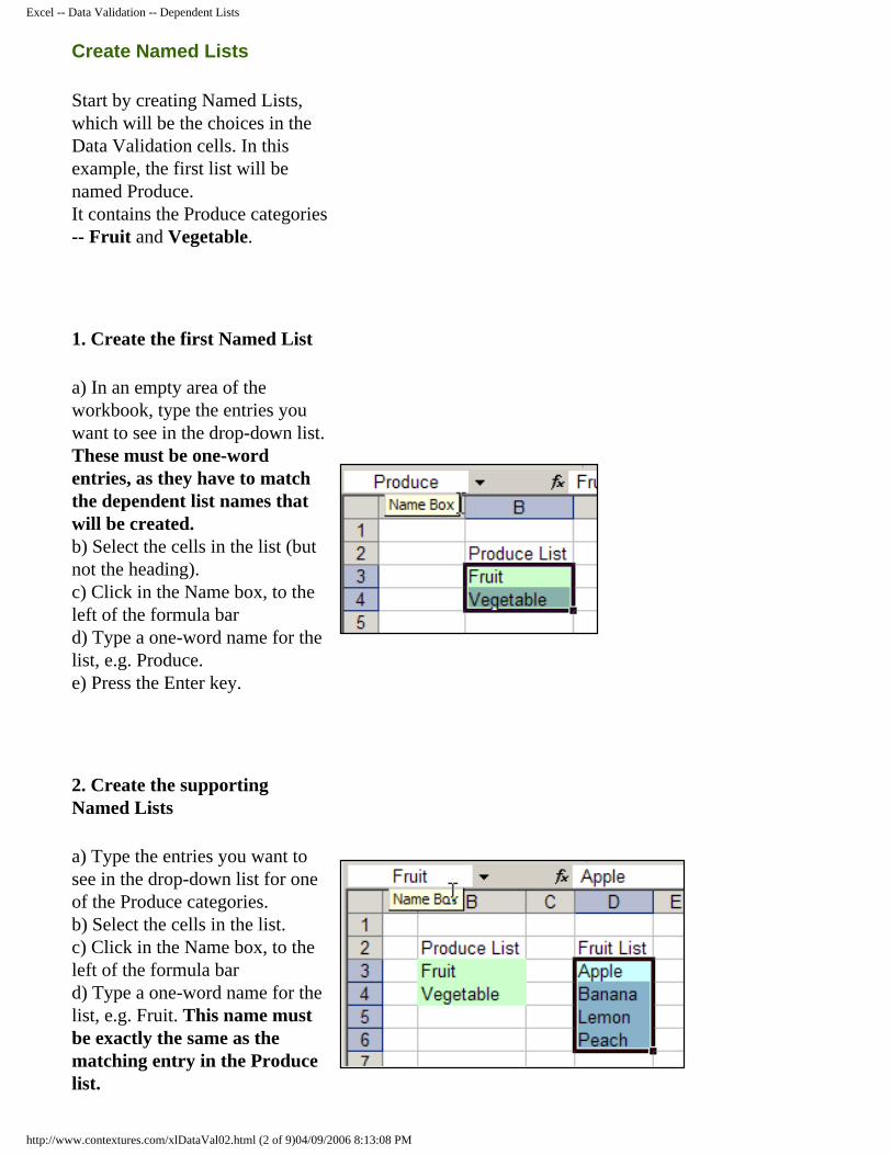
Start by creating Named Lists, which will be the choices in the Data Validation cells. In this example, the first list will be named Produce. It contains the Produce categories -- Fruit and Vegetable.
1. Create the first Named List
a) In an empty area of the workbook, type the entries you want to see in the drop-down list. These must be one-word entries, as they have to match the dependent list names that will be created.b) Select the cells in the list (but not the heading).c) Click in the Name box, to the left of the formula bard) Type a one-word name for the list, e.g. Produce.e) Press the Enter key.
2. Create the supporting Named Lists
a) Type the entries you want to see in the drop-down list for one of the Produce categories.b) Select the cells in the list.c) Click in the Name box, to the left of the formula bard) Type a one-word name for the list, e.g. Fruit. This name must be exactly the same as the matching entry in the Produce list.
http://www.contextures.com/xlDataVal02.html (2 of 9)04/09/2006 8:13:08 PM
Excel -- Data Validation -- Dependent Lists
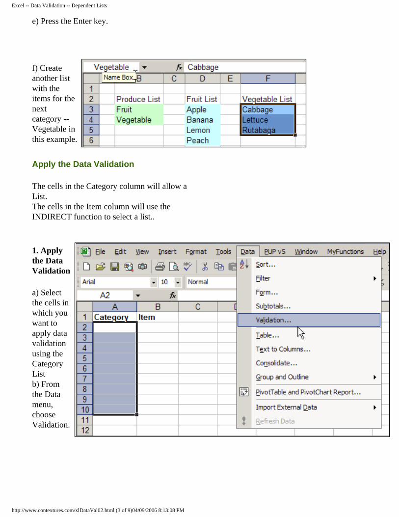
e) Press the Enter key.
f) Create another list with the items for the next category -- Vegetable in this example.
Apply the Data Validation
The cells in the Category column will allow a List. The cells in the Item column will use the INDIRECT function to select a list..
1. Apply the Data Validation
a) Select the cells in which you want to apply data validation using the Category Listb) From the Data menu, choose Validation.
http://www.contextures.com/xlDataVal02.html (3 of 9)04/09/2006 8:13:08 PM
Excel -- Data Validation -- Dependent Lists
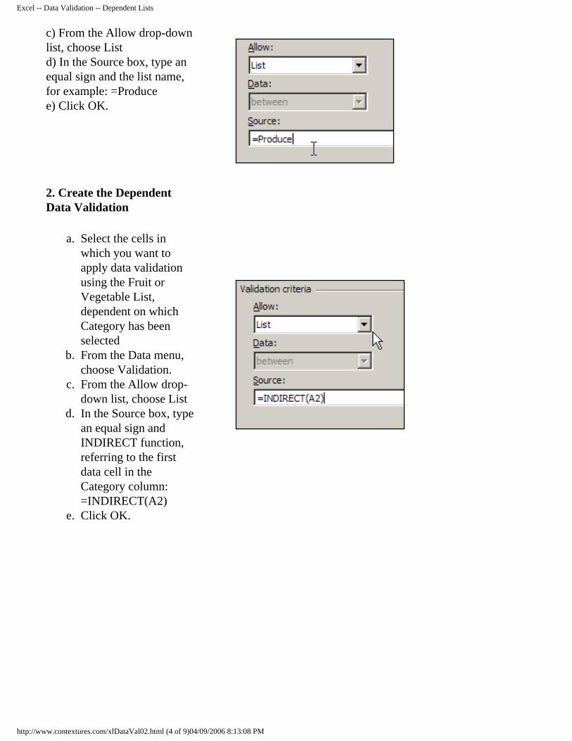
c) From the Allow drop-down list, choose Listd) In the Source box, type an equal sign and the list name, for example: =Produce e) Click OK.
2. Create the Dependent Data Validation
a. Select the cells in which you want to apply data validation using the Fruit or Vegetable List, dependent on which Category has been selected
b. From the Data menu, choose Validation.
c. From the Allow drop-down list, choose List
d. In the Source box, type an equal sign and INDIRECT function, referring to the first data cell in the Category column: =INDIRECT(A2)
e. Click OK.
http://www.contextures.com/xlDataVal02.html (4 of 9)04/09/2006 8:13:08 PM
Excel -- Data Validation -- Dependent Lists
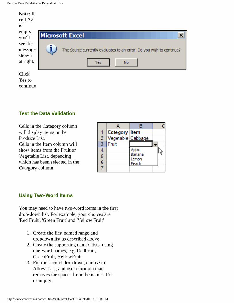
Note: If cell A2 is empty, you'll see the message shown at right.
Click Yes to continue
Test the Data Validation
Cells in the Category column will display items in the Produce List. Cells in the Item column will show items from the Fruit or Vegetable List, depending which has been selected in the Category column
Using Two-Word Items
You may need to have two-word items in the first drop-down list. For example, your choices are 'Red Fruit', 'Green Fruit' and 'Yellow Fruit'
1. Create the first named range and dropdown list as described above.
2. Create the supporting named lists, using one-word names, e.g. RedFruit, GreenFruit, YellowFruit
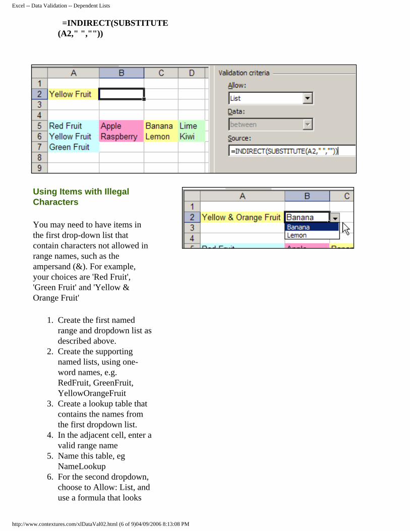
3. For the second dropdown, choose to Allow: List, and use a formula that removes the spaces from the names. For example:
http://www.contextures.com/xlDataVal02.html (5 of 9)04/09/2006 8:13:08 PM
Excel -- Data Validation -- Dependent Lists
=INDIRECT(SUBSTITUTE(A2," ",""))
Using Items with Illegal Characters
You may need to have items in the first drop-down list that contain characters not allowed in range names, such as the ampersand (&). For example, your choices are 'Red Fruit', 'Green Fruit' and 'Yellow & Orange Fruit'
1. Create the first named range and dropdown list as described above.
2. Create the supporting named lists, using one-word names, e.g. RedFruit, GreenFruit, YellowOrangeFruit
3. Create a lookup table that contains the names from the first dropdown list.
4. In the adjacent cell, enter a valid range name
5. Name this table, eg NameLookup
6. For the second dropdown, choose to Allow: List, and use a formula that looks
http://www.contextures.com/xlDataVal02.html (6 of 9)04/09/2006 8:13:08 PM
Excel -- Data Validation -- Dependent Lists
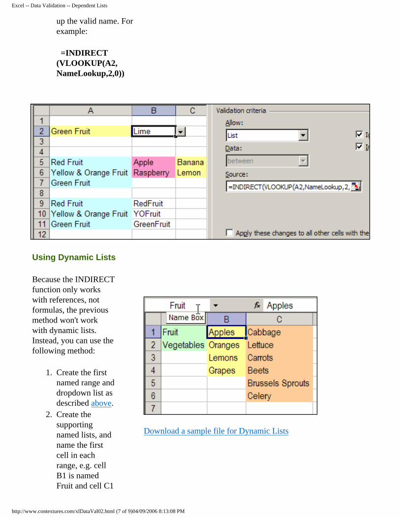
up the valid name. For example:
=INDIRECT(VLOOKUP(A2,NameLookup,2,0))
Using Dynamic Lists
Because the INDIRECT function only works with references, not formulas, the previous method won't work with dynamic lists. Instead, you can use the following method:
1. Create the first named range and dropdown list as described above.
2. Create the supporting named lists, and name the first cell in each range, e.g. cell B1 is named Fruit and cell C1
Download a sample file for Dynamic Lists
http://www.contextures.com/xlDataVal02.html (7 of 9)04/09/2006 8:13:08 PM
Excel -- Data Validation -- Dependent Lists
is named Vegetables.
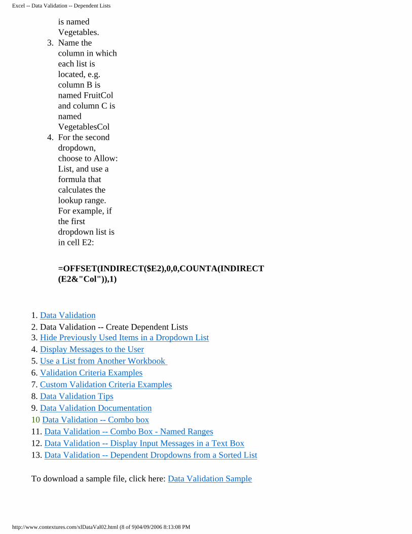
3. Name the column in which each list is located, e.g. column B is named FruitCol and column C is named VegetablesCol
4. For the second dropdown, choose to Allow: List, and use a formula that calculates the lookup range. For example, if the first dropdown list is in cell E2:
=OFFSET(INDIRECT($E2),0,0,COUNTA(INDIRECT(E2&"Col")),1)
1. Data Validation2. Data Validation -- Create Dependent Lists3. Hide Previously Used Items in a Dropdown List4. Display Messages to the User5. Use a List from Another Workbook 6. Validation Criteria Examples 7. Custom Validation Criteria Examples8. Data Validation Tips9. Data Validation Documentation 10 Data Validation -- Combo box 11. Data Validation -- Combo Box - Named Ranges 12. Data Validation -- Display Input Messages in a Text Box 13. Data Validation -- Dependent Dropdowns from a Sorted List
To download a sample file, click here: Data Validation Sample
http://www.contextures.com/xlDataVal02.html (8 of 9)04/09/2006 8:13:08 PM

Excel -- Data Validation -- Dependent Lists
Home Excel Tips Sample Spreadsheets
Contextures contact information
Last updated: June 4, 2006 11:28 AM
http://www.contextures.com/xlDataVal02.html (9 of 9)04/09/2006 8:13:08 PM
Excel -- Data Validation -- Hide Previous Selections
Home Excel Tips Sample Spreadsheets
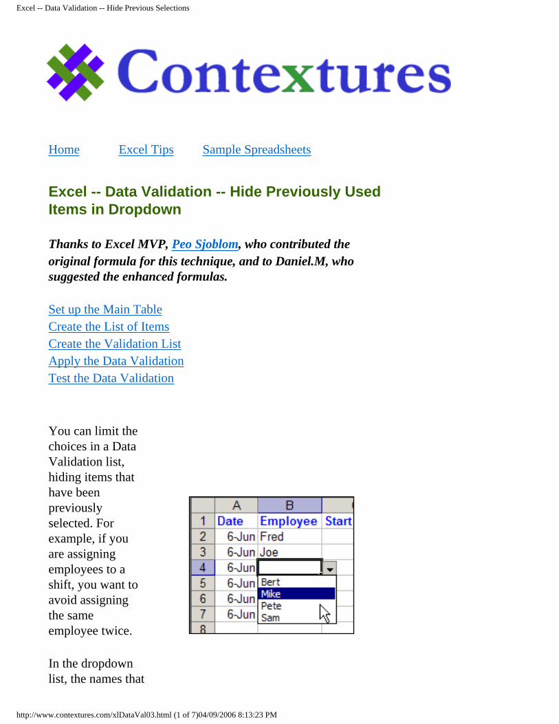
Excel -- Data Validation -- Hide Previously Used Items in Dropdown
Thanks to Excel MVP, Peo Sjoblom, who contributed the original formula for this technique, and to Daniel.M, who suggested the enhanced formulas.
Set up the Main TableCreate the List of ItemsCreate the Validation ListApply the Data ValidationTest the Data Validation
You can limit the choices in a Data Validation list, hiding items that have been previously selected. For example, if you are assigning employees to a shift, you want to avoid assigning the same employee twice.
In the dropdown list, the names that
http://www.contextures.com/xlDataVal03.html (1 of 7)04/09/2006 8:13:23 PM
Excel -- Data Validation -- Hide Previous Selections
have been used are removed.
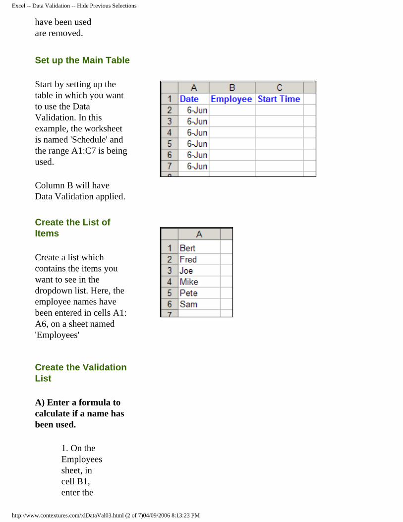
Set up the Main Table
Start by setting up the table in which you want to use the Data Validation. In this example, the worksheet is named 'Schedule' and the range A1:C7 is being used.
Column B will have Data Validation applied.
Create the List of Items
Create a list which contains the items you want to see in the dropdown list. Here, the employee names have been entered in cells A1:A6, on a sheet named 'Employees'
Create the Validation List
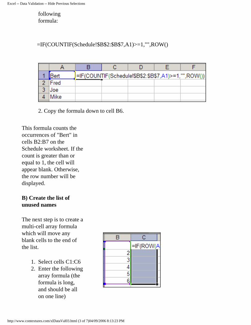
A) Enter a formula to calculate if a name has been used.
1. On the Employees sheet, in cell B1, enter the
http://www.contextures.com/xlDataVal03.html (2 of 7)04/09/2006 8:13:23 PM
Excel -- Data Validation -- Hide Previous Selections
following formula:
=IF(COUNTIF(Schedule!$B$2:$B$7,A1)>=1,"",ROW()
2. Copy the formula down to cell B6.
This formula counts the occurrences of "Bert" in cells B2:B7 on the Schedule worksheet. If the count is greater than or equal to 1, the cell will appear blank. Otherwise, the row number will be displayed.
B) Create the list of unused names
The next step is to create a multi-cell array formula which will move any blank cells to the end of the list.
1. Select cells C1:C6 2. Enter the following
array formula (the formula is long, and should be all on one line)
http://www.contextures.com/xlDataVal03.html (3 of 7)04/09/2006 8:13:23 PM
Excel -- Data Validation -- Hide Previous Selections
=IF(ROW(A1:A6)-ROW(A1)+1>COUNT(B1:B6),"", INDEX(A:A,SMALL(B1:B6,ROW(INDIRECT("1:"&ROWS(A1:A6))))))
3. Press Ctrl+Shift+Enter to enter the array formula in cells C1:C6
Single-Cell Formula Alternative
If you'd prefer a single-cell formula (easier to edit), you could use this formula, also by Daniel.M. He recommends it for small ranges (<=200 cells):
1. Select cell C12. Enter the following formula (the
formula is long, and should be all on one line)
=IF(ROW(A1)-ROW(A$1)+1>COUNT(B$1:B$6),"",INDEX(A:A,SMALL(B$1:B$6,1+ROW(A1)-ROW(A$1))))
3. Press Enter 4. Copy the formula down to row 6
http://www.contextures.com/xlDataVal03.html (4 of 7)04/09/2006 8:13:23 PM
Excel -- Data Validation -- Hide Previous Selections
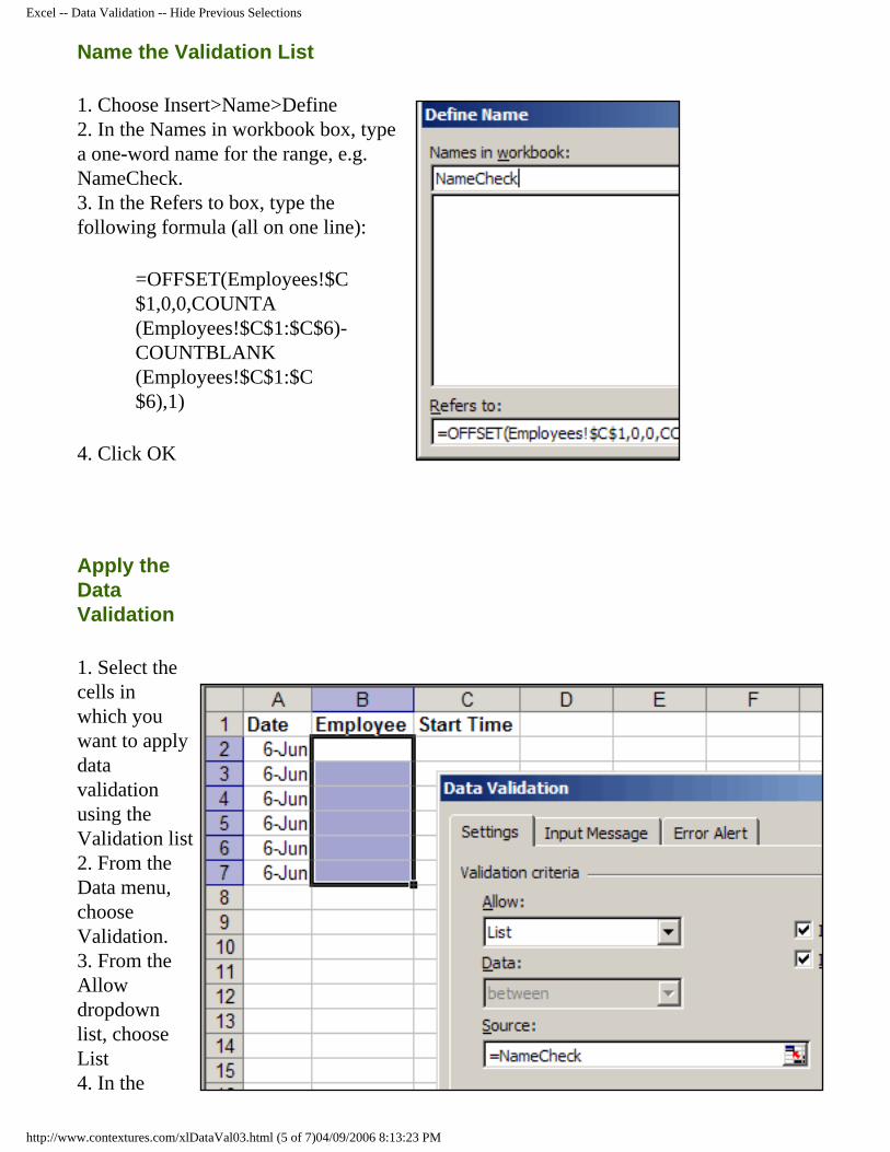
Name the Validation List
1. Choose Insert>Name>Define2. In the Names in workbook box, type a one-word name for the range, e.g. NameCheck.3. In the Refers to box, type the following formula (all on one line):
=OFFSET(Employees!$C$1,0,0,COUNTA(Employees!$C$1:$C$6)-COUNTBLANK(Employees!$C$1:$C$6),1)
4. Click OK
Apply the Data Validation
1. Select the cells in which you want to apply data validation using the Validation list2. From the Data menu, choose Validation.3. From the Allow dropdown list, choose List4. In the
http://www.contextures.com/xlDataVal03.html (5 of 7)04/09/2006 8:13:23 PM
Excel -- Data Validation -- Hide Previous Selections
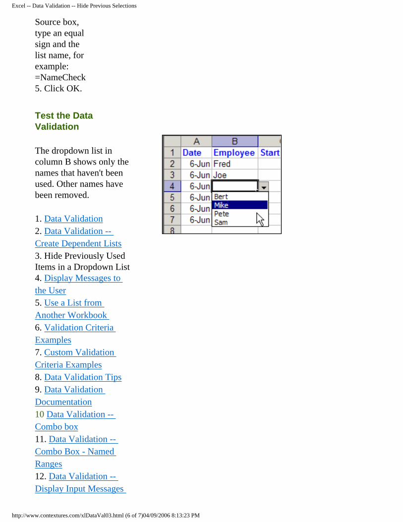
Source box, type an equal sign and the list name, for example: =NameCheck 5. Click OK.
Test the Data Validation
The dropdown list in column B shows only the names that haven't been used. Other names have been removed.
1. Data Validation2. Data Validation -- Create Dependent Lists3. Hide Previously Used Items in a Dropdown List4. Display Messages to the User5. Use a List from Another Workbook 6. Validation Criteria Examples 7. Custom Validation Criteria Examples8. Data Validation Tips 9. Data Validation Documentation 10 Data Validation -- Combo box 11. Data Validation -- Combo Box - Named Ranges 12. Data Validation -- Display Input Messages
http://www.contextures.com/xlDataVal03.html (6 of 7)04/09/2006 8:13:23 PM
Excel -- Data Validation -- Hide Previous Selections
in a Text Box 13. Data Validation -- Dependent Dropdowns from a Sorted List
To download a zipped sample file, click here: Data Validation -- Hidden Items -- Sample
Home Excel Tips Sample Spreadsheets
Contextures contact information
Last updated: June 4, 2006 10:27 AM
http://www.contextures.com/xlDataVal03.html (7 of 7)04/09/2006 8:13:23 PM
Excel -- Data Validation -- Add Message for User
Home Excel Tips Sample Spreadsheets
Excel -- Data Validation -- Add Messages to Help the User
Input MessageError Alert
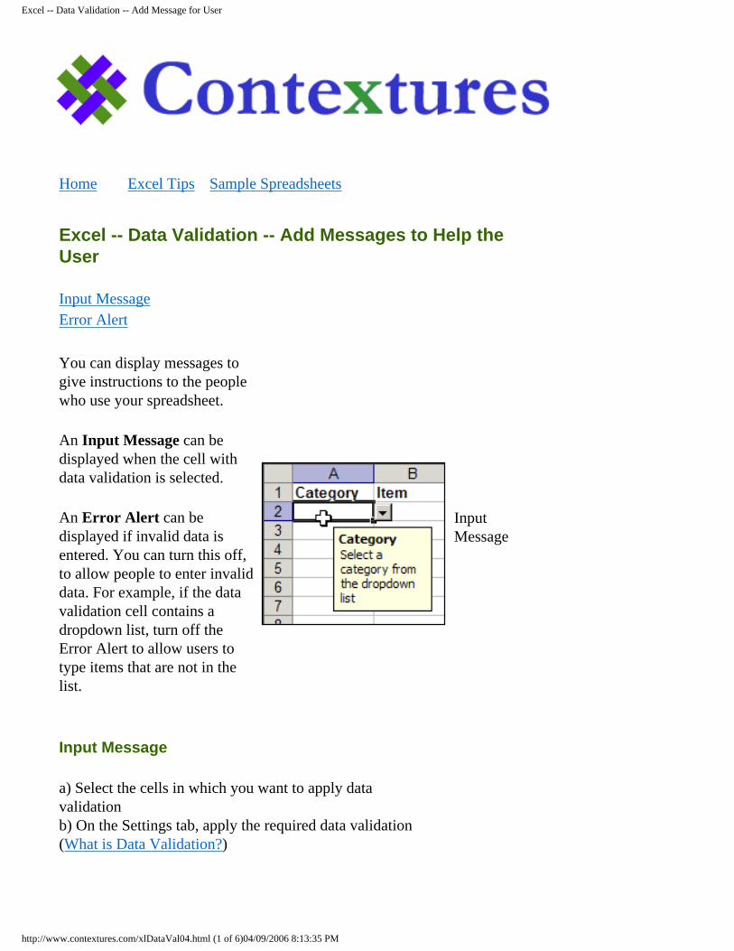
You can display messages to give instructions to the people who use your spreadsheet.
An Input Message can be displayed when the cell with data validation is selected.
An Error Alert can be displayed if invalid data is entered. You can turn this off, to allow people to enter invalid data. For example, if the data validation cell contains a dropdown list, turn off the Error Alert to allow users to type items that are not in the list.
Input Message
Input Message
a) Select the cells in which you want to apply data validationb) On the Settings tab, apply the required data validation (What is Data Validation?)
http://www.contextures.com/xlDataVal04.html (1 of 6)04/09/2006 8:13:35 PM
Excel -- Data Validation -- Add Message for User
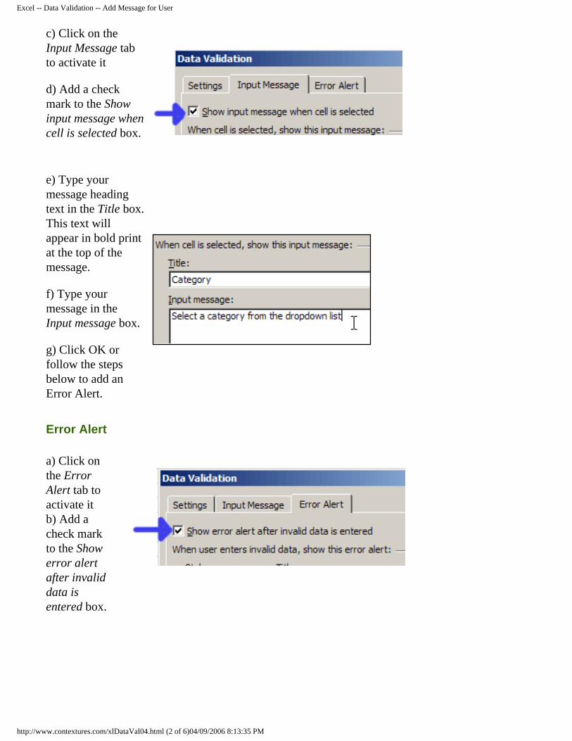
c) Click on the Input Message tab to activate it
d) Add a check mark to the Show input message when cell is selected box.
e) Type your message heading text in the Title box. This text will appear in bold print at the top of the message.
f) Type your message in the Input message box.
g) Click OK or follow the steps below to add an Error Alert.
Error Alert
a) Click on the Error Alert tab to activate it b) Add a check mark to the Show error alert after invalid data is entered box.
http://www.contextures.com/xlDataVal04.html (2 of 6)04/09/2006 8:13:35 PM
Excel -- Data Validation -- Add Message for User
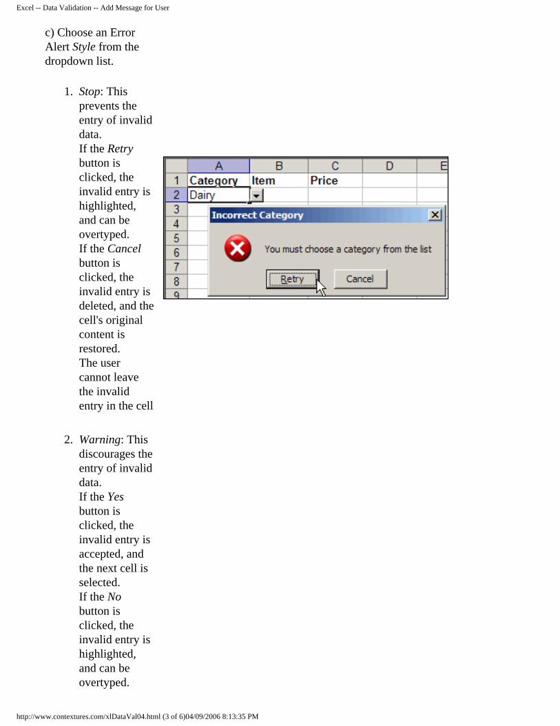
c) Choose an Error Alert Style from the dropdown list.
1. Stop: This prevents the entry of invalid data. If the Retry button is clicked, the invalid entry is highlighted, and can be overtyped. If the Cancel button is clicked, the invalid entry is deleted, and the cell's original content is restored.The user cannot leave the invalid entry in the cell
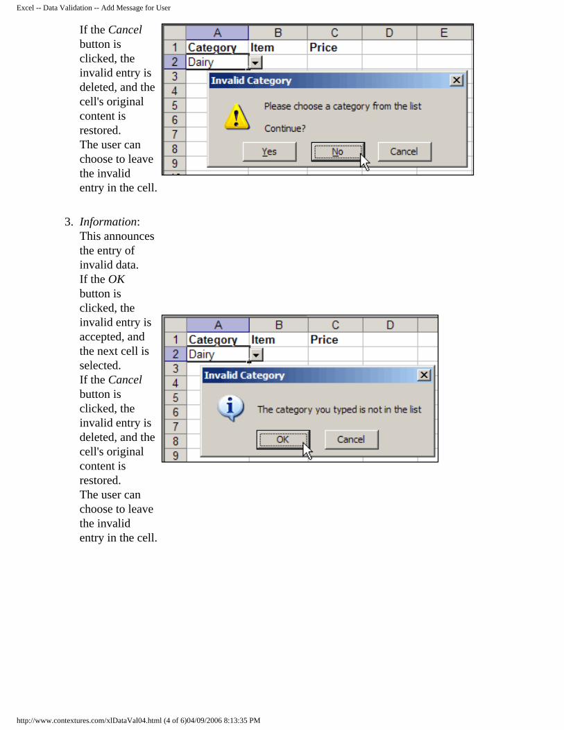
2. Warning: This discourages the entry of invalid data. If the Yes button is clicked, the invalid entry is accepted, and the next cell is selected. If the No button is clicked, the invalid entry is highlighted, and can be overtyped.
http://www.contextures.com/xlDataVal04.html (3 of 6)04/09/2006 8:13:35 PM
Excel -- Data Validation -- Add Message for User
If the Cancel button is clicked, the invalid entry is deleted, and the cell's original content is restored.The user can choose to leave the invalid entry in the cell.
3. Information: This announces the entry of invalid data. If the OK button is clicked, the invalid entry is accepted, and the next cell is selected. If the Cancel button is clicked, the invalid entry is deleted, and the cell's original content is restored.The user can choose to leave the invalid entry in the cell.
http://www.contextures.com/xlDataVal04.html (4 of 6)04/09/2006 8:13:35 PM
Excel -- Data Validation -- Add Message for User
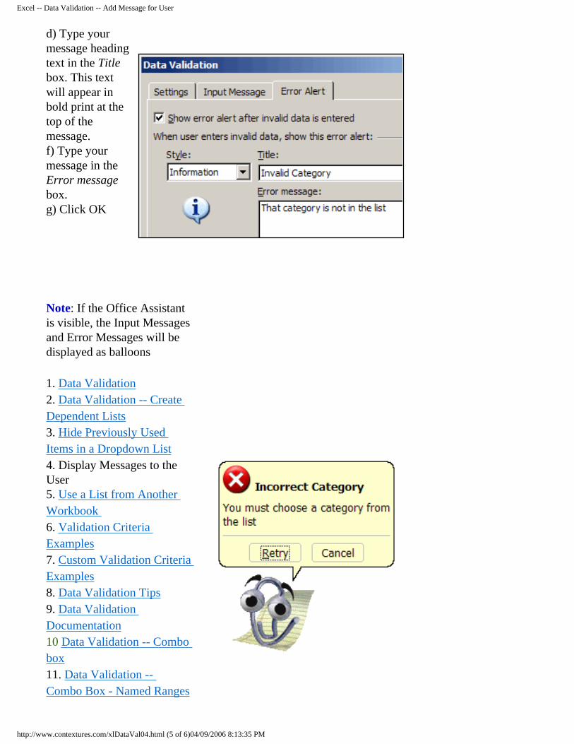
d) Type your message heading text in the Title box. This text will appear in bold print at the top of the message.f) Type your message in the Error message box.g) Click OK
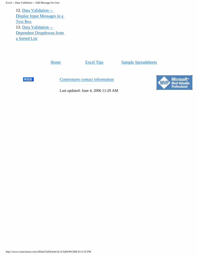
Note: If the Office Assistant is visible, the Input Messages and Error Messages will be displayed as balloons
1. Data Validation2. Data Validation -- Create Dependent Lists3. Hide Previously Used Items in a Dropdown List4. Display Messages to the User5. Use a List from Another Workbook 6. Validation Criteria Examples 7. Custom Validation Criteria Examples8. Data Validation Tips 9. Data Validation Documentation 10 Data Validation -- Combo box 11. Data Validation -- Combo Box - Named Ranges
http://www.contextures.com/xlDataVal04.html (5 of 6)04/09/2006 8:13:35 PM
Excel -- Data Validation -- Add Message for User
12. Data Validation -- Display Input Messages in a Text Box 13. Data Validation -- Dependent Dropdowns from a Sorted List
Home Excel Tips Sample Spreadsheets
Contextures contact information
Last updated: June 4, 2006 11:29 AM
http://www.contextures.com/xlDataVal04.html (6 of 6)04/09/2006 8:13:35 PM
Excel -- Data Validation -- Use List from Another Workbook
Home Excel Tips Sample Spreadsheets
Excel -- Data Validation -- Use a List from Another Workbook
Create the Source ListCreate a Reference to the Source ListCreate the Dropdown ListCreate a Dynamic Range from Another Workbook
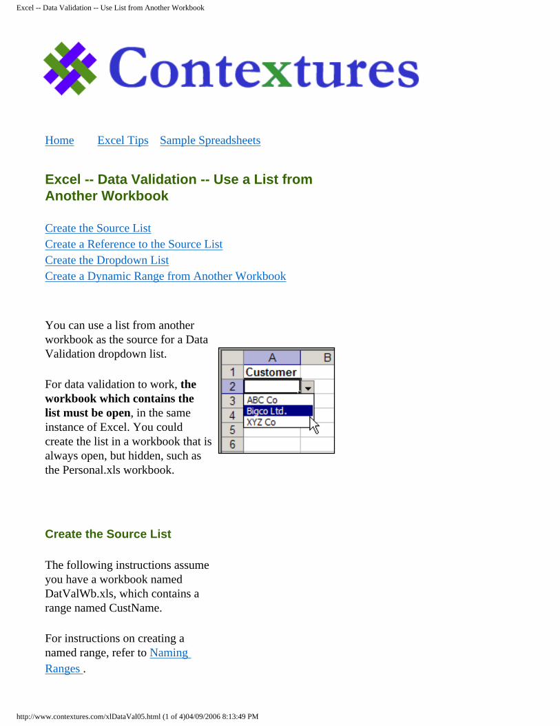
You can use a list from another workbook as the source for a Data Validation dropdown list.
For data validation to work, the workbook which contains the list must be open, in the same instance of Excel. You could create the list in a workbook that is always open, but hidden, such as the Personal.xls workbook.
Create the Source List
The following instructions assume you have a workbook named DatValWb.xls, which contains a range named CustName.
For instructions on creating a named range, refer to Naming Ranges .
http://www.contextures.com/xlDataVal05.html (1 of 4)04/09/2006 8:13:49 PM
Excel -- Data Validation -- Use List from Another Workbook
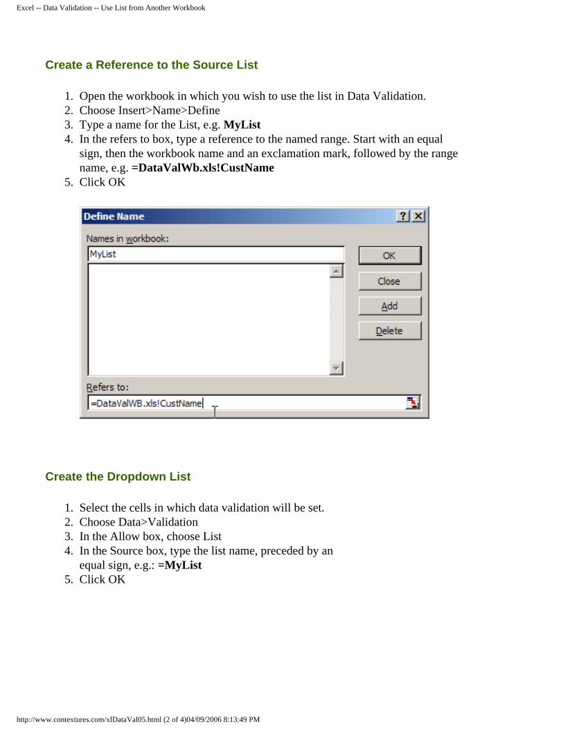
Create a Reference to the Source List
1. Open the workbook in which you wish to use the list in Data Validation.2. Choose Insert>Name>Define3. Type a name for the List, e.g. MyList4. In the refers to box, type a reference to the named range. Start with an equal
sign, then the workbook name and an exclamation mark, followed by the range name, e.g. =DataValWb.xls!CustName
5. Click OK
Create the Dropdown List
1. Select the cells in which data validation will be set. 2. Choose Data>Validation 3. In the Allow box, choose List 4. In the Source box, type the list name, preceded by an
equal sign, e.g.: =MyList 5. Click OK
http://www.contextures.com/xlDataVal05.html (2 of 4)04/09/2006 8:13:49 PM
Excel -- Data Validation -- Use List from Another Workbook
Create a Dynamic Range from Another Workbook
You can create a dynamic range that refers to a dynamic range in another (open) workbook.
1. Create and save a workbook (MyLists.xls, in this example)
2. Enter a list of names in cells A1:A10 on Sheet 1.3. To create a dynamic range, choose Insert|Name|
DefineUse Employees as the range name, and the following formula: =OFFSET(Sheet1!$A$1,0,0,COUNTA(Sheet1!$A:$A))
4. Keep MyLists.xls open, and create and save a new workbook (Schedule.xls)
5. In Schedule.xls, create a range named EmployeeList with this formula: =MyLists.xls!Employees
6. In cell A1 of sheet1, enter the following formula: =EmployeeList
7. Copy the formula down to row 200 (or any row beyond the length of the dynamic range in MyList.xls). Note: many of the rows will contain a #VALUE! error.
8. In Schedule.xls, create another range, with the name NoErrors, and the formula:
=OFFSET(Sheet1!$A$1,0,0,COUNTA(Sheet1!$A:$A)-COUNTIF(Sheet1!$A$1:$A$300,"#VALUE! ")) (all one line)
8. Use NoErrors as the source for your Data Validation list.
http://www.contextures.com/xlDataVal05.html (3 of 4)04/09/2006 8:13:49 PM
Excel -- Data Validation -- Use List from Another Workbook
1. Data Validation2. Data Validation -- Create Dependent Lists3. Hide Previously Used Items in a Dropdown List4. Display Messages to the User5. Use a List from Another Workbook 6. Validation Criteria Examples 7. Custom Validation Criteria Examples8. Data Validation Tips9. Data Validation Documentation 10 Data Validation -- Combo box 11. Data Validation -- Combo Box - Named Ranges 12. Data Validation -- Display Input Messages in a Text Box 13. Data Validation -- Dependent Dropdowns from a Sorted List
Home Excel Tips Sample Spreadsheets
Contextures contact information
Last updated: June 4, 2006 11:09 AM
http://www.contextures.com/xlDataVal05.html (4 of 4)04/09/2006 8:13:49 PM
Excel -- Data Validation -- Validation Criteria Examples
Home Excel Tips Sample Spreadsheets
Excel -- Data Validation -- Validation Criteria Examples
Whole NumberDecimal
ListDate
TimeText Length
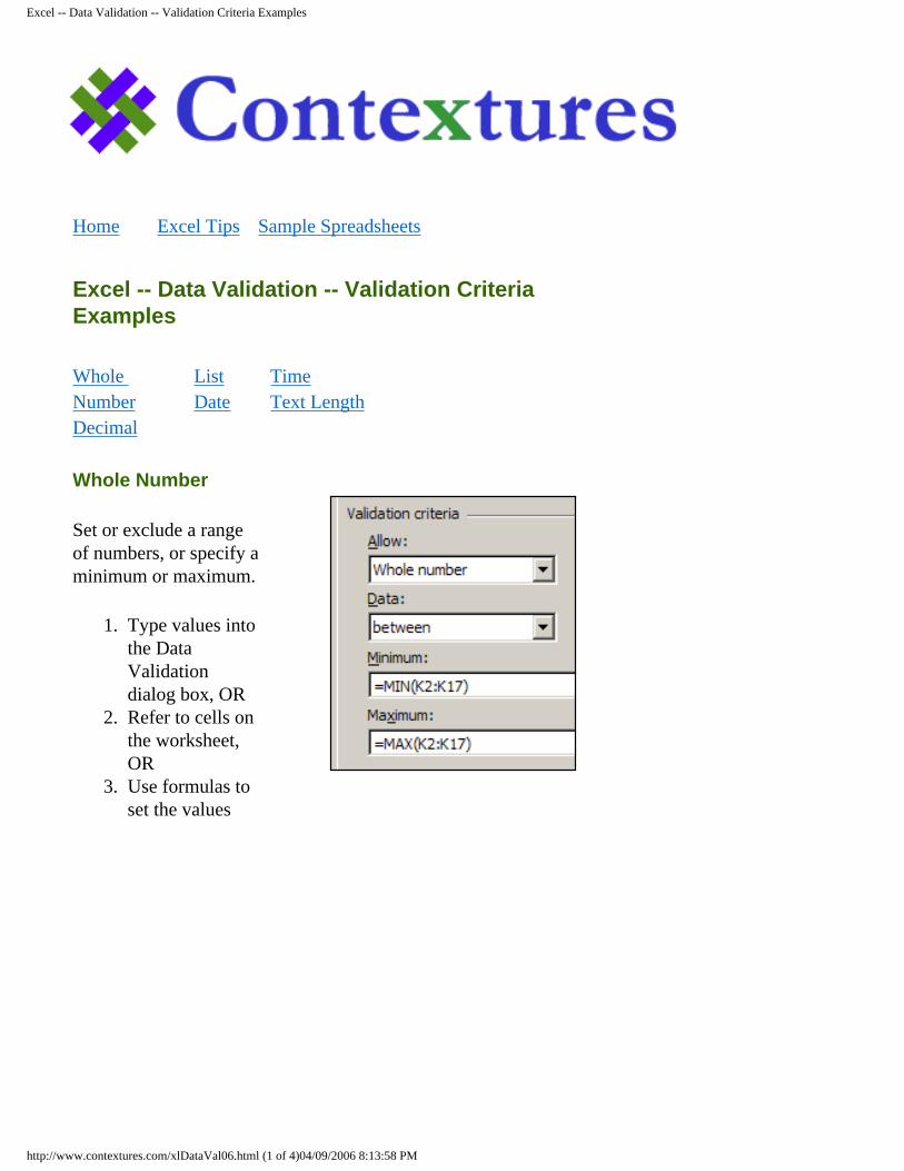
Whole Number
Set or exclude a range of numbers, or specify a minimum or maximum.
1. Type values into the Data Validation dialog box, OR
2. Refer to cells on the worksheet, OR
3. Use formulas to set the values
http://www.contextures.com/xlDataVal06.html (1 of 4)04/09/2006 8:13:58 PM
Excel -- Data Validation -- Validation Criteria Examples
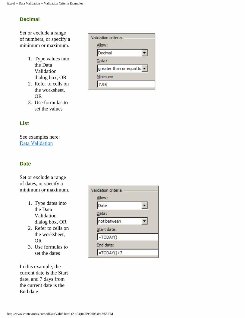
Decimal
Set or exclude a range of numbers, or specify a minimum or maximum.
1. Type values into the Data Validation dialog box, OR
2. Refer to cells on the worksheet, OR
3. Use formulas to set the values
List
See examples here: Data Validation
Date
Set or exclude a range of dates, or specify a minimum or maximum.
1. Type dates into the Data Validation dialog box, OR
2. Refer to cells on the worksheet, OR
3. Use formulas to set the dates
In this example, the current date is the Start date, and 7 days from the current date is the End date:
http://www.contextures.com/xlDataVal06.html (2 of 4)04/09/2006 8:13:58 PM
Excel -- Data Validation -- Validation Criteria Examples
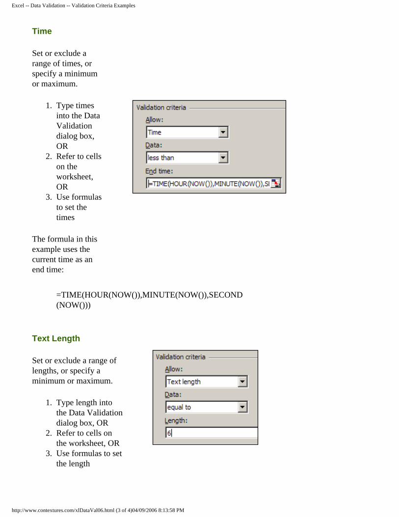
Time
Set or exclude a range of times, or specify a minimum or maximum.
1. Type times into the Data Validation dialog box, OR
2. Refer to cells on the worksheet, OR
3. Use formulas to set the times
The formula in this example uses the current time as an end time:
=TIME(HOUR(NOW()),MINUTE(NOW()),SECOND(NOW()))
Text Length
Set or exclude a range of lengths, or specify a minimum or maximum.
1. Type length into the Data Validation dialog box, OR
2. Refer to cells on the worksheet, OR
3. Use formulas to set the length
http://www.contextures.com/xlDataVal06.html (3 of 4)04/09/2006 8:13:58 PM
Excel -- Data Validation -- Validation Criteria Examples
1. Data Validation2. Data Validation -- Create Dependent Lists3. Hide Previously Used Items in a Dropdown List4. Display Messages to the User5. Use a List from Another Workbook 6. Validation Criteria Examples 7. Custom Validation Criteria Examples8. Data Validation Tips9. Data Validation Documentation 10 Data Validation -- Combo box 11. Data Validation -- Combo Box - Named Ranges 12. Data Validation -- Display Input Messages in a Text Box 13. Data Validation -- Dependent Dropdowns from a Sorted List
Home Excel Tips Sample Spreadsheets
Contextures contact information
Last updated: June 4, 2006 11:29 AM
http://www.contextures.com/xlDataVal06.html (4 of 4)04/09/2006 8:13:58 PM
Excel -- Data Validation -- Custom Validation Criteria Examples
Home Excel Tips Sample Spreadsheets
Excel -- Data Validation -- Custom Validation Criteria Examples
Prevent DuplicatesLimit the Total
No Leading or Trailing SpacesProhibit Weekend Dates
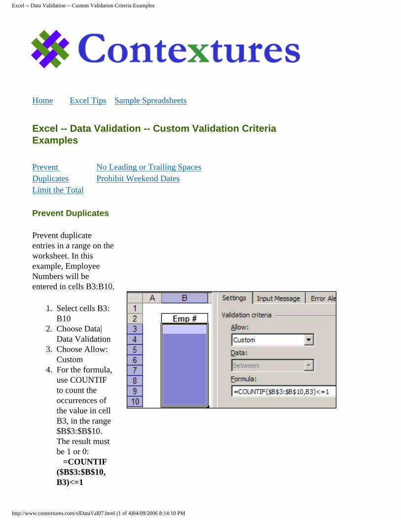
Prevent Duplicates
Prevent duplicate entries in a range on the worksheet. In this example, Employee Numbers will be entered in cells B3:B10.
1. Select cells B3:B10
2. Choose Data|Data Validation
3. Choose Allow: Custom
4. For the formula, use COUNTIF to count the occurrences of the value in cell B3, in the range $B$3:$B$10. The result must be 1 or 0: =COUNTIF($B$3:$B$10,B3)<=1
http://www.contextures.com/xlDataVal07.html (1 of 4)04/09/2006 8:14:10 PM
Excel -- Data Validation -- Custom Validation Criteria Examples
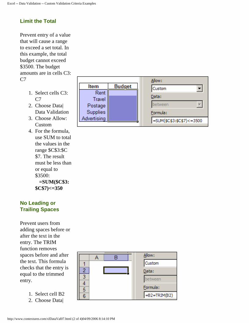
Limit the Total
Prevent entry of a value that will cause a range to exceed a set total. In this example, the total budget cannot exceed $3500. The budget amounts are in cells C3:C7
1. Select cells C3:C7
2. Choose Data|Data Validation
3. Choose Allow: Custom
4. For the formula, use SUM to total the values in the range $C$3:$C$7. The result must be less than or equal to $3500: =SUM($C$3:$C$7)<=350
No Leading or Trailing Spaces
Prevent users from adding spaces before or after the text in the entry. The TRIM function removes spaces before and after the text. This formula checks that the entry is equal to the trimmed entry.
1. Select cell B22. Choose Data|
http://www.contextures.com/xlDataVal07.html (2 of 4)04/09/2006 8:14:10 PM
Excel -- Data Validation -- Custom Validation Criteria Examples
Data Validation3. Choose Allow:
Custom4. For the formula,
enter: =B2=TRIM(B2)
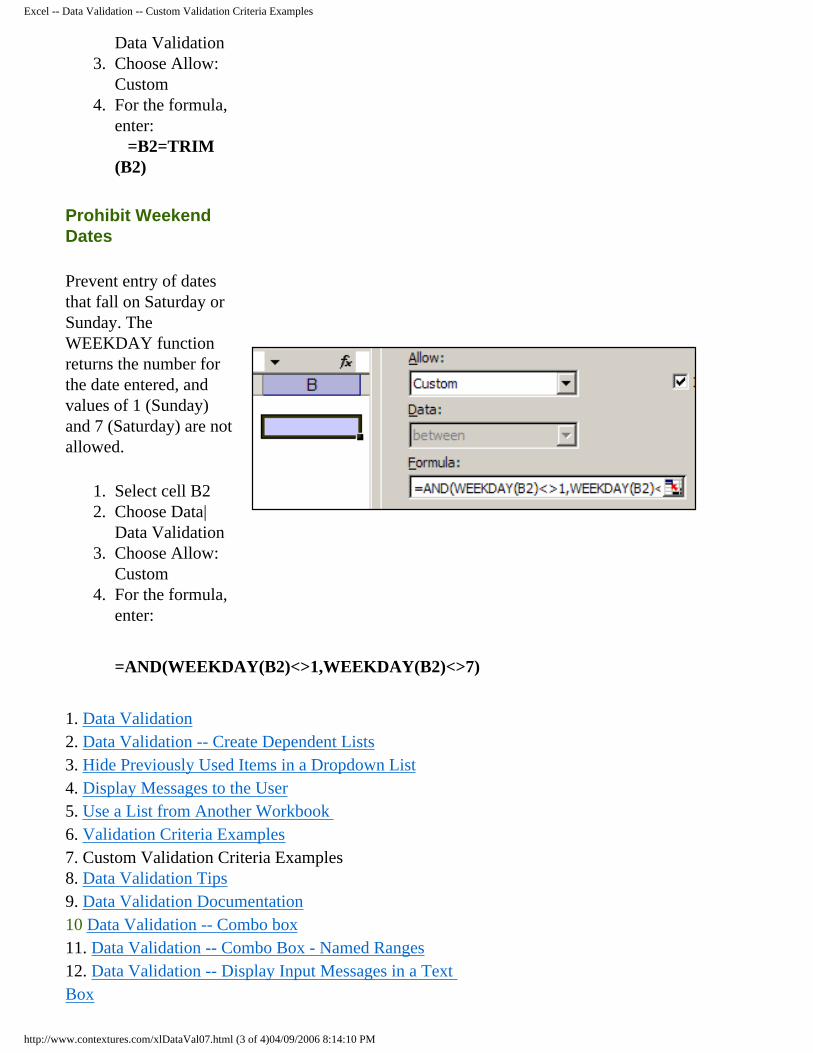
Prohibit Weekend Dates
Prevent entry of dates that fall on Saturday or Sunday. The WEEKDAY function returns the number for the date entered, and values of 1 (Sunday) and 7 (Saturday) are not allowed.
1. Select cell B22. Choose Data|
Data Validation3. Choose Allow:
Custom4. For the formula,
enter:
=AND(WEEKDAY(B2)<>1,WEEKDAY(B2)<>7)
1. Data Validation2. Data Validation -- Create Dependent Lists3. Hide Previously Used Items in a Dropdown List4. Display Messages to the User5. Use a List from Another Workbook 6. Validation Criteria Examples 7. Custom Validation Criteria Examples8. Data Validation Tips9. Data Validation Documentation 10 Data Validation -- Combo box 11. Data Validation -- Combo Box - Named Ranges 12. Data Validation -- Display Input Messages in a Text Box
http://www.contextures.com/xlDataVal07.html (3 of 4)04/09/2006 8:14:10 PM

Excel -- Data Validation -- Custom Validation Criteria Examples
13. Data Validation -- Dependent Dropdowns from a Sorted List
Home Excel Tips Sample Spreadsheets
Contextures contact information
Last updated: June 4, 2006 11:30 AM
http://www.contextures.com/xlDataVal07.html (4 of 4)04/09/2006 8:14:10 PM
Excel -- Data Validation -- AdvancedTechniques
Home Excel Tips Sample Spreadsheets
Excel -- Data Validation -- Tips
Use Dynamic ListsData Validation Font Size and List LengthData Validation Dropdowns and Change Events Data Validation Dropdowns and Freeze Panes Data Validation on a Protected Sheet Make the Dropdown List Temporarily WiderMake the Dropdown List Appear Larger -- Zoom in when specific cell is selected -- Zoom in when specific cells are selected -- Zoom in when any cell with data validation is selected
Use Dynamic Lists
Some lists change frequently, with items being added or removed. If the list is the source for a Data Validation dropdown, use a dynamic formula to name the range, and the dropdown list will be automatically updated.
For instructions, view this page: Create a Dynamic Range
Data Validation Dropdowns and Change Events
In Excel 2000 and later versions, selecting an item from a Data Validation dropdown list will trigger a Change event. This means that code can automatically run after a user selects an item from the list.
To see an example, go to the Sample Worksheets page, and under the Filters heading, find Product List by Category, and download the ProductsList.zip file.
In Excel 97, selecting an item from a Data Validation dropdown list does not trigger a Change event, unless the list items have been typed in the Data Validation dialog box. In this version, you can add a button to the worksheet, and run the code by clicking the button. To see an example, go to the Sample Worksheets page, and under the Filters heading, find Product List by Category, and download the ProductsList97.zip file.
Another option in Excel 97 is to use the Calculate event to run the
http://www.contextures.com/xlDataVal08.html (1 of 5)04/09/2006 8:14:25 PM
Excel -- Data Validation -- AdvancedTechniques
code. To do this, refer to the cell with data validation in a formula on the worksheet, e.g. =MATCH(C3,CategoryList,0). Then, add the filter code to the worksheet's Calculate event. To see an example, go to the Sample Worksheets page, and under the Filters heading, find Product List by Category, and download the ProductsList97Calc.zip file.
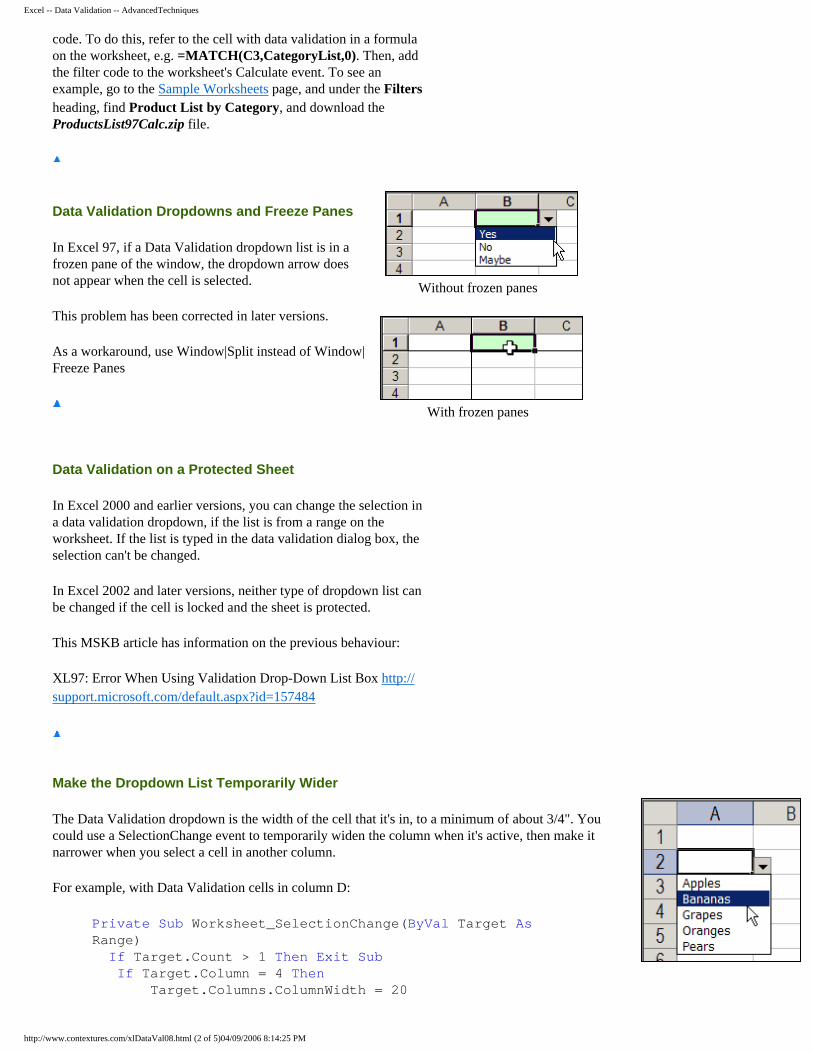
Data Validation Dropdowns and Freeze Panes
In Excel 97, if a Data Validation dropdown list is in a frozen pane of the window, the dropdown arrow does not appear when the cell is selected.
This problem has been corrected in later versions.
As a workaround, use Window|Split instead of Window|Freeze Panes
Without frozen panes
With frozen panes
Data Validation on a Protected Sheet
In Excel 2000 and earlier versions, you can change the selection in a data validation dropdown, if the list is from a range on the worksheet. If the list is typed in the data validation dialog box, the selection can't be changed.
In Excel 2002 and later versions, neither type of dropdown list can be changed if the cell is locked and the sheet is protected.
This MSKB article has information on the previous behaviour:
XL97: Error When Using Validation Drop-Down List Box http://support.microsoft.com/default.aspx?id=157484
Make the Dropdown List Temporarily Wider
The Data Validation dropdown is the width of the cell that it's in, to a minimum of about 3/4". You could use a SelectionChange event to temporarily widen the column when it's active, then make it narrower when you select a cell in another column.
For example, with Data Validation cells in column D:
Private Sub Worksheet_SelectionChange(ByVal Target As Range) If Target.Count > 1 Then Exit Sub If Target.Column = 4 Then Target.Columns.ColumnWidth = 20
http://www.contextures.com/xlDataVal08.html (2 of 5)04/09/2006 8:14:25 PM
Excel -- Data Validation -- AdvancedTechniques
Else Columns(4).ColumnWidth = 5 End If End Sub
To add this code to the worksheet:
1. Right-click on the sheet tab, and choose View Code. 2. Copy the code, and paste it onto the code module. 3. Change the column reference from 4 to match your worksheet.
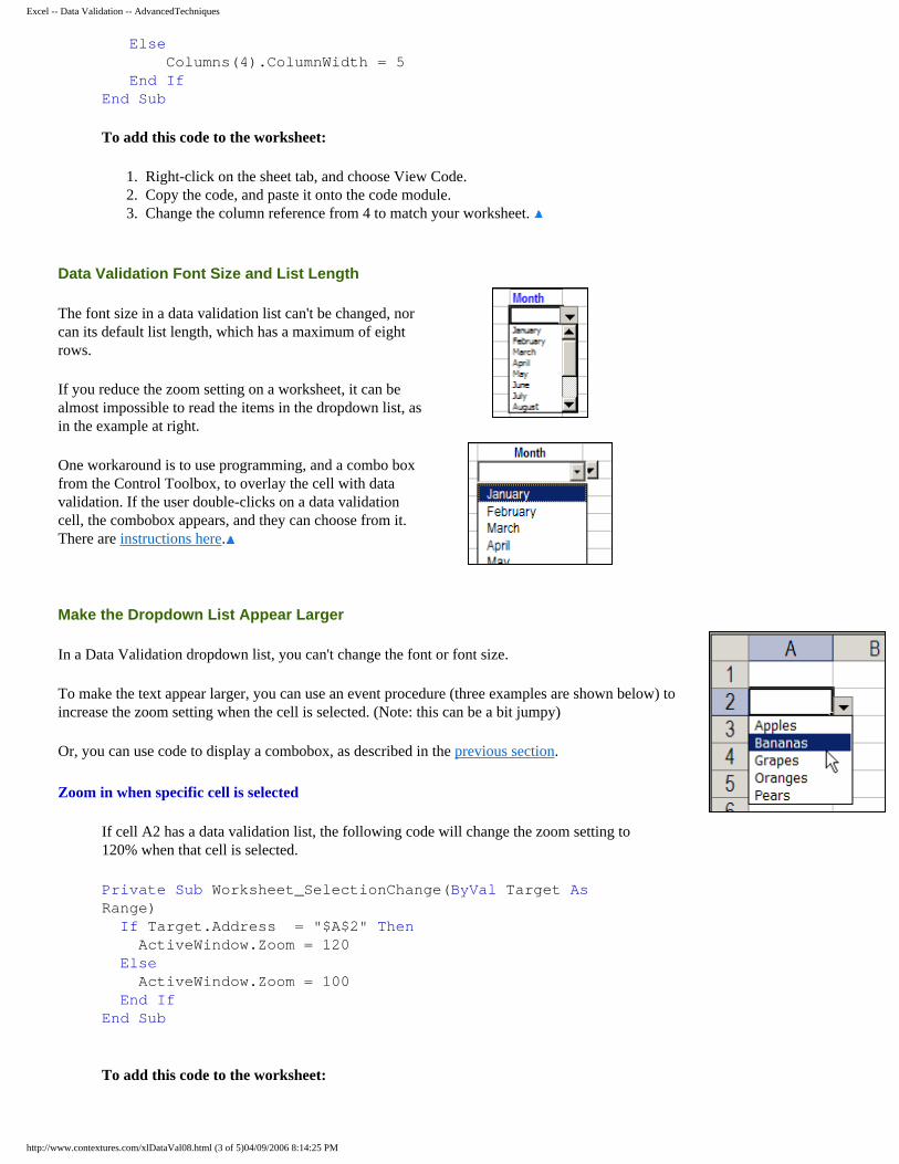
Data Validation Font Size and List Length
The font size in a data validation list can't be changed, nor can its default list length, which has a maximum of eight rows.
If you reduce the zoom setting on a worksheet, it can be almost impossible to read the items in the dropdown list, as in the example at right.
One workaround is to use programming, and a combo box from the Control Toolbox, to overlay the cell with data validation. If the user double-clicks on a data validation cell, the combobox appears, and they can choose from it. There are instructions here.
Make the Dropdown List Appear Larger
In a Data Validation dropdown list, you can't change the font or font size.
To make the text appear larger, you can use an event procedure (three examples are shown below) to increase the zoom setting when the cell is selected. (Note: this can be a bit jumpy)
Or, you can use code to display a combobox, as described in the previous section.
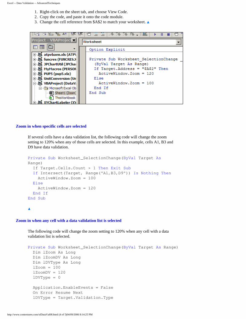
Zoom in when specific cell is selected
If cell A2 has a data validation list, the following code will change the zoom setting to 120% when that cell is selected.
Private Sub Worksheet_SelectionChange(ByVal Target As Range) If Target.Address = "$A$2" Then ActiveWindow.Zoom = 120 Else ActiveWindow.Zoom = 100 End If End Sub
To add this code to the worksheet:
http://www.contextures.com/xlDataVal08.html (3 of 5)04/09/2006 8:14:25 PM
Excel -- Data Validation -- AdvancedTechniques
1. Right-click on the sheet tab, and choose View Code. 2. Copy the code, and paste it onto the code module. 3. Change the cell reference from $A$2 to match your worksheet.
Zoom in when specific cells are selected
If several cells have a data validation list, the following code will change the zoom setting to 120% when any of those cells are selected. In this example, cells A1, B3 and D9 have data validation.
Private Sub Worksheet_SelectionChange(ByVal Target As Range) If Target.Cells.Count > 1 Then Exit Sub If Intersect(Target, Range("A1,B3,D9")) Is Nothing Then ActiveWindow.Zoom = 100 Else ActiveWindow.Zoom = 120 End If End Sub
Zoom in when any cell with a data validation list is selected
The following code will change the zoom setting to 120% when any cell with a data validation list is selected.
Private Sub Worksheet_SelectionChange(ByVal Target As Range) Dim lZoom As Long Dim lZoomDV As Long Dim lDVType As Long lZoom = 100 lZoomDV = 120 lDVType = 0
Application.EnableEvents = False On Error Resume Next lDVType = Target.Validation.Type
http://www.contextures.com/xlDataVal08.html (4 of 5)04/09/2006 8:14:25 PM
Excel -- Data Validation -- AdvancedTechniques
On Error GoTo errHandler If lDVType <> 3 Then With ActiveWindow If .Zoom <> lZoom Then .Zoom = lZoom End If End With Else With ActiveWindow If .Zoom <> lZoomDV Then .Zoom = lZoomDV End If End With End If
exitHandler: Application.EnableEvents = True Exit SuberrHandler: GoTo exitHandlerEnd Sub
1. Data Validation2. Data Validation -- Create Dependent Lists3. Hide Previously Used Items in a Dropdown List4. Display Messages to the User5. Use a List from Another Workbook 6. Validation Criteria Examples 7. Custom Validation Criteria Examples8. Data Validation Tips9. Data Validation Documentation 10 Data Validation -- Combo box 11. Data Validation -- Combo Box - Named Ranges 12. Data Validation -- Display Input Messages in a Text Box 13. Data Validation -- Dependent Dropdowns from a Sorted List
Home Excel Tips Sample Spreadsheets
Contextures contact information
Last updated: June 4, 2006 11:22 AM
http://www.contextures.com/xlDataVal08.html (5 of 5)04/09/2006 8:14:25 PM
Excel -- Data Validation -- Documentation
Home Excel Tips Sample Spreadsheets
Excel -- Data Validation -- Documentation
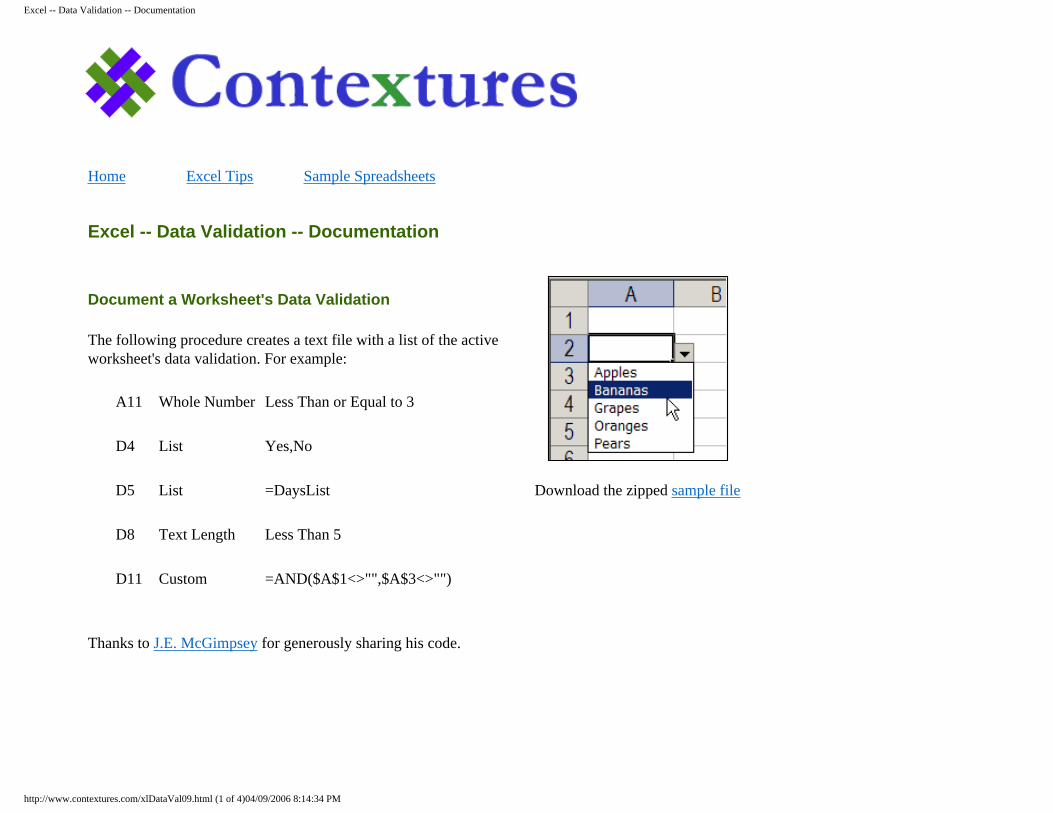
Document a Worksheet's Data Validation
The following procedure creates a text file with a list of the active worksheet's data validation. For example:
A11 Whole Number Less Than or Equal to 3
D4 List Yes,No
D5 List =DaysList
D8 Text Length Less Than 5
D11 Custom =AND($A$1<>"",$A$3<>"")
Thanks to J.E. McGimpsey for generously sharing his code.
Download the zipped sample file
http://www.contextures.com/xlDataVal09.html (1 of 4)04/09/2006 8:14:34 PM
Excel -- Data Validation -- Documentation
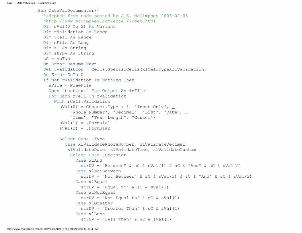
Sub DataValDocumenter() 'adapted from code posted by J.E. McGimpsey 2005-02-03 'http://www.mcgimpsey.com/excel/index.html Dim sVal(0 To 2) As Variant Dim rValidation As Range Dim rCell As Range Dim nFile As Long Dim sC As String Dim strDV As String sC = vbTab On Error Resume Next Set rValidation = Cells.SpecialCells(xlCellTypeAllValidation) On Error GoTo 0 If Not rValidation Is Nothing Then nFile = FreeFile Open "test.txt" For Output As #nFile For Each rCell In rValidation With rCell.Validation sVal(0) = Choose(.Type + 1, "Input Only", _ "Whole Number", "Decimal", "List", "Date", _ "Time", "Text Length", "Custom") sVal(1) = .Formula1 sVal(2) = .Formula2
Select Case .Type Case xlValidateWholeNumber, xlValidateDecimal, _ xlValidateDate, xlValidateTime, xlValidateCustom Select Case .Operator Case xlAnd strDV = "Between" & sC & sVal(1) & sC & "And" & sC & sVal(2) Case xlNotBetween strDV = "Not Between" & sC & sVal(1) & sC & "And" & sC & sVal(2) Case xlEqual strDV = "Equal to" & sC & sVal(1) Case xlNotEqual strDV = "Not Equal to" & sC & sVal(1) Case xlGreater strDV = "Greater Than" & sC & sVal(1) Case xlLess strDV = "Less Than" & sC & sVal(1)
http://www.contextures.com/xlDataVal09.html (2 of 4)04/09/2006 8:14:34 PM
Excel -- Data Validation -- Documentation
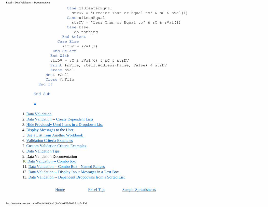
Case xlGreaterEqual strDV = "Greater Than or Equal to" & sC & sVal(1) Case xlLessEqual strDV = "Less Than or Equal to" & sC & sVal(1) Case Else 'do nothing End Select Case Else strDV = sVal(1) End Select End With strDV = sC & sVal(0) & sC & strDV Print #nFile, rCell.Address(False, False) & strDV Erase sVal Next rCell Close #nFile End If
End Sub
1. Data Validation2. Data Validation -- Create Dependent Lists3. Hide Previously Used Items in a Dropdown List4. Display Messages to the User5. Use a List from Another Workbook 6. Validation Criteria Examples 7. Custom Validation Criteria Examples8. Data Validation Tips9. Data Validation Documentation 10 Data Validation -- Combo box 11. Data Validation -- Combo Box - Named Ranges 12. Data Validation -- Display Input Messages in a Text Box 13. Data Validation -- Dependent Dropdowns from a Sorted List
Home Excel Tips Sample Spreadsheets
http://www.contextures.com/xlDataVal09.html (3 of 4)04/09/2006 8:14:34 PM
Excel -- Data Validation -- Documentation
Contextures contact information
Last updated: June 4, 2006 11:30 AM
http://www.contextures.com/xlDataVal09.html (4 of 4)04/09/2006 8:14:34 PM
Excel -- Data Validation -- Combo box
Home Excel Tips Sample Spreadsheets
Excel -- Data Validation -- Combo box
Create a Data Validation Dropdown List Add the Combo box Open the Properties Window Change the Combo box Properties Exit Design Mode Add the Code Test the Code
Download the zipped sample file
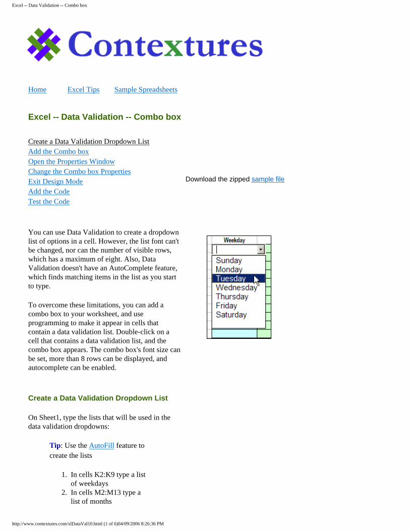
You can use Data Validation to create a dropdown list of options in a cell. However, the list font can't be changed, nor can the number of visible rows, which has a maximum of eight. Also, Data Validation doesn't have an AutoComplete feature, which finds matching items in the list as you start to type.
To overcome these limitations, you can add a combo box to your worksheet, and use programming to make it appear in cells that contain a data validation list. Double-click on a cell that contains a data validation list, and the combo box appears. The combo box's font size can be set, more than 8 rows can be displayed, and autocomplete can be enabled.
Create a Data Validation Dropdown List
On Sheet1, type the lists that will be used in the data validation dropdowns:
Tip: Use the AutoFill feature to create the lists
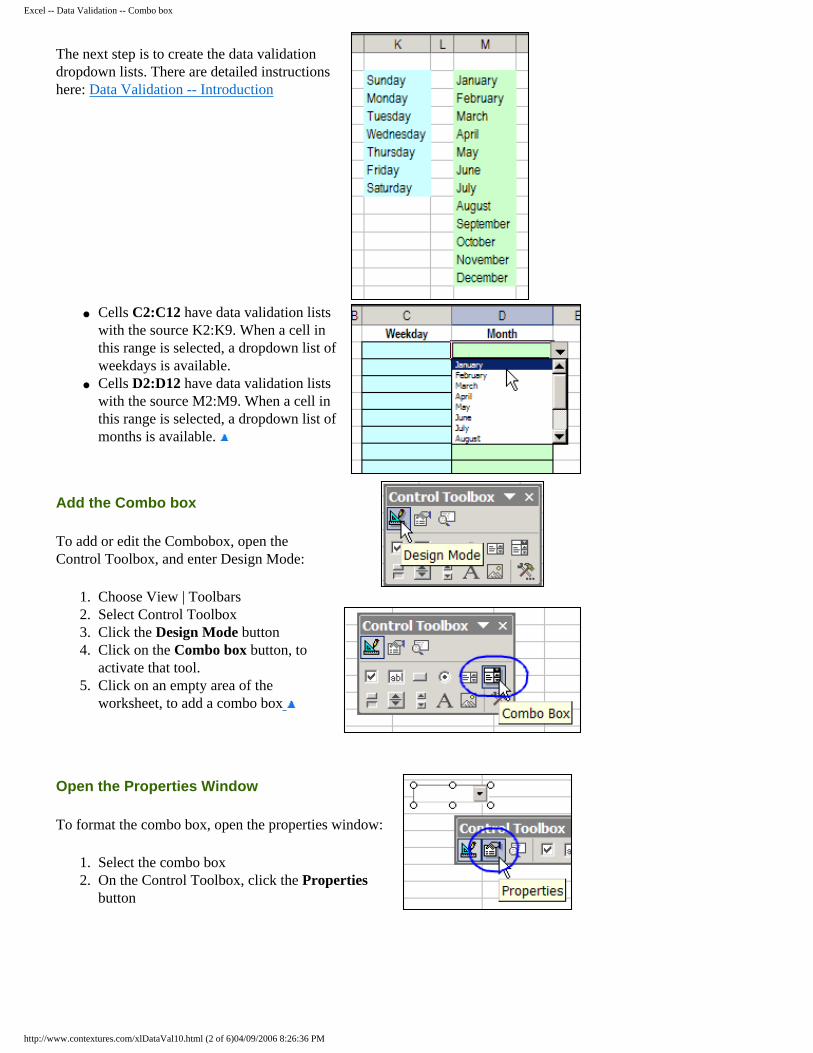
1. In cells K2:K9 type a list of weekdays
2. In cells M2:M13 type a list of months
http://www.contextures.com/xlDataVal10.html (1 of 6)04/09/2006 8:26:36 PM
Excel -- Data Validation -- Combo box
The next step is to create the data validation dropdown lists. There are detailed instructions here: Data Validation -- Introduction
● Cells C2:C12 have data validation lists with the source K2:K9. When a cell in this range is selected, a dropdown list of weekdays is available.
● Cells D2:D12 have data validation lists with the source M2:M9. When a cell in this range is selected, a dropdown list of months is available.
Add the Combo box
To add or edit the Combobox, open the Control Toolbox, and enter Design Mode:
1. Choose View | Toolbars2. Select Control Toolbox 3. Click the Design Mode button4. Click on the Combo box button, to
activate that tool.5. Click on an empty area of the
worksheet, to add a combo box
Open the Properties Window
To format the combo box, open the properties window:
1. Select the combo box2. On the Control Toolbox, click the Properties
button
http://www.contextures.com/xlDataVal10.html (2 of 6)04/09/2006 8:26:36 PM
Excel -- Data Validation -- Combo box
Change the Combo box Properties
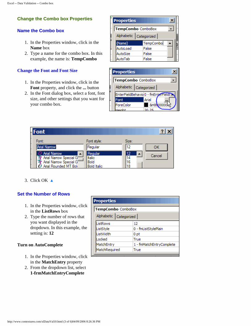
Name the Combo box
1. In the Properties window, click in the Name box
2. Type a name for the combo box. In this example, the name is: TempCombo
Change the Font and Font Size
1. In the Properties window, click in the Font property, and click the ... button
2. In the Font dialog box, select a font, font size, and other settings that you want for your combo box.
3. Click OK
Set the Number of Rows
1. In the Properties window, click in the ListRows box
2. Type the number of rows that you want displayed in the dropdown. In this example, the setting is: 12
Turn on AutoComplete
1. In the Properties window, click in the MatchEntry property
2. From the dropdown list, select 1-frmMatchEntryComplete
http://www.contextures.com/xlDataVal10.html (3 of 6)04/09/2006 8:26:36 PM
Excel -- Data Validation -- Combo box
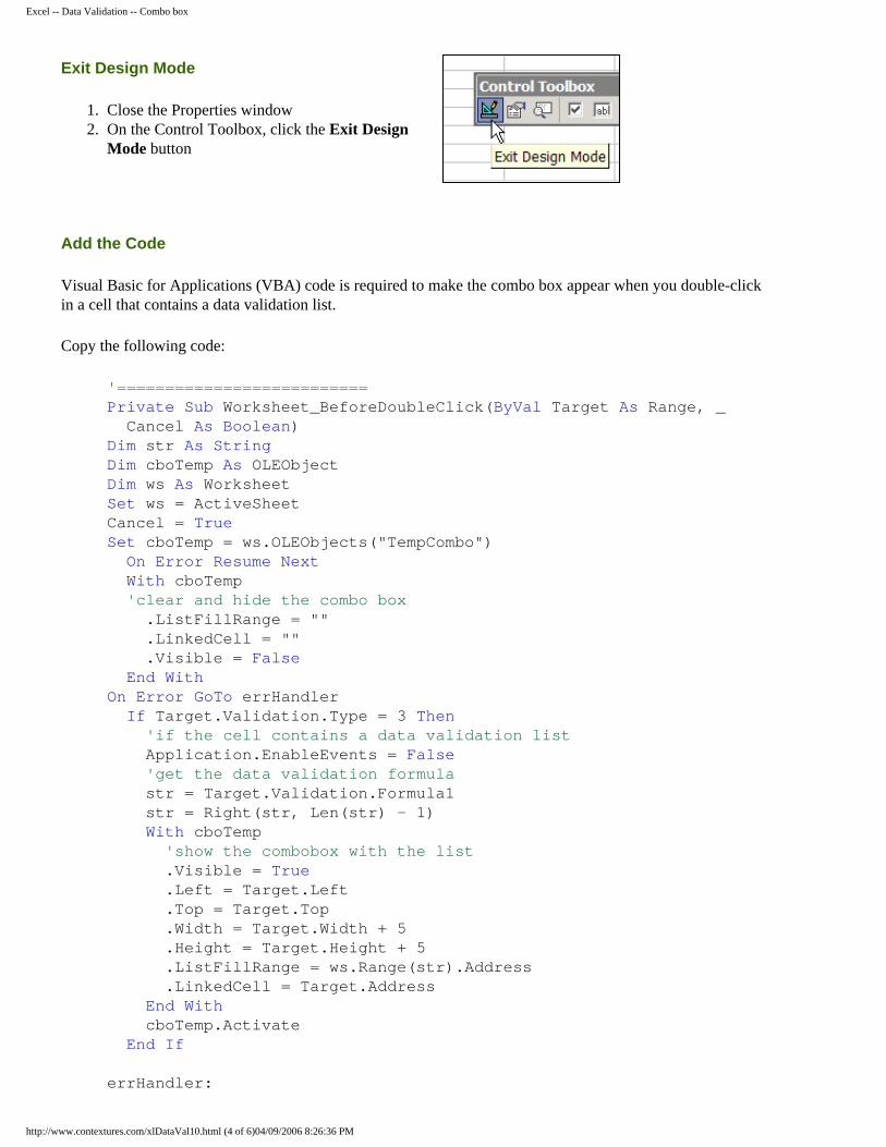
Exit Design Mode
1. Close the Properties window2. On the Control Toolbox, click the Exit Design
Mode button
Add the Code
Visual Basic for Applications (VBA) code is required to make the combo box appear when you double-click in a cell that contains a data validation list.
Copy the following code:
'==========================Private Sub Worksheet_BeforeDoubleClick(ByVal Target As Range, _ Cancel As Boolean)Dim str As StringDim cboTemp As OLEObjectDim ws As WorksheetSet ws = ActiveSheetCancel = TrueSet cboTemp = ws.OLEObjects("TempCombo") On Error Resume Next With cboTemp 'clear and hide the combo box .ListFillRange = "" .LinkedCell = "" .Visible = False End WithOn Error GoTo errHandler If Target.Validation.Type = 3 Then 'if the cell contains a data validation list Application.EnableEvents = False 'get the data validation formula str = Target.Validation.Formula1 str = Right(str, Len(str) - 1) With cboTemp 'show the combobox with the list .Visible = True .Left = Target.Left .Top = Target.Top .Width = Target.Width + 5 .Height = Target.Height + 5 .ListFillRange = ws.Range(str).Address .LinkedCell = Target.Address End With cboTemp.Activate End If errHandler:
http://www.contextures.com/xlDataVal10.html (4 of 6)04/09/2006 8:26:36 PM
Excel -- Data Validation -- Combo box
Application.EnableEvents = True Exit Sub
End Sub'=========================================Private Sub Worksheet_SelectionChange(ByVal Target As Range)Dim str As StringDim cboTemp As OLEObjectDim ws As WorksheetSet ws = ActiveSheet
Set cboTemp = ws.OLEObjects("TempCombo") On Error Resume NextIf cboTemp.Visible = True Then With cboTemp .Top = 10 .Left = 10 .ListFillRange = "" .LinkedCell = "" .Visible = False .Value = "" End WithEnd If
errHandler: Application.EnableEvents = True Exit Sub
End Sub '====================================
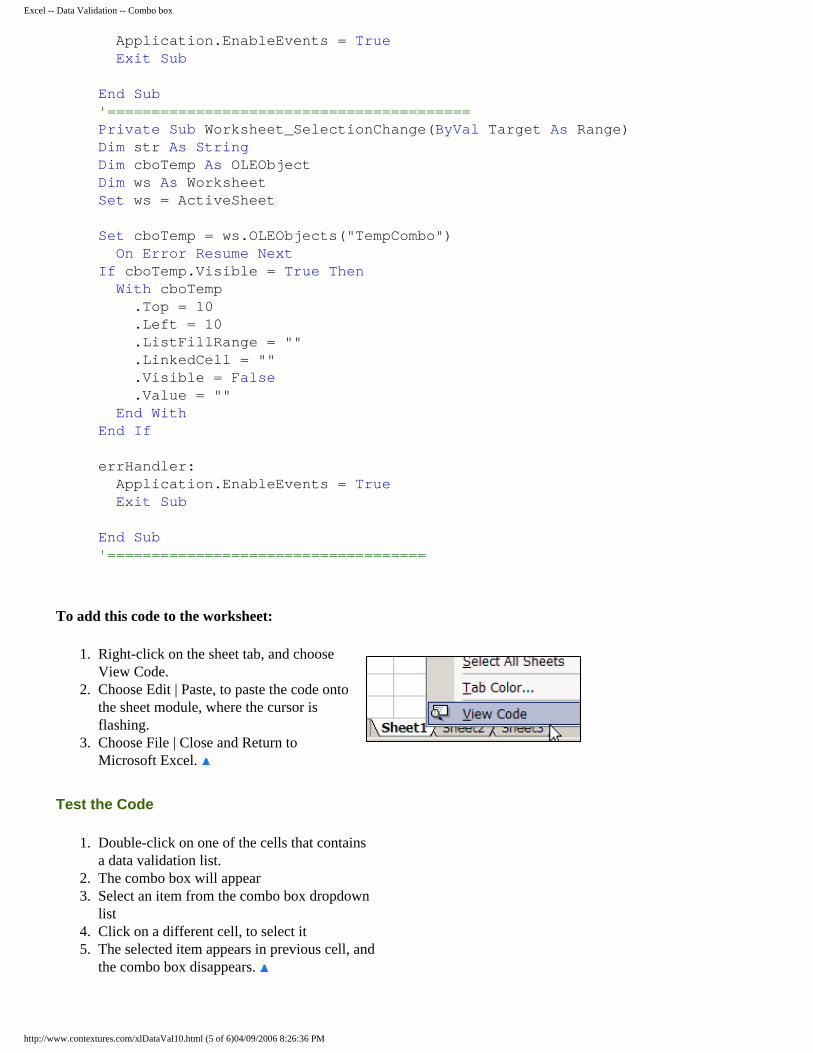
To add this code to the worksheet:
1. Right-click on the sheet tab, and choose View Code.
2. Choose Edit | Paste, to paste the code onto the sheet module, where the cursor is flashing.
3. Choose File | Close and Return to Microsoft Excel.
Test the Code
1. Double-click on one of the cells that contains a data validation list.
2. The combo box will appear3. Select an item from the combo box dropdown
list4. Click on a different cell, to select it5. The selected item appears in previous cell, and
the combo box disappears.
http://www.contextures.com/xlDataVal10.html (5 of 6)04/09/2006 8:26:36 PM
Excel -- Data Validation -- Combo box
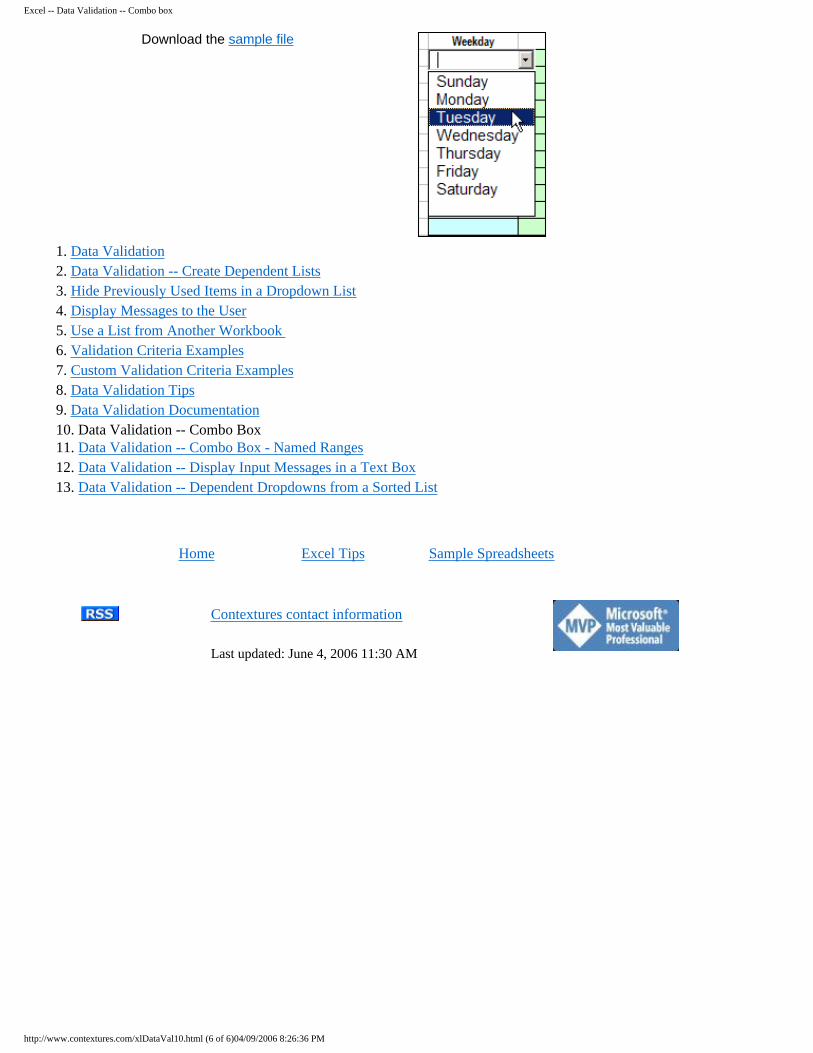
Download the sample file
1. Data Validation2. Data Validation -- Create Dependent Lists3. Hide Previously Used Items in a Dropdown List4. Display Messages to the User5. Use a List from Another Workbook 6. Validation Criteria Examples 7. Custom Validation Criteria Examples8. Data Validation Tips9. Data Validation Documentation10. Data Validation -- Combo Box 11. Data Validation -- Combo Box - Named Ranges 12. Data Validation -- Display Input Messages in a Text Box 13. Data Validation -- Dependent Dropdowns from a Sorted List
Home Excel Tips Sample Spreadsheets
Contextures contact information
Last updated: June 4, 2006 11:30 AM
http://www.contextures.com/xlDataVal10.html (6 of 6)04/09/2006 8:26:36 PM
Excel -- Data Validation -- Combo box using Named Ranges
Home Excel Tips Sample Spreadsheets
Excel -- Data Validation -- Combo box using Named Ranges
Set up the Workbook Create a Data Validation Dropdown List Add the Combo box Open the Properties Window Change the Combo box Properties Exit Design Mode Add the Code Test the Code
Download the zipped sample file
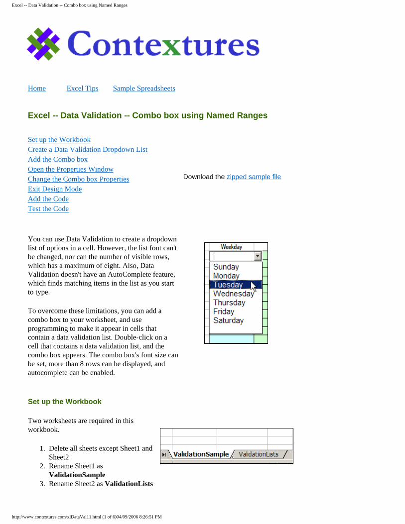
You can use Data Validation to create a dropdown list of options in a cell. However, the list font can't be changed, nor can the number of visible rows, which has a maximum of eight. Also, Data Validation doesn't have an AutoComplete feature, which finds matching items in the list as you start to type.
To overcome these limitations, you can add a combo box to your worksheet, and use programming to make it appear in cells that contain a data validation list. Double-click on a cell that contains a data validation list, and the combo box appears. The combo box's font size can be set, more than 8 rows can be displayed, and autocomplete can be enabled.
Set up the Workbook
Two worksheets are required in this workbook.
1. Delete all sheets except Sheet1 and Sheet2
2. Rename Sheet1 as ValidationSample
3. Rename Sheet2 as ValidationLists
http://www.contextures.com/xlDataVal11.html (1 of 6)04/09/2006 8:26:51 PM
Excel -- Data Validation -- Combo box using Named Ranges
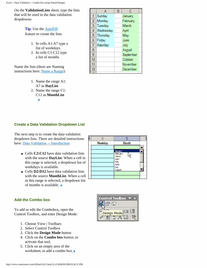
On the ValidationLists sheet, type the lists that will be used in the data validation dropdowns:
Tip: Use the AutoFill feature to create the lists
1. In cells A1:A7 type a list of weekdays
2. In cells C1:C12 type a list of months
Name the lists (there are Naming instructions here: Name a Range):
1. Name the range A1:A7 as DayList
2. Name the range C1:C12 as MonthList
Create a Data Validation Dropdown List
The next step is to create the data validation dropdown lists. There are detailed instructions here: Data Validation -- Introduction
● Cells C2:C12 have data validation lists with the source DayList. When a cell in this range is selected, a dropdown list of weekdays is available.
● Cells D2:D12 have data validation lists with the source MonthList. When a cell in this range is selected, a dropdown list of months is available.
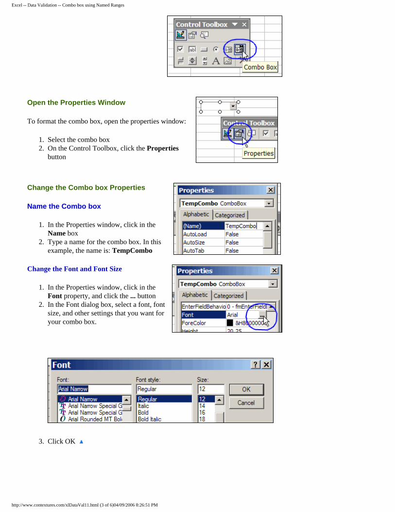
Add the Combo box
To add or edit the Combobox, open the Control Toolbox, and enter Design Mode:
1. Choose View | Toolbars2. Select Control Toolbox 3. Click the Design Mode button4. Click on the Combo box button, to
activate that tool.5. Click on an empty area of the
worksheet, to add a combo box
http://www.contextures.com/xlDataVal11.html (2 of 6)04/09/2006 8:26:51 PM
Excel -- Data Validation -- Combo box using Named Ranges
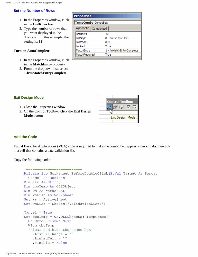
Open the Properties Window
To format the combo box, open the properties window:
1. Select the combo box2. On the Control Toolbox, click the Properties
button
Change the Combo box Properties
Name the Combo box
1. In the Properties window, click in the Name box
2. Type a name for the combo box. In this example, the name is: TempCombo
Change the Font and Font Size
1. In the Properties window, click in the Font property, and click the ... button
2. In the Font dialog box, select a font, font size, and other settings that you want for your combo box.
3. Click OK
http://www.contextures.com/xlDataVal11.html (3 of 6)04/09/2006 8:26:51 PM
Excel -- Data Validation -- Combo box using Named Ranges
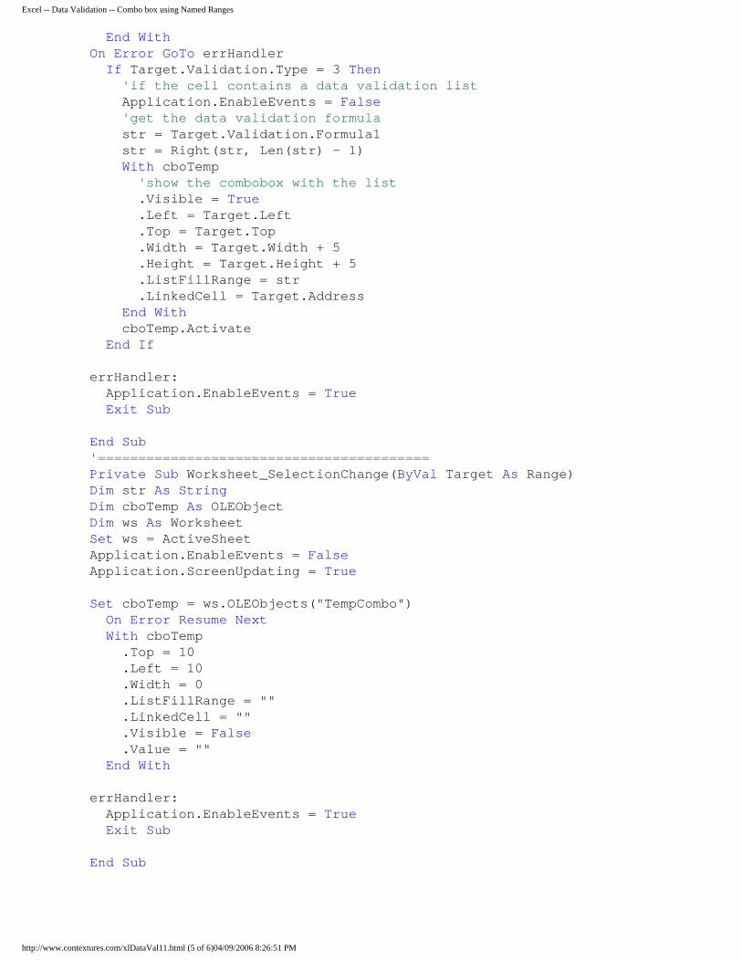
Set the Number of Rows
1. In the Properties window, click in the ListRows box
2. Type the number of rows that you want displayed in the dropdown. In this example, the setting is: 12
Turn on AutoComplete
1. In the Properties window, click in the MatchEntry property
2. From the dropdown list, select 1-frmMatchEntryComplete
Exit Design Mode
1. Close the Properties window2. On the Control Toolbox, click the Exit Design
Mode button
Add the Code
Visual Basic for Applications (VBA) code is required to make the combo box appear when you double-click in a cell that contains a data validation list.
Copy the following code:
'==========================Private Sub Worksheet_BeforeDoubleClick(ByVal Target As Range, _ Cancel As Boolean)Dim str As StringDim cboTemp As OLEObjectDim ws As WorksheetDim wsList As WorksheetSet ws = ActiveSheetSet wsList = Sheets("ValidationLists")
Cancel = TrueSet cboTemp = ws.OLEObjects("TempCombo") On Error Resume Next With cboTemp 'clear and hide the combo box .ListFillRange = "" .LinkedCell = "" .Visible = False
http://www.contextures.com/xlDataVal11.html (4 of 6)04/09/2006 8:26:51 PM
Excel -- Data Validation -- Combo box using Named Ranges
End WithOn Error GoTo errHandler If Target.Validation.Type = 3 Then 'if the cell contains a data validation list Application.EnableEvents = False 'get the data validation formula str = Target.Validation.Formula1 str = Right(str, Len(str) - 1) With cboTemp 'show the combobox with the list .Visible = True .Left = Target.Left .Top = Target.Top .Width = Target.Width + 5 .Height = Target.Height + 5 .ListFillRange = str .LinkedCell = Target.Address End With cboTemp.Activate End If errHandler: Application.EnableEvents = True Exit Sub
End Sub'=========================================Private Sub Worksheet_SelectionChange(ByVal Target As Range)Dim str As StringDim cboTemp As OLEObjectDim ws As WorksheetSet ws = ActiveSheetApplication.EnableEvents = FalseApplication.ScreenUpdating = True
Set cboTemp = ws.OLEObjects("TempCombo") On Error Resume Next With cboTemp .Top = 10 .Left = 10 .Width = 0 .ListFillRange = "" .LinkedCell = "" .Visible = False .Value = "" End With
errHandler: Application.EnableEvents = True Exit Sub
End Sub
http://www.contextures.com/xlDataVal11.html (5 of 6)04/09/2006 8:26:51 PM
Excel -- Data Validation -- Combo box using Named Ranges
To add this code to the worksheet:
1. Right-click on the sheet tab, and choose View Code.
2. Choose Edit | Paste, to paste the code onto the sheet module, where the cursor is flashing.
3. Choose File | Close and Return to Microsoft Excel.
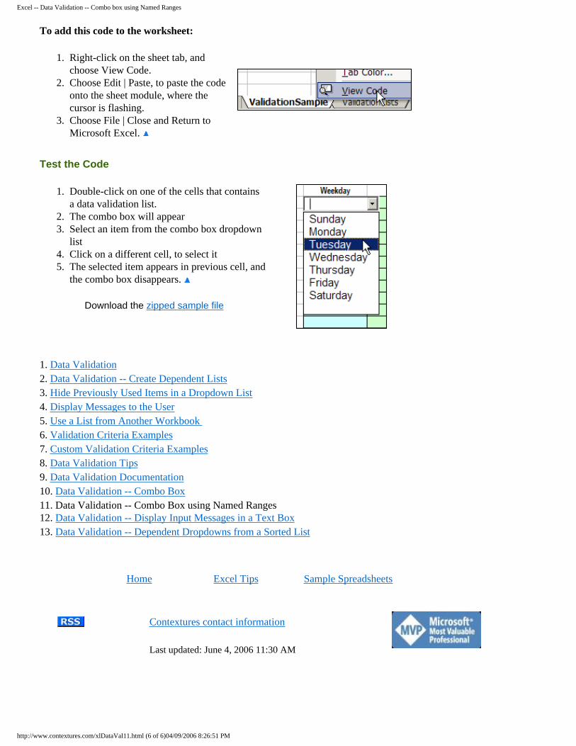
Test the Code
1. Double-click on one of the cells that contains a data validation list.
2. The combo box will appear3. Select an item from the combo box dropdown
list4. Click on a different cell, to select it5. The selected item appears in previous cell, and
the combo box disappears.
Download the zipped sample file
1. Data Validation2. Data Validation -- Create Dependent Lists3. Hide Previously Used Items in a Dropdown List4. Display Messages to the User5. Use a List from Another Workbook 6. Validation Criteria Examples 7. Custom Validation Criteria Examples8. Data Validation Tips9. Data Validation Documentation10. Data Validation -- Combo Box 11. Data Validation -- Combo Box using Named Ranges 12. Data Validation -- Display Input Messages in a Text Box 13. Data Validation -- Dependent Dropdowns from a Sorted List
Home Excel Tips Sample Spreadsheets
Contextures contact information
Last updated: June 4, 2006 11:30 AM
http://www.contextures.com/xlDataVal11.html (6 of 6)04/09/2006 8:26:51 PM
Excel -- Data Validation -- Display Input Messages in a Textbox
Home Excel Tips Sample Spreadsheets
Excel -- Data Validation -- Display Input Messages in a Text Box
Set up the Workbook Create a Data Validation Dropdown List Add the Text Box Name the Text Box Add the Code Test the Code
Download the zipped sample file
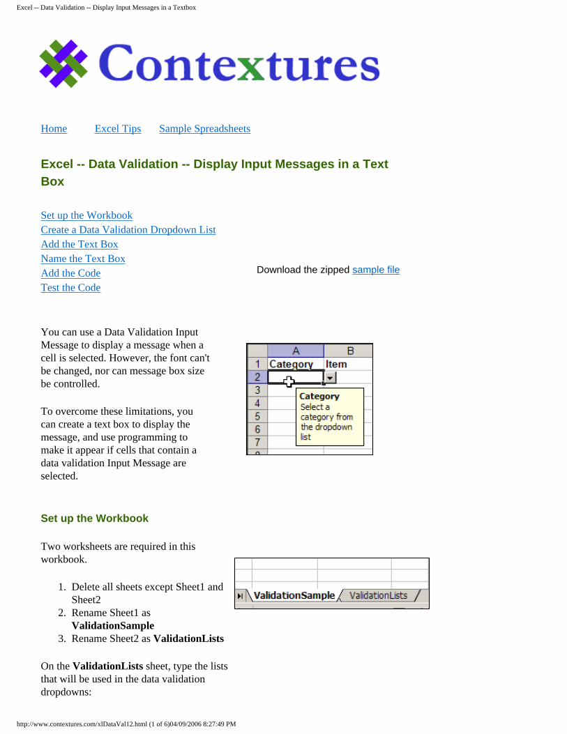
You can use a Data Validation Input Message to display a message when a cell is selected. However, the font can't be changed, nor can message box size be controlled.
To overcome these limitations, you can create a text box to display the message, and use programming to make it appear if cells that contain a data validation Input Message are selected.
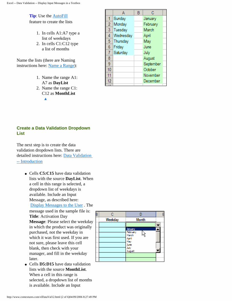
Set up the Workbook
Two worksheets are required in this workbook.
1. Delete all sheets except Sheet1 and Sheet2
2. Rename Sheet1 as ValidationSample
3. Rename Sheet2 as ValidationLists
On the ValidationLists sheet, type the lists that will be used in the data validation dropdowns:
http://www.contextures.com/xlDataVal12.html (1 of 6)04/09/2006 8:27:49 PM
Excel -- Data Validation -- Display Input Messages in a Textbox
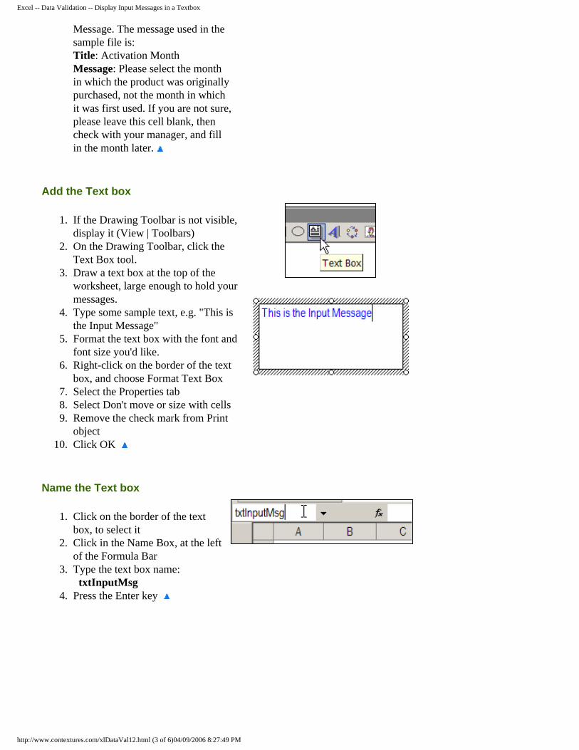
Tip: Use the AutoFill feature to create the lists
1. In cells A1:A7 type a list of weekdays
2. In cells C1:C12 type a list of months
Name the lists (there are Naming instructions here: Name a Range):
1. Name the range A1:A7 as DayList
2. Name the range C1:C12 as MonthList
Create a Data Validation Dropdown List
The next step is to create the data validation dropdown lists. There are detailed instructions here: Data Validation -- Introduction
● Cells C5:C15 have data validation lists with the source DayList. When a cell in this range is selected, a dropdown list of weekdays is available. Include an Input Message, as described here: Display Messages to the User . The message used in the sample file is:Title: Activation Day Message: Please select the weekday in which the product was originally purchased, not the weekday in which it was first used. If you are not sure, please leave this cell blank, then check with your manager, and fill in the weekday later.
● Cells D5:D15 have data validation lists with the source MonthList. When a cell in this range is selected, a dropdown list of months is available. Include an Input
http://www.contextures.com/xlDataVal12.html (2 of 6)04/09/2006 8:27:49 PM
Excel -- Data Validation -- Display Input Messages in a Textbox
Message. The message used in the sample file is:Title: Activation Month Message: Please select the month in which the product was originally purchased, not the month in which it was first used. If you are not sure, please leave this cell blank, then check with your manager, and fill in the month later.
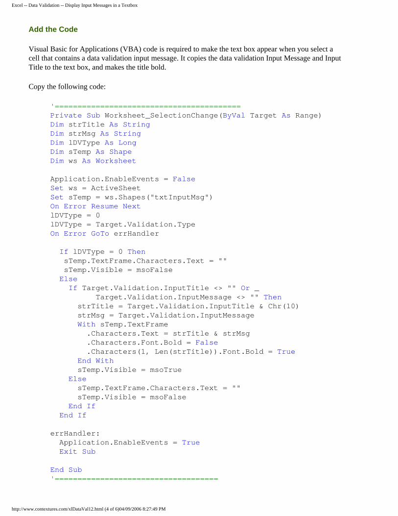
Add the Text box
1. If the Drawing Toolbar is not visible, display it (View | Toolbars)
2. On the Drawing Toolbar, click the Text Box tool.
3. Draw a text box at the top of the worksheet, large enough to hold your messages.
4. Type some sample text, e.g. "This is the Input Message"
5. Format the text box with the font and font size you'd like.
6. Right-click on the border of the text box, and choose Format Text Box
7. Select the Properties tab8. Select Don't move or size with cells9. Remove the check mark from Print
object10. Click OK
Name the Text box
1. Click on the border of the text box, to select it
2. Click in the Name Box, at the left of the Formula Bar
3. Type the text box name: txtInputMsg
4. Press the Enter key
http://www.contextures.com/xlDataVal12.html (3 of 6)04/09/2006 8:27:49 PM
Excel -- Data Validation -- Display Input Messages in a Textbox
Add the Code
Visual Basic for Applications (VBA) code is required to make the text box appear when you select a cell that contains a data validation input message. It copies the data validation Input Message and Input Title to the text box, and makes the title bold.
Copy the following code:
'=========================================Private Sub Worksheet_SelectionChange(ByVal Target As Range)Dim strTitle As StringDim strMsg As StringDim lDVType As LongDim sTemp As ShapeDim ws As Worksheet
Application.EnableEvents = FalseSet ws = ActiveSheetSet sTemp = ws.Shapes("txtInputMsg")On Error Resume NextlDVType = 0lDVType = Target.Validation.TypeOn Error GoTo errHandler
If lDVType = 0 Then sTemp.TextFrame.Characters.Text = "" sTemp.Visible = msoFalse Else If Target.Validation.InputTitle <> "" Or _ Target.Validation.InputMessage <> "" Then strTitle = Target.Validation.InputTitle & Chr(10) strMsg = Target.Validation.InputMessage With sTemp.TextFrame .Characters.Text = strTitle & strMsg .Characters.Font.Bold = False .Characters(1, Len(strTitle)).Font.Bold = True End With sTemp.Visible = msoTrue Else sTemp.TextFrame.Characters.Text = "" sTemp.Visible = msoFalse End If End If
errHandler: Application.EnableEvents = True Exit Sub
End Sub '====================================
http://www.contextures.com/xlDataVal12.html (4 of 6)04/09/2006 8:27:49 PM
Excel -- Data Validation -- Display Input Messages in a Textbox
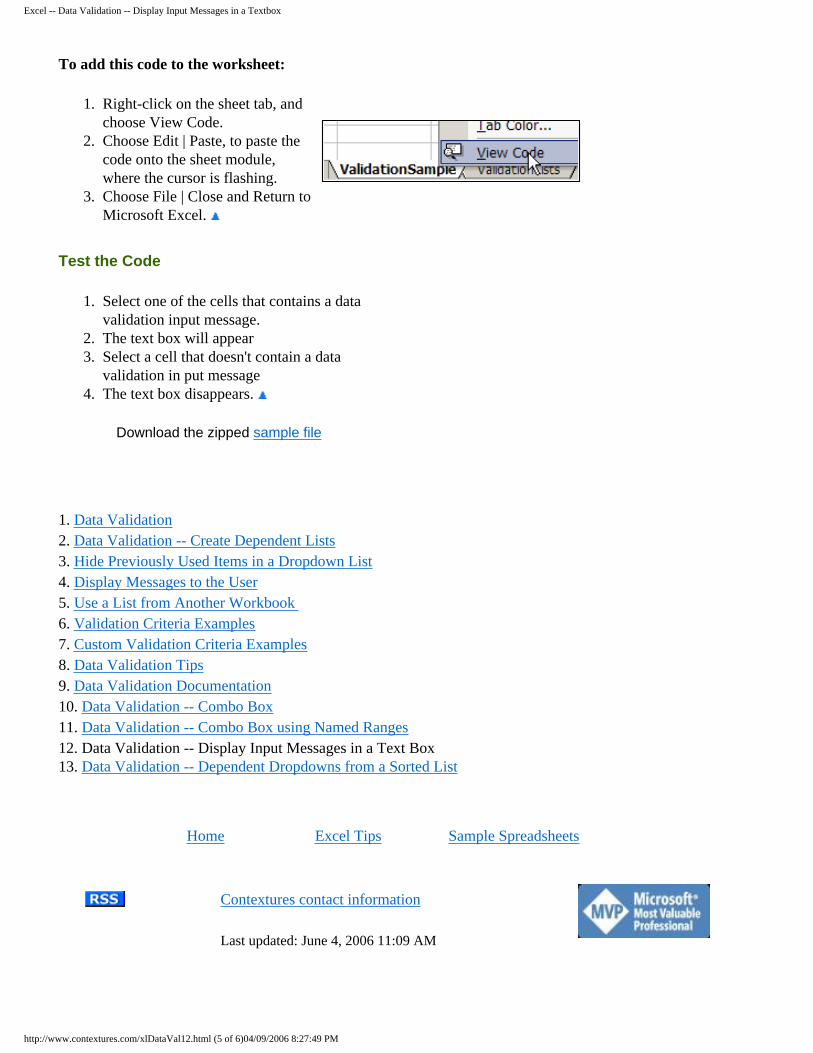
To add this code to the worksheet:
1. Right-click on the sheet tab, and choose View Code.
2. Choose Edit | Paste, to paste the code onto the sheet module, where the cursor is flashing.
3. Choose File | Close and Return to Microsoft Excel.
Test the Code
1. Select one of the cells that contains a data validation input message.
2. The text box will appear3. Select a cell that doesn't contain a data
validation in put message4. The text box disappears.
Download the zipped sample file
1. Data Validation2. Data Validation -- Create Dependent Lists3. Hide Previously Used Items in a Dropdown List4. Display Messages to the User5. Use a List from Another Workbook 6. Validation Criteria Examples 7. Custom Validation Criteria Examples8. Data Validation Tips9. Data Validation Documentation10. Data Validation -- Combo Box 11. Data Validation -- Combo Box using Named Ranges 12. Data Validation -- Display Input Messages in a Text Box 13. Data Validation -- Dependent Dropdowns from a Sorted List
Home Excel Tips Sample Spreadsheets
Contextures contact information
Last updated: June 4, 2006 11:09 AM
http://www.contextures.com/xlDataVal12.html (5 of 6)04/09/2006 8:27:49 PM

Excel -- Data Validation -- Display Input Messages in a Textbox
http://www.contextures.com/xlDataVal12.html (6 of 6)04/09/2006 8:27:49 PM
Excel -- Data Validation -- Dependent Dropdowns from a Sorted List
Home Excel Tips Sample Spreadsheets
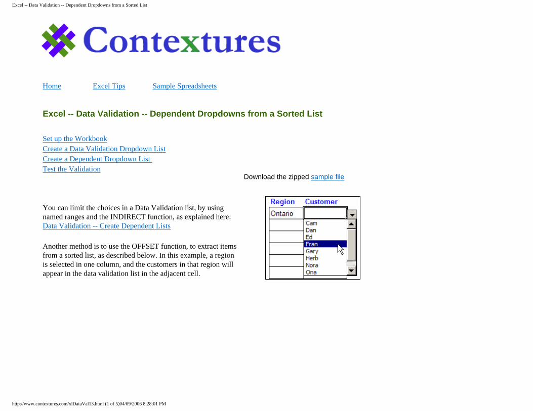
Excel -- Data Validation -- Dependent Dropdowns from a Sorted List
Set up the Workbook Create a Data Validation Dropdown List Create a Dependent Dropdown List Test the Validation
Download the zipped sample file
You can limit the choices in a Data Validation list, by using named ranges and the INDIRECT function, as explained here: Data Validation -- Create Dependent Lists
Another method is to use the OFFSET function, to extract items from a sorted list, as described below. In this example, a region is selected in one column, and the customers in that region will appear in the data validation list in the adjacent cell.
http://www.contextures.com/xlDataVal13.html (1 of 5)04/09/2006 8:28:01 PM
Excel -- Data Validation -- Dependent Dropdowns from a Sorted List
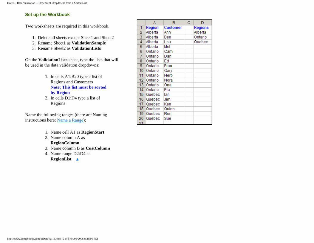
Set up the Workbook
Two worksheets are required in this workbook.
1. Delete all sheets except Sheet1 and Sheet22. Rename Sheet1 as ValidationSample3. Rename Sheet2 as ValidationLists
On the ValidationLists sheet, type the lists that will be used in the data validation dropdowns:
1. In cells A1:B20 type a list of Regions and Customers Note: This list must be sorted by Region
2. In cells D1:D4 type a list of Regions
Name the following ranges (there are Naming instructions here: Name a Range):
1. Name cell A1 as RegionStart2. Name column A as
RegionColumn3. Name column B as CustColumn4. Name range D2:D4 as
RegionList
http://www.contextures.com/xlDataVal13.html (2 of 5)04/09/2006 8:28:01 PM
Excel -- Data Validation -- Dependent Dropdowns from a Sorted List
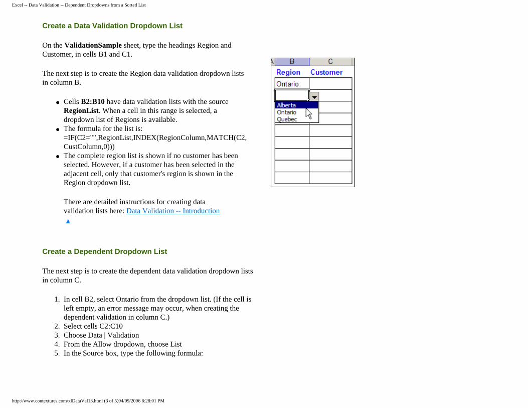
Create a Data Validation Dropdown List
On the ValidationSample sheet, type the headings Region and Customer, in cells B1 and C1.
The next step is to create the Region data validation dropdown lists in column B.
● Cells B2:B10 have data validation lists with the source RegionList. When a cell in this range is selected, a dropdown list of Regions is available.
● The formula for the list is:=IF(C2="",RegionList,INDEX(RegionColumn,MATCH(C2,CustColumn,0)))
● The complete region list is shown if no customer has been selected. However, if a customer has been selected in the adjacent cell, only that customer's region is shown in the Region dropdown list.
There are detailed instructions for creating data validation lists here: Data Validation -- Introduction
Create a Dependent Dropdown List
The next step is to create the dependent data validation dropdown lists in column C.
1. In cell B2, select Ontario from the dropdown list. (If the cell is left empty, an error message may occur, when creating the dependent validation in column C.)
2. Select cells C2:C103. Choose Data | Validation4. From the Allow dropdown, choose List5. In the Source box, type the following formula:
http://www.contextures.com/xlDataVal13.html (3 of 5)04/09/2006 8:28:01 PM
Excel -- Data Validation -- Dependent Dropdowns from a Sorted List
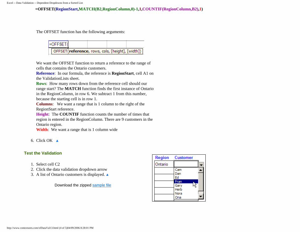
=OFFSET(RegionStart,MATCH(B2,RegionColumn,0)-1,1,COUNTIF(RegionColumn,B2),1)
The OFFSET function has the following arguments:
We want the OFFSET function to return a reference to the range of cells that contains the Ontario customers.Reference: In our formula, the reference is RegionStart, cell A1 on the ValidationLists sheet.Rows: How many rows down from the reference cell should our range start? The MATCH function finds the first instance of Ontario in the RegionColumn, in row 6. We subtract 1 from this number, because the starting cell is in row 1.Columns: We want a range that is 1 column to the right of the RegionStart reference.Height: The COUNTIF function counts the number of times that region is entered in the RegionColumn. There are 9 customers in the Ontario region. Width: We want a range that is 1 column wide
6. Click OK
Test the Validation
1. Select cell C22. Click the data validation dropdown arrow3. A list of Ontario customers is displayed.
Download the zipped sample file
http://www.contextures.com/xlDataVal13.html (4 of 5)04/09/2006 8:28:01 PM
Excel -- Data Validation -- Dependent Dropdowns from a Sorted List
1. Data Validation2. Data Validation -- Create Dependent Lists3. Hide Previously Used Items in a Dropdown List4. Display Messages to the User5. Use a List from Another Workbook 6. Validation Criteria Examples 7. Custom Validation Criteria Examples8. Data Validation Tips9. Data Validation Documentation10. Data Validation -- Combo Box 11. Data Validation -- Combo Box using Named Ranges 12. Data Validation -- Display Input Messages in a Text Box 13. Data Validation -- Dependent Dropdowns from a Sorted List
Home Excel Tips Sample Spreadsheets
Contextures contact information
Last updated: June 4, 2006 11:27 AM
http://www.contextures.com/xlDataVal13.html (5 of 5)04/09/2006 8:28:01 PM