
EvaluationandValidation - ls12-€¦ · EvaluationandValidation Jian%Jia&Chen (Slidesare&based&on&...
35
Evaluation and Validation JianJia Chen (Slides are based on Peter Marwedel) TU Dortmund, Informatik 12 Germany 2019年 11 月 27 日
Transcript of EvaluationandValidation - ls12-€¦ · EvaluationandValidation Jian%Jia&Chen (Slidesare&based&on&...

Evaluation and Validation
Jian-Jia Chen(Slides are based on Peter Marwedel)
TU Dortmund, Informatik 12Germany
2019年 11 月 27 日

- 2 -technische universitätdortmund
fakultät für informatik
© JJ Chen and P.Marwedel, Informatik 12, 2019
Structure of this course
2:Specification
3: ES-hardware
4: system software (RTOS, middleware, …)
8:Test
5: Evaluation & validation (energy, cost, performance, …)
7: Optimization
6: Application mapping
Application Knowledge Design repository Design
Numbers denote sequence of chapters

- 3 -technische universitätdortmund
fakultät für informatik
© JJ Chen and P.Marwedel, Informatik 12, 2019
Validation and Evaluation
Definition: Validation is the process of checking whether or not a certain (possibly partial) design is appropriate for its purpose, meets all constraints and will perform as expected (yes/no decision).
Definition: Validation with mathematical rigor is called (formal) verification.
Definition: Evaluation is the process of computing quantitative information of some key characteristics of a certain (possibly partial) design.

- 4 -technische universitätdortmund
fakultät für informatik
© JJ Chen and P.Marwedel, Informatik 12, 2019
How to evaluate designs according to multiple criteria?
Many different criteria are relevant for evaluating designs:§ Average & worst case delay§ power/energy consumption§ thermal behavior§ reliability, safety, security§ cost, size§ weight§ EMC characteristics§ radiation hardness, environmental friendliness, ..How to compare different designs?(Some designs are “better” than others)
- 5 -technische universitätdortmund
fakultät für informatik
© JJ Chen and P.Marwedel, Informatik 12, 2019
Definitions
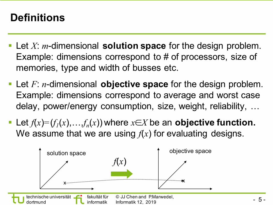
§ Let X: m-dimensional solution space for the design problem. Example: dimensions correspond to # of processors, size of memories, type and width of busses etc.
§ Let F: n-dimensional objective space for the design problem.Example: dimensions correspond to average and worst case delay, power/energy consumption, size, weight, reliability, …
§ Let f(x)=(f1(x),…,fn(x)) where x∈X be an objective function.We assume that we are using f(x) for evaluating designs.
solution space objective space
f(x)
x x

- 6 -technische universitätdortmund
fakultät für informatik
© JJ Chen and P.Marwedel, Informatik 12, 2019
Pareto points
ii
ii
vunivuni
<∈∃
∧≤∈∀
:,...,1:,...,1
§ We assume that, for each objective, an order < and the corresponding order ≤ are defined.
§ Definition:Vector u=(u1,…,un)∈ F dominates vector v=(v1,…,vn)∈ F⇔u is “better” than v with respect to at least one objective and not worse than v with respect to all other objectives:
§ Definition:Vector u∈ F is indifferent with respect to vector v∈ F⇔ neither u dominates v nor v dominates u

- 7 -technische universitätdortmund
fakultät für informatik
© JJ Chen and P.Marwedel, Informatik 12, 2019
Pareto points
§ A solution x∈X is called Pareto-optimal with respect to X⇔ there is no solution y∈X such that u=f(x) is dominated by v=f(y). x is a Pareto point.
§ Definition: Let S⊆ F be a subset of solutions.v∈ F is called a non-dominated solution with respect to S⇔ v is not dominated by any element ∈ S.
§ v is called Pareto-optimal⇔ v is non-dominated with respect to all solutions F.
§ A Pareto-set is the set of all Pareto-optimal solutions
Pareto-sets define a Pareto-front(boundary of dominated subspace)

- 8 -technische universitätdortmund
fakultät für informatik
© JJ Chen and P.Marwedel, Informatik 12, 2019
Pareto Point
Objective 1 (e.g. energyconsumption)
Objective 2(e.g. run time)
worse
better
Pareto-point
indifferent
indifferent
(Assuming minimization of objectives)

- 9 -technische universitätdortmund
fakultät für informatik
© JJ Chen and P.Marwedel, Informatik 12, 2019
Pareto Set
Objective 1 (e.g. energy consumption)
Objective 2(e.g. run time)
Pareto set = set of all Pareto-optimal solutions
dominated
Pareto-set
(Assuming minimization of objectives)

- 10 -technische universitätdortmund
fakultät für informatik
© JJ Chen and P.Marwedel, Informatik 12, 2019
One more time …
Pareto point Pareto front

- 11 -technische universitätdortmund
fakultät für informatik
© JJ Chen and P.Marwedel, Informatik 12, 2019
Design space evaluation
Design space evaluation (DSE) based on Pareto-points is the process of finding and returning a set of Pareto-optimal designs to the user, enabling the user to select the most appropriate design.

- 12 -technische universitätdortmund
fakultät für informatik
© JJ Chen and P.Marwedel, Informatik 12, 2019
How to evaluate designs according to multiple criteria?
Many different criteria are relevant for evaluating designs:§ Average & worst case delay§ power/energy consumption§ thermal behavior§ reliability, safety, security§ cost, size§ weight§ EMC characteristics§ radiation hardness, environmental friendliness, ..How to compare different designs?(Some designs are “better” than others)

- 13 -technische universitätdortmund
fakultät für informatik
© JJ Chen and P.Marwedel, Informatik 12, 2019
Average delays (execution times)
§ Estimated average execution times :Difficult to generate sufficiently precise estimates;;Balance between run-time and precision
§ Accurate average execution times:As precise as the input data is.
π x
We need to compute average and worst case execution times

- 14 -technische universitätdortmund
fakultät für informatik
© JJ Chen and P.Marwedel, Informatik 12, 2019
Worst case execution time (1)
Definition of worst case execution time:
WCET
EST
© Graphics: adopted fromR. Wilhelm + Microsoft Cliparts
WCETEST must be 1. safe (i.e. ≥ WCET) and2. tight (WCETEST-WCET≪WCETEST)
Timeconstraint
disrtribution of times
possible execution times
worst-case performanceworst-case guarantee
WCET
BCET
BCET
EST
timing predictability time

- 15 -technische universitätdortmund
fakultät für informatik
© JJ Chen and P.Marwedel, Informatik 12, 2019
Worst case execution times (2)
Complexity:§ in the general case: undecidable if a bound exists.§ for restricted programs: simple for “old“ architectures,very complex for new architectures with pipelines, caches, interrupts, virtual memory, etc.
Approaches: § for hardware: requires detailed timing behavior § for software: requires availability of machine programs;;complex analysis (see, e.g., www.absint.de)
- 16 -technische universitätdortmund
fakultät für informatik
© JJ Chen and P.Marwedel, Informatik 12, 2019
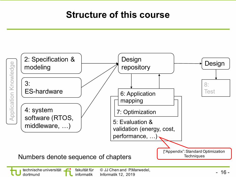
Structure of this course
2: Specification & modeling
3: ES-hardware
4: system software (RTOS, middleware, …)
8:Test
5: Evaluation & validation (energy, cost, performance, …)
7: Optimization
6: Application mapping
Application Knowledge Design repository Design
Numbers denote sequence of chapters[“Appendix”: Standard Optimization
Techniques

- 17 -technische universitätdortmund
fakultät für informatik
© JJ Chen and P.Marwedel, Informatik 12, 2019
Integer linear programming models
Ingredients:§ Cost function§ Constraints
Involving linear expressions of integer variables from a set X
Def.: The problem of minimizing (1) subject to the constraints (2) is called an integer linear programming (ILP) problem.
If all xi are constrained to be either 0 or 1, the ILP problem is said to be a 0/1 integer linear programming problem.
Cost function )1(,with NxRaxaC iXx
iiii
∈∈= ∑∈
Constraints: )2(,: ,, RcbcxbJjXx
jjijijii
∈≥∈∀ ∑∈
with
ℕ
ℝ
ℝ
ℝ

- 18 -technische universitätdortmund
fakultät für informatik
© JJ Chen and P.Marwedel, Informatik 12, 2019
Example
321 465 xxxC ++=
1,0,,2
321
321
∈
≥++
xxxxxx
Optimal
C

- 19 -technische universitätdortmund
fakultät für informatik
© JJ Chen and P.Marwedel, Informatik 12, 2019
Remarks on integer programming
§ Maximizing the cost function: just set C‘=-C§ Integer programming is NP-complete.§ Running times depend exponentially on problem size,but problems of >1000 vars solvable with good solver (depending on the size and structure of the problem)
§ The case of xi ∈ ℝ is called linear programming (LP).Polynomial complexity, but most algorithms are exponential, in practice still faster than for ILP problems.
§ The case of some xi ∈ ℝ and some xi ∈ ℕ is called mixed integer-linear programming.
§ ILP/LP models good starting point for modeling, even if heuristics are used in the end.
§ Solvers: lp_solve (public), CPLEX (commercial), …

- 20 -technische universitätdortmund
fakultät für informatik
© JJ Chen and P.Marwedel, Informatik 12, 2018
An Example: Knapsack Problem
Example IP formulation: The Knapsack problem:
I wish to select items to put in my backpack.
There are m items available. Item i weights wi kg, Item i has value vi. I can carry Q kg.
⎩⎨⎧
=otherwise0
itemselect I if1Let
ixi
max xii∑ vi
s.t. xii∑ wi ≤Q
xi ∈ 0,1 , ∀ i

- 21 -technische universitätdortmund
fakultät für informatik
© JJ Chen and P.Marwedel, Informatik 12, 2018
Variance of Knapsack Problem
min xii∑ mi
s.t. xii∑ Ui,2 + (1− xi )Ui,1
i∑ ≤1
xi ∈ 0,1
§ Given a set of periodic tasks with implicit deadlines• Task τi: period Ti,
• Options: Execution without/with scratchpad memory (SPM)• Without SPM: Worst-case execution time Ci,1• With SPM: required mi scratchpad memory size and Worst-case execution time Ci,2
• Utilization without SPM Ui,1 = Ci,1/Ti• Utilization with SPM is Ui,2 = Ci,2/Ti
§ Objective• Select the tasks to be put into the SPM
• Minimize the required SPM size• The utilization of the task set should be no more than 100% , ∀ i

- 22 -technische universitätdortmund
fakultät für informatik
© JJ Chen and P.Marwedel, Informatik 12, 2019
Summary
Integer (linear) programming§ Integer programming is NP-complete§ Linear programming is faster§ Good starting point even if solutions are generated with different techniques
Simulated annealing§ Modeled after cooling of liquids§ Overcomes local minimaEvolutionary algorithms§ Maintain set of solutions§ Include selection, mutation and recombination

- 23 -technische universitätdortmund
fakultät für informatik
© JJ Chen and P.Marwedel, Informatik 12, 2019
Evolutionary Algorithms (1)
§ Evolutionary Algorithms are based on the collective learning process within a population of individuals, each of which represents a search point in the space of potential solutions to a given problem.
§ The population is arbitrarily initialized, and it evolves towards better and better regions of the search space by means of randomized processes of • selection (which is deterministic in some algorithms),• mutation, and • recombination (which is completely omitted in some algorithmic realizations).
[Bäck, Schwefel, 1993]

- 24 -technische universitätdortmund
fakultät für informatik
© JJ Chen and P.Marwedel, Informatik 12, 2019
Evolutionary Algorithms (2)
§ The environment (given aim of the search) delivers a quality information (fitness value) of the search points, and the selection process favours those individuals of higher fitness to reproduce more often than worse individuals.
§ The recombination mechanism allows the mixing of parental information while passing it to their descendants, and mutation introduces innovation into the population
[Bäck, Schwefel, 1993]
- 25 -technische universitätdortmund
fakultät für informatik
© JJ Chen and P.Marwedel, Informatik 12, 2019
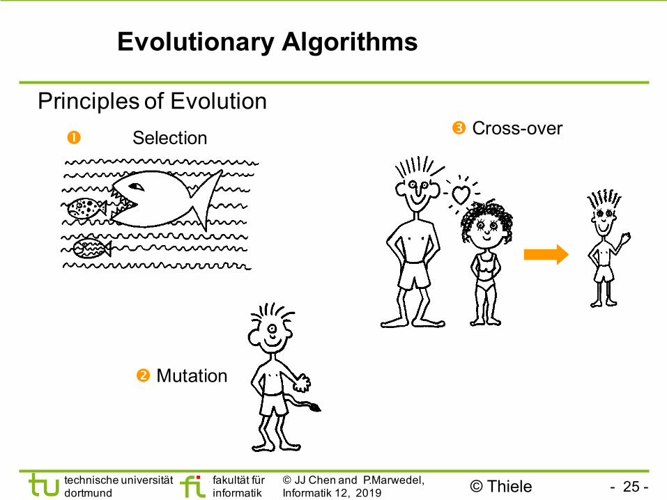
Evolutionary Algorithms
Principles of Evolution Selection Cross-over
Mutation
© Thiele

- 26 -technische universitätdortmund
fakultät für informatik
© JJ Chen and P.Marwedel, Informatik 12, 2019
An Evolutionary Algorithm in Actionmax. y2
min. y1
hypothetical trade-off front
© Thiele

- 27 -technische universitätdortmund
fakultät für informatik
© JJ Chen and P.Marwedel, Informatik 12, 2019

- 28 -technische universitätdortmund
fakultät für informatik
© JJ Chen and P.Marwedel, Informatik 12, 2019
A Generic Multiobjective EA
archivepopulation
new population new archive
evaluatesamplevary
updatetruncate
© Thiele

- 29 -technische universitätdortmund
fakultät für informatik
© JJ Chen and P.Marwedel, Informatik 12, 2019

- 30 -technische universitätdortmund
fakultät für informatik
© JJ Chen and P.Marwedel, Informatik 12, 2019
Simulated Annealing
§ General method for solving combinatorial optimization problems.
§ Based the model of slowly cooling crystal liquids.
§ Some configuration is subject to changes.
§ Special property of Simulated annealing: Changes leading to a poorer configuration (with respect to some cost function) are accepted with a certain probability.
§ This probability is controlled by a temperature parameter: the probability is smaller for smaller temperatures.

- 31 -technische universitätdortmund
fakultät für informatik
© JJ Chen and P.Marwedel, Informatik 12, 2019
Simulated Annealing Algorithm
procedure SimulatedAnnealing;;var i, T: integer;;begini := 0;; T := MaxT;;configuration:= <some initial configuration>;;while not terminate(i, T) dobeginwhile InnerLoop dobegin NewConfig := variation(configuration);;delta := evaluation(NewConfig,configuration);;if delta < 0 then configuration := NewConfig;;else if SmallEnough(delta, T, random(0,1))then configuration := Newconfiguration;;
end;;T:= NewT(i,T);; i:=i+1;;end;; end;;

- 32 -technische universitätdortmund
fakultät für informatik
© JJ Chen and P.Marwedel, Informatik 12, 2019
Explanation
§ Initially, some random initial configuration is created.§ Current temperature is set to a large value.§ Outer loop:• Temperature is reduced for each iteration• Terminated if (temperature ≤ lower limit) or(number of iterations ≥ upper limit).
§ Inner loop: For each iteration:• New configuration generated from current configuration• Accepted if (new cost ≤ cost of current configuration)• Accepted with temperature-dependent probability if(cost of new config. > cost of current configuration).
- 33 -technische universitätdortmund
fakultät für informatik
© JJ Chen and P.Marwedel, Informatik 12, 2019
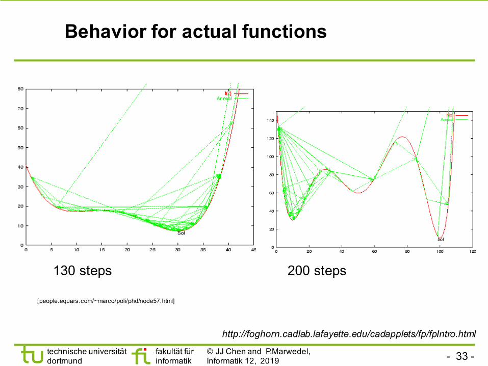
Behavior for actual functions
130 steps
[people.equars.com/~marco/poli/phd/node57.html]
200 steps
http://foghorn.cadlab.lafayette.edu/cadapplets/fp/fpIntro.html
- 34 -technische universitätdortmund
fakultät für informatik
© JJ Chen and P.Marwedel, Informatik 12, 2019
Performance
§ This class of algorithms has been shown to outperform others in certain cases [Wegener, 2005].
§ Demonstrated its excellent results in the TimberWolf layout generation package [Sechen]
§ Many other applications …

- 35 -technische universitätdortmund
fakultät für informatik
© JJ Chen and P.Marwedel, Informatik 12, 2019
Summary
Integer (linear) programming§ Integer programming is NP-complete§ Linear programming is faster§ Good starting point even if solutions are generated with different techniques
Simulated annealing§ Modeled after cooling of liquids§ Overcomes local minimaEvolutionary algorithms§ Maintain set of solutions§ Include selection, mutation and recombination