Evaluation for Transmission Loss Based on Share … Proportion Principle and Sensitivity Analysis...

Evaluation for Transmission Loss Based on

Share Proportion Principle and Sensitivity Analysis

RUI LI

Tokyo Metropolitan University, Minami-Osawa 1-1 Hachioji,

Tokyo 192-0397 Japan

LUONAN CHEN Osaka Sangyo University, Nakagaito 3-1-1, Daito, Osaka 574-8530, Japan

RYUICHI YOKOYAMA Tokyo Metropolitan University,

Minami-Osawa 1-1 Hachioji, Tokyo 192-0397 Japan

Abstract: - This paper presents a method to evaluate the economic value of transmission loss based on the share proportion principle and the sensitivity analysis. We first formulate an optimal power flow problem to derive the operation conditions, the nodal prices of each bus and the transmission prices between two buses, and then trace the transmission loss during operation based on the share proportion principle of the graph theory. The sensitivity analysis has been used to analyze the wheeling path from each generator to any load, and the value of transmission loss is also evaluated. The proposed method is applied to the IEEE 30-bus standard system, which confirms our theoretical results. The proposed method can be used not only to improve the efficient usage of the power grid and congestion management, but also to provide valuable economic signals for the generation or transmission investment. Key-Words: - Transmission loss, Optimal power flow, Share proportion principle, Sensitivity analysis,

Wheeling path 1 Introduction The transmission system is open to access by all power market participants. In an electricity market, it is desirable to account the value of transmissions in a simple, unambiguous and transparent way for all market participants. To keep the system operation impartially, pricing for the cost of transmission losses has become important increasingly in the interest of fair competition with the deregulation of power systems. Despite significant amounts of effort from academic circles and industry, the problem of pricing becomes increasingly complicated due to the rapid advance of deregulation in the power industry. The complexity is caused not only by its internal nonlinearity, but also by the characteristics of market structures and related economic policies [1].

In system operation, the generators and consumers measure their real-time outputs and consumptions, respectively. It is obvious that the generators’ productions should be the sum of load consumptions and transmission loss. Hence, someone in the power market has to pay for the loss. A fair and adequate method for pricing the cost of transmission loss may help the market participants makes appropriate and efficient decisions for power trade.

This paper aims to propose an algorithm to

evaluate the equivalent value of the transmission loss, by applying a decomposition technique for transmission prices [3]. An operation problem of an electric power system as an optimal power flow (OPF) problem is defined firstly. Then the allocation of transmission losses in an open system operating under both pool and bilateral contracts is analyzed. According to the operation solutions, the transmission losses are traced based on the share proportion principle of the graph theory, and such decomposition is unique and continuously. This approach allows considering loss supply as a marketable product, since each bilateral contract can choose its more appropriate loss supplier. Many methodologies which determine the wheeling path have been developed so far, such as the postage stamp methodology and the contract path methodology [1, 8]. However, since in the aforementioned methods, the use of transmission lines and time varying load flows are not reflected sufficiently, shrewd improvements against these problems are desired for the practical use of the methods. In this paper, the extended sensitivity analysis is proposed to identify the wheeling path so that it is possible to fix the proper and fair wheeling rate according to the degree of responsibility of each power flow. Finally, the value of the transmission losses can be derived based on the above calculation

Proc. of the 5th WSEAS/IASME Int. Conf. on Electric Power Systems, High Voltages, Electric Machines, Tenerife, Spain, December 16-18, 2005 (pp398-405)

of OPF and decomposition of wheeling path. In Section 2, an operation problem is formulated

as a nonlinear optimization problem, which has the same form as the conventional OPF. A general explanation is described by deriving the nodal price of each bus and transmission price between any two buses from OPF based-model. Section 3 proposes a theoretical method to determine the amount of transmission loss distributed to each load and to show the contribution of generators to the transmission loss based on the share proportion principle of graph theory. In Section 4 the transmission path is identified by extended sensitivity analysis. The economic value of transmission loss is evaluated. Section 5 is a numerical simulation for IEEE 30-bus system.

2 An Operation Problem Formulation For a n buses system with m generators, let

),,( 1 nPPP K= and ),,( 1 nQQQ K= , where iP and

iQ represent real and reactive power demands of the bus- i respectively. Define voltage variables in the power system operation to be

),,,,( 11 nnVVX θθ K= , which are magnitudes and phases of each bus voltage. ),,( 1 GmGG PPP K= and

),,( 1 GmGG QQQ K= represent the generators outputs, which can be regarded as the functions of

QPX ,, . Therefore, the operation problem of a power

system for the given loads ),( QP can be formulated as the following optimization problem [2],

Min ),,,,( QPQPXf GG for GG QPX ,, (1) s.t. 0),,,,( =QPQPXG GG (2) 0),,,,( ≤QPQPXH GG (3)

where f is a scalar that represents the operating

cost, and can be expressed as ∑==

m

iiff

1 where if is

the operation cost of the i -th generator. T

GGnGG QPQPXgQPQPXgG )),,,,(,),,,,,(( 11 K=

and TGGnGG QPQPXhQPQPXhH )),,,,(,),,,,,(( 21 K=

have 1n and 2n equations respectively, and are column vectors. G is a vector, equality constraints, such as energy balance for generators and loads. H is a vector too, inequality constraints, which includes all variable limits and function limits, such as upper and lower bounds of transmission lines, generation outputs, etc.

Obviously the formulation given by (1)-(3) is a typical OPF problem as far as the demands ),( QP are given. There are many efficient approaches, which can be used to obtain an optimal solution, such as successive linear programming, successive quadratic programming and the Newton method.

From the viewpoint of economics, for a set of given demand ),( QP , the nodal prices of real power for bus-i are expressed below for ni ,,1K= ,

iiii P

HPG

Pf

∂∂

+∂∂

+∂∂

= ρλπ (4)

Therefore, the transmission price of real power is defined as follow,

jiji πππ −=− (5)

where iπ is nodal price of real power at the bus- i ,

ji−π is transmission price of real power at transmission line ji − . ),,( 11 nλλλ K= and

),,( 21 nρρρ K= are the dual variables, and are usually explained as shadow prices. Notice

that ∑ ⋅=⋅=

1

1),,,,(),,,,(

n

iGGiiGG QPQPXgQPQPXG λλ

and ∑ ⋅=⋅=

2

1),,,,(),,,,(

n

iGGiiGG QPQPXhQPQPXH ρρ .

The above formulation is conventional OPF, and the results are fundamental for the evaluation for transmission loss in real-time operation, such as, output of each generator GiP , power flow of each transmission line ijP , nodal prices iπ and transmission price ijπ . 3 The Amount of Transmission Loss In real-time operation, consumers measure their actual consumption, while generator meters measure their actual productions. The transmission loss is the difference between generator outputs and load consumptions. If there is not any transmission loss, more power should be conveyed from generators to the loads than realistic operation. The gross power supplied to each load is symbolized as

),,( 1 dndd PPP K= , which is the sum of real power demand and transmission loss ),,( 1 snss PPP K= distributed to each load, i.e.,

)(111

sin

ii

n

idi

m

iGi PPPP ∑ +=∑=∑

=== (6)

Next, we establish the matrix of power flow which is symmetrical with half positive and half


negative values based on OPF calculation. For any bus, the transmission lines can be divided into two groups, injecting lines and emitting lines. In this section, in

iα and outiα represent the two aggregates

which inject into and flow out from bus-i, respectively. 3.1 Share Proportion Principle From the viewpoint of graph theory, the power network is kind of graph with direction, while the buses and transmission lines are nodes and branches, respectively. The share proportion principle can be used to analyses power flow at each bus.

Fig. 1 shows an example without any loss for the share proportion principle. Node-i connects with 3 injecting branches and 2 emitting branches, i.e.,

{ }CBAini ,,=α and { }FEout

i ,=α .Without any loss, 1004060503020 =+=++ , i.e., the 3 branches

supply the power to node-i by 20%, 30% and 50%, respectively. It is reasonable to hypothesize that each emitting branch shares same proportion as the node connected with. For instance, for branch-E, 20% comes from branch-A, left 30% and 50% come from branch-B and C. In the other word, the injected power is mixed at nod-i, and sent out as the same rate to any emitting branches.

50

20

30

60

40

A

B

C

E

F

i

Fig. 1 An example without any loss for the share

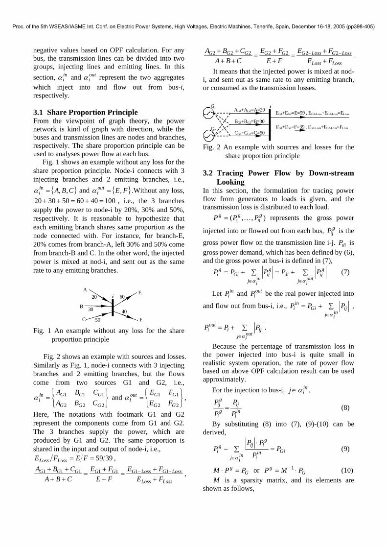
proportion principle Fig. 2 shows an example with sources and losses.

Similarly as Fig. 1, node-i connects with 3 injecting branches and 2 emitting branches, but the flows come from two sources G1 and G2, i.e.,

⎭⎬⎫

⎩⎨⎧

=222

111

GGG

GGGini CBA

CBAα and

⎭⎬⎫

⎩⎨⎧

=22

11

GG

GGouti FE

FEα ,

Here, The notations with footmark G1 and G2 represent the components come from G1 and G2. The 3 branches supply the power, which are produced by G1 and G2. The same proportion is shared in the input and output of node-i, i.e.,

3959== FEFE LossLoss ,

LossLoss

LossGLossGGGGGGFEFE

FEFE

CBACBA

++

=++

=++++ −− 1111111 ,

LossLoss

LossGLossGGGGGGFEFE

FEFE

CBACBA

++

=++

=++++ −− 2222222 .

It means that the injected power is mixed at nod-i, and sent out as same rate to any emitting branch, or consumed as the transmission losses.

EG1+EG2=E=59 , EG1-Loss+EG2-Loss=ELoss AG1+AG2=A=20 i

CG1+CG2=C=50

G1

BG1+BG2=B=30G2

FG1+FG2=F=39 , FG1-Loss+FG2-Loss=FLoss

Fig. 2 An example with sources and losses for the

share proportion principle 3.2 Tracing Power Flow by Down-stream

Looking In this section, the formulation for tracing power flow from generators to loads is given, and the transmission loss is distributed to each load.

),,( 1g

ngg PPP K= represents the gross power

injected into or flowed out from each bus, gijP is the

gross power flow on the transmission line i-j. diP is gross power demand, which has been defined by (6), and the gross power at bus-i is defined in (7),

∑+=∑+=∈∈ out

ij

gijdi

inij

gijGi

gi PPPPP

αα (7)

Let iniP and out

iP be the real power injected into

and flow out from bus-i, i.e., ∑+=∈ in

ijijGi

ini PPP

α ,

∑+=∈ out

ijiji

outi PPP

α.

Because the percentage of transmission loss in the power injected into bus-i is quite small in realistic system operation, the rate of power flow based on above OPF calculation result can be used approximately.

For the injection to bus-i, inij α∈ ,

ini

ijg

i

gij

P

P

P

P= (8)

By substituting (8) into (7), (9)-(10) can be derived,

∑ =⋅

−∈ in

ijGiin

i

giijg

i PP

PPP

α (9)

Gg PPM =⋅ or G

g PMP ⋅= −1 (10) M is a sparsity matrix, and its elements are

shown as follows,


[ ]⎪⎪⎩

⎪⎪⎨

⎧

∈−

=

=

others

jP

Pji

M iniin

i

ijij

0

1

α

For the flow out bus-i, outij α∈ ,

outi

ijg

i

gij

P

P

P

P= (11)

By substituting (11) into (7), (12)-(13) can be derived,

∑⋅

−=∈ out

ijout

i

giijg

idi P

PPPP

α (12)

gd PNP ⋅= (13)

N is also a sparsity matrix, and its elements are shown as follow,

[ ]⎪⎪⎩

⎪⎪⎨

⎧

∈−

=

=

others

jP

Pji

N outiout

i

ijij

0

1

α

According to (6), (10) and (13), the transmission loss sP distributed to each load can be obtained by (14),

PPMNP Gs −⋅⋅= −1 (14) (14) seems to have given a full description for

tracing transmission loss even without any further analysis. However it is still unknown exactly which generator supplies, how much power is supplied for the transmission loss and what kind of wheeling path the lost power is passed. 3.3 Decomposition for Transmission Losses To decompose the components of transmission loss, the share proportion principle is used again to trace the power flow from each generator side to any load side.

Start from the bus connected with a generator but without any injection line, it is obvious that the power flows which flow out from this bus are provided hundred percent by this generator. And all transmission lines keep the rates provided by generators. Let GksiP − and GkijP − be the contributions of generator-k for transmission loss

siP and for the power flow which is burdened by line-ij, respectively.

For bus-i, the proportion of composition for transmission loss can be shown as (15), ni ,,1K= ,

),,1( mk L∈ ,

ini

inij

GkijGk

si

Gksi

P

PP

PP

∑+

=∈

−

− α (15)

If ik = , the generator injects all production to bus-i. When ik ≠ , GkP should be zero in (15). The procedure for tracing transmission loss can be described in Fig 3.

Scan from i=1,n

Yes K=1,m

All injection line with the proportion of production from each generator

Derive the proportion for transmission loss by (15)

Output

No

Start

End Fig. 3 Flowchart of decomposition for the

transmission losses

4 Evaluation for Transmission loss

based on Sensitivity Analysis In this section, the sensitivity analysis is derived to distribute the wheeling path for the transmission loss in the grid theoretically. Firstly, the sensitivity method in power system is formulated. Then, a practical and efficient method is proposed to identify the wheeling paths of transmission loss from each generator to any customers. Finally, the transmission loss is evaluated based on sensitivity analysis results. 4.1 Sensitivity Analysis in Power System Let the voltage vector iV at node-i be expressed in polar form and the admittance ijijij jBRY += in rectangular form. Then power flow equation is a set of 2n real simultaneous equations, for ni ,,2,1 L= ,

( ) ( )[ ] 0sincos1

12 =∑ −+−+−==

−n

jjiijjiijjiGiii BRVVPPG θθθθ

( ) ( )[ ] 0cossin1

2 =∑ −−−+−==

n

jjiijjiijjiGiii BRVVQQG θθθθ

For simplicity, the variables and parameters involved in above power flow equations will be classified into two vectors. They are dependent variable vector Z wit t dimensions and


controllable variable vector U with k dimensions comprising the operating variables in system analysis and control.

Using two vectors UZ , defined above, the power flow is expressed by the following simple equation vector,

( ) 　0, =UZG (16) where G is a 2n-dimensional column vector

function. The pair of vectors 0Z and 0U satisfies (16), i.e., ( ) 　0, 00 =UZG .

Assume that by changing the operating condition of regulating devices, the controllable variable vector U has experienced a change U∆ from 0U . If dependent variable vector Z changes from 0Z to

ZZ ∆+0 in accordance with the change U∆ , then there is ( ) 0, 00 =∆+∆+ UUZZG .

If U∆ is very small, then the variance Z∆ is generally small. By applying Taylor's series expansion with ( )00 ,UZ as the reference state and neglecting higher order terms in Z∆ and U∆ , we have

0),(),(),( 000000 =∆+∆+ UUZGZUZGUZG UZ (17) where ZGGZ ∂∂= , UGGU ∂∂= are the

Jacobian matrix of G with respect to the dependent variable vector UZ , . Since the first term of (17) is eliminated,

UGGZ UZ ∆⋅⋅−=∆ −1 (18)

Let UZ GGS ⋅−≡ −1 , (18) can be rewritten in the form of (19),

USZ ∆⋅=∆ (19) or more concretely in following form,

　

⎟⎟⎟⎟⎟

⎠

⎞

⎜⎜⎜⎜⎜

⎝

⎛

∆

∆∆

⎟⎟⎟⎟⎟

⎠

⎞

⎜⎜⎜⎜⎜

⎝

⎛

=

⎟⎟⎟⎟⎟

⎠

⎞

⎜⎜⎜⎜⎜

⎝

⎛

∆

∆∆

ktktt

k

k

t u

uu

SSS

SSSSSS

z

zz

M

L

LLLL

L

L

M2

1

21

22221

11211

2

1

The kt × coefficient matrix S in (19) is called the sensitivity matrix of power flow with respect to the controllable variable vector U . 4.2 Identifying Wheeling Paths of

Transmission loss We derive the sensitivity constants which are required for power flows of each transmission line for identifying the wheeling paths.

For a system with n buses, m generators and l transmission lines, let F be the power current. By the use of the two vectors X and P , the line flows are conveniently expressed by the simple function

vector ( )PXF , , where F is an l -dimensional column vector function.

Let us assume that when the state of the system is changed from an initial state ( )00 , PX to a state ( )PPXX ∆+∆+ 00 , by the operation of some regulating devices, line flows are also changed by

( )00 , PXF∆ . Similar to (17), the Taylor series expansion with ( )00 , PX as the reference state yields,

( ) ( ) ( ) PPXFXPXFPXF PX ∆+∆=∆ 000000 ,,, (20) Let FS be the sensitivity matrix representing the

change in power flow F∆ due to a change P∆ in transmission loss. In this paper, sP is regarded as the change of load demand P∆ , i.e., sF PFS ∆= . Partial derivatives, XFFX ∂∂= and PFFP ∂∂= are obtained quite easily by simple calculation

PX ∂∂ / which is already known as the elements of the sensitivity matrix (19).

From (20), the following relation is obtained. ( ) ( ) ( )0000

00 ,,, PXFPXPXF

PPXFS PX

sF +

∂∂⋅=

∆= (21)

Let ijF be the power flow on the transmission line ji − . Generally, (21) can be used to calculate the line currency.

[ ]ijijij

jiji

ijijij

jijijiiij BBR

VV

RBR

VVVVVF

)(

)sin(

)(

2)(sin2)(2222

2

+

−+

+

−⋅+−⋅=

θθθθ (22)

Then the related wheeling path of transmission loss is identified by examining the magnitude of sensitivity factors from generator to load. 4.3 Evaluation for Transmission Loss Based on the above analysis results, the economic value of transmission loss can be evaluated easily. We separate the values into two parts; one is for power production, and the other is for power transmission. Here it is assumed that power consumers pay for the transmission loss, which also can be shared by other power market participators, or be regarded as a kind of service provided by utility.

For a n -bus system with m generators and l transmission lines, i) Pricing of power production for transmission loss:

The payment of bus-i: ∑ ⋅=

−m

jjgjsiP

1)( π

The income of generator-j: ∑⋅=

−n

igjsij P

1π

ii) Pricing of power transmission for transmission loss: There two conditions have to be considered.


(a) All lines belong to one grid company.

The payment of bus-i: ∑ ⋅=

−m

jijgjsiP

1)( π

The income of the grid company:

∑ ∑ ⋅= =

−n

i

m

jijgjsiP

1 1)( π

(b) The lines belong to plural grid companies. If the loads and generators belong to different

companies, the wheeling paths have to be traced to derive the amount of power flow through the boundary bus or buses. For example, there are two grid companies in a system. Company A holds a part of lines and all generators, and B is the owner of the rest lines and all loads. t

gjsiP − and rgjsiP −

represent the transmission losses pass bus- t and bus- r which are boundary of two companies,

),,1(, nrt K∈ . Note that rgjsi

tgjsigjsi PPP −−− += .

The bus-i for company A:

∑ ⋅+∑ ⋅=

−=

−m

jjr

rgjsi

m

jjt

tgjsi PP

11)()( ππ

The bus-i for company B:

∑⋅+∑=

−=

−m

j

rgjsiir

m

j

tgjsiit PP

11ππ

5 Case Study 5.1 System Description The IEEE 30-bus system is used to illustrate the proposed methodology. As shown in Fig. 7 or Fig. 8, the system has 30 buses, 19 loads and 41 transmission lines.

In this paper, as same as the power demand of each bus QP, , all limits are regarded as given conditions. It is assumed that the voltage value for all buses is bounded between 0.95 and 1.05; the power flow in each line is restricted between -0.7 and 0.7. All the values are indicated by p.u. 5.2 Numerical Simulation The load demands are the given conditions. The generator outputs are presented based on OPF calculation results, and the allocated transmission loss to either generators or loads is shown in Tables 1 and 2. The generator outputs are 238.516MW, in which 6.816MW is used by transmission loss.

In Table 2, if there were not transmission loss in system operation, more power should be transported to the loads. The gross power at each load is the sum of real demand and loss distributed on that bus, i.e., the gross power of bus-3 is KWMW 7.304.2 + . “%”

indicates the percentage of loss in load demand. Due to less than 5%, they are small enough to fit for sensitivity analysis. Table 2 also shows the allocation by tracing the source of transmission loss, i.e., the transmission loss of bus-10 is 87.65KW, in which 4.98KW is supplied by generator G1, 3.7KW, 74.78KW and 4.19KW are supplied by generator G2, G22 and G27, respectively. It is clear that G22 provides much more than other generators, because G22 is much closer to bus-10 than the others.

Table 1. Results of Generator Output (MW) Total output For load demand For loss

G1 73.67 71.3714 2.2986G2 61.656 59.5277 2.1283

G22 53.19 52.2303 0.9597G27 50 48.5705 1.4295Total 238.516 231.7 6.8160

Table 2. Distribution of the Transmission Loss

Bus No.

Load demand

MW

Loss on each load

KW

From G1 KW

From G2 KW

From G22 KW

From G27KW %

3 2.4 30.70 30.70 0 0 0 1.284 7.6 116.97 89.00 27.97 0 0 1.545 94.2 3520.46 1433.87 1693.27 0 393.32 3.747 22.8 942.68 364.49 271.03 0 307.17 4.14

10 5.8 87.65 4.98 3.70 74.78 4.19 1.5112 11.2 235.92 162.02 51.52 21.19 1.19 2.1114 6.2 150.31 87.61 27.86 18.95 15.88 2.4215 8.2 273.24 79.19 25.18 62.40 106.46 3.3316 3.5 76.84 4.36 3.24 65.56 3.68 2.2017 9 197.60 11.22 8.34 168.58 9.46 2.1918 3.2 96.51 18.71 6.91 46.88 24.02 3.0219 9.5 185.41 10.53 7.83 158.18 8.87 1.9520 2.2 33.25 1.89 1.40 28.36 1.59 1.5121 17.5 172.39 0 0 172.39 0 0.9923 3.2 131.39 0 0 43.30 88.09 4.1124 8.7 300.86 0 0 99.15 201.71 3.4626 3.5 85.94 0 0 0 85.94 2.4629 2.4 40.09 0 0 0 40.09 1.6730 10.6 137.81 0 0 0 137.81 1.30

Total 231.7 6816 2298.56 2128.27 959.71 1429.47 2.94

0%

20%

40%

60%

80%

100%

1 2 3 4 5 6 7 8 9 10 11 12 13 14 15 16 17 18 19 20 21 22 23 24 25 26 27 28 29 30Bus

G1 G2 G22 G27 Fig.4. Percentage of transmission loss from

generators to loads Fig. 4 represents the percentage of transmission

loss from generators to each load. In a grid network without special contract, the generators provide the power to closer load priority. The transmission loss takes place during the transportation of power demand. The closer generator takes the more transmission loss for any load, for example, G1


burdens all transmission loss for load-3, and G27 burdens all transmission loss for load-27, 29 and 30.

The payment is divided into two parts; one is for generator output, and the other is for wheeling service. We have assumed that the power consumers pay for the transmission loss. Because the generator and load use the grid at the same time, both of them should share the payment, which can be determined by negotiations.

Fig.5 presents the payment of transmission loss for generator outputs. The total payment of generator output for transmission loss is $375.7, which is shared by G1 $128.73, G2 $121.82, G22 $48.64 and G27 $76.5. The load-5 and load-7 have to pay much more than others, owing to their large amount of power demand and long electric distances.

If all transmission lines belong to a single grid company, there is not necessary to identify the wheeling paths for transmission loss, because the congestion has been generally alleviated by OPF calculation, and the transmission price is determined by the difference between two nodal prices of the buses connected with generator and load.

Fig.5. Payment of transmission loss for generators

output by loads

Fig.6. Payment of transmission loss for wheeling by

loads

C

C

2G1

G2

G22

G27

5 7 8

28

27

2930

25

26

24 23

22

10

6

9 11

17 16

12

14

15

4 3

13

18 19 20 21

1

25.18KW 79.19KW

62.4KW

106.46KW

$0.4915 $0.1396

$0.4237

$0.1715$1.2263273.24KW

Fig.7. Wheeling path and amount of transmission

loss to bus-15

C

C

2G1 G2

G22

G27

5 7 8

Line 2-5 Line 5-7

28

27

2930

25

26

24 23

22

10

6

9 11

17 16

12 14

15

4 3

13

18 19 20

21

1

1693.27KW 1433.87KW

3520.46KW

393.32KW

Fig.8. Wheeling path and amount of transmission

loss to bus-5 Fig. 6 shows the payment of transmission loss for

wheeling. The total payment of wheeling for transmission loss is $59.215, which is no difference, when there is only one or plural owners of transmission lines in this 30-bus system. As shown in Fig. 7, the load-15 has to pay $1.2263 for transportation of the loss from four generators, G1 $0.4915, G2 $0.1396, G22 $0.1715 and G27 $0.4237, respectively. The transmission route is shown in Fig. 7.

Next it is assumed that there are two line-owners in the target system, i.e., grid company A and B. Company B holds the lines 2-5 and 5-7, and the other lines all belong to company A. In other words, the boundary of two companies is bus-2 and bus-7. According to OPF result, load-5 is the only user of lines 2-5 and 5-7, which has to pay for both


companies A and B. Fig.8 shows the wheeling path and mount of transmission loss to bus-5, where only 3 generators’ productions are effected by transmission loss to load-5.

G1 kwe /$344.1252 −=−π

kwe /$463.621 −=−π

kwe /$355.971 −=−π

kwe /$306.772 −=−π

kwe /$304.7727 −=−π

G1

G2

G27

G2

kwe /$335.457 −=−π

638.82kw

890.61kw 1529.43kw

1991.03kw

795.09kw

802.62kw

392.32kw

Bus-7

Bus-2

Bus-5

Company A Company B

Fig.9. Illustration of Distribution transmission loss

to bus-5

$19.03, 43.11%

$8.66, 19.62%

$0.424 0.96%

$5.667 12.84%

$2.769 6.27%

$16.451 37.27% $7.591

17.20%

on line 2-5 on line 5-7 G1 to Bus 2 G1 to Bus 7 G2 to Bus 7 G27 to Bus 7

Company B Company A

Fig.10. Payment of load-5 to company A and B for

transmission loss

The total payment of load-5 for transmission loss is $44.14. How to share this payment depends on the wheeling paths for transmission loss. Figs. 9 and 10 illustrate how two companies share the payment. As shown in Fig. 9, the company A carries power from G1 638.82KW to bus-2, and total 1991.03KW from G1, G22 and G27 to bus-7, while the company B transport the loss power to bus-5 contiguously. The G2 output for this transmission loss is 1693.27KW, in which 890.61KW is injected into company B area directly, and 802.62KW is injected into company B area after they are transported to bus-7 by company A. In the area of company A, 392.32KW is transported from G27 to bus-7 by lines 27-28, 28-6, 28-8, and 8-6, which have the transmission price 304.7727 −=− eπ $/KW. The charge for this transportation is $2.769, 6.27% in total payment of load-5 for transmission loss. For company B, 1529.43KW and 1991.03KW are transported by lines 2-5 and 7-5, which have the

wheeling prices 344.1252 −=− eπ $/KW and 335.457 −=− eπ $/KW. The payment of load-5 for

transmission loss is shared by company A $16.45 and company B $27.69. The payment for loss is decided by the electric distance and the amount of power. 6 Conclusion A pricing technique has been proposed to evaluate the equivalent values of the transmission loss by the sensitivity analysis and the share proportion principle. It has shown that transmission loss can theoretically be evaluated, or traced from the viewpoint of economics. To verify the effectiveness of the proposed method, the simulations have been conducted on the IEEE 30-bus test system, which confirms the effectiveness of the proposed method. The theoretical results enable us to evaluate the values of transmission losses for market players in the power system easily and effectively. As the future studies for implementation of the proposed approach, the time varying demand, the adaptation of the transaction framework to reactive power and voltage and the volatility of electricity prices in power markets should be taken into consideration. References: [1] R. Yokoyama, "Liberalization of Electricity Markets

and Technological Issues", Tokyo Denki University Press, 2001.

[2] C. C. Kelley, “Iterative Method for Optimization”, Frontiers in Applied Mathematics, 1999.

[3] L.Chen, H.Suzuki, T.Wachi and Y.Shimura, "Components of Nodal Prices for Electric Power Systems", IEEE Trans. on Power Systems, Vol. 17, No. l, pp. 41-49, 2002.

[4] M. C. Caramanis, R. E. Bohn and F. C. Schweppe, "Optimal Spot Pricing: Theory and Practice," IEEE Transactions on Power Apparatus and Systems, Vol. 101, No. 9, September 1982

[5] Asano H, Okada K. "Development of Computation Method for Regional Electric Transmission Capacity Pricing," Transactions IEE Japan, Vol. 117, 61-7, 1997

[6] Shu Tao and George Gross, "Transmission Loss Compensation in Multiple Transaction Networks," IEEE Trans. on Power Systems, Vol. 15, No. 3, 909-915, 2000

[7] A. J. Conejo, J. M. Arroyo, and N. Alguacil, "Transmission Loss Allocation: A Comparison of Different Practical Algorithms," IEEE Trans. on Power Systems, Vol. 17, No. 3, 571-576, 2002

[8] Phichaisawat S, Song YH, "Transmission Pricing Using Improved Sensitivity Indices," IEEE Power Engineering Society Winter Meeting 2001;3:1250-5.


Evaluation for Transmission Loss Based on Share … Proportion Principle and Sensitivity Analysis...

Documents

Transcript of Evaluation for Transmission Loss Based on Share … Proportion Principle and Sensitivity Analysis...