中国家庭汽车拥有水平影响因子的非集计分析 · Taiwan, as well as Xinjiang, Tibet,...

http://www.sinoss.net

- 1 -

中国家庭汽车拥有水平影响因子的非集计分析

邵长凯

（湖南大学经济管理研究中心，湖南省长沙市，410006）

摘要：过去三十年间，伴随着高速的经济发展和快速的城市化进程，中国的私家车保有量经历了爆炸性的

增长。同时，由于汽车和家庭居住地点、出行方式、出行里程、交通政策等要素有着密切的联系，私家车

在家庭生活中往往扮演着重要的角色。鉴于此，能够准确且全面的理解家庭汽车拥有行为便显得至关重要。

本文中，以《中国家庭追踪调查》数据为样本，我们运用多元响应 logit 模型和有序 logit 模型在家庭微

观层面上研究中国家庭汽车拥有水平的潜在影响因子。本研究中，家庭汽车拥有水平被划分为 0，1,和 1+

三个类别。通过将家庭金融要素分解为家庭收入因子和家庭净资产因子，我们构建了两组相应的分类变量。

此外，影响因子还包括家庭结构类分类变量和其他变量。通过运用最大似然估计法，我们得到了一系列的

一致、有效、且渐进正态分布的估计量。估计结果分析表明通过纳入家庭净资产要素，我们能够得到更准

确的预测。其中，家庭收入的效用相对未囊括净资产要素模型估计的效用要小。进入婚姻状态对家庭第一

辆汽车购买起着积极的作用，这可能源于家庭收入来源和出行需求的增加。家庭金融要素和家庭结构要素

作为汽车购买和需求的根源，在家庭汽车拥有行为中起着主要的作用。城乡二元体系在家庭汽车拥有行为

中不再产生作用。预测分析表明现在以及未来一段时间，中国的汽车市场拥有着巨大潜力，但同时一辆汽

车依然是大多数中国家庭汽车拥有水平的上限。拟合优度表明多元响应 logit 模型和有序 logit 模型在样

本数据拟合表现上差异不大。此外，通过构建汽车拥有水平特征变量，家庭交通支出，运用本多元响应 logit

模型和条件 logit 模型的混合模型，研究提供了一个理解中国家庭汽车拥有行为的更好的方法。在现实应

用中，本研究发现可以帮助政策制定者有效控制私家车增长带来的负面效用，同时，也能够帮助汽车生产

厂商制定更加合理的生产计划。本研究也有一些不足之处，一方面体现在所用 2010年数据有些过时，另一

方面体现在缺少影响家庭汽车拥有行为的城市结构变量。

关键词：家庭汽车拥有水平；非集计分析；金融要素分解；家庭净资产；

中图分类号： F572.88 文献标识码：A

1, Introduction

With tremendous economic growth and fast-paced urbanization in past decades in

China, the amount of private motor vehicles has been going through an explosive growth.

The number of private motor vehicle in 1991 was 960 thousand and increased to 1,459.8

million in 2015, 152 times increased in 25 years and 6 times increased annually at the

national level. And the number of private vehicle per 1000 persons increased from 0.8 in

1991 to 106.73 in 2014(China Statistical Yearbook).

Private motor vehicle ownership has played an important role in a household’s daily life

for which it is fundamentally interconnected with residential location, family travel modes,

vehicle miles traveled and transportation policy analysis (Scott and Axhausen 2006).

Meanwhile, the rising prevalence of private cars in China is causing serious issues,

including traffic congestion, air pollution, and traffic accidents. To reduce these

vehicle-related problems in some cities, local government has undertaken studies such

like laying a high vehicle purchase tax, a license plate number lottery, or other policies

(Hao, Wang et al. 2011).

2, Literature Review

This section will provide a critical overview of previous empirical studies on household

vehicle ownership decision. Two relevant issues are going to be discussed: (I) model


- 2 -

types used in household vehicle ownership analysis, and (II) determinants of individual

household vehicle ownership level.

(I) Model types used in household vehicle ownership analysis

According to level of aggregation and data requirements, model types used in

household vehicle ownership studies can be split into two groups: aggregate models and

disaggregate models. Earlier household vehicle ownership literatures tended to focus on

aggregate analysis of the relationship between vehicles per household or vehicles per

individual and the associated explanatory variables at the national or regional level(De

Jong, Fox et al. 2004). Within these literatures, the most frequently tested influence factor

is the national or regional economic development index, such as per capita income or

regional GDP. The local per capita income was the primary positive determinant on

average household vehicle ownership (Dargay and Gately 1999, Holtzclaw, Clear et al.

2002). Using an aggregate level panel dataset from 26 countries over the period

1960-1992 covering from the lowest to highest income level, Dargay and Gately (1999)

used the Gompertz function to explore the growth of car and vehicle ownership per

individual as a function of per-capita income. By estimating the long and short run income

elasticity, they found that compared with developed countries, there existed a stronger

historical relationship between the growth of per-capita income and the growth of average

car and vehicle ownership at national level in low income countries, such as China and

India. To exam the hysteresis or asymmetric problem of the effect of income on car

ownership, based on the cohort pseudo panel data constructed from 1970 to 1995 UK

Household Expenditure Survey, Dargay (2001) introduced a dynamic econometric model

relating the average household car ownership to household income and lagged car

ownership, accompanied with some other correlated explanatory variables. Be estimating

the car ownership elasticities with respect to rising and falling household income, Dargay

found that there was stickiness of car ownership in the falling income direction.

Considering the disadvantages in modeling household vehicle ownership for aggregate

approach, researchers have made use of the disaggregate models which incorporated

individual household’s and members’ information in recent years. Compared with

aggregate models, disaggregate models are structurally more behavioral and better able

to capture the causal relationship between individual household vehicle ownership and its

influential factors (Bhat and Pulugurta 1998).

(II) Determinants of individual household vehicle ownership level

By using aggregate and disaggregate models to investigate household vehicle

ownership, researchers have found out various influencing factors based on available

survey data and previous empirical studies. Influential factors can be categorized into

several groups, including household social-economic factors, as well as household

demographic characteristics, residential location and other variables.

Based on a review of relevant literatures which incorporate both aggregate and

disaggregate studies, a clear and common indication is that household economic level is

the primary determinant of vehicle ownership. One of the common economic level indexes

in household income. The empirical evidence demonstrates that vehicle ownership is a

strong normal good with demand elasticity that is typically greater than 1. And it’s more

elastic in low income countries (Dargay and Gately 1999). The effects of income can be


- 3 -

summarized like this: the higher the household income, the more likelihood a household

owns more vehicles (Bhat and Pulugurta 1998, Dargay and Gately 1999, Chu 2002,

Holtzclaw, Clear et al. 2002, Kim and Kim 2004, Dargay and Hanly 2007, Whelan 2007,

Clark 2009). This is also true for household vehicle ownership decisions in China both

from aggregate and disaggregates perspectives (Riley 2002, Li, Walker et al. 2010, Wang

and Wang 2014, Zhang, Jin et al. 2017). The annual household income is the most

usually introduced in the disaggregate specification (Bhat and Pulugurta 1998, Chu 2002,

Dargay and Hanly 2007, Clark 2009, Zhang, Jin et al. 2017). Kim and Kim (2004) used the

per-capita income within a household calculated by the ratio of total household income

and household size. Nolan (2010) applied the real net household income in the

explanation variables. Wang and Wang (2014) taken the monthly household income in the

specification.

Besides household income, the household size and composition, such like household

life-cycle stages, are thought to play an important role in determining household vehicle

ownership level(Karlaftis and Golias 2002). Prevedouros and Schofer (1993) found that

changes in household life-cycle stages alone could cause household automobile

ownership to increase or decrease substantially. Giuliano and Dargay (2006) built

household life-cycle stage variables in the structural model with daily travel conditional

upon car ownership and a reduced form model for daily travel. Whelan (2007) constructed

8 household categories based on the number of household adults, children(under 17s)

and employment status according to those defined in the UK’s national transport model.

Accompanied with household income, they concluded strong explanation effects of these

variables on household vehicle ownership level. Potoglou and Kanaroglou (2008)

introduced five categories of household type based on household life-cycle stage, namely

(a) single, (b) couple, (c) couple with children, (d) single parent and (e) extended families

or unattached individuals, in their disaggregate model.

In addition, the nature of the area in which the household lives in is another important

influence factor on household vehicle ownership, especially considering the administrative

urban-rural division system in China. Residential location effects are usually correlated

with variables like urban location, rural location, distance to CBD and ring road location.

Based on the degree of urbanization in the residential area, Bhat and Pulugurta (1998)

used two residential location descriptors: urban and rural residential location variables, to

capture attributes of a household's activity-travel environment. (Prevedouros and Schofer

1993) demonstrated that residence location into outer-ring, low-density suburbs

decreased household automobile ownership. However, considering the economic

development level and life style in China, effects of residential location may exhibit

differently. Based on a survey study in Beijing and Chengdu, households tended to

purchase fewer cars when they lived further away from the CBD where amenities were

readily available (Li, Walker et al. 2010). Wang and Wang (2014) also studied the effects

of living in inner-ring area or not in Beijing , and they concluded insignificant effects of

these location variables. At the community-level, the higher neighborhood population

density is believed to have significant negative effects on vehicle ownership level both in

China (Li, Walker et al. 2010) and the US (Schimek 1996).

3, Data sources and descriptive statistics


- 4 -

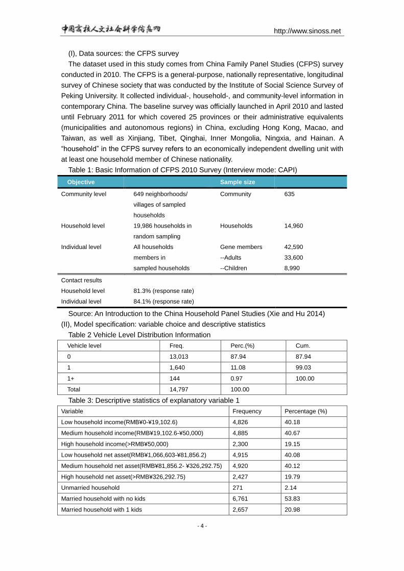
(I), Data sources: the CFPS survey

The dataset used in this study comes from China Family Panel Studies (CFPS) survey

conducted in 2010. The CFPS is a general-purpose, nationally representative, longitudinal

survey of Chinese society that was conducted by the Institute of Social Science Survey of

Peking University. It collected individual-, household-, and community-level information in

contemporary China. The baseline survey was officially launched in April 2010 and lasted

until February 2011 for which covered 25 provinces or their administrative equivalents

(municipalities and autonomous regions) in China, excluding Hong Kong, Macao, and

Taiwan, as well as Xinjiang, Tibet, Qinghai, Inner Mongolia, Ningxia, and Hainan. A

“household” in the CFPS survey refers to an economically independent dwelling unit with

at least one household member of Chinese nationality.

Table 1: Basic Information of CFPS 2010 Survey (Interview mode: CAPI)

Objective Sample size

Community level

649 neighborhoods/

villages of sampled

households

Community 635

Household level 19,986 households in

random sampling

Households 14,960

Individual level All households

members in

sampled households

Gene members

--Adults

--Children

42,590

33,600

8,990

Contact results

Household level

Individual level

81.3% (response rate)

84.1% (response rate)

Source: An Introduction to the China Household Panel Studies (Xie and Hu 2014)

(II), Model specification: variable choice and descriptive statistics

Table 2 Vehicle Level Distribution Information

Vehicle level Freq. Perc.(%) Cum.

0 13,013 87.94 87.94

1 1,640 11.08 99.03

1+ 144 0.97 100.00

Total 14,797 100.00

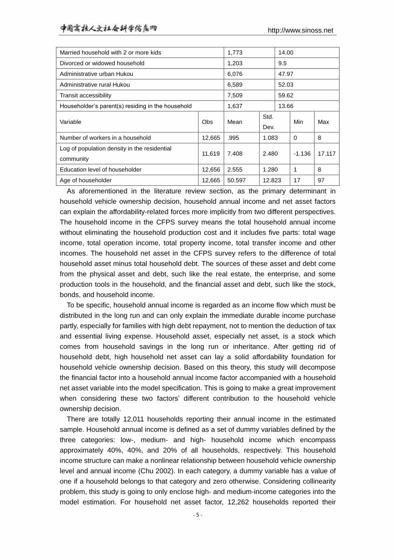
Table 3: Descriptive statistics of explanatory variable 1

Variable Frequency Percentage (%)

Low household income(RMB¥0-¥19,102.6) 4,826 40.18

Medium household income(RMB¥19,102.6-¥50,000) 4,885 40.67

High household income(>RMB¥50,000) 2,300 19.15

Low household net asset(RMB¥1,066,603-¥81,856.2) 4,915 40.08

Medium household net asset(RMB¥81,856.2- ¥326,292.75) 4,920 40.12

High household net asset(>RMB¥326,292.75) 2,427 19.79

Unmarried household 271 2.14

Married household with no kids 6,761 53.83

Married household with 1 kids 2,657 20.98


- 5 -

Married household with 2 or more kids 1,773 14.00

Divorced or widowed household 1,203 9.5

Administrative urban Hukou 6,076 47.97

Administrative rural Hukou 6,589 52.03

Transit accessibility 7,509 59.62

Householder’s parent(s) residing in the household 1,637 13.66

Variable Obs Mean Std.

Dev. Min Max

Number of workers in a household 12,665 .995 1.083 0 8

Log of population density in the residential

community 11,619 7.408 2.480 -1.136 17.117

Education level of householder 12,656 2.555 1.280 1 8

Age of householder 12,665 50.597 12.823 17 97

As aforementioned in the literature review section, as the primary determinant in

household vehicle ownership decision, household annual income and net asset factors

can explain the affordability-related forces more implicitly from two different perspectives.

The household income in the CFPS survey means the total household annual income

without eliminating the household production cost and it includes five parts: total wage

income, total operation income, total property income, total transfer income and other

incomes. The household net asset in the CFPS survey refers to the difference of total

household asset minus total household debt. The sources of these asset and debt come

from the physical asset and debt, such like the real estate, the enterprise, and some

production tools in the household, and the financial asset and debt, such like the stock,

bonds, and household income.

To be specific, household annual income is regarded as an income flow which must be

distributed in the long run and can only explain the immediate durable income purchase

partly, especially for families with high debt repayment, not to mention the deduction of tax

and essential living expense. Household asset, especially net asset, is a stock which

comes from household savings in the long run or inheritance. After getting rid of

household debt, high household net asset can lay a solid affordability foundation for

household vehicle ownership decision. Based on this theory, this study will decompose

the financial factor into a household annual income factor accompanied with a household

net asset variable into the model specification. This is going to make a great improvement

when considering these two factors’ different contribution to the household vehicle

ownership decision.

There are totally 12,011 households reporting their annual income in the estimated

sample. Household annual income is defined as a set of dummy variables defined by the

three categories: low-, medium- and high- household income which encompass

approximately 40%, 40%, and 20% of all households, respectively. This household

income structure can make a nonlinear relationship between household vehicle ownership

level and annual income (Chu 2002). In each category, a dummy variable has a value of

one if a household belongs to that category and zero otherwise. Considering collinearity

problem, this study is going to only enclose high- and medium-income categories into the

model estimation. For household net asset factor, 12,262 households reported their


- 6 -

household asset situation. Similarly, to capture the nonlinear effects between household

net asset and vehicle ownership, this study also introduces three dummy variables: low-,

medium- and high- household net asset, based on the same percentile classification in the

household annual income factor. Similarly, in the model estimation, low household net

asset is treated as the base group. We expect bigger positive coefficients as annual

income and household net asset increase. However, considering the different effects of

the two affordability forces, the coefficients are expected to display differently.

Considering the effects of household life-cycle stage, size and composite on vehicle

ownership decision, this study constructs a set of household structure dummy variables.

Specifically, more household members, especially considering the working mobility needs

of working adults and non-working mobility needs of children and elders, are likely to

increase the household’s fleet of vehicles. This higher level of vehicle ownership may

come from the need to transport a large number of people or the everyday working

transportation need or the trip need from children and the elders (Clark 2009). A child here

refers to one kid who resides with the parent(s) and is under 19 years old and still at

school. The marriage status of householder can be grouped into unmarried, married and

divorced or widowed. Based on above theory, we expect positive parameters as the

number of children and adults increases in a household. Totally, there are 5 household

categories based on the number and age of residents. Other things being equal, more

working adults, especially full-time workers, are associated with higher level of vehicle

ownership (Kim and Kim 2004, Potoglou and Kanaroglou 2008). To capture the effects of

working adults, this study introduce an ordinal variable number of working adults. A worker

means one working adult who has a job at present. The reason of incorporating elders is

that there is a tradition of supporting parents in China and many adults choose to reside

with their parents. The parent dummy variable equals 1 when the householder’s parent(s)

reside in the family.

Due to the household register system established in 1958, rural population was rigidly

restricted to migrate to cities. Since then, the administrative urban-rural division system

has been playing an important role in household economic life in China. But considering

rapid development of urbanization in recent decades, the administrative urban-rural

division cannot reflect the actual reality of an area as before (Xie and Hu 2014).

In this paper, the neighborhood population density is calculated by the total population

dividing the community area. By taking logarithm of the population density, we get the

mean value of 7.4, skewness of 0.64 and kurtosis of 4.87. Besides, transit accessibility

also plays an important role since the public transportation system is an alternative of

vehicles in the household, especially for families living in the traffic-busy cities. This

dummy variable equals 1 if the nearest bus station is within 1000m of the residence, 0

otherwise. This study introduces the householder education variable and the householder

age variable to cover the effects of householders. The value of householder education

variable varies from 1 to 8 which mean an illiterate/semiliterate, primary school, junior high

school, senior high school, technology secondary school, bachelor, master and doctor

degree, respectively. Totally there are 12,610 householders reporting their education

situation and the mean value is 2.6which mean a high school education level on average

in this dataset. The average age of householder is 50.6 with the minimum 19 and


- 7 -

maximum 97.

4, Model Structure

(I) Disaggregate models of household vehicle ownership

As mentioned in the literature review section, this study is going to use disaggregate

models to explore the casual relationship between the household vehicle ownership and

its potential determinants. The advantage of using disaggregate models is the stable and

behavioral model structure and a better explanation of the probability of a household to

own a given vehicle ownership level at the household decision maker unit (Tardiff 1980,

Bhat and Pulugurta 1998). Given the household vehicle ownership is a categorical

variable, this study is going to introduce the discrete choice models in the disaggregate

analysis.

Compared with ordered response model, the unordered response model does not

consider the vehicle ownership level to correspond to a successive partition of a

uni-dimensional latent variable (Bhat and Pulugurta 1998). Rather, the household vehicle

ownership level is assumed to correspond to a utility level and the family unit makes the

vehicle ownership decision based on the globally utility maximization principle. The

random utility maximization principle makes the household vehicle ownership decision

process more intuitively plausible given its strong human behavioral base. Like the

ordered response model, the unordered response model involves a deterministic and a

random component. If we assign utility Uik to a household i to own a specific vehicle

ownership level k, then household i will choose vehicle ownership level j if and only if

Uij > Uik for all j not equal to k.

Uik = xi′βk+μik i=1,2…n; k=0,1,2…,J

where xi′βk is the determinant part and μik is the random component. In this model

structure, xi′ a vector of the explanatory variables associated with household i and βk is

the vector of corresponding parameters to be estimated for vehicle ownership level k. If

household i has a vehicle ownership level j, if and only if

P(yi = j)=P(Uij > Uik)= P(xi′βj+μij > xi

′βk+μik)=P(μij − μik > xi′βk − xi

′βj)

Compared with ordered response model, the unordered response model does not

consider the vehicle ownership corresponding to a successive partition of a

uni-dimensional latent variable (Bhat and Pulugurta 1998). Rather, the household vehicle

ownership level is assumed to correspond to a utility level and the household unit makes

the vehicle ownership decision based on the global utility maximization principle. The

random utility maximization (RUM) principle makes the household vehicle ownership

decision process more intuitively credible given its strong human behavioral base.

(II) Explanation of parameters and the marginal probability effect

To evaluate the marginal or discrete change in the probability of household i owning

vehicle level j,P(yi = j), caused by a discrete change in a specified explanatory variable,

we need to calculate the discrete or marginal probability effect, ceteris paribus.

To capture the marginal effects of a given factor variable, we can use marginal

probability effect (MPE) to describe the marginal change in the probability of household i

owning vehicle level j caused by an increase in the factor variable. For continuous and

ordinal variables, by taking first derivatives, we can have the ceteris paribus MPE of the

l-th element in the MNL model with the following formula:


- 8 -

MPEijl =∂P(yi = j)

∂xil= P(yi = j)[βjl − ∑ P(yi = r)βrl

J

r=1

]

For categorical and dummy explanatory variables, MPEs are calculated for discrete

change of dummies from 0 to 1, holding all else constant.

In practice, we always want to know the expected effect which means average marginal

probability effect (AMPE) over the sample. With the help of invariance property of ML

estimator, we can calculate the consistent AMPEs by replacing β with the ML estimator

β and average over the sample,

AMPEjl =

1

n∑ MPEijl

ni=1 j=0,1,2….J

where n is the sample size and we compute the AMPEs by fixing the variables in the

MPE function at their means. Meanwhile, with the help of the Delta method of ML

estimator, we can obtain asymptotic standard errors for the transformed estimators and

test the statistical significance of these transformed estimates with a z-statistics.

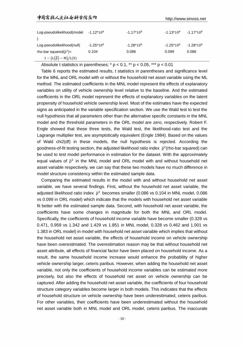
(III) Goodness-of-fit testing

To evaluate the performance of the above discrete choice models based on the

estimated sample, we are going to test the goodness-of-fit with the estimation of more

than one model structure. Following the evaluation criteria for data fit used by Bhat and

Pulugurta (1998), we use the adjusted likelihood ratio index ρ2(rho-bar squared ) defined

as follows:

ρ2 = 1 − [L(β) − M]/L(0)

where L(β) are the log-likelihood function values at convergence within the estimated

sample and M is the number of estimated parameters including the threshold parameters

in the ORL model and the alternative specific constants in the hybrid models. L(0) is the

log-likelihood values calculated with no parameters. Considering L(β) is a biased estimate

of the expectation over all samples, it is necessary to subtract M from L(β) and to remove

the effect of evaluating L(β) at the estimated values rather than for the true parameters

(Ben-Akiva and Swait 1986).

6, Results and discussion

(I) Model estimation results

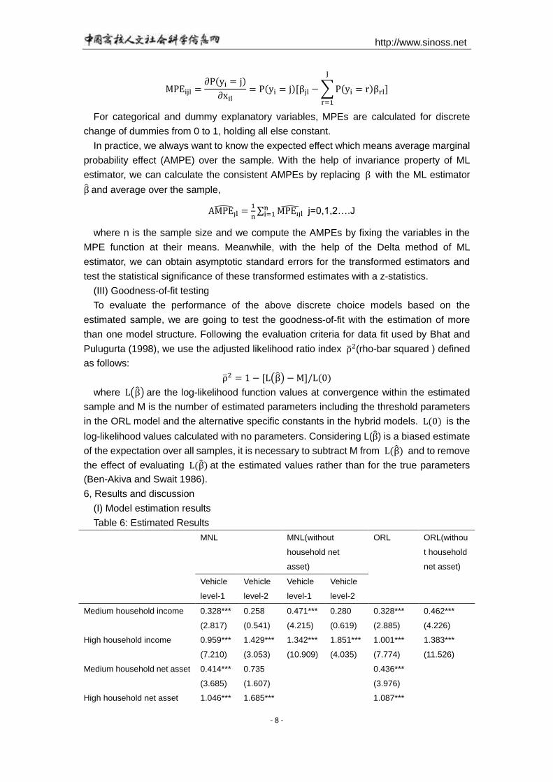
Table 6: Estimated Results

MNL MNL(without

household net

asset)

ORL ORL(withou

t household

net asset)

Vehicle

level-1

Vehicle

level-2

Vehicle

level-1

Vehicle

level-2

Medium household income 0.328*** 0.258 0.471*** 0.280 0.328*** 0.462***

(2.817) (0.541) (4.215) (0.619) (2.885) (4.226)

High household income 0.959*** 1.429*** 1.342*** 1.851*** 1.001*** 1.383***

(7.210) (3.053) (10.909) (4.035) (7.774) (11.526)

Medium household net asset 0.414*** 0.735 0.436***

(3.685) (1.607) (3.976)

High household net asset 1.046*** 1.685*** 1.087***


- 9 -

(7.765) (3.754) (8.343)

Married household with no

kids

1.730*** 0.074 1.269** 0.503 1.545*** 1.196**

(3.393) (0.091) (2.151) (0.605) (3.415) (2.207)

Married household with 1

kids

1.757*** 0.026 1.313** 0.549 1.569*** 1.242**

(3.488) (0.032) (2.275) (0.667) (3.518) (2.342)

Married household with 2 or

more kids

1.784*** 0.210 1.322** 0.522 1.615*** 1.252**

(3.470) (0.264) (2.271) (0.643) (3.545) (2.341)

Divorced or widowed

household

1.201** 0.006 0.735 0.351 1.045** 0.687

(2.147) (0.005) (1.166) (0.318) (2.076) (1.179)

Householder’s parent(s)

residing in the household

-0.314** -0.140 -0.294** -0.180 -0.291** -0.278**

(2.461) (0.432) (2.345) (0.556) (2.397) (2.327)

Administrative urban Hukou 0.001 -1.641**

*

0.128 -1.262**

*

-0.120 0.018

(0.010) (4.228) (1.228) (3.362) (1.144) (0.182)

Log of community population

density

-0.019 0.085* -0.007 0.093** -0.012 -0.000

(0.939) (1.690) (0.372) (2.089) (0.627) (0.001)

Number of workers in a

household

0.122*** 0.220* 0.148*** 0.283*** 0.130*** 0.160***

(2.875) (1.926) (3.514) (2.607) (3.230) (3.992)

Householder’s education

level

0.069* 0.042 0.109*** 0.051 0.062* 0.100***

(1.797) (0.330) (2.918) (0.419) (1.666) (2.777)

Householder’s age -0.029**

*

-0.036** -0.027**

*

-0.039**

*

-0.029*** -0.027***

(5.861) (2.488) (5.486) (2.762) (6.175) (5.861)

Transit accessibility 0.119 0.521* 0.169* 0.589** 0.157 0.208**

(1.187) (1.707) (1.722) (2.000) (1.621) (2.206)

Alternative specific constant -3.395**

*

-5.091**

*

-3.104**

*

-5.045**

*

(5.938) (4.483) (5.163) (4.654)

Threshold α1 3.183*** 2.964***

(6.185) (5.327)

Threshold α2 6.198*** 5.918***

(11.638) (10.346)

Number of observations 10,248 10,394 10,248 10,394

Wald chi2(df) 508.08(30) 455.92((26) 466.01(15

)

419.47(13)

Prob>chi 2(df) 0 0 0 0


- 10 -

Log-pseudolikelihood(model

)

-1.12*108 -1.17*108 -1.13*108 -1.17*108

Log-pseudolikelihood(null) -1.25*108 -1.28*108 -1.25*108 -1.28*108

rho-bar squared(ρ2)= 0.104 0.086 0.099 0.086

1 − [L(β) − M]/L(0)

Absolute t statistics in parentheses; * p < 0.1, ** p < 0.05, *** p < 0.01

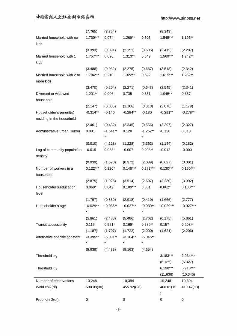
Table 6 reports the estimated results, t statistics in parentheses and significance level

for the MNL and ORL model with or without the household net asset variable using the ML

method. The estimated coefficients in the MNL model represent the effects of explanatory

variables on utility of vehicle ownership level relative to the baseline. And the estimated

coefficients in the ORL model represent the effects of explanatory variables on the latent

propensity of household vehicle ownership level. Most of the estimates have the expected

signs as anticipated in the variable specification section. We use the Wald test to test the

null hypothesis that all parameters other than the alternative specific constants in the MNL

model and the threshold parameters in the ORL model are zero, respectively. Robert F.

Engle showed that these three tests, the Wald test, the likelihood-ratio test and the

Lagrange multiplier test, are asymptotically equivalent (Engle 1984). Based on the values

of Wald chi2(df) in these models, the null hypothesis is rejected. According the

goodness-of-fit testing section, the adjusted likelihood ratio index ρ2(rho-bar squared) can

be used to test model performance in estimation for the dataset. With the approximately

equal values of ρ2 in the MNL model and ORL model with and without household net

asset variable respectively, we can say that these two models have no much difference in

model structure consistency within the estimated sample data.

Comparing the estimated results in the model with and without household net asset

variable, we have several findings. First, without the household net asset variable, the

adjusted likelihood ratio index ρ2 becomes smaller (0.086 vs 0.104 in MNL model, 0.086

vs 0.099 in ORL model) which indicate that the models with household net asset variable

fit better with the estimated sample data. Second, with household net asset variable, the

coefficients have some changes in magnitude for both the MNL and ORL model.

Specifically, the coefficients of household income variable have become smaller (0.328 vs

0.471, 0.959 vs 1.342 and 1.429 vs 1.851 in MNL model, 0.328 vs 0.462 and 1.001 vs

1.383 in ORL model) in model with household net asset variable which implies that without

the household net asset variable, the effects of household income on vehicle ownership

have been overestimated. The overestimation reason may be that without household net

asset attribute, all effects of financial factor have been placed on household income. As a

result, the same household income increase would enhance the probability of higher

vehicle ownership larger, ceteris paribus. However, when adding the household net asset

variable, not only the coefficients of household income variables can be estimated more

precisely, but also the effects of household net asset on vehicle ownership can be

captured. After adding the household net asset variable, the coefficients of four household

structure category variables become larger in both models. This indicates that the effects

of household structure on vehicle ownership have been underestimated, ceteris paribus.

For other variables, their coefficients have been underestimated without the household

net asset variable both in MNL model and ORL model, ceteris paribus. The inaccurate


- 11 -

estimation except the household income variable may come from that there are always

some kinds of relationship between the household net asset and these attributes. For

example, different household structure implies different household asset situation. If the

household net asset attribute is not involved in the explanatory variables, the estimation of

these household structure coefficients would be inaccurate. Therefore, the involvement of

household net asset in the model specification is a great improvement compared with

those studies without this attribute. This allows us to make a more precise explanation of

the household vehicle ownership decision.

By incorporating household annual income accompanied household net asset, we can

explain the vehicle ownership decision more comprehensively and elaborately from the

household financial effect perspective. Therefore, we do the analysis based on the

models with household asset variable. By setting the low household income as the

treatment group, we obtain significant and positive coefficient estimates of medium

household income and high household income variable in both models. And this indicates

that a higher household income or household net asset will raise the probability of

household owning one or more vehicles, holding other variables constant. For example,

for households in medium income and medium net category, such like the young

households, the average probabilities of owning 0, 1 and 1+ vehicle are 0.881, 0.113 and

0.007, respectively. Comparing the magnitudes of coefficients for the two income

categories (0.328 vs 0.959 and 0.258 vs 1.429 in MNL model, 0.328 vs 1.001 in ORL

model), we can see that a higher household income strengthen the utility or latent

propensity of a household owning one or more vehicles. Comparing estimated coefficients

in the household net asset variables with those in the household income variables, most

corresponding coefficients in medium category and high category of household net asset

variables are larger except the corresponding coefficients in vehicle level 2 in MNL model.

Firstly, the positive significant estimates imply that higher household net asset also

increases the probability of owning a higher vehicle level. Secondly, the higher

corresponding coefficient (0.328 vs 0.414 in medium category and 0.959 vs 1.046 in the

high category in vehicle level 1 alternative in MNL model) suggests that, holding all else

equal, when making their first vehicle ownership decision, the household net asset factor

takes priority of household annual income and which is also implied in the ORL model.

The same situation (1.429 vs 1.658 in the high category in vehicle level 1+ alternative in

MNL model) indicates that when deciding to purchase the second or more vehicles in a

household, the richer families, especially those families with higher household income and

net asset, also take the household net asset as a priority. The reason for this might be that

for those Chinese households who purchase their vehicles, they have accumulated a

certain amount of household capital and want to have a modern life with the household

vehicle. Under this situation, a household will not make the vehicle ownership decision

until they have enough net asset capability and under which the household net asset

takes the priority. The significant coefficients in high household income and net asset

variable imply that those rich households are more likely to purchase 2 or more vehicles.

Compared with previous works which only involve the household income factor (Kim and

Kim 2004, Chu 2002, Ryan J M 1999, …), the involvement of both household income and

net asset has made a progress in the comprehensive and intricate explanation of the


- 12 -

effects of financial factor on household vehicle ownership decision by decomposing it into

two correlated variables And by doing this, the different effects have been tested in this

study.

A second group of categorical variables are life-cycle stage and composite based

household structure determinants. Five household structures enter into the specification:

unmarried household, married household with no kid, married household with 1 kid,

married household with 2 or more kids and the divorced or widowed household. To avoid

the collinearity problem, we set the unmarried household as the baseline. As the

estimated results show, all positive coefficients for vehicle level 1 in MNL model are

significant. This indicates that compared with the unmarried household, other households

are more likely to own one vehicle. This is also true in the ORL model. Comparing the

increasing positive significant coefficients for the married household variables in the

vehicle 1 level, namely 1.730 vs 1.757 vs 1.784, we can find that as the household size

increases, the probability of owning 1 vehicle increases, too. The reason is the mobility

need coming from the children and adults. One aspect is the presence and number

increase of children; the other aspect is the household income and mobility needs

associated with more adults compared with the unmarried household. By comparing the

difference in the three coefficients, we can find that the two differences, 0.027 vs 0.027,

are equal. This implies that the effects of adding kid from 0 to 1 are the same with that in

adding kids from 1 to more. This implication highlights the important consideration of

children on vehicle ownership. Considering the release of the one-child policy in China,

there would be an increase in the vehicle demand in the next few years. Comparing the

coefficient in the divorced or widowed household, 1.201, the smaller coefficient indicates

that compared with the unmarried household, this household are more likely to own 1

vehicle, but compared with other married households, the probability of owning 1 vehicle

decreases. The main reason of this result may be that compared with the unmarried

household, the widowed or divorced household usually has more experienced workers

because of the later life-cycle stage which provides a better affordability for vehicle

ownership. This may also come from the stability of life or property acquisition from

divorce or inheritance. The lower probability compared with married household may be

that there are more working adults in the married household who not only earn more

household income but also need more mobility.

The administrative urban Hukou variable is a dummy and equals 1 if a household is

classified into the urban Hukou system, otherwise 0, based on the administrative

urban-rural division system announced in the 1950s. An insignificant coefficient in the

level 1 alternative in MNL model implies that for those families purchasing their first

vehicle, the administration system is no longer effective. This might be the fact that the

tremendous economic growth and rapid urbanization have made the administrative

urban-rural division system out of date. And this is especially true for the new rich families

who make the first vehicle ownership decision both in the urban and rural administrative

system. However, the significant negative coefficient -1.641 indicates this administrative

division system is still valid and the likelihood of owning two or more vehicle decreases

when a household is in the administrative urban system. The reason of this differentiation

might be that families owning two or more vehicles account for a relatively small


- 13 -

percentage.

(II) Average marginal probability effect analysis

Table 7: Average Marginal Probability Effect of MNL model

MNL ORL

(0) (1) (1+) (0) (1) (1+)

Medium household income -0.031*** 0.030*** 0.001 -0.031*** 0.029*** 0.002***

(2.836) (2.773) (0.403) (2.879) (2.875) (2.721)

High household income -0.094*** 0.085*** 0.009*** -0.096*** 0.088*** 0.007***

(7.694) (7.071) (2.684) (7.827) (7.813) (5.404)

Medium household net asset -0.041*** 0.037*** 0.005 -0.042*** 0.038*** 0.003***

(3.921) (3.563) (1.375) (3.957) (3.960) (3.453)

High household net asset -0.104*** 0.093*** 0.011*** -0.104*** 0.096*** 0.008***

(8.316) (7.594) (2.992) (8.377) (8.388) (5.482)

Married household with no kids -0.156*** 0.158*** -0.002 -0.148*** 0.136*** 0.011***

(3.348) (3.372) (0.345) (3.391) (3.387) (3.116)

Married household with 1 kids -0.158*** 0.160*** -0.002 -0.150*** 0.139*** 0.011***

(3.438) (3.471) (0.418) (3.496) (3.492) (3.197)

Married household with 2 or

more kids

-0.161*** 0.163*** -0.001 -0.154*** 0.143*** 0.012***

(3.446) (3.448) (0.199) (3.525) (3.520) (3.218)

Divorced or widowed

household

-0.108** 0.110** -0.002 -0.100** 0.092** 0.008**

(2.112) (2.139) (0.216) (2.067) (2.066) (2.000)

Householder’s parent(s)

residing in the household

0.029** -0.028** -0.001 0.028** -0.026** -0.002**

(2.467) (2.449) (0.233) (2.396) (2.396) (2.283)

Administrative urban Hukou 0.009 0.003 -0.012*** 0.011 -0.011 -0.001

(0.929) (0.261) (3.831) (1.145) (1.147) (1.107)

Log of community population

density

0.001 -0.002 0.001* 0.001 -0.001 -0.000

(0.661) (1.009) (1.736) (0.627) (0.627) (0.628)

Number of workers in a

household

-0.012*** 0.011*** 0.001* -0.012*** 0.012*** 0.001***

(3.120) (2.793) (1.665) (3.225) (3.229) (2.921)

Householder’s education level -0.006* 0.006* 0.000 -0.006* 0.005* 0.000

(1.804) (1.781) (0.218) (1.665) (1.665) (1.629)

Householder’s age 0.003*** -0.003*** -0.000** 0.003*** -0.003*** -0.000***

(6.076) (5.697) (1.992) (6.102) (6.091) (4.752)

Transit accessibility -0.014 0.010 0.004 -0.015 0.014 0.001

(1.471) (1.103) (1.573) (1.619) (1.620) (1.564)

Absolute z statistics in parentheses; * p < 0.1, ** p < 0.05, *** p < 0.01

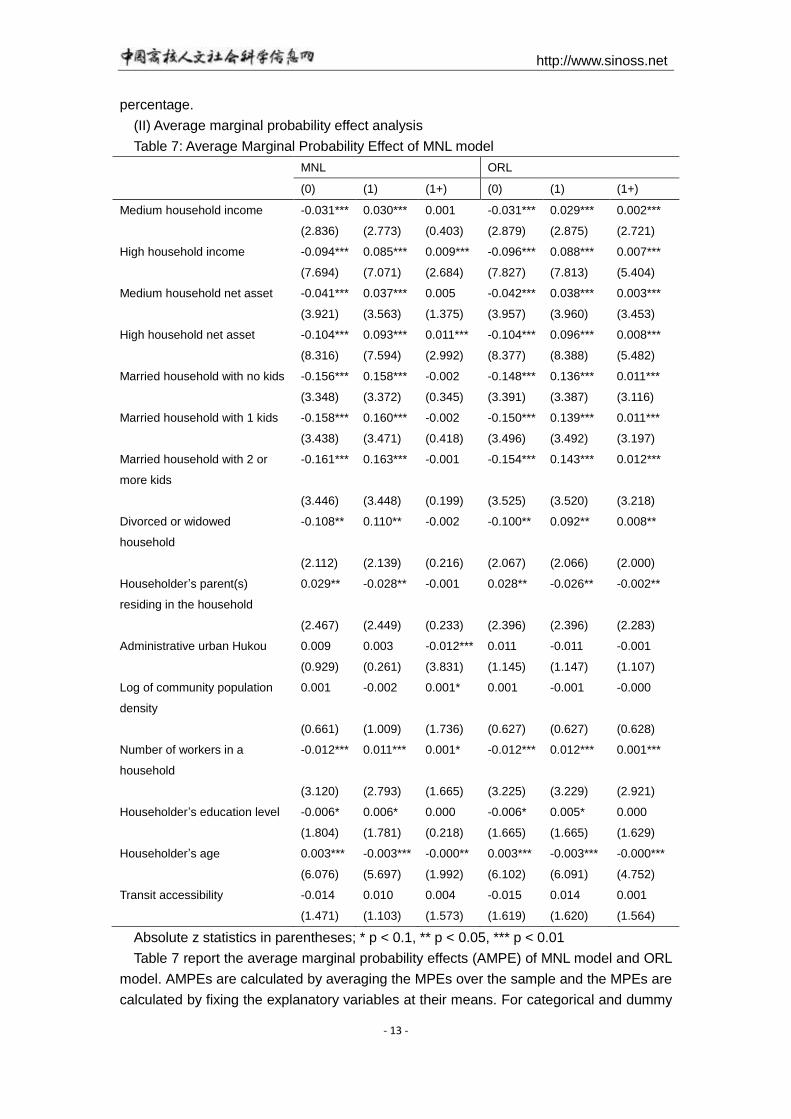
Table 7 report the average marginal probability effects (AMPE) of MNL model and ORL

model. AMPEs are calculated by averaging the MPEs over the sample and the MPEs are

calculated by fixing the explanatory variables at their means. For categorical and dummy


- 14 -

explanatory variables, MPEs are the discrete change in probability of owning the specific

vehicle level with respect to discrete change of dummies from 0 to 1, holding all else

constant. These estimates show the average marginal effects of one unit increase in the

factor on the probability of household vehicle ownership level while holding all other

variables constant. Totally, the AMPEs of one factor must sum up to be zero and the

reduced probability in one alternative equals the sum of other probability changes in other

alternatives. As we can see from the table, most of the estimates are significant at a high

percentage level and the signs are consistent with what those estimated coefficients imply

in Table 6. There is no much difference for these AMPE estimates in the two models.

Based on the estimates in Table 7, the AMPEs of variables on the probability of owning 2

or more vehicle are extremely minimal and this indicates that 1 vehicle may be the upper

bound on household vehicle ownership level for the majority households in modern China.

This finding is also consistent with what the frequency distribution of household vehicle

ownership level implies.

Accompanied with household net asset, we can get the more precise AMPE estimates

with respect to household income variable. The significant negative AMPEs in the vehicle

0 alternative imply that following an increase in the financial factors, on average, the

probability of owning 0 vehicle level would fall down and the significant positive estimates

in the other two vehicle level classes show an opposite implication. We test the null

hypothesis that the different household income and net asset groups have the same

AMPEs of vehicle ownership. With the rejection of these null hypothesizes, we can say

that different household income and net asset categories have differential effects on

vehicle ownership. For example, when a household is in the high household net asset

group, on average, the probability of owning 0 vehicle would decrease by about 10.4%

and the probability of having one vehicle would go up by 9.3% and having two or more

vehicles would go up by 1.1%. The relative moderate higher absolute magnitudes of

parameters in the household net asset variables also indicate that compared with

household income, in general, the household net asset plays a relative moderate more

important role in the household vehicle ownership decision.

6, Additional consideration

All above explanatory variables are characteristics of households. The value of these

variables varies across households. They can capture the explanatory power associated

with the households. In the MNL model, the alternative specific constants can capture the

unobserved explanatory power associated with household vehicle ownership including the

maintenance fees and operation fees. To enhance the explanatory power of the model,

this study also introduces a choice specific attribute variable: the monthly transport

expenditure. This variable varies across both households and vehicle level alternatives.

The monthly transport expenditure includes the vehicle maintenance fee, vehicle energy

cost and public transport expense.

In the CFPS survey, one household only report the real transportation expenditure

associated with the household vehicle ownership level. For example, if one household has

1 vehicle, then the reported transportation expenditure is the expense associated with 1

vehicle in this household. However, the hybrid model of MNL and CL specification requires

different transportation expenditures associated with different vehicle ownership in this


- 15 -

household. Based on the specification of the dependent variable, there should be three

transportation expenditures within each individual household. For example, the three

transportation expenditures associated with the 1 vehicle household are 0 vehicle

transportation expenditure, 1 vehicle transportation expenditure and 2 vehicles

transportation expenditure. Among these three expenditures, only the expenditure

associated with 1 vehicle is the reported value and the other expenditures need to be

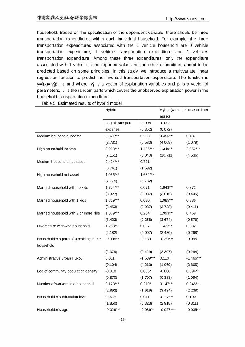
predicted based on some principles. In this study, we introduce a multivariate linear

regression function to predict the invented transportation expenditure. The function is

y=f(x)= vi′β + ε and where vi

′ is a vector of explanation variables and β is a vector of

parameters, ε is the random parts which covers the unobserved explanation power in the

household transportation expenditure.

Table 5: Estimated results of hybrid model

Hybrid Hybrid(without household net

asset)

Log of transport

expense

-0.008

(0.352)

-0.002

(0.072)

Medium household income 0.321*** 0.253 0.455*** 0.487

(2.731) (0.530) (4.009) (1.079)

High household income 0.958*** 1.426*** 1.340*** 2.052***

(7.151) (3.040) (10.711) (4.536)

Medium household net asset 0.424*** 0.731

(3.741) (1.592)

High household net asset 1.056*** 1.682***

(7.775) (3.732)

Married household with no kids 1.774*** 0.071 1.948*** 0.372

(3.327) (0.087) (3.616) (0.445)

Married household with 1 kids 1.819*** 0.030 1.985*** 0.336

(3.453) (0.037) (3.728) (0.411)

Married household with 2 or more kids 1.839*** 0.204 1.993*** 0.469

(3.423) (0.258) (3.674) (0.576)

Divorced or widowed household 1.268** 0.007 1.427** 0.332

(2.182) (0.007) (2.430) (0.298)

Householder’s parent(s) residing in the

household

-0.305** -0.139 -0.295** -0.095

(2.379) (0.429) (2.307) (0.294)

Administrative urban Hukou 0.011 -1.639*** 0.113 -1.466***

(0.104) (4.213) (1.069) (3.805)

Log of community population density -0.018 0.086* -0.008 0.094**

(0.870) (1.707) (0.383) (1.994)

Number of workers in a household 0.123*** 0.219* 0.147*** 0.248**

(2.892) (1.919) (3.434) (2.238)

Householder’s education level 0.072* 0.041 0.112*** 0.100

(1.850) (0.323) (2.918) (0.811)

Householder’s age -0.029*** -0.036** -0.027*** -0.035**


- 16 -

(5.800) (2.487) (5.512) (2.441)

Transit accessibility 0.116 0.520* 0.173* 0.613**

(1.139) (1.703) (1.726) (2.036)

Alternative specific constant -3.470*** -5.052*** -3.749*** -5.334***

(5.844) (4.451) (6.313) (4.791)

Number of observations 10,116 10,166

Wald chi2(df) 508.58(31) 439.75(27)

Prob>chi 2(df) 0 0

Log pseudolikelihood(model) -1.11*108 -1.13*108

Log-pseudolikelihood(null) -1.25*108 -1.25*108

rho-bar squared(ρ2)= 0.112 0.099

1 − [L(β) − M]/L(0)

Absolute t statistics in parentheses; * p < 0.1, ** p < 0.05, *** p < 0.01

Based on the renewed dataset, we use the ML method to do the estimation of the hybrid

model. We do the estimations with and without household net asset variable, too. As we

can see from the estimated results, the hybrid model with household net asset variable

performs better than model without this financial factor. Meanwhile, the coefficients of

household income variables are also overestimated in the model without household net

asset. The effects of household income on vehicle ownership are overestimated. For

other variables, the coefficients in model without household net asset have overestimation

or underestimation problems, too. Therefore, it is necessary to involve the household net

asset in model specification, especially considering the primary effects of household

financial factor on vehicle ownership.

By adding the choice specific variable, the hybrid model indeed fits the survey sample

better than MNL model and ORL model based on the adjusted likelihood ratio index.

However, the improvement is relatively small. Meanwhile, there isn’t too much difference

in the coefficients of all explanatory variables other than the transportation expenditure

variable between the MNL model and hybrid model. And they have the same significance

level in coefficients and Wald chi 2 value. In the hybrid mode with household net asset, the

coefficient of transportation expenditure variable is insignificant -0.008 which has an

anticipated sign. The reason for above results may be that 2/3 transportation expenditures

in the renewed dataset are predicted based on the regress function, not the real ones.

Restricted by the inadequate data, we can get the moderate results which give a better

way to model the household vehicle ownership.

5, Conclusions

With the tremendous economic growth and rapid urbanization since the economic

reform, the Chinese families have accumulated huge wealth and grown into a huge

consumer group. Vehicle has been seen as the symbol of modern life and becomes one of

their important durables especially considering its connection with travel mode choice,

destination and residential location. However, problems with the growth of vehicle volume

has occurred, suck like the traffic accidents, traffic congestion, air pollution. To probe into

the household vehicle ownership decision process, this study uses disaggregate models

to explore the relationship of household vehicle ownership and the latent determinants at

the household level.


- 17 -

1, By using disaggregate models, we can capture the effects of explanatory variables

on household vehicle ownership at the household decision maker unit level. By involving

explanatory attributes of household and its residents, this gives us a more intuitively

credible, precise and effective analysis at the disaggregate level. Furthermore, the CFPS

survey allows us to explore the latent determinants of household vehicle ownership at the

disaggregate level across the whole nation. This study contributes a lot to empirical work

of household vehicle ownership in China.

2, Compared with existing literatures, this study decompose the household financial

factor into household income variable and household net asset variable. By adding the

household net asset attribute in model specification, we find that the effects of household

income on vehicle ownership are smaller than those indicated by model without

household net asset attribute. Meanwhile, caused by the relationship between household

net asset and other household attributes, effects of other variables on vehicle ownership

become different when adding household net asset attribute. Therefore, we believe

without household net asset attribute, there is misestimating of the effects of explanatory

variables in household vehicle ownership studies. Additionally, models fit the estimated

sample dataset better when adding the household net asset variable which highlights the

importance of net asset on vehicle ownership. Another advantage of adding household

net asset variable is that we can capture the effects of household financial factor on

vehicle ownership more comprehensively and precisely by the decomposition. This

finding provides policy makers and vehicle manufacturers some inspirations on the real

effects of the influence factors on household vehicle ownership.

3, Based on the estimated results of different models and AMPEs, the household

income variables, household net asset variables and household structure variables show

larger effects on vehicle ownership. Therefore, the household affordability and demand

consideration are the two primary determinants for household vehicle ownership among

the explanatory attributes.

4, For the two household financial composites, based on the estimated results, we

conclude the household net asset consideration takes priority over household income

consideration in household vehicle ownership decision. This may come from that as a

durable good, vehicle purchase is still an expensive expenditure at present in China. So

for policy consideration associated with household vehicle ownership in China, not only

income increase, but also household net asset growth should be under consideration.

5, Entering the marriage stage has great positive effects on household 1 vehicle

ownership based on the estimates of household structure variables. One reason may be

that after entering the marriage stage, workers in the household double which results in

household income and mobility needs doubling. Additionally, mobility needs of children

impose positive effects on 1 vehicle ownership, both from 0 to 1 kid and from 1 kid to more

kids. Therefore, the release of one-child policy is expected to enlarge the vehicle market

to some extent.

6, Based on the estimated results, one vehicle may be the upper bound on household

vehicle ownership for the majority families in this sample dataset. Meanwhile, the

administrative urban-rural division system is no longer effective in household 1 vehicle

ownership decision.


- 18 -

7, Based on the goodness-of-fit, there isn’t too much difference in model performance

for the MNL model and ORL model within the estimated sample data. Furthermore, we

apply a hybrid model of MNL model and CL model to involving the choice specific

transportation expenditure attribute. This has provided a better way to understand the

household vehicle ownership decision process.

These findings have some empirical implications for vehicle manufacturers and policy

makers. First, considering the misestimating in empirical household vehicle ownership

studies without household net asset attribute, the policy and plans based on the estimated

results should be adjusted to avoid the wasting of resources. Second, considering the

priority of household net asset on vehicle ownership and the comprehensive effects of

household financial factors, both of the two financial composites should be under

consideration when making policies and production plans. Third, to pursue higher profits,

vehicle manufacturers and sellers should adjust the production and selling plans by

focusing on families who decide to own their first vehicle. Specifically, the new marriage

households are more likely to own their first vehicle. And they should pay the same

attention to households receiving two-child policy as those with their first child. Forth,

when making policies and plans, the administrative urban-rural division system should not

be under consideration. Instead, policy makers and manufacturers should pay attention to

other attribute associated with the urban and rural division, such like the residential

location.


- 19 -

Reference

[1] Ben-Akiva, M. and J. Swait (1986). "The Akaike likelihood ratio index." Transportation Science 20(2):

133-136 %@ 0041-1655.

[2] Ben-Akiva, M. E. and S. R. Lerman (1985). Discrete Choice Analysis : Theory and Application to

Travel Demand. Cambridge, Mass, The MIT Press.

[3] Bhat, C. R. and V. Pulugurta (1998). "A comparison of two alternative behavioral choice

mechanisms for household auto ownership decisions." Transportation Research Part B:

Methodological 32(1): 61-75 %@ 0191-2615.

[4] Chu, Y.-L. (2002). "Automobile ownership analysis using ordered probit models." Transportation

Research Record: Journal of the Transportation Research Board(1805): 60-67 %@ 0361-1981.

[5] Clark, S. D. (2009). "The determinants of car ownership in England and Wales from anonymous

2001 census data." Transportation Research Part C: Emerging Technologies 17(5): 526-540.

[6] Dargay, J. and D. Gately (1999). "Income's effect on car and vehicle ownership, worldwide: 1960–

2015." Transportation Research Part A: Policy and Practice 33(2): 101-138.

[7] Dargay, J. and M. Hanly (2007). "Volatility of car ownership, commuting mode and time in the UK."

Transportation Research Part A: Policy & Practice 41(10): 934-948.

[8] Dargay, J. M. (2001). "The effect of income on car ownership: evidence of asymmetry."

Transportation Research Part A Policy & Practice 35(9): 807-821.

[9] De Jong, G., J. Fox, A. Daly, M. Pieters and R. Smit (2004). "Comparison of Car Ownership

Models." Transport Reviews 24(4): 375-408.

[10] Engle, R. F. (1984). "Chapter 13 Wald, likelihood ratio, and Lagrange multiplier tests in

econometrics." Handbook of Econometrics 2(84): 775-826.

[11] Giuliano, G. and J. Dargay (2006). "Car ownership, travel and land use: a comparison of the US and

Great Britain." Transportation Research Part A: Policy and Practice 40(2): 106-124 %@ 0965-8564.

[12] Hao, H., H. Wang and R. Yi (2011). "Hybrid modeling of China’s vehicle ownership and projection

through 2050." Fuel & Energy Abstracts 36(2): 1351-1361.

[13] Holtzclaw, J., R. Clear, H. Dittmar, D. Goldstein and P. Haas (2002). "Location Efficiency:

Neighborhood and Socio-Economic Characteristics Determine Auto Ownership and Use - Studies

in Chicago, Los Angeles and San Francisco." Transportation Planning & Technology 25(1): 1-27.

[14] Karlaftis, M. and J. Golias (2002). "Automobile ownership, households without automobiles, and

urban traffic parameters: Are they related?" Transportation Research Record: Journal of the

Transportation Research Board(1792): 29-35 %@ 0361-1981.

[15] Kim, H. S. and E. Kim (2004). "Effects of public transit on automobile ownership and use in

households of the USA." Review of Urban & Regional Development Studies 16(3): 245-262 %@

1467-1940X.

[16] Li, J., J. Walker, S. Srinivasan and W. Anderson (2010). "Modeling private car ownership in China:

investigation of urban form impact across megacities." Transportation Research Record: Journal of

the Transportation Research Board(2193): 76-84 %@ 0361-1981.

[17] Nolan, A. (2010). "A dynamic analysis of household car ownership." Transportation Research Part A

Policy & Practice 44(6): 446-455.

[18] Potoglou, D. and P. S. Kanaroglou (2008). "Modelling car ownership in urban areas: a case study of

Hamilton, Canada." Journal of Transport Geography 16(1): 42-54 %@ 0966-6923.

[19] Prevedouros, P. D. and J. L. Schofer (1993). "Factors affecting automobile ownership and use."

Population 31(37.8): 34.35.


- 20 -

[20] Riley, K. (2002). "Motor Vehicles in China: The Impact of Demographic and Economic Changes."

Population & Environment 23(5): 479.

[21] Schimek, P. (1996). "Household motor vehicle ownership and use: How much does residential

density matter?" Transportation Research Record: Journal of the Transportation Research

Board(1552): 120-125 %@ 0361-1981.

[22] Scott, D. M. and K. W. Axhausen (2006). "Household Mobility Tool Ownership: Modeling

Interactions between Cars and Season Tickets." Transportation 33(4): 311-328.

[23] Tang, R. (2009). The Rise of China's Auto Industry and Its Impact on the U.S. Motor Vehicle

Industry.

[24] Tardiff, T. J. (1980). "Vehicle choice models: review of previous studies and directions for further

research[J]." Transportation research Part A: General 14(5-6): 327-336.

[25] Wang, F. and D. Wang (2014). "A disaggregate study of household car ownership in Chinese large

cities: a case study of Beijing." 人文地理 29(5): 75-80.

[26] Whelan, G. (2007). "Modelling car ownership in Great Britain." Transportation Research Part A:

Policy & Practice 41(3): 205-219.

[27] Winkelmann, R. and D. V. S. Boes (2006). "Analysis of Microdata." (12): B655-B662.

[28] Xie, Y. and J. Hu (2014). "An introduction to the China family panel studies (CFPS)." Chinese

Sociological Review 47(1): 3-29 %@ 2162-0555.

[29] Zhang, Z., W. Jin, H. Jiang, Q. Xie, W. Shen and W. Han (2017). "Modeling heterogeneous vehicle

ownership in China: A case study based on the Chinese national survey." Transport Policy 54:

11-20.


- 21 -

A disaggregate analysis for determinants of household vehicle

ownership level in China

Shao Changkai

(Center for Economics, Finance and Management Studies, Hunan University, Changsha / Hunan,

410006)

Abstract: Considering the rapid growth in economics and vehicle ownership volume, a comprehensive

and precise understanding of household vehicle ownership is of vital importance in China. In this study,

we employ the multinomial logit model(MNL) and ordered logit model(ORL) to investigate the

determinants of household vehicle ownership at the disaggregate level across the whole nation based on

the China Family Panel Studies(CFPS) data. By decomposing the household financial attribute, we

introduce the categorical household income variables and categorical household net asset variables in

model specification accompanied with categorical household structure variables and other influential

factors. The results show that with household net asset, we can get a more precise estimation, especially

for household income variables. After adding household net asset, the effects of household income on

vehicle ownership are smaller than those indicated by model without household net asset. Meanwhile,

caused by relationship between household net asset and other attributes, other variables show different

effect on household vehicle ownership, too. Based on results with household net asset, the household

financial attribute and structure characteristic are the two primary affordability and demand determinants.

Entering marriage stage and mobility of kids impose positive effects on 1 household vehicle ownership.

The administrative urban-rural division system is ineffective in household vehicle ownership within this

sample data. For the two models, there isn’t too much difference in model performance within the

estimated data. Furthermore, by constructing the choice specific transportation expenditure variable, we

apply the hybrid model of MNL and conditional logit(CL) model to understand the household vehicle

ownership better . In application, the results can be used to assist policy makers and vehicle

manufacturers to make policies and production plans more precisely and rationally.

Keywords: Household vehicle ownership, Disaggregate analysis, Financial factor decomposition,

Household structure characteristic, Hybrid model

中国家庭汽车拥有水平影响因子的非集计分析 · Taiwan, as well as Xinjiang, Tibet,...

Documents

Transcript of 中国家庭汽车拥有水平影响因子的非集计分析 · Taiwan, as well as Xinjiang, Tibet,...