BYDGOSZCZ – 2011

ZESZYTY NAUKOWE NR 259

ELEKTROTECHNIKA

16

UNIWERSYTET TECHNOLOGICZNO-PRZYRODNICZYIM. JANA I JÊDRZEJA ŒNIADECKICH

W BYDGOSZCZY

REDAKTOR NACZELNYprof. dr hab. in¿. Janusz Prusiñski

REDAKTOR NACZELNY SERIIdr in¿. S³awomir Cieœlik

OPRACOWANIE TECHNICZNEmgr in¿. Daniel Morzyñski

© CopyrightWydawnictwa Uczelniane Uniwersytetu Technologiczno-Przyrodniczego

Bydgoszcz 2011

ISSN 0209-0570

Wydawnictwa Uczelniane Uniwersytetu Technologiczno-Przyrodniczegoul. Ks. A. Kordeckiego 20, 85-225 Bydgoszcz, tel. 52 3749482, 3749426

e-mail: wydawucz@utp.edu.pl http://www.wu.utp.edu.pl

Wyd. I. Nak³ad 80 egz. Ark. aut. 2,3. Ark. druk. 2,6.Zak³ad Ma³ej Poligrafii UTP Bydgoszcz, ul. Ks. A. Kordeckiego 20

Contents

1. Piotr Mysiak, Piotr Grugel – A diode rectifier with coupled reactor and small shunt power filter ........................................................................................................ 5

2. Sławomir Andrzej Torbus, Andrzej Jordan, Dariusz Surma – Verification of a mathematical model of the polarimetric current sensor with single-mode fiber measurement coil based on computer simulation by finite element method ..................................................................................................................... 17

3. Piotr Grugel – The use of complex sliding window Discrete Fourier Transformation in current and voltage distortion analysis in three-phase circuits ...................................................................................................................... 27

UNIWERSYTET TECHNOLOGICZNO-PRZYRODNICZY IM. JANA I JĘDRZEJA ŚNIADECKICH W BYDGOSZCZY

ZESZYTY NAUKOWE NR 259 ELEKTROTECHNIKA 16 (2011) 5-16

A DIODE RECTIFIER WITH COUPLED REACTOR AND SMALL

SHUNT POWER FILTER

Piotr Mysiak1, Piotr Grugel2

1 Gdynia Maritime University ul. Morska 81-87, 81-225 Gdynia

e-mail: mysiak@am.gdynia.pl

2 University of Technology and Life Sciences Al. S. Kaliskiego 7, 85-796 Bydgoszcz

e-mail: p.gr@utp.edu.pl

Summary: The article describes the laboratory and simulation tests of 12- and 24-pulse power grid converter systems with DC voltage output that work together with shunt active power filter (APF). It presents both the operations' principles and the results of these tests. The systems under discussion make it possible to reduce the number of unwanted higher harmonics in the power network current. Moreover, they can also help eliminate the 23- and 25-order harmonics especially in the conditions of local power network supply. In order to obtain the multi-pulsed system's operation, a set of coupled three-phase power network reactors (CTR) has been used.

Keywords: Active power filters, coupled three-phase power network reactors, local power network, multi-pulse grid converters, power conditioning.

1. INTRODUCTION

Supplying a rectifier from grid generates unwanted, higher harmonics of the network current. With the increase in the number of converter’s pulses, THD coefficient of the network current decreases, according to n=kp±1 formula, where n stands for the index of generated harmonic, p is the number of converter pulses and k represents any natural number. In order to filter higher current harmonics, Active Power Filter (APF) can be used. The power of APF has to be proportional to distortion power. Increasing the number of converter’s pulses, for example, with the aid of a set of properly paired coupled power network reactors, one obtains the reduction of distortion power. Consequently, it makes the use of smaller gabarits of the Active Power Filter possible.

6 P. Mysiak, P. Grugel

2. SYSTEM DESCRIPTION

The project concerns a current topic of power-electronic conversion of the AC power drawn from a supply line, without negative effect of the converter on this line [4]. Along with more and more popular converters realised with the aid of full-controlled semiconductor elements, such as power transistors and GTO thyristors, controlled by using pulse width modulation techniques, there is a possibility to build power-electronic converters, which convert the energy of the AC into that of the DC with the aid of a set of properly paired coupled reactors installed between the supply line and the semiconductor rectifier. Proper magnetic pairings and proper pairing of reactor windings makes it possible to convert the three-phase voltage system of the supply line into the system with a larger number of phases without the use of transformers. At the same time, the power of the three-phase coupled reactors is several times lower than that of classical converter transformers. Minimisation of the supply line current deformation is obtained by using a system of coupled power network reactors, the task of which is to increase the number of phases of the converter input voltage with the aid of diodes or conventional thyristors.

The coupled reactors play here a similar role to that of the converter transformers revealing a complicated system of secondary windings; however the power of the reactors is several times smaller. To improve the system power factor and THD coefficient, the small shunt active power filter was implemented by using a three-phase voltage-source IGBT inverter. The filter was also applied to the multi-pulse converter with CTR. The harmonic content, and reactive power absorption of described converter system are significantly reduced by both CTR and shunt active filter. This shunt active power filter is composed of two distinct elements: 1) the PWM converter (power circuit) 2) the active filter controller.

In order to reproduce accurately the compensating currents, the PWM converter should have a high switching rate. Normally, f PWM > 10f hmax , where f hmax represents the frequency of the highest load current harmonic to be compensated. Both voltage-source (VSI) [1] and current-source (CSI) inverters can be used to implement a shunt active filter. Although they are similar to the PWM inverters used for ac motor drives, unlike the PWM inverters for shunt active filters, which must behave as a non-sinusoidal current source, almost all shunt active filters in commercial operation use voltage-source inverters. All experimental results presented in this work were obtained from a prototype realized with a VSI. Fig.1a shows the basic configuration of a shunt active filter [8], [9]. It comprises a voltage-source inverter (VSI) with PWM current control (hysteresis control) and an active filter controller that realizes almost instantaneous control algorithm. The shunt active filter works in a closed-loop, sensing continuously the load current i and calculating the instantaneous values of the compensating current reference i*k for the PWM converter. If the switching ratio of the PWM converter is high enough, the current ik will contain high frequency harmonics, that can be easily filtered out using small high-pass filters. In an ideal case, the PWM converter may be considered as a linear power amplifier, where the compensating current ik tracks strictly its reference i*k. The control algorithm implemented in the shunt active filter controller determines the compensation characteristics of the shunt active filter.

A diode rectifier with coupled reactor and small shunt power filter 7

Fig. 1. Basic configuration of the shunt active filter (a) and schematic diagram of 12-pulse diode rectifier with CTR coupled reactor system and shunt active power filter (b)

Fig. 1b presents a basic concept of a 12-pulse converter, in which the use of three-phase coupled reactors with shunt active filter allows for generation of two phase-shifted systems of three-phase voltages making the input parameters for two 6-pulse rectifiers. For the time being, examples discussed in the literature mostly apply similar 12-pulse system, however with no active filters for doubling the numbers of input voltage phases in voltage inverters supplying induction machines. Moreover, the literature has not yet provided either detailed analysis concerned with operation of such a system, or guides concerning its design algorithms. Unlikely previously discussed examples, the work included the analysis, which further constituted the basis for designing the 12-pulse system and allowed for analyzing the effect of supply line parameters, including its impedance, on the operation of the system. The researchers also developed a fragment of the general theory of improved systems with coupled reactors, which allowed synthesis of systems with increased numbers of voltage phases.

a)

b)

8 P. Mysiak, P. Grugel

Simulation tests were carried out to examine the possibility of the use of the system as a supply source in intermediate frequency converters for voltage inverters.

The methods for described system examination included theoretical analysis, simulation tests and model tests of a real converter containing two 6-pulse bridge systems supplied from a three-phase power network via a system of shunt active filter with coupled three-phase power network reactors. As it was expected, the currents drawn from the supply line had almost a sine form, of course not typical form of classical 12-pulse rectifiers, realised using three-phase converters. The test results not only can be used for verification of the developed design algorithms for the examined class of converters, they also allow for studying possibilities of application of the examined converter in the DC and AC driving systems. Because of the requirement of high reliability level they can be used especially in the marine applications.

The overall work aimed at developing a design method for power-electronic converters that would convert alternate voltage into one-way voltage, and would be equipped with a system of three-phase coupled reactors having the form close to a sine curve, which secure consumption of the current. This included simulation and laboratory tests, for which laboratory models of a 2-kVa 12-pulse and 24-pulse converters systems with shunt active filter were designed and constructed. The realisation of the issue has made it possible to formulate a more precise theory of and develop a design methodology for power-electronic converters used for converting the energy of the AC into that of the DC. A significant feature of these converters is reduced consumption of the deformation power.

The essential issues associated with the realisation of the above indicated research tasks included: • Developing a mathematical model of the system and determining analytical and

synthesizing relations that allow formulation of a design procedure for a converter which would consist of a system of three-phase coupled reactors, two in-parallel paired rectifier bridges and shunt active power filter

• Working out a simulation model and carrying our detailed simulation tests of the system, to create the basis for verification of the theoretical results and final formulation of the conditions to be met by a magnetic system of reactors and the set of properly configured power semiconductor elements

• Experimental verification of the results of the theoretical analysis and simulation tests, complemented by the interpretation of the obtained results.

The 12-pulse diode rectifier presented in the Fig.1b is supplied from a three-phase power network with the phase voltage Un (n=a,b,c). The input circuit of the converter comprises linear power network reactors Ls, Ld, shunt active filter and coupled three-phase power network reactor CTR. Input terminals of the reactor CTR are connected with the supply network terminals through linear reactors Ls, Ld. Output terminals of the reactor CTR are, in turn, connected with phase branches of two three-phase diode bridge systems. The DC terminals of all bridge systems are connected in parallel to the filtering capacitor Co. The task of the set of the coupled reactors is to generate three alternating voltages UKn, of which waveforms take the sine shape when idling and the 12-step shape at load close to nominal. Voltages UKn, measured with respect to the input circuit star point N, can be interpreted as the quantities created in result of cyclic starts of the DC voltage 2Ed, via the switches of two bridges. Required condition to be met in order to obtain 12-step waveforms of voltages UKn is that all diodes must conduct the current during half of the voltage period of the supply line. The symmetry of the 12-step

A diode rectifier with coupled reactor and small shunt power filter 9

voltages UKn results directly from the phase shift angle, equal to 2π/12, between the conduction states of particular diodes in the two bridges. Input terminals Dmn (m = 1,3) of each of the two three-phase bridge systems reveal symmetrical three-phase voltages of the 6-step shape. Those two systems of three-phase voltage are relatively shifted by 2π/12, and therefore creating, via systems CTR, one 6-phase system. Thus, it can be assumed that due to a CTR, the three-phase line voltage has been transformed into 6-phase voltage. Moreover, two systems of three-phase currents imn are added up in reactors CTR and are converted into one three-phase system of currents in, drawn from the supply line. The waveforms of these currents are very close to a sine curve. Power network reactors Ld and shunt active filter additionally reduce, to a required level, higher-order harmonics of the currents in, generated by corresponding harmonics of the 12-step waveforms of three-phase voltages UKn.

Fig. 2. The results of simulation experiments concerned with 50 kW 6-pulse converter with power active filter (a), the results of simulation experiments concerned 50 kW 12-pulse converter with CTR system and power active filter (b) as well as the results of laboratory experiments on 2 kW 12-pulse converter only with CTR system (c)

a)

b)

c)

10 P. Mysiak, P. Grugel

3. SELECTED RESULTS OF THE SYSTEM

The Figure 2 presents the selected results of simulation and laboratory experiments – the results of simulation experiments concerned with 50kW 6-pulse converter with power active filter (a), the results of simulation experiments concerned 50kW 12-pulse converter with CTR system and power active filter (b) as well as the results of laboratory experiments on 2kW 12-pulse converter only with CTR system (c). The most important in Fig (b) is visibly small power of implemented shunt active filter. In the Fig (c) is remarkable that the distortion of the net current ia(1) is larger than in the case of current ia, illustrated in figure (b).

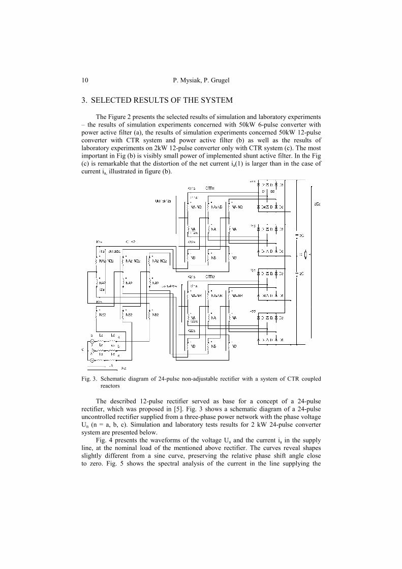
Fig. 3. Schematic diagram of 24-pulse non-adjustable rectifier with a system of CTR coupled

reactors

The described 12-pulse rectifier served as base for a concept of a 24-pulse rectifier, which was proposed in [5]. Fig. 3 shows a schematic diagram of a 24-pulse uncontrolled rectifier supplied from a three-phase power network with the phase voltage Un (n = a, b, c). Simulation and laboratory tests results for 2 kW 24-pulse converter system are presented below.

Fig. 4 presents the waveforms of the voltage Ua and the current ia in the supply line, at the nominal load of the mentioned above rectifier. The curves reveal shapes slightly different from a sine curve, preserving the relative phase shift angle close to zero. Fig. 5 shows the spectral analysis of the current in the line supplying the

A diode rectifier with coupled reactor and small shunt power filter 11

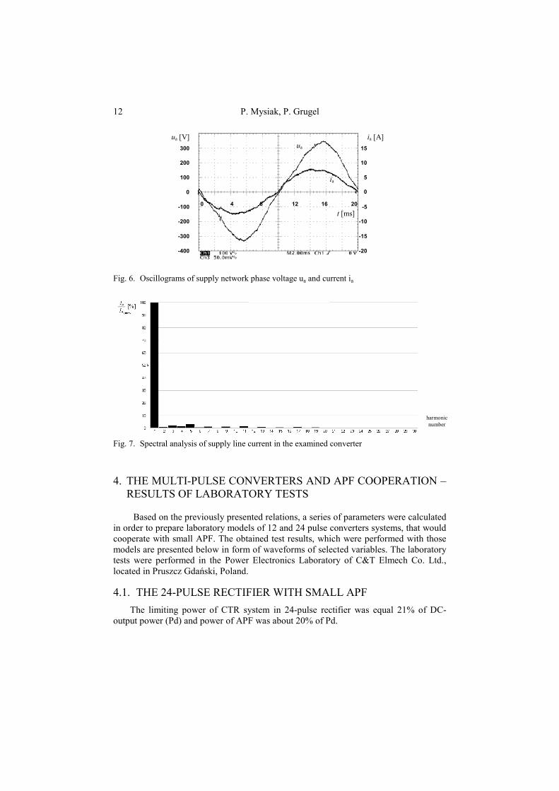
24-pulse converter. Of the highest significance is the fact that higher harmonics, of orders of 17, 19, are not practically recorded, while the harmonics of orders of 5, 7 and 23, 25 are significantly reduced. Fig.6 shows voltage and current oscillograms in the line supplying the 24-pulse converter, working in nominal load conditions. Noteworthy is relatively small deformation of the line current. That the oscillogram of the phase voltage in the supply network does not reveal deformations only confirms correct operation of the model system under nominal load conditions. Fig.7 presents a frequency spectrum of the current drawn from the supply network, with the percentage values of higher harmonics related to the basic harmonic. Calculated from formula:

100%II1W

1n

2hn

1hI ⋅= ∑

∞

⟩, (1)

THD coefficient is equal to 4,88%, which is considered to be very good. Moreover, Fig.7 reveals visible reduction of higher harmonics of orders of 5, 7, 11, 13, 17, 19, 23, and 25.

Fig. 4. Waveforms of power network phase voltage Ua and current ia

Fig. 5. Spectral analysis of the waveform of supply line current ia

ua [V]

t [ms]

ua

ia

0

5

10

-5

-10

ia [A]

harmonic number

Ia [A]

12 P. Mysiak, P. Grugel

Fig. 6. Oscillograms of supply network phase voltage ua and current ia

Fig. 7. Spectral analysis of supply line current in the examined converter

4. THE MULTI-PULSE CONVERTERS AND APF COOPERATION – RESULTS OF LABORATORY TESTS

Based on the previously presented relations, a series of parameters were calculated in order to prepare laboratory models of 12 and 24 pulse converters systems, that would cooperate with small APF. The obtained test results, which were performed with those models are presented below in form of waveforms of selected variables. The laboratory tests were performed in the Power Electronics Laboratory of C&T Elmech Co. Ltd., located in Pruszcz Gdański, Poland.

4.1. THE 24-PULSE RECTIFIER WITH SMALL APF The limiting power of CTR system in 24-pulse rectifier was equal 21% of DC-

output power (Pd) and power of APF was about 20% of Pd.

t [ms]

ia [A]

0 4 8 12 16 20

ua

ia

0

100

200

300

-100

-200

-300

-400

0

5

10

15

-10

-15

-20

-5

ua [V]

harmonic number

A diode rectifier with coupled reactor and small shunt power filter 13

Fig. 10. Power network current and harmonics after compensation.

Fig. 9. The compensating current waveforms and its harmonics

Fig. 8. Supply grid current and harmo-nics before compensation

14 P. Mysiak, P. Grugel

4.2. THE 12-PULSE RECTIFIER WITH SMALL APF The limiting power of CTR system in 12-pulse rectifier was equal 13% of Pd and

power of APF was about 20% of Pd.

Because of cooperation with APF, in both arrangements of multi-pulse converters,

application of linear reactors Ld may be disregarded, and thereby construction cost of the system decreases. The system of multi-pulse converter cooperating with the active filter allows to achieve supply current of minor distortion. At the same time it should be noticed that applied system of coupled reactors, as well as the active filter are characterized by low power, which testifies for their low costs. Practical application of the system may be considered with regards to local networks such as ship power networks, which more often supply non-linear receivers. However the application should take into account strict requirements to preserve parameters defining quality of energy. Exemplary network configuration, which supplies passenger ship is showed on the Figure 13.

Fig. 11. Power network current before compensation and compensating current

Fig. 12. Power network current and harmonics of supply grid current after compensation.

A diode rectifier with coupled reactor and small shunt power filter 15

Fig. 13. The scheme of passenger ship supply system

5. CONCLUSIONS

The concept of the rectifier system with coupled reactors and the active filter is one approach to the issue of improvement of energy quality absorbed from supply power network. This approach in particular takes into consideration opportunity to construct low cost supply systems of increased reliability in environmental trying conditions, for example on board.

Discussing the tested systems from the point of view that focuses on reliability and practical applications in existing supply systems with high quality requirements (EMC) is a great challenge for the presented concept simultaneously applying CTR reactor system and APF.

Advantageous solution seems to be application of the system that consists of the CTR coupled reactor with multi-pulse rectifier and active power filter, because of the compromise among limiting power of reactor and filter, the reduction level for supply power harmonics, the system simplification caused by possibility of Ld reactor elimination and power factor of the realized system.

BIBLIOGRAPHY

[1] Aredes M., 1996. Active Power Line Conditioners. The doctor engineer dissertation, Technical University of Berlin.

[2] Depenbrock M., 1990. A new 18-pulse rectifier circuit with line-side interphase transformer and nearly sinusoidal line currents, IAS.

16 P. Mysiak, P. Grugel

[3] Miyairi S., 1986. New method for reducing harmonics involved in input and output of rectifier with interphase transformer. IEEE Trans. on Ind. Aplic.

[4] Mysiak P., 1996. The DC-output multipulse converter in the low voltage power network supply conditions (in polish). The doctors thesis dissertation, Warsaw Technical University.

[5] Mysiak P., 2005. A multi-pulse diode rectifier with a coupled three-phase reactor – the design method and results of the simulation and laboratory tests. Electrical Power Quality and Utilisation Journal XI(1), ISSN 1234-6799.

[6] Supronowicz H., Strzelecki R., 2000. The power factor in AC-power supplying systems and its improvement methods (in polish). Publishing House of Warsaw Technical University.

[7] Tunia H., Barlik R., Mysiak P., 1998. The coupled reactors system for current higher harmonics reducing in three-phase loads supplying from VSI (in polish). Electrical Power Quality and Utilisation, Cracow.

[8] Wojciechowski D., 2005. Novel estimator of distorted and unbalanced electromotive force of the grid for control system of PWM rectifier with active filtering. EPE 2005, Dresden.

[9] Wojciechowski D., 2006. Grid voltages sensorless control of PWM rectifier with active filtering. Electrical Power Quality and Utilisation Journal XII(1), 43-48, ISSN 1234-6799.

[10] Akagi H., Watanabe E.H., Aredes M., 2007. Instantaneous power theory and applications to power conditioning. John Wiley&Sons.

[11] Strzelecki R., Supronowicz H., 1997/1999. Filtration of the harmonic in AC supply systems (in Polish). Adam Marszałek Publishing House, ed.1/ed.2, Poland 215 p.

PROSTOWNIK DIODOWY Z DŁAWIKAMI SPRZĘŻNYMI I MAŁYM RÓWNOLEGŁYM FILTREM AKTYWNYM

Streszczenie

Artykuł zawiera wyniki badań symulacyjnych i testów laboratoryjnych 12- i 24-pulsowego przekształtnika sieciowego z wyjściowym obwodem napięcia stałego, pracującego z równoległym filtrem aktywnym. Omówione rozwiązanie pozwala znacząco zredukować występowanie niepożądanych harmonicznych prądu sieci, tym całkowicie wyeliminować harmoniczne rzędu 23 i 25. Wielopulsowa praca układu została osiągnięta poprzez zastosowanie zespołu trójfazowych dławików sprzężonych.

Słowa kluczowe: Energetyczne filtry aktywne, sieciowe trójfazowe dławiki sprzę-żone, wielopulsowy przekształtnik sieciowy, kondycjonowanie energii

UNIWERSYTET TECHNOLOGICZNO-PRZYRODNICZY IM. JANA I JĘDRZEJA ŚNIADECKICH W BYDGOSZCZY

ZESZYTY NAUKOWE NR 259 ELEKTROTECHNIKA 16 (2011) 17-26

VERIFICATION OF A MATHEMATICAL MODEL

OF THE POLARIMETRIC CURRENT SENSOR WITH SINGLE-MODE FIBER MEASUREMENT COIL BASED ON

COMPUTER SIMULATION BY FINITE ELEMENT METHOD

Sławomir AndrzejTorbus1, Andrzej Jordan1,2, Dariusz Surma1

1 University of Technology and Life Sciences

Al. S. Kaliskiego 7, 85 – 796 Bydgoszcz e – mail: slator@utp.edu.pl, jordana@pb.edu.pl, surma@utp.edu.pl

2 College of Computer Science and Business, Institute of Computer Science and Automation,

Ul. Akademicka 14, 18 – 400 Łomża e – mail: jordana@pb.edu.pl

Summary: This article presents the verification of a mathematical model polarimetric current sensor proposed in [1]. The verification was based on computer simulation, which was based on the finite element method. Simulation model was prepared for one of the options for deployment of high voltage cables 110 kV [2]. The simulation was performed for two operating conditions of high-voltage power line – and rated the state short-circuit conditions. In addition, estimated absolute and relative error of measurement.

Keywords: Verdet constant, Faraday effect, mangeto-optical phenomenon, polarimetric sensor, telecommunication optical fiber, high-voltage line, Finite Element Method (FEM)

1. A MATHEMATICAL MODEL OF THE POLARIMETRIC

CURRENT SENSOR [1]

The sensor operation is based on the analysis of the properties of a light wave that propagates through the optical fibre and is transformed when subjected to an external magnetic field generated by a live conductor – energy line.

Optical fibres are not optically active when not exposed to an external magnetic field but become active when a magnetic field is applied – the plane of polarization of a light beam is rotated by a certain angle, this is so-called Faraday effect described with the following formula [1]:

BLV ⋅⋅=α (1)

18 S.A. Torbus, A. Jordan, D. Surma

where: α – the angle of the plane of polarization rotation [rad],

V – the Verdet constant (proportionality constant)

⋅mTrad ,

L – the length of the path where the light and the magnetic field interact [m], B – magnetic flux density [ ]T .

The Verdet constant in the formula (1) is an empirical value that characterizes the

material of the medium as a constant of proportionality between the magnetic excitation and the reaction of glass. Standard types of oxide-based glass – diamagnetic materials have positive and low Verdet constants [1]. Also, as far as diamagnetic materials are concerned, the constant depends to a large extent on the length of a light wave, and to a small extent on the temperature [1].

It is possible to describe the relationship between the current in the electric conductor and a change of polarization angle for a single coil of optical fibre with the length of Rl ⋅⋅= π2 , where: R – the distance between a fibre coil and the centre of the live conductor (fibre curl radius). In order to do so, the Ampère law must be applied in the integral form:

RHlHHdlIRl

⋅⋅⋅=⋅== ∫⋅⋅=

ππ

22

(2)

where: I – current [A],

H – magnetic field strength

mA .

For a dielectric medium such as a telecommunication fibre, the relationship

between the induction and the magnetic field strength may be defined as follows:

HB ⋅= 0µ (3) where:

70 104 −⋅⋅= πµ

⋅⋅mAsV – permeability of vacuum.

On the basis of the above formulas (2) and (3) the following relationship may be

described:

RIB⋅⋅⋅

=πµ

20 (4)

The modification of formula (1) using formula (4) shows that for a sensor fitted with an optical fibre with the length of RNlNL ⋅⋅⋅=⋅= π2 a change of light polarization angle may be described with the following relationship:

NIV ⋅⋅⋅= 0µα (5)

Verification of a mathematical model of the polarimetric current sensor... 19

Fig. 1. A block diagram of polarimetric current sensor

After determining a polarization angle α with the polarimeter measurement, the equation (5) may be used to determine the current intensity:

NVI

⋅⋅=

0µα (6)

The value of current I (6) is influenced by the Verdet constant V – a parameter characteristic of the type of optical fibre used for the construction of a sensor. Verdet constant value for single-mode optical fibers are presented in the article [1], have been obtained based on mathematical calculations. Table 1. Verdet constant value depending on the wavelength and the molar concentration of

dopant GeO2 [1]

λ V for the silicon doping GeO2

⋅mTrad

3,1 M% 5,8 M% 7,9 M% 13,5 M% 1310 nm

second optical window

3784,4 3755,4 4090,4 0649,4

1550 nm third optical

window 4579,5 4437,5 4642,5 9073,4

2. CHARACTERISTICS OF THE SIMULATION MODEL AND

RESULTS

In order to verify the mathematical model of the polarimetric current sensor [1], was chosen one type of column high-voltage power lines 110 kV [2] (Fig. 2).

20 S.A. Torbus, A. Jordan, D. Surma

Fig. 2. Continuous pole 110 kV single circuit line ESJ series P [2]

Using the simulation environment EMRC NISA developed numerical model of wire and the surrounding environment (Fig. 3). The grid model contains 6192 elements with 6301 nodes. On the banks of the area erected conditions of zero for the vector potential (dimension of the analyzed area m8,11m8,11 × ). This model leads according to the guidelines for the construction of power systems [3], with a radius =0r 8,74 mm and the cross sectional area =⋅= 2

0rS π 239,8 2mm = 239,8.10-6 2m .

Verification of a mathematical model of the polarimetric current sensor... 21

Fig. 3. Simulation model – mesh and boundary conditions

Fig. 4. Approximation to the finite element mesh of single wire high-voltage power line

110 kV

The next step was to conduct simulations for the two states of power line – rated operation condition when the current in a single wire high-voltage line of 110 kV is

800 A (current density is 3,33.106 2m

A ) and short-circuit condition when the current in

a single-line high-voltage lines of 110 kV is 30 kA (current density is 125.106 2m

A ).

22 S.A. Torbus, A. Jordan, D. Surma

The resolution obtained by the simulation module of magnetic induction around each cable of power line in two states of its work. It was confirmed that magnetic induction around each of the cables do not cause an exposure to one to another, both in the rated operation condition (Fig. 5) and short-circuit condition (Fig. 6), because considering the construction of the pole (Fig. 2) cables L1 and L2 are the distance between 5,80 m, cable L3 is at a distance from L1 to 3.74 m and from L2 to 6.00 m, and certainly at a distance of 0.5 m to the center of the cable modul of magnetic induction is zero.

Fig. 5. Unit of magnetic induction at 800 A rated current around a single cable of high-voltage power line 110 kV

Verification of a mathematical model of the polarimetric current sensor... 23

Fig. 6. Unit of magnetic induction at 30 kA rated current around a single cable of high-voltage power line 110 kV

For three cables distribution module of induction are identical depending on the

operating state of high-voltage power line. Based on the results of the simulation can determine the module of magnetic induction at a distance of 55 mm from the center of each cable. Considered distance is characteristic of a mathematical model of the polarimetric current sensor [1] (Table 2). Table 2. Module of magnetic induction at a distance of 55 mm from the center of cable for two

operating states of high-voltage power line 110 kV

States of the high-voltage power line Module of magnetic induction B

[ ]T rated operation condition 0,00287

short-circuit condition 0,10582

3. ANALYSIS OF THE CORRECTNESS OF THE MATHEMATICAL

MODEL OF THE POLARIMETRIC CURRENT SENSOR

In order to verify the mathematical model of the polarimetric current sensor you must use the simulation results presented in Table 2 and some equations set out in the first paragraph of this article. Verification shall be conducted in the following stages: designation of the plane of polarization angle on the basis of magnetic induction

module (Table 2) and pattern (1) for measuring coils made of various types of single-mode fiber (with different Verdet constant – Table 1), measurement

24 S.A. Torbus, A. Jordan, D. Surma

wavelength, a varying number of turns (of differen length – RNL ⋅⋅⋅= π2 , where R = 55 mm) and state of the high-voltage power line. The results are shown in Table 3 and Table 4;

Table 3. The angle of polarization depending on the number of turns of the coil fiber,

measurement wavelength, the type of fiber for rated operation condition of power line

The angle of polarization α [rad]

1310 nm (second optical window) 1550 nm (third optical window) GeO2 3,1 M% 5,8 M% 7,9 M% 13,5 M% 3,1 M% 5,8 M% 7,9 M% 13,5 M%

V 4,3784 4,3755 4,4090 4,0649 5,4579 5,4437 5,4642 4,9073

N

1 0,00421 0,00420 0,00424 0,00391 0,00524 0,00523 0,00525 0,00471 10 0,04206 0,04204 0,04236 0,03905 0,05243 0,05230 0,05249 0,04714

100 0,42063 0,42035 0,42357 0,39051 0,52434 0,52298 0,52495 0,47144 1000 4,20632 4,20354 4,23572 3,90515 5,24340 5,22976 5,24945 4,71444

Table 4. The angle of polarization depending on the number of turns of the coil fiber,

measurement wavelength, the type of fiber for short-circuit condition of power line

The angle of polarization α [rad]

1310 nm (second optical window) 1550 nm (third optical window) GeO2 3,1 M% 5,8 M% 7,9 M% 13,5 M% 3,1 M% 5,8 M% 7,9 M% 13,5 M%

V 4,3784 4,3755 4,4090 4,0649 5,4579 5,4437 5,4642 4,9073

N

1 0,16011 0,16001 0,16123 0,14865 0,19959 0,19907 0,19982 0,17945 10 1,60113 1,60007 1,61232 1,48648 1,99589 1,99069 1,99819 1,79454

100 16,01127 16,00066 16,12317 14,86484 19,95887 19,90694 19,98191 17,94539

1000 160,1126

9 160,0066

4 161,2316

9 148,6483

8 199,5886

7 199,0694

0 199,8190

6 179,4539

1 determine the values of current flowing in a cable of high-voltage power line

110 kV using data presented in Table 3 and Table 4, and the pattern (6). The results are shown in Table 5 and Table 6;

Table 5. Values of current flowing in a cable of high-voltage power line depending on the

number of turns of the coil fiber, measurement wavelength, the type of fiber for rated operation condition of power line

Values of current flowing in a cable of high-voltage power line Im [A]

1310 nm (second optical window) 1550 nm (third optical window) GeO2 3,1 M% 5,8 M% 7,9 M% 13,5 M% 3,1 M% 5,8 M% 7,9 M% 13,5 M%

V 4,3784 4,3755 4,4090 4,0649 5,4579 5,4437 5,4642 4,9073

N

1 789,3 789,3 789,3 789,3 789,3 789,3 789,3 789,3 10 789,3 789,3 789,3 789,3 789,3 789,3 789,3 789,3

100 789,3 789,3 789,3 789,3 789,3 789,3 789,3 789,3 1000 789,3 789,3 789,3 789,3 789,3 789,3 789,3 789,3

Verification of a mathematical model of the polarimetric current sensor... 25 Table 6. Values of current flowing in a cable of high-voltage power line depending on the

number of turns of the coil fiber, measurement wavelength, the type of fiber for short-circuit condition of power line

Values of current flowing in a cable of high-voltage power line Im [A]

1310 nm (second optical window) 1550 nm (third optical window) GeO2 3,1 M% 5,8 M% 7,9 M% 13,5 M% 3,1 M% 5,8 M% 7,9 M% 13,5 M%

V 4,3784 4,3755 4,4090 4,0649 5,4579 5,4437 5,4642 4,9073

N

1 29100,5 29100,5 29100,5 29100,5 29100,5 29100,5 29100,5 29100,5 10 29100,5 29100,5 29100,5 29100,5 29100,5 29100,5 29100,5 29100,5

100 29100,5 29100,5 29100,5 29100,5 29100,5 29100,5 29100,5 29100,5 1000 29100,5 29100,5 29100,5 29100,5 29100,5 29100,5 29100,5 29100,5

determine the absolute error (7) and relative error (8) [4] of measurement of current

using polarimetric sensor. The results are shown in Table 7.

mIII −=∆ (7)

%100⋅∆

=m

I II

δ (8)

where: I∆ – absolute error of measurement of current, [A],

I – value of the current in the cable of high-voltage power line, unable to work, considered as the reference value, [A],

mI – value of the current in the cable of high-voltage power lines measured by the polarimetric sensor, [A],

Iδ – relative error of measurement of current, [%]. Table 7. Values of the absolute error and relative error of measurement of current using

polarimetric sensor for two operating states of high-voltage power line 110 kV

States of the high-voltage power line

Absolute error of measurement of current

[A]

Relative error of measurement of current

[%] rated operation condition; I = 800 A 10,70 1,36 short-circuit condition; I = 30 kA 899,50 3,09

4. CONCLUSIONS

Environment EMRC NISA has been used to simulate the distribution of magnetic

induction around the cables of high-voltage power lines 110 kV. Based on the results can draw conclusions concerning the correctness of the

mathematical model of the polarimetric current sensor described in [1]: presented in [1] model of the polarimetric current sensor, in which the measurement

coil is made of single-mode optical fiber (telecommunication fiber) is properly designed – it confirms the analysis of measurement errors included in Table 7. It

26 S.A. Torbus, A. Jordan, D. Surma

should be noted that the estimation of measurement errors affects the accuracy of determining the module of magnetic induction based on the results of the simulation;

measured by a polarimeter angle of polarization of light must be in the range of 0 to 2π radians. Currently used polarimeters can measure the angle of polarization with an uncertainty 0,001%, therefore, the results in Table 3 and Table 4 are presented with such accuracy. Analyzing the results included in these Tables it can be concluded, that if we want to measure currents in the cables of high-voltage power line 110 kV, both in the rated operation condition and short-circuit condition, using one polarimetric sensor, it should have fiber-optic coil built of ten turns.

If we replace the conventional current transformers fber-optic current transformers (polarimetric current sensors), we can make more precise measurements of the current in the cables of high-voltage power line 110 kV and adequately protect the power lines against short-circuits (e.g. damage to equipment on the generation side).

BIBLIOGRAPHY [1] Torbus S.A., Ratuszek M., 2010. The selection method of the single mode telecommu-

nication fiber to the interferometric current sensor depending on the destination areas, Photonics Applications in Astronomy, Communications, Industry, and High-Energy Physics Experiments Wilga, Proc. of SPIE, 0277-786X, Vol. 7745, 7745-81.

[2] http://www.europoles.pl/download/CY1ec4cedfX1249b4442e7XYa3b/EUROPOLES_folder_ENERGETYKA.pdf

[3] http://skarzysko.pgedystrybucja.pl/wbse/wbse_linie_110.pdf [4] Chwaleba A., Poniński M., Siedlecki A., 2000. Metrologia elektryczna, WNT,

Warszawa.

WERYFIKACJA POPRAWNOŚCI MODELU MATEMATYCZNEGO

POLARYMETRYCZNEGO CZUJNIKA NATĘŻENIA PRĄDU Z JEDNOMODOWĄ ŚWIATŁOWODOWĄ CEWKĄ POMIAROWĄ

W OPARCIU O SYMULACJĘ KOMPUTEROWĄ METODĄ ELEMENTÓW SKOŃCZONYCH

Streszczenie

W artykule przedstawiono weryfikację modelu matematycznego polarymetrycznego czuj-nika prądu w [1]. W tym celu wykorzystano symulację komputerową, opartą na metodzie elementów skończonych. Opracowany model symulacyjny dotyczył jednej z możliwych opcji rozmieszczenia przewodów na słupie linii elektroenergetycznej wysokiego napięcia 110 kV [2]. Symulacja została przeprowadzona dla dwóch stanów pracy linii wysokiego napięcia – pracy znamionowej i zwarcia. Ponadto został oszacowany błąd bezwzględny i względny pomiaru natężenia prądu za pomocą czujnika polarymetrycznego [1].

Słowa kluczowe: stała Verdeta, zjawisko magnetooptyczne Faradaya, czujnik pola-rymetryczny, światłowód telekomunikacyjny, linia wysokiego na-pięcia, Metoda Elementów Skończonych (MES)

UNIWERSYTET TECHNOLOGICZNO-PRZYRODNICZY IM. JANA I JĘDRZEJA ŚNIADECKICH W BYDGOSZCZY

ZESZYTY NAUKOWE NR 259 ELEKTROTECHNIKA 16 (2011) 27-41

THE USE OF COMPLEX SLIDING WINDOW DISCRETE FOURIER TRANSFORMATION IN CURRENT AND VOLTAGE DISTORTION

ANALYSIS IN THREE-PHASE CIRCUITS

Piotr Grugel

University of Technology and Life Sciences

Al. S. Kaliskiego 7, 85-796 Bydgoszcz e-mail: p.gr@utp.edu.pl

Summary: The article concerns the aspects of vector analysis of current and voltage distorted waveforms in three-phase circuits from the point of higher harmonic content. Apart from that, the work contains the results of the analysis of current's vector harmonic based on the complex SDFT. These results have been obtained after having conducted a simulation. The article also tackles the proposal of accelerating the SDFT algorithm in order to facilitate its implementation in real-time systems.

Keywords: Complex Sliding Window Discrete Fourier Transformation, selective active power filtration, position vector spectrum analysis, voltage and current distorted waveforms

1. INTRODUCTION

The development of microprocessors' market has popularised vector steering methods,

which require a relatively big number of calculations. These methods assume transforming a three-phase electric circuit into biaxial Cartesian system and using fictitious current and voltage space vectors that rotate in this spectrum [2, 3,5] (current and voltage are, in fact, scalar values). Basing on these fictitious vectors, including a relatively small amount of mathematical calculations, there is a possibility to determine a real vector of magnetic flux in an electric machine. This makes affecting the torque directly possible [8].

It turns out that not only are vector methods useful in driver automatics, but also in spectrum analysis of distorted waveforms. Information concerning current and voltage spectrum may, therefore, pose the initial data for active filtration algorithm, or even reactive power compensation [2, 5, 6]. However, harmonic analysis with the use of DFT requires many mathematical calculations, including complex multiplication and trigonometric functions [1]. These operations are extremely time-consuming for every microprocessor. Taking voltage or current analysis in a three-phase circuit into consideration, an investigated value should be analysed in each phase separately. Yet, after having conducted the distortion mentioned above, analysing only two waveforms suffice. In four-wire installations a zero-sequence component should also be considered. However, this component does not exist in three-wire circuits.

28 Piotr Grugel

Fig. 1. The current measurement and change of coordinate system: a) in four-wire circuit, b) in

three-wire circuit In the latter, the measurement in one phase can additionally be omitted as according to Kirchhoff's circuit laws, the value in the third phase constitutes the vector total of the two remaining phases.

Fig. 2. Six-pulse diode rectifier as a source of higher harmonic of network current.

Since the components in a biaxial system are orthogonal, they can be treated

as one complex signal in which one component has a role of a real part and the other of an imaginary part. In the result, two real signals (αβ) are not analysed, but only a complex one is taken into consideration. In fact, the amount of calculations in the process of further analysis is not reduced, as it was in the case of transition from three to two phases mentioned above. However, it still makes it possible to organise obtained information in a way that facilitates further operations (this will be described in details further in the article).

The object used in simulation researches is a six-pulse diode rectifier with RL load and a filtering capacitor in DC circuit. It is supplied from a symmetrical three-phase network (Fig. 2). Such a rectifier constitutes a non-linear load for the network, so it is a source of creating current’s higher harmonics. Due to the voltage drops on network impedance, which is dependent on current, it also creates voltage on clamps [2, 3, 5, 6].

a) b)

The use of complex sliding window Discrete Fourier Transformation... 29

2. DFT OF COMPLEX VARIABLE DFT can be used for spectrum analysis of a signal. After having brought

in the notion of current and voltage space vector in αβ coordinate system, one can start analysing each compound separately. The trigonometrical form of DFT is as follows:

( ) ( ) ( )∑−

=

−⋅=1

0)/2sin()/2cos(

N

nNnmjNnmnxmX ππ . (1)

where: n – index of sample in time domain; m – harmonic number; N – amount of samples in a period of fundamental harmonic.

By substituting x(n) respectively by component values α and β of the analysed waveform, the spectra of two real signals are obtained.

Since α and β components are orthogonal, they can be treated as two components of one complex signal. With the assumption that α component stands for a real part, whereas β component for an imaginary part, complex variable x(n) can be presented as follows:

( ) ( ) ( )( ) ( )x n x n j x nα β= + , (2)

or in a more formal way: ( ) ( ) ( )Re ( ) Im ( )x n x n j x n= + . (3)

By substituting relation (3) to (1) and ordering, the following formulas are obtained:

( ) ( ) ( )( )1

0

Re ( ) cos(2 / ) Im ( ) sin(2 / )N

n

X m x n nm N x n nm Nπ π−

=

= ⋅ + ⋅ + ∑

( ) ( )( )1

0

Im ( ) cos(2 / ) Re ( ) sin(2 / )N

n

j x n nm N x n nm Nπ π−

=

+ ⋅ − ⋅ ∑ .

(4)

Relation (4) presents a trigonometrical form of DFT of complex variable. In this case, in order to determine one harmonic, one needs to conduct 4×N trigonometrical multiplications (twice as many as in the case of real variable). These calculations are extremely time-consuming for a microprocessor. Therefore, taking the algorithm's efficiency into account, there is no difference between the analysis of one complex variable and two real components. In spite of that, a vector approach to current and voltage analysis is still of advance. There are several reasons for this stipulation. Firstly, during analysis of complex signal, onerous symmetry is omitted [1]. The phenomenon of this symmetry results in excessive m ≥ N/2 index harmonics and the necessity of their intentional omission in further analysis (still, onerous aliasing exists, which will be described further in the article). Another reason is obtaining additional information concerning the direction of vector's rotation. The information is obtained while analysing complex variable.

30 Piotr Grugel

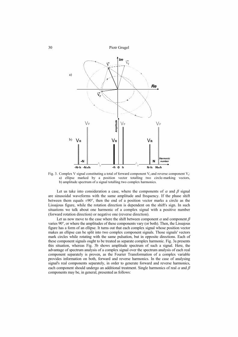
Fig. 3. Complex V signal constituting a total of forward component Vf and reverse component Vr:

a) ellipse marked by a position vector totalling two circle-marking vectors, b) amplitude spectrum of a signal totalling two complex harmonics.

Let us take into consideration a case, where the components of α and β signal

are sinusoidal waveforms with the same amplitude and frequency. If the phase shift between them equals ±90°, then the end of a position vector marks a circle as the Lissajous figure, while the rotation direction is dependent on the shift's sign. In such situations we talk about one harmonic of a complex signal with a positive number (forward rotation direction) or negative one (reverse direction).

Let us now move to the case where the shift between component α and component β varies 90°, or where the amplitudes of these components vary (or both). Then, the Lissajous figure has a form of an ellipse. It turns out that each complex signal whose position vector makes an ellipse can be split into two complex component signals. Those signals' vectors mark circles while rotating with the same pulsation, but in opposite directions. Each of these component signals ought to be treated as separate complex harmonic. Fig. 3a presents this situation, whereas Fig. 3b shows amplitude spectrum of such a signal. Here, the advantage of spectrum analysis of a complex signal over the spectrum analysis of each real component separately is proven, as the Fourier Transformation of a complex variable provides information on both, forward and reverse harmonics. In the case of analysing signal's real components separately, in order to generate forward and reverse harmonics, each component should undergo an additional treatment. Single harmonics of real α and β components may be, in general, presented as follows:

a)

b)

The use of complex sliding window Discrete Fourier Transformation... 31

( ) ( )( ) ( )

+Θ=Θ+Θ=Θ

ββ

αα

ψβψα

sinsin

XX

. (5)

(6)

Since rotating vector that marks an ellipse is a total of two vectors rotating in opposite directions that mark circles, each coordinate α and β components of the vector constitute a total of two sinusoidal waveforms. The former represents Cartesian components of forward harmonic, whereas the latter stands for a reverse one.

Using the theorem that each sinusoidal waveform with X amplitude and ψ phase can be composed of the sum of waveforms not shifted in phase (both sinusoidal and cosinusoidal), with amplitudes A and B respectively, the following formula appears:

( ) Θ+Θ=+Θ cossinsin BAX ψ . (7)

Relating (7) to (5) and (6), α and β cartesian components of forward and reverse harmonic are determined. Assuming limiting the solutions' set (7) to the case where A > 0 and B >0, the following system of equations is obtained:

=

+=

ABarctg

BAX

ψ

22

.

(8)

(9)

These are additional, very time-consuming calculations that a computation unit would have to conduct in the case of separate analysis of α and β real components with a view to distinguishing forward and reverse harmonics out of the complex signal.

Fig. 3b illustrates h-numbered band with Vf amplitude (forward component) and -h–numbered band with Vr amplitude (reverse component). The remaining bands are created in the result of aliasing, which cannot be avoided while operating on discrete series. The bands are called "aliases", as they represent frequency components which, in reality, do not exist in the investigated signal [1]. Working on N sequence of samples in a period, h-numbered band will additionally appear in a place of each harmonic

kNhhalias += , (10) where:

k – any integer number.

The phenomenon of aliasing cannot be eliminated during operating on quasi-continuous domain. It is very onerous, as in <-N÷N> bandwidth, according to (10), one is not able to distinguish harmonic value h from -N+h, or -h from N-h. What can be done is to limit the bandwidth of the analysed spectrum or choose an appropriate number of input samples by selecting the sampling frequency.

Taking into account that a harmonic number equalling H is analysed, M amount of bands is expected, where

12 += HM . (11)

Multiplication by two results from the fact that for a certain pulsation a vector can rotate both in forward and reverse way. Thus, it has to be considered as two separate harmonics. Yet, adding one results from the possibility of constant component's existence, which should also be analysed. The amount of samples needs to be twice as big as the number of analysed bands

32 Piotr Grugel

2N M= . (12)

Then, it is certain that no band from the positive bandwidth will appear in a negative part. One should bear in mind, however, that basing on (10), the components with frequencies higher than sampling frequency may come into being. Still, in practice, while analysing several dozen of current and voltage harmonics, the harmonics lying beyond the researched bandwidth are of insignificant value when compared to those within the bandwidth.

Through simulation, the spectrum of current's position vector in the circut presented in Fig. 2 has been researched. Fig. 4 shows the amplitudes and phases of separate current harmonics in the steady state. The results shown on the graphs prove that there are no even harmonics or harmonics with third multiple in the circut being researched [2, 3, 4]. The forward component of the first harmonic is significant (3,7A). At the same time the value of the fifth harmonic's reverse component (1,9A) is relatively high.

a)

b)

Fig. 4. The spectrum of current intaken by a six-pulse RL-loaded rectifier with a filtering

capacitor in DC circuit: a) amplitude spectrum, b) phase spectrum

The use of complex sliding window Discrete Fourier Transformation... 33

According to standards, in the case of determining THD factor for current, the analysis ought to include harmonic's measurement up to 40th number. In the results this number has been narrowed down to 20 in order to avoid darkening the picture with such a big amount of bands (40 complex harmonics give, according to (11), 81 bands). 3. COMPLEX SLIDING WINDOW DISCRETE FOURIER

TRANSFORMATION

In classic understanding, the implementation of DFT is based on collecting N number of signal's samples (which constitute the period of fundamental harmonic), then, the sequence of calculations based on (1) is conducted on these samples' set for each m harmonic that is of interest. After having conducted all necessary calculations, N sequence of samples is collected again and the whole procedure is repeated. This solution, however, has two major disadvantages. First of them is a computation unit's uneven loading, as all the calculations have to be performed in a short time (between collecting the last sample of one calculations' series and the first sample of the next series). The other disadvantage is obtaining calculations' results only after having collected the last sample in the period of fundamental harmonic. In the case where the harmonic analysis is used for implementation of a selective active filtration [7], the information about higher harmonics' appearence might already be out-of-date at the very moment of its obtainment. In such situation, the test on reactions on transition states turns out to be pointless.

The effects of the first inconvenience can be lessened by using the FFT algorithm, which leads to the limitation of computation unit's loading [1]. That, in turn, requires undergoing extra operations, such as additional actions in the number of input samples' selection, taking actions on the windows to limit spectral leakage, etc. Still, the problem of processor's uneven loading can be entirely eliminated by using double buffering of collected samples. In this case, the samples of a present waveform to one buffer are collected, at the same time, the calculations are being done on the other one, where the samples from a previous period are stored. However, such a solution increases disadvantageous lags in obtaining up-to date results.

The useful feature of DFT is the fact that it does not matter from which point in the periodic waveform's analysis is begun. What does matter is analysing as many successive samples as constitute one period of fundamental harmonic [1]. The amplitude spectrum for a given periodic waveform will always be the same, no matter the phase of signal's cutaway in the buffer (window) of samples constituting one period. The phase spectrum, however, depending on the analysed waveform's phase, will show, for each harmonic, a shift proportional to the relation of samples's number on which the window has been shifted to the number of samples constituting a period of a given harmonic. This can be written as follows:

nNm

m πϕ 2= , (13)

where: φm – stands for a phase shift of m-numbered harmonic, m – harmonic number for which a shift is calculated, N – number of samples constituting fundamental harmonic, n – number of samples on which the window's content has been shifted.

34 Piotr Grugel

Thus, stating that the buffer in which the input samples are stored constitutes the window the content of which is shifted on the analysed waveform on every new sample (the oldest sample in the window is displaced by new one's insertion) and not every N–samples (first harmonic's period) and that, every such step, the content is spectrum-analysed using DFT, then such an analysis is called “Sliding Window Discrete Fourier Transformation” (SDFT).

In the easiest way, Sliding Window can be pictured as a queue buffer. Still, it can also be realised as a ring buffer (such a solution has been put into practice in the investigated circuit). Owing to that, the phase spectrum is made independent from (13).

Fig. 5. Slipping the data in to the sliding window; the situation at t = 5 ms from the beginning of

slipping-in. The SDFT algorithm is of quasi-continuous type, thus, it returns information

concerning any change in a signal after each sampling. This feature makes it advantageous over typical DFT algorithm. However, one needs to be careful while interpreting the spectrum obtained in this way, as some changes taking place in the waveform are not periodic. Furthermore, only after a period of time equalling the width of a sliding window (which is the time equalling a period of fundamental harmonic) can changes connected with slipping in new harmonics to the signal be correctly interpreted.

The use of complex sliding window Discrete Fourier Transformation... 35

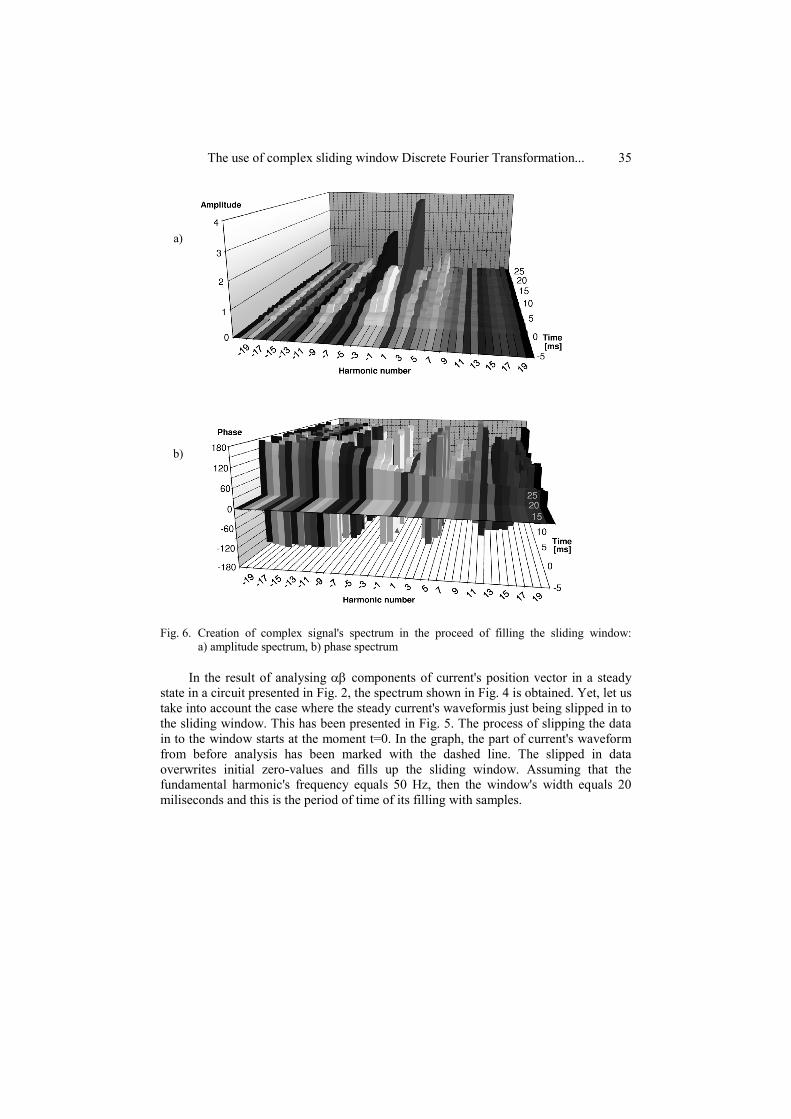
Fig. 6. Creation of complex signal's spectrum in the proceed of filling the sliding window: a) amplitude spectrum, b) phase spectrum

In the result of analysing αβ components of current's position vector in a steady state in a circuit presented in Fig. 2, the spectrum shown in Fig. 4 is obtained. Yet, let us take into account the case where the steady current's waveformis just being slipped in to the sliding window. This has been presented in Fig. 5. The process of slipping the data in to the window starts at the moment t=0. In the graph, the part of current's waveform from before analysis has been marked with the dashed line. The slipped in data overwrites initial zero-values and fills up the sliding window. Assuming that the fundamental harmonic's frequency equals 50 Hz, then the window's width equals 20 miliseconds and this is the period of time of its filling with samples.

a)

b)

36 Piotr Grugel

Fig. 7. Creation of the first harmonic of current's position vector in the process of filling

the sliding window: a) amplitude’s value, b) phase value The process of spectrum's creation is shown in Fig. 6. The window was filled with initial zero-values at the moment of its creation in digital memory. That is why before filling the window with samples' values, spectrum's bands picture zero-values of both amplitudes and phases of all harmonics. At the agreed moment of t=0, the process of filling the window with the samples' values that project the investigated complex signal began. The amplitude spectrum's bands change their heights at time and they are fixed at correct values after 20 miliseconds. In the result, the spectrum's picture shown in Fig. 4a is obtained. One should pay attention to the fact that the harmonic's bands which, in reality, do not exist in a waveform, present non-zero amplitudes' values before the spectrum's determining. Phase spectrum can be presented in a similar way. Here, the bands are established on the correct angle's values after the period of time equalling the window's width. However, the changes of band's values of phase spectrum are more violent than the amplitude spectrum's ones. Additionally, the higher-numbered harmonic they concern, the more intensive these changes are.

Fig. 7 presents the course of creating the amplitude and phase of only the first harmonic's waveform. As far as the amplitude is established in a mellow way, the phase at the moment of slipping in the first sample to the window discrete reaches the value

a)

b)

The use of complex sliding window Discrete Fourier Transformation... 37

of 87,8°. During the insertion of next samples the value oscillates reaching the extreme values of 55°, 90° and 77° successively. Only after having entirely filled the window, can one state that the phase is determined at the value of 90° and the amplitude at 3,7A.

4. IMPLEMENTATION OF THE COMPLEX VARIABLE'S SDFT AND THE PROPOSITION OF ITS ACCELERATING

As it has been mentioned before, one of DFT's disadvantages is big and uneven

loading of a computation unit with a great amount of calculations. Such loading takes place after each filling the buffer with the samples of an investigated waveform. Two buffers can be used in order to eliminate this phenomenon. Then, the former is filled with up-to-date samples, whereas the latter stores the samples from a previous signal and the calculations are performed on this buffer. At the same time, samples are collected to the first buffer. Such a solution decreases the loading's irregularity of a computation unit and makes the use of a cheaper, less efficient microprocessor possible. However, it delays appearing up-to-date calculations' results.

The SDFT algorithm updates the data concerning the whole spectrum after each new sample's collection. However, each conduction of calculations' cycle based on (1) would lead to loading a computation unit N times more than in the case of classic DFT implementation (which is already very time-consuming). Nevertheless, it turns out that there is no need to conduct such a big amount of mathematical calculations. In accordance with (1), m–number harmonic's determining resolves to counting up the sum of products of each x(n) sample's value in one signal's period with the following term:

)/2sin()/2cos( NnmjNnm ππ − . (14)

Memorising the up-to-date values of all M harmonics and values of all N products of

( ) ( ))/2sin()/2cos( NnmjNnmnx ππ −⋅ , (15)

one can, after each sample's collection, calculate a new value of m-number harmonic as its up-to-date value reduced by (15), calculated for the oldest sample in the window, and increased by the same (15), calculated for a newly collected sample. After having conducted all those actions, the oldest sample in the window is replaced by a newly calculated one.

According to the example above, calculating each harmonic's value after collecting a new sample resolves to one multiplication (15), one subtraction and one addition. Still, one has to bear in mind the fact that the term (14) appears in each multiplication that requires additional trigonometrical operations, and in the case of complex variable's SDFT, basing on (4), each multiplication requires counting up four trigonometrical products.

38 Piotr Grugel

Fig. 8. Algorithm presenting implementation of Complex SDFT The complete algorithm enabling implementation of Complex SDFT

for H harmonics, both forward and reverse, has been presented in Fig. 8. During the analysis of mathematical operations that are crucial in SDFT

algorithm's realisation, it is easy to observe that what is the most time-consuming for a processor is trigonometrical calculations specified in (14). As there are no low-level processor's commands that conduct trigonometrical calculations, in reality, high-level programming languages use algorithms that approximate these functions' results. The approximation of sine and cosine functions that is most often used is their Taylor series expansion.

∑

∑∞

=

∞

=

+

−+−=−=

−+−=+

−=

0

422

53

0

12

...!4!2

1)!2(

)1()cos(

...!5!3)!12(

)1()sin(

n

nn

n

nn

xxn

xx

xxxnxx

.

(16)

(17)

In reality, a computation unit does not calculate an infinite sequence, the number of n polynomical depends on the implementation of used programming language and reaches, in practice, several dozens iterations. This is of adequate precision for the majority of algorithms. However, counting up the value of a given angle's sine and cosine remains very time-consuming for every microprocessor, especially for the one not equipped with Floating-Point Unit (FPU).

The use of complex sliding window Discrete Fourier Transformation... 39

Fig. 9. Algorithm presenting the implementation of Complex SDFT with the use of arrayed values of trigonometric functions

Since one certain value of sine or cosine function corresponds with each angle's value, it can be of help to store some of these values on an array and use them when needed (instead of calculating them for each time). The disadvantage of this solution, however, is increasing the application's demand for memory in which the array is stored. Another inconvenience may be unsatisfactory accuracy of this solution. For example, storing 360 values with a discrete by one degree, there is no possibility to determine an angle's function with the value of a degree's fraction. Certainly, it is possible to increase resolution by arraying the function's values by, for instance, 1/10 degree. This will make the results more accurate, but increase the demand for memory by ten times.

40 Piotr Grugel

Looking at the relations (1) and (4), one can notice that the angle's values appearing under trigonometric functions are not accidental. The indexes n and m are integer variables, the values of which comprise in ranges <0, N-1> and <0, M-1> respectively. N value, according to (12) and (11), is constant for the agreed number of analysed H harmonics. Thus, the amount of all possible angles for which sine and cosine values ought to be calculated, is limited to N×M. For instance, for H=40, according to (11) and (12), N×M=13122. Another advantage of this solution is the fact that the values organised in the array in such a way guarantee the same accuracy as their each-time calculating.

The algorithm enabling the above method's implementation has been shown in Fig. 9.

After having implemented the algorithm with the arrayed values of trigonometric functions in a physical circuit based on microcontroller devoid of FPU, its efficiency is over 100 times higher comparing to the version with calculating values for each time. In this case, the demand for memory in respect to the price of a faster processor proves to be of insignificant costs. That is why, if in realised application, SDFT algorithm is the most time-consuming for a computation unit, equipping the application with a cheaper processor and bigger memory turns out to be a more economic solution.

5. SUMMARY

Presented algorithm of current's spectrum analysis with the use of complex variable's Sliding Window Discrete Fourier Transformation (SDFT) can be implemented in the real time systems. The obtained results of spectrum analysis can be used as input data of the active filtration's algorithm. This is the subject of further research carried out in the Department of Power Electronics and Control at University of Technology and Life Sciences in Bydgoszcz.

The algorithm has been developed at University of Technology and Life Sciences in Bydgoszcz with the use of C++ programming language and simulated at Gdynia Maritime University with PSIM v7 simulation environment. BIBLIOGRAPHY [1] Lyons R.G., 2003. Wprowadzenie do cyfrowego przetwarzania sygnałów. WKŁ,

Warszawa. [2] Piróg S., 2006. Układy o komutacji sieciowej i o komutacji twardej. AGH,

Kraków. [3] Czarnecki L.S., 2005. Moce w obwodach elektrycznych z niesinusoidalnymi

przebiegami prądów i napięć. Oficyna Wydawnicza PW, Warszawa. [4] Nowak M., Barlik R., 1998. Poradnik inżyniera energoelektronika. WNT,

Warszawa. [5] Akagi H., Edson H. W., Mauricio A., 2007. Instantaneous power theory and

applications to power conditioning. IEEE Press. [6] Strzelecki R., Benysek G., Noculak A., 2003. Wykorzystanie urządzeń energo-

elektronicznych w systemie elektroenergetycznym. Przegląd Elektrotechniczny 2.

The use of complex sliding window Discrete Fourier Transformation... 41

[7] Mućko J., 2008. Jednofazowy filtr hybrydowy wybranej harmonicznej. Materiały konferencyjne Modelowanie i Symulacja MiS-5.

[8] Orłowska-Kowalska T., 2003. Bezczujnikowe układy napędowe z silnikami indukcyjnymi. Oficyna Wydawnicza PW, Wrocław.

WYKORZYSTANIE DYSKRETNEJ TRANSFORMATY FOURIERA ZMIENNEJ ZESPOLONEJ ZE ŚLIZGAJĄCYM OKNEM DO ANALIZY

ODKSZTAŁCEŃ PRĄDÓW I NAPIĘĆ W UKŁADACH TRÓJFAZOWYCH

Streszczenie

Artykuł przedstawia aspekty wektorowej analizy odkształconych przebiegów prądów i napięć w układach trójfazowych pod kątem zawartości wyższych harmonicznych. Praca zawiera również wyniki analizy harmonicznej wektora prądu opartej o transformatę Fouriera zmiennej zespolonej ze ślizgającym oknem (complex SDFT) uzyskane na drodze symulacji oraz propozycję przyspieszenia algorytmu SDFT w celu ułatwienia jego implementacji w układach pracujących w czasie rzeczywistym.

Słowa kluczowe: Dyskretna Transformata Fouriera zmiennej zespolonej ze ślizga-jącym oknem, selektywna filtracja aktywna, analiza widmowa wektora wodzącego, odkształcone przebiegi prądu i napięcia