Effects of surrounding stimulus properties on color...

Effects of surrounding stimulus properties oncolor constancy based on luminance balanceTAKUMA MORIMOTO,1,* KAZUHO FUKUDA,2 AND KEIJI UCHIKAWA1

1Department of Information Processing, Tokyo Institute of Technology, 226-8503 Yokohama, Japan2Department of Information Design, Kogakuin University, 163-8677 Tokyo, Japan*Corresponding author: [email protected]

Received 30 September 2015; revised 1 January 2016; accepted 1 January 2016; posted 5 January 2016 (Doc. ID 250930);published 17 February 2016

The visual system needs to discount the influence of an illuminant to achieve color constancy. Uchikawa et al.[J. Opt. Soc. Am. A29, A133 (2012)] showed that the luminance-balance change of surfaces in a scene contributesto illuminant estimation; however, its effect was substantially less than the chromaticity change. We conduct threeexperiments to reinforce the previous findings and investigate possible factors that can influence the effect ofluminance balance. Experimental results replicate the previous finding; i.e., luminance balance makes a small,but significant, contribution to illuminant estimation. We find that stimulus dimensionality affects neither thedegree of color constancy nor the effect of luminance balance. Unlike chromaticity-based color constancy, chro-matic variation does not influence the effect of luminance balance. It is shown that luminance-balance-basedestimation of an illuminant performs better for scenes with reddish or bluish surfaces. This suggests that thevisual system exploits the optimal color distribution for illuminant estimation [J. Opt. Soc. Am. A 29, A133(2012)]. © 2016 Optical Society of America

OCIS codes: (330.1690) Color; (330.1720) Color vision.

http://dx.doi.org/10.1364/JOSAA.33.00A214

1. INTRODUCTION

When an illuminant changes, the chromaticity and luminanceof a surface in a scene accordingly change. However, our per-ception of surface color does not change significantly. This vis-ual property, which is known as color constancy, allows us toidentify objects under different illuminants. To achieve colorconstancy, the visual system needs to discount the influenceof the illuminant. However, such a subtraction is mathemati-cally impossible because light entering our eyes is the product ofthe surface spectral reflectance and the illuminant spectral com-position. Therefore, in some sense, the visual system needs toestimate the illuminant by exploiting various cues in the scene.Although there has been a substantial amount of research intocolor constancy, as recently summarized in review papers [1–3],its mechanism remains unclear.

Many potential algorithms have been proposed. One of thesimplest solutions is retinal adaptation, known as von Kriesadaptation [4]. A similar cone-based mechanism is Ives trans-formation [5], which considers cone signals globally across theretina, whereas von Kries adaptation acts locally. Althoughthese low-level processes often provide sufficient cues forcolor constancy, the contributions of the higher-level visualprocess have also been reported [6]. Therefore, it is generallyacknowledged that color constancy is not a specific level

process; several types of visual processes appear to underlie itin complex ways.

Another common approach to color constancy is to charac-terize the distribution of colors in a natural scene under variousilluminants. Foster and Nascimento [7] pointed out that anilluminant change does not largely affect the spatial cone ratio;therefore, the visual system can use the invariant signal regard-less of illuminant change, which might provide the basis ofcolor constancy. Interestingly, unlike many other color con-stancy algorithms, this method allows the visual system to dis-tinguish between the material change and the illuminantchange without illuminant estimation.

It is known that brighter surfaces are better cues to estimatethe illuminant than darker surfaces [8]. In its extreme form, aspecular highlight would be particularly helpful because theydirectly convey an illuminant to the eye [9]. However,Fukuda and Uchikawa [10] found that colors appearing inthe aperture-color mode do not significantly contribute tothe degree of color constancy, suggesting that the visual systemprimarily exploits the colors in the surface-color appearance toestimate an illuminant.

In addition to these local cues interspersing in the scene,spatially global cues also seem to be reliable because the illu-minant affects surfaces in a wide range of the scene. It is well

A214 Vol. 33, No. 3 / March 2016 / Journal of the Optical Society of America A Research Article

1084-7529/16/03A214-14$15/0$15.00 © 2016 Optical Society of America

http://dx.doi.org/10.1364/JOSAA.33.00A214

known that simply taking a spatial average of scene chromatic-ity often provides a sufficient cue to estimate the illuminantunder a constraint of the gray world hypothesis [11].However, this method fails when the gray world hypothesisfails, and it is actually common that the scene is not gray[12]. As this acknowledged model implies, there has been ahistorical bias toward exploiting chromaticity to estimate theilluminant even though an illuminant change should also affectthe luminance of surfaces in a scene.

One of the long-standing mysteries in the color constancyfield has been how the visual system distinguishes a reddishscene under a neutral illuminant from a neutral scene undera reddish illuminant when both produce exactly same meanchromaticity. This problem was sharply focused on by Golzand MacLeod [13], who showed that surfaces with higher red-ness tend to have higher luminances under a reddish illumi-nant, resulting in a positive correlation between redness andluminance. They empirically showed that the visual systemcan exploit this correlation between luminance and rednessto solve the ambiguity of mean chromaticity. The importantimplication shown by their study is that the luminance playsa significant role in illuminant estimation.

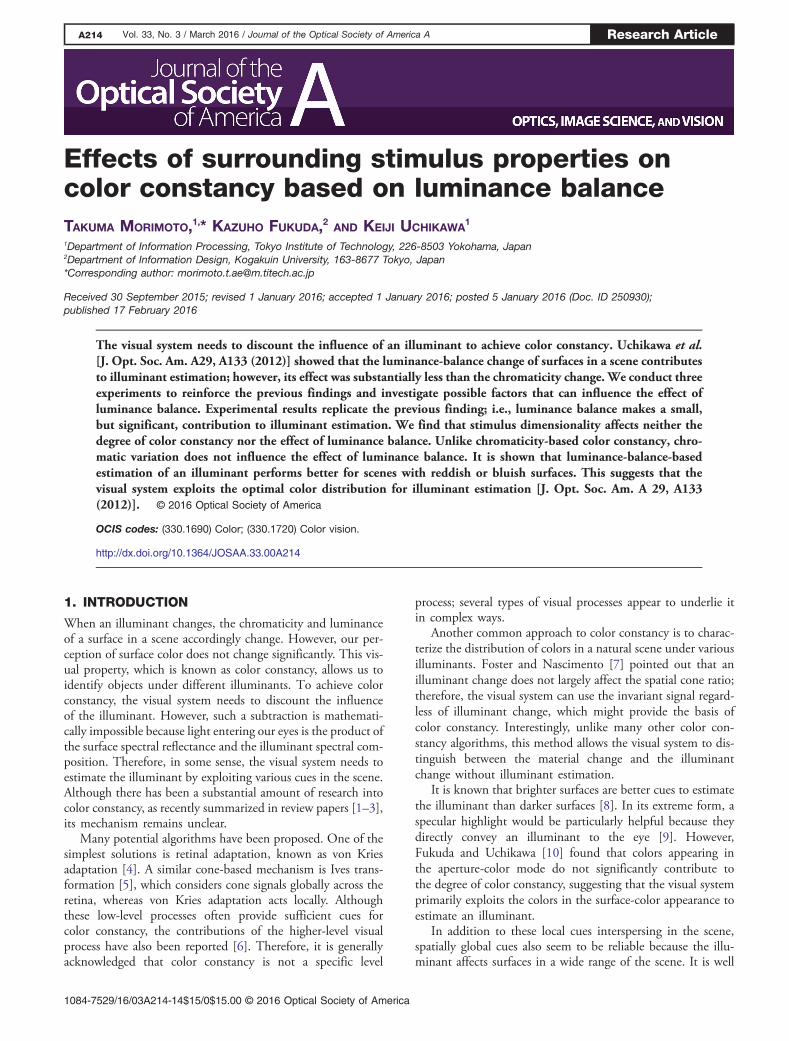
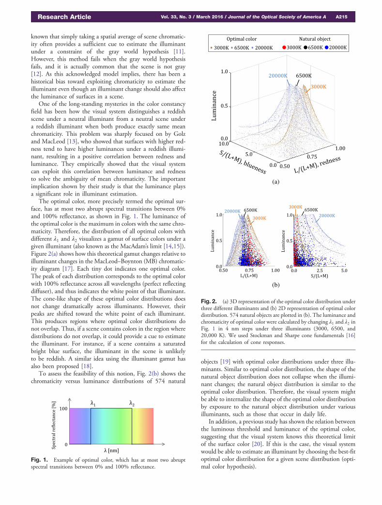
The optimal color, more precisely termed the optimal sur-face, has at most two abrupt spectral transitions between 0%and 100% reflectance, as shown in Fig. 1. The luminance ofthe optimal color is the maximum in colors with the same chro-maticity. Therefore, the distribution of all optimal colors withdifferent λ1 and λ2 visualizes a gamut of surface colors under agiven illuminant (also known as the MacAdam’s limit [14,15]).Figure 2(a) shows how this theoretical gamut changes relative toilluminant changes in the MacLeod–Boynton (MB) chromatic-ity diagram [17]. Each tiny dot indicates one optimal color.The peak of each distribution corresponds to the optimal colorwith 100% reflectance across all wavelengths (perfect reflectingdiffuser), and thus indicates the white point of that illuminant.The cone-like shape of these optimal color distributions doesnot change dramatically across illuminants. However, theirpeaks are shifted toward the white point of each illuminant.This produces regions where optimal color distributions donot overlap. Thus, if a scene contains colors in the region wheredistributions do not overlap, it could provide a cue to estimatethe illuminant. For instance, if a scene contains a saturatedbright blue surface, the illuminant in the scene is unlikelyto be reddish. A similar idea using the illuminant gamut hasalso been proposed [18].

To assess the feasibility of this notion, Fig. 2(b) shows thechromaticity versus luminance distributions of 574 natural

objects [19] with optimal color distributions under three illu-minants. Similar to optimal color distribution, the shape of thenatural object distribution does not collapse when the illumi-nant changes; the natural object distribution is similar to theoptimal color distribution. Therefore, the visual system mightbe able to internalize the shape of the optimal color distributionby exposure to the natural object distribution under variousilluminants, such as those that occur in daily life.

In addition, a previous study has shown the relation betweenthe luminous threshold and luminance of the optimal color,suggesting that the visual system knows this theoretical limitof the surface color [20]. If this is the case, the visual systemwould be able to estimate an illuminant by choosing the best-fitoptimal color distribution for a given scene distribution (opti-mal color hypothesis).

Fig. 1. Example of optimal color, which has at most two abruptspectral transitions between 0% and 100% reflectance.

(a)

(b)

Fig. 2. (a) 3D representation of the optimal color distribution underthree different illuminants and (b) 2D representation of optimal colordistribution. 574 natural objects are plotted in (b). The luminance andchromaticity of optimal color were calculated by changing λ1 and λ2 inFig. 1 in 4 nm steps under three illuminants (3000, 6500, and20,000 K). We used Stockman and Sharpe cone fundamentals [16]for the calculation of cone responses.

Research Article Vol. 33, No. 3 / March 2016 / Journal of the Optical Society of America A A215

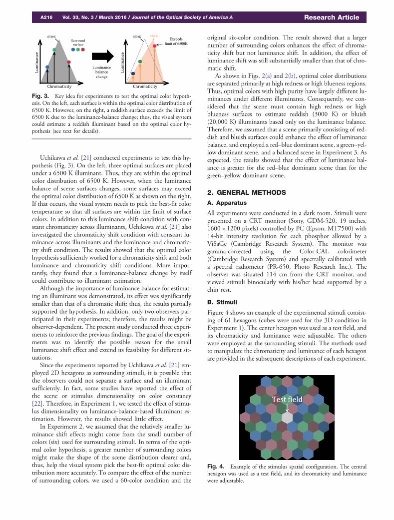
Uchikawa et al. [21] conducted experiments to test this hy-pothesis (Fig. 3). On the left, three optimal surfaces are placedunder a 6500 K illuminant. Thus, they are within the optimalcolor distribution of 6500 K. However, when the luminancebalance of scene surfaces changes, some surfaces may exceedthe optimal color distribution of 6500 K as shown on the right.If that occurs, the visual system needs to pick the best-fit colortemperature so that all surfaces are within the limit of surfacecolors. In addition to this luminance shift condition with con-stant chromaticity across illuminants, Uchikawa et al. [21] alsoinvestigated the chromaticity shift condition with constant lu-minance across illuminants and the luminance and chromatic-ity shift condition. The results showed that the optimal colorhypothesis sufficiently worked for a chromaticity shift and bothluminance and chromaticity shift conditions. More impor-tantly, they found that a luminance-balance change by itselfcould contribute to illuminant estimation.

Although the importance of luminance balance for estimat-ing an illuminant was demonstrated, its effect was significantlysmaller than that of a chromatic shift; thus, the results partiallysupported the hypothesis. In addition, only two observers par-ticipated in their experiments; therefore, the results might beobserver-dependent. The present study conducted three experi-ments to reinforce the previous findings. The goal of the experi-ments was to identify the possible reason for the smallluminance shift effect and extend its feasibility for different sit-uations.

Since the experiments reported by Uchikawa et al. [21] em-ployed 2D hexagons as surrounding stimuli, it is possible thatthe observers could not separate a surface and an illuminantsufficiently. In fact, some studies have reported the effect ofthe scene or stimulus dimensionality on color constancy[22]. Therefore, in Experiment 1, we tested the effect of stimu-lus dimensionality on luminance-balance-based illuminant es-timation. However, the results showed little effect.

In Experiment 2, we assumed that the relatively smaller lu-minance shift effects might come from the small number ofcolors (six) used for surrounding stimuli. In terms of the opti-mal color hypothesis, a greater number of surrounding colorsmight make the shape of the scene distribution clearer and,thus, help the visual system pick the best-fit optimal color dis-tribution more accurately. To compare the effect of the numberof surrounding colors, we used a 60-color condition and the

original six-color condition. The result showed that a largernumber of surrounding colors enhances the effect of chroma-ticity shift but not luminance shift. In addition, the effect ofluminance shift was still substantially smaller than that of chro-matic shift.

As shown in Figs. 2(a) and 2(b), optimal color distributionsare separated primarily at high redness or high blueness regions.Thus, optimal colors with high purity have largely different lu-minances under different illuminants. Consequently, we con-sidered that the scene must contain high redness or highblueness surfaces to estimate reddish (3000 K) or bluish(20,000 K) illuminants based only on the luminance balance.Therefore, we assumed that a scene primarily consisting of red-dish and bluish surfaces could enhance the effect of luminancebalance, and employed a red–blue dominant scene, a green–yel-low dominant scene, and a balanced scene in Experiment 3. Asexpected, the results showed that the effect of luminance bal-ance is greater for the red–blue dominant scene than for thegreen–yellow dominant scene.

2. GENERAL METHODS

A. Apparatus

All experiments were conducted in a dark room. Stimuli werepresented on a CRT monitor (Sony, GDM-520, 19 inches,1600 × 1200 pixels) controlled by PC (Epson, MT7500) with14-bit intensity resolution for each phosphor allowed by aViSaGe (Cambridge Research System). The monitor wasgamma-corrected using the Color-CAL colorimeter(Cambridge Research System) and spectrally calibrated witha spectral radiometer (PR-650, Photo Research Inc.). Theobserver was situated 114 cm from the CRT monitor, andviewed stimuli binocularly with his/her head supported by achin rest.

B. Stimuli

Figure 4 shows an example of the experimental stimuli consist-ing of 61 hexagons (cubes were used for the 3D condition inExperiment 1). The center hexagon was used as a test field, andits chromaticity and luminance were adjustable. The otherswere employed as the surrounding stimuli. The methods usedto manipulate the chromaticity and luminance of each hexagonare provided in the subsequent descriptions of each experiment.

Fig. 3. Key idea for experiments to test the optimal color hypoth-esis. On the left, each surface is within the optimal color distribution of6500 K. However, on the right, a reddish surface exceeds the limit of6500 K due to the luminance-balance change; thus, the visual systemcould estimate a reddish illuminant based on the optimal color hy-pothesis (see text for details).

Fig. 4. Example of the stimulus spatial configuration. The centralhexagon was used as a test field, and its chromaticity and luminancewere adjustable.


Hexagons were 2° diagonally, and the whole stimulus conse-quently subtended 15.6° by 14.0° �w × h�.C. Observers

Four observers participated in all experiments. Three maleobservers were 20–29 years of age, and one female observer(HH) was 30–39 years of age. All observers had normal colorvision assessed by Ishihara Pseudoisochromatic Plate tests. TMwas an author.

D. Procedure

The observer was instructed to adjust both the chromaticityand luminance of the test field so that it appeared as a full-whitepaper under a test illuminant (paper-match criterion [23]) witha track ball and a keypad. The chromaticity adjustment wasperformed two-dimensionally on the MB chromaticity dia-gram. For all experiments, we defined the chromaticity and lu-minance of the test field selected as a full-white paper by theobserver as an estimated illuminant chromaticity and intensity,respectively.

Prior to starting the first trial, the observer first adapted to anequal energy white light (33.0 cd∕m2) that covered the full dis-playable area of the CRT monitor for 2 min. Both the initialchromaticity and luminance of the test field were chosen ran-domly from a possible range for each trial. After satisfactoryadjustments without time limitations, the observer recordedtheir final choice. One block consisted of five successive rep-etitions without inter-trial interval. In the same block, the samesurrounding stimuli but different spatial arrangements werepresented. The observer readapted to the equal energy whitefor 30 s between blocks. One session comprised 18 blocksin Experiments 1 and 3 and 17 blocks in Experiment 2.The order of the conditions was fully randomized within asession. The observer performed four sessions resulting in20 repetitions for each condition.

3. EXPERIMENT 1

A. Surrounding Stimuli

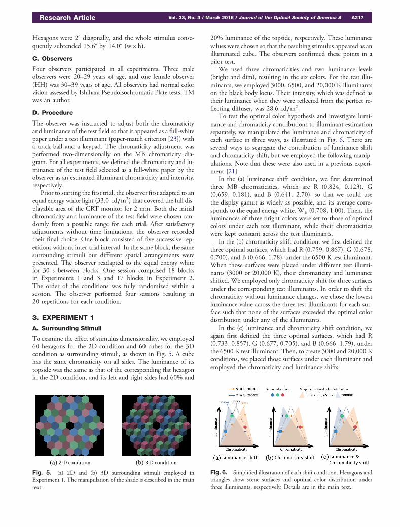
To examine the effect of stimulus dimensionality, we employed60 hexagons for the 2D condition and 60 cubes for the 3Dcondition as surrounding stimuli, as shown in Fig. 5. A cubehas the same chromaticity on all sides. The luminance of itstopside was the same as that of the corresponding flat hexagonin the 2D condition, and its left and right sides had 60% and

20% luminance of the topside, respectively. These luminancevalues were chosen so that the resulting stimulus appeared as anilluminated cube. The observers confirmed these points in apilot test.

We used three chromaticities and two luminance levels(bright and dim), resulting in the six colors. For the test illu-minants, we employed 3000, 6500, and 20,000 K illuminantson the black body locus. Their intensity, which was defined astheir luminance when they were reflected from the perfect re-flecting diffuser, was 28.6 cd∕m2.

To test the optimal color hypothesis and investigate lumi-nance and chromaticity contributions to illuminant estimationseparately, we manipulated the luminance and chromaticity ofeach surface in three ways, as illustrated in Fig. 6. There areseveral ways to segregate the contribution of luminance shiftand chromaticity shift, but we employed the following manip-ulations. Note that these were also used in a previous experi-ment [21].

In the (a) luminance shift condition, we first determinedthree MB chromaticities, which are R (0.824, 0.123), G(0.659, 0.181), and B (0.641, 2.70), so that we could usethe display gamut as widely as possible, and its average corre-sponds to the equal energy white,WE (0.708, 1.00). Then, theluminances of three bright colors were set to those of optimalcolors under each test illuminant, while their chromaticitieswere kept constant across the test illuminants.

In the (b) chromaticity shift condition, we first defined thethree optimal surfaces, which had R (0.759, 0.867), G (0.678,0.700), and B (0.666, 1.78), under the 6500 K test illuminant.When those surfaces were placed under different test illumi-nants (3000 or 20,000 K), their chromaticity and luminanceshifted. We employed only chromaticity shift for three surfacesunder the corresponding test illuminants. In order to shift thechromaticity without luminance changes, we chose the lowestluminance value across the three test illuminants for each sur-face such that none of the surfaces exceeded the optimal colordistribution under any of the illuminants.

In the (c) luminance and chromaticity shift condition, weagain first defined the three optimal surfaces, which had R(0.733, 0.857), G (0.677, 0.705), and B (0.666, 1.79), underthe 6500 K test illuminant. Then, to create 3000 and 20,000 Kconditions, we placed those surfaces under each illuminant andemployed the chromaticity and luminance shifts.

(a) (b)

Fig. 5. (a) 2D and (b) 3D surrounding stimuli employed inExperiment 1. The manipulation of the shade is described in the maintext.

Fig. 6. Simplified illustration of each shift condition. Hexagons andtriangles show scene surfaces and optimal color distribution underthree illuminants, respectively. Details are in the main text.


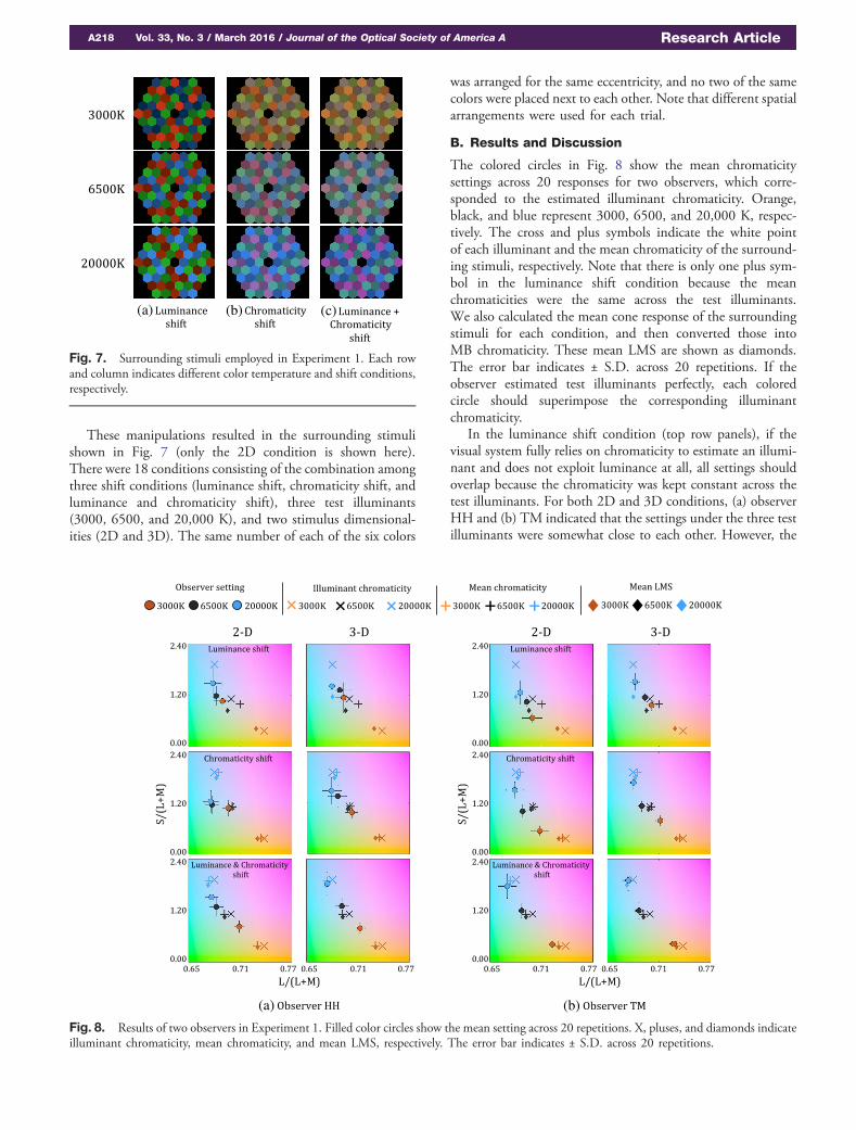
These manipulations resulted in the surrounding stimulishown in Fig. 7 (only the 2D condition is shown here).There were 18 conditions consisting of the combination amongthree shift conditions (luminance shift, chromaticity shift, andluminance and chromaticity shift), three test illuminants(3000, 6500, and 20,000 K), and two stimulus dimensional-ities (2D and 3D). The same number of each of the six colors

was arranged for the same eccentricity, and no two of the samecolors were placed next to each other. Note that different spatialarrangements were used for each trial.

B. Results and Discussion

The colored circles in Fig. 8 show the mean chromaticitysettings across 20 responses for two observers, which corre-sponded to the estimated illuminant chromaticity. Orange,black, and blue represent 3000, 6500, and 20,000 K, respec-tively. The cross and plus symbols indicate the white pointof each illuminant and the mean chromaticity of the surround-ing stimuli, respectively. Note that there is only one plus sym-bol in the luminance shift condition because the meanchromaticities were the same across the test illuminants.We also calculated the mean cone response of the surroundingstimuli for each condition, and then converted those intoMB chromaticity. These mean LMS are shown as diamonds.The error bar indicates ± S.D. across 20 repetitions. If theobserver estimated test illuminants perfectly, each coloredcircle should superimpose the corresponding illuminantchromaticity.

In the luminance shift condition (top row panels), if thevisual system fully relies on chromaticity to estimate an illumi-nant and does not exploit luminance at all, all settings shouldoverlap because the chromaticity was kept constant across thetest illuminants. For both 2D and 3D conditions, (a) observerHH and (b) TM indicated that the settings under the three testilluminants were somewhat close to each other. However, the

(a) (b) (c)

Fig. 7. Surrounding stimuli employed in Experiment 1. Each rowand column indicates different color temperature and shift conditions,respectively.

(a) (b)

Fig. 8. Results of two observers in Experiment 1. Filled color circles show the mean setting across 20 repetitions. X, pluses, and diamonds indicateilluminant chromaticity, mean chromaticity, and mean LMS, respectively. The error bar indicates ± S.D. across 20 repetitions.


settings under 3000 and 20,000 K shifted slightly toward thewhite point of the corresponding illuminant.

For (a) observer HH, for both 2D and 3D conditions,multiple comparisons with Bonferroni’s correction (significancelevel: 0.05) showed that the setting under 3000 Kwas separatedsignificantly from the settings under 6500 and 20,000 K in theredness direction. It was also shown that the setting under20,000 K was separated significantly from the settings under3000 and 6500 K in the blueness direction in the 2D condi-tion, but only from the setting under 3000 K in the 3D con-dition. For (b) observer TM, for both 2D and 3D conditions,settings under the three illuminants were separated significantlyin both the redness and blueness directions. Therefore,although the amounts of shifts were substantially smaller thanthe physical shift of the illuminant chromaticity, these resultsconfirm that the visual system seems to exploit the luminancebalance to estimate an illuminant to some extent.

In the chromaticity shift condition (middle row panels) inthe 2D condition for (a) observer HH, the settings under 6500and 20,000 K were clustered closely, but the setting under3000 K was distant from the settings under 6500 and20,000 K. The 3D condition appears to show somewhat betterestimations than the 2D condition. The (b) observer TMshowed better estimations than those observed in the lumi-nance shift condition in both 2D and 3D conditions.Therefore, as expected, the visual system was able to exploitchromaticity to estimate an illuminant even when the lumi-nance did not change across the test illuminants.

In the luminance and chromaticity shift condition (bottomrow panels), both observers’ estimated points of the illuminantsfor 3000 and 20,000 K shifted more than the other two shiftconditions for both the 2D and 3D conditions.

However, overall, the effect of stimulus dimensionality ap-pears small or nearly absent. The other two observers alsoshowed similar trends.

To quantify the relative amount of shift between the settingsunder 6500 and 3000 K or 20,000 K, we calculated a con-stancy index. However, to argue the amount of shift properly,it would be necessary to unify the scale of both axes in the MBchromaticity diagram. Thus, we divided both axes by the S.D.of the settings under 6500 K separately for each condition.Although the method to quantify the degree of color constancyremains controversial [1], we define it as Eq. (1) in the presentstudy:

CI � a∕b (1)

In Eq. (1), a indicates the distance between the observer settingunder 6500 K and either 3000 or 20,000 K, and b is thedistance between the illuminant chromaticity points. Higherconstancy index (CI) values indicate better color constancy.

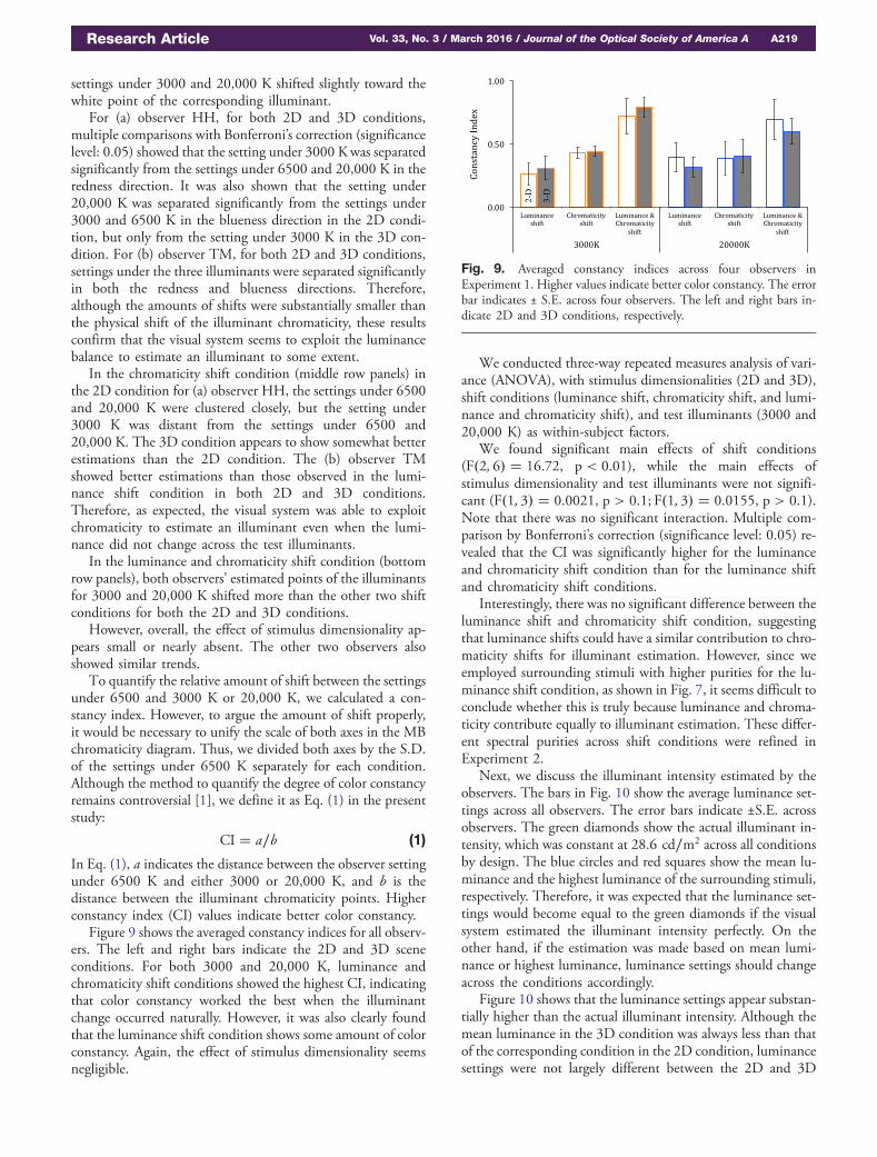
Figure 9 shows the averaged constancy indices for all observ-ers. The left and right bars indicate the 2D and 3D sceneconditions. For both 3000 and 20,000 K, luminance andchromaticity shift conditions showed the highest CI, indicatingthat color constancy worked the best when the illuminantchange occurred naturally. However, it was also clearly foundthat the luminance shift condition shows some amount of colorconstancy. Again, the effect of stimulus dimensionality seemsnegligible.

We conducted three-way repeated measures analysis of vari-ance (ANOVA), with stimulus dimensionalities (2D and 3D),shift conditions (luminance shift, chromaticity shift, and lumi-nance and chromaticity shift), and test illuminants (3000 and20,000 K) as within-subject factors.

We found significant main effects of shift conditions(F�2; 6� � 16.72, p < 0.01), while the main effects ofstimulus dimensionality and test illuminants were not signifi-cant (F�1; 3� � 0.0021, p > 0.1; F�1; 3� � 0.0155, p > 0.1).Note that there was no significant interaction. Multiple com-parison by Bonferroni’s correction (significance level: 0.05) re-vealed that the CI was significantly higher for the luminanceand chromaticity shift condition than for the luminance shiftand chromaticity shift conditions.

Interestingly, there was no significant difference between theluminance shift and chromaticity shift condition, suggestingthat luminance shifts could have a similar contribution to chro-maticity shifts for illuminant estimation. However, since weemployed surrounding stimuli with higher purities for the lu-minance shift condition, as shown in Fig. 7, it seems difficult toconclude whether this is truly because luminance and chroma-ticity contribute equally to illuminant estimation. These differ-ent spectral purities across shift conditions were refined inExperiment 2.

Next, we discuss the illuminant intensity estimated by theobservers. The bars in Fig. 10 show the average luminance set-tings across all observers. The error bars indicate ±S.E. acrossobservers. The green diamonds show the actual illuminant in-tensity, which was constant at 28.6 cd∕m2 across all conditionsby design. The blue circles and red squares show the mean lu-minance and the highest luminance of the surrounding stimuli,respectively. Therefore, it was expected that the luminance set-tings would become equal to the green diamonds if the visualsystem estimated the illuminant intensity perfectly. On theother hand, if the estimation was made based on mean lumi-nance or highest luminance, luminance settings should changeacross the conditions accordingly.

Figure 10 shows that the luminance settings appear substan-tially higher than the actual illuminant intensity. Although themean luminance in the 3D condition was always less than thatof the corresponding condition in the 2D condition, luminancesettings were not largely different between the 2D and 3D

Fig. 9. Averaged constancy indices across four observers inExperiment 1. Higher values indicate better color constancy. The errorbar indicates ± S.E. across four observers. The left and right bars in-dicate 2D and 3D conditions, respectively.


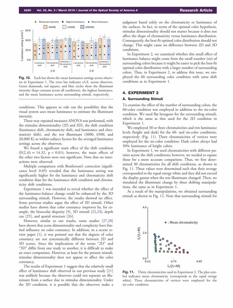
conditions. This appears to rule out the possibility that thevisual system uses mean luminance to estimate the illuminantintensity.

Three-way repeated measures ANOVAwas performed, withthe stimulus dimensionality (2D and 3D), the shift condition(luminance shift, chromaticity shift, and luminance and chro-maticity shift), and the test illuminant (3000, 6500, and20,000 K) as within-subject factors for the averaged luminancesettings across the observers.

We found a significant main effect of the shift condition(F�2; 6� � 14.32, p < 0.01); however, the main effects ofthe other two factors were not significant. Note that no inter-actions were observed.

Multiple comparison with Bonferroni’s correction (signifi-cance level: 0.05) revealed that the luminance setting wassignificantly higher for the luminance and chromaticity shiftcondition than for the luminance shift condition and chroma-ticity shift conditions.

Experiment 1 was intended to reveal whether the effect ofthe luminance-balance change could be enhanced by the 3Dsurrounding stimuli. However, the results showed no effect.Some previous studies argue the effect of 3D stimuli. Otherstudies have shown that color constancy improves by, for ex-ample, the binocular disparity [9], 3D stimuli [22,24], depthcue [25], and spatial structure [26].

However, similar to our results, some studies [27,28]have shown that scene dimensionality and complexity have lim-ited influence on color constancy. In addition, in a recent re-view paper [1], it was pointed out that the degrees of colorconstancy are not systematically different between 2D and3D scenes. Since the implications of the terms “2D” and“3D” differ from one study to another, it is difficult to makean exact comparison. However, at least for the present stimuli,stimulus dimensionality does not appear to affect the colorconstancy.

The results of Experiment 1 suggest that the relatively smalleffect of luminance shift observed in our previous study [21]was unlikely because the observers could not separate an illu-minant from a surface due to stimulus dimensionality. Underthe 3D condition, it is possible that the observers make a

judgment based solely on the chromaticity or luminance ofthe surfaces. In fact, in terms of the optimal color hypothesis,stimulus dimensionality should not matter because it does notaffect the shape of chromaticity versus luminance distribution.Consequently, the best-fit optimal color distribution should notchange. This might cause no difference between 2D and 3Dconditions.

In Experiment 2, we examined whether this small effect ofluminance balance might come from the small number (six) ofsurrounding colors because it might be easier to pick the best-fitoptimal color distribution with a larger number of surroundingcolors. Thus, in Experiment 2, to address this issue, we em-ployed the 60 surrounding color condition with same shiftconditions as in Experiment 1.

4. EXPERIMENT 2


To examine the effect of the number of surrounding colors, the60-color condition was employed in addition to the six-colorcondition. We used flat hexagons for the surrounding stimuli,which is the same as that used for the 2D condition inExperiment 1.

We employed 30 or three chromaticities and two luminancelevels (bright and dark) for the 60- and six-color conditions,respectively (Fig. 11). Three chromaticities of vertices wereemployed for the six-color condition. Dark colors always had50% luminance of bright colors.

In Experiment 1, we used chromaticities with different pu-rities across the shift conditions; however, we needed to equatethose for a more accurate comparison. Thus, we first deter-mined 30 chromaticities for all shift conditions, as shown inFig. 11. These values were determined such that their averagecorresponded to the equal energy white and they did not exceedthe display gamut when the test illuminant changed. Then, wesimulated the illuminant change by three shifting manipula-tions, the same as in Experiment 1.

As a result of the manipulations, we obtained surroundingstimuli as shown in Fig. 12. Note that surrounding stimuli for

Fig. 10. Each bar shows the mean luminance settings across observ-ers in Experiment 1. The error bar indicates ±S.E. across observers.Green diamonds, red squares, and blue circles show the illuminantintensity (kept constant across all conditions), the highest luminance,and the mean luminance across surrounding stimuli, respectively.

Fig. 11. Thirty chromaticities used in Experiment 2. The plus sym-bol indicates mean chromaticity (corresponds to the equal energywhite). Three chromaticities of vertices were employed for thesix-color condition.


6500 K were identical in the (a) luminance shift and (c) lumi-nance and chromaticity shift conditions. However, the lumi-nance of the surrounding stimuli of 6500 K in the(b) chromaticity shift condition slightly differed from thesetwo shift conditions because they were set to the lowest lumi-nance across the three test illuminants such that no surfaceexceeded the luminance of the optimal color under all testilluminants. As a result, there were 17 conditions inExperiment 2.


In Experiment 2, we show only CIs because the chromaticitysettings generally followed the patterns observed in Experiment1. Figure 13 shows CIs for all conditions. The blue dashed lineindicates the average CIs between the 2D and 3D conditions inExperiment 1 for comparison.

It was observed that color constancy worked in the lumi-nance shift condition to some extent. However, CIs in the chro-maticity shift condition and the luminance and chromaticityshift condition appeared to be higher than in the luminanceshift condition. Importantly, the 60-color condition demon-strated higher CIs than the six-color condition for the chroma-ticity shift and luminance and chromaticity shift conditions,indicating that a greater number of surrounding colors im-proved estimation of the illuminant. However, for the lumi-nance shift condition, the difference between the six and the60-color conditions appears small.

CIs were analyzed by three-way repeated measuresANOVA, with the number of surrounding colors (six and60), shift conditions (luminance shift, chromaticity shift,and luminance and chromaticity shift), and test illuminants(3000 and 20,000 K) as within-subject factors.

We found significant main effects of shift conditions(F�2; 6� � 26.50, p < 0.01) and the number of surroundingcolors (F�1; 3� � 10.49, p < 0.05); however, the main effectof the test illuminants was not significant (F�1; 3� � 3.22,p > 0.1). In addition, interaction between the shift condition

and the number of surrounding colors was marginally signifi-cant (F�2; 6� � 4.22, p < 0.1).

Further analysis of the simple main effect showed higher CIfor the 60-color condition than the six-color condition in thechromaticity shift condition (F�1; 3� � 22.22, p < 0.05) andthe luminance and chromaticity shift condition (F�1; 3� �8.14, p < 0.1). However, there was no significant differencebetween the six- and the 60-color conditions in the luminanceshift condition (F�1; 3� � 1.85, p > 0.1). In addition, therewas a significant simple main effect of the shift conditionsfor both the six- and 60-color conditions (F�2; 6� � 17.21,p < 0.01 and F�2; 6� � 24.63, p < 0.01, respectively).

To specify which shift condition showed higher CI, we con-ducted further multiple comparisons by Bonferroni’s correction(significance level: 0.05). It was revealed that, for both the six-and 60-color conditions, the CI was significantly higher in thechromaticity shift and the luminance and chromaticity shiftconditions than in the luminance shift condition. There wasalso no significant difference between the chromaticity shiftand the luminance and chromaticity shift condition.Therefore, the lack of difference between the luminance shiftand the chromaticity shift observed in Experiment 1 was likelydue to the difference in purity.

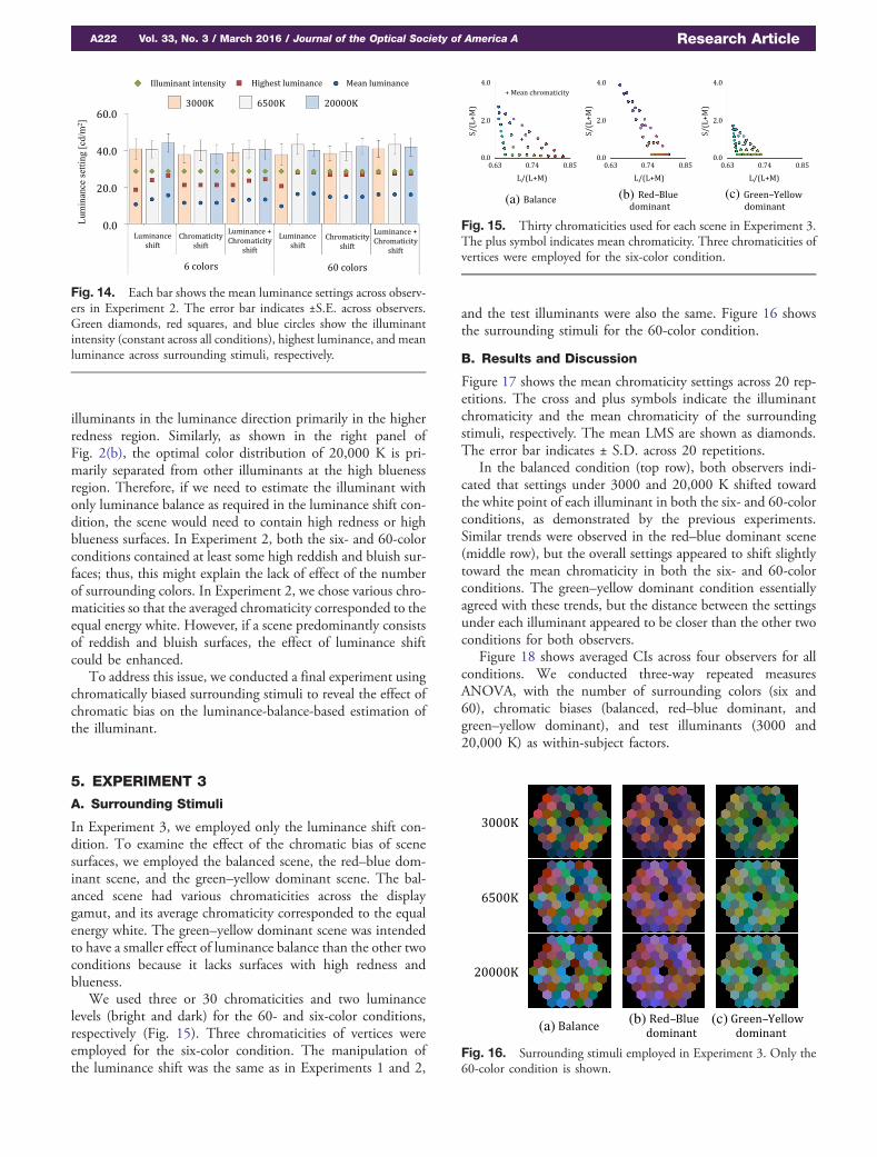
Figure 14 shows luminance settings for all conditions inExperiment 2. We conducted three-way repeated measuresANOVA, with the number of surrounding colors (six and 60),shift conditions (luminance shift, chromaticity shift, and lumi-nance and chromaticity shift), and test illuminants (3000,6500, and 20,000 K) as within-subject factors.

The results show that neither the main effects nor the inter-actionswere significant, suggesting that the estimated illuminantintensities were relatively stable regardless of the condition.

The main finding in Experiment 2 is that increasing thenumber of surrounding colors helps the estimation of the illu-minant in the chromaticity shift condition and the luminanceand chromaticity shift condition, while that in the luminanceshift condition was not affected. This suggests that these aremediated by different mechanisms.

As shown in the left panel of Fig. 2(b), the optimal colordistribution of 3000 K is separated from the other two

(a) (b) (c)

Fig. 12. Surrounding stimuli employed in Experiment 2. Only the60-color condition is shown.

Fig. 13. Averaged constancy indices across four observers inExperiment 2. Higher values indicate better color constancy. The errorbar indicates ±S.E. across four observers. The blue dashed lines are theconstancy index from Experiment 1 for comparison (2D and 3Dconditions were averaged).


illuminants in the luminance direction primarily in the higherredness region. Similarly, as shown in the right panel ofFig. 2(b), the optimal color distribution of 20,000 K is pri-marily separated from other illuminants at the high bluenessregion. Therefore, if we need to estimate the illuminant withonly luminance balance as required in the luminance shift con-dition, the scene would need to contain high redness or highblueness surfaces. In Experiment 2, both the six- and 60-colorconditions contained at least some high reddish and bluish sur-faces; thus, this might explain the lack of effect of the numberof surrounding colors. In Experiment 2, we chose various chro-maticities so that the averaged chromaticity corresponded to theequal energy white. However, if a scene predominantly consistsof reddish and bluish surfaces, the effect of luminance shiftcould be enhanced.

To address this issue, we conducted a final experiment usingchromatically biased surrounding stimuli to reveal the effect ofchromatic bias on the luminance-balance-based estimation ofthe illuminant.

5. EXPERIMENT 3


In Experiment 3, we employed only the luminance shift con-dition. To examine the effect of the chromatic bias of scenesurfaces, we employed the balanced scene, the red–blue dom-inant scene, and the green–yellow dominant scene. The bal-anced scene had various chromaticities across the displaygamut, and its average chromaticity corresponded to the equalenergy white. The green–yellow dominant scene was intendedto have a smaller effect of luminance balance than the other twoconditions because it lacks surfaces with high redness andblueness.

We used three or 30 chromaticities and two luminancelevels (bright and dark) for the 60- and six-color conditions,respectively (Fig. 15). Three chromaticities of vertices wereemployed for the six-color condition. The manipulation ofthe luminance shift was the same as in Experiments 1 and 2,

and the test illuminants were also the same. Figure 16 showsthe surrounding stimuli for the 60-color condition.


Figure 17 shows the mean chromaticity settings across 20 rep-etitions. The cross and plus symbols indicate the illuminantchromaticity and the mean chromaticity of the surroundingstimuli, respectively. The mean LMS are shown as diamonds.The error bar indicates ± S.D. across 20 repetitions.

In the balanced condition (top row), both observers indi-cated that settings under 3000 and 20,000 K shifted towardthe white point of each illuminant in both the six- and 60-colorconditions, as demonstrated by the previous experiments.Similar trends were observed in the red–blue dominant scene(middle row), but the overall settings appeared to shift slightlytoward the mean chromaticity in both the six- and 60-colorconditions. The green–yellow dominant condition essentiallyagreed with these trends, but the distance between the settingsunder each illuminant appeared to be closer than the other twoconditions for both observers.

Figure 18 shows averaged CIs across four observers for allconditions. We conducted three-way repeated measuresANOVA, with the number of surrounding colors (six and60), chromatic biases (balanced, red–blue dominant, andgreen–yellow dominant), and test illuminants (3000 and20,000 K) as within-subject factors.

Fig. 14. Each bar shows the mean luminance settings across observ-ers in Experiment 2. The error bar indicates ±S.E. across observers.Green diamonds, red squares, and blue circles show the illuminantintensity (constant across all conditions), highest luminance, and meanluminance across surrounding stimuli, respectively.

(a) (b) (c)

Fig. 15. Thirty chromaticities used for each scene in Experiment 3.The plus symbol indicates mean chromaticity. Three chromaticities ofvertices were employed for the six-color condition.

(a) (b) (c)

Fig. 16. Surrounding stimuli employed in Experiment 3. Only the60-color condition is shown.


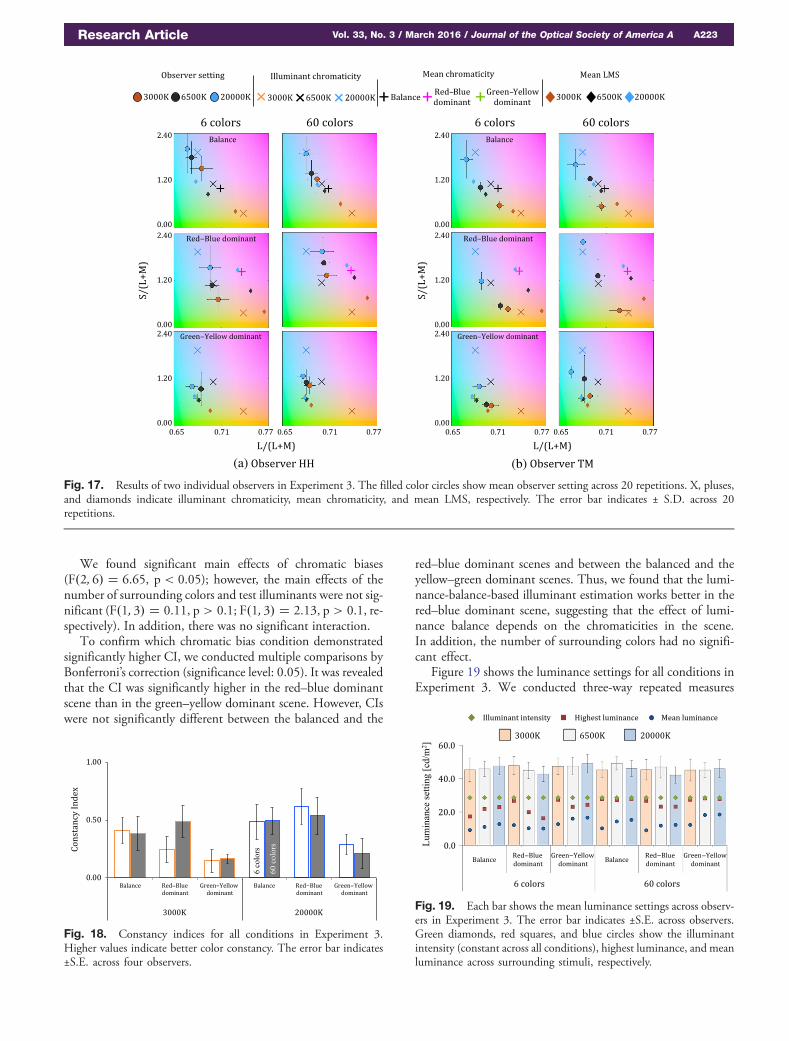
We found significant main effects of chromatic biases(F�2; 6� � 6.65, p < 0.05); however, the main effects of thenumber of surrounding colors and test illuminants were not sig-nificant (F�1; 3� � 0.11, p > 0.1; F�1; 3� � 2.13, p > 0.1, re-spectively). In addition, there was no significant interaction.

To confirm which chromatic bias condition demonstratedsignificantly higher CI, we conducted multiple comparisons byBonferroni’s correction (significance level: 0.05). It was revealedthat the CI was significantly higher in the red–blue dominantscene than in the green–yellow dominant scene. However, CIswere not significantly different between the balanced and the

red–blue dominant scenes and between the balanced and theyellow–green dominant scenes. Thus, we found that the lumi-nance-balance-based illuminant estimation works better in thered–blue dominant scene, suggesting that the effect of lumi-nance balance depends on the chromaticities in the scene.In addition, the number of surrounding colors had no signifi-cant effect.

Figure 19 shows the luminance settings for all conditions inExperiment 3. We conducted three-way repeated measures

(a) (b)

Fig. 17. Results of two individual observers in Experiment 3. The filled color circles show mean observer setting across 20 repetitions. X, pluses,and diamonds indicate illuminant chromaticity, mean chromaticity, and mean LMS, respectively. The error bar indicates ± S.D. across 20repetitions.

Fig. 18. Constancy indices for all conditions in Experiment 3.Higher values indicate better color constancy. The error bar indicates±S.E. across four observers.

Fig. 19. Each bar shows the mean luminance settings across observ-ers in Experiment 3. The error bar indicates ±S.E. across observers.Green diamonds, red squares, and blue circles show the illuminantintensity (constant across all conditions), highest luminance, and meanluminance across surrounding stimuli, respectively.


ANOVA, with the number of surrounding colors (six and 60),chromatic biases (balanced, red–blue dominant, and yellow–green dominant), and test illuminants (3000 and 20,000 K)as within-subject factors.

No main effect was found to be significant. However, theinteraction between the chromatic bias and the test illuminantwas significant (F�4; 12� � 3.74, p < 0.05). Further analysisof the simple main effect revealed that the luminance settingsamong chromatic balance conditions were significantly differ-ent for the 20,000 K condition but not for the 3000 K con-dition. Multiple comparisons using Bonferroni’s correction(significance level: 0.05) revealed that, in the 20,000 K condi-tion, the luminance setting was significantly higher in the green–yellow dominant scene than in the red–blue dominant scene.

6. MODEL COMPARISON

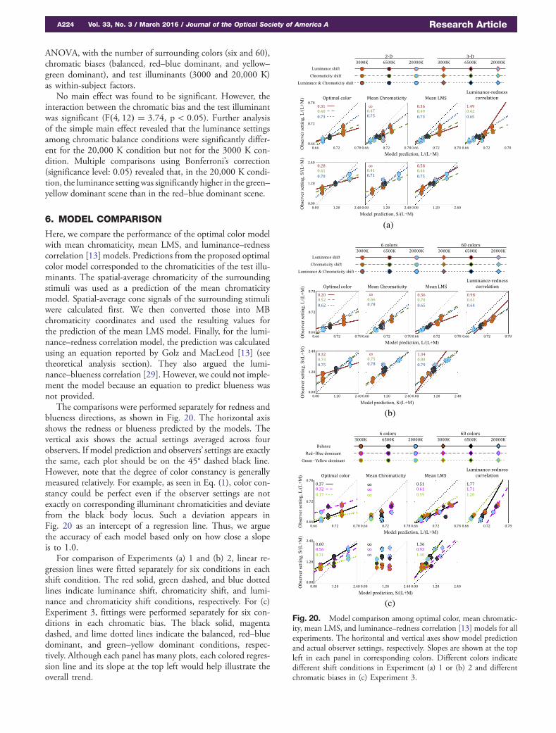
Here, we compare the performance of the optimal color modelwith mean chromaticity, mean LMS, and luminance–rednesscorrelation [13] models. Predictions from the proposed optimalcolor model corresponded to the chromaticities of the test illu-minants. The spatial-average chromaticity of the surroundingstimuli was used as a prediction of the mean chromaticitymodel. Spatial-average cone signals of the surrounding stimuliwere calculated first. We then converted those into MBchromaticity coordinates and used the resulting values forthe prediction of the mean LMS model. Finally, for the lumi-nance–redness correlation model, the prediction was calculatedusing an equation reported by Golz and MacLeod [13] (seetheoretical analysis section). They also argued the lumi-nance–blueness correlation [29]. However, we could not imple-ment the model because an equation to predict blueness wasnot provided.

The comparisons were performed separately for redness andblueness directions, as shown in Fig. 20. The horizontal axisshows the redness or blueness predicted by the models. Thevertical axis shows the actual settings averaged across fourobservers. If model prediction and observers’ settings are exactlythe same, each plot should be on the 45° dashed black line.However, note that the degree of color constancy is generallymeasured relatively. For example, as seen in Eq. (1), color con-stancy could be perfect even if the observer settings are notexactly on corresponding illuminant chromaticities and deviatefrom the black body locus. Such a deviation appears inFig. 20 as an intercept of a regression line. Thus, we arguethe accuracy of each model based only on how close a slopeis to 1.0.

For comparison of Experiments (a) 1 and (b) 2, linear re-gression lines were fitted separately for six conditions in eachshift condition. The red solid, green dashed, and blue dottedlines indicate luminance shift, chromaticity shift, and lumi-nance and chromaticity shift conditions, respectively. For (c)Experiment 3, fittings were performed separately for six con-ditions in each chromatic bias. The black solid, magentadashed, and lime dotted lines indicate the balanced, red–bluedominant, and green–yellow dominant conditions, respec-tively. Although each panel has many plots, each colored regres-sion line and its slope at the top left would help illustrate theoverall trend.

(a)

(b)

(c)

Fig. 20. Model comparison among optimal color, mean chromatic-ity, mean LMS, and luminance–redness correlation [13] models for allexperiments. The horizontal and vertical axes show model predictionand actual observer settings, respectively. Slopes are shown at the topleft in each panel in corresponding colors. Different colors indicatedifferent shift conditions in Experiment (a) 1 or (b) 2 and differentchromatic biases in (c) Experiment 3.


In (a) Experiment 1, for the chromaticity shift conditionand luminance and chromaticity shift condition, performanceis roughly similar for all models for both redness and bluenesspredictions. Therefore, once the chromaticity change is avail-able to estimate an illuminant, each model can sufficiently pre-dict the observer settings. However, for the luminance shiftcondition, the mean chromaticity model does not work becausethe chromaticities of all surfaces were constant across the testilluminants and, thus, incorrectly provided the same estimationfor all test illuminants. In contrast, our optimal color model canperform prediction to some extent, and the mean LMS andluminance–redness correlation models worked sufficiently. Asimilar trend was observed in Experiment 2.

In (c) Experiment 3, we employed only the luminance shiftcondition; therefore, the mean chromaticity did not account forany of the results. Again, our model predicts the results to someextent. However, the mean LMS model also worked well, andthe redness–luminance correlation model worked reliably, espe-cially for the green–yellow dominant condition.

Overall, for most conditions, the mean LMS and lumi-nance–redness correlation models showed good predictions.However, in our previous study [21], we tested a conditionwhere the mean LMS values were equated across the test illu-minants (Experiment 4). It turned out that, under such a con-dition, the observer’s settings were shifted to the oppositedirection from the illuminant chromaticity. Therefore, evenif the mean LMS is a good predictor in the present study, itseems difficult to establish a basis for further discussion.

7. GENERAL DISCUSSION

Despite substantial psychophysical color constancy research,only a few studies have investigated the luminance contributionto color constancy. The present study was aimed at reinforcinga previous finding, i.e., luminance balance contributes to theestimation of an illuminant [21]. The luminance shift condi-tion simulated the extreme situation in which the chromatic-ities of all surfaces in a scene happen to be exactly the sameacross the illuminants; thus, the visual system had to assessthe illuminant based only on luminance balance. Althoughsuch a difficult situation never occurs in the real world, surpris-ingly, the visual system can resolve the ambiguity of chroma-ticity and estimate the illuminant to some extent. Needless tosay, chromaticity-based models do not account for this ability ofthe visual system. These findings strongly confirm that the lu-minance balance of surfaces plays an important role in achiev-ing color constancy.

In Experiment 1, we tested whether stimulus dimensionalitycould affect illuminant estimation. However, the results did notshow any effect. There has been an implicit expectation thatcolor constancy should improve for 3D stimuli because thoseappear more informative compared to 2D stimuli. While somestudies have supported this idea, other studies did not show thiseffect. Therefore, whether 3D stimuli can improve color con-stancy remains controversial. However, in the present study, weused a shade to make hexagons appear as cubes, whereas otherstudies used various manipulations to create a 3D environment[9,21–26]. Therefore, the present results may have been due tothe different stimuli manipulation method. It is possible that

the stimulus shape does not matter for the optimal color hy-pothesis; however, concrete conclusions require the testing ofother shapes.

In Experiment 2, it was shown that chromatic variation en-hances the effect of chromaticity shift. In contrast, chromaticvariation does not appear to affect the luminance-balance effect.In terms of the optimal color hypothesis, low saturated colorsare less helpful because they could be within more than oneilluminant gamut. The six-color condition employed threechromaticities chosen from the vertices of the chromaticity tri-angle (Fig. 11) and thus contained the highest redness andblueness surfaces. This might be the reason why we couldnot obtain improvement by increasing the number of sur-rounding colors. The important implication from this resultis that the visual system places greater weight on highly satu-rated colors as well as bright colors [8] when estimating an il-luminant.

In Experiment 3, we investigated the luminance-balance ef-fect in chromatically biased scenes. The results showed thatobservers made better estimations of illuminants for thered–blue dominant scene compared to the green–yellow dom-inant scene, suggesting that the accuracy of illuminant estima-tion based on luminance balance depends on the chromaticityin the scene. Although we specified a condition in which theluminance balance could work better, the degree of color con-stancy was still approximately 47% on average for the red–bluedominant condition, which is still generally less than the CI inthe chromatic shift conditions. This result implies that the roleof luminance in estimating an illuminant is limited to specifythe direction of the illuminant color so that the visual systemcan maintain color constancy when a scene has chromatic am-biguity.

The observer’s task employed in the present study allowed usto see the estimated illuminant chromaticity and intensity si-multaneously. While the accuracy of the estimated chromaticitywas dependent on the conditions, the observer demonstratedsomewhat stable estimation of the illuminant intensity.However, the estimated intensity was substantially and consis-tently higher than the actual intensity of the test illuminant.This implies that, even though we employed optimal colorsfor surrounding stimuli, the visual system interpreted themas darker surfaces. This in turn suggests that the assumptionof surfaces internalized in the visual system is less restricted thanoptimal colors. Note that the illuminant gamut extends in theluminance direction when its intensity increases. Therefore, interms of the optimal color hypothesis, accurate estimation ofilluminant intensity is required for a good estimation of illu-minant chromaticity. For example, even if a scene contains abright reddish surface, a bluish illuminant gamut could holdall surfaces in the scene when the visual system estimatesthe illuminant intensity at a high level. This might have causedthe imperfect constancy observed in the present study. In thefuture, a broader investigation is required to assess the overallrelationship between the estimations of intensity and colortemperature.

There has been a long-standing argument about the methodof measuring color constancy. Various methods have beenproposed, such as asymmetric matching [23], achromatic


adjustment [30], color naming [31], and classification betweenmaterial change and illuminant change [32]. The present studyemployed achromatic adjustment based on the paper-matchcriterion rather than appearance match. It has often been re-ported that this operational color constancy shows a relativelyhigh degree [23]. Nevertheless, CIs observed in luminance shiftconditions were small. Thus, it would be difficult to extract thecontribution of luminance in illuminant estimation using anappearance-based task.

Themethod of quantifying the degree of color constancy alsoremains controversial. In the present study, we employed a CI asEq. (1), but this simple measure fails to reflect the data trend ifshifts are in the opposite direction from the expected point. Wefound that one observer showed such opposite shifts under sev-eral conditions. However, the indices were nearly zero in thosecases; thus, they did not affect the overall trends significantly.

Note that no model consistently provided satisfactory esti-mation for all conditions tested in the present study. This im-plies that the visual system does not rely on a specific algorithmto achieve color constancy. Although all models exploited theglobal statistics across the entire scene, many studies haveagreed that multiple mechanisms underlie human color con-stancy, such as an adaptation, simultaneous contrast, and evenfamiliarity or memory. Thus, the visual system could exploit themost reliable cue in a given situation, which might cause diffi-culty in specifying a consistently reliable model.

The neural mechanism for color constancy remains largelyunclear. While there appears to be an important role in theretina, such as adaptation [33], color constancy could workwithout taking adaptation time [34]. Higher cortical mecha-nisms, such as V4, have also been identified [35–37]. Our pro-posed model essentially assumes the opponent level process,such as the mean chromaticity model. In our model compari-son, we found that the mean LMS provided relatively reliableestimation for the most of the tested condition. The mean LMSmodel implies that illuminant estimation can be completed bysimply taking the average of each class of cone signals beforeentering the opponent level process. However, it is possible thatthese are the average luminance-weighted chromaticities ratherthan actual cone signals.

The key idea of the proposed model stems from the expect-ation that the visual system internalizes possible references(optimal color distributions). In this notion, the given sceneinformation is used to determine which internalized referencewe should select to discount the influence of the illuminantproperly. Thus, our model appears to oppose to frameworksthat rely completely on external sources in a scene to set a refer-ence, such as anchoring theory [38]. It is possible that the visualsystem uses both; however, in any case, we require a furtherinvestigation to reveal whether the visual system can utilizeprior knowledge about the world.

One might suspect that it is more reasonable to assume thatthe visual system internalizes the shape of the natural scene dis-tribution rather than the optimal color distribution because op-timal colors do not exist in the real world. Although the presentstudy cannot rule out this possibility, one way to assess the fea-sibility of the proposed method would be to identify how colorsare distributed in the world. As shown in Fig. 2(b), the shape of

optimal colors and natural object distribution are somewhatsimilar, implying that the visual system has access to the relativeshape of the optimal color distribution. However, these naturalobjects were a limited number of samples, and it appears diffi-cult to determine the actual surface gamut in the natural world.Pointer [39] has argued how large the gamut of real surfaces(known as Pointer’s limit) would be, but this is also inconclu-sive. Another clue could be the mysterious relationship betweenthe luminous threshold and the luminance of optimal color[20]. Since there is nothing connecting natural objects withthe luminosity threshold, this seems to support what the visualsystem knows to be the theoretical limit of surface colors ratherthan the natural scene distribution.

Funding. Japan Society for the Promotion of Science(JSPS) KAKENHI (23730696, 26780413).

Acknowledgment. This work was supported in part byJapan Society for the Promotion of Science (JSPS) KAKENHIgrants 23730696 and 26780413 to K.F.

REFERENCES

1. D. H. Foster, “Color constancy,” Vis. Res. 51, 674–700 (2011).2. H. E. Smithson, “Sensory, computational and cognitive components of

human colour constancy,” Philos. Trans. R. Soc. B 360, 1329–1346(2005).

3. A. Werner, “Spatial and temporal aspects of chromatic adaptation andtheir functional significance for colour constancy,” Vis. Res. 104,80–89 (2014).

4. J. von Kries, “Influence of adaptation on the effects produced byluminous stimuli,” in Sources of Color Science, D. L. MacAdam, ed.(MIT, 1905), pp. 120–126.

5. H. E. Ives, “The relation between the color of the illuminant and thecolor of the illuminated object,” Trans. Illuminant. Eng. Soc. 7,62–72 (1912).

6. M. Olkkonen, T. Hansen, and K. R. Gegenfurtner, “Color appearanceof familiar objects: effects of object shape, texture, and illuminationchanges,” J. Vis. 8(5), 13 (2008).

7. D.H.FosterandS.M.C.Nascimento, “Relationalcolourconstancy frominvariant cone-excitation ratios,” Proc. Biol. Sci. 257, 115–121 (1994).

8. S. Tominaga, S. Ebisui, and B. A. Wandell, “Scene illuminant classi-fication: brighter is better,” J. Opt. Soc. Am. A 18, 55–64 (2001).

9. J. N. Yang and S. K. Shevell, “Stereo disparity improves color con-stancy,” Vis. Res. 42, 1979–1989 (2002).

10. K. Fukuda and K. Uchikawa, “Color constancy in a scene with brightcolors that do not have a fully natural surface appearance,” J. Opt.Soc. Am. A 31, A239–A246 (2014).

11. G. Buchsbaum, “A spatial processor model for object color percep-tion,” J. Franklin Institute 310, 1–26 (1980).

12. R. O. Brown, “The world is not gray,” Invest. Ophthalmol. Vis. Sci. 35,2165 (1994).

13. J. Golz and D. I. A. MacLeod, “Influence of scene statistics on colourconstancy,” Nature 415, 637–640 (2002).

14. D. Macadam, “The theory of the maximum visual efficiency of coloredmaterials,” J. Opt. Soc. Am. A 25, 249–252 (1935).

15. D. Macadam, “Maximum visual efficiency of colored materials,” J. Opt.Soc. Am. A 25, 361–367 (1935).

16. A. Stockman and L. T. Sharpe, “Spectral sensitivities of the middle-and long-wavelength sensitive cones derived from measurements inobservers of known genotype,” Vis. Res. 40, 1711–1737 (2000).

17. D. I. A. MacLeod and R. M. Boynton, “Chromaticity diagram showingcone excitation by stimuli of equal luminance,” J. Opt. Soc. Am. A 69,1183–1186 (1979).

18. D. A. Forsyth, “A novel algorithm for color constancy,” Int. J. Comput.Vis. 5, 5–35 (1990).


19. R. Brown, “Background and illuminants: the yin and yang of colourconstancy,” in Colour Perception: Mind and the Physical World, R.Mausfeld and D. Heyer, eds. (Oxford University, 2003), pp. 247–272.

20. K. Uchikawa, K. Koida, T. Meguro, Y. Yamauchi, and I. Kuriki,“Brightness, not luminance, determines transition from thesurface-color to the aperture-color mode for colored lights,” J. Opt.Soc. Am. A 18, 737–746 (2001).

21. K. Uchikawa, K. Fukuda, Y. Kitazawa, and D. I. A. MacLeod,“Estimating illuminant color based on luminance balance of surfaces,”J. Opt. Soc. Am. A 29, A133–A143 (2012).

22. M. Hedrich, M. Bloj, and A. I. Ruppetsberg, “Color constancy improvesfor real 3D objects,” J. Vis. 9(4), 16 (2009).

23. L. Arend and A. Reeves, “Simultaneous color constancy,” J. Opt. Soc.Am. A 3, 1743–1751 (1986).

24. B. Xiao, B. Hurst, L. Maclntyre, and D. H. Brainard, “The color con-stancy of three-dimensional objects,” J. Vis. 12(4), 6 (2012).

25. A. Werner, “The influence of depth segmentation on colour con-stancy,” Perception 35, 1171–1184 (2006).

26. Y. Mizokami and H. Yaguchi, “Color constancy influenced byunnatural spatial structure,” J. Opt. Soc. Am. A 31, A179–A185(2014).

27. V. M. N. de Almeida, P. T. Fiadeiro, and S. M. C. Nascimento, “Effectof scene dimensionality on colour constancy with real three-dimen-sional scenes and objects,” Perception 39, 770–779 (2010).

28. J. M. Kraft, S. I. Maloney, and D. H. Brainard, “Surface-illuminantambiguity and color constancy: effects of scene complexity and depthcues,” Perception 31, 247–263 (2002).

29. D. I. A. MacLeod and J. Golz, “A computational analysis of colour con-stancy,” in Colour Perception: Mind and the Physical World, R.Mausfeld and D. Heyer, eds. (Oxford University, 2003), pp. 205–246.

30. D. H. Brainard, “Color constancy in the nearly natural image. 2.Achromatic loci,” J. Opt. Soc. Am. A 15, 307–325 (1998).

31. J. M. Troost and C. M. M. de Weert, “Naming versus matching in colorconstancy,” Percept. Psychophys. 50, 591–602 (1991).

32. B. J. Craven and D. H. Foster, “An operational approach to colour con-stancy,” Vis. Res. 32, 1359–1366 (1992).

33. H. E. Smithson and Q. Zaidi, “Colour constancy in context: roles forlocal adaptation and levels of reference,” J. Vis. 4(9), 3 (2004).

34. O. Rinner and K. R. Gegenfurtner, “Cone contributions to colour con-stancy,” Perception 31, 733–746 (2002).

35. M. Kusunoki, K. Moutoussis, and S. Zeki, “Effect of backgroundcolors on the tuning of color-selective cells in monkey area V4,”J. Neurophys. 95, 3047–3059 (2006).

36. V. Walsh, D. Carden, S. R. Butler, and J. J. Kulikowski, “The effects ofV4 lesions on the visual abilities of macaques: hue discrimination andcolour constancy,” Behav. Brain. Res. 53, 51–62 (1993).

37. H. M. Wild, S. R. Butler, D. Carden, and J. J. Kulikowski, “Primatecortical area V4 important for colour constancy but not wavelengthdiscrimination,” Nature 313, 133–135 (1985).

38. A. Gilchrist, C. Kossyfidis, F. Bonato, T. Agostini, J. Cataliotti, X. Li,B. Spehar, V. Annan, and E. Economou, “An anchoring theory oflightness perception,” Psychol. Rev. 106, 795–834 (1999).

39. M. R. Pointer, “The gamut of real surface colours,” Col. Res. Appl. 5,145–155 (1980).


Effects of surrounding stimulus properties on color...

Documents

Transcript of Effects of surrounding stimulus properties on color...