Economics of Behavioral Finance Lecture 3

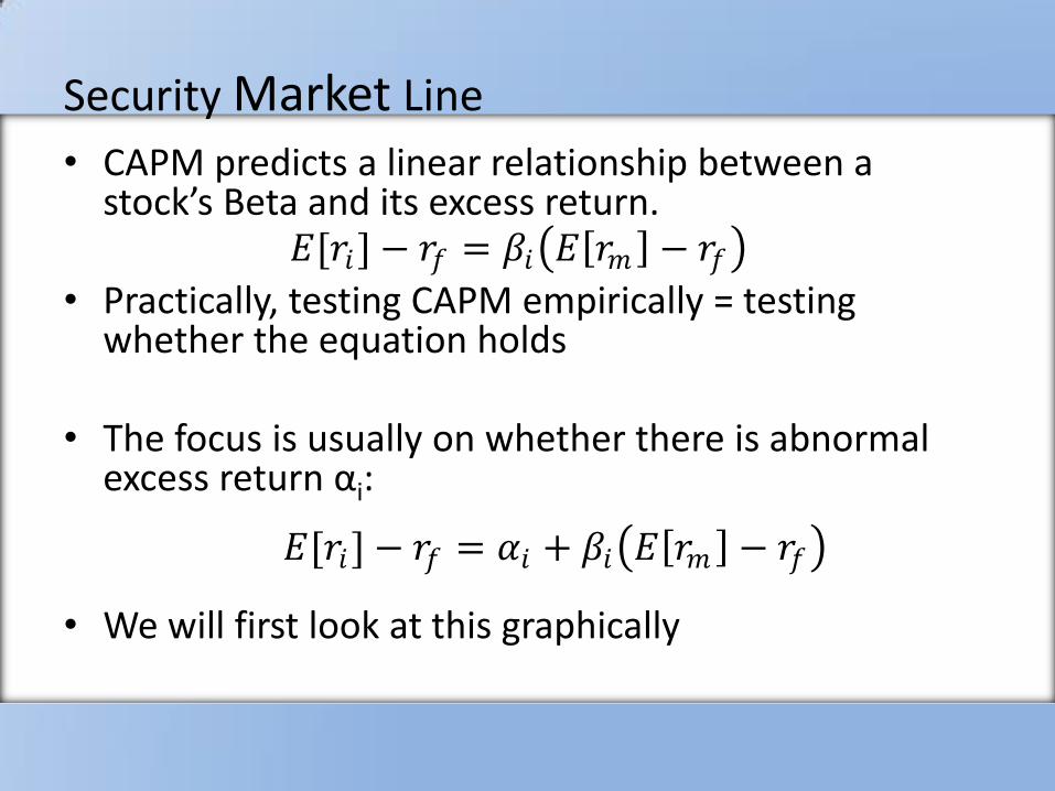
Security Market Line

• CAPM predicts a linear relationship between a stock’s Beta and its excess return.

• Practically, testing CAPM empirically = testing

whether the equation holds

• The focus is usually on whether there is abnormal excess return αi:

• We will first look at this graphically

𝐸[𝑟𝑖]− 𝑟𝑓 = 𝛽𝑖 𝐸 𝑟𝑚 − 𝑟𝑓

𝐸[𝑟𝑖]− 𝑟𝑓 = 𝛼𝑖 + 𝛽𝑖 𝐸 𝑟𝑚 − 𝑟𝑓

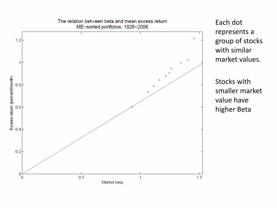
Each dot represents a group of stocks with similar market values.

Stocks with smaller market value have higher Beta

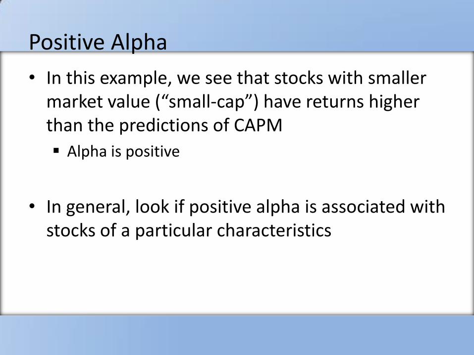
Positive Alpha

• In this example, we see that stocks with smaller market value (“small-cap”) have returns higher than the predictions of CAPM

Alpha is positive

• In general, look if positive alpha is associated with stocks of a particular characteristics

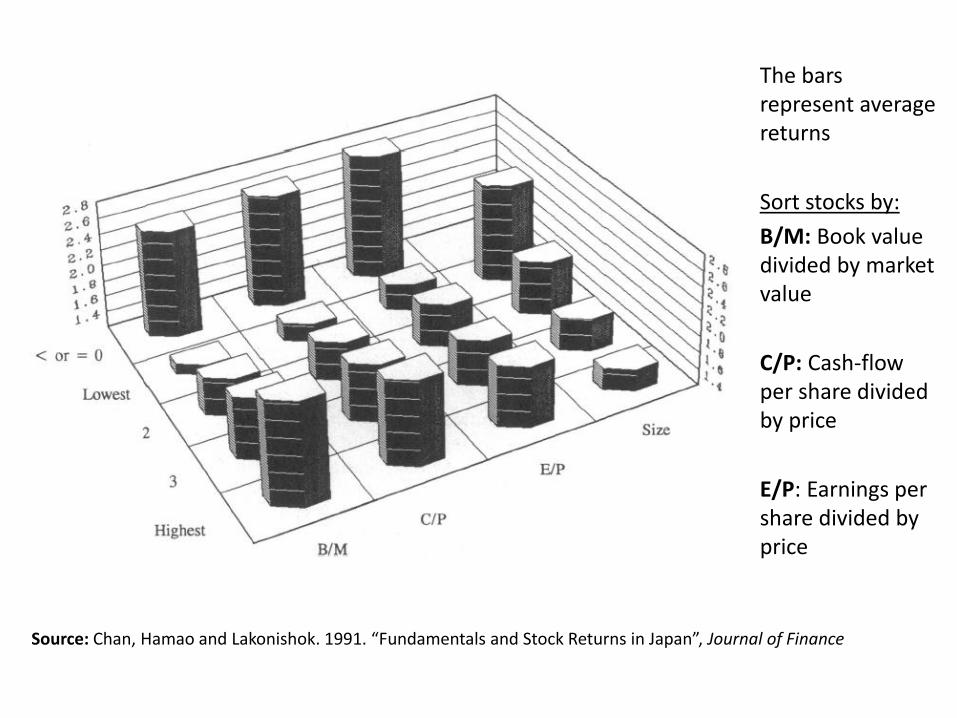
The bars represent average returns

Sort stocks by:

B/M: Book value divided by market value

C/P: Cash-flow per share divided by price

E/P: Earnings per share divided by price

Source: Chan, Hamao and Lakonishok. 1991. “Fundamentals and Stock Returns in Japan”, Journal of Finance

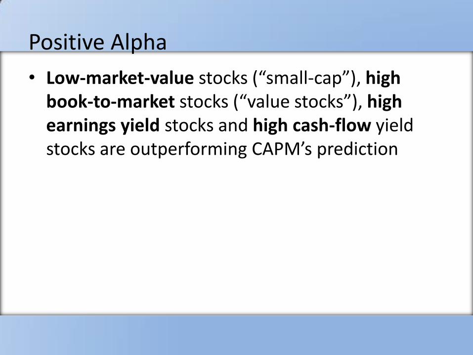
Positive Alpha

• Low-market-value stocks (“small-cap”), high book-to-market stocks (“value stocks”), high earnings yield stocks and high cash-flow yield stocks are outperforming CAPM’s prediction

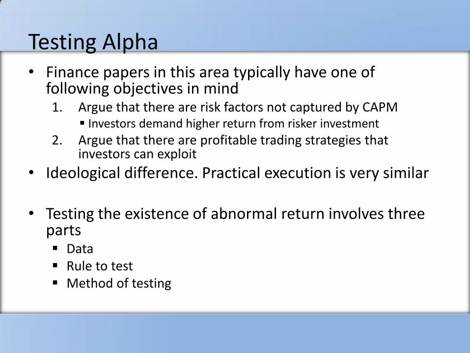
Testing Alpha • Finance papers in this area typically have one of

following objectives in mind 1. Argue that there are risk factors not captured by CAPM

Investors demand higher return from risker investment

2. Argue that there are profitable trading strategies that investors can exploit

• Ideological difference. Practical execution is very similar

• Testing the existence of abnormal return involves three parts Data Rule to test Method of testing

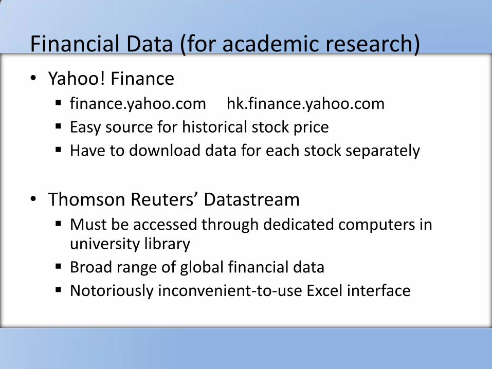
Financial Data (for academic research)

• Yahoo! Finance finance.yahoo.com hk.finance.yahoo.com

Easy source for historical stock price

Have to download data for each stock separately

• Thomson Reuters’ Datastream Must be accessed through dedicated computers in

university library

Broad range of global financial data

Notoriously inconvenient-to-use Excel interface

Financial Data (for academic research)

• Wharton Research Data Service (WRDS)

wrds.wharton.upenn.edu

Centralized online source for multiple datasets

Institutional subscription

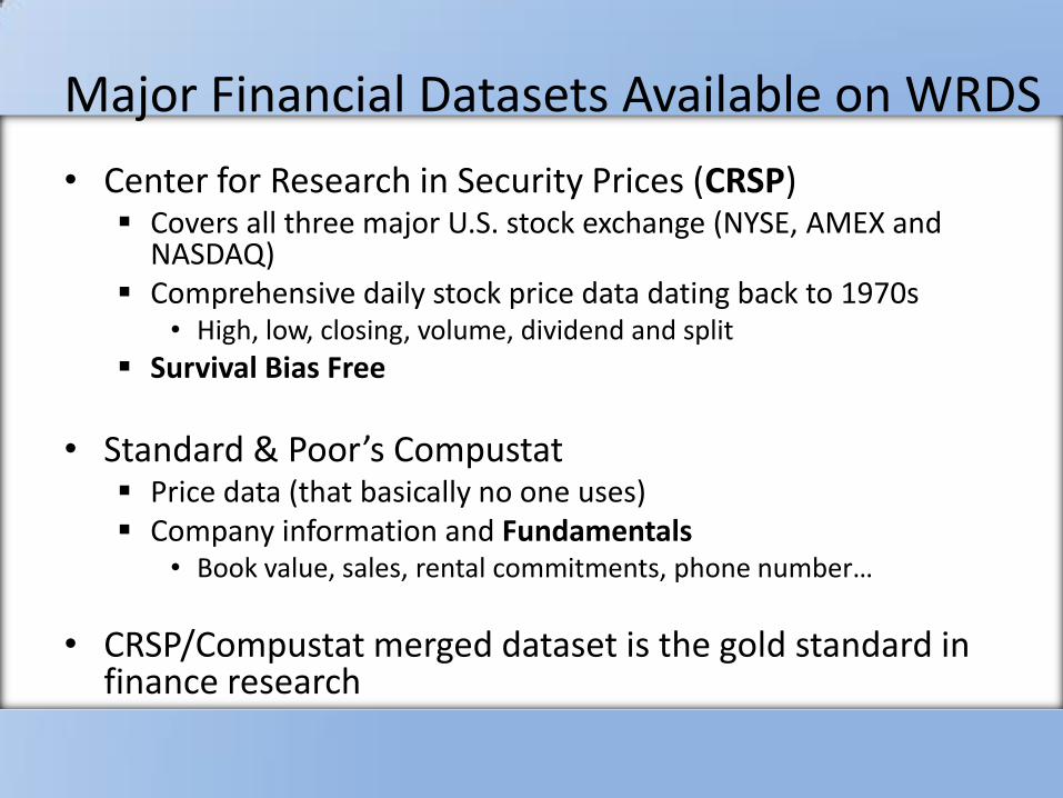
Major Financial Datasets Available on WRDS

• Center for Research in Security Prices (CRSP) Covers all three major U.S. stock exchange (NYSE, AMEX and

NASDAQ) Comprehensive daily stock price data dating back to 1970s

• High, low, closing, volume, dividend and split

Survival Bias Free

• Standard & Poor’s Compustat Price data (that basically no one uses) Company information and Fundamentals

• Book value, sales, rental commitments, phone number…

• CRSP/Compustat merged dataset is the gold standard in finance research

Major Financial Datasets Available on WRDS

• Thomson Reuters’ I/B/E/S

Analyst forecast of company earnings

• Our class account for WRDS

Username: econ4470

Password: CUHK_elb_403

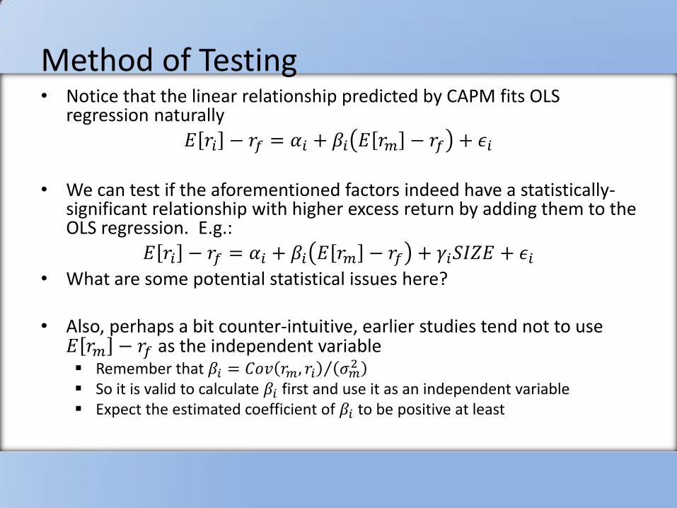
Method of Testing • Notice that the linear relationship predicted by CAPM fits OLS

regression naturally

𝐸 𝑟𝑖 − 𝑟𝑓 = 𝛼𝑖 + 𝛽𝑖 𝐸 𝑟𝑚 − 𝑟𝑓 + 𝜖𝑖

• We can test if the aforementioned factors indeed have a statistically-

significant relationship with higher excess return by adding them to the OLS regression. E.g.:

𝐸 𝑟𝑖 − 𝑟𝑓 = 𝛼𝑖 + 𝛽𝑖 𝐸 𝑟𝑚 − 𝑟𝑓 + 𝛾𝑖𝑆𝐼𝑍𝐸 + 𝜖𝑖

• What are some potential statistical issues here?

• Also, perhaps a bit counter-intuitive, earlier studies tend not to use 𝐸 𝑟𝑚 − 𝑟𝑓 as the independent variable Remember that 𝛽𝑖 = 𝐶𝑜𝑣 𝑟𝑚, 𝑟𝑖 𝜎𝑚

2 So it is valid to calculate 𝛽𝑖 first and use it as an independent variable Expect the estimated coefficient of 𝛽𝑖 to be positive at least

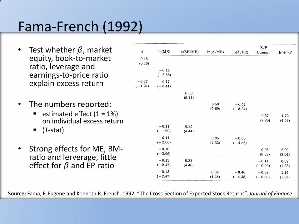
Fama-French (1992)

• Test whether 𝛽, market equity, book-to-market ratio, leverage and earnings-to-price ratio explain excess return

• The numbers reported: estimated effect (1 = 1%)

on individual excess return (T-stat)

• Strong effects for ME, BM-ratio and lerverage, little effect for 𝛽 and EP-ratio

Source: Fama, F. Eugene and Kenneth R. French. 1992. “The Cross-Section of Expected Stock Returns”, Journal of Finance

Fama-French (1993) • It is important to note that small-cap stocks and

value stocks are having abnormal excess return under CAPM, which is a very simple model

• A more sophisticated model perhaps?

• Idea: Value stocks and small-cap stocks are each exposed to common factors not shared by growth, large-cap stocks

• From data we can construct indexes that represent these factors

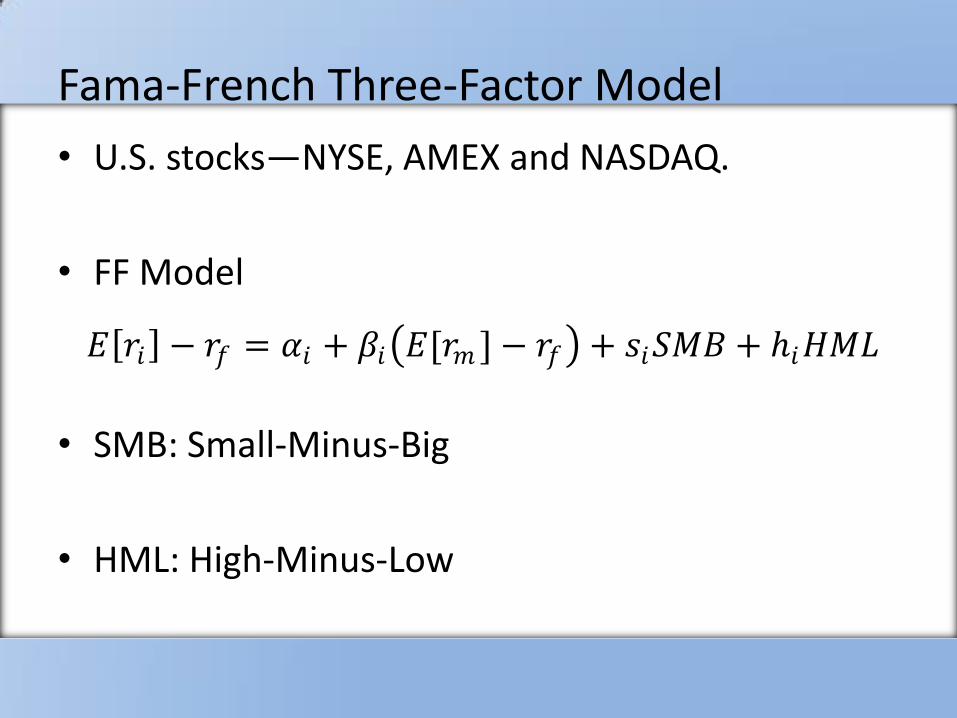
Fama-French Three-Factor Model

• U.S. stocks—NYSE, AMEX and NASDAQ.

• FF Model

• SMB: Small-Minus-Big

• HML: High-Minus-Low

𝐸 𝑟𝑖 − 𝑟𝑓 = 𝛼𝑖 + 𝛽𝑖 𝐸[𝑟𝑚 ]− 𝑟𝑓 + 𝑠𝑖𝑆𝑀𝐵 + ℎ𝑖𝐻𝑀𝐿

Fama-French Three-Factor Model

• Group stocks according to their market value and book-to-market value

• SMB is average of top three minus bottom three

• HML is average of right two minus left two

• Up-to-date SMB and HML data can be downloaded from Kenneth French’s website.

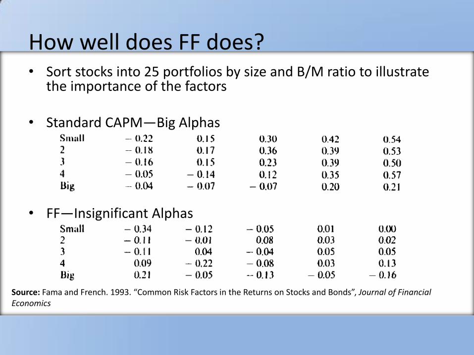
How well does FF does? • Sort stocks into 25 portfolios by size and B/M ratio to illustrate

the importance of the factors

• Standard CAPM—Big Alphas

• FF—Insignificant Alphas

Source: Fama and French. 1993. “Common Risk Factors in the Returns on Stocks and Bonds”, Journal of Financial Economics

So FF Works Great…

• But what do the SMB and HML factors actually represent?

Efficient-market believers: SMB and HML represent risks

Inefficient-market believers: represent mistakes made by investors

• Hard to quantify what risks the factors represent

Whatever risks they are, they should show up in form of lower return at some periods of time

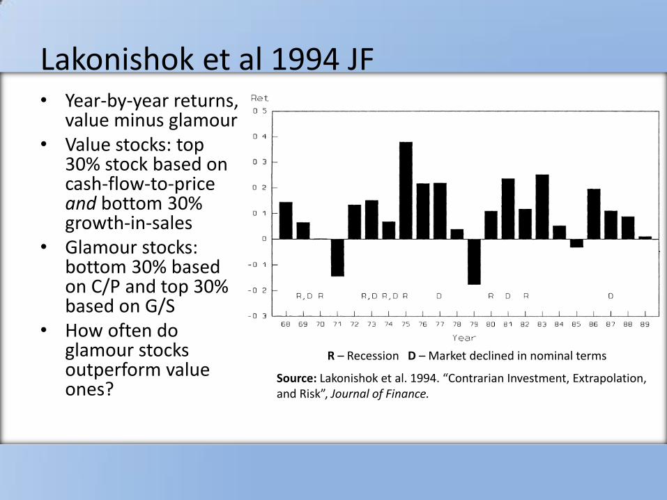
Lakonishok et al 1994 JF

Source: Lakonishok et al. 1994. “Contrarian Investment, Extrapolation, and Risk”, Journal of Finance.

• Year-by-year returns, value minus glamour

• Value stocks: top 30% stock based on cash-flow-to-price and bottom 30% growth-in-sales

• Glamour stocks: bottom 30% based on C/P and top 30% based on G/S

• How often do glamour stocks outperform value ones?

R – Recession D – Market declined in nominal terms

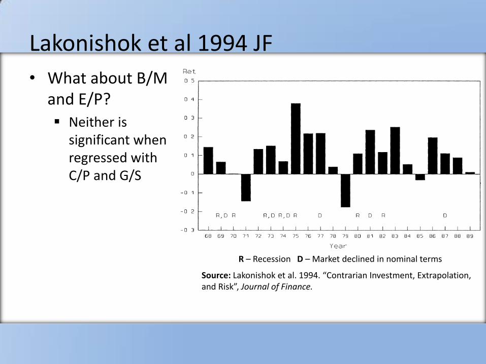
Lakonishok et al 1994 JF

Source: Lakonishok et al. 1994. “Contrarian Investment, Extrapolation, and Risk”, Journal of Finance.

• What about B/M and E/P?

Neither is significant when regressed with C/P and G/S

R – Recession D – Market declined in nominal terms

Daniel and Titman 1997 JF • If the factors represent risks, we should see higher return for assets that are

more correlated with the factors • This should be true even within each size-B/M-sorted portfolio • Sort stocks based on B/M, size and correlation with the HML factor • 1 = 1% average excess return

Source: Daniel and Titman. 1997. “Evidence on the Characteristics of Cross Sectional Variation in Stock Returns”, Journal of Finance.

Summary

• There is no evidence that FF factors represent systemic risks

• Baseline: Fama-French is an empirical model.

Stock Return Anomalies (relative to CAPM)

• Value Effect

Stocks with high book-to-market ratios (“value” stocks) have higher returns than low B/M (“growth”) stocks.

• Size Effect

Stocks with low market value (“small” stocks) have a higher return than large stocks.

Stock Return Anomalies (relative to CAPM)

• Momentum

Stocks that have done well over 3 months to 1 year (“momentum” stocks) have high subsequent returns.

• Reversal

Stocks that have done well the past 1-4 years earn low returns.

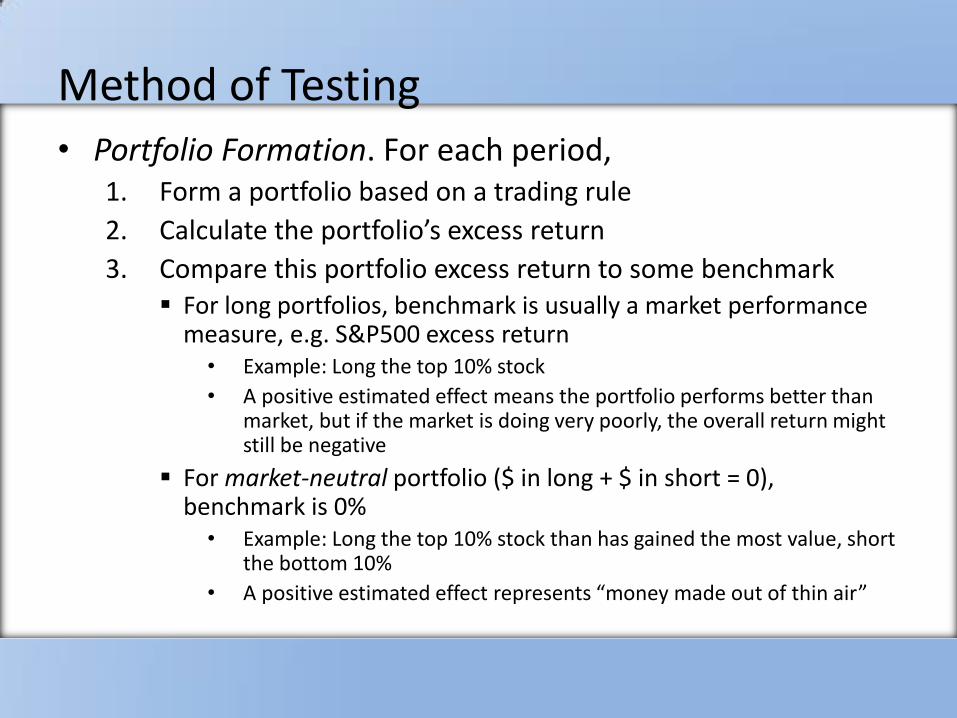
Method of Testing • Portfolio Formation. For each period,

1. Form a portfolio based on a trading rule

2. Calculate the portfolio’s excess return

3. Compare this portfolio excess return to some benchmark For long portfolios, benchmark is usually a market performance

measure, e.g. S&P500 excess return • Example: Long the top 10% stock

• A positive estimated effect means the portfolio performs better than market, but if the market is doing very poorly, the overall return might still be negative

For market-neutral portfolio ($ in long + $ in short = 0), benchmark is 0% • Example: Long the top 10% stock than has gained the most value, short

the bottom 10%

• A positive estimated effect represents “money made out of thin air”

Method of Testing

• Suppose we discovered a rule based on some stock data. Can we just compare the portfolio to the benchmark using the same data?

Momentum and Reversal

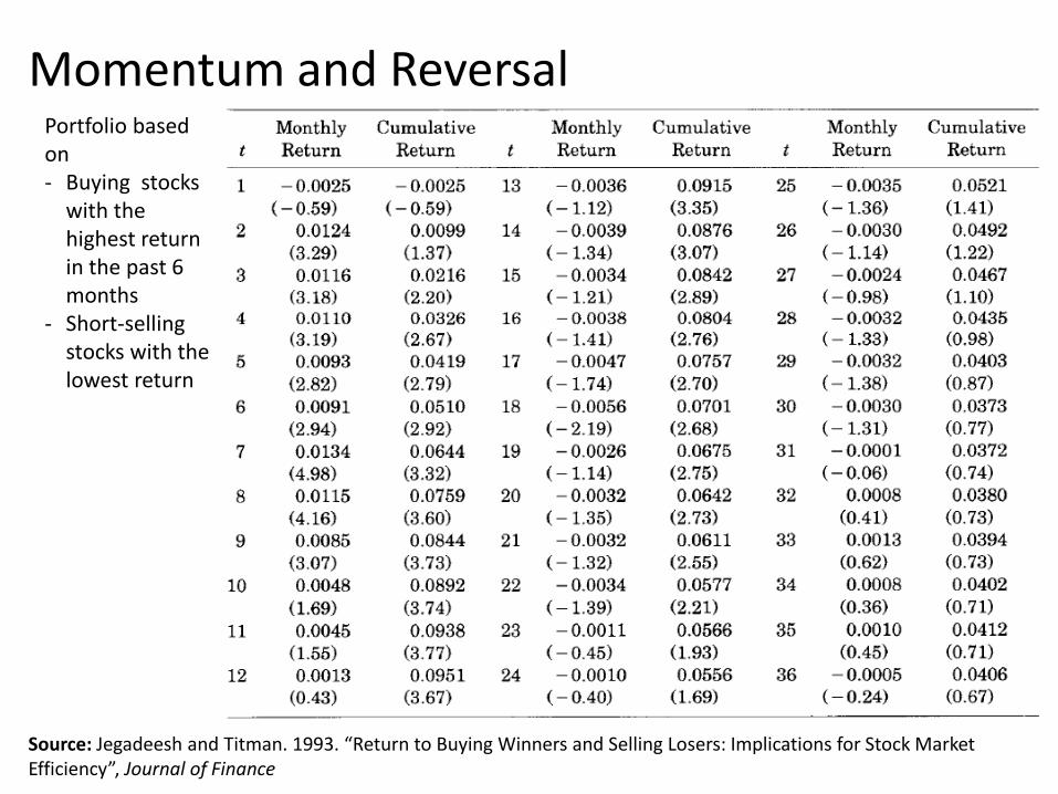
Source: Jegadeesh and Titman. 1993. “Return to Buying Winners and Selling Losers: Implications for Stock Market Efficiency”, Journal of Finance

Portfolio based on - Buying stocks

with the highest return in the past 6 months

- Short-selling stocks with the lowest return

Momentum and Reversal

• Momentum and reversal presented us with the same issue—predictability

• What would you as an investor do knowing that there is likely momentum?

• And Reversal?

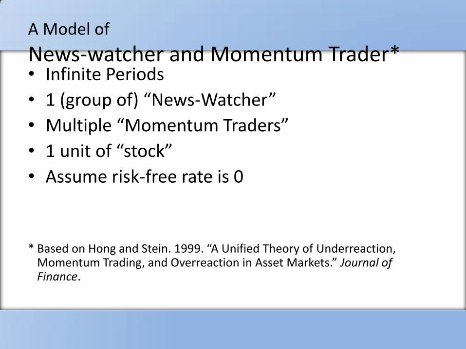
A Model of

News-watcher and Momentum Trader* • Infinite Periods

• 1 (group of) “News-Watcher”

• Multiple “Momentum Traders”

• 1 unit of “stock”

• Assume risk-free rate is 0

* Based on Hong and Stein. 1999. “A Unified Theory of Underreaction,

Momentum Trading, and Overreaction in Asset Markets.” Journal of Finance.

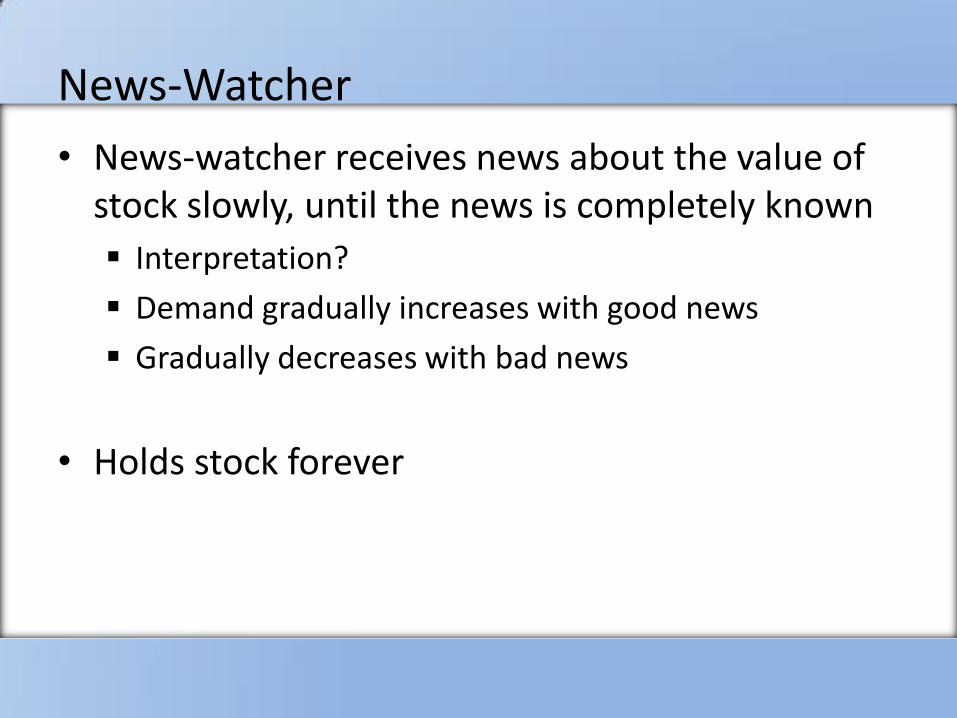
News-Watcher

• News-watcher receives news about the value of stock slowly, until the news is completely known

Interpretation?

Demand gradually increases with good news

Gradually decreases with bad news

• Holds stock forever

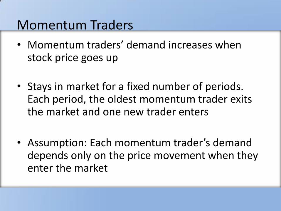
Momentum Traders

• Momentum traders’ demand increases when stock price goes up

• Stays in market for a fixed number of periods. Each period, the oldest momentum trader exits the market and one new trader enters

• Assumption: Each momentum trader’s demand depends only on the price movement when they enter the market

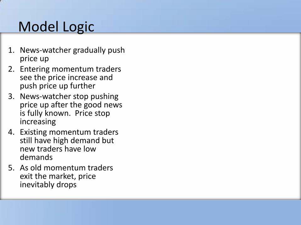
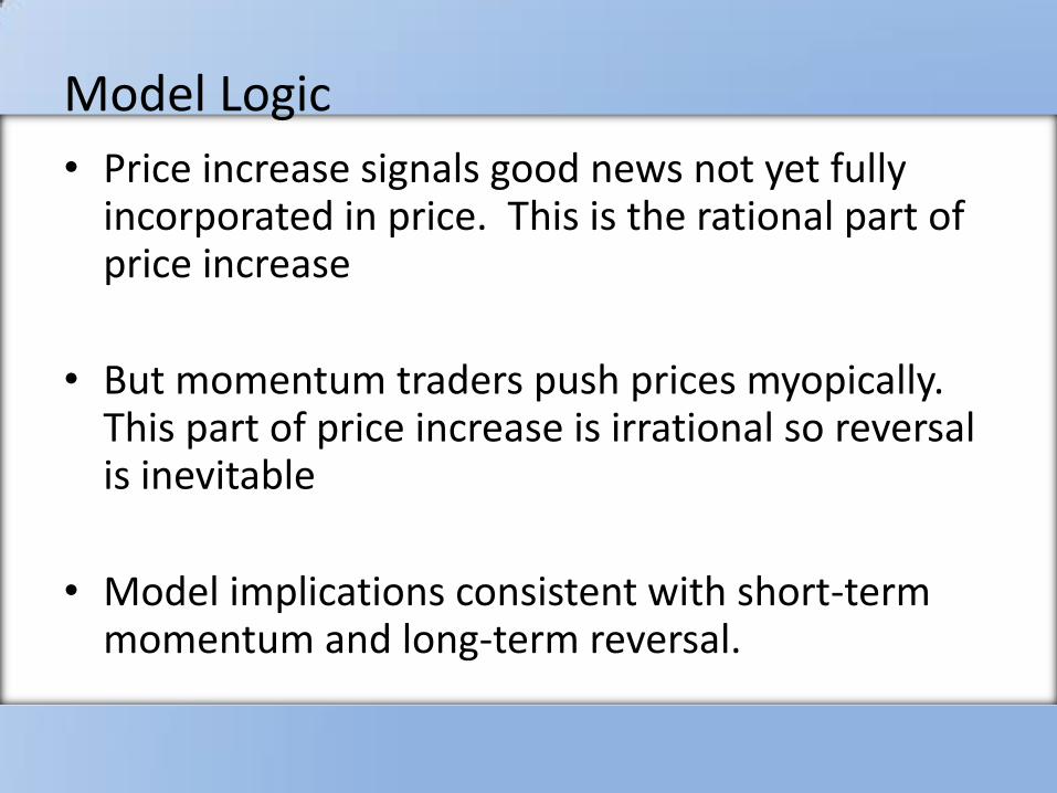
Model Logic

Suppose a good news is gradually spreading 1. News-watcher gradually push price up

2. Entering momentum traders see the price increase and push price up further

3. News-watcher stop pushing price up after the good news is fully known. Price stop increasing

4. Existing momentum traders still have high demand but new traders have low demands

5. As old momentum traders exit the market, price inevitably drops

Model Logic

1. News-watcher gradually push price up

2. Entering momentum traders see the price increase and push price up further

3. News-watcher stop pushing price up after the good news is fully known. Price stop increasing

4. Existing momentum traders still have high demand but new traders have low demands

5. As old momentum traders exit the market, price inevitably drops

Model Logic

• Price increase signals good news not yet fully incorporated in price. This is the rational part of price increase

• But momentum traders push prices myopically. This part of price increase is irrational so reversal is inevitable

• Model implications consistent with short-term momentum and long-term reversal.

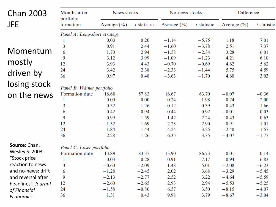
Chan 2003 JFE

Momentum mostly driven by losing stock on the news

Source: Chan, Wesley S. 2003. “Stock price reaction to news and no-news: drift and reversal after headlines”, Journal of Financial Economics

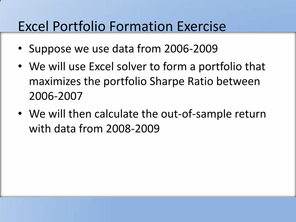
Excel Portfolio Formation Exercise

• Suppose we use data from 2006-2009

• We will use Excel solver to form a portfolio that maximizes the portfolio Sharpe Ratio between 2006-2007

• We will then calculate the out-of-sample return with data from 2008-2009