Economic evaluation of transportation projects: An ... · Economic evaluation of transportation...

공간경제연구실 Spat ia l Economics Laboratory h t t p : / / s p e c o n . s n u . a c . k r

Economic evaluation of transportation projects: An application of Financial Computable General Equilibrium

model

ERCI/ERCD Internal Seminars on Asian Economic Integration Report 2018

December 15, 2017

Euijune Kim

Geoffrey J. D. Hewings

Hidayat Amir

Seoul National University

[email protected]

Asian Development Bank, Manila, Philippine

Ⅰ. Background

Ⅲ. Simulation

Contents

Ⅱ. Model

Ⅳ. Summary

Spatial Economics Laboratory Seoul National University -3-

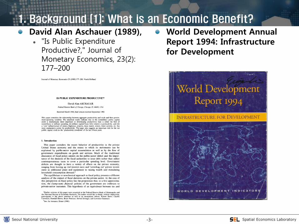
1. Background (1): What is an Economic Benefit? David Alan Aschauer (1989), "Is Public Expenditure

Productive?," Journal of Monetary Economics, 23(2): 177–200

World Development Annual Report 1994: Infrastructure for Development


1. Background (2): Classification of Benefits

Direct and indirect effects in terms of ‘who gets benefits’

Direct effects Decrease in transport time for user (driver) and in operation cost per

passenger Improvement of transport service

Indirect effects Production and agglomeration economies Location and migration (commuting) Communication, and knowledge spill-over effect

Temporary and permanent effects in terms of benefit duration

Temporary (flow, construction or short run) effects To be generated during construction period

Permanent (stock, operation or long run) effects To be generated by consuming infrastructure services: transport cost and

time benefits for people and freight Backward effect of the infrastructure expenditures (excluding construction) Re-location of people and firms


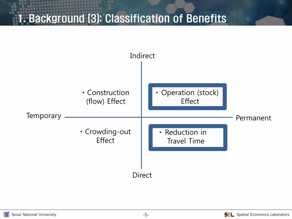
1. Background (3): Classification of Benefits

Temporary Permanent

Direct

Indirect

• Construction (flow) Effect

• Operation (stock) Effect

• Crowding-out Effect

• Reduction in Travel Time


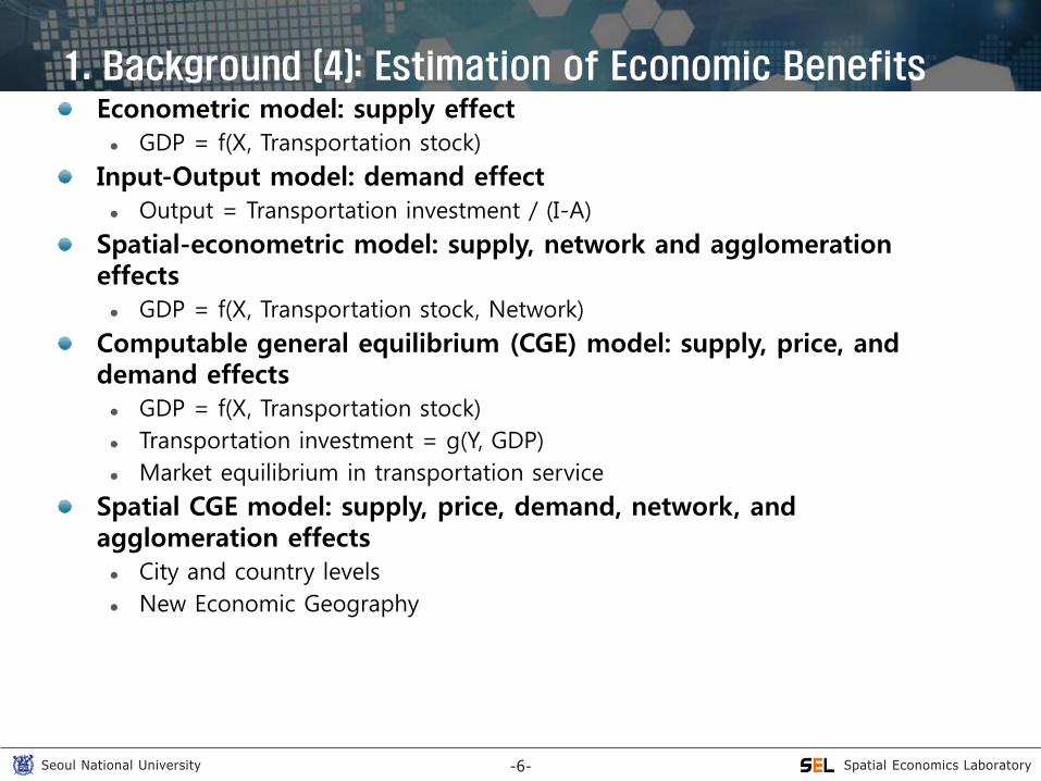
1. Background (4): Estimation of Economic Benefits Econometric model: supply effect

GDP = f(X, Transportation stock)

Input-Output model: demand effect

Output = Transportation investment / (I-A)

Spatial-econometric model: supply, network and agglomeration effects

GDP = f(X, Transportation stock, Network)

Computable general equilibrium (CGE) model: supply, price, and demand effects

GDP = f(X, Transportation stock)

Transportation investment = g(Y, GDP)

Market equilibrium in transportation service

Spatial CGE model: supply, price, demand, network, and agglomeration effects

City and country levels

New Economic Geography


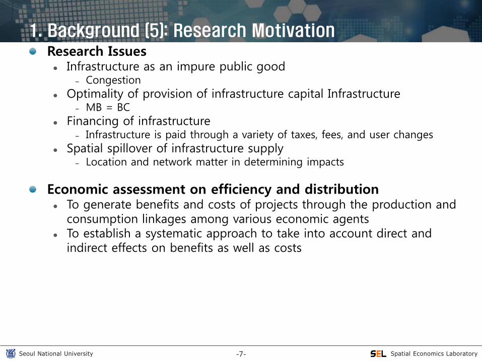
1. Background (5): Research Motivation Research Issues Infrastructure as an impure public good

Congestion

Optimality of provision of infrastructure capital Infrastructure MB = BC

Financing of infrastructure Infrastructure is paid through a variety of taxes, fees, and user changes

Spatial spillover of infrastructure supply Location and network matter in determining impacts

Economic assessment on efficiency and distribution To generate benefits and costs of projects through the production and

consumption linkages among various economic agents To establish a systematic approach to take into account direct and

indirect effects on benefits as well as costs


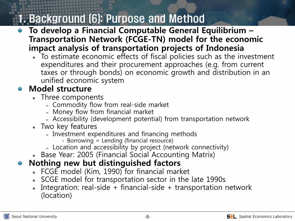
1. Background (6): Purpose and Method To develop a Financial Computable General Equilibrium – Transportation Network (FCGE-TN) model for the economic impact analysis of transportation projects of Indonesia To estimate economic effects of fiscal policies such as the investment

expenditures and their procurement approaches (e.g. from current taxes or through bonds) on economic growth and distribution in an unified economic system

Model structure Three components

Commodity flow from real-side market Money flow from financial market Accessibility (development potential) from transportation network

Two key features Investment expenditures and financing methods

- Borrowing = Lending (financial resource) Location and accessibility by project (network connectivity)

Base Year: 2005 (Financial Social Accounting Matrix) Nothing new but distinguished factors FCGE model (Kim, 1990) for financial market SCGE model for transportation sector in the late 1990s Integration: real-side + financial-side + transportation network

(location)


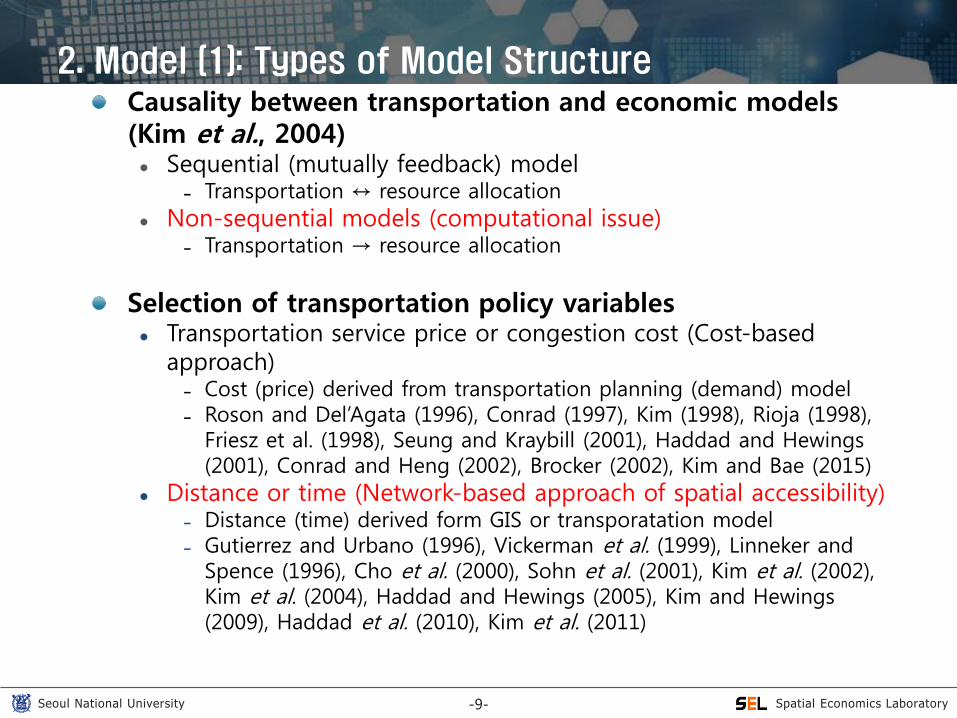
2. Model (1): Types of Model Structure Causality between transportation and economic models (Kim et al., 2004) Sequential (mutually feedback) model

Transportation ↔ resource allocation

Non-sequential models (computational issue) Transportation → resource allocation

Selection of transportation policy variables Transportation service price or congestion cost (Cost-based

approach) Cost (price) derived from transportation planning (demand) model Roson and Del’Agata (1996), Conrad (1997), Kim (1998), Rioja (1998),

Friesz et al. (1998), Seung and Kraybill (2001), Haddad and Hewings (2001), Conrad and Heng (2002), Brocker (2002), Kim and Bae (2015)

Distance or time (Network-based approach of spatial accessibility) Distance (time) derived form GIS or transporatation model Gutierrez and Urbano (1996), Vickerman et al. (1999), Linneker and

Spence (1996), Cho et al. (2000), Sohn et al. (2001), Kim et al. (2002), Kim et al. (2004), Haddad and Hewings (2005), Kim and Hewings (2009), Haddad et al. (2010), Kim et al. (2011)


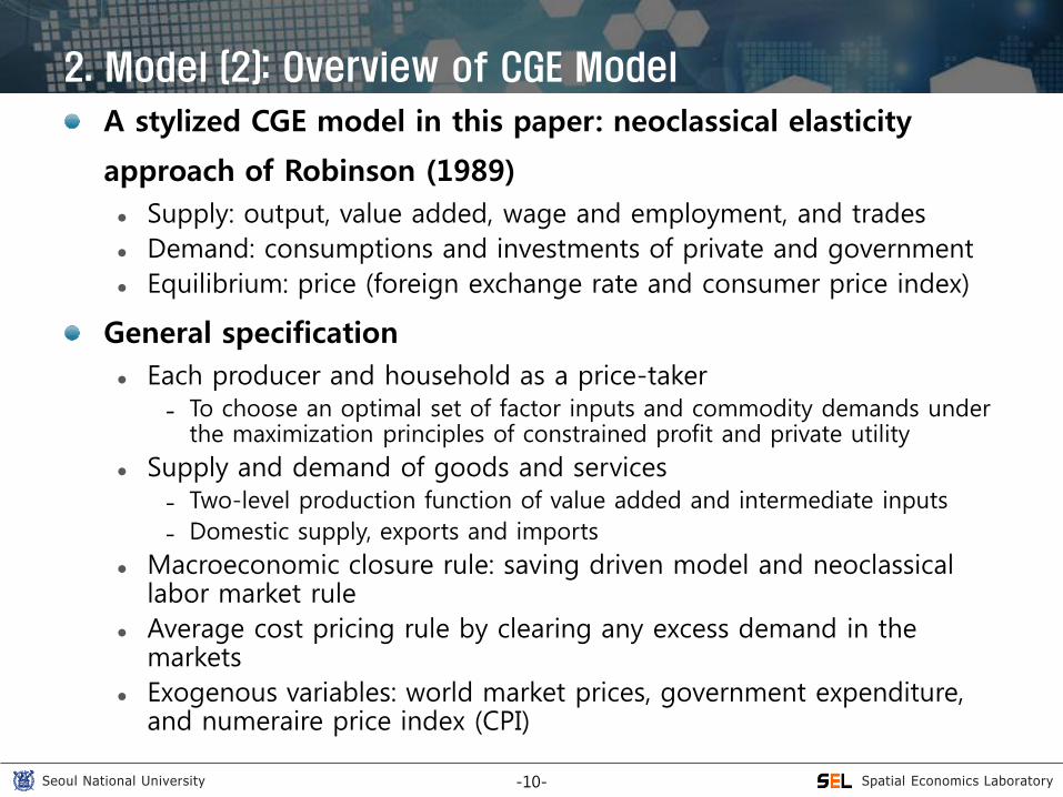
2. Model (2): Overview of CGE Model

A stylized CGE model in this paper: neoclassical elasticity

approach of Robinson (1989)

Supply: output, value added, wage and employment, and trades

Demand: consumptions and investments of private and government

Equilibrium: price (foreign exchange rate and consumer price index)

General specification

Each producer and household as a price-taker To choose an optimal set of factor inputs and commodity demands under

the maximization principles of constrained profit and private utility

Supply and demand of goods and services Two-level production function of value added and intermediate inputs

Domestic supply, exports and imports

Macroeconomic closure rule: saving driven model and neoclassical labor market rule

Average cost pricing rule by clearing any excess demand in the markets

Exogenous variables: world market prices, government expenditure, and numeraire price index (CPI)


2. Model (3): Two-Sector Model

S

D Q

P

Q*

P*

Commodity

Factor Inputs (Labor, Capital, and Land)

Consumer’s

Utility Max.

Producer’s

Profit Max.

MAX

Demand

Demand

Supply

Supply


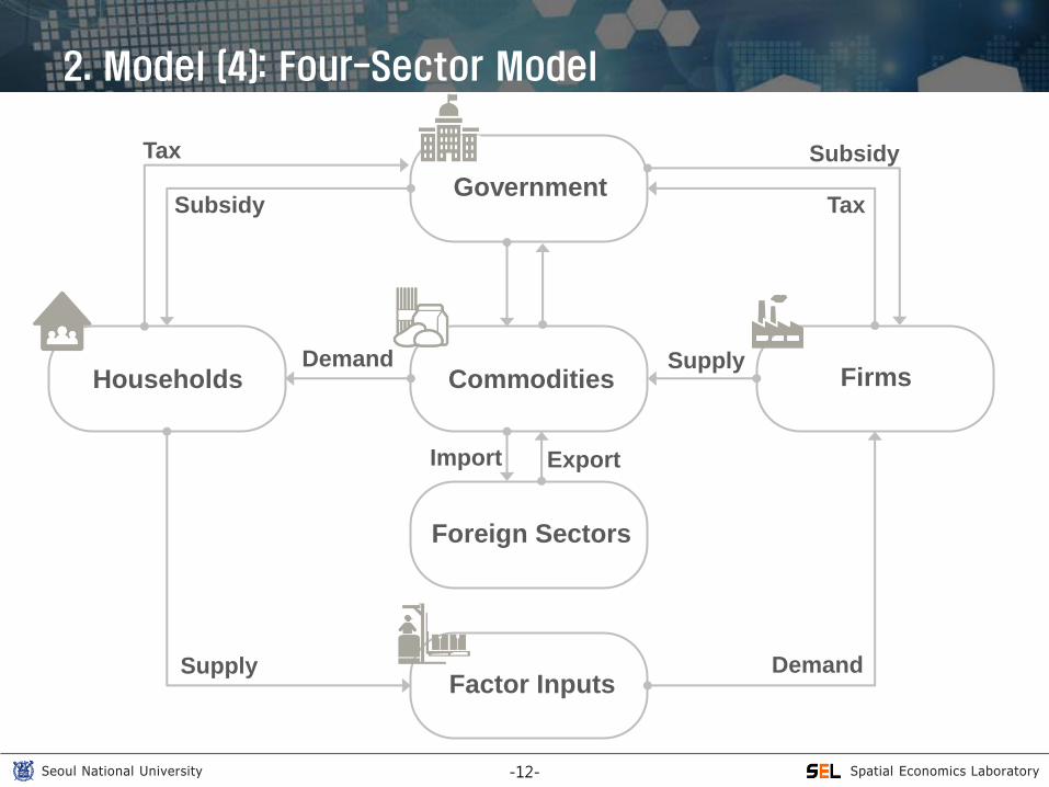
Foreign Sectors

Government

Factor Inputs

Firms Households Commodities

Import Export

Subsidy

Tax

Tax

Subsidy

Demand

Demand

Supply

Supply

2. Model (4): Four-Sector Model


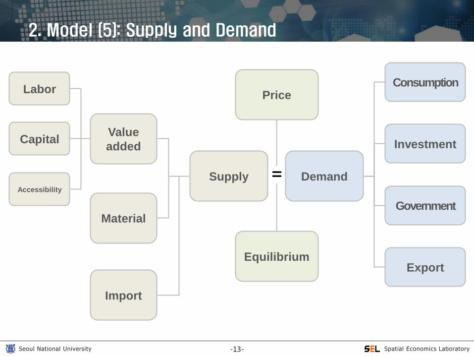
Capital

Labor

Accessibility

Value

added

Material

Import

Supply Demand

Price

Equilibrium

Consumption

Investment

Government

Export

=

2. Model (5): Supply and Demand


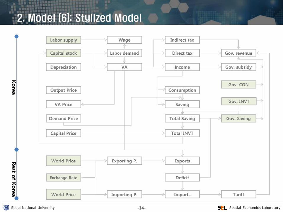
Labor supply

Capital stock

Depreciation

Output Price

VA Price

Demand Price

Capital Price

World Price

Exchange Rate

Wage

Labor demand

VA

Exporting P.

Indirect tax

Direct tax

Income

Consumption

Saving

Total Saving

Total INVT

Exports

Deficit

Gov. revenue

Gov. subsidy

Gov. CON

Gov. INVT

Gov. Saving

World Price Importing P. Imports Tariff

Rest o

f Kore

a

Kore

a

2. Model (6): Stylized Model


2. Model (7): Sectoral Classification

Seven institutions (households, government and firms) Central bank, Company and Government Rural Poor, Rural High, Urban Poor and Urban High

Nine industrial sectors Agriculture, Mining, Manufacturing, Utility, Construction, Trade-Hotel-

Restaurant, Transportation-Communication, Finance, and Other Sector

Three financial instruments for infrastructure investments (Bank of Indonesia) Government revenues National bond Composite Financial Asset (Cadangan Valas Pemerintah, Cartel, Giro,

Saving, Deposito, Certificate of Bank Indonesia, Other Long-Term Securities, Short-Term Securities, Working Capital Credit, Investment Credit, Consumption Credit, Non-Bank Credit, Trade Credit, Capital Stock and Inclusion, Insurance Reverse and Pension)


2. Model (8): Linkages

Extensions to financial market

Linkage between total factor productivity and accessibility (infrastructure networking) in manufacturing sector

Supply-demand-price mechanism of financial instruments (assets)

Inclusion of property incomes and costs for economic agents

Flows of financial income among economic agents

What we need for the impact analysis

Amounts and period of infrastructure investments

Location (connectivity to the network)

Financing method: tax revenues, national bonds and private funds


2. Model (9): Model Comparison


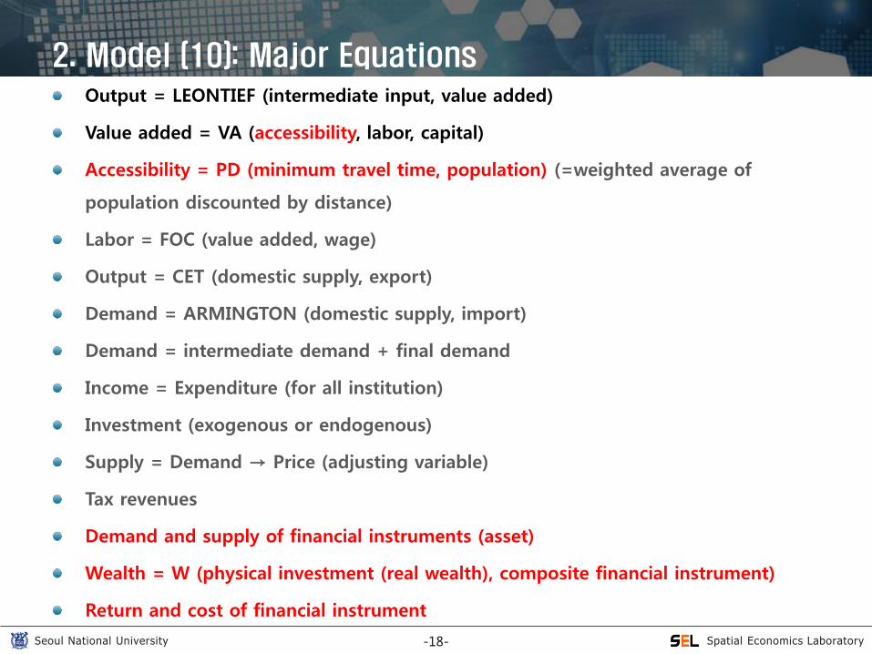
2. Model (10): Major Equations Output = LEONTIEF (intermediate input, value added)

Value added = VA (accessibility, labor, capital)

Accessibility = PD (minimum travel time, population) (=weighted average of

population discounted by distance)

Labor = FOC (value added, wage)

Output = CET (domestic supply, export)

Demand = ARMINGTON (domestic supply, import)

Demand = intermediate demand + final demand

Income = Expenditure (for all institution)

Investment (exogenous or endogenous)

Supply = Demand → Price (adjusting variable)

Tax revenues

Demand and supply of financial instruments (asset)

Wealth = W (physical investment (real wealth), composite financial instrument)

Return and cost of financial instrument


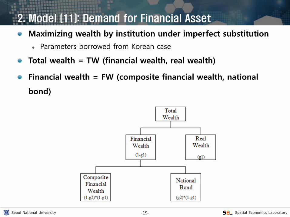
2. Model (11): Demand for Financial Asset

Maximizing wealth by institution under imperfect substitution

Parameters borrowed from Korean case

Total wealth = TW (financial wealth, real wealth)

Financial wealth = FW (composite financial wealth, national

bond)


2. Model (12): FCGE-TN Model Structure


2. Model (13): FSAM (Bank of Indonesia)


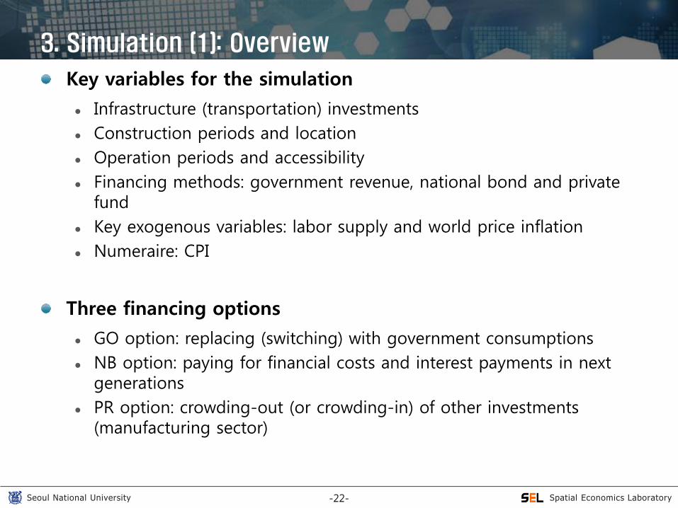
3. Simulation (1): Overview

Key variables for the simulation

Infrastructure (transportation) investments

Construction periods and location

Operation periods and accessibility

Financing methods: government revenue, national bond and private fund

Key exogenous variables: labor supply and world price inflation

Numeraire: CPI

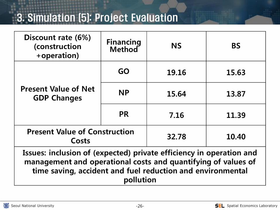
Three financing options

GO option: replacing (switching) with government consumptions

NB option: paying for financial costs and interest payments in next generations

PR option: crowding-out (or crowding-in) of other investments (manufacturing sector)


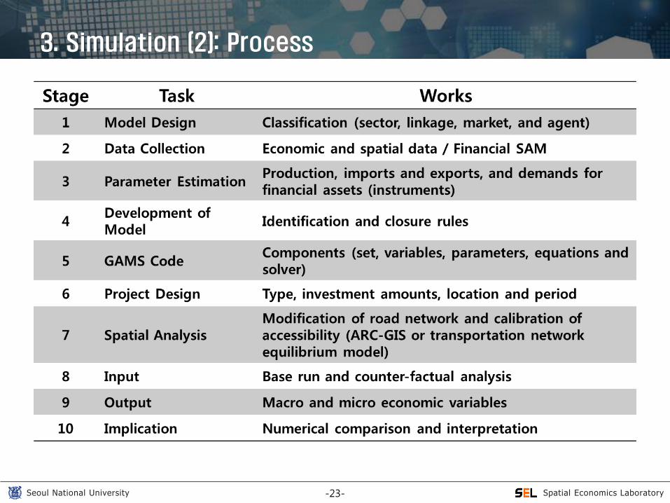
3. Simulation (2): Process


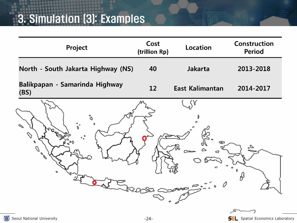
3. Simulation (3): Examples


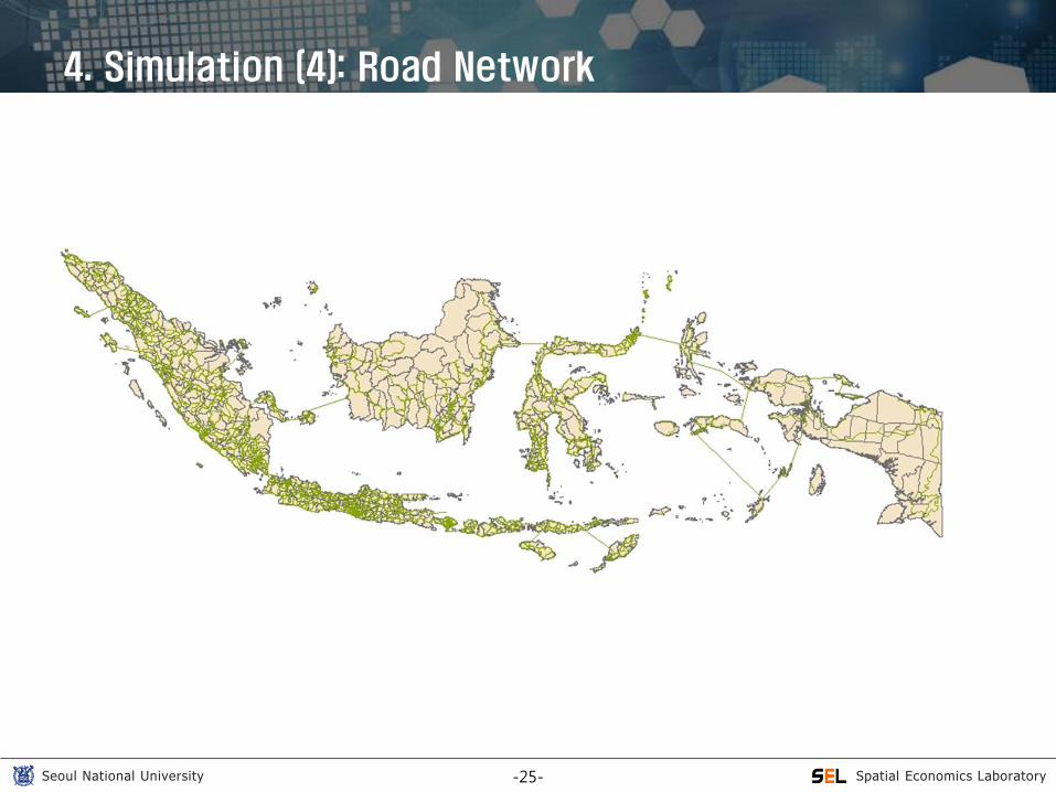
4. Simulation (4): Road Network


3. Simulation (5): Project Evaluation


4. Further Research Works

Summary

Positive impacts on the economic growth, but depending on the financing methods and location

Not substantial impact on the income distribution

Research issues

Data Consistency of FSAM with Real SAM

Classification of household groups (types of works and income sources)

Extension of transportation network: road and railroad

Direct effects (benefit): time savings and reductions in accidental and environmental costs

Spatial unit Decomposing accessibility into intra- and inter-islands

Infrastructure policies: seaport and airports

Migration

Operation efficiency by ownership BOT and privatization

Economic evaluation of transportation projects: An ... · Economic evaluation of transportation...

Documents

Transcript of Economic evaluation of transportation projects: An ... · Economic evaluation of transportation...