Ecological Statistics
53
-
Upload
gururaja-kv -
Category
Education
-
view
4.256 -
download
3
description
What we look at ecological statistics, descriptive and inductive statistics, biodiversity index, examples from Sharavathi river basin
Transcript of Ecological Statistics

Gururaja KVIISc, [email protected]
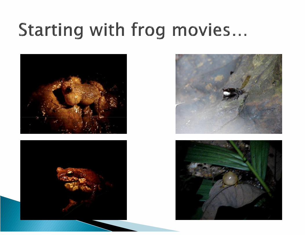


Systematic stratified random sampling Systematic stratified random sampling Night survey, from 2003 Night survey, from 2003 –– 2006, seasonal, 2006, seasonal,
search for all search for all Identify and record species, numbers etc.Identify and record species, numbers etc. Secondary data on Vegetation studies, RS and Secondary data on Vegetation studies, RS and Secondary data on Vegetation studies, RS and Secondary data on Vegetation studies, RS and
GISGIS Opportunistic observations also included for Opportunistic observations also included for
overall diversity in the regionoverall diversity in the region Shannon’s index (Shannon’s index (H’ = H’ = -- Σ pΣ pii lnln ppii)), , Simpson’s index (Simpson’s index (D = 1/ Σ pD = 1/ Σ pii
22))

Varieties of species (Species richness)Varieties of species (Species richness) Abundance of species (#Abundance of species (#indvidualsindviduals/man hour /man hour
search)search) Derived data (Endemics, Endemic abundance)Derived data (Endemics, Endemic abundance) Secondary source (IUCN red list)Secondary source (IUCN red list) Secondary source (IUCN red list)Secondary source (IUCN red list) Percent Evergreens, rainfall, percent Percent Evergreens, rainfall, percent landuseslanduses, ,
forest fragmentation data, forest fragmentation data,

Sampling sites
Longitude (°E) Latitude(°N) Altitude (m)
1 75.0896 13.773 584
2 75.0804 13.8532 586
3 74.8839 13.9269 580
4 74.7268 13.965 563
5 75.1055 13.9735 602
6 74.8428 13.9786 598
7 75.1084 14.0209 559
8 75.1245 14.0418 557
9 75.073 14.0831 680
10 75.04 14.058 596
11 75.109 13.7379 696
12…


Euphlyctis cyanophlyctis 11 1 1Euphlyctis hexadactylus 1Hoplobatrachus tigerinus 1 1 2 1 1Indirana beddomii 1Indirana semipalmatus 1 5 1 2Fejervarya granosa 1Fejervarya caperata 4 1 5 2 3 3 4Minervarya sahyadris 1Minervarya sahyadris 1Micrixalus fuscus 6Micrixalus saxicola 2Nyctibatrachus aliciae 2 3Nyctibatrachus major 15Philautus sp1 1 2Philautus amboli 2 6 37 6 4 3 7 8Philautus sp2 2 3 1 1 1Philautus tuberohumerus 3 2 2 1Polypedates maculatus 1
List is incomplete…species wise..as well as site wise
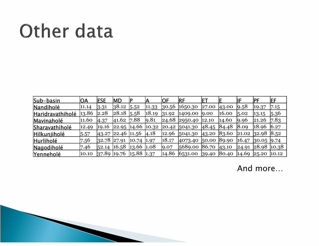
Sub-basin OA ESE MD P A OF RF ET E IF PF EFNandiholé 11.14 3.31 38.12 5.52 11.33 30.56 1650.30 27.00 43.00 9.58 19.37 7.15
Haridravathiholé 13.86 2.28 28.18 5.58 18.19 31.92 1409.00 9.00 16.00 5.02 13.15 5.36
Mavinaholé 11.60 4.37 41.62 7.88 9.81 24.68 2950.40 12.10 14.60 9.96 21.26 7.83MavinaholéSharavathiholé 12.49 19.16 22.95 14.66 10.32 20.42 5041.30 48.45 84.48 8.09 18.96 6.27
Hilkunjiholé 5.57 43.27 22.46 11.56 4.18 12.96 5041.30 43.20 83.60 21.02 32.98 8.52
Hurliholé 7.56 32.78 27.91 10.74 1.97 18.17 4073.40 50.00 89.90 16.47 30.05 9.74
Nagodiholé 7.46 52.14 16.58 13.66 1.08 9.07 5689.00 86.70 43.10 24.91 28.98 10.38
Yenneholé 10.10 37.89 19.76 15.88 1.37 14.86 6531.00 39.40 80.40 14.69 25.20 10.12
And more…

Back to the questions asked Statistical application…find out the
relationship (among variables and between amphibian diversity and these variables)
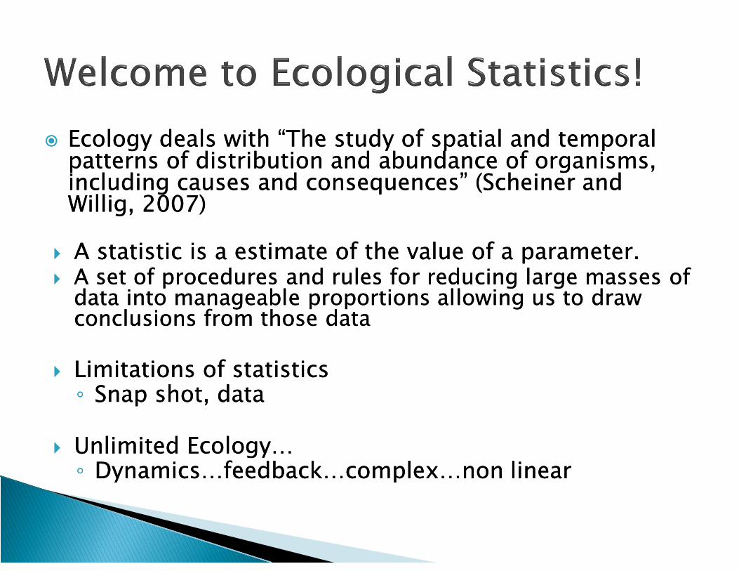
Ecology deals with “The study of spatial and temporal Ecology deals with “The study of spatial and temporal patterns of distribution and abundance of organisms, patterns of distribution and abundance of organisms, including causes and consequences” (including causes and consequences” (ScheinerScheiner and and WilligWillig, 2007), 2007)
A statistic is a estimate of the value of a parameter. A statistic is a estimate of the value of a parameter. A set of procedures and rules for reducing large masses of A set of procedures and rules for reducing large masses of
data into manageable proportions allowing us to draw data into manageable proportions allowing us to draw A set of procedures and rules for reducing large masses of A set of procedures and rules for reducing large masses of
data into manageable proportions allowing us to draw data into manageable proportions allowing us to draw conclusions from those dataconclusions from those data
Limitations of statisticsLimitations of statistics◦◦ Snap shot, data Snap shot, data
Unlimited Ecology…Unlimited Ecology…◦◦ Dynamics…feedback…complex…non linearDynamics…feedback…complex…non linear

Part I◦ Framing a good question?◦ Setting the objectives?◦ Sampling design, Replication, Randomnization
Part II◦ Parameteric vs Non parametric◦ Goodness of fit◦ Goodness of fit◦ Measuring central tendency◦ Hypothesis testing◦ Measuring relationships
Part III◦ Measuring biodiversity◦ Ordination, Multivariate analysis◦ Spatial analysis

Measurement – assignment of a number to something
Data – information on species, variable, parameter
Sample – Small portion of a population Sample – Small portion of a population Population – all possible units of a given area Variable – Varies with the influence of other. Parameter – A measurable unit (eg.
Temperature, pH)
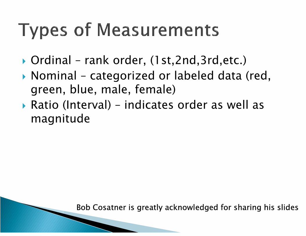
Ordinal – rank order, (1st,2nd,3rd,etc.) Nominal – categorized or labeled data (red,
green, blue, male, female) Ratio (Interval) – indicates order as well as
magnitudemagnitude
Bob Cosatner is greatly acknowledged for sharing his slides
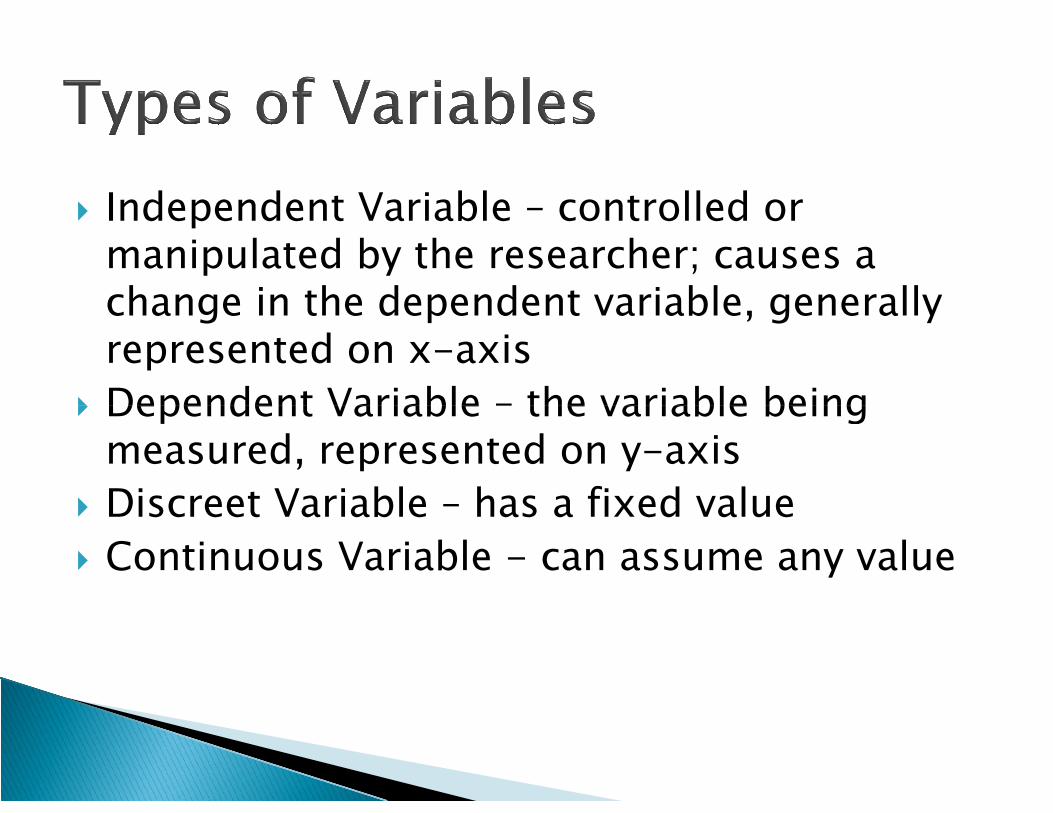
Independent Variable – controlled or manipulated by the researcher; causes a change in the dependent variable, generally represented on x-axis
Dependent Variable – the variable being Dependent Variable – the variable being measured, represented on y-axis
Discreet Variable – has a fixed value Continuous Variable - can assume any value

Mean (average) Median (middle) Mode (most frequent)


Variance standard deviation standard error

Sample variance is summation of square of deviance from each data point divided by n-1, In excel it is given by VAR(data)


Earlier part was descriptive statistics! Null (H0) vs alternate hypothesis(H1) Null Hypothesis Statistical hypotheses
usually assume no relationship between variables. Eg. there is no association between variables. Eg. there is no association between eye color and eyesight.
No change Change
Change detected Reject (1) Accept
No change detected
Accept Reject (II)


Tree height1
(cm)
Tree height 2
(cm)1 1014 8642 684 6363 810 7084 990 786 0
200
400
600
800
1000
1200
1400
5 840 6006 978 13207 1002 7508 1110 5949 800 750
0 2 4 6 8 10
Tree height1 Tree height 2

Distribution free analysis Comparison between observed data vs
expected data Generally for qualitative data and categorical
datadata Chi square = sum (OE)2/E

At df 8, 818.1, p<0.001 Null hypothesis rejected There is a difference between observed vs
expected value in tree height

Relationship between dependent and independent variables
Quantification of relationships Pearsons correlation coefficient (r)
Simple scatter plot will explain r=0.255, R=0.0652 y = 0.4161x + 398.28
R² = 0.0652
0
200
400
600
800
1000
1200
1400
0 200 400 600 800 1000 1200

t=1.562, p>0.05
400
600
800
1000
1200
1400
1600
1800
Treeheight1Treeheight2
Y
1 2 3 4 5 6 7 8 90
200
400
Treeheight1 Treeheight2N 9 9Min 684 594Max 1110 1320Sum 8228 7008Mean 914.222 778.667Std. error 45.3719 73.9174Variance 18527.4 49174Stand. dev 136.116 221.752Median 978 75025 prcntil 805 61875 prcntil 1008 825
Tre
ehei
g
Tre
ehei
g
600
700
800
900
1000
1100
1200
1300
Y
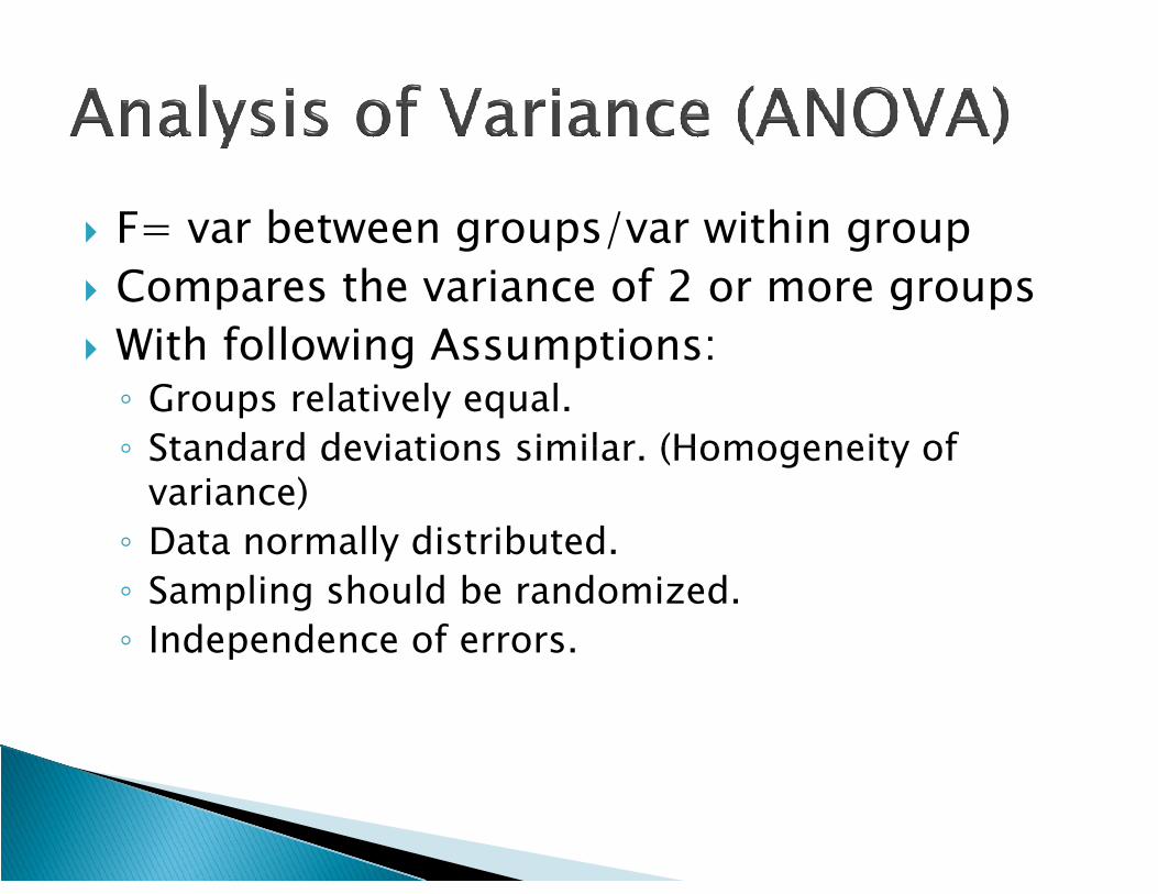
F= var between groups/var within group Compares the variance of 2 or more groups With following Assumptions:◦ Groups relatively equal.◦ Standard deviations similar. (Homogeneity of ◦ Standard deviations similar. (Homogeneity of
variance)◦ Data normally distributed.◦ Sampling should be randomized.◦ Independence of errors.


•• 42 species, 7 families 42 species, 7 families
•• 27 endemic to Western Ghats (64%) 27 endemic to Western Ghats (64%) •• 12 vulnerable12 vulnerable
•• 17 near threatened 17 near threatened
•• NandiholNandiholéé least richness, abundance least richness, abundance •• YenneholYenneholéé highest highest •• YenneholYenneholéé highest highest Su b-ba sin Rich n ess A bu nd. Endem ic En .A bu Non -en d. Non .A bu Sim pson Sh a nn on
Na n di 1 0 3 6 4 1 2 6 2 4 5 .4 5 6 1 .9 6 3
Ha r idr a v a th i 1 4 4 9 6 2 8 8 2 1 8 .7 4 7 2 .3 5 6
Ma v in h ole 1 4 4 8 8 2 8 6 2 0 7 .6 2 9 2 .2 9 8
Sh a r a v a th i 1 4 3 3 9 2 7 5 6 7 .3 1 6 2 .2 9 8
Hilku n ji 2 0 4 8 1 1 3 1 9 1 7 1 0 .1 2 8 2 .6 5 3
Na g odi 1 8 5 9 1 1 4 5 7 1 4 7 .5 4 8 2 .4 3 6
Hu r li 1 5 3 8 9 2 6 6 1 2 1 1 .1 00 2 .5 4 4
Yen n e 2 2 6 6 1 3 3 5 9 3 1 1 3 .2 9 9 2 .8 07
Richness Abundance
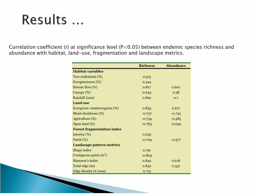
Tree endemism (%) 0.513
Evergreenness (%) 0.544
Stream flow (%) 0.817 0.607
Canopy (%) 0.643 0.58
Rainfall (mm) 0.892 0.7
Habitat variables
Correlation coefficient (r) at significance level (P<0.05) between endemic species richness and abundance with habitat, land-use, fragmentation and landscape metrics.
Rainfall (mm) 0.892 0.7
Evergreen–semievergreen (%) 0.853 0.617
Moist deciduous (%) -0.737 -0.735
Agriculture (%) -0.734 -0.585
Open land (%) -0.783 -0.659
Interior (%) 0.635
Patch (%) -0.709 -0.577
Shape index 0.791
Contiguous patch (m2) -0.809
Shannon’s index 0.842 0.618
Total edge (m) 0.832 0.551
Edge density (#/area) 0.715
Land-use
Forest fragmentation index
Landscape pattern metrics

1 2 3 4 5 6 7 8 9 10 11 12 13 14 15 16
2 0.9 8 5
3 0.8 1 2 0.8 5 5
4 0.6 7 5 0.7 0 4 0.6 2 8
5 0.7 9 1 0.8 2 4 0.9 7 3 0.7 4 9
6 0.8 5 8 0.8 7 8 0.9 6 5 0.7 7 1 0.9 9 2
7 -0.6 -0.7 -0.8 -0.8 1 -0.8 3 -0.8
8 -0.6 7 -0.7 -0.9 2 -0.8 9 -0.8 6 0.6 8 9
Correlation coefficient (r) at significance level (P<0.05) among the environmental descriptors.
8 -0.6 7 -0.7 -0.9 2 -0.8 9 -0.8 6 0.6 8 9
9 -0.7 -0.7 3 -0.8 7 -0.7 8 -0.9 3 -0.9 2 0.7 5 5 0.8 4 5
10 0.7 01 0.6 9 5 0.8 06 0.5 9 6 0.8 4 1 0 .8 4 7 -0.5 4 -0.8 7 -0.9 4
11 0.7 3 6 0.7 0 6 0.7 9 9 0.5 2 6 0.8 2 8 0 .8 4 9 -0.8 -0.8 9 0.9 6 2
12 -0.6 7 -0.6 9 -0.8 6 -0.6 4 -0.9 -0.8 8 0.6 5 2 0.8 9 1 0.9 7 6 -0.9 8 -0.9 3
13 0.8 7 3 0.9 0.9 07 0.7 6 2 0.9 2 5 0 .9 5 2 -0.7 6 -0.7 -0.8 2 0.7 1 1 0.7 6 5 -0.7 5
14 -0.8 7 -0.8 9 -0.9 1 -0.7 6 -0.9 2 -0.9 4 0.7 8 2 0.6 9 0.7 6 1 -0.6 3 -0.6 8 0 .6 8 7 -0.9 8
15 0.8 3 1 0.8 6 4 0.9 2 3 0.7 5 4 0.9 3 4 0 .9 4 4 -0.8 2 -0.7 2 -0.7 7 0.6 3 0.6 6 5 -0.7 0.9 6 5 -0.9 9
16 0.8 1 2 0.8 5 8 0.8 9 6 0.7 2 2 0.9 07 0 .9 2 1 -0.8 -0.6 8 -0.7 5 0.6 1 4 0.6 6 1 -0.6 7 0.9 7 7 -0.9 7 0.9 6 9
17 0.9 3 5 0.9 4 3 0.9 06 0.7 7 0.9 1 7 0 .9 5 6 -0.7 1 -0.7 2 -0.8 4 0.7 7 0.8 1 4 -0.7 9 0.9 7 8 -0.9 6 0.9 4 1 0.9 2 1
1. Tree endemism; 2. Evergreenness; 3. Stream flow; 4. Canopy; 5. Rainfall; 6. Evergreen-semievergreen; 7. Moistdeciduous; 8. Agriculture; 9. Open land; 10. Interior; 11. Perforated; 12. Patch; 13. Shape index; 14. Contiguous patch; 15. Shannon’s index; 16. Total edge; 17. Edge density

0.3
1.0
1.6
Tree endemism
Evergreenness
Agriculture field
Open field
Patch forest
Landscape shape index
Shannon’s patch index
Total edge forest
4
5
0.3
1.0
1.6
Tree endemism
Evergreenness
Agriculture field
Open field
Patch forest
Landscape shape index
Shannon’s patch index
Total edge forest
4
5
Axi
s 2
Axis 1
-0.3
-1.0
-1.6
-0.3-1.0-1.6 0.3 1.0 1.6
Stream flowRain fall Evergreen-Semi-evergreen
Interior forest
Contiguous forest
Vector scaling: 2.50
6
71
2
3
5
8Axi
s 2
Axis 1
-0.3
-1.0
-1.6
-0.3-1.0-1.6 0.3 1.0 1.6
Stream flowRain fall Evergreen-Semi-evergreen
Interior forest
Contiguous forest
Vector scaling: 2.50
6
71
2
3
5
8
1. Nandihole, 2. Haridravathi, 3. Mavinhole, 4. Sharavathi, 5. Hilkunji, 6. Hurli, 7. Nagodi and 8. Yennehole

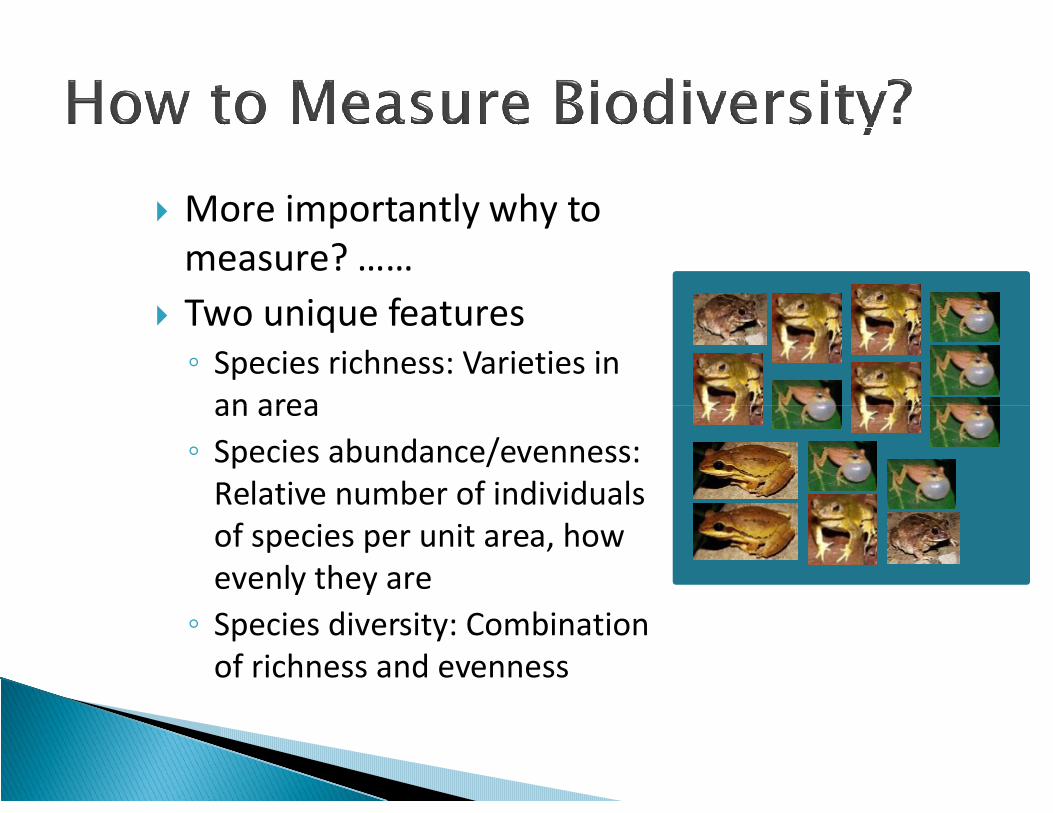
More importantly why to measure? ……
Two unique features◦ Species richness: Varieties in
an areaan area◦ Species abundance/evenness:
Relative number of individuals of species per unit area, how evenly they are◦ Species diversity: Combination
of richness and evenness

Alpha (α) – Number of species in a given habitat or natural community
Beta (β) – Degree of variation in diversity from patch to patch
Gamma and Epsilon (γ and ε) –Species richness of a range of habitats in a geographical area habitats in a geographical area (Island)/region. Consequence of Alpha and Beta diversity
α and γ scalar, only magnitude, βvector both scalar and vector ©Van dyke, 2003
Distribution basedDistribution based Parametric – Assumes normal distribution, eg. log-normal, etc. Non-parametric – Distribution free, Shannon’s, Simpson’s, etc.
15
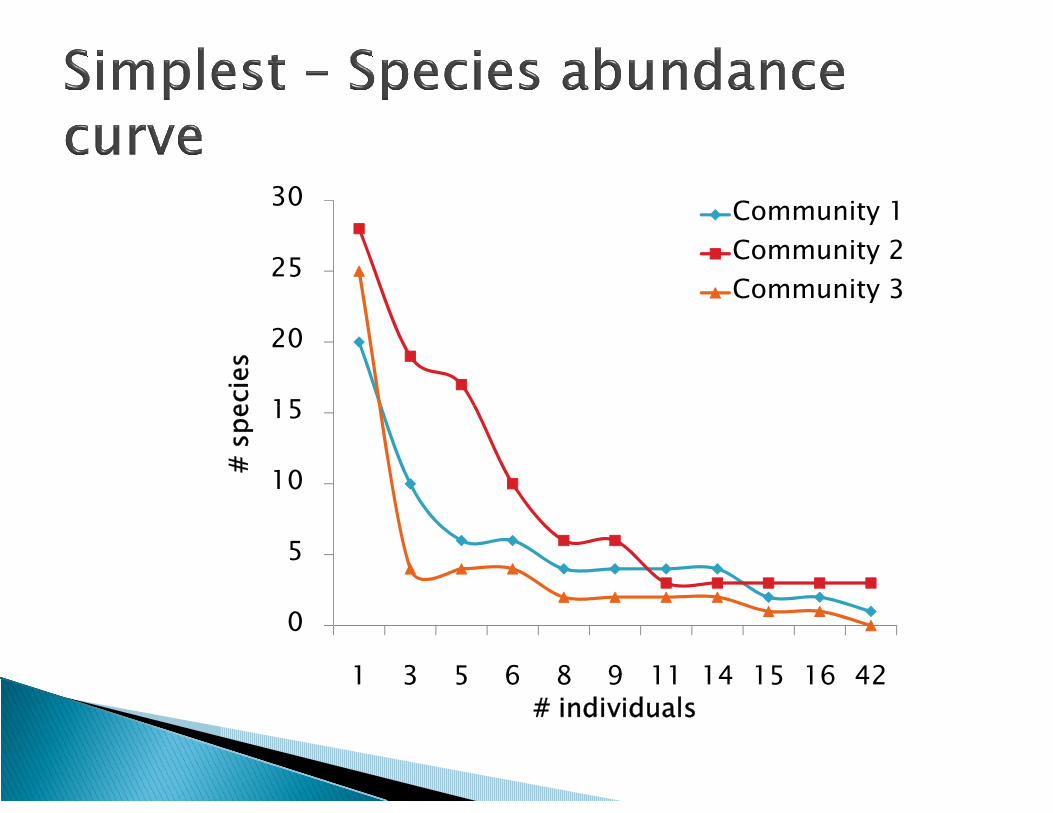
20
25
30
# s
peci
esCommunity 1
Community 2
Community 3
0
5
10
15
1 3 5 6 8 9 11 14 15 16 42
# s
peci
es
# individuals
Rel
ativ
e A
bu
nd
ance
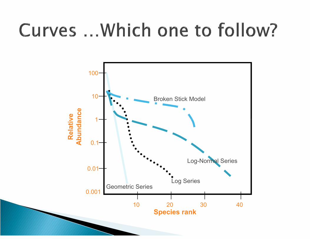
100
10
1
Broken Stick Model
Rel
ativ
e A
bu
nd
ance
1
0.1
0.01
0.001
10 20 30 40
Geometric SeriesLog Series
Log-Normal Series
Species rank
1500
2000
2500
3000A
bundan
ceUrban
Rural
Scrub
Rel
ativ
e A
bu
nd
ance
100
10
1
Broken Stick Model
0
500
1000
1500
1 2 3 4 5 6 7 8 9 10
Ab
undan
ce
Species rank
Rel
ativ
e A
bu
nd
ance
0.1
0.01
0.001
10 20 30 40
Geometric Series
Log-Normal Series
Species rank
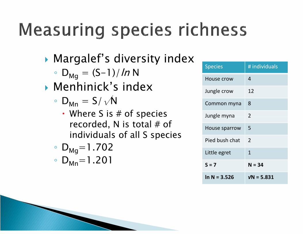
Margalef’s diversity index◦ DMg = (S-1)/ln N
Menhinick’s index◦ DMn = S/√N Where S is # of species
Species # individuals
House crow 4
Jungle crow 12
Common myna 8
Jungle myna 2 Where S is # of species recorded, N is total # of individuals of all S species
◦ DMg=1.702◦ DMn=1.201
Jungle myna 2
House sparrow 5
Pied bush chat 2
Little egret 1
S = 7 N = 34
ln N = 3.526 √N = 5.831

Heterogeneity Indices◦ Consider both evenness and richness◦ Species abundance models only consider evenness
No assumptions made about species abundance distributionsabundance distributions◦ Cause of distribution◦ Shape of curve
Non-parametric◦ Free of assumptions of normality

Information Theory◦ Diversity (or information) of a natural system is
similar to info in a code or message◦ Example: Shannon-Wiener
Species Dominance Measures Species Dominance Measures◦ Weighted towards abundance of the commonest
species◦ Total species richness is down weighted relative to
evenness◦ Example: Simpson, McIntosh

◦ Probability of 2 individuals being conspecifics, if drawn randomly from an infinitely large community◦ Summarized by letter D or1/D◦ D decreases with increasing diversity Can go from 1 – 30+
Probability that two species are conspecifics with Probability that two species are conspecifics with diversity
◦ 1/D increases with increasing diversity 0.0 < 1/D < 10+

Heavily weighted towards most abundant species◦ Less sensitive to changes in species richness◦ Once richness > 10, underlying species
abundance is important in determining the abundance is important in determining the index value◦ Inappropriate for some models Log Series & Geometric

Calculate n (individual abundance) and N (total abundance)
Calculate D◦ D = S pi
2
◦ pi = proportion of individuals found in the ith◦ pi = proportion of individuals found in the ithspecies
Calculate 1/D◦ Increases with increasing diversity
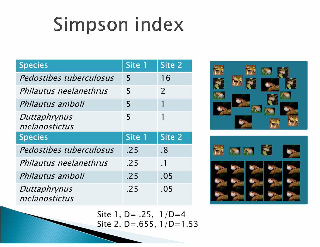
Species Site 1 Site 2
Pedostibes tuberculosus 5 16
Philautus neelanethrus 5 2
Philautus amboli 5 1
Duttaphrynusmelanostictus
5 1melanostictusSpecies Site 1 Site 2
Pedostibes tuberculosus .25 .8
Philautus neelanethrus .25 .1
Philautus amboli .25 .05
Duttaphrynusmelanostictus
.25 .05
Site 1, D= .25, 1/D=4Site 2, D=.655, 1/D=1.53

Claude Shannon and Warren Weaver in 1949◦ Developed a general model of communication and
information theory◦ Initially developed to separate noise from
information carrying signals◦ Subsequently, mathematician Norbert Wiener ◦ Subsequently, mathematician Norbert Wiener
contributed to the model as part of his work in developing cybernetic technology
Assumptions◦ All individuals are randomly sampled◦ Population is indefinitely large, or effectively infinite◦ All species in the community are represented

Equation◦ H’ = -S pi ln pi
pi = proportion of individuals found in the ith species Unknowable, estimated using ni / N Flawed estimation, need more sophisticated equation
(2.18 in Magurran)(2.18 in Magurran)
◦ Error Mostly from inadequate sampling Flawed estimate of pi is negligible in most instances
from this simple estimate

Species Site 1 Site 2
Pedostibes tuberculosus 5 16
Philautus neelanethrus 5 2
Philautus amboli 5 1
Duttaphrynusmelanostictus
5 1melanostictus
Species Site 1 Site 2
Pedostibes tuberculosus .25 .8
Philautus neelanethrus .25 .1
Philautus amboli .25 .05
Duttaphrynusmelanostictus
.25 .05
Site 1, H’= 1.39Site 2, H’=.71

Jaccard Index◦ Cj=j/(a+b-j), j is common to both a and b
community, a species in community a, b species in community in b,
Bray-Curtis dissimilarity Bray-Curtis dissimilarityS = (b+c)/(2a+b+c), ‘b’, ‘c’ are unique species ‘a’ is common to both

D=b+c/2a+b+cHIL HAR NAN NAG MAV HUR SHA
HAR 0.5NAN 0.5 0.57NAG 0.83 0.71 0.57MAV 0.75 0.66 0.67 0.67HUR 0.53 0.58 0.58 0.58 0.65SHA 0.68 0.74 0.62 0.62 0.68 0.68YEN 0.62 0.64 0.57 0.5 0.63 0.46 0.49
0.0 0.1 0.2 0.3 0.4Distances
HILKUNJI
HARIDRAVATHI
NANDIHOLE
NAGODIHOLE
MAVINAHOLE
HURLIHOLE
SHARAVATHI
YENNEHOLE

Thank you