國 立 交 通 大 學

資訊科學與工程研究所

碩 士 論 文

高 效 能 雲 端 儲 存 管 理 策 略 之 研 究

A Management Strategy of Replica Compression

for Hadoop

研 究 生：郭文俊

指導教授：蔡文能 教授

中 華 民 國 壹 佰 年 六 月

高 效 能 雲 端 儲 存 管理 策 略 之 研 究

A Management Strategy of Replica Compression for Hadoop

研 究 生：郭文俊 Student：Wen-Jun Guo

指導教授：蔡文能 Advisor：Wen-Nung Tsai

國 立 交 通 大 學

資 訊 科 學 與 工 程 研 究 所

碩 士 論 文

A Thesis

Submitted to Institute of Computer Science and Engineering

College of Computer Science

National Chiao Tung University

in partial Fulfillment of the Requirements

for the Degree of

Master

in

Computer Science

June 2011

Hsinchu, Taiwan, Republic of China

中華民國壹佰年六月

i

高效能雲端儲存管理策略之研究

學生：郭文俊 指導教授：蔡文能

國立交通大學資訊科學與工程研究所碩士班

摘要

我們提出一個雲端儲存副本管理策略，其利用少量儲存空間來保持資料可靠

性。為了儲存海量的資料，雲端儲存系統通常使用分散式檔案系統當作它的後端

儲存系統。自Google提出GFS(Google File System)後，Apache軟體基金會開發

了一個 Hadoop Distributed File System (HDFS)，其是一個提供Map/Reduce

框架計算的開放原始碼專案。為了改善系統可用性，檔案系統的架構採用資料複

製和機櫃感知的方法，當有節點掛掉時，至少仍可保持一份的資料副本在系統

中。然而，有兩個重要的問題需被考量，包含如何放置副本，以及如何減少因為

為了維持可用性所使用的資料複製而帶來的大量空間消耗。

在本篇論文中，我們提出一個副本管理策略來確保資料可用性以及減少空間

消耗。我們的方法根據自動地偵測網路拓墣，求出每個副本的適當位置。至於空

間消耗的問題，我們壓縮額外的副本在背景運作中，使得系統增加更多可用空

間。我們實作此策略在HDFS中，結果顯示此策略可以有效減少儲存空間，且不影

響系統效能。

ii

A Management Strategy of Replica Compression for

Hadoop

Student：Wen-Jun Guo Advisor：Wen-Nung Tsai

Institute of Computer Science and Information Engineering

National Chiao-Tung University

Abstract

We propose a replica management strategy for cloud computing, which

consumes minimum cost to keep data reliability for cloud storage. To store massive

data, cloud storage usually adopts distributed file system as its backend due to the

concern of scalability. With the GFS (Google File System) proposed by Google, the

Apache Software Foundation developed HDFS (Hadoop Distribute File System),

which is a primary storage system for computing with Map/Reduce framework. To

improve system availability, the file system architecture adopts data replication and

rack-awareness to preserve at least one copy when node crashes. However, two

important issues should be considered. These include how to place the replicas, and

how to reduce the large space consumption comes with duplicate replicas for the data

availability.

In this thesis, we present a replica management strategy to ensure the data

availability and to reduce the space consumption. Our method determines proper

places of each replica according to the network topology which is detected

automatically. As for the problem of space consumption, we compress the additional

copies of data in background. This makes the system increase more available space.

We implemented the strategy on HDFS. The results show that the proposed strategy

can effectively reduce the storage space, and will not affect system performance.

iii

誌謝

研究所兩年生活最要感謝的是我的老師－蔡文能教授，無論是課業還是研究

上，給了許多幫助以及寶貴的意見。在課業不順利時，盡其所能的幫助我在課業

上順利過關；在研究遇到瓶頸時，引導我如何去突破障礙，找到繼續研究的動力。

從老師身上，我學到了嚴謹的學術態度以及艱深的專業能力，這些將是我面臨未

來挑戰時用來突破困境的必備能力。

另外，還要感謝系計中的工作夥伴，在你們身上學到了高深的技術，以及認

真的處事態度，能與你們一起工作是我這生最快樂的時光。還有，感謝實驗室學

弟、同學熱心的建議，解決我許多研究的盲點。還有，感謝智瑋學長，在研究議

題以及學術論文寫作上提供專業的諮詢，才使得論文最後能順利完成。

最後，我要感謝我的家人，謝謝你們不求回報的關懷。在研究所的這段時間，

無論是精神上或是物質上，給了莫大的支持，使得我能無後顧之憂，順利完成我

的學業。在此，我由衷的感謝曾經幫過我的人，若沒有你們，也就沒有今天的我。

Table of Contents

1 Introduction 1

2 Background 3

2.1 The Goal of HDFS . . . . . . . . . . . . . . . . . . . . . . . . . . . . . . . . 3

2.2 HDFS Architecture . . . . . . . . . . . . . . . . . . . . . . . . . . . . . . . . 4

2.2.1 NameNode . . . . . . . . . . . . . . . . . . . . . . . . . . . . . . . . 4

2.2.2 DataNode . . . . . . . . . . . . . . . . . . . . . . . . . . . . . . . . . 5

2.2.3 HDFS Client . . . . . . . . . . . . . . . . . . . . . . . . . . . . . . . 6

2.3 Data Replication . . . . . . . . . . . . . . . . . . . . . . . . . . . . . . . . . . 7

2.4 Replica Placement . . . . . . . . . . . . . . . . . . . . . . . . . . . . . . . . . 7

3 Related Work 8

3.1 Hadoop’s Rack Awareness . . . . . . . . . . . . . . . . . . . . . . . . . . . . 8

3.2 System Parameter Based Replication Management . . . . . . . . . . . . . . . . 9

3.2.1 Model-Driven Replication . . . . . . . . . . . . . . . . . . . . . . . . 9

3.2.2 System Model . . . . . . . . . . . . . . . . . . . . . . . . . . . . . . . 10

3.2.3 Cost-Effective Dynamic Replication Management . . . . . . . . . . . . 11

3.3 Network RAID: DiskReduce . . . . . . . . . . . . . . . . . . . . . . . . . . . 13

3.3.1 Encoding Type . . . . . . . . . . . . . . . . . . . . . . . . . . . . . . 13

3.3.2 Background Encoding . . . . . . . . . . . . . . . . . . . . . . . . . . 14

3.4 Summary . . . . . . . . . . . . . . . . . . . . . . . . . . . . . . . . . . . . . 15

4 A Management Strategy of Replica Compression 17

4.1 Replica Placement . . . . . . . . . . . . . . . . . . . . . . . . . . . . . . . . . 17

4.1.1 Obtain location of DataNodes by using a topology detector . . . . . . . 19

4.1.2 Partition Network . . . . . . . . . . . . . . . . . . . . . . . . . . . . . 20

4.1.3 Locate Replicas . . . . . . . . . . . . . . . . . . . . . . . . . . . . . . 22

iv

4.2 Replica Management . . . . . . . . . . . . . . . . . . . . . . . . . . . . . . . 22

4.2.1 Background Compression . . . . . . . . . . . . . . . . . . . . . . . . 22

4.2.2 Real-Time Decompression . . . . . . . . . . . . . . . . . . . . . . . . 24

5 Implementation and Experimental Results 27

5.1 Implementation . . . . . . . . . . . . . . . . . . . . . . . . . . . . . . . . . . 27

5.1.1 Topology Detector . . . . . . . . . . . . . . . . . . . . . . . . . . . . 27

5.1.2 Compressor . . . . . . . . . . . . . . . . . . . . . . . . . . . . . . . . 29

5.2 Emulation Environment . . . . . . . . . . . . . . . . . . . . . . . . . . . . . . 30

5.3 Evaluation Criteria . . . . . . . . . . . . . . . . . . . . . . . . . . . . . . . . 31

5.3.1 Disk Space . . . . . . . . . . . . . . . . . . . . . . . . . . . . . . . . 31

5.3.2 Compression Time . . . . . . . . . . . . . . . . . . . . . . . . . . . . 32

5.3.3 Performance of Reading Data . . . . . . . . . . . . . . . . . . . . . . 32

5.4 Comparison . . . . . . . . . . . . . . . . . . . . . . . . . . . . . . . . . . . . 33

5.5 Issues . . . . . . . . . . . . . . . . . . . . . . . . . . . . . . . . . . . . . . . 34

5.5.1 Compressing Entire Replicas versus Partial Replicas . . . . . . . . . . 34

5.5.2 The Difference Between Rack-based and Network-based . . . . . . . . 35

5.5.3 Space Balancing . . . . . . . . . . . . . . . . . . . . . . . . . . . . . 35

6 Conclusion and Future Work 37

v

List of Tables

3.1 The System Parameters of Model-Driven . . . . . . . . . . . . . . . . . . . . . 10

3.2 The System Parameters of CDRM . . . . . . . . . . . . . . . . . . . . . . . . 12

4.1 The Parameters of the Probability for Data Reliability . . . . . . . . . . . . . . 18

5.1 The Specification of Hardware and Software . . . . . . . . . . . . . . . . . . . 30

vi

List of Figures

2.1 Hadoop Distributed File System Architecture . . . . . . . . . . . . . . . . . . 5

3.1 Hadoop Rack-Awareness . . . . . . . . . . . . . . . . . . . . . . . . . . . . . 9

3.2 The RAID5 and RAID6 Scheme in DiskReduce . . . . . . . . . . . . . . . . . 14

4.1 An Example to Explain the Risk of the Cluster in the Network . . . . . . . . . 18

4.2 Example: Partitioning Switch-level Network . . . . . . . . . . . . . . . . . . 20

4.3 Example: Partitioning Router-level Network . . . . . . . . . . . . . . . . . . . 21

4.4 Example: Client Sends a Request for Compressing the Files . . . . . . . . . . . 23

4.5 Example: Decompressing in Time and Replicating . . . . . . . . . . . . . . . . 25

4.6 Example: Full Scenario in an Environment of Network Layer 3 . . . . . . . . . 26

5.1 The Behavior of the Topology Detector in the L2 Network Environment . . . . 28

5.2 The Behavior of the Topology Detector in the L3 Network Environment . . . . 28

5.3 The Design of Compressor . . . . . . . . . . . . . . . . . . . . . . . . . . . . 29

5.4 The Comparison of Saved Space with Different Data . . . . . . . . . . . . . . 31

5.5 Comparing the Compression Time of System Logs and Web Pages . . . . . . . 32

5.6 Performance of Reading Data . . . . . . . . . . . . . . . . . . . . . . . . . . . 32

5.7 The Compression to MSRC and the Studies . . . . . . . . . . . . . . . . . . . 33

5.8 The Structure of the Well-planed Environment . . . . . . . . . . . . . . . . . . 35

5.9 The Case for Space Unbalancing . . . . . . . . . . . . . . . . . . . . . . . . . 36

vii

Chapter 1

Introduction

In recent years, cloud storage has become a popular research topic. With the rapid develop-

ment of the Internet, more and more storage requirements are moved to the Internet. Typically,

the storage that is accessed from the Internet is called the cloud storage. The ability of space

expansion in classic central storage is limited for single server architecture.

Storing data on the Internet that has many advantages. First, it is convenient for mobile

users. The users can access their data from anywhere via web and special supported client if

the network is available. Furthermore, The storage must guarantee to protect user privacy and

prevent data loss. The cloud storage vendors provide the features, which let users concentrate

on their work without worrying about data backup, protection and recovery. On the other hand,

the design on the architecture of cloud storage must be expandable. With the increase of data

storing requirement, a single central storage will encounter a bottleneck for storing a huge

amount of data. A single central storage will encounter the bottleneck for storing a huge amount

of data. The storage of the classic file system relies on the disk space of a single server. So,

the scalability depends the number of the slots on a centralized file server or RAID system.

Therefore, the classic file system is no longer adequate for large data storage.

In the general case, the cloud storage usually adopts a distributed file system as its back-end

because the distributed file system has many advantages can overcome the problems such as

fault tolerance, scalability and availability. The file system can store unlimited data if the design

is scalable to arbitrarily extend the space. So, The distributed file system is composed of nodes,

which is known as multiple servers. The distributed file system access files stored on nodes

via the network. Neither writing or reading, transmission with nodes that contains desirable

1

data needs to be done over network. Usually, a client which accesses the file may be able to

be treated as a node in the distribution system. The file system can aggregate the bandwidth of

the nodes. In theory the transmission capacity of a distributed system is the sum of the nodes

bandwidth. Besides, the good design of distributed system does not have the problem of a single

point of failure, which can be easily solved by the mechanism of tolerating partial nodes failure.

So, these features ensures the service that is always being is available during data transmission.

In 2003, Google proposed GFS (Google File System) [4], designed for scalability, availabil-

ity, and reliability. The design regards servers failed in the system as a normal behavior. The

distributed file system is composed of thousands of servers, so the probability of servers fail-

ure is higher. According to this, GFS replicates multiple copies of a block info different chunk

server for data reliability and availability. Based on the publication of Google’s MapReduce and

GFS , Apache foundation launches the Apache Hadoop project [13] as a version of open source

implementation. Apache Hadoop is a programming framework for MapReduce computing. It

uses the Hadoop Distributed File System (HDFS) [12] as its low-level file system. So, HDFS is

a special purpose of file system for Hadoop distributed programming . HDFS also implements

a few POSIX standards to provide the operation which is similar to the classic file system, but

its performance is lower because it is designed for MapReduce programming. Both of GFS and

HDFS are designed for data-intensive computing purpose. Because of HDFS is open source and

a clone of GFS. Neither replicas placement or replica management the design is very similar.

Thus, we choose HDFS as our research platform and implement on it for system evaluation.

In order to meet the data availability and reliability, the architecture of HDFS adopts data

replication, which keeps at least one copy of a block when some nodes have no response. How-

ever, the replicas placement, which is a key problem, ensures the replicas of the data are not in

the critical or closed node while network cable is broken or machines failure. Besides, although

the storage pool can be arbitrarily and dynamically extended space, which stored data for fault

tolerance, but both of the cost of the space and space utilization are disproportionate.

In this thesis, we aim to save disk space and effectively divide up critical groups of a net-

work for placing replicas. The proposed method only costs small space to provide the feature

of fault tolerance, and it can automatically determine better replicas location in any network

environments. Thus, the system administrator does not require to manually maintain a list for

server location.

2

Chapter 2

Background

Since Google has published Google File System (GFS) and MapReduce papers, Apache

launched a project named Apache Hadoop, which is used for data-intensive computing. Hadoop’s

storage system is called Hadoop Distributed File System (HDFS), which is designed for storing

large amount of data. In this requirement, many challenges in the distributed environment that

should be overcame. So the following sections will introduce the goal, design and how to meet

the issues of HDFS.

2.1 The Goal of HDFS

The goal of HDFS is to compute large amounts of data. That is very different than a

classic file system such as Ext2, Ext3 and UFS. The major programming on HDFS is called

Map/Reduce programming. The applications are written by using Map/Reduce framework that

can employ the powerful capacity to process datasets (e.g., system log analysis, machine learn-

ing, data mining). Thus, the features for the computing will be described as the following three

points.

Tolerance to Server Failure

In the past, a single server has a problem of single point of failure (SPOF). When a central-

ized server fails, the whole system does not service anymore. So as to overcome the problem,

HDFS adopts distributed architecture and data replication. When a node is non-functional, one

3

of nodes will take over and recover the data. The action of detection and recover action is auto

by system-self. So the system has a high degree of capacity of self repair.

Large Data Storing

The capacity of a single server which stores large data is limited because the expanded ca-

pacity of disks is limited. So, HDFS cascades nodes space via network, and effectively manages

the index which maps the blocks of file to a node. Therefore, HDFS has enough ability to handle

the processing for large amount of data.

Portability and Scalability

Because of storing data in network nodes, the design considers the software that may run on

different operating system and hardware architecture. For the portability, HDFS is written by

Java such that easily migrate to various systems.

2.2 HDFS Architecture

The HDFS is composed of two types of nodes: NameNode and DataNode. Usually, The

number of DataNodes is greater than the number of NameNodes. The section will explain the

role and responsible job of the nodes.

2.2.1 NameNode

The NameNode maintains a file system namespace to record a structure of file and directo-

ries. The structure is tree hierarchy, which means it is similar to a classic file system composed

of files and directories. HDFS also uses inode to represent some file attributes, such as permis-

sion, modification and access times. A file on HDFS is split into multiple block to store into

DataNods. Each block size is 64MB by default. The unit of data replication is a block instead of

a file. In addition to namespace, The NameNode is also responsible to maintain a table, which

maps the blocks of files to DataNodes. The entire namespace and block map are stored in

4

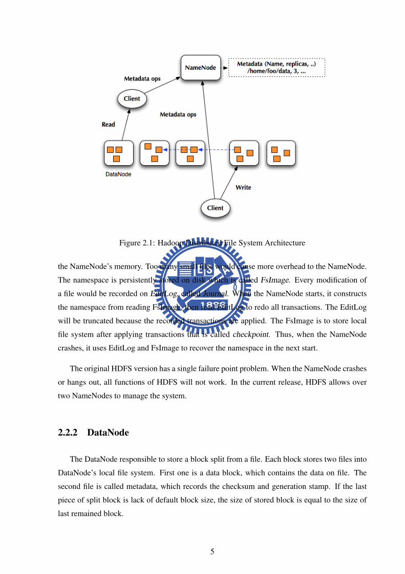
Figure 2.1: Hadoop Distributed File System Architecture

the NameNode’s memory. Too many small files would cause more overhead to the NameNode.

The namespace is persistently stored on disk which is called FsImage. Every modification of

a file would be recorded on EditLog, called Journal. When the NameNode starts, it constructs

the namespace from reading FsImage, then read EditLog to redo all transactions. The EditLog

will be truncated because the recorded transactions are applied. The FsImage is to store local

file system after applying transactions that is called checkpoint. Thus, when the NameNode

crashes, it uses EditLog and FsImage to recover the namespace in the next start.

The original HDFS version has a single failure point problem. When the NameNode crashes

or hangs out, all functions of HDFS will not work. In the current release, HDFS allows over

two NameNodes to manage the system.

2.2.2 DataNode

The DataNode responsible to store a block split from a file. Each block stores two files into

DataNode’s local file system. First one is a data block, which contains the data on file. The

second file is called metadata, which records the checksum and generation stamp. If the last

piece of split block is lack of default block size, the size of stored block is equal to the size of

last remained block.

5

2.2.3 HDFS Client

HDFS provides a series operations similar to the classic file system (e.g., read, write, delete).

A file or directory is accessed according to the path in the namespace. The HDFS is transparent

to the client. That means it does not know how HDFS works and where the block are stored.

They only concentrate on run their job. If an application wants to use HDFS, they must through

API provided by HDFS. HDFS , which exposes interfaces (HDFS API) for any applications,

are easy to use operations of HDFS. For instance, A Map/Reduce program can use the API to

schedule tasks for improving performance.

Reading

When a client sends a request of reading files, first it will communicate with the NameN-

ode for which blocks constitute the file and where the replicas of the blocks. By default, one

communication will ask NameNode for ten blocks information. Yet, the replicas of the block

are sorted by NameNode according to the location of client and replicas. The client refers the

replica location information, then send a block reading request to the DataNode. Now begin to

transfer the desired block.

Writing

Writing procedure is similar to reading procedure. When a client sends a request of writing,

it also asks the NameNode for available DataNodes first. The NameNode replies the DataNodes

information to client. Then, the client writes a block of data to first DataNode which is from

the information. After writing a first block, the block will be replicated to the other DataNodes

by received DataNodes, until the current number of the replicas equals to replica factor of file.

This process is called Pipeline Writing. Therefore, although the blocks have many copies, the

client only write one time. Neither reading or writing, when the desired DataNode has error,

the client will choose another available DataNodes to continue the job. Each failure in reading

or writing the pipeline will be re-organized as new pipeline.

6

2.3 Data Replication

Most distributed file systems usually split a file into multiple blocks to store. Either reading

or writing is through multiple storage source to increase system performance like RAID5. Data

replication is one of methods which ensures data always has at least one copy available. The

function is quite useful and straightforward to implement. It can make data protection in block-

level. Block-level protection has many benefits. One is when the partial data are corrupt or

unavailable, only missed blocks must be rebuilt or re-sent.

Typically, more than two copies are put on different storage that can improve data reliabil-

ity. When a client reads blocks of data from multiple sources, the performance is better than

accessing from only one source. Thus, what is the number of replicas is better in HDFS that is

a key problem. If replica factor is set too high, that may increase performance and availability

but actually free space is reduced and increase the cost of storage. Moreover, it may exhaust

the network bandwidth so that performance is not as expected result. The optimal situation is

to use minimum replica to satisfy requirement of performance and availability.

2.4 Replica Placement

The current HDFS replica placement strategy follows a simple rule. That attempts to im-

prove data reliability and access performance. So, Apache released version of Hadoop uses

three copies of a block as a default replica factor.

The first copy is put on local DataNode. That means the block is written on local disk

because the client is usually regarded as DataNode. The speed of local disk access is faster

than the speed network transmission. After first copy written completely, it will be replicated

to the other DataNodes by using pipeline. The second copy will be chosen to locate at the far

distance to store. The distance factor is compared to location of DataNodes which has first one.

This idea is a concerns for data reliability because the data which are put on two nodes with

farthest distance is the safest. In contrast, the two nearest is unsafe because both of them are

able connected to the same network device or power supply. If the device crashes or the power

is cut off, the data would be loss. The third copy is located on a different DataNode at first the

rack but different host than first one. Because of second copy has ensured data reliability, the

location concern of the last copy is main for performance. The nearest copies can improve the

read/write performance.

7

Chapter 3

Related Work

This chapter will introduce the work whose goal is relative to our work. Hadoop’s pro-

posed method will present at the first section, and then present the proposal that deals with

data reliability, and the last section will show the method which solves the problem of space

consumption.

3.1 Hadoop’s Rack Awareness

Hadoop uses rack-awareness [14] method to increase system availability and performance.

This idea was first proposed on the website of the project, and then implemented into Hadoop

software as a basic function eventually.

The feature assumes HDFS must run on the environment constructed as tree hierarchical

network topology. Specifically, the network devices, server and rack must be structured as

a Hadoop cluster beforehand rather than arbitrarily construct that. So, one rack only has one

switch and devices link with the switch in the rack. The layout forms a tree logically hierarchical

structure. Each DataNodes has an identical default ID in rack-awareness method. To use the

method,the DataNodes must be configured with an unique ID. The ID consists of data center and

rack number which implies the location of the DataNode. When a DataNode requests to join

a cluster, it sends its ID to the NameNode. The NameNode confirms the node which wants to

join the cluster whether exists in the map, and then add entry or update the map. If a DataNode

does not provide its ID, it uses the default ID and belongs to default group in the map. After all

DataNodes have joined the cluster successfully, the NameNode is responsible to maintain the

8

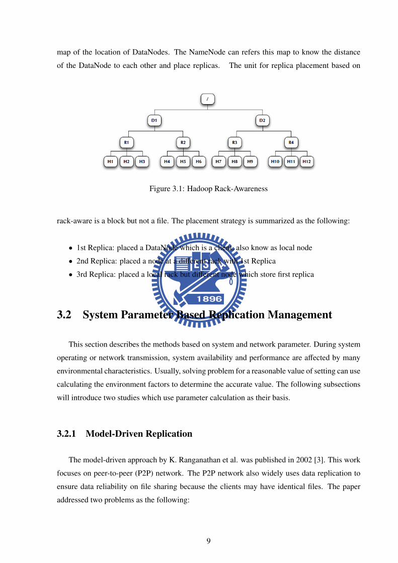
map of the location of DataNodes. The NameNode can refers this map to know the distance

of the DataNode to each other and place replicas. The unit for replica placement based on

Figure 3.1: Hadoop Rack-Awareness

rack-aware is a block but not a file. The placement strategy is summarized as the following:

• 1st Replica: placed a DataNode which is a client, also know as local node

• 2nd Replica: placed a node at a different rack with 1st Replica

• 3rd Replica: placed a local rack but different node which store first replica

3.2 System Parameter Based Replication Management

This section describes the methods based on system and network parameter. During system

operating or network transmission, system availability and performance are affected by many

environmental characteristics. Usually, solving problem for a reasonable value of setting can use

calculating the environment factors to determine the accurate value. The following subsections

will introduce two studies which use parameter calculation as their basis.

3.2.1 Model-Driven Replication

The model-driven approach by K. Ranganathan et al. was published in 2002 [3]. This work

focuses on peer-to-peer (P2P) network. The P2P network also widely uses data replication to

ensure data reliability on file sharing because the clients may have identical files. The paper

addressed two problems as the following:

9

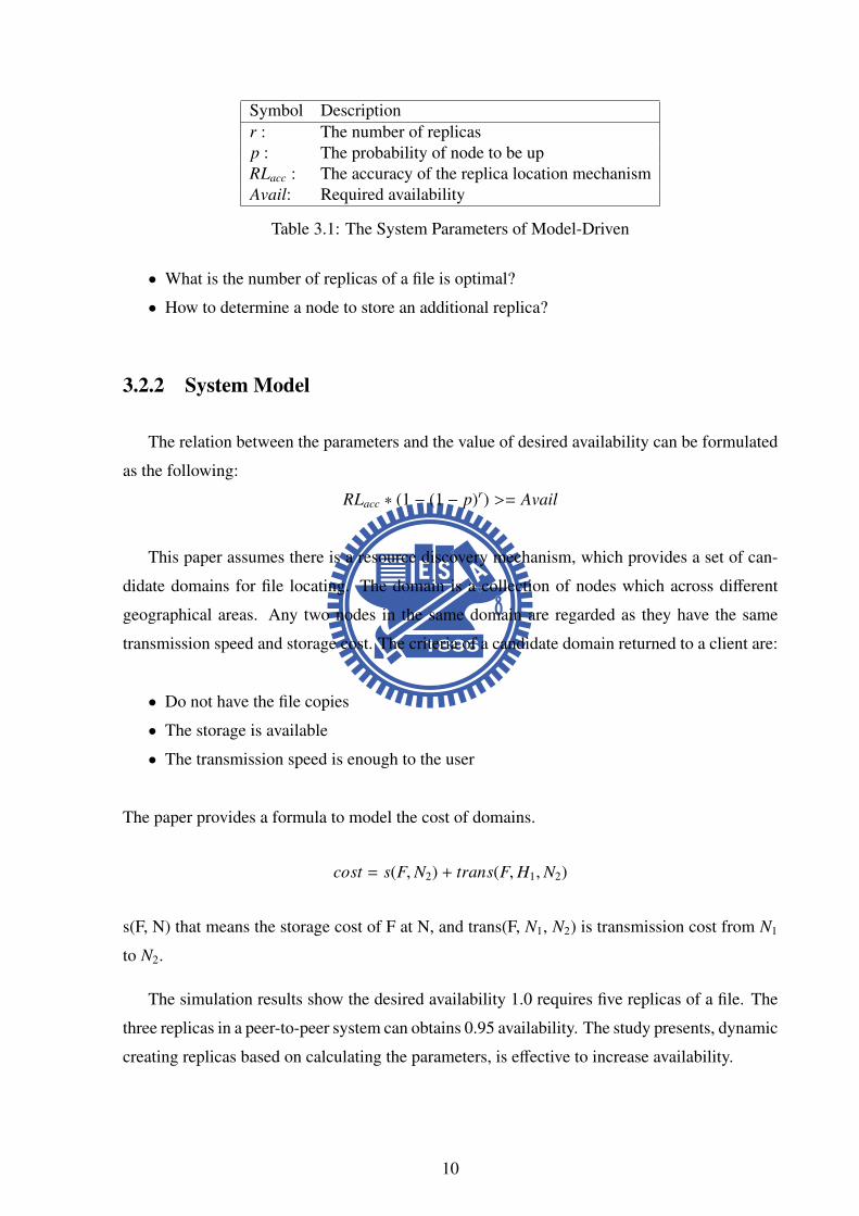
Symbol Descriptionr : The number of replicasp : The probability of node to be upRLacc : The accuracy of the replica location mechanismAvail: Required availability

Table 3.1: The System Parameters of Model-Driven

• What is the number of replicas of a file is optimal?

• How to determine a node to store an additional replica?

3.2.2 System Model

The relation between the parameters and the value of desired availability can be formulated

as the following:

RLacc ∗ (1 − (1 − p)r) >= Avail

This paper assumes there is a resource discovery mechanism, which provides a set of can-

didate domains for file locating. The domain is a collection of nodes which across different

geographical areas. Any two nodes in the same domain are regarded as they have the same

transmission speed and storage cost. The criteria of a candidate domain returned to a client are:

• Do not have the file copies

• The storage is available

• The transmission speed is enough to the user

The paper provides a formula to model the cost of domains.

cost = s(F,N2) + trans(F,H1,N2)

s(F, N) that means the storage cost of F at N, and trans(F, N1, N2) is transmission cost from N1

to N2.

The simulation results show the desired availability 1.0 requires five replicas of a file. The

three replicas in a peer-to-peer system can obtains 0.95 availability. The study presents, dynamic

creating replicas based on calculating the parameters, is effective to increase availability.

10

3.2.3 Cost-Effective Dynamic Replication Management

Cost-Effective Dynamic Replication Management by Q. Wei et al. was published in 2010

[9]. The paper addressed two problems in the replicas management:

• How many replicas should be kept to satisfy high availability requirement?

• How to place replicas to maximize system performance and balance loading?

For solving these problems, the authors formulate the parameters from two aspects, which are

availability and block probability. Using the formulations can derive the best value such as the

number of replica and replica location.

System Model

The distributed file system can be separated several different components to model in order

to derive the accurate result. The system consists of N independent nodes, which store M

different blocks. b1,b2,...bM denotes blocks. The Bi = bi1, bi2, ...biM is denoted the set of

the node S i stores M different blocks. b j = (pi, s j, r j, τa) denotes a set of attribute of block

b j. They denotes popularity, size, replica number and access latency of a block, respectively.

S j = (λ j, τ, f j, bw j) denote a set of attributes of node S i, which are request arrive rate, average

service time, failure probability, and network bandwidth respectively.

The paper provides a formulation to decide how large the network bandwidth is sufficient to

the performance requirement of the node.

bwi ≥ci∑

j=1

s j

τ j

It indicates the bandwidth of the each session is calculated by s j/τ j. So the bandwidth re-

quirement of data node S j is greater equal than the bandwidth of all sessions the node serves.

Availability

The probability of node availability is denoted as P(NA). P(N̄A) is the opposite of meaning.

The relation between both of them is P(NA) = 1 − P(N̄A). P(BAi) denotes the probability of

11

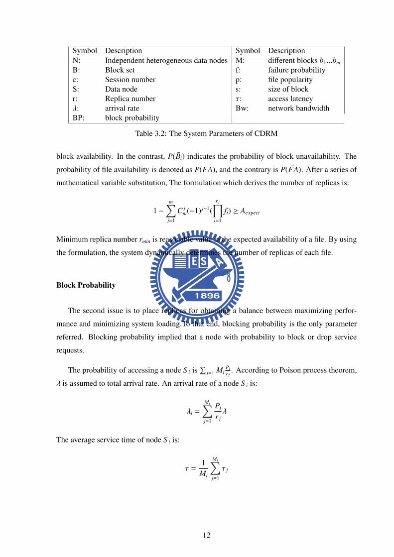
Symbol Description Symbol DescriptionN: Independent heterogeneous data nodes M: different blocks b1...bm

B: Block set f: failure probabilityc: Session number p: file popularityS: Data node s: size of blockr: Replica number τ: access latencyλ: arrival rate Bw: network bandwidthBP: block probability

Table 3.2: The System Parameters of CDRM

block availability. In the contrast, P(B̄i) indicates the probability of block unavailability. The

probability of file availability is denoted as P(FA), and the contrary is P(F̄A). After a series of

mathematical variable substitution, The formulation which derives the number of replicas is:

1 −m∑

j=1

C jm(−1) j+1(

r j∏i=1

fi) ≥ Aexpect

Minimum replica number rmin is reasonable value in the expected availability of a file. By using

the formulation, the system dynamically determines the number of replicas of each file.

Block Probability

The second issue is to place replicas for obtaining a balance between maximizing perfor-

mance and minimizing system loading.To that end, blocking probability is the only parameter

referred. Blocking probability implied that a node with probability to block or drop service

requests.

The probability of accessing a node S i is∑

j=1 MiPir j

. According to Poison process theorem,

λ is assumed to total arrival rate. An arrival rate of a node S i is:

λi =

Mi∑j=1

Pi

r jλ

The average service time of node S i is:

τ =1

Mi

Mi∑j=1

τ j

12

Finally, The blocking probability of node is S i modelled as M/G/ci system

BPi =(λiτ j)ci

ci!

ci∑k=0

(λiτ j)k

k!

−1

A node with low blocking probability has high priority to be chosen as a replica location due to

the node has a lower loading than the others. The NameNode uses B+ tree to store BP (Block

Probability) for accelerating search speed. The value of blocking probability is a key and node

ID is a value are stored in the structure. Thus, the NameNode can quickly find the node with low

BP value in the record of the thousands of nodes. The blocking probability is a useful criterion

for replica placement and load balancing.

The strategy is implemented to Hadoop for emulation. The experimental results show, the

system has greater than 0.9 availability is required to keep about four replicas. Moreover, the

difference of the system utilization is very smaller than the unmodified version of Hadoop.

That means, the study efficiently balances the nodes loading, and uses less replicas to keep

availability than the the previous studies.

3.3 Network RAID: DiskReduce

DiskReduce by B.Fan et al. was published in 2010 [8]. In the paper, the aim is to reduce disk

space based on Redundant Array of Independent Disks (RAID) data storage scheme. DiskRe-

duce is a kind of network RAID. Due to the performance concern, DiskReduce executes the

data encoding in the background. The redundant blocks are not deleted during an encoding

phase until the encoding phase completes. Thus, the available space in the system will grow

after encoding process.

3.3.1 Encoding Type

The study proposes two prototypes: RAID5 and RAID6. Each scheme has different capacity

of reducing the space. By default, three copies are used in the system.

13

Figure 3.2: The RAID5 and RAID6 Scheme in DiskReduce

RAID5

This scheme maintains a fully mirror version and a RAID5 parity set. The parity set is

required to recover the data if all mirrored copies of the block are not available. In a nutshell,

one of the copies of the block is encoded as a parity set. The reduced storage overhead is 1+1/N,

where N indicates how many blocks are calculated as a parity set.

RAID6

The difference between RAID5 and RAID6 is the number of full backups of blocks. The

feature of RAID is encoding additional copies instead of the full backup. The scheme can also

tolerate double copies failed like RAID5 scheme. It maintains one copy and double parity set.

The storage overhead only remains 2/N, where N denotes how many blocks are calculated as

a parity set. Both of them are implemented on userspace of HDFS. The results show, RAID5

scheme can reduce 40% overhead in storage capacity, and RAID6 can reduce 70% overhead

because RAID6 have two parity set instead of two full backs.

3.3.2 Background Encoding

HDFS replicates the block in the background. The concern of running in the background

is to facilitate the overhead of implementation. The process spends little time during encoding.

In general, increasing the number of copies can improves performance. The paper describes

14

three issues to discuss because the copies in DiskReduce implementation are less than or orig-

inal HDFS. The below will shows three reason reduce copies number might cause low perfor-

mance. First reason is duplicated tasks. During Map/Reduce processing, once the computing

node crashes or long time to response, the job which the node have that will be taken by an-

other node. Above is called Backup task. The attention is, the choice is prefer the node which

have local copies which same the original node. Otherwise, that will consume much network

bandwidth because the backup task will occupy part of the bandwidth. Finally the computing

performance will decrease more than no backup task mechanism. Second reason is disk band-

width. According this paper, popular file usually is small size data. If decreasing the number of

copies, a part of nodes which have the popular file will become a bottleneck. The GFS design

allows a file have many copies that over three copies if necessary. Third reason is load balanc-

ing. The data are randomly distributed within the nodes, but it may not be evenly distributed.

The result causes execute Map/Reduce with choosing node has local copies preferably is load-

ing unbalance. If have many copies, the job tracker can efficiently assign tasks such that nodes

loading will be balanced.

The method is implemented on Hadoop. The experimental result shows, it reduces the

overhead of space from 200% 125% to by using RAID6 scheme. Even if only one copy of

blocks serves the requests, the performance gets little penalty. Hence the study is very practical

and useful to reduce the high overhead of space.

3.4 Summary

The studies solve the problem of availability, performance and space respectively on a clus-

ter. Implementing on HDFS is mainstream because HDFS is a very popular platform for build-

ing a cloud storage. The researches have the common goal is how to minimize cost to maximize

performance under guaranteeing the availability situation.

Hadoop Rack-Awareness

Although the study solves the problems, there are some issues are not being considered or

bring new issue. Through well-planing DataNodes location, replicas will be placed into appro-

priate node. If the network structure is built with the racks layout, the system has the ability

to handle power outage or network accidents. However, the network environment and servers

15

should match the assumption constructed as tree hierarchical network topology. Furthermore,

manager manually maintains a list to record the location of DataNodes in racks. Unfortunately,

many environments are non-structural, which implies general network environments with lim-

ited cost have no well-planed physical network environment. To recode the location of servers,

maintaining thousands of servers is trouble for system administrators.

System Parameter based

The studies of system parameter based can accurately measure various factors in a system by

using network and system characteristics. The result shows it requires many replicas to improve

performance and availability. In contrast, high replica number comes with several times space

overhead is a serious problem. Although raising replica factor of popular file or lowering replica

factor of unpopular file is dynamic. On average the number of replicas is greater than four. That

is, only less than a quarter of the real space can be used. Furthermore, the method does not

consider the location of the node that cannot guarantee availability. Once all replicas of a block

of a file are placed in identical node, the file will lose when the node crashes. Thus, placing

replicas according to the nodes location is better than increasing replica factor for availability.

DiskReduce

DiskReduce applies the concept of RAID in HDFS. By using data encoding that effectively

reduces the space overhead spending additional space to store replicas for data protection. Spe-

cially, performance is not reduced too much. However, DiskReduce has the lack of flexibility

which cannot let a user specify which file has to be encoded. On the other hand, decoding the

encoded file is difficult because the system cannot control which files to be grouped for RAID

encoding.

According to the drawbacks, next chapter we present our method, whose one of functions

enhances Hadoop’s rack-awareness, and the function of reducing disk space is more flexible

than DiskReduce.

16

Chapter 4

A Management Strategy of Replica

Compression

This chapter describes the detailed management strategy of our scheme named MSRC

(Management Strategy of Replica Compression). The strategy is divided into two parts, replica

placement and replica management respectively. The section of replica placement describes

how to choose a location for replicas is appropriate, and the section of replicas management

presents the method to increase the free space of the storage.

4.1 Replica Placement

The placement idea is mainly inspired by Hadoop’s rackaware, but based on the network

topology instead of the location of physical racks. Replica location is more crucial than in-

creasing the number of replicas to protect data. However, any network can be seen as multiple

sub-networks groups. The links between the core device and a sub-network group is a criti-

cal path. If any critical path breaks, at least one host will disappear in the network and some

replicas will be lost for the distributed system.

For instance, Figure 4.1 is a cluster whose servers are distributed in the network. Logically,

the network is considered as three sub-network groups. To keep data reliability, how to avoid

placing the replicas of a block in the identical group is a major issue. If the placement is non-

17

Figure 4.1: An Example to Explain the Risk of the Cluster in the Network

location-based, the relation of a network and replica can be modelled as the following formula.

B = (1/g)r−1 ∗ F ∗ N

The formula shows the number of replicas cannot guarantee data reliability because randomly

Symbol DescriptionB the number of blocks replicas are in the same groupr replica factorg the number of partitioned groupsF the number of filesN one file consist of N blocks

Table 4.1: The Parameters of the Probability for Data Reliability

placing replicas causes all replicas of some file is in an identical sub-network. The system can-

not serve users with high availability. So, our method is network-location-based that attempts

to locate DataNodes in order to avoid the situation happening. It consists of three order phases.

• Obtain location of the DataNodes by using a topology detector

• Partition network

• Locate replica

18

4.1.1 Obtain location of DataNodes by using a topology detector

The topology detector provides administrators with two options of network type, switch

level (Layer 2 Network) and network level (Layer 3 Network) based on OSI (Open System

Interconnection) model. Because different network types use various bases to be logically sep-

arated into sub-network groups, the administrator must pre-configure the used network type

before using the detector.

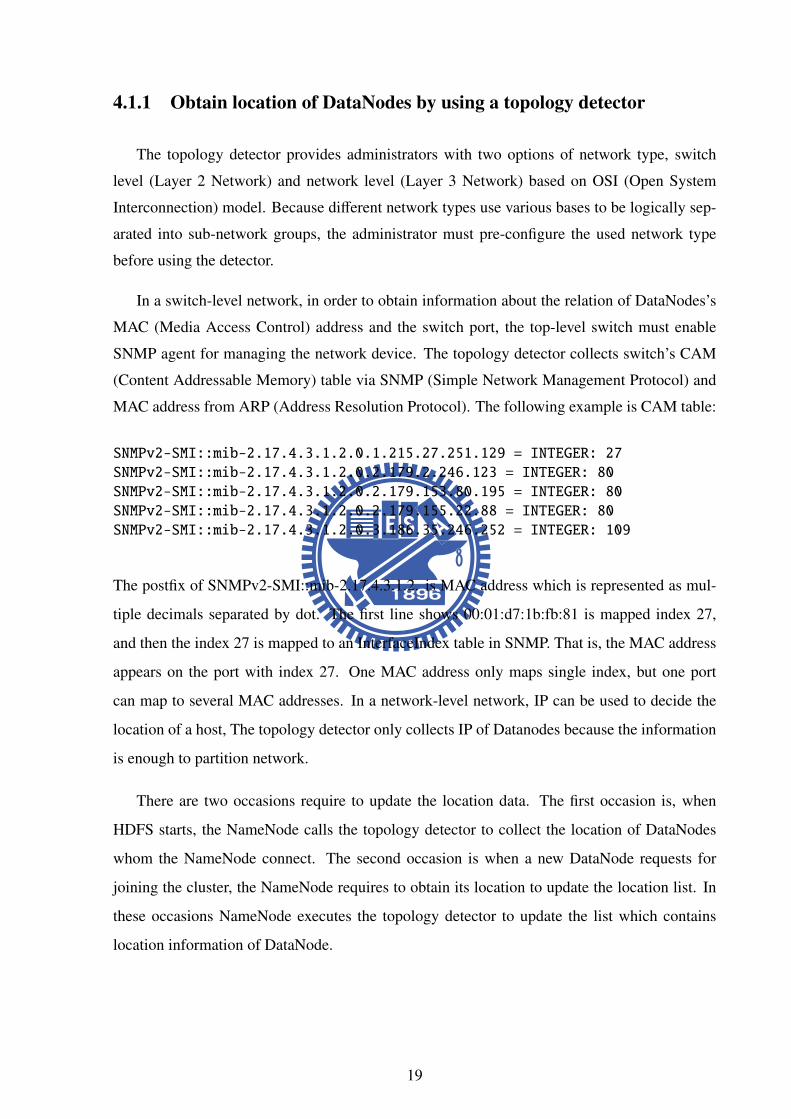
In a switch-level network, in order to obtain information about the relation of DataNodes’s

MAC (Media Access Control) address and the switch port, the top-level switch must enable

SNMP agent for managing the network device. The topology detector collects switch’s CAM

(Content Addressable Memory) table via SNMP (Simple Network Management Protocol) and

MAC address from ARP (Address Resolution Protocol). The following example is CAM table:

SNMPv2-SMI::mib-2.17.4.3.1.2.0.1.215.27.251.129 = INTEGER: 27SNMPv2-SMI::mib-2.17.4.3.1.2.0.2.179.2.246.123 = INTEGER: 80SNMPv2-SMI::mib-2.17.4.3.1.2.0.2.179.153.80.195 = INTEGER: 80SNMPv2-SMI::mib-2.17.4.3.1.2.0.2.179.155.22.88 = INTEGER: 80SNMPv2-SMI::mib-2.17.4.3.1.2.0.3.186.35.246.252 = INTEGER: 109

The postfix of SNMPv2-SMI::mib-2.17.4.3.1.2. is MAC address which is represented as mul-

tiple decimals separated by dot. The first line shows 00:01:d7:1b:fb:81 is mapped index 27,

and then the index 27 is mapped to an InterfaceIndex table in SNMP. That is, the MAC address

appears on the port with index 27. One MAC address only maps single index, but one port

can map to several MAC addresses. In a network-level network, IP can be used to decide the

location of a host, The topology detector only collects IP of Datanodes because the information

is enough to partition network.

There are two occasions require to update the location data. The first occasion is, when

HDFS starts, the NameNode calls the topology detector to collect the location of DataNodes

whom the NameNode connect. The second occasion is when a new DataNode requests for

joining the cluster, the NameNode requires to obtain its location to update the location list. In

these occasions NameNode executes the topology detector to update the list which contains

location information of DataNode.

19

4.1.2 Partition Network

This phase introduces how to group adjacent DataNodes. On the physical network topology,

the adjacent DataNodes are linked to the identical network device. If the port which the DataN-

odes linked is failed, these DataNodes will break simultaneously. So, the objective of the phase

is to partition the network into multiple sub-network groups as a unit for the replica placement.

When the data have been collected by the NameNode at the previous phase, the NameNode

tags each DataNode with a group ID for indenting which group the DataNode belongs. If

the DataNodes have the same group ID, it implies that the DataNodes belong to the identical

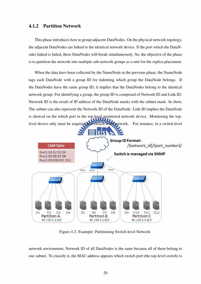
network group. For identifying a group, the group ID is composed of Network ID and Link ID.

Network ID is the result of IP address of the DataNode masks with the subnet mask. In short,

The subnet can alto represent the Network ID of the DataNode. Link ID implies the DataNode

is showed on the which port in the top-level monitored network device. Monitoring the top-

level device only must be required in a switch-level network. For instance, in a switch-level

Figure 4.2: Example: Partitioning Switch-level Network

network environment, Network ID of all DataNodes is the same because all of them belong to

one subnet. To classify it, the MAC address appears which switch port (the top-level switch) is

20

the basis. The DataNodes in the different ports that implies the DataNodes belongs to various

network groups. In a router-level network environment, Network ID is calculated by IP of the

DataNode and default subnet netmask 255.255.255.0 with AND operation. The Link ID of all

of DataNodes is the same because there is no the monitored network device. Thus, Link ID is a

default value (zero). Obviously, Partitioning a switch-level network only uses MAC address for

DataNodes classification, and a router-level network only uses IP to partition.

As shown in Figure 4.2, only a top-level network device (switch1) is monitored via SNMP

by the topology detector. In this case, the NameNode sends an SNMP request to the device for

obtaining CAM table, D1, D2, D3 and D4 appeared on the first switch port, and are labelled as

an identical group ID "/10.1.1.0/1". D5, D6, D7 and D8 appeared on the second switch port,

and labelled as an identical group ID "/10.1.1.0/2", and so on. Finally, the network is to be

partitioned into three network groups logically by three group IDs. As Figure4.3 shows, the

Figure 4.3: Example: Partitioning Router-level Network

network is partitioned by DataNodes’ IP and netmask 255.255.255.0. Servers within a subnet

are labelled as a group ID. There are four sub-networks, where the DataNodes locate are labelled

as "/10.1.1.0/0", "/10.1.2.0/0", "/192.168.1.0/0" and "/192.168.2.0/0". Notice that Link ID value

is zero. In short, the grouping basis is according to the links of the router in this example.

21

4.1.3 Locate Replicas

After partitioning the network, the NameNode decides how to place the replicas of a block

into multiple DataNodes. Due to data reliability, three copies are used as a default replica

factor to avoid data loss when DataNodes crash or no response. Hadoop’s placement policy is

straightforward, so the rule of MSRC follows original rule of HDFS.

The first block is placed on local storage due to file locality. Typically, the speed of local

transmission is faster than the speed of network transmission. The second copy of the block is

placed on a DataNode in different network groups with respect to the first copy. The third copy

of the block is placed on local network group but different from the node which has the first

copy. The difference between Hadoop’s Rack-Awareness and MSRC is the unit of DataNodes

group is changed from rack to network group.

4.2 Replica Management

Whereas block replication can protect data for reliability, it also raises a problem of wasting

space. To solve the problem, MSRC uses the compression method to decrease the overhead of

the space. This section will introduce what the occasion to compress and decompress additional

replicas, and give examples to explain the detailed flow.

4.2.1 Background Compression

In order to increase more free space, the redundant replicas on DataNodes must be com-

pressed. Hadoop adopts a block of a file with three copies, which are placed into different

DataNodes to prevent data loss when DataNode is broken. The number of replicas that depends

on configuration setting. The user can increase the value for high data protection. This is the

simplest and effective way to ensure the data are always available.

To ease the overhead, MSRC provides a role named Compressor. The Compressor provide

client specifies the files which match some file attributes to be compressed, such as file/directory

name and access time. The reason of providing access time to be specified is if the files have

22

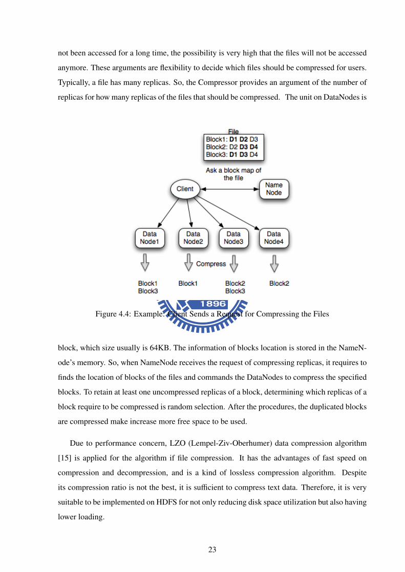
not been accessed for a long time, the possibility is very high that the files will not be accessed

anymore. These arguments are flexibility to decide which files should be compressed for users.

Typically, a file has many replicas. So, the Compressor provides an argument of the number of

replicas for how many replicas of the files that should be compressed. The unit on DataNodes is

Figure 4.4: Example: Client Sends a Request for Compressing the Files

block, which size usually is 64KB. The information of blocks location is stored in the NameN-

ode’s memory. So, when NameNode receives the request of compressing replicas, it requires to

finds the location of blocks of the files and commands the DataNodes to compress the specified

blocks. To retain at least one uncompressed replicas of a block, determining which replicas of a

block require to be compressed is random selection. After the procedures, the duplicated blocks

are compressed make increase more free space to be used.

Due to performance concern, LZO (Lempel-Ziv-Oberhumer) data compression algorithm

[15] is applied for the algorithm if file compression. It has the advantages of fast speed on

compression and decompression, and is a kind of lossless compression algorithm. Despite

its compression ratio is not the best, it is sufficient to compress text data. Therefore, it is very

suitable to be implemented on HDFS for not only reducing disk space utilization but also having

lower loading.

23

4.2.2 Real-Time Decompression

After completing replica compression, the available replicas of a block for access remain a

limited number of the replicas. The response from the NameNode to the client is changed. The

NameNode only replies the location of the uncompressed replicas to the client. Only in the two

conditions, the compressed data should be transmitted to the client for access:

• The DataNode is failed

If the DataNodes which contain the replicas of the block is unavailable, there is no un-

compressed block can service the request for the client. So, the NameNode attempts to

return the location of the compressed replicas to the client, and then the client sends a

request to the DataNode which contains the compressed replica for block access. At this

time, DataNode transmits compressed data to the client. The client decompresses the

compressed block in time and reads the content. Thus, the client will not miss any data

even if DataNodes cannot service the request of accessing block.

• Supplying replica

In the previous condition, DataNode crashing that cause some replicas missing. The

number of current replica is lower than a replica factor of the setting. So, in this situation

MSRC will automatically start replicating block until the number of replicas is equal to

the replica factor in the setting. If no uncompressed block can be sent to another host for

supplying replica, there are only compressed block can serve it. The DataNode transmits

the compressed block to another DataNode, and then the received DataNode uncompress

the block and stores again. The replication procedure still requires to meet the placement

strategy of MSRC.

After introducing MSRC, Figure 4.6 is a full example of MSRC to completely explain the

flow. The environment is a kind of router-level network, which are composed of two routers and

four switches. Each router connects two switches within an absolute subnet. and each switch

connects fours DataNodes. The client has two files, which are split into three blocks, called

block A, B and C respectively. The default replica factor is three copies so the used space of the

cluster is three times as big as the total size of the files.

24

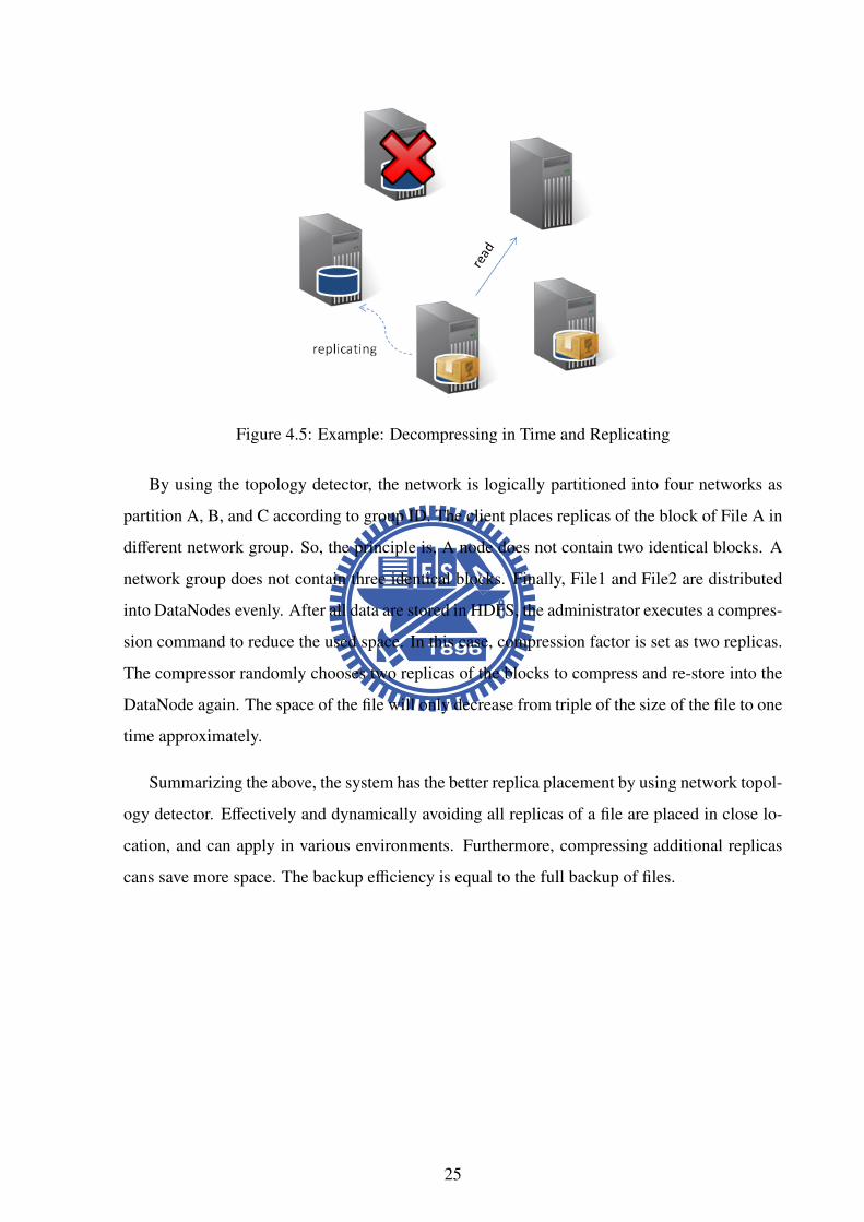
Figure 4.5: Example: Decompressing in Time and Replicating

By using the topology detector, the network is logically partitioned into four networks as

partition A, B, and C according to group ID. The client places replicas of the block of File A in

different network group. So, the principle is, A node does not contain two identical blocks. A

network group does not contain three identical blocks. Finally, File1 and File2 are distributed

into DataNodes evenly. After all data are stored in HDFS, the administrator executes a compres-

sion command to reduce the used space. In this case, compression factor is set as two replicas.

The compressor randomly chooses two replicas of the blocks to compress and re-store into the

DataNode again. The space of the file will only decrease from triple of the size of the file to one

time approximately.

Summarizing the above, the system has the better replica placement by using network topol-

ogy detector. Effectively and dynamically avoiding all replicas of a file are placed in close lo-

cation, and can apply in various environments. Furthermore, compressing additional replicas

cans save more space. The backup efficiency is equal to the full backup of files.

25

Figure 4.6: Example: Full Scenario in an Environment of Network Layer 3

26

Chapter 5

Implementation and Experimental Results

This chapter introduces the detailed implementation of MSRC, which separated into topol-

ogy detector and compressor. Furthermore, we evaluate and analyze the benefit of MSRC by

the evaluation criteria described in section 5.3.

5.1 Implementation

MSRC has two parts in the implementation. The role of detecting network topology is called

Topology Detector, and the role of compressing replicas is called Compressor. This section will

shows how to implement the roles.

5.1.1 Topology Detector

Hadoop Rack-Awareness provides users with customizing the location of DataNodes, so

the topology detector is implemented as a script, which is used in Hadoop to build the list. The

NameNode executes the script when the system starts. It collects the necessary information

for determining the nodes location. Figure 5.1 shows, the script sends an SNMP request to

the top-level switch and ARP broadcast in the subnet. The NameNode obtains the replies of

the switch and the DataNodes, and then matches them. After the processing, each DataNode

will be labelled an group ID, which implied its location. Figure 5.2 shows, the script only

27

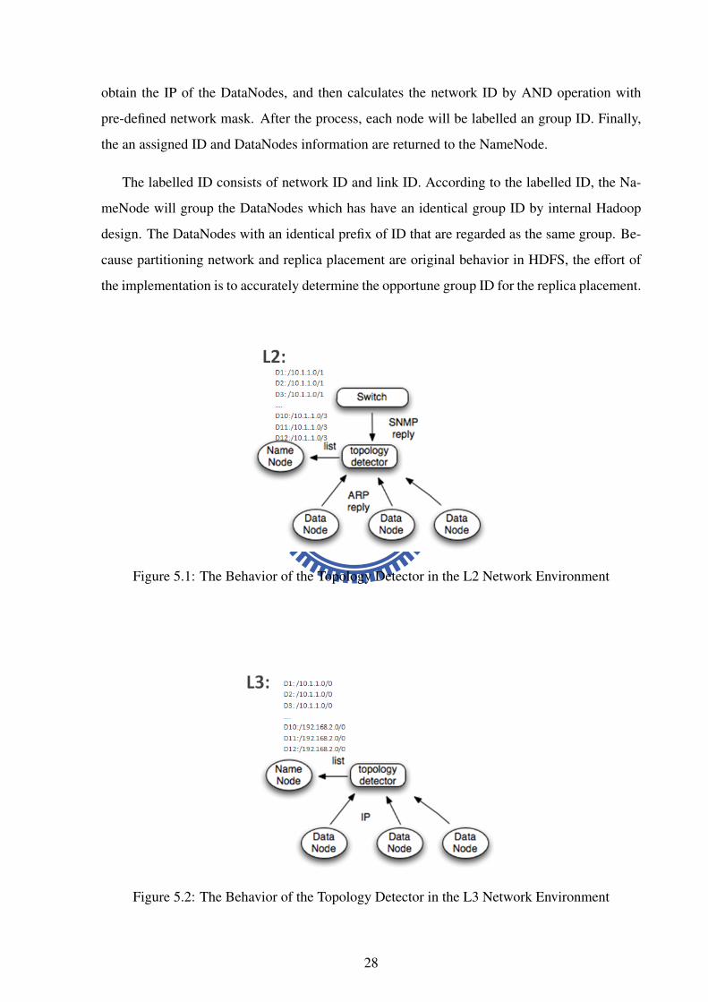
obtain the IP of the DataNodes, and then calculates the network ID by AND operation with

pre-defined network mask. After the process, each node will be labelled an group ID. Finally,

the an assigned ID and DataNodes information are returned to the NameNode.

The labelled ID consists of network ID and link ID. According to the labelled ID, the Na-

meNode will group the DataNodes which has have an identical group ID by internal Hadoop

design. The DataNodes with an identical prefix of ID that are regarded as the same group. Be-

cause partitioning network and replica placement are original behavior in HDFS, the effort of

the implementation is to accurately determine the opportune group ID for the replica placement.

Figure 5.1: The Behavior of the Topology Detector in the L2 Network Environment

Figure 5.2: The Behavior of the Topology Detector in the L3 Network Environment

28

5.1.2 Compressor

Figure 5.3: The Design of Compressor

The compressor is designed to run in the background, and decompresses blocks n in time on

client side rather than DataNodes. As Figure 5.3 shows, for obtaining better performance, nei-

ther client’s decompression or the DataNodes’ compression are via JNI (Java Native Interface)

to combine LZO C library. So the client determines the data whether to read directly or read

with decompressing. The judgement of decompressing is based on the NameNode’s memory

whose contains a map for recording blocks location. We add a field to the map for flagging a

block if the block is compressed. The compressor is integrated into HDFS shell command. It

provides users with some flexible options.

Execution Command

"-t n" indicates the file or directory how long is not be accessed time. Typically, the file which

has not been accessed for a long time that has lower probability of being used in the

future.

"-r n" specifies how many replica should be compressed. To increase performance or save

space, the option is a trade off.

"-R" recursive to compress or decompress files

29

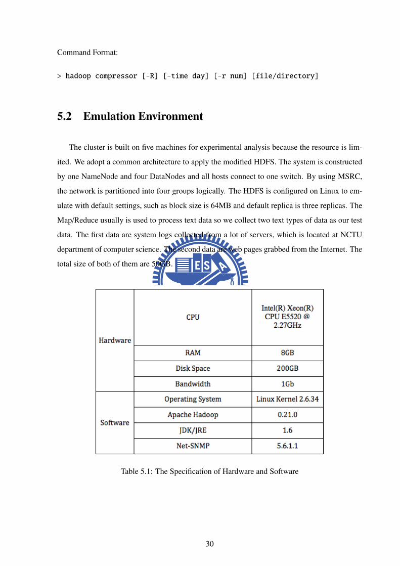
Command Format:

> hadoop compressor [-R] [-time day] [-r num] [file/directory]

5.2 Emulation Environment

The cluster is built on five machines for experimental analysis because the resource is lim-

ited. We adopt a common architecture to apply the modified HDFS. The system is constructed

by one NameNode and four DataNodes and all hosts connect to one switch. By using MSRC,

the network is partitioned into four groups logically. The HDFS is configured on Linux to em-

ulate with default settings, such as block size is 64MB and default replica is three replicas. The

Map/Reduce usually is used to process text data so we collect two text types of data as our test

data. The first data are system logs collected from a lot of servers, which is located at NCTU

department of computer science. The second data are web pages grabbed from the Internet. The

total size of both of them are 50GB.

Table 5.1: The Specification of Hardware and Software

30

5.3 Evaluation Criteria

For analyzing the study, there are three evaluation criteria to measure the result such as disk

space, compression time and access performance.

5.3.1 Disk Space

Figure 5.4: The Comparison of Saved Space with Different Data

Figure 5.4 shows, the data of system log can save 56% disk space, and the data of web

page is about 40%. The reason of system logs is better than web pages is the compression

ratio depends how many duplicated keyword in the data. So, system logs usually have such

duplicated vocabularies that it can be compressed with high ratio. As for web page, the size of

files is very small. The number of duplicated keyword in web pages is limited. So, saved space

on the web pages is less than the saved space on the system logs. Because of the size of data

may affect the number of duplicated keyword, we run a compression test with different block

size. But, the result shows the block size has no effect.

However, binary files almost have the worst compression ratio and will not reduce the con-

sumption of disk space. The files is not suitable to be compressed due to its file characteristics.

In current use of Hadoop, the most applications used for text processing, because the data which

processed by MapReduce, must can be divided for distributed computing. The characteristics

of data that limits the application on Hadoop. Nevertheless, MSRC is still very suitable to deal

with storing text files.

31

5.3.2 Compression Time

Figure 5.5: Comparing the Compression Time of System Logs and Web Pages

The Figure 5.5 shows, the large smaller file will spend more time for replica compression.

The major reason is that before to make compressing replicas of the blocks, the client asks the

NameNode for the location of the blocks. Because only a single NameNode replies the request

and the files consume too much memory, the response time causes the compression time longer.

Thus, the action of compressing runs in the background. Executing the compressor is best as

the system is at off-peak hours.

5.3.3 Performance of Reading Data

Figure 5.6: Performance of Reading Data

Figure 5.6 shows, when the DataNode crashed, the transmission time is reduced. The reason

32

is partial data which is read by using decompressing blocks in time. The size of transmitted

data is such very smaller than the original data that to accelerate the data transmission. Due to

compression algorithm is lightweight and decompression is fast, spending a few CPU resources

to tolerate server failure is very cost-effective.

5.4 Comparison

From Table 5.7, the minimum overhead of MSRC is about 1.5 times the space of one replica.

In text-based data the result can close to DiskReduce. The text data are very suitable to do

compression in Hadoop because its content may have many duplicate words. The difference

between MSRC and DiskReduce is the design of MSRC provides user with specifying whether

the files should be compressed or not. As to load balancing and performance, MSRC does

not consider the happening of popular file. Because Hadoop is a storage for computing usage,

it is almost impossible that too many users access the identical files. Moreover, increasing the

number of copy is able to uniformly distribute replicas, but the improved performance is limited.

The main reason is computing power, which are composed of servers, is fixed.

Our study is very practical that using Hadoop to process large amount of data. Administrator

can arbitrarily adjust the resource according to files utilization. For keep data reliability, admin-

istrator do not deal with recoding the location of servers because the system will automatically

detect the DataNodes location.

Figure 5.7: The Compression to MSRC and the Studies

33

5.5 Issues

There are a few issues in regards to whether compressing all replicas, and space balancing.

We will discuss them in this section.

5.5.1 Compressing Entire Replicas versus Partial Replicas

The additional replicas whether always be compressed that is a trade off. Increasing replica

factor that come with high performance because the loading is shared onto the DataNodes

evenly. Moreover, The data availability of using many replicas is higher that a few replicas

in the system. But, the space is not always unlimited. The penalty of high replicas is the higher

overhead of the space. HDFS is not designed for general use such as FTP and HTTP. The us-

age of HDFS is only suitable for writing once and read many times. So, only considering the

system is for MapReduce computing purpose. There is no hot files because computed data are

not frequently shared among the users. Further, the probability of multiple users, which require

the same data to process, is very low. Replicas are compressed that can increase the speed of

block transmission via network because the blocks size is the smaller. But, Compressing and

decompressing replicas pays the penalty, which implies the Nodes that must spend computing

power rather than concentrating on MapReduce jobs. In our design, it has no extra CPU cost to

deal with compressing or decompressing replicas in normal time. When the DataNode crashs,

the client receives compressed replicas and then decompress it with few CPU consumption.

Processing the decompressed files is faster than compressing file, because the access speed of

the disk is much slower than memory and the compression algorithm we used that has a very

high decompression speed. Spending a few computing resource to do block compression that

can accelerate the speed of block transmission. But, when in a environment which has many

computed jobs, block compression is bound to cost some computing resource such that the

throughput of the jobs is down. So, we design a flexible option for users. The users can execute

a compression command according their computing utilization. They can also compress the

files which the partial users have, because their priority is lower, can also compress files with

old modification time because the access probability of files is lower.

34

5.5.2 The Difference Between Rack-based and Network-based

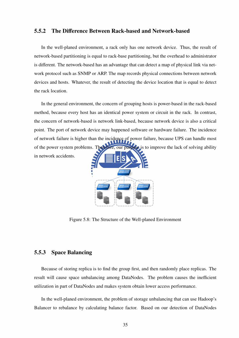
In the well-planed environment, a rack only has one network device. Thus, the result of

network-based partitioning is equal to rack-base partitioning, but the overhead to administrator

is different. The network-based has an advantage that can detect a map of physical link via net-

work protocol such as SNMP or ARP. The map records physical connections between network

devices and hosts. Whatever, the result of detecting the device location that is equal to detect

the rack location.

In the general environment, the concern of grouping hosts is power-based in the rack-based

method, because every host has an identical power system or circuit in the rack. In contrast,

the concern of network-based is network link-based, because network device is also a critical

point. The port of network device may happened software or hardware failure. The incidence

of network failure is higher than the incidence of power failure, because UPS can handle most

of the power system problems. Therefore, our purpose is to improve the lack of solving ability

in network accidents.

Figure 5.8: The Structure of the Well-planed Environment

5.5.3 Space Balancing

Because of storing replica is to find the group first, and then randomly place replicas. The

result will cause space unbalancing among DataNodes. The problem causes the inefficient

utilization in part of DataNodes and makes system obtain lower access performance.

In the well-planed environment, the problem of storage unbalancing that can use Hadoop’s

Balancer to rebalance by calculating balance factor. Based on our detection of DataNodes

35

location and Balancer function, the unbalancing possibility in most network environments is

very low. As Figure 5.9 shows, the result is acceptable that the chosen possibility of a host in the

first group is 1/4N. However, there is no solution to balance the worst environment with keeping

availability. Thus, we use a simple way to solve it that like HDFS’s balancer. The concept of

Figure 5.9: The Case for Space Unbalancing

the way is re-compressing the file. The current block map that shows one or two copies of block

are compressed. So, re-choosing replica to compress in the principle of balancing the space of

the node.

36

Chapter 6

Conclusion and Future Work

In this thesis, we proposed a management strategy of replica compression for improving data

reliability and saving disk space. Our method dynamically detects the topology of DataNodes

in any layer 2 and layer 3 network. That makes administrator no longer to manually maintain

a list for servers location, and the placement policy makes the files are always available even

nodes fail. Moreover, in the strategy the compressor compresses the additional replicas such

that storage reduced. The results demonstrate our work is effective in text-based computing

usage.

In the future, the compressor can integrate with other compression algorithm for various

situations. Usually, the access frequency of the third copy is less than the frequency time of the

second copy. Thus, it can consider to be compressed with high ratio compression algorithm so

the much space can be saved.

37

REFERENCE

[1] T. White, Hadoop: The Definitive Guide. O’Reilly Media, Yahoo! Press, June 5, 2009.

[2] J. Venner, Pro Hadoop. Apress, June 22, 2009

[3] K. Ranganathan, A. Iamnitchi, and I. Foste. Improving data availability through dynamic

model-driven replication in large peer-to-peer communities. In In 2nd IEEE/ACM Inter-

national Symposium on Cluster Computing and the Grid, pages 376381, 2002

[4] S. Ghemawat, H. Gobioff, and S.-T. Leung, "The google file system," SIGOPS Oper. Syst.

Rev., vol. 37, no. 5, pp. 29-43, 2003.

[5] J. Dean and S. Ghemawat, "MapReduce: Simplified Data Processing on Large Clusters,"

Proc. 6th Symp. Operating System Design and Implementation (OSDI), Usenix Assoc.,

2004, pp. 137-150.

[6] H. Lamehamedi, B. Szymanski, Z. Shentu, and E. Deelman, "Data replication strategies

in grid environments," in Proceedings of the Fifth International Conference on Algorithms

and Architectures for Parallel Processing. Press, 2002, pp. 378383.

[7] R.M Rahman, K Barker and R Alhajj, "Replica selection strategies in data grid", Journal

of Parallel and Distributed Computing, Volume 68, Issue 12, Pages 1561-1574, December

2008.

[8] B. Fan, W. Tantisiriroj, L. Xiao, and G. Gibson, "DiskReduce: RAID for data-intensive

scalable computing," in PDSW ’09: Proceedings of the 4th Annual Workshop on Petascale

Data Storage. New York, NY, USA: ACM, 2009, pp. 610.

38

[9] Q. Wei, B. Veeravalli, B. Gong, L. Zeng and D. Feng, "CDRM: A Cost-Effective Dy-

namic Replication Management Scheme for Cloud Storage Cluster," IEEE International

Conference on Cluster Computing, 2010, pp.188-196.

[10] K. Shvachko, H. Huang, S. Radia, and R. Chansler, "The hadoop distributed file system,"

in 26th IEEE (MSST2010) Symposium on Massive Storage Systems and Technologies,

May 2010.

[11] J. Leverich and C. Kozyrakis, "On the energy (in) efficiency of hadoop clusters," ACM

SIGOPS Operating Systems Review, vol. 44, no. 1, pp.6165, 2010.

[12] D. Borthakur, "The Hadoop Distributed File System: Architecture and Design," The

Apache Software Foundation, 2007.

[13] The Apache Software Foundation. Hadoop. http://hadoop.apache.org/core/, 2009 [Jun. 25,

2011].

[14] H. Kuang, "Rack-aware Replica Placement," https://issues.apache.org/jira/browse/HADOOP-

692, 2006 [Jun. 25, 2011]

[15] M. Oberhumer, "LZO - a real-time data compression library,"

http://www.oberhumer.com/opensource/lzo/, April 2008. [Jun. 25, 2011]

39