Tomi Kankkunen

Dynamic stress concentrations in unidirectional carbon fibre composites

School of engineering

Thesis submitted for examination for the degree of Master of

Science in Technology.

Espoo 30.09.2019

Thesis supervisor and advisor:

Prof. Luc St-Pierre

Aalto-yliopisto, PL 11000, 00076

AALTO

www.aalto.fi

Diplomityön tiivistelmä

Tekijä Tomi Kankkunen

Työn nimi Dynamic stress concentrations in unidirectional carbon fibre composites

Maisteriohjelma Konetekniikan maisteriohjelma Koodi ENG25

Työn valvoja Luc St-Pierre

Työn ohjaaja(t) Luc St-Pierre

Päivämäärä 30.09.2019 Sivumäärä 62 Kieli englanti

Tiivistelmä

Yhdensuuntaisilla hiilikuiduilla lujitettuja muovikomposiitteja käytetään vaativissa rakenteellisissa

sovellutuksissa, minkä vuoksi on tärkeää tuntea perusteellisesti komposiitin lujuus ja vaurion ke-

hittymismekanismit. Näitä mekanismeja ei tunneta vieläkään täysin, mikä johtaa ylimitoitettuihin,

tarpeettoman painaviin ja kalliisiin rakenteisiin. Eräs näistä mekanismeista on yhtenäistä säröä

muistuttava vierekkäisten hiilikuitusäikeiden katkeaminen samassa tasossa (samantasoinen klus-

teri), kun komposiitti on kuitujen suuntaisessa vetojännitystilassa. Havaintojen perusteella suurin

osa klustereista ovat samantasoisia. Loput klustereista taas muodostuvat niistä vierekkäisistä kui-

tusäikeiden katkeamiskohdista, jotka eivät ole samassa tasossa (hajaantunut klusteri), mikä johtuu

kuidun lujuuden tilastollisesta hajonnasta. Tämä havainto on ristiriidassa nykyaikaisten mallien

kanssa, jotka ennustavat, että suurin osa klustereista hajaantuu ja vain pieni osa on samantasoisia.

Lisäksi nykyisillä malleilla on vaikeuksia selittää samantasoisten klustereiden nopea kasvu ja siitä

seuraava komposiitin lopullinen murtuminen.

Tämän työn taustatarkoituksena on arvioida, johtuuko samantasoisten klusterien yleisyys kuitu-

säikeen katkeamisen aiheuttamasta dynaamisesta jännityksestä. Nykyaikaiset mallit eivät ole on-

nistuneet jäljittelemään katkeamiseen liittyviä kolmiulotteisia dynaamisia ilmiöitä. Sen sijaan ny-

kyiset mallit ovat rajoittuneet joko i) staattisiin jännityksiin tai ii) kaksiulotteisiin geometrioihin.

Tässä työssä dynaamiset jännitykset simuloidaan numeerisesti elementtimenetelmää (FEM) käyt-

täen laajentamalla erästä nykyaikaista kolmiulotteista staattista mallia. Dynaamisten jännitysten

suuruutta arvioidaan ensisijaisesti vertaamalla niitä vastaavaan jo olemassa olevaan malliin, joka

ottaa huomioon vain staattisen jännityksen. Lisäksi jännityksiä simuloidaan käyttäen erilaisia mal-

lin alkuasetuksia, muun muassa muuttaen katkeavien kuitujen määrää, täyteaineen materiaalimal-

lia sekä kuitupitoisuutta.

Simuloitujen tulosten pohjalta päädyttiin kolmeen päälopputulokseen. Ensiksi, täyteaineen mate-

riaalimallilla näyttäisi olevan merkittävä vaikutus dynaamiseen jännitykseen. Lineaari-elastinen

materiaalimalli johti huomattavasti suurempiin dynaamisiin jännityksiin kuin täysin plastinen

malli. Toisekseen, dynaamisten jännitysten merkitys kasvoi hieman, kun katkeavien kuitujen

määrä kasvoi. Kolmanneksi, kuitupitoisuuden lisäys pienensi dynaamisia jännityksiä rikkoutuneen

kuidun ympärillä. Kaiken kaikkiaan, dynaamiset jännitykset olivat vähintään hieman suurempia

kuin staattiset jännitykset. Vaikka tulosten pohjalta on vielä haastavaa selittää nykyinen samanta-

soisten klusterien muodostuminen, tämä tutkimus luo pohjan tutkia ilmiötä tarkemmin muun

muassa eri parametreja muuttamalla.

Avainsanat dynaaminen murtuminen, elementtimenetelmä, hiilikuitu, lujitemuovi, sa-

mantasoinen murtuma, yhdensuuntaiskuitu

Aalto University, P.O. BOX 11000, 00076 AALTO

www.aalto.fi

Abstract of master's thesis

Author Tomi Kankkunen

Title of thesis Dynamic stress concentrations in unidirectional carbon fibre composites

Master programme Master's Programme in Mechanical

Engineering

Code ENG25

Thesis supervisor Luc St-Pierre

Thesis advisor(s) Luc St-Pierre

Date 30.09.2019 Number of pages 62 Language English

Abstract

Unidirectional (UD) carbon fibre reinforced polymer (CFRP) composites are applied in demanding structural applications. Therefore, it is extremely beneficial to be able to estimate the strength and damage development mechanisms of the CFRP structure. Currently, these mechanisms are not known completely, which leads to overdesigned and unnecessarily heavy expensive structures. One of these damage development mechanisms is the formation of co-planar clusters of broken fibres during the tensile loading. When UD CFRP is loaded in tension, fibre filaments start breaking at some point. Most of these fibre breaks form a crack-like shape, i.e. a co-planar cluster, and the other breaks diffuse around the break point. However, current models fail to predict this observed prevalence of co-planar clusters. Moreover, the current models have difficulties to explain the rapid growth of these co-planar cracks, and consequently, to predict the final failure of the compo-site. This thesis attempts to explain the formation of co-planar clusters by incorporating dynamic stresses in the current state-of-art models. There are currently no models that could capture 3-dimensional dynamic behaviour in UD composite. Instead, current models are either limited to i) static stresses or ii) 2-dimensional geometries. The dynamic stresses are obtained numerically via a finite element method (FEM) by extending an existing 3-dimensional static model. The significance of dynamic stresses is primarily determined by comparing the dynamic and static stresses for the same model setup. Dynamic stresses are simulated by varying input parameters, including the number of breaking fibres, matrix material model and fibre volume fraction. The analysis of results produced three main conclusions. Firstly, the material model of the matrix has a significant effect on the dynamic stresses. Modelling matrix as a linear elastic led to signifi-cantly higher dynamic stresses than perfectly plastic matrix. Secondly, dynamic stresses become more important when the number of breaking fibres increases. Thirdly, the increase of volume fraction decreases slightly the dynamic stresses. Overall, the results consistently showed that dy-namic stresses will at least slightly increase the probability of co-planar crack formation. Further studies with modified setups would obtain important additional data for dynamic behaviour of the composite.

Keywords carbon fibre, co-planar cluster, dynamic break, finite element method, poly-

mer composite, unidirectional

Foreword

The thesis was written to further develop the numerical study ‘Stress redistribution

around clusters of broken fibres in a composite’ conducted by Luc St-Pierre and his

group. The background motivation of the thesis was the need to develop strength predic-

tions in carbon fibre composites. One of the factors that decrease the reliability of the

current strength predictions is the challenge to predict and explain the observed co-pla-

nar cluster formation.

I would like to thank my advisor and supervisor Luc St-Pierre for his insightful, sharp-

eyed advice and persevering support thorough the process. It was extremely rewarding

to have these numerous in-depth discussion hours with you. I would also like to thank my

wife for her encouraging comments, help with practical issues and endless faith in me.

Not forgetting my family and friends who taught me to laugh during the moments of des-

pair. Thank you all, this has been a memorable journey.

Espoo 30.9.2019

Tomi Kankkunen

1

Table of contents Symbols ............................................................................................................................. 2 1 Introduction ............................................................................................................... 4 2 Literature review ....................................................................................................... 7

2.1 Overview of unidirectional composite ............................................................... 7 2.1.1 Geometry and packing ................................................................................ 7

2.1.2 Static structural analysis of intact composite .............................................. 9 2.1.3 Failure development of unidirectional composite ..................................... 10 2.1.4 Material models of matrix ......................................................................... 13 2.1.5 Stiffness and strength of a fibre filament .................................................. 14

2.2 Static analysis of a broken composite .............................................................. 16

2.2.1 Static stress concentration factor ............................................................... 16 2.2.2 Static SCF including matrix plasticity ...................................................... 21

2.2.3 Static stress redistribution along the fibre ................................................. 23

2.2.4 Static SCF via finite element modelling ................................................... 24 2.3 Dynamic analysis of broken UD composite ..................................................... 25

2.3.1 Dynamic stress propagation ...................................................................... 25 2.3.2 Dynamic stress concentration factor ......................................................... 27

2.3.3 Dynamic SCF along the intact fibre .......................................................... 30 2.3.4 Dynamic SCF via finite element modelling .............................................. 32

2.4 SCF summary ................................................................................................... 34 3 Dynamic finite element model ................................................................................ 36

3.1 Model description ............................................................................................. 36 3.1.1 Geometry and mesh................................................................................... 36 3.1.2 Boundary conditions ................................................................................. 37

3.1.3 Material modelling .................................................................................... 40

3.2 Model calibration ............................................................................................. 40 3.2.1 Step time calibration ................................................................................. 43 3.2.2 Model length calibration ........................................................................... 45

3.2.3 Mesh parameter calibration ....................................................................... 46 3.2.4 Variation of remote stress ......................................................................... 47

4 Results and discussion ............................................................................................ 49 4.1 Effect of number of broken fibres .................................................................... 49 4.2 Fibres breaking in a row ................................................................................... 51 4.3 Effect of fibre volume fraction ......................................................................... 52

4.4 Discussion ........................................................................................................ 53 4.4.1 Input data ................................................................................................... 53 4.4.2 Modelling aspects...................................................................................... 54

5 Conclusions ............................................................................................................. 56

References ....................................................................................................................... 58

2

Symbols

𝐴 cross-sectional area of composite 𝐶 shear lag perimeter 𝐶∗ integration region 𝐸 tensile modulus 𝐸𝑓 tensile modulus of fibre

𝐸𝑚 tensile modulus of matrix 𝐹 remote force on composite 𝐺 shear modulus 𝑃 remote force on fibres

𝑃𝑙𝑖𝑚𝑖𝑡 threshold remote force to cause matrix yielding

𝑃(𝜎𝑓) failure probability at 𝜎𝑓

𝐿0 reference gauge length 𝐿 length of the model / gauge length 𝑆 shear force in matrix 𝑉𝑓 volume fraction of fibres

𝑉𝑚 volume fraction of matrix 𝑈𝑓 tensile energy in fibre

𝑈𝑚 tensile energy in matrix 𝑎 size of the plastic zone in longitudinal direction 𝑐𝐿 longitudinal stress wave propagation speed

𝑐𝑠ℎ𝑒𝑎𝑟 transversal stress wave propagation speed 𝑑 surface-to-surface distance between adjacent fibres 𝑒𝑟 element size in radial direction 𝑒𝑡 element size in tangential direction 𝑒𝑥 element size in longitudinal direction 𝑘𝑑𝑦𝑛 dynamic stress concentration factor

𝑘𝑑𝑦𝑛∗ (𝑠∗) Laplace transform of dynamic stress concentration factor

ℎ effective longitudinal distance of matrix shearing 𝑖 imaginary unit 𝑙𝑒 recovery length 𝑚 Weibull modulus 𝑚𝑙 concentrated mass per unit length 𝑛𝑏 number of broken fibres 𝑛𝐿 element number in longitudinal direction 𝑛𝑟 element number in radial direction in a unit cell 𝑛𝑡 total number of fibres 𝑛𝑢 element number at the edge of a unit cell 𝑟𝑏 equivalent radii of broken bundle 𝑟𝑐 equivalent radii 𝑠 distance between centroids of adjacent fibres 𝑠∗ Laplace transform variable 𝑡 time variable 𝑡𝐿 longitudinal stress wave travel time

𝑡𝑠ℎ𝑒𝑎𝑟 transversal stress wave travel time 𝑡𝑡 total time of simulation

3

𝑡1 time period for stress state initiation (Step 1) 𝑡2 time period for post-release dynamics (Step 2) 𝑡∗ dimensionless time 𝑢 displacement in longitudinal direction 𝛼 static analytical model parameter 𝜖 normal strain in composite 𝜂𝑟 dynamic response factor 𝜆 static analytical model parameter 𝜈𝑚 Poisson’s ratio for matrix 𝜉 dimensionless coordinate in longitudinal direction 𝜌𝑓 mass density for fibre

𝜌𝑚 mass density for matrix 𝜎 normal stress in the longitudinal direction 𝜎𝑓 normal stress in fibre

𝜎𝑚 normal stress in matrix 𝜎∞ remote stress in fibre 𝜎0 scaling parameter for Weibull probability distribution 𝜏 shear stress 𝜏𝑦 shear yield strength of matrix

𝜙 fibre diameter

𝜕

𝜕𝑥 partial spatial derivative operator

𝜕

𝜕𝑡 partial temporal derivative operator

4

1 Introduction

Unidirectional (UD) carbon fibre reinforced polymer (CFRP) composites are known for

their excellent strength-to-weight ratio, high stiffness and customizability for different

structural applications. Over the last decades, they have constantly increased their market

share in engineering applications including civil, aerospace and automotive industries. In

order to reliably apply UD CFRP, it is crucial to understand key strength models and

damage development mechanisms in the structure. Profound understanding of these

mechanisms enables safe and effective use of material. For example, aerospace industry

demands safety and reliability, while sports industry looks for lightweight equipment. A

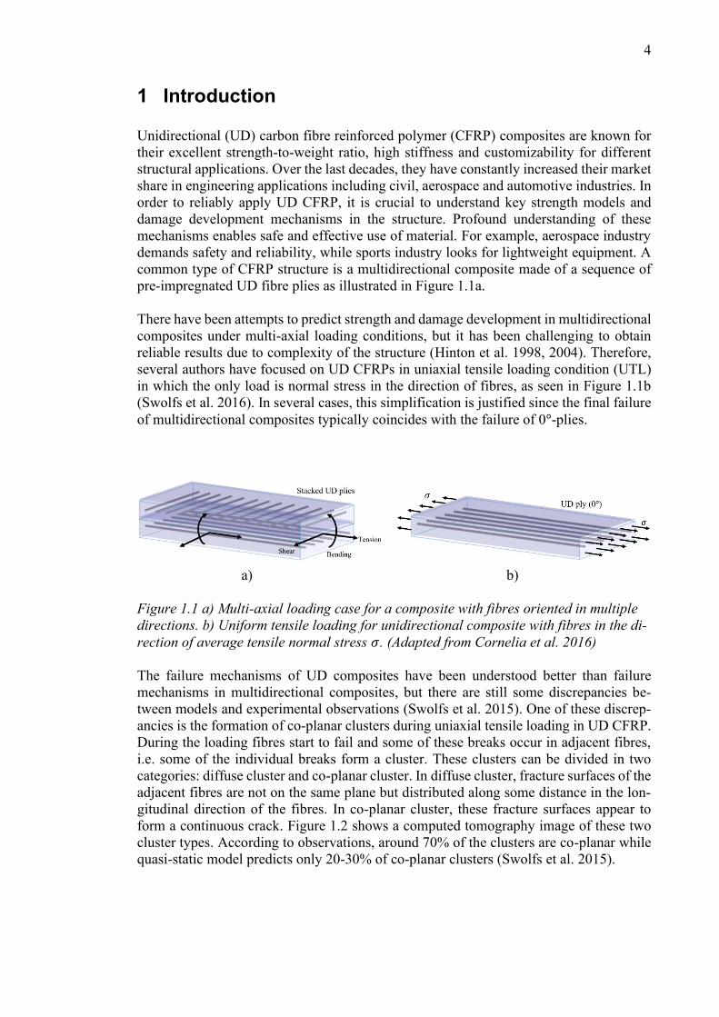
common type of CFRP structure is a multidirectional composite made of a sequence of

pre-impregnated UD fibre plies as illustrated in Figure 1.1a.

There have been attempts to predict strength and damage development in multidirectional

composites under multi-axial loading conditions, but it has been challenging to obtain

reliable results due to complexity of the structure (Hinton et al. 1998, 2004). Therefore,

several authors have focused on UD CFRPs in uniaxial tensile loading condition (UTL)

in which the only load is normal stress in the direction of fibres, as seen in Figure 1.1b

(Swolfs et al. 2016). In several cases, this simplification is justified since the final failure

of multidirectional composites typically coincides with the failure of 0°-plies.

a) b)

Figure 1.1 a) Multi-axial loading case for a composite with fibres oriented in multiple

directions. b) Uniform tensile loading for unidirectional composite with fibres in the di-

rection of average tensile normal stress 𝜎. (Adapted from Cornelia et al. 2016)

The failure mechanisms of UD composites have been understood better than failure

mechanisms in multidirectional composites, but there are still some discrepancies be-

tween models and experimental observations (Swolfs et al. 2015). One of these discrep-

ancies is the formation of co-planar clusters during uniaxial tensile loading in UD CFRP.

During the loading fibres start to fail and some of these breaks occur in adjacent fibres,

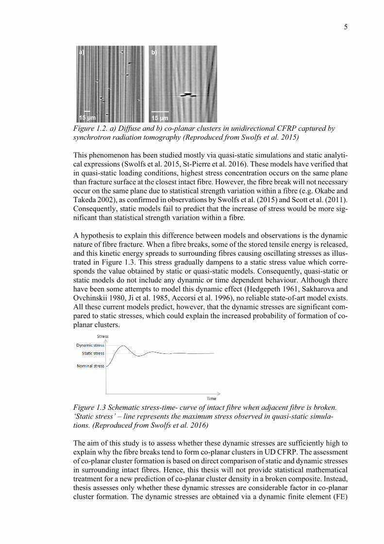
i.e. some of the individual breaks form a cluster. These clusters can be divided in two

categories: diffuse cluster and co-planar cluster. In diffuse cluster, fracture surfaces of the

adjacent fibres are not on the same plane but distributed along some distance in the lon-

gitudinal direction of the fibres. In co-planar cluster, these fracture surfaces appear to

form a continuous crack. Figure 1.2 shows a computed tomography image of these two

cluster types. According to observations, around 70% of the clusters are co-planar while

quasi-static model predicts only 20-30% of co-planar clusters (Swolfs et al. 2015).

5

Figure 1.2. a) Diffuse and b) co-planar clusters in unidirectional CFRP captured by

synchrotron radiation tomography (Reproduced from Swolfs et al. 2015)

This phenomenon has been studied mostly via quasi-static simulations and static analyti-

cal expressions (Swolfs et al. 2015, St-Pierre et al. 2016). These models have verified that

in quasi-static loading conditions, highest stress concentration occurs on the same plane

than fracture surface at the closest intact fibre. However, the fibre break will not necessary

occur on the same plane due to statistical strength variation within a fibre (e.g. Okabe and

Takeda 2002), as confirmed in observations by Swolfs et al. (2015) and Scott et al. (2011).

Consequently, static models fail to predict that the increase of stress would be more sig-

nificant than statistical strength variation within a fibre.

A hypothesis to explain this difference between models and observations is the dynamic

nature of fibre fracture. When a fibre breaks, some of the stored tensile energy is released,

and this kinetic energy spreads to surrounding fibres causing oscillating stresses as illus-

trated in Figure 1.3. This stress gradually dampens to a static stress value which corre-

sponds the value obtained by static or quasi-static models. Consequently, quasi-static or

static models do not include any dynamic or time dependent behaviour. Although there

have been some attempts to model this dynamic effect (Hedgepeth 1961, Sakharova and

Ovchinskii 1980, Ji et al. 1985, Accorsi et al. 1996), no reliable state-of-art model exists.

All these current models predict, however, that the dynamic stresses are significant com-

pared to static stresses, which could explain the increased probability of formation of co-

planar clusters.

Figure 1.3 Schematic stress-time- curve of intact fibre when adjacent fibre is broken.

‘Static stress’ – line represents the maximum stress observed in quasi-static simula-

tions. (Reproduced from Swolfs et al. 2016)

The aim of this study is to assess whether these dynamic stresses are sufficiently high to

explain why the fibre breaks tend to form co-planar clusters in UD CFRP. The assessment

of co-planar cluster formation is based on direct comparison of static and dynamic stresses

in surrounding intact fibres. Hence, this thesis will not provide statistical mathematical

treatment for a new prediction of co-planar cluster density in a broken composite. Instead,

thesis assesses only whether these dynamic stresses are considerable factor in co-planar

cluster formation. The dynamic stresses are obtained via a dynamic finite element (FE)

6

model which extends from the quasi-static FE model made by St-Pierre et al. (2017) to

perform dynamic calculations. The FE model assumes that fibres are regularly packed

and ideally unidirectional.

The remainder of the thesis is divided in four main chapters. Chapter 2 overviews UD

CFRP composites and their properties. In addition, it presents the failure mechanisms of

the composite and introduces the commonly used analytical and numerical approaches to

determine stress redistribution near the broken fibre. These approaches include both static

and dynamic analyses, and the emphasis is on the results retrieved from the literature.

Chapter 3 presents in detail the dynamic numerical model implemented in the thesis. The

model uses the dynamic explicit finite element method (FEM) in Abaqus/CAE 2017 soft-

ware to obtain the dynamic caused by the breakage. In addition, the chapter shows the

systematic calibration and validation process of the model. Chapter 4 compares FE anal-

ysis results to existing analytical dynamic stress models and the results of the correspond-

ing quasi-static analysis. Finally, chapter 5 summarizes the conclusions and proposes fu-

ture actions for this research field.

7

2 Literature review

The literature review on (UD) carbon fibre reinforced polymer (CFRP) composites is di-

vided in three main sections. First section concentrates on overview, experimental data

and material modelling of UD composites. Second section presents and compares differ-

ent static models, and the third section presents the existing dynamic models. Static mod-

els have a rather significant weight in the literature review since current dynamic models

are simple and limited. While first section concentrates more on input data, second and

third sections focus on models obtaining the stresses following the fracture.

2.1 Overview of unidirectional composite

This section gives an overview of UD composites including geometry, simplified struc-

tural analysis, experimental observations and material properties. Firstly, it presents the

structure of UD composite with essential geometric parameters. Then it determines the

response of different components of UD composite in unidirectional tensile loading

(UTL). After that, it presents the failure development of UD composite. Finally, it pre-

sents essential material properties, including both experimental data and material model-

ling.

2.1.1 Geometry and packing

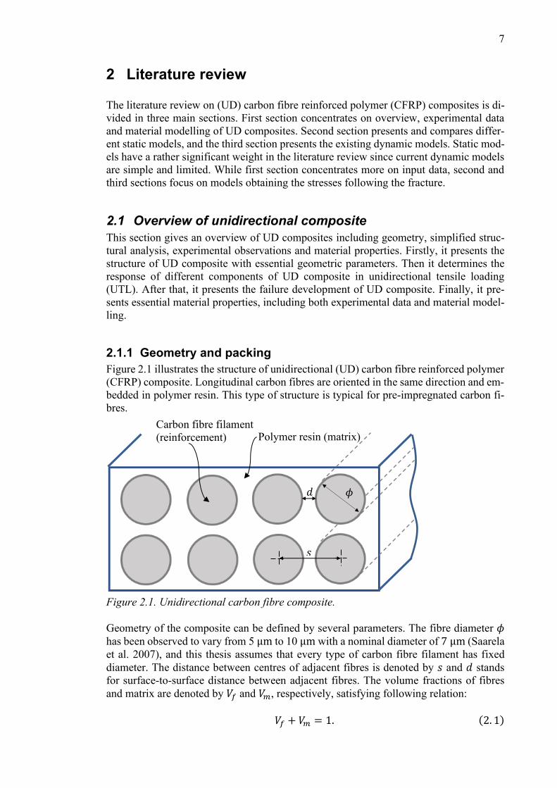
Figure 2.1 illustrates the structure of unidirectional (UD) carbon fibre reinforced polymer

(CFRP) composite. Longitudinal carbon fibres are oriented in the same direction and em-

bedded in polymer resin. This type of structure is typical for pre-impregnated carbon fi-

bres.

Figure 2.1. Unidirectional carbon fibre composite.

Geometry of the composite can be defined by several parameters. The fibre diameter 𝜙

has been observed to vary from 5 μm to 10 μm with a nominal diameter of 7 μm (Saarela

et al. 2007), and this thesis assumes that every type of carbon fibre filament has fixed

diameter. The distance between centres of adjacent fibres is denoted by 𝑠 and 𝑑 stands

for surface-to-surface distance between adjacent fibres. The volume fractions of fibres

and matrix are denoted by 𝑉𝑓 and 𝑉𝑚, respectively, satisfying following relation:

𝑉𝑓 + 𝑉𝑚 = 1. (2. 1)

𝜙 𝑑

𝑠

Polymer resin (matrix) Carbon fibre filament

(reinforcement)

8

In addition, in the case of regular square packed composite, following relation holds for

𝑉𝑓 and 𝑑:

𝑉𝑓 =𝜋𝜙2

4(𝑑 + 𝜙)2. (2. 2)

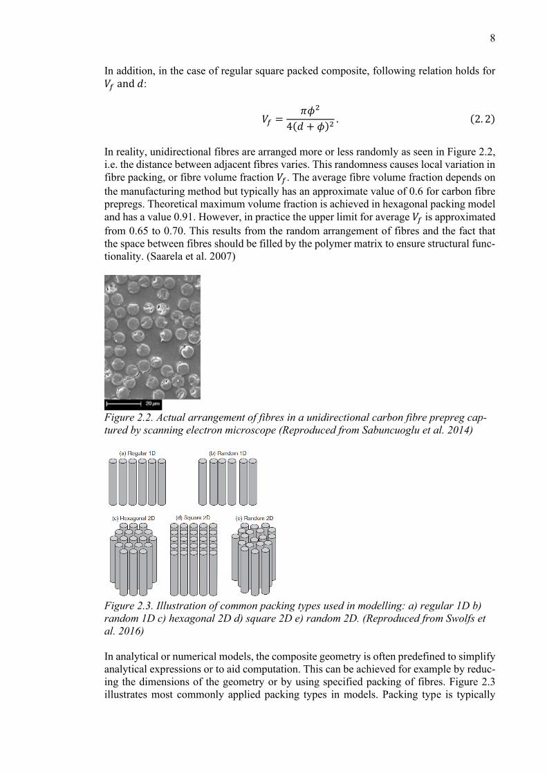
In reality, unidirectional fibres are arranged more or less randomly as seen in Figure 2.2,

i.e. the distance between adjacent fibres varies. This randomness causes local variation in

fibre packing, or fibre volume fraction 𝑉𝑓. The average fibre volume fraction depends on

the manufacturing method but typically has an approximate value of 0.6 for carbon fibre

prepregs. Theoretical maximum volume fraction is achieved in hexagonal packing model

and has a value 0.91. However, in practice the upper limit for average 𝑉𝑓 is approximated

from 0.65 to 0.70. This results from the random arrangement of fibres and the fact that

the space between fibres should be filled by the polymer matrix to ensure structural func-

tionality. (Saarela et al. 2007)

Figure 2.2. Actual arrangement of fibres in a unidirectional carbon fibre prepreg cap-

tured by scanning electron microscope (Reproduced from Sabuncuoglu et al. 2014)

Figure 2.3. Illustration of common packing types used in modelling: a) regular 1D b)

random 1D c) hexagonal 2D d) square 2D e) random 2D. (Reproduced from Swolfs et

al. 2016)

In analytical or numerical models, the composite geometry is often predefined to simplify

analytical expressions or to aid computation. This can be achieved for example by reduc-

ing the dimensions of the geometry or by using specified packing of fibres. Figure 2.3

illustrates most commonly applied packing types in models. Packing type is typically

9

divided in two main categories: 1D- and 2D-packing. 1D-packed models were imple-

mented in studies mainly from 60’s to 80’s (Hedgepeth 1961, Ji et al. 1985) while 2D-

packed models have been researched more recently as computational resources have im-

proved. It is also justified to move towards 2D-packed models since they appear to be

more representative of the physical nature of UD composites than models with 1D pack-

ing (van den Heuvel 1998, 2004).

Besides using different packing dimensions, researchers have utilized both randomly and

regularly packed fibres. Most of the research have focused on models with regular square

or hexagonal packing which enables more comparable and systematic study on UD com-

posites than models with random packing. Based on the current knowledge, the use of

regular packing can be justified in several cases. Some of the packings have features of

both regular and random packing in which one or more fibres are manually relocated to

distort the regular packing pattern (Landis and McMeeking 1999). (Swolft et al, 2016)

Other geometric parameters to model are number of fibres and fibre alignment. Analytical

models are typically applicable for infinite number of fibres. However, number of fibres

must be restricted in numerical models, such as in finite element model, to enable reason-

able computation time. Considering numerical models, St-Pierre et al. (2017) used up to

900 fibres while Swolfs et al. (2015) used 5500 fibres. However, more detailed models

may use around 100 fibres (Swolfs et al. 2013) or even only 1 to 10 fibres (e.g. Accorsi

et al. 1996, Heuvel et al. 2004). In many cases, this restriction is justified. Fibre alignment

is rarely taken into account in models, while measurements reveal fibre misalignments up

to a few degrees even with careful manufacturing. Instead, majority of the models assume

that all fibres are oriented in the same direction. The importance of this fibre misalign-

ment is still an open question. (Swolfs et al. 2016)

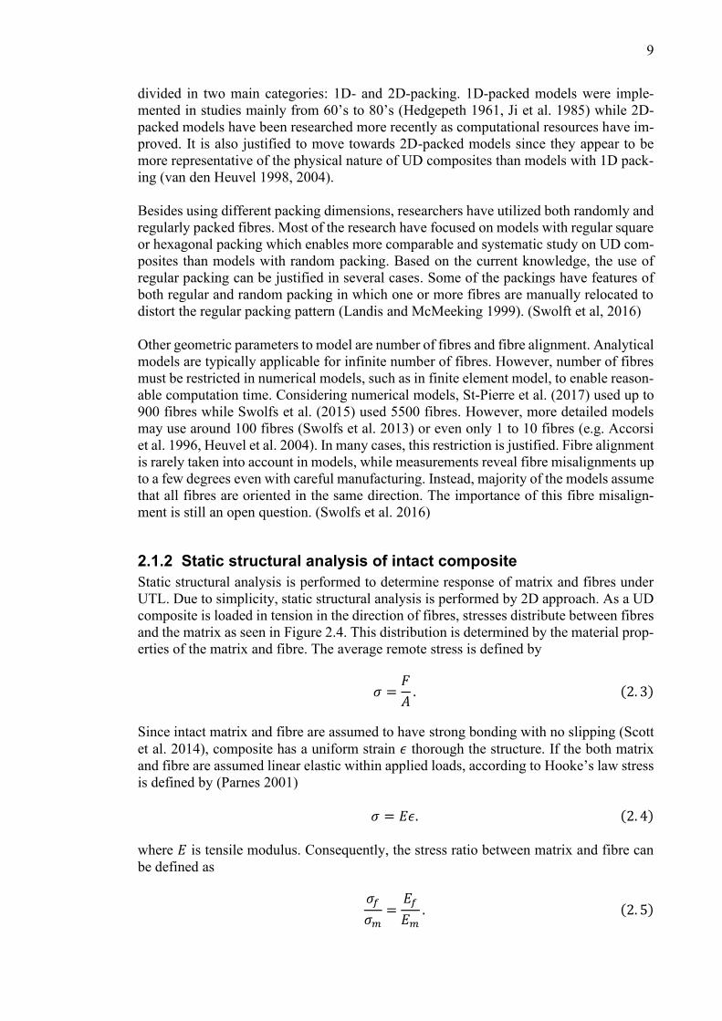
2.1.2 Static structural analysis of intact composite

Static structural analysis is performed to determine response of matrix and fibres under

UTL. Due to simplicity, static structural analysis is performed by 2D approach. As a UD

composite is loaded in tension in the direction of fibres, stresses distribute between fibres

and the matrix as seen in Figure 2.4. This distribution is determined by the material prop-

erties of the matrix and fibre. The average remote stress is defined by

𝜎 =𝐹

𝐴. (2. 3)

Since intact matrix and fibre are assumed to have strong bonding with no slipping (Scott

et al. 2014), composite has a uniform strain 𝜖 thorough the structure. If the both matrix

and fibre are assumed linear elastic within applied loads, according to Hooke’s law stress

is defined by (Parnes 2001)

𝜎 = 𝐸𝜖. (2. 4)

where 𝐸 is tensile modulus. Consequently, the stress ratio between matrix and fibre can

be defined as

𝜎𝑓

𝜎𝑚=𝐸𝑓

𝐸𝑚. (2. 5)

10

If fibre and matrix elements can be considered further as individual isotropic bar ele-

ments, the stored tensile energy per unit width is defined by (Parnes 2001)

𝑈𝑚 =𝜎𝑚2

2𝐸𝑚𝐴𝑉𝑚 and 𝑈𝑓 =

𝜎𝑓2

2𝐸𝑚𝐴𝑉𝑓 , (2. 6)

which leads to the energy ratio defined by

𝑈𝑓

𝑈𝑚=𝐸𝑓𝑉𝑓

𝐸𝑚𝑉𝑚. (2. 7)

Figure 2.4. Stress distribution in intact UD composite in tension (0°-ply).

Considering CFRP with material and structural properties of T800H/3631 prepreg (St-

Pierre et al. 2017), i.e. 𝐸𝑓 = 294 GPa, 𝐸𝑚 = 3 GPa and 𝑉𝑓 = 0.6, the resulting stress ratio

is 98. Similarly, the energy ratio has a value of 147. This indicates that fibres carry over

99 percent of the loads and stores over 99 percent of the tensile energy when composite

is loaded. Besides, normal stress in fibres is 98 times higher than in matrix. From this we

may further implicate that the stress and stored energy in matrix is relatively very small

when a composite is intact. On the other hand, matrix has a negligible contribution when

UD composite is intact. In the following chapters, 𝜎∞ will denote the remote stress in a

fibre.

2.1.3 Failure development of unidirectional composite

When the load on intact composite increases, weakest parts of the structure begin to fail.

As illustrated in Figure 1.1a in chapter 1, the actual composite may consist of several

layers of unidirectional carbon fibre layers. For example, Swolfs (2015), Scott (2011) and

co-workers performed an experiment on a multidirectional ply composite with some fibre

layers oriented along the tensile loading (0°-plies) and others aligned transversal to load-

ing (90°-plies). This implies that mechanical properties of this multidirectional composite

differ from purely unidirectional composite (Saarela et al. 2007). However, they observed

that before any breaks in 0°-plies, 90°-plies began to delaminate from the 0°-ply layers

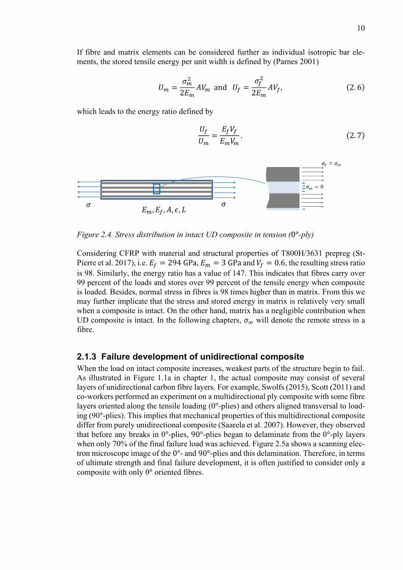
when only 70% of the final failure load was achieved. Figure 2.5a shows a scanning elec-

tron microscope image of the 0°- and 90°-plies and this delamination. Therefore, in terms

of ultimate strength and final failure development, it is often justified to consider only a

composite with only 0° oriented fibres.

𝜎 𝜎

𝐸𝑚, 𝐸𝑓 , 𝐴, 𝜖, 𝐿

11

a) d)

Figure 2.5 a) Cross section of a carbon fibre prepreg with stacked 0°- and 90°-plies at

94% of the failure load. Delamination between 0°- and 90°-plies occurred already at 70%

of the failure load. (Adapted from Swolfs et al. 2015). 2D slice views in UD ply showing

co-planar clusters of b) 3 c) 5 and d) 14 breaks. (Adapted from Scott et al. 2011)

When load is sufficiently large, failures begin to occur in the 0°-ply. First, weakest fibres

begin to fail forming individual breaks, which is expected due to statistical variation in

the strength of a fibre discussed more in chapter 2.1.5. As the loading increases further,

the breaks begin to concentrate close each other in adjacent fibres. These concentrated

breakages are called clusters. As the loading increases even further, larger clusters will

appear. Eventually the cluster size will be sufficiently large to cause unstable failure of

the whole composite due to rapid growth or formation of clusters. Swolfs (2015), Scott

(2011) and co-workers observed that at the 94% of the failure load, composite had a max-

imum cluster size of 14. Figure 2.5b, c and d show co-planar clusters of size 3, 5 and 14

breaks. Observations of cluster formation at the last 5% of the failure load has been dif-

ficult due to rapid fracture development and variations on strength of the composite (Scott

et al. 2011).

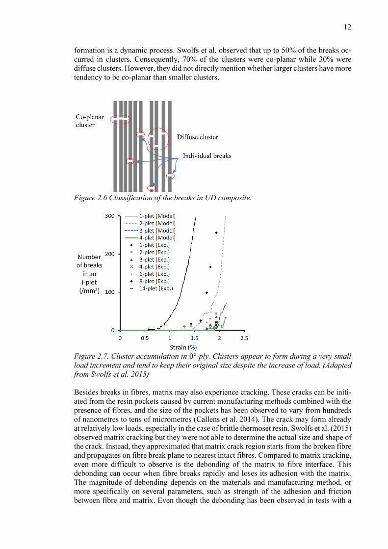
Generally, the fibre breaks in the UD composite can be distinguished to individual breaks

and clusters. According to Swolfs et al. (2015), a cluster is considered when axial distance

between breaks is less than five times fibre diameter 𝜙 and surface-to-surface distance

between breaks 𝑑 is less than diameter of fibre 𝜙. Clusters can be divided in two catego-

ries. If the axial distance is less than fibre radius 𝜙/2, cluster is categorised co-planar. If

not, cluster is categorised as a diffuse cluster. Figure 2.6 illustrates different cluster types

in random 1D packing.

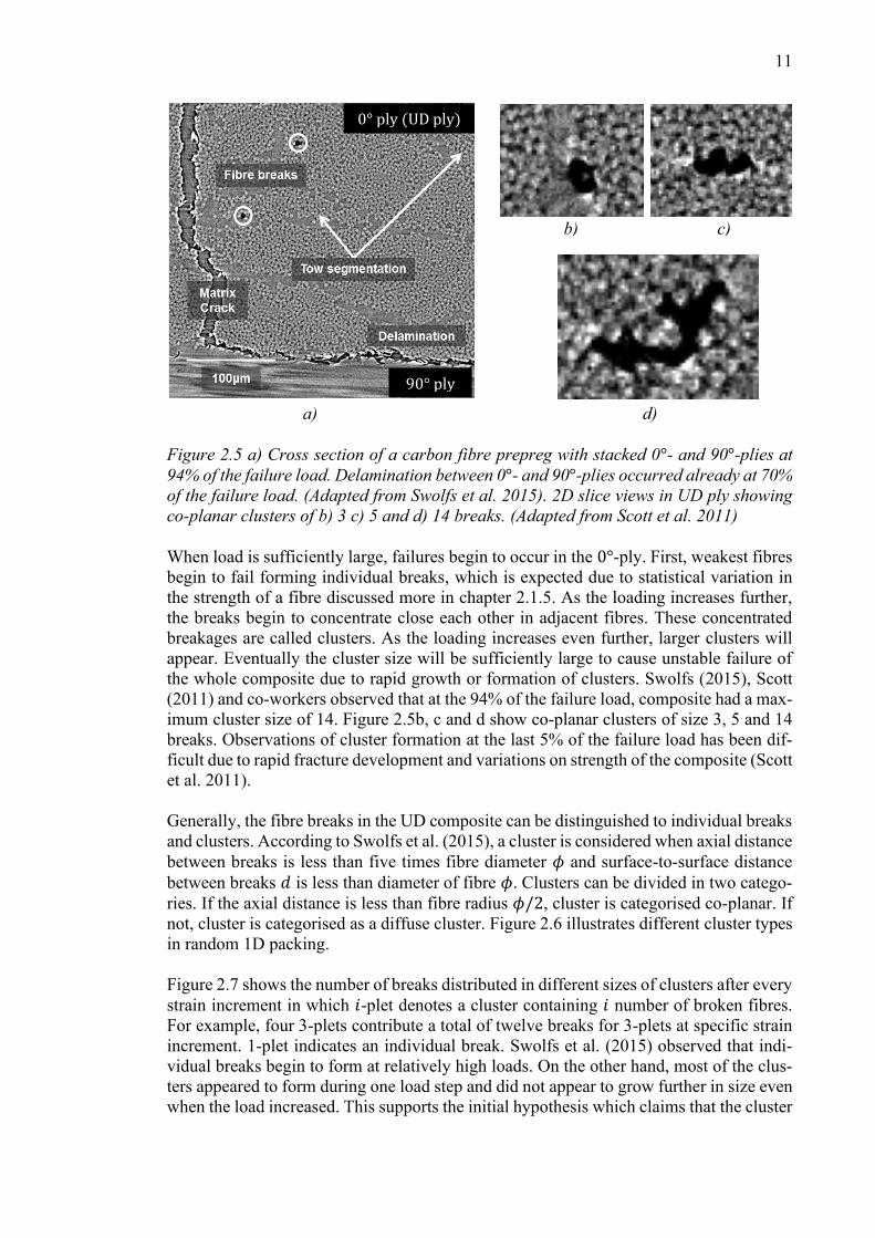
Figure 2.7 shows the number of breaks distributed in different sizes of clusters after every

strain increment in which 𝑖-plet denotes a cluster containing 𝑖 number of broken fibres.

For example, four 3-plets contribute a total of twelve breaks for 3-plets at specific strain

increment. 1-plet indicates an individual break. Swolfs et al. (2015) observed that indi-

vidual breaks begin to form at relatively high loads. On the other hand, most of the clus-

ters appeared to form during one load step and did not appear to grow further in size even

when the load increased. This supports the initial hypothesis which claims that the cluster

b) c)

0° ply (UD ply)

90° ply

12

formation is a dynamic process. Swolfs et al. observed that up to 50% of the breaks oc-

curred in clusters. Consequently, 70% of the clusters were co-planar while 30% were

diffuse clusters. However, they did not directly mention whether larger clusters have more

tendency to be co-planar than smaller clusters.

Figure 2.6 Classification of the breaks in UD composite.

Figure 2.7. Cluster accumulation in 0°-ply. Clusters appear to form during a very small

load increment and tend to keep their original size despite the increase of load. (Adapted

from Swolfs et al. 2015)

Besides breaks in fibres, matrix may also experience cracking. These cracks can be initi-

ated from the resin pockets caused by current manufacturing methods combined with the

presence of fibres, and the size of the pockets has been observed to vary from hundreds

of nanometres to tens of micrometres (Callens et al. 2014). The crack may form already

at relatively low loads, especially in the case of brittle thermoset resin. Swolfs et al. (2015)

observed matrix cracking but they were not able to determine the actual size and shape of

the crack. Instead, they approximated that matrix crack region starts from the broken fibre

and propagates on fibre break plane to nearest intact fibres. Compared to matrix cracking,

even more difficult to observe is the debonding of the matrix to fibre interface. This

debonding can occur when fibre breaks rapidly and loses its adhesion with the matrix.

The magnitude of debonding depends on the materials and manufacturing method, or

more specifically on several parameters, such as strength of the adhesion and friction

between fibre and matrix. Even though the debonding has been observed in tests with a

13

single fibre surrounded by matrix (Paipetis et al. 1999), it has been difficult to witness the

same phenomenon with an actual composite consisting of more than thousands of fibres

(Scott et al. 2014).

2.1.4 Material models of matrix

Considering UD CRFP matrix, the most crucial material properties are related to the

shearing of matrix. As shown later in chapters 2.2. and 2.3, shear deformation is most

essential deformation mechanism in matrix in a broken structure. In addition, tensile

strains in matrix are typically neglected in analytical models. Figure 2.8a shows measured

shear stress against shear strain on a bulk epoxy (Littell et al. 2008). Since actual stress

against strain relation is highly non-linear, the constitutive behaviour of matrix has been

simplified by various methods as seen in Figure 2.8b. Some of the applied constitutive

matrix models are:

1) Linear elastic (Hedgepeth 1961, Accorsi et al. 1996, Swolfs et al. 2015)

2) Non-linear elastic (Fiedler et al. 1998)

3) Linear elastic perfectly plastic (Hedgepeth and Van Dyke 1967, Blassiau et al.

2006, St-Pierre et al. 2017)

4) Linear elastic with strain hardening (Okabe and Takeda 2002)

a) b)

Figure 2.8 a) Measured shear stress versus shear strain for bulk epoxy matrix (Epon

E862) by varying strain rate (Adapted from Littell et al. 2008) b) Illustration of some

applied matrix material models

Contradict to actual measured data, models including plasticity have typically a specified

shear yield stress 𝜏𝑦. After exceeding that stress level, stresses behave in a linear manner.

For perfectly plastic model, 𝜏𝑦 represents maximum stress, but in model with linear strain

hardening, yield stress increases when strain has once exceeded this initial yield strain.

Although the real data reveals complex non-linear material behaviour, these piecewise

linear models are used to aid analysis or computation. Especially, linear elastic matrix

model is computationally efficient.

As Figure 2.6a shows, constitutive behaviour depends also on the strain rate. If shear load

is subjected with higher strain rate, matrix material appears to experience higher shear

stresses as Littell et al. (2008) observed during their tests on epoxy. Low strain rate cor-

responds the material behaviour for static models while high strain rates may occur during

dynamic loading. However, these tests are done for relatively large specimens for bulk

Shear strain

Shear stress

𝜏𝑦

linear elastic

non-linear elastic

linear elastic perfectly plastic

linear elastic with strain hardening

Increasing strain rate

Shear strain

14

epoxy while in the actual composite, space between fibres has a magnitude of a few mi-

crometres. In addition, the presence of fibres and the current manufacturing methods may

affect the molecular and microscale structure of polymer matrix. Hence, the constitutive

behaviour of matrix should be studied in microscale instead of relatively large macroscale

specimens. Microscale material properties are currently difficult to measure, and no data

exist in the literature. Therefore, due to uncertainties related to strain rate, microscale

material properties and measurement methods, one could consider several material mod-

els for the matrix. (Swolfs et al. 2016)

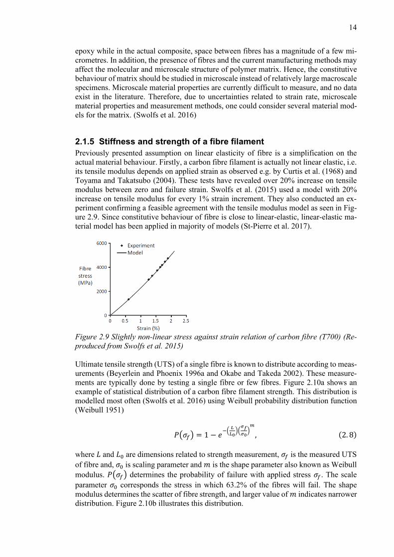
2.1.5 Stiffness and strength of a fibre filament

Previously presented assumption on linear elasticity of fibre is a simplification on the

actual material behaviour. Firstly, a carbon fibre filament is actually not linear elastic, i.e.

its tensile modulus depends on applied strain as observed e.g. by Curtis et al. (1968) and

Toyama and Takatsubo (2004). These tests have revealed over 20% increase on tensile

modulus between zero and failure strain. Swolfs et al. (2015) used a model with 20%

increase on tensile modulus for every 1% strain increment. They also conducted an ex-

periment confirming a feasible agreement with the tensile modulus model as seen in Fig-

ure 2.9. Since constitutive behaviour of fibre is close to linear-elastic, linear-elastic ma-

terial model has been applied in majority of models (St-Pierre et al. 2017).

Figure 2.9 Slightly non-linear stress against strain relation of carbon fibre (T700) (Re-

produced from Swolfs et al. 2015)

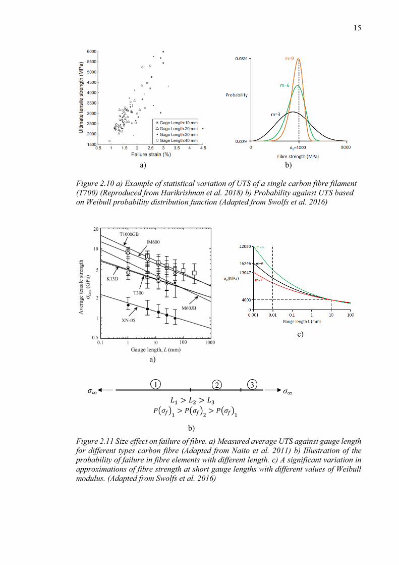
Ultimate tensile strength (UTS) of a single fibre is known to distribute according to meas-

urements (Beyerlein and Phoenix 1996a and Okabe and Takeda 2002). These measure-

ments are typically done by testing a single fibre or few fibres. Figure 2.10a shows an

example of statistical distribution of a carbon fibre filament strength. This distribution is

modelled most often (Swolfs et al. 2016) using Weibull probability distribution function

(Weibull 1951)

𝑃(𝜎𝑓) = 1 − 𝑒−(

𝐿

𝐿0)(𝜎𝑓

𝜎0)𝑚

, (2. 8)

where 𝐿 and 𝐿0 are dimensions related to strength measurement, 𝜎𝑓 is the measured UTS

of fibre and, 𝜎0 is scaling parameter and 𝑚 is the shape parameter also known as Weibull

modulus. 𝑃(𝜎𝑓) determines the probability of failure with applied stress 𝜎𝑓. The scale

parameter 𝜎0 corresponds the stress in which 63.2% of the fibres will fail. The shape

modulus determines the scatter of fibre strength, and larger value of 𝑚 indicates narrower

distribution. Figure 2.10b illustrates this distribution.

15

a) b)

Figure 2.10 a) Example of statistical variation of UTS of a single carbon fibre filament

(T700) (Reproduced from Harikrishnan et al. 2018) b) Probability against UTS based

on Weibull probability distribution function (Adapted from Swolfs et al. 2016)

Figure 2.11 Size effect on failure of fibre. a) Measured average UTS against gauge length

for different types carbon fibre (Adapted from Naito et al. 2011) b) Illustration of the

probability of failure in fibre elements with different length. c) A significant variation in

approximations of fibre strength at short gauge lengths with different values of Weibull

modulus. (Adapted from Swolfs et al. 2016)

𝑃(𝜎𝑓)1 > 𝑃(𝜎𝑓)2 > 𝑃(𝜎𝑓)1

𝐿1 > 𝐿2 > 𝐿3

1 2 3 𝜎∞

𝜎∞

c)

a)

b)

16

Measurements (Watson and Smith 1985, Langston 2016) indicate that the strength of the

fibre is sensitive to fibre length, or length of the gauge. If the gauge length is increased,

the strength of the fibre decreases. This decrease is caused by small defects in fibre; a

longer fibre is likely to have more defects, as illustrated in Figure 2.11a and b. Some of

these defects are more crucial than other ones which implicates that a longer fibre has

statistically more severe defect than a shorter one. Especially for high modulus fibres

these defects may be critical (Langston 2016). This results in lower expected strength in

some portion of the fibres.

State-of-art models would require measured data on very short gauge lengths. However,

there are some practical challenges. Watson and Smith (1985) have reported that reliable

measurements with gauge length below 1mm is complicated due to limitations of current

test methods. Currently fibre strength has been measured by gauge lengths approximately

from 1 mm to 50 mm, while some models would require measured data by only a few μm

gauge length to capture actual physical behaviour. Moreover, as shown later in chapter 3,

fibre elements in a finite element model have a length of even below 10 μm. Since reliable

statistical strength is not available for short gauge lengths, i.e. under 1 mm, many authors

are forced to extrapolate the strength for very short gauge lengths. As seen in Figure

2.11c, a gauge length of 1 μm causes a significant deviation in predicted strength although

Weibull modulus m is modified only by one unit. (Swolfs et al. 2016)

2.2 Static analysis of a broken composite

When some fibres have broken in a composite, stresses in broken fibres must be redis-

tributed to surrounding intact fibres. Since this thesis concentrates on co-planar clusters,

the analysis is performed considering fibre breaks in a same plane. Furthermore, the anal-

ysis assumes that only one cluster exists. In other words, intact fibres experience addi-

tional stresses contributed only by that one cluster, while in reality intact fibres might

experience stress increase caused by several clusters or fibre breaks (Beyerlein and Phoe-

nix 1996b). The analysis of static stress redistribution in broken structure emphasizes 2D

square packing, especially the work of St-Pierre et al. (2017), since the numerical model

of this thesis utilizes similar packing method.

First subsection focuses on static SCF obtained via different approaches and packings. It

compares the static SCF for hexagonal and square packed models and discusses of the

differences of the approaches. Second subsection assesses the effect of matrix plasticity.

Third subsection studies SCFs along the broken and intact fibre. Fourth subsection pre-

sents results from advanced models conducted via a finite element method.

2.2.1 Static stress concentration factor

Most important term to describe the increase of the stress, is stress concentration factor

(SCF). It describes the ratio of highest stress in specific fibre and remote stress and it is

defined generally by

SCF =𝜎𝑚𝑎𝑥 𝜎∞

. (2. 9)

Hedgepeth and Van Dyke (1967) were the first ones to obtain static stress concentration

in 2D packed fibre bundles. Figure 2.12 shows the geometry and configuration of the

broken bundle. Each fibre is loaded remotely via normal force 𝑃 and denoted by indices

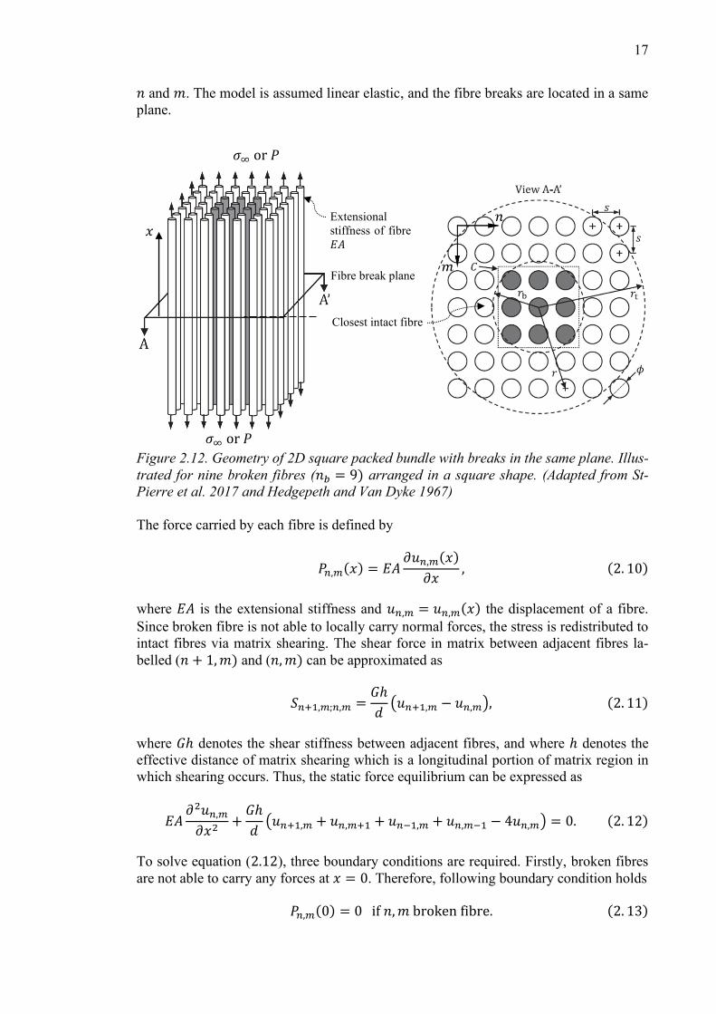
17

𝑛 and 𝑚. The model is assumed linear elastic, and the fibre breaks are located in a same

plane.

Figure 2.12. Geometry of 2D square packed bundle with breaks in the same plane. Illus-

trated for nine broken fibres (𝑛𝑏 = 9) arranged in a square shape. (Adapted from St-

Pierre et al. 2017 and Hedgepeth and Van Dyke 1967)

The force carried by each fibre is defined by

𝑃𝑛,𝑚(𝑥) = 𝐸𝐴𝜕𝑢𝑛,𝑚(𝑥)

𝜕𝑥, (2. 10)

where 𝐸𝐴 is the extensional stiffness and 𝑢𝑛,𝑚 = 𝑢𝑛,𝑚(𝑥) the displacement of a fibre.

Since broken fibre is not able to locally carry normal forces, the stress is redistributed to

intact fibres via matrix shearing. The shear force in matrix between adjacent fibres la-

belled (𝑛 + 1,𝑚) and (𝑛,𝑚) can be approximated as

𝑆𝑛+1,𝑚;𝑛,𝑚 =𝐺ℎ

𝑑(𝑢𝑛+1,𝑚 − 𝑢𝑛,𝑚), (2. 11)

where 𝐺ℎ denotes the shear stiffness between adjacent fibres, and where ℎ denotes the

effective distance of matrix shearing which is a longitudinal portion of matrix region in

which shearing occurs. Thus, the static force equilibrium can be expressed as

𝐸𝐴𝜕2𝑢𝑛,𝑚𝜕𝑥2

+𝐺ℎ

𝑑(𝑢𝑛+1,𝑚 + 𝑢𝑛,𝑚+1 + 𝑢𝑛−1,𝑚 + 𝑢𝑛,𝑚−1 − 4𝑢𝑛,𝑚) = 0. (2. 12)

To solve equation (2.12), three boundary conditions are required. Firstly, broken fibres

are not able to carry any forces at 𝑥 = 0. Therefore, following boundary condition holds

𝑃𝑛,𝑚(0) = 0 if 𝑛,𝑚 broken fibre. (2. 13)

Extensional

stiffness of fibre

𝐸𝐴

Fibre break plane

𝜎∞ or 𝑃

𝜎∞ or 𝑃

𝑥

Closest intact fibre

18

Secondly, intact fibres do not experience displacement at 𝑥 = 0 after the break, which

leads to following boundary condition

𝑢𝑛,𝑚(0) = 0 if 𝑛,𝑚 intact fibre. (2. 14)

Lastly, every fibre exhibits remote force 𝑃 far from the break plane, leading to following

boundary condition

𝑃𝑛,𝑚(∞) = 𝑃 all fibres. (2. 15)

Hedgepeth and Van Dyke solved the above problem via influence function approach and

numerical integration, and the they obtained static SCFs around the broken region. The

obtained SCFs are included in Figure 2.13 and Figure 2.14.

St-Pierre et al. (2017) obtained also static SCF for square packed bundle but by applying

different approach, and the following derivation will follow their work. While Hedgepeth

and Van Dyke utilized force equilibrium equation, St-Pierre et al. considered the square

shaped broken bundle as a circular crack, as illustrated via a dashed circle in Figure 2.12.

The crack is presented by equivalent radii in terms of the broken bundle size via following

expression

𝑟𝑏 = √𝑛𝑏𝜋𝑠 = √

𝑛𝑏𝑉𝑓

𝜙

2, (2. 16)

where 𝑛𝑏 is the number of broken fibres. Similarly, equivalent radii expressing total num-

ber of fibres is defined by

𝑟𝑡 = √𝑛𝑡𝜋𝑠 = √

𝑛𝑡𝑉𝑓

𝜙

2, (2. 17)

where 𝑛𝑡 is the total number of fibres within radius 𝑟𝑡. Before the failure, fibres carried a

total force expressed as

Δ𝑃 = 𝜋𝑟𝑏𝑉𝑓𝜎

∞. (2. 18)

After the break, this force will redistribute to intact fibres. This redistribution is approxi-

mated based on stress concentration on crack in the middle of cylindrical cross-section

(Sneddon 1949). The resulting static stress concentration factor in fibres is approximated

as

𝑘𝑠𝑡𝑎(𝑟) =𝜎

𝜎∞= 1 + 𝜆 (

𝑟𝑏𝑟)2

. (2. 19)

Finally, maximum static stress concentration factor is defined by

𝑘𝑠𝑡𝑎,𝑚𝑎𝑥 = 1 + 𝜆 (𝑟𝑏𝑟𝑐)𝛼

, (2. 20)

19

where 𝑟𝑐 and 𝜆 are defined by

𝑟𝑐 =𝑠

2(√𝑛𝑏 + 1) with 𝑠 = √

𝜋

𝑉𝑓

𝜙

2(2. 21)

and

𝜆 =

{

1

2 ln (𝑟𝑡

𝑟𝑏)

(2 − 𝛼)𝑟𝑏2−𝛼

2(𝑟𝑡2−𝛼 − 𝑟𝑏

2−𝛼)

if α = 2

otherwise. (2. 22)

St-Pierre et al. (2017) observed that 𝛼 = 2 provides a feasible fit with the FE simulated

results. In addition, above equations assume that broken bundle is located at the centre of

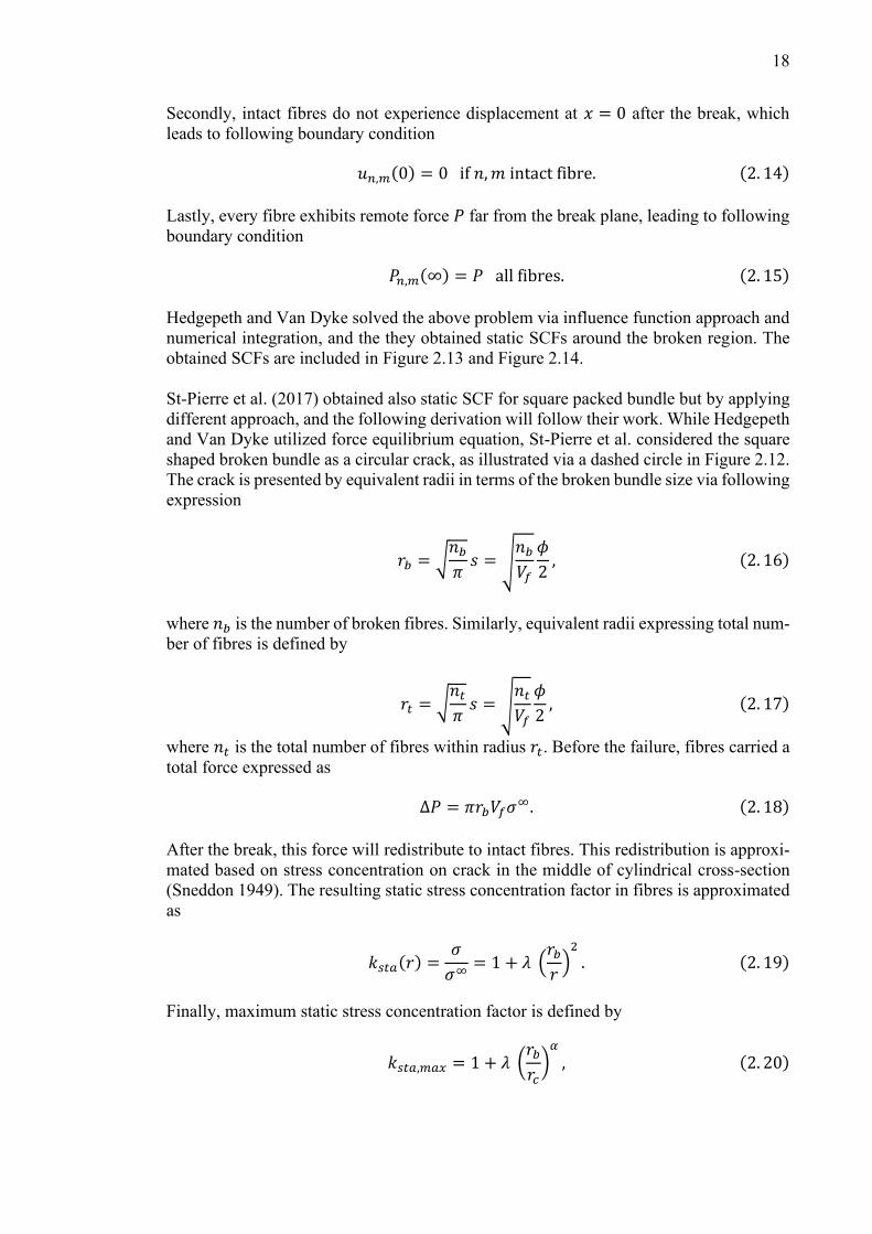
the bundle and the number of broken fibres is odd. Figure 2.13 shows static stress con-

centration factor with respect to distance 𝑟 by different number of broken fibres varying

from 1 to 9. In this example case, volume fraction 𝑉𝑓 has a value of 0.6 and the bundle is

considered large with a total number of 900 fibres. Results show that highest static stress

concentration locates in the fibre that is closest to the centre of broken bundle and quickly

decreases when moving away from the broken region.

Figure 2.13. Analytical static stress concentration factor in fibres with respect the dis-

tance from the centre of broken bundle in 2D square packing (Adapted from St-Pierre et

al. 2017 and Hedgepeth and Van Dyke 1967).

Figure 2.13 also compares maximum SCFs, marked as circles, obtained both by St-Pierre,

Hedgepeth and co-workers. Maximum SCFs were located in both cases in the intact fibre

closest to centre of the broken region. However, the SCFs predicted by Hedgepeth and

Van Dyke are significantly higher than the model of St-Pierre et al. For example, for one

broken fibre the relative difference in SCFs is 10%. This difference can be explained by

the differences in the derivation of models. Hedgepeth and Van Dyke utilized force equi-

librium contributed by matrix shearing and fibre normal force, and corresponding linear

20

elastic constitutive equations. St-Pierre et al. used a fracture mechanics approach by mod-

elling the bundle as a crack and by approximating the stress concentration near the crack

tip. Then they adjusted the model parameters based on the results of their FE simulation.

Even though their expression on static SCF (2.20) did not consider matrix plasticity, the

FE simulation, used for determination of parameters 𝛼 and 𝜆, incorporated perfectly plas-

tic behaviour in matrix.

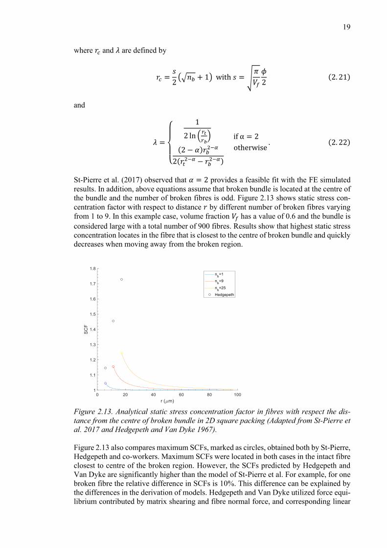
Analytical expressions have been obtained also for hexagonal packed models. Hedgepeth

and van Dyke (1967) obtained an analytical approach to determine static SCFs around

broken fibre in hexagonal packing. Hexagonal packing differs essentially from square

packing in a such way that the number of intact fibres surrounding broken region is dif-

ferent, as seen in Figure 2.13 and Figure 2.14. For example, for one broken fibre hexag-

onal packed bundle has six neighbouring intact fibres in a distance of 𝑑 whereas square

packed bundle has only four intact fibres within this distance.

Figure 2.14. Hexagonally packed composite. (Adapted from Hedgepeth and Van Dyke

1967)

By using expressions (2.10) and (2.11), Hedgepeth and Van Dyke obtained following

expression for equilibrium equation for hexagonal packed composite

𝐸𝐴𝜕2𝑢𝑛,𝑚𝜕𝑥2

+ 𝐺ℎ(𝑢𝑛+1,𝑚 + 𝑢𝑛,𝑚+1 + 𝑢𝑚−1,𝑚 + 𝑢𝑛,𝑚−1 + 𝑢𝑛+1,𝑚−1

+𝑢𝑛−1,𝑚+1 − 6𝑢𝑛,𝑚) = 0. (2. 23)

Fibres labelled by increasing subscript 𝑚 are inclined by 60 degrees with respect to fibres

labelled by increasing subscript 𝑛, as seen in Figure 2.14. Hedgepeth and Van Dyke

solved the equilibrium equation via influence function approach and numerical integra-

tion, and they obtained static SCFs around the broken region. The broken regions are

arranged in hexagonal shape, illustrated in Figure 2.14, and the number of broken fibres

have values 1, 7, 19 etc. Figure 2.14 shows static SCFs for different sizes of broken re-

gions for two locations: i) the intact fibre closest to the centre of broken region ii) the

intact fibre farthest from the centre but in the neighbourhood of the broken region. For

example, for seven broken fibres the closest intact fibre locates at point 𝑐 and farthest

intact fibre at point 𝑏 (see Figure 2.14).

a

b c

d e

𝑛𝑏 = 1

𝑛𝑏 = 7

𝑛𝑏 = 19

21

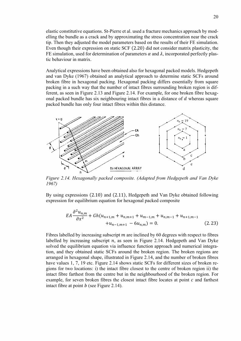
Figure 2.15. Static SCF in hexagonally and square packed composite for different number

of broken fibres. (Adapted from Hedgepeth and Van Dyke 1967)

In hexagonal packed model, static SCF appear to depend significantly on which intact

fibre neighbouring the broken section was examined. For example, SCF varies from 1.25

to 1.41 for only seven broken fibre. On the other hand, SCF seems to be not very sensitive

to the packing type. Comparing square and hexagonal packing for the closest intact fibres,

SCF curves lie rather close to each other. For one broken fibre, the relative difference in

SCF is most significant (5%) due to different number of closest neighbours, but for large

broken regions, i.e. 𝑛𝑏 > 35, the relative difference is under 2%.

2.2.2 Static SCF including matrix plasticity

Previous analytical expressions on static SCF assumed that matrix behaves in linear-elas-

tic manner without a yield limit. In reality, matrix may experience significant shear strains

near the broken region, leading to unrealistically high shear stresses if no plasticity is

included as conducted by quasi-static simulations (Lane et al. 2001). Moreover, the con-

flicting results of Hedgepeth and Van Dyke (1967) and St-Pierre et al. (2017) encourages

to assess the effect of plasticity (see Figure 2.13). Thus, plasticity in model could possibly

obtain important contribution to static SCF. This sub-section obtains an analytical static

model including plasticity only for 1D regular packing since 2D packed analytical plastic

models require laborious mathematical treatment. This section will follow the work by

Hedgepeth and Van Dyke (1967).

Figure 2.16a shows the configuration of analytical model including matrix plasticity. The

model consists of one broken fibre and infinite number of intact fibres. Plasticity is im-

plemented via two steps. First, whole composite is considered to behave by linear elastic

manner in which fibres are assumed to extend along the length, and matrix is assumed to

exhibit only shear deformation. Then, a region of plasticity, determined by parameters 𝑎

and 𝑑, is placed in the region surrounding the break. In this region, the shear stress can

increase linearly until to yield limit value 𝜏 = τy, corresponding perfectly plastic material

model. Shear stress is assumed to be constant at regions between neighbouring fibres

when 𝑥 is held constant.

22

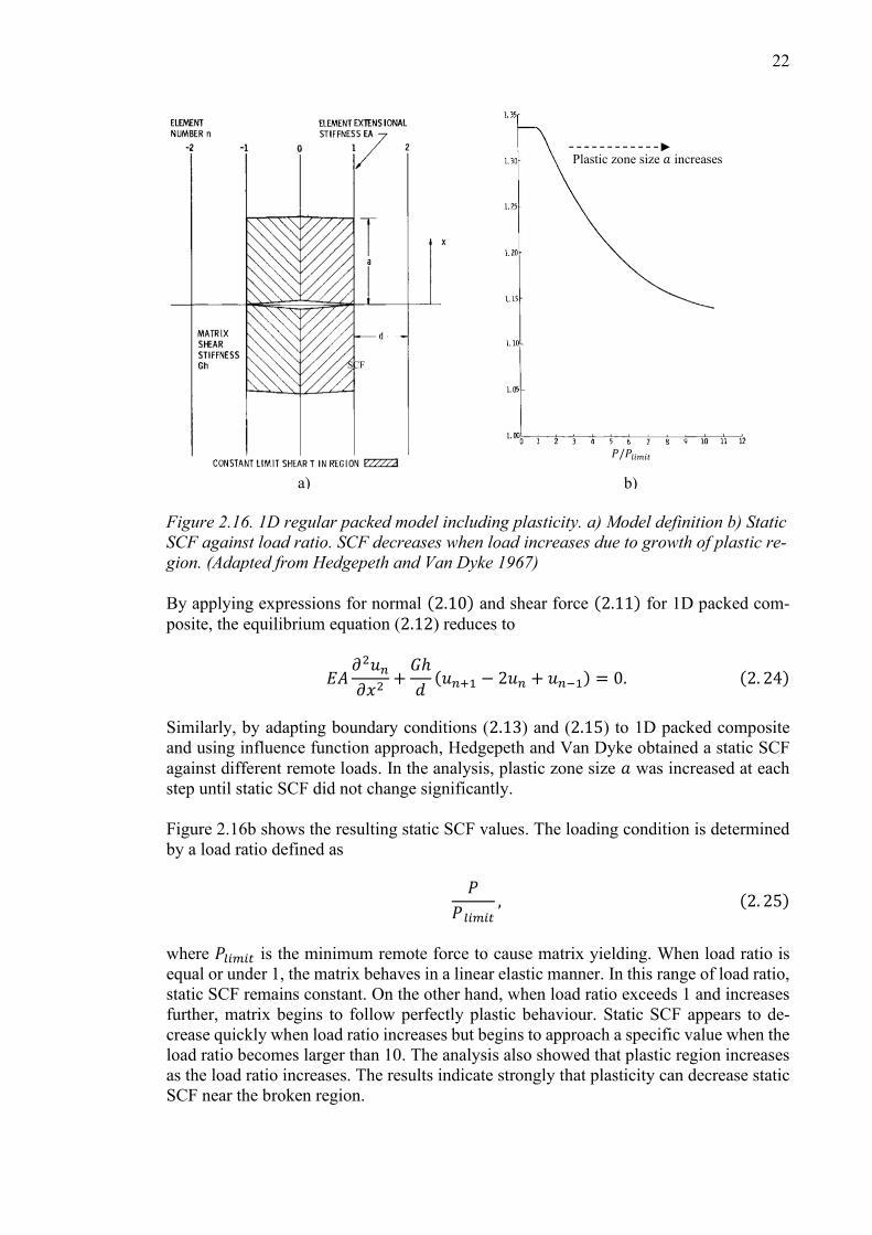
Figure 2.16. 1D regular packed model including plasticity. a) Model definition b) Static

SCF against load ratio. SCF decreases when load increases due to growth of plastic re-

gion. (Adapted from Hedgepeth and Van Dyke 1967)

By applying expressions for normal (2.10) and shear force (2.11) for 1D packed com-

posite, the equilibrium equation (2.12) reduces to

𝐸𝐴𝜕2𝑢𝑛𝜕𝑥2

+𝐺ℎ

𝑑(𝑢𝑛+1 − 2𝑢𝑛 + 𝑢𝑛−1) = 0. (2. 24)

Similarly, by adapting boundary conditions (2.13) and (2.15) to 1D packed composite

and using influence function approach, Hedgepeth and Van Dyke obtained a static SCF

against different remote loads. In the analysis, plastic zone size 𝑎 was increased at each

step until static SCF did not change significantly.

Figure 2.16b shows the resulting static SCF values. The loading condition is determined

by a load ratio defined as

𝑃

𝑃 𝑙𝑖𝑚𝑖𝑡, (2. 25)

where 𝑃𝑙𝑖𝑚𝑖𝑡 is the minimum remote force to cause matrix yielding. When load ratio is

equal or under 1, the matrix behaves in a linear elastic manner. In this range of load ratio,

static SCF remains constant. On the other hand, when load ratio exceeds 1 and increases

further, matrix begins to follow perfectly plastic behaviour. Static SCF appears to de-

crease quickly when load ratio increases but begins to approach a specific value when the

load ratio becomes larger than 10. The analysis also showed that plastic region increases

as the load ratio increases. The results indicate strongly that plasticity can decrease static

SCF near the broken region.

𝑃/𝑃𝑙𝑖𝑚𝑖𝑡

SCF

Plastic zone size 𝑎 increases

a) b)

23

2.2.3 Static stress redistribution along the fibre

To understand deeper the stress distribution within the composite, stresses are studied

more closely along the broken and neighbouring intact fibre. The stress distribution along

the intact fibre defines the probability of failure in different portions of fibre, as described

in section 2.1.4. Illustration is done with one broken fibre with matrix crack between the

intact and broken fibre, as seen in Figure 2.17a. Figure 2.17b illustrates the simulated

stress distribution within the length in both fibres. As Figure 2.18b shows, broken fibre

has zero normal stress at 𝑥 = 0, which increases when moving apart from the fibre break

plane. On the other hand, intact fibre has highest stress at 𝑥 = 0, which decreases even

below the remote stress level, as shown also by Swolfs et al. (2015). Eventually, stresses

in both fibres approach the remote stress 𝜎∞ when distance is sufficiently large, ending

up to a stress state of intact composite.

a) b)

Figure 2.17 a) Illustration of broken fibre, adjacent intact fibre and matrix shearing b)

Simulated SCF in broken and adjacent fibre with respect to relative distance along the

length of fibre (Square 2D packing) (Reproduced from St-Pierre et al. 2017)

The difference of stresses between intact and broken fibre is compensated by the shearing

of matrix. While in intact stage matrix experiences very low stresses, at broken stage

matrix must guarantee the adhesion between fibres that have a stress difference of mag-

nitude of 𝜎∞. This indicates that shear stresses in matrix become more significant near

the break and vanishes when moving apart from the break. The distance in which stresses

recover to intact stage stresses is called recovery length and it is defined by (Pimenta and

Pinho 2013)

𝑙𝑒 =𝑛𝑏𝜋𝜙

2𝜎∞4𝐶𝜏𝑦

with 𝐶 = 2𝜙√𝜋𝑛𝑏𝑉𝑓

, (2. 26)

where 𝜏𝑦 is the shear strength of matrix. 𝐶 denotes the shear lag perimeter, seen in Figure

2.17. Equation (2.26) is applicable for model with linear-elastic perfectly plastic matrix,

and can be used to approximate the minimum length of the numerical model. In addition,

it shows that recovery length when the number of broken fibres increase, i.e. 𝑙𝑒 is propor-

tional to √𝑛𝑏.

Broken fibre

Intact fibre

24

2.2.4 Static SCF via finite element modelling

Models in chapters 2.2.1 and 2.2.2 were based on laborious analytical approaches with

numerical integration schemes. Moreover, they had several limitations. Firstly, they were

not able to incorporate 2D random packing. Secondly, models with plastic matrix were

available only for simple 1D regular packed bundle. Thirdly, the models assumed that the

stress is uniform thorough the cross-section of fibre, i.e. the fibres were considered as a

1-dimensional line elements. A common method to enhance these limited setups is finite

element (FE) modelling. This section reviews the FE analysis results based on literature.

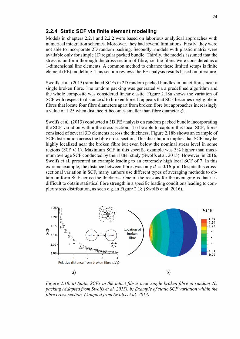
Swolfs et al. (2015) simulated SCFs in 2D random packed bundles in intact fibres near a

single broken fibre. The random packing was generated via a predefined algorithm and

the whole composite was considered linear elastic. Figure 2.18a shows the variation of

SCF with respect to distance 𝑑 to broken fibre. It appears that SCF becomes negligible in

fibres that locate four fibre diameters apart from broken fibre but approaches increasingly

a value of 1.25 when distance 𝑑 becomes smaller than fibre diameter 𝜙.

Swolfs et al. (2013) conducted a 3D FE analysis on random packed bundle incorporating

the SCF variation within the cross section. To be able to capture this local SCF, fibres

consisted of several 3D elements across the thickness. Figure 2.18b shows an example of

SCF distribution across the fibre cross-section. This distribution implies that SCF may be

highly localized near the broken fibre but even below the nominal stress level in some

regions (SCF < 1). Maximum SCF in this specific example was 3% higher than maxi-

mum average SCF conducted by their latter study (Swolfs et al. 2015). However, in 2016,

Swolfs et al. presented an example leading to an extremely high local SCF of 7. In this

extreme example, the distance between fibres was only 𝑑 = 0.15 μm. Despite this cross-

sectional variation in SCF, many authors use different types of averaging methods to ob-

tain uniform SCF across the thickness. One of the reasons for the averaging is that it is

difficult to obtain statistical fibre strength in a specific loading conditions leading to com-

plex stress distribution, as seen e.g. in Figure 2.18 (Swolfs et al. 2016).

a) b)

Figure 2.18. a) Static SCFs in the intact fibres near single broken fibre in random 2D

packing (Adapted from Swolfs et al. 2015). b) Example of static SCF variation within the

fibre cross-section. (Adapted from Swolfs et al. 2013)

𝑑/𝜙

25

As mentioned in chapter 2.2.1, St-Pierre et al. (2017) performed a FE simulation with 2D

square packed composite incorporating linear elastic perfectly plastic matrix. They found

that for one broken fibre, plasticity reduces SCF in relative terms 7% compared to linear

elastic model by Hedgepeth and Van Dyke (1967). For larger bundles this reduction be-

comes more significant, e.g. over 30% for a bundle of 36 broken fibres.

2.3 Dynamic analysis of broken UD composite

Chapter 2.2 considered static stress distribution in composite after the break. However,

during the fibre break, composite will exhibit dynamic behaviour when transforming from

the intact stage to broken stage. This dynamic behaviour can be intuitively described as

an oscillation of the structure settling to a certain deformed shape. This oscillation causes

time-dependent stress distribution and an increase in the maximum stress compared to

settled static composite. The dynamic effects are generally accepted, but analysis has been

proven to be complicated (Hedgepeth 1961, Ji et al. 1985, Sakharova and Ovchinskii

1979, 1980, 1984, Swolfs et al. 2016). Therefore, analytical expressions for dynamic be-

haviour are obtained for simple 1D regular packed composite.

The first subsection illustrates how dynamic stresses initiate and propagate in composite

after the break. The second subsection obtains an analytical expression for the maximum

dynamic SCFs for 1D packed linear elastic model and compares the results to correspond-

ing static SCFs. Third subsection extends from the second subsection but determines the

SCF along the fibre. Final section presents a numerical approach to obtain dynamic

stresses via finite element modelling.

2.3.1 Dynamic stress propagation

To understand dynamics of a composite consisting two distinct phases of materials, one

could first examine the dynamics of these two components separately. This section will

follow the work by Meyers (1994) and is presented in the context of fibre reinforced

composites.

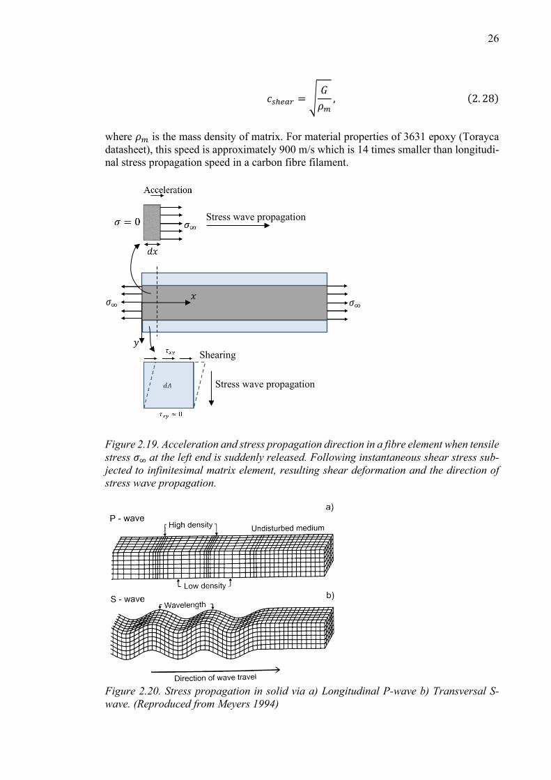
Stresses can propagate in solid via two fundamental mechanisms: via tensile and shear

stresses. Tensile stress propagation can be illustrated by considering a bar or fibre element

seen in Figure 2.24a. If a bar element is initially loaded in tension and the other end is

suddenly released, the bar compensates this imbalance by transferring the stresses to the

other end causing a local acceleration. This results to a longitudinal stress wave, or P-

wave, propagation in material. P-wave propagation causes a time dependent variation in

density and stresses in solid as seen in Figure 2.20a. This longitudinal stress wave prop-

agation speed can be expressed as

𝑐𝐿 = √𝐸𝑓

𝜌𝑓, (2. 27)

where 𝜌𝑓 is the mass density of the fibre. Again, for material properties of carbon fibre

filament T800H (St-Pierre et al. 2017), this propagation speed is over 12000 m/s. On the

other hand, an accelerating fibre element causes sudden shear stresses in matrix material

illustrated in Figure 2.19. These shear stresses propagate transversely in matrix material

resulting in S-wave propagation seen in Figure 2.20b. Similar to P-wave, S-wave propa-

gation speed is closely related to material properties via following relation

26

𝑐𝑠ℎ𝑒𝑎𝑟 = √𝐺

𝜌𝑚, (2. 28)

where 𝜌𝑚 is the mass density of matrix. For material properties of 3631 epoxy (Torayca

datasheet), this speed is approximately 900 m/s which is 14 times smaller than longitudi-

nal stress propagation speed in a carbon fibre filament.

Figure 2.19. Acceleration and stress propagation direction in a fibre element when tensile

stress 𝜎∞ at the left end is suddenly released. Following instantaneous shear stress sub-

jected to infinitesimal matrix element, resulting shear deformation and the direction of

stress wave propagation.

Figure 2.20. Stress propagation in solid via a) Longitudinal P-wave b) Transversal S-

wave. (Reproduced from Meyers 1994)

Stress wave propagation

Stress wave propagation

Shearing

𝑥

𝑦

27

Besides these two fundamental mechanisms, stress waves can propagate by combining

these propagation types. One of these combined propagation types is Rayleigh wave

which travels especially along the free surfaces of the structure. In addition, stress waves

may reflect from the boundaries of the model on when encountering an interface of dif-

ferent material.

2.3.2 Dynamic stress concentration factor

This section presents the analytical expressions for dynamic stresses in fibre break plane

in 1D packed composite. The content will follow the work by Hedgepeth (1961) if not

mentioned otherwise. In addition, the end of the section reviews a 2D packed analytical

model by Sakharova and Ovchinskii (1980).

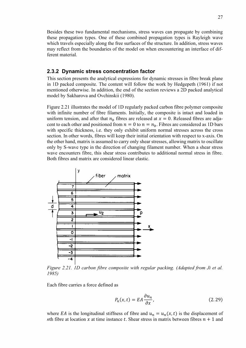
Figure 2.21 illustrates the model of 1D regularly packed carbon fibre polymer composite

with infinite number of fibre filaments. Initially, the composite is intact and loaded in

uniform tension, and after that 𝑛𝑏 fibres are released at 𝑥 = 0. Released fibres are adja-

cent to each other and positioned from 𝑛 = 0 to 𝑛 = 𝑛𝑏. Fibres are considered as 1D bars

with specific thickness, i.e. they only exhibit uniform normal stresses across the cross

section. In other words, fibres will keep their initial orientation with respect to x-axis. On

the other hand, matrix is assumed to carry only shear stresses, allowing matrix to oscillate

only by S-wave type in the direction of changing filament number. When a shear stress

wave encounters fibre, this shear stress contributes to additional normal stress in fibre.

Both fibres and matrix are considered linear elastic.

Figure 2.21. 1D carbon fibre composite with regular packing. (Adapted from Ji et al.

1985)

Each fibre carries a force defined as

𝑃𝑛(𝑥, 𝑡) = 𝐸𝐴𝜕𝑢𝑛𝜕𝑥

, (2. 29)

where 𝐸𝐴 is the longitudinal stiffness of fibre and 𝑢𝑛 = 𝑢𝑛(𝑥, 𝑡) is the displacement of

nth fibre at location 𝑥 at time instance 𝑡. Shear stress in matrix between fibres 𝑛 + 1 and

28

𝑛 𝑆𝑛+1,𝑛 is assumed uniform across the distance 𝑑 and can be defined via displacements

of these fibres by

𝑆𝑛+1,𝑛 = 𝐺ℎ(𝑢𝑛+1 − 𝑢𝑛)

𝑑. (2. 30)

where 𝐺ℎ is the shear stiffness of matrix. Hence, equation of motion for 𝑛th filament can

be expressed as

𝐸𝐴𝜕2𝑢𝑛𝜕𝑥2

+𝐺ℎ

𝑑(𝑢𝑛+1 − 2𝑢𝑛 + 𝑢𝑛−1) = 𝑚𝑙

𝜕2𝑢𝑛𝜕𝑡2

, (2. 31)

where 𝑚𝑙 denotes mass per unit length. Here it is assumed that 𝑚𝑙 is concentrated at the

corresponding filament. Since 𝑛𝑏 broken filaments are released at the beginning of the

analysis, i.e. at 𝑡 = 0, following boundary conditions hold for displacements and forces

at the fibre break plane

𝑢𝑛(0, 𝑡) = 0 when 𝑛 < 0 or 𝑛 ≥ 𝑛𝑏 (2. 32)and

𝑃𝑛(0, 𝑡) = 0 when 0 ≤ 𝑛 ≤ 𝑛𝑏 − 1. (2. 33)

Since uniform remote loading, denoting as 𝑃, is applied at 𝑥 → ∞, following boundary

condition holds for each fibre

𝑃𝑛(±∞, 𝑡) = 𝑃. (2. 34)

Initially all fibres are loaded uniformly with force 𝑃 thorough their length. In addition, it

is assumed that fibres are in rest at the beginning of analysis. This leads to following

initial conditions

𝑃𝑛(𝑥, 0) = 𝑃 (2. 35)

and

𝜕𝑢𝑛𝜕𝑡

(𝑥, 0) = 0. (2. 36)

Hedgepeth was not able to find a closed form solution for this problem. Instead, he dis-

covered that dynamic stress concentration factor 𝑘𝑑𝑦𝑛 has a complicated implicit form of

𝑘𝑑𝑦𝑛(𝑡∗) =1

2𝜋𝑖∮ 𝑘𝑑𝑦𝑛

∗ (𝑠∗)𝑒𝑠𝑡∗𝑑𝑠∗

𝐶∗

, (2. 37)

where 𝑡∗ is dimensionless time, 𝑠∗ is a Laplace transform variable, 𝑘𝑑𝑦𝑛∗ (𝑠∗) is a Laplace

transform of dynamic stress concentration factor, 𝐶∗ is a closed loop around the broken

region and 𝑖 is a imaginary unit. He did however a numerical evaluation via power series

and obtained approximation for dynamic behaviour. He also confirmed that highest

stresses occur at fibre break plane in intact fibres closest to the broken fibre region.

29

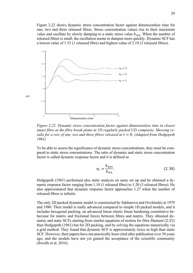
Figure 2.22 shows dynamic stress concentration factor against dimensionless time for

one, two and three released fibres. Stress concentration values rise to their maximum

value and oscillate by slowly damping to a static stress value 𝑘𝑠𝑡𝑎. When the number of

released fibres is small, the oscillation seems to dampen more quickly. Dynamic SCF has

a lowest value of 1.53 (1 released fibre) and highest value of 2.19 (3 released fibres).

Figure 2.22. Dynamic stress concentration factor against dimensionless time in closest

intact fibre at the fibre break plane in 1D regularly packed UD composite. Showing re-

sults for a row of one, two and three fibres released at 𝑡 = 0. (Adapted from Hedgepeth

1961)

To be able to assess the significance of dynamic stress concentrations, they must be com-

pared to static stress concentrations. The ratio of dynamic and static stress concentration

factor is called dynamic response factor and it is defined as

𝜂𝑟 =𝑘𝑑𝑦𝑛

𝑘𝑠𝑡𝑎. (2. 38)

Hedgepeth (1961) performed also static analysis on same set up and he obtained a dy-

namic response factor ranging from 1.10 (1 released fibre) to 1.20 (3 released fibres). He

also approximated that dynamic response factor approaches 1.27 when the number of

released fibres is infinite.

The only 2D packed dynamic model is constructed by Sakharova and Ovchinskii at 1979

and 1980. Their model is really advanced compared to simple 1D packed models, and it

includes hexagonal packing, an advanced linear elastic linear hardening constitutive be-

haviour for matrix and frictional forces between fibres and matrix. They obtained dy-

namic and static SCFs starting from similar equations of motion for fibre filament (2.31) than Hedgepeth (1961) but for 2D packing, and by solving the equations numerically via

a grid method. They found that dynamic SCF is approximately twice as high than static

SCF. However, their papers have not practically been cited after publication over 30 years

ago, and the models have not yet gained the acceptance of the scientific community

(Swolfs et al. 2016).

𝑛𝑏 = 1

𝑛𝑏 = 2

𝑛𝑏 = 3

SCF

Dimensionless time

30

2.3.3 Dynamic SCF along the intact fibre

As Hedgepeth (1961) concluded, dynamic SCFs may be significant in the intact fibres

near the broken region at the fibre break plane. However, to be able to explain co-planarity

of the fibre breaks, SCFs must be studied along the intact fibre. Co-planar break occur-

rence would at least require that dynamic stresses are significant over a length corre-

sponding the fibre diameter but along longitudinal direction of the intact fibre. Ji et al.

(1985) determined dynamic SCF variation along the fibre length in the intact fibre, and

this section will follow their work.

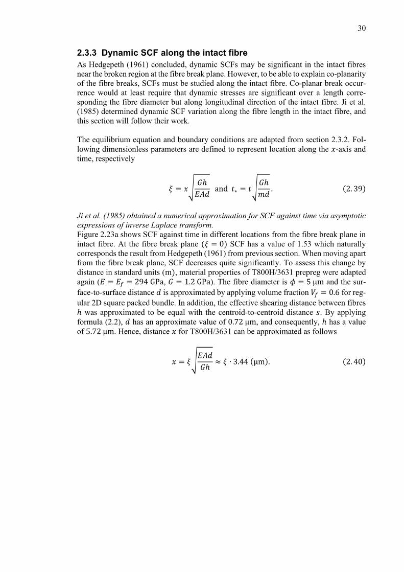
The equilibrium equation and boundary conditions are adapted from section 2.3.2. Fol-

lowing dimensionless parameters are defined to represent location along the 𝑥-axis and

time, respectively

𝜉 = 𝑥√𝐺ℎ

𝐸𝐴𝑑 and 𝑡∗ = 𝑡√

𝐺ℎ

𝑚𝑑. (2. 39)

Ji et al. (1985) obtained a numerical approximation for SCF against time via asymptotic

expressions of inverse Laplace transform.

Figure 2.23a shows SCF against time in different locations from the fibre break plane in

intact fibre. At the fibre break plane (𝜉 = 0) SCF has a value of 1.53 which naturally

corresponds the result from Hedgepeth (1961) from previous section. When moving apart

from the fibre break plane, SCF decreases quite significantly. To assess this change by

distance in standard units (m), material properties of T800H/3631 prepreg were adapted

again (𝐸 = 𝐸𝑓 = 294 GPa, 𝐺 = 1.2 GPa). The fibre diameter is 𝜙 = 5 μm and the sur-

face-to-surface distance 𝑑 is approximated by applying volume fraction 𝑉𝑓 = 0.6 for reg-

ular 2D square packed bundle. In addition, the effective shearing distance between fibres

ℎ was approximated to be equal with the centroid-to-centroid distance 𝑠. By applying

formula (2.2), 𝑑 has an approximate value of 0.72 μm, and consequently, ℎ has a value

of 5.72 μm. Hence, distance 𝑥 for T800H/3631 can be approximated as follows

𝑥 = 𝜉√𝐸𝐴𝑑

𝐺ℎ≈ 𝜉 ∙ 3.44 (μm). (2. 40)

31

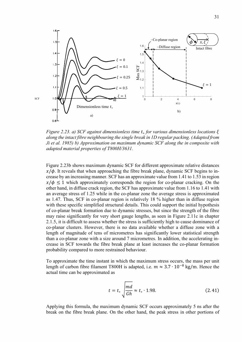
Figure 2.23. a) SCF against dimensionless time 𝑡∗ for various dimensionless locations 𝜉

along the intact fibre neighbouring the single break in 1D regular packing. (Adapted from

Ji et al. 1985) b) Approximation on maximum dynamic SCF along the in composite with

adapted material properties of T800H/3631.

Figure 2.23b shows maximum dynamic SCF for different approximate relative distances

𝑥/𝜙. It reveals that when approaching the fibre break plane, dynamic SCF begins to in-

crease by an increasing manner. SCF has an approximate value from 1.41 to 1.53 in region

𝑥/𝜙 ≤ 1 which approximately corresponds the region for co-planar cracking. On the

other hand, in diffuse crack region, the SCF has approximate value from 1.16 to 1.41 with

an average stress of 1.25 while in the co-planar zone the average stress is approximated

as 1.47. Thus, SCF in co-planar region is relatively 18 % higher than in diffuse region

with these specific simplified structural details. This could support the initial hypothesis

of co-planar break formation due to dynamic stresses, but since the strength of the fibre

may raise significantly for very short gauge lengths, as seen in Figure 2.11c in chapter

2.1.5, it is difficult to assess whether the stress is sufficiently high to cause dominance of

co-planar clusters. However, there is no data available whether a diffuse zone with a

length of magnitude of tens of micrometres has significantly lower statistical strength

than a co-planar zone with a size around 7 micrometres. In addition, the accelerating in-

crease in SCF towards the fibre break plane at least increases the co-planar formation

probability compared to more restrained behaviour.

To approximate the time instant in which the maximum stress occurs, the mass per unit

length of carbon fibre filament T800H is adapted, i.e. 𝑚 ≈ 3.7 ∙ 10−8 kg/m. Hence the

actual time can be approximated as

𝑡 = 𝑡∗ √𝑚𝑑

𝐺ℎ≈ 𝑡∗ ∙ 1.98. (2. 41)

Applying this formula, the maximum dynamic SCF occurs approximately 5 ns after the

break on the fibre break plane. On the other hand, the peak stress in other portions of

~Co-planar region

~Diffuse region Intact fibre

Dimensionless time 𝑡∗

𝜉 = 0

𝜉 = 0.1

𝜉 = 0.25

𝜉 = 0.5

𝜉 = 1

𝜉 = 1

SCF

a) b)

32

intact fibre occurs slightly later. For example, at point 𝑥 = 7 ∙ 𝜙 which is beyond the

cluster zone, the maximum stress occurs 7 ns after break.

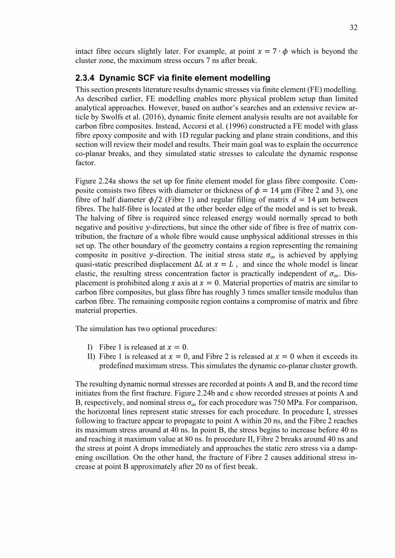
2.3.4 Dynamic SCF via finite element modelling

This section presents literature results dynamic stresses via finite element (FE) modelling.

As described earlier, FE modelling enables more physical problem setup than limited

analytical approaches. However, based on author’s searches and an extensive review ar-

ticle by Swolfs et al. (2016), dynamic finite element analysis results are not available for

carbon fibre composites. Instead, Accorsi et al. (1996) constructed a FE model with glass

fibre epoxy composite and with 1D regular packing and plane strain conditions, and this

section will review their model and results. Their main goal was to explain the occurrence

co-planar breaks, and they simulated static stresses to calculate the dynamic response

factor.

Figure 2.24a shows the set up for finite element model for glass fibre composite. Com-

posite consists two fibres with diameter or thickness of 𝜙 = 14 μm (Fibre 2 and 3), one

fibre of half diameter 𝜙/2 (Fibre 1) and regular filling of matrix 𝑑 = 14 μm between

fibres. The half-fibre is located at the other border edge of the model and is set to break.

The halving of fibre is required since released energy would normally spread to both

negative and positive 𝑦-directions, but since the other side of fibre is free of matrix con-

tribution, the fracture of a whole fibre would cause unphysical additional stresses in this

set up. The other boundary of the geometry contains a region representing the remaining

composite in positive 𝑦-direction. The initial stress state 𝜎∞ is achieved by applying

quasi-static prescribed displacement Δ𝐿 at 𝑥 = 𝐿 , and since the whole model is linear

elastic, the resulting stress concentration factor is practically independent of 𝜎∞. Dis-

placement is prohibited along 𝑥 axis at 𝑥 = 0. Material properties of matrix are similar to

carbon fibre composites, but glass fibre has roughly 3 times smaller tensile modulus than

carbon fibre. The remaining composite region contains a compromise of matrix and fibre

material properties.

The simulation has two optional procedures:

I) Fibre 1 is released at 𝑥 = 0.

II) Fibre 1 is released at 𝑥 = 0, and Fibre 2 is released at 𝑥 = 0 when it exceeds its

predefined maximum stress. This simulates the dynamic co-planar cluster growth.

The resulting dynamic normal stresses are recorded at points A and B, and the record time

initiates from the first fracture. Figure 2.24b and c show recorded stresses at points A and

B, respectively, and nominal stress 𝜎∞ for each procedure was 750 MPa. For comparison,

the horizontal lines represent static stresses for each procedure. In procedure I, stresses

following to fracture appear to propagate to point A within 20 ns, and the Fibre 2 reaches

its maximum stress around at 40 ns. In point B, the stress begins to increase before 40 ns

and reaching it maximum value at 80 ns. In procedure II, Fibre 2 breaks around 40 ns and

the stress at point A drops immediately and approaches the static zero stress via a damp-

ening oscillation. On the other hand, the fracture of Fibre 2 causes additional stress in-

crease at point B approximately after 20 ns of first break.

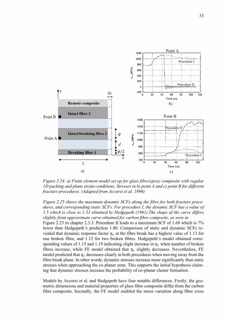
33

Figure 2.24. a) Finite element model set up for glass fibre/epoxy composite with regular

1D packing and plane strain conditions. Stresses in b) point A and c) point B for different

fracture procedures. (Adapted from Accorsi et al. 1996)

Figure 2.25 shows the maximum dynamic SCFs along the fibre for both fracture proce-

dures, and corresponding static SCFs. For procedure I, the dynamic SCF has a value of

1.5 which is close to 1.53 obtained by Hedgepeth (1961).The shape of the curve differs

slightly from approximate curve obtained for carbon fibre composite, as seen in

Figure 2.23 in chapter 2.3.3. Procedure II leads to a maximum SCF of 1.68 which is 7%

lower than Hedgepeth’s prediction 1.80. Comparison of static and dynamic SCFs re-

vealed that dynamic response factor 𝜂𝑟 at the fibre break has a highest value of 1.13 for

one broken fibre, and 1.12 for two broken fibres. Hedgepeth’s model obtained corre-

sponding values of 1.15 and 1.19 indicating slight increase in 𝜂𝑟 when number of broken

fibres increase, while FE model obtained that 𝜂𝑟 slightly decreases. Nevertheless, FE

model predicted that 𝜂𝑟 decreases clearly in both procedures when moving away from the

fibre break plane. In other words, dynamic stresses increase more significantly than static

stresses when approaching the co-planar zone. This supports the initial hypothesis claim-

ing that dynamic stresses increase the probability of co-planar cluster formation.

Models by Accorsi et al. and Hedgepeth have four notable differences. Firstly, the geo-

metric dimensions and material properties of glass fibre composite differ from the carbon

fibre composite. Secondly, the FE model enabled the stress variation along fibre cross

Point A

Point B

Procedure I

Procedure II

Procedure I

Procedure II

a)

b)

c)

34

section while previous models assumed that the stress is uniform. In FE model, stresses

were recorded close to the surface of fibre instead of the centreline of fibre. Thirdly,

Hedgepeth’s model assumed that resin between fibres is modelled by one shear spring

element and fibres as one-dimensional longitudinal springs. The FE model naturally con-

tains significantly larger number of elements and allows more versatile forms of mechan-

ical behaviour. For example, the FE model allows matrix elements to exhibit not only

shear stresses but also normal stresses, and fibres are also allowed to carry bending mo-

ments and oscillate transversely (see Figure 2.20b). Lastly, procedure II assumed that the

second fibre is released after some time period after the break while Hedgepeth assumed

that breaks occur simultaneously.

Figure 2.25. Dynamic and static SCFs along the fibre for a) procedure I at point A (Fibre

2 breaks) and b) procedure II at point B (Fibre 2 breaks and Fibre 3 breaks subsequently).

2.4 SCF summary

In this thesis, stress concentration factor (SCF) is the key tool in explaining the mechan-

ical behaviour and fracture probability. This chapter summarizes the static and dynamic

SCFs retrieved via a literature review. Table 2.1 compiles these SCFs for different anal-

ysis setups, and the results are obtained either analytically or numerically via FEM. SCFs

here are obtained for the nearest intact fibre at the fibre break plane, and for only one

broken fibre. The results emphasize static SCFs since there are only a few dynamic mod-

els in the literature.

The comparison of literature results on static models reveals four main trends. Firstly,

static SCFs are evidently larger for 1D packed models than 2D packed models. In relative

terms this increase is up 17 % when comparing regular 1D packed and regular 2D models.

Secondly, static SCF decrease when incorporating plastic matrix. This decrease is from 3

to 15 % depending on the packing type, matrix material model and applied load. Thirdly,

FE simulation results differ slightly from corresponding analytical results. For hexagonal

and square packed models with linear elastic matrix this difference is up to 7 %. For 1D

regular packed model this difference was over 11%. Therefore, one could deduce that

analytical models appear not to capture precisely all the relevant physical mechanisms for

static analysis. Lastly, static SCFs can be clearly larger when applying random packing

of distorted geometry. The static SCFs for random packing had values up to 1.25 (Swolfs

et al. 2015) which is over 14 % higher than in square or hexagonal packed model. Even

higher static SCFs were captured in distorted square packed geometry in which one fibre

was manually relocated (Landis and McMeeking 1999), resulting in a maximum static

SCF of 1.41.

Co-planar Co-planar Diffuse Diffuse

dynamic dynamic

static static

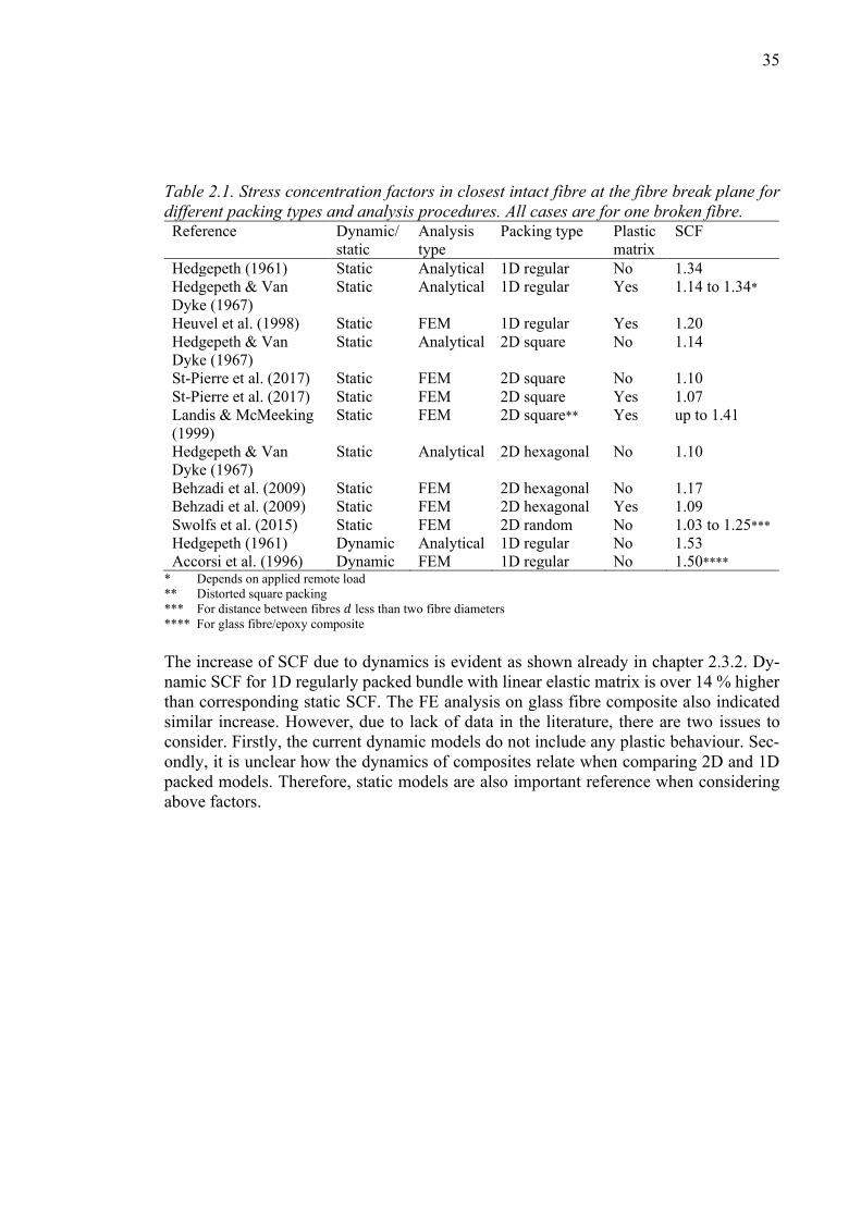
35

Table 2.1. Stress concentration factors in closest intact fibre at the fibre break plane for

different packing types and analysis procedures. All cases are for one broken fibre. Reference Dynamic/

static

Analysis

type

Packing type Plastic

matrix

SCF

Hedgepeth (1961) Static Analytical 1D regular No 1.34

Hedgepeth & Van

Dyke (1967)

Static Analytical 1D regular Yes 1.14 to 1.34*

Heuvel et al. (1998) Static FEM 1D regular Yes 1.20

Hedgepeth & Van

Dyke (1967)

Static Analytical 2D square No 1.14

St-Pierre et al. (2017) Static FEM 2D square No 1.10

St-Pierre et al. (2017) Static FEM 2D square Yes 1.07

Landis & McMeeking

(1999)

Static FEM 2D square** Yes up to 1.41

Hedgepeth & Van

Dyke (1967)

Static Analytical 2D hexagonal No 1.10

Behzadi et al. (2009) Static FEM 2D hexagonal No 1.17

Behzadi et al. (2009) Static FEM 2D hexagonal Yes 1.09

Swolfs et al. (2015) Static FEM 2D random No 1.03 to 1.25***

Hedgepeth (1961) Dynamic Analytical 1D regular No 1.53

Accorsi et al. (1996) Dynamic FEM 1D regular No 1.50**** ** Depends on applied remote load

** Distorted square packing

*** For distance between fibres 𝑑 less than two fibre diameters

**** For glass fibre/epoxy composite

The increase of SCF due to dynamics is evident as shown already in chapter 2.3.2. Dy-

namic SCF for 1D regularly packed bundle with linear elastic matrix is over 14 % higher

than corresponding static SCF. The FE analysis on glass fibre composite also indicated

similar increase. However, due to lack of data in the literature, there are two issues to

consider. Firstly, the current dynamic models do not include any plastic behaviour. Sec-

ondly, it is unclear how the dynamics of composites relate when comparing 2D and 1D

packed models. Therefore, static models are also important reference when considering

above factors.

36

3 Dynamic finite element model

Since analytical analysis for dynamic breakage is complicated for 2D packed models, a

numerical approach is required. A common numerical method for UD composites is finite

element method (FEM). First section presents in detail the dynamic finite element model

including geometry, meshing, boundary conditions and material models. The dynamic FE

model is extended version of quasi-static model by St-Pierre et al. (2017) with only es-

sential modifications. The FE model uses dynamic explicit solver with default settings in

Abaqus/CAE 2017. Second section presents a systematic calibration and validation pro-

cess which obtains appropriate model parameters.

3.1 Model description

3.1.1 Geometry and mesh

Figure 3.1 shows one variation of the geometry of the finite element model. Model rep-

resents a composite of length 2𝐿 in which breaks are located at the centre plane of the

structure. Since the model utilizes symmetry, the length of the model can be reduced to

𝐿, thus the fibre break plane is located at the border of the model at 𝑥 = 0. Geometry is

modelled by combining rectangular prism shaped unit cells which contain a fibre sur-

rounded by matrix. The dimensions of the unit cell are defined by length of the model 𝐿,

fibre diameter 𝜙 and volume fraction 𝑉𝑓, given as input parameters.

Elements are periodical in the direction of 𝑥-axis which indicates that all element nodes

locate on planes at every 𝐿/𝑛𝐿 increment in x-axis, where 𝑛𝐿 denotes the number of ele-

ments in the longitudinal direction. In addition, 𝑛𝑢 denotes the number of elements at the

border of unit cell and 𝑛𝑟 denotes the number of elements from the fibre perimeter to edge

of unit cell. Element borders start from fibre perimeter propagating in radial direction

ending at the edge of a unit cell. These lines are divided in equal lengths by 𝑛𝑟. The whole

bundle is formed by placing unit cells in square packed form and by merging the nodes

at the outer border of adjacent unit cells. The number of unit cells, i.e. the total number

fibres, is denoted by 𝑛𝑡, and the number of broken fibres is denoted by 𝑛𝑏. The values for

mesh parameters are verified by a calibration process in chapter 3.2.3. The element length

in longitudinal direction 𝑒𝑥 is constant and is defined by

𝑒𝑥 =𝐿

𝑛𝐿. (3.1)

The element dimension in radial direction 𝑒𝑟 lies within bounds defined as

𝜙

2𝑛𝑟(√

𝜋

4𝑉𝑓− 1) ≤ 𝑒𝑟 ≤

𝜙

𝑛𝑟(√

𝜋

2𝑉𝑓− 1) . (3.2)

Third element size, having a maximum value at the edge of unit cell and smallest value

at the fibre perimeter, is defined by

𝑒𝑢 ≤𝜙 + 𝑑

𝑛𝑢=

𝜙

2𝑛𝑢√𝜋

𝑉𝑓. (3.3)

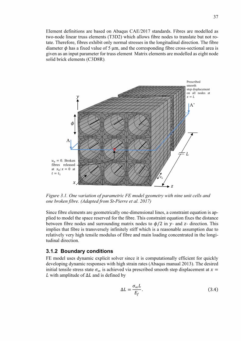
37

Element definitions are based on Abaqus CAE/2017 standards. Fibres are modelled as

two-node linear truss elements (T3D2) which allows fibre nodes to translate but not ro-

tate. Therefore, fibres exhibit only normal stresses in the longitudinal direction. The fibre

diameter 𝜙 has a fixed value of 5 μm, and the corresponding fibre cross-sectional area is

given as an input parameter for truss element Matrix elements are modelled as eight node

solid brick elements (C3D8R).

Figure 3.1. One variation of parametric FE model geometry with nine unit cells and

one broken fibre. (Adapted from St-Pierre et al. 2017)

Since fibre elements are geometrically one-dimensional lines, a constraint equation is ap-

plied to model the space reserved for the fibre. This constraint equation fixes the distance

between fibre nodes and surrounding matrix nodes to 𝜙/2 in 𝑦- and 𝑧- direction. This

implies that fibre is transversely infinitely stiff which is a reasonable assumption due to

relatively very high tensile modulus of fibre and main loading concentrated in the longi-

tudinal direction.

3.1.2 Boundary conditions

FE model uses dynamic explicit solver since it is computationally efficient for quickly

developing dynamic responses with high strain rates (Abaqus manual 2013). The desired

initial tensile stress state 𝜎∞ is achieved via prescribed smooth step displacement at 𝑥 =𝐿 with amplitude of Δ𝐿 and is defined by

Δ𝐿 =𝜎∞𝐿

𝐸𝑓. (3.4)

Prescribed

smooth

step displacement on all nodes at

𝑥 = 𝐿

A’

𝑢𝑥 = 0. Broken

fibres released

at 𝑥0: 𝑥 = 0 at

𝑡 = 𝑡1

𝑧 𝑥

𝑦

𝐿

A

A’

𝜙

𝑒𝐿

38

The displacement occurs within a time period from 0 to 𝑡1, denoting the period of stress

state initiation, i.e. Step 1, as seen in Figure 3.2. Consequently, the aim is to achieve

constant remote stress 𝜎∞ in every fibre before 𝑡 = 𝑡1. After 𝑡1, displacement is kept

constant at 𝑥 = 𝐿. At 𝑡 = 𝑡1, broken fibre nodes at 𝑥 = 0 are released to simulate the

fracture. In case of multiple breaking fibres, all broken fibre nodes are released simulta-

neously. This assumption on simultaneous break is in line with the experiments (Swolfs

et al. 2015) which implied that clusters form at very short time period, as described in

chapter 2.1.3.

The released fibres are arranged either in a square shape (1, 4 and 9 fibres) or in a row

(2,3 and 4 fibres), and the resulting stresses are monitored in the neighbouring intact fi-

bres. Figure 3.4a and b illustrate the arrangement of broken fibres and the neighbouring

stress recording points at 𝑥 = 0. Stresses are monitored for a time period of Δ𝑡 = 𝑡2, and

the highest stress is recorded to obtain dynamic SCF. This monitoring period, i.e. Step 2,

corresponds the period for post-release dynamics. Since displacement is applied at 𝑥 = 𝐿

and stresses are monitored at 𝑥 = 0, there is a small delay from displacement increment

to increase of stress due to finite stress wave propagation speed. The total time of simu-

lation is defined as

𝑡𝑡 = 𝑡1 + 𝑡2. (3.5)

Due to complexity and high number of nodes in the model, the total time must be opti-

mized to enable reasonable computation time. Figure 3.2 illustrates the simulation includ-

ing the prescribed displacement and observed stresses. The maximum stress 𝜎𝑚𝑎𝑥 is com-

pared to nominal stress 𝜎∞, observed at the end of Step 1, to obtain dynamic SCF for each

simulation.

Figure 3.2. Illustration of the simulation. Prescribed displacement at 𝑥 = 𝐿 and resulting

stresses at fibre break plane (𝑥 = 0) against time. A slight delay is expected due to limited

stress wave propagation speed from 𝑥𝐿 to 𝑥0.

Nodes at 𝑥 = 0 have a symmetric boundary condition which does not allow translation

in the direction of 𝑥-axis, as seen in Figure 3.3. This models the actual mechanical be-

haviour of the fibre break plane in a composite of length 2𝐿. The symmetric boundary

condition is naturally released for broken fibres node for Step 2. Another boundary con-

dition is required to restrict the rigid body movement of the whole model in the 𝑦-

𝑧 −plane. Even though, in theory, there are no loads causing this transversal movement,

𝐿

𝑥 = 0

Δ𝐿

39

a stepwise numerical solver might yield transversal forces subjected to the model. This

boundary condition is accomplished by picking a node at the centre of the cross-section

at 𝑥 = 0 and restricting its translation along 𝑦- and 𝑧-axis.

Figure 3.3. View A-A’: Boundary conditions at 𝑥 = 0 and desired stress state before fibre

break. Example for one broken fibre.

The adhesion between matrix and fibre is assumed perfect, i.e. fibres can not slide with

respect to matrix, which is reasonable assumption based on the experimental evidence

carbon fibre epoxy composites, as described in chapter 2.1.3. The constraint is applied to

all fibre nodes except broken nodes to at 𝑥 = 0. This debonding of a broken node results

in the small debonding length, corresponding 𝑒𝐿, in the model which reduces if the ele-

ment size decreases. The small debonding is required to enable dynamic behaviour due

to breakage and its effect on SCF will be negligible, as confirmed later in chapter 3.2.3.

Figure 3.4. Cross-section at 𝑥 = 0: Examples of released nodes and stress recording

points for a) nine broken fibres in square arrangement b) two broken fibres arranged in

a row. Broken fibres are always located at the centre of the bundle to minimize effects of

anti-symmetry.

Released fibres at

𝑡 = 𝑡1

Stresses recorded

𝑦

40

3.1.3 Material modelling

The material properties are defined to represent T800H/3631 carbon fibre epoxy prepreg.

To assess the effect plasticity and constitutive behaviour of matrix, epoxy resin is mod-

elled as i) linear elastic with no limitations on stress ii) linear elastic perfectly plastic with

shear strength 𝜏𝑦. Fibres are modelled as linear elastic with no limit for maximum stress.

Table 3.1 shows the applied material properties. Most material properties are adapted

from St-Pierre et al. (2017). Besides, the density of 3631 epoxy was not directly available

but was approximated via a datasheet provided by the manufacturer (Torayca prepreg

datasheet). All the material parameters are kept constant thorough the simulations.

Table 3.1. Material parameters for dynamic finite element model (T800H/3631).

3.2 Model calibration

Since the parametric finite element model may be occasionally large and detailed with

vast number of elements, the computation time can increase significantly. Therefore, a

systematic model calibration was performed to avoid modification of large number of

parameters and to optimize computation time for primary simulations. In addition, these

calibration simulations attempted to validate the model to prohibit any numerical or phys-

ical distortions during primary simulations. Furthermore, the aim of the calibration sim-

ulations was to discover the actual dynamic behaviour following the breakage. Some of

the parameters, such as bundle size, number of released fibres and material parameters,

were fixed for the calibration simulations, as shown in Table 3.2.

Table 3.2. Fixed parameters for the calibration simulations

Appropriate parameters were selected by monitoring the sensitivity of parameters to max-

imum SCF and by observing the shape of stress versus time curve. Calibration simulations

followed the workflow presented in Figure 3.5. Before the calibration process, some ini-

tial parameter values were selected. First, calibration determined optimal step times 𝑡1

and 𝑡2 by studying dynamic stress propagation and by analysing the stress response with

different parameter values. Secondly, the model length was varied to discover to aid de-

termine the approximate time instant for maximum stress occurrence. Thirdly, the effect

of mesh density was determined by varying the three mesh parameters distinctly. Finally,

all the previous parameters were fixed, and the model was validated by varying the remote

stress 𝜎∞ for both elastic and plastic matrix.

Parameter Value

Fibre tensile modulus 𝐸𝑓 294 GPa

Matrix tensile modulus 𝐸𝑚 3 GPa Matrix Poisson’s ratio 𝜈𝑚 0.4

Density of fibre 𝜌𝑓 1.8 g/mm3

Density of matrix 𝜌𝑚 1.6 g/mm3 Matrix shear yield strength 𝜏𝑦 52.4 MPa

Parameter Input data

Bundle size 𝑛𝑡 25 (5x5 matrix) Number of broken fibres 𝑛𝑏 1

Volume fraction 𝑉𝑓 0.6

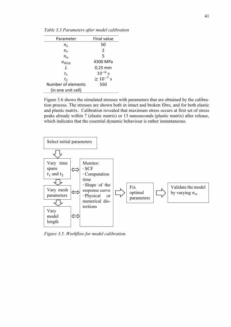
41

Table 3.3 Parameters after model calibration

Figure 3.6 shows the simulated stresses with parameters that are obtained by the calibra-

tion process. The stresses are shown both in intact and broken fibre, and for both elastic

and plastic matrix. Calibration revealed that maximum stress occurs at first set of stress

peaks already within 7 (elastic matrix) or 13 nanoseconds (plastic matrix) after release,

which indicates that the essential dynamic behaviour is rather instantaneous.

Figure 3.5. Workflow for model calibration.

Parameter Final value

𝑛𝐿 50 𝑛𝑟 2 𝑛𝑢 5 𝜎𝑑𝑖𝑠𝑝 4300 MPa

𝐿 0.25 mm 𝑡1 10−6 s 𝑡2 ≥ 10−7 s

Number of elements (in one unit cell)

550

Select initial parameters

Vary time

spans

𝑡1 and 𝑡2

Vary mesh

parameters

Vary

model

length

Validate the model

by varying 𝜎∞

Fix

optimal

parameters

Monitor:

∙ SCF

∙ Computation

time

∙ Shape of the

response curve

∙ Physical or

numerical dis-

tortions

42

Figure 3.6. Simulated stresses with parameter values obtained by the calibration process.

Stresses are recorded at 𝑥 = 0 in broken fibre and closest intact fibre, and for both elastic

and plastic matrix.

𝜎𝑚𝑎𝑥,𝑒𝑙𝑎𝑠𝑡𝑖𝑐

𝜎𝑚𝑎𝑥,𝑝𝑙𝑎𝑠𝑡𝑖𝑐

𝜎∞

Max stress/SCF

Broken fibre

43

3.2.1 Step time calibration

Firstly, goal was to select appropriate time parameters 𝑡1 and 𝑡2 and corresponding time

spans for simulations. Time spans were minimized by satisfying following criteria:

- 𝑡1: No significant stress oscillations while applying smooth step transition.

- 𝑡2: Time span should be sufficiently large to be able to capture maximum physical

stress peak.

Initial values for 𝑡1 and 𝑡2 were determined by studying speed of stress waves in fibre and

matrix. The starting point for appropriate time span determination was the longitudinal

stress wave propagation in carbon fibre. Since CFRP structure is significantly larger in

reality, stress waves would not actually reflect from the boundaries of the model with

limited geometric dimensions. These reflections may cause non-physical stress oscilla-

tions. Therefore, focus is on the first sets of peaks since model is relatively small. In

addition, it must be confirmed that after the smooth step loading, the remote stress has

been settled and applied to all elements. If the smooth step loading period is too small,

fibre is released before desired stress state is achieved at crucial locations. Moreover, it

must be monitored that smooth step loading period will not cause significant structural

oscillations.

Firstly, step time 𝑡1 was determined. For model parameters (T800H/3631) retrieved from

FE model by St-Pierre et al. (2017) and by adapting the expression (2.27) speed of max-

imum longitudinal stress wave propagation is defined by

𝑐𝑓 = (𝐸𝑓

𝜌𝑓)

1

2

= (294 GPa

1,8 g

cm3

)

1

2

= 12780m

s. (3.6)

Hence, a minimum time for longitudinal stress wave to travel from 𝑥 = 0 to 𝑥 = 𝐿 is

defined by

𝑡𝐿 =𝐿

𝑐𝑓= 7,82 ∙ 10−5 ∙ 𝐿 (

s

m) . (3.7)

Formula (3.7) assumes unconstrained propagation of stress wave and neglects the effect

of matrix damping. Nevertheless, it provides information of the magnitude of stress wave

speed and can be used for a reference time. Since tensile modulus for matrix is lower than

for the fibre, 𝑐𝑓 represents maximum value for stress wave propagation speed in the whole

structure. Since the final model length 𝐿 may differ from the initial value of 0.5 m, the

stress state build-up must be confirmed also for larger models. For example, if 𝐿 =2.0 mm which is significantly larger than quasi-static model with a length of 𝐿 = 0.75

mm, the absolute minimum time for 𝑡1 is 0.16 microseconds. Therefore, the values for 𝑡1

should be at least equal or larger than 1 μs. Figure 3.7 shows the smooth step transition

for model length 𝐿 = 0.5 mm for Step 1 for step times 𝑡1 = 1 μs and 10 μs, and for com-

parison step time 𝑡1 = 0.1 μs. Results show clearly that step time 𝑡1 = 10−7 s leads

clearly to undesired increase of stress while the final stress level should be 4300 MPa.

Stresses by step times 𝑡1 = 1 μs and 10 μs appear to follow the shape of prescribed dis-

placement curve. To minimize computation time, step time 𝑡1 = 1 μs was fixed for the

remaining simulations, and larger step times were only used if verification was needed.

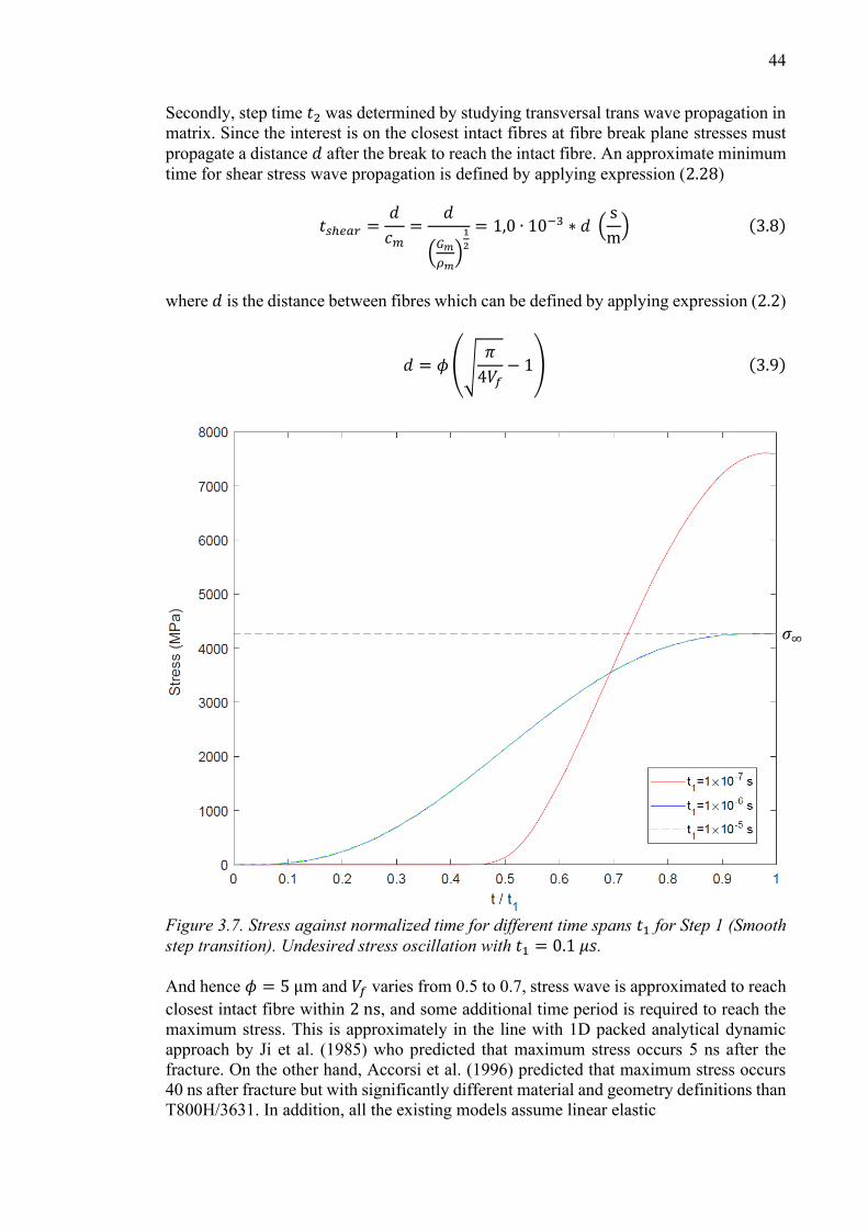
44

Secondly, step time 𝑡2 was determined by studying transversal trans wave propagation in

matrix. Since the interest is on the closest intact fibres at fibre break plane stresses must

propagate a distance 𝑑 after the break to reach the intact fibre. An approximate minimum

time for shear stress wave propagation is defined by applying expression (2.28)

𝑡𝑠ℎ𝑒𝑎𝑟 =𝑑

𝑐𝑚=

𝑑

(𝐺𝑚

𝜌𝑚)

1

2

= 1,0 ∙ 10−3 ∗ 𝑑 (s

m) (3.8)

where 𝑑 is the distance between fibres which can be defined by applying expression (2.2)

𝑑 = 𝜙(√𝜋

4𝑉𝑓− 1) (3.9)

Figure 3.7. Stress against normalized time for different time spans 𝑡1 for Step 1 (Smooth

step transition). Undesired stress oscillation with 𝑡1 = 0.1 𝜇𝑠.

And hence 𝜙 = 5 μm and 𝑉𝑓 varies from 0.5 to 0.7, stress wave is approximated to reach

closest intact fibre within 2 ns, and some additional time period is required to reach the

maximum stress. This is approximately in the line with 1D packed analytical dynamic

approach by Ji et al. (1985) who predicted that maximum stress occurs 5 ns after the

fracture. On the other hand, Accorsi et al. (1996) predicted that maximum stress occurs

40 ns after fracture but with significantly different material and geometry definitions than

T800H/3631. In addition, all the existing models assume linear elastic

𝜎∞

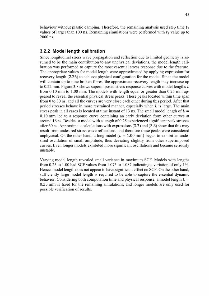
45

behaviour without plastic damping. Therefore, the remaining analysis used step time 𝑡2

values of larger than 100 ns. Remaining simulations were performed with 𝑡2 value up to

2000 ns.

3.2.2 Model length calibration

Since longitudinal stress wave propagation and reflection due to limited geometry is as-

sumed to be the main contribution to any unphysical deviations, the model length cali-

bration was performed to capture the most essential stress response due to the fracture.

The appropriate values for model length were approximated by applying expression for

recovery length (2.26) to achieve physical configuration for the model. Since the model

will contain up to nine broken fibres, the approximate recovery length may increase up

to 0.22 mm. Figure 3.8 shows superimposed stress response curves with model lengths 𝐿

from 0.10 mm to 1.00 mm. The models with length equal or greater than 0.25 mm ap-

peared to reveal the essential physical stress peaks. These peaks located within time span

from 0 to 30 ns, and all the curves are very close each other during this period. After that

period stresses behave in more restrained manner, especially when 𝐿 is large. The main

stress peak in all cases is located at time instant of 13 ns. The small model length of 𝐿 =0.10 mm led to a response curve containing an early deviation from other curves at

around 16 ns. Besides, a model with a length of 0.25 experienced significant peak stresses

after 60 ns. Approximate calculations with expressions (3.7) and (3.8) show that this may

result from undesired stress wave reflections, and therefore these peaks were considered

unphysical. On the other hand, a long model (𝐿 = 1.00 mm) began to exhibit an unde-

sired oscillation of small amplitude, thus deviating slightly from other superimposed

curves. Even longer models exhibited more significant oscillations and became seriously

unstable.

Varying model length revealed small variance in maximum SCF. Models with lengths

from 0.25 to 1.00 had SCF values from 1.075 to 1.087 indicating a variation of only 1%.

Hence, model length does not appear to have significant effect on SCF. On the other hand,

sufficiently large model length is required to be able to capture the essential dynamic

behavior. Considering both computation time and physical response, a model length 𝐿 =0.25 mm is fixed for the remaining simulations, and longer models are only used for

possible verification of results.

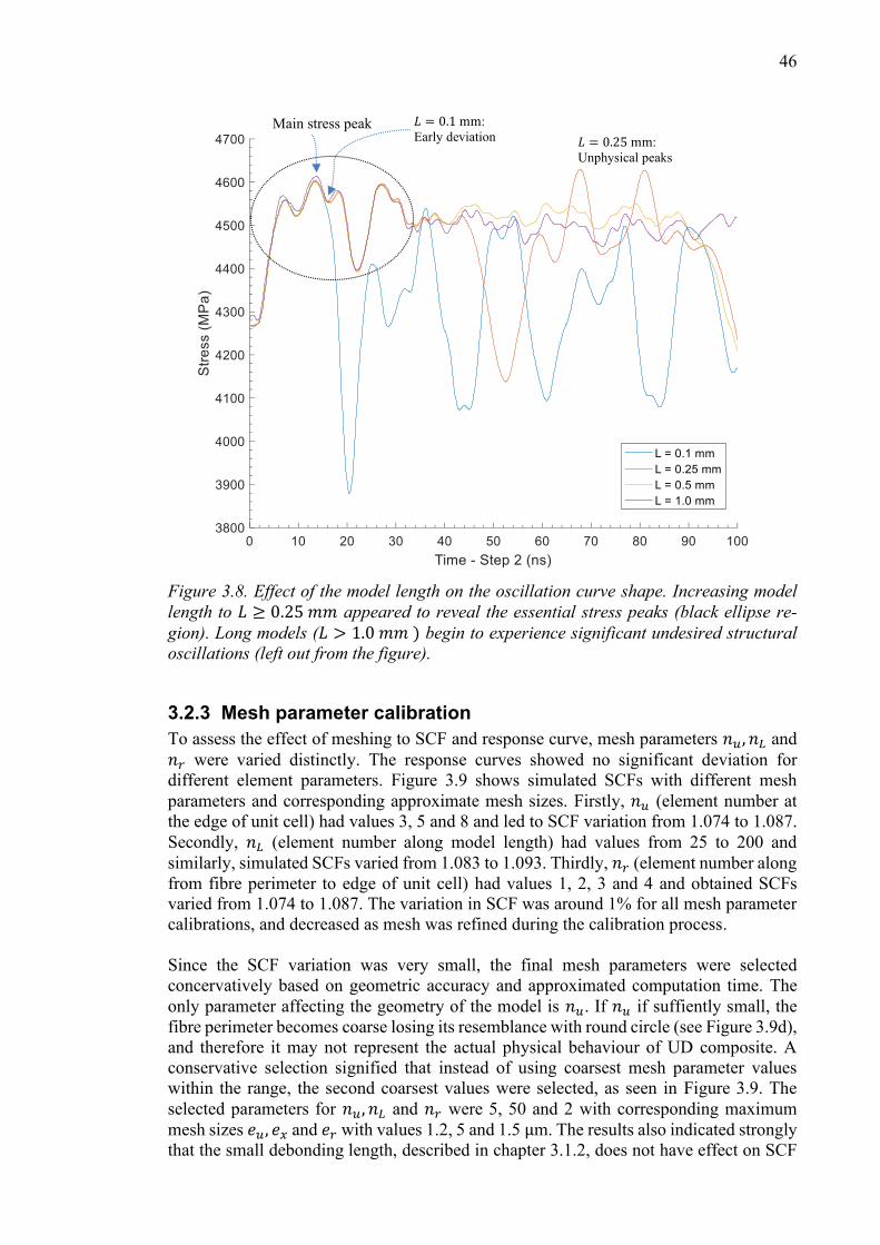
46

Figure 3.8. Effect of the model length on the oscillation curve shape. Increasing model

length to 𝐿 ≥ 0.25 𝑚𝑚 appeared to reveal the essential stress peaks (black ellipse re-

gion). Long models (𝐿 > 1.0 𝑚𝑚 ) begin to experience significant undesired structural

oscillations (left out from the figure).

3.2.3 Mesh parameter calibration

To assess the effect of meshing to SCF and response curve, mesh parameters 𝑛𝑢, 𝑛𝐿 and

𝑛𝑟 were varied distinctly. The response curves showed no significant deviation for

different element parameters. Figure 3.9 shows simulated SCFs with different mesh

parameters and corresponding approximate mesh sizes. Firstly, 𝑛𝑢 (element number at

the edge of unit cell) had values 3, 5 and 8 and led to SCF variation from 1.074 to 1.087.

Secondly, 𝑛𝐿 (element number along model length) had values from 25 to 200 and

similarly, simulated SCFs varied from 1.083 to 1.093. Thirdly, 𝑛𝑟 (element number along

from fibre perimeter to edge of unit cell) had values 1, 2, 3 and 4 and obtained SCFs

varied from 1.074 to 1.087. The variation in SCF was around 1% for all mesh parameter

calibrations, and decreased as mesh was refined during the calibration process.

Since the SCF variation was very small, the final mesh parameters were selected

concervatively based on geometric accuracy and approximated computation time. The

only parameter affecting the geometry of the model is 𝑛𝑢. If 𝑛𝑢 if suffiently small, the

fibre perimeter becomes coarse losing its resemblance with round circle (see Figure 3.9d),

and therefore it may not represent the actual physical behaviour of UD composite. A

conservative selection signified that instead of using coarsest mesh parameter values

within the range, the second coarsest values were selected, as seen in Figure 3.9. The

selected parameters for 𝑛𝑢, 𝑛𝐿 and 𝑛𝑟 were 5, 50 and 2 with corresponding maximum

mesh sizes 𝑒𝑢, 𝑒𝑥 and 𝑒𝑟 with values 1.2, 5 and 1.5 μm. The results also indicated strongly

that the small debonding length, described in chapter 3.1.2, does not have effect on SCF

Main stress peak 𝐿 = 0.1 mm:

Early deviation 𝐿 = 0.25 mm:

Unphysical peaks

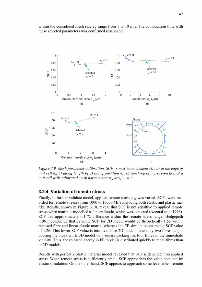
47

within the considered mesh size 𝑒𝑥 range from 1 to 10 μm. The computation time with

these selected parameters was confirmed reasonable.

Figure 3.9. Mesh parameter calibration. SCF vs maximum element size a) at the edge of

unit cell 𝑒𝑢 b) along length 𝑒𝐿 c) along partition 𝑒𝑟. d) Meshing of a cross-section of a

unit cell with calibrated mesh parameters: 𝑛𝑢 = 5, 𝑛𝑟 = 2.

3.2.4 Variation of remote stress

Finally, to further validate model, applied remote stress 𝜎∞ was varied. SCFs were rec-

orded for remote stresses from 1000 to 10000 MPa including both elastic and plastic ma-

trix. Results, shown in Figure 3.10, reveal that SCF is not sensitive to applied remote

stress when matrix is modelled as linear elastic, which was expected (Accorsi et al. 1996).

SCF had approximately 0.1 % difference within the remote stress range. Hedgepeth

(1961) conducted that dynamic SCF for 2D model would be theoretically 1.53 with 1

released fibre and linear elastic matrix, whereas the FE simulation estimated SCF value

of 1.26. This lower SCF value is intuitive since 2D models have only two fibres neigh-

bouring the break while 3D model with square packing has four fibres in the immediate

vicinity. Thus, the released energy in FE model is distributed quickly to more fibres than

in 2D models.

Results with perfectly plastic material model revealed that SCF is dependent on applied

stress. When remote stress is sufficiently small, SCF approaches the value obtained by

elastic simulation. On the other hand, SCF appears to approach some level when remote

𝑛𝑢 = 3 𝑛𝑢 = 8

𝑛𝑟 = 4

𝑛𝑟 = 1

Selected 𝑛𝑢 = 5

Selected 𝑛𝑟 = 2

Selected 𝑛𝐿 = 50

a) b)

c) d)

𝑛𝐿 = 200

𝑛𝐿 = 25

48

stress increases. This type of behaviour in SCF was also concluded by Hedgepeth and van

Dyke (1967) in their simplified 2D static plastic model (see Figure 2.16). As mentioned

previously, there are currently no dynamic models to which compare and assess the effect

of plasticity. Nevertheless, this model obtained a SCF value of 1.08 for nominal remote

stress (4300 MPa) which is in relative terms 14% lower than for elastic matrix.

Figure 3.10. Dynamic SCF against input remote stress for elastic and plastic matrix.

49

4 Results and discussion

The main aim of the dynamic finite element model was to obtain the maximum dynamic

SCF following the fibre fracture. This chapter shows the obtained dynamic SCFs against:

i) the number of broken fibres 𝑛𝑏, ii) shape of the broken region and iii) fibre volume

fraction 𝑉𝑓. The broken fibres were arranged either in a square (1, 4 and 9 broken fibres)

or row shape (2,3 and 4 broken fibres). In addition, the sensitivity of matrix material

model to SCF was assessed in each case. In all cases, the maximum stresses occurred at

the intact fibre closest to the broken fibre region, as seen in Figure 4.1. The computation

with a standard desktop computer varied from 5 minutes to 1 hour depending on the size

of the model or the number of elements (~104 to 105 elements).

The shape of the response curves for more than one released fibre revealed no significant

difference to response curve for one broken fibre (see Figure 3.6). On the other hand, the

results showed that the maximum stress occurs later if the size of the bundle is increased.

The time instant for maximum stress had values 13, 19 and 39 ns for one, four and nine

broken fibres in square arrangement with perfectly plastic matrix. When the matrix was

modelled as linear elastic, the corresponding time instants were 7, 8 and 11 ns. When

fibres broke in a row, the main stress peak was achieved before 22 ns.

Figure 4.1. Location of maximum stress (green circle) at fibre break plane (𝑥 = 0) for

different arrangements of broken fibres (red region).

4.1 Effect of number of broken fibres

Figure 4.2 shows simulated dynamic SCF for different number of broken fibres. In addi-

tion, it shows corresponding quasi-static results by St-Pierre et al. (2017). Each simulation

was established by increasing the total number of fibres, i.e. the bundle size, and by mon-

itoring the convergence of SCF. During this establishment the model incorporated per-

fectly plastic matrix material model. Bundle size was increased in a such way that the

broken region was always located at the centre of the bundle to achieve symmetry. Con-

vergence study was finished when the difference in SCF between consecutive increments

was less than 0.5%. This bundle size was then fixed for the simulations with other param-

eters. The establishment process was repeated distinctly for each number of broken fibres.

The convergence was achieved at relatively small bundles: 49 for one broken fibre, 100

for four released fibres and 169 for nine released fibres. For example, for one broken

fibre, SCF decreased only from 1.083 to 1.074 when bundle size was increased from 25

to 125.

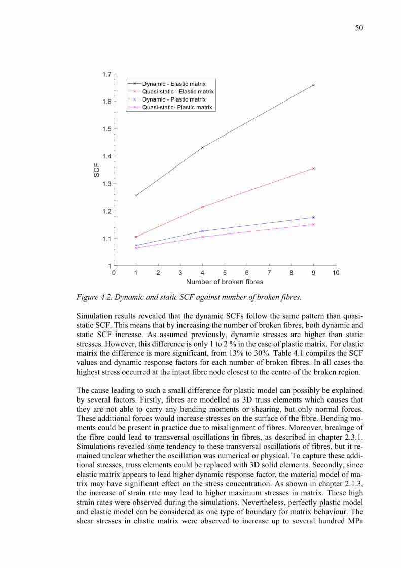
50

Figure 4.2. Dynamic and static SCF against number of broken fibres.

Simulation results revealed that the dynamic SCFs follow the same pattern than quasi-

static SCF. This means that by increasing the number of broken fibres, both dynamic and

static SCF increase. As assumed previously, dynamic stresses are higher than static

stresses. However, this difference is only 1 to 2 % in the case of plastic matrix. For elastic

matrix the difference is more significant, from 13% to 30%. Table 4.1 compiles the SCF

values and dynamic response factors for each number of broken fibres. In all cases the

highest stress occurred at the intact fibre node closest to the centre of the broken region.

The cause leading to such a small difference for plastic model can possibly be explained

by several factors. Firstly, fibres are modelled as 3D truss elements which causes that

they are not able to carry any bending moments or shearing, but only normal forces.

These additional forces would increase stresses on the surface of the fibre. Bending mo-

ments could be present in practice due to misalignment of fibres. Moreover, breakage of

the fibre could lead to transversal oscillations in fibres, as described in chapter 2.3.1.

Simulations revealed some tendency to these transversal oscillations of fibres, but it re-

mained unclear whether the oscillation was numerical or physical. To capture these addi-

tional stresses, truss elements could be replaced with 3D solid elements. Secondly, since

elastic matrix appears to lead higher dynamic response factor, the material model of ma-

trix may have significant effect on the stress concentration. As shown in chapter 2.1.3,

the increase of strain rate may lead to higher maximum stresses in matrix. These high

strain rates were observed during the simulations. Nevertheless, perfectly plastic model

and elastic model can be considered as one type of boundary for matrix behaviour. The

shear stresses in elastic matrix were observed to increase up to several hundred MPa

51

which is significantly higher than 52.4 MPa, which is the limit shear stress in linear elastic

perfectly plastic model.

Table 4.1. Dynamic SCF and dynamic response factor in quasi-static and dynamic simu-

lation for both linear elastic matrix and linear elastic perfectly plastic matrix.

Number of

broken fibres

SCF Quasi-static SCF Dynamic Dynamic response factor 𝜂𝑟

Plastic Elastic Plastic Elastic Plastic Elastic

1 1.07 1.11 1.07 1.26 1.01 1.13

4 1.11 1.22 1.13 1.43 1.02 1.18

9 1.15 1.36 1.18 1.66 1.02 1.22

4.2 Fibres breaking in a row

Figure 4.3 shows SCF with different number of broken fibres when broken fibres are

arranged in a row. The bundle size was determined in a such way that at least equal num-

ber of intact fibres should locate between the broken section and the borders of the model

than in the corresponding model with square shaped broken region. In addition, broken

region was similarly placed at the centre of the bundle. For example, a row of four broken

fibres was placed in 10 by 7 bundle. As in the case of square shaped broken region, the

highest stress occurred at the intact fibre node closest to the centre of the broken region.

Compared to results from the 1D packed linear elastic model by Hedgepeth (1961), dy-

namic SCFs are smaller and the location of highest stress was different. Hedgepeth pre-

dicted relatively from 21 % to 55 % of increase in SCF for 1, 2 and 3 broken fibres. The

location for maximum stress in Hedgepeth’s model was naturally the intact fibre follow-

ing the row of broken fibres, while in this 2D packed model it represented the location of

lowest SCF of adjacent fibres (see Figure 3.4c). Considering for example one broken fibre

there are some natural differences between 1D regular and 2D square packing. In the

model of Hedgepeth, each fibre is immediately surrounded by two fibres whereas 2D

square packing leads to four fibres in the vicinity of the broken fibre. On the other hand,

considering some distance 𝑟, the number of intact fibres within this region is increases

proportional to 𝑟2 in 2D packing, whereas in 1D packing the increase is linear with re-

spect to 𝑟. Therefore, it is challenging to compare these results straight.

However, these results may give a clue of the order in which the fibres will fail. Consid-

ering both square and row arranged broken fibres, the results indicate that broken region

tends to grow towards a circular arrangement of broken fibres. On the other hand, the

actual observed co-planar clusters have both features of circular formation and propaga-

tion along a narrow path, as seen in Figure 2.5 in chapter 2.1.3. Actual bundles are ran-

domly packed which might lead to a different sequence of breaks than square packed

model. In addition, statistical treatment of stresses in the neighbourhood would provide a

prediction of the break propagation type but it is beyond the scope of this study.

52

Figure 4.3. Dynamic SCF against number of broken fibres when fibres are arranged in a

row. For comparison: Hedgepeth’s (1961) elastic 1D packed model and SCFs for square

shaped broken region (𝑛𝑏 = 4).

4.3 Effect of fibre volume fraction

Figure 4.4 shows SCF with different values of fibre volume fraction and corresponding

distance between fibre surfaces. Fibre volume fraction values were varied from 0.4 to

0.75 while actual values lie typically within 0.5 to 0.6. However, varying fibre volume

fraction affects naturally to element sizes, as seen in expressions (3.2) and (3.3). For ex-

ample, 𝑉𝑓 = 0.75 leads to minimum radial mesh size 𝑒𝑟 of 0.03 μm while 𝑉𝑓 = 0.4 leads

to minimum radial mesh size 𝑒𝑟 of 0.5 μm (see expression 3.2), even though the number

of elements in a unit cell was the same. Therefore, results were verified by converging

the mesh which revealed no significant difference compared to original results. The anal-

ysis was performed only for one broken fibre. When fibre volume fraction is increased,

SCF appears to decrease for both elastic and plastic matrix material models. For plastic

matrix, SCF decreased from 1.10 to 1.05 for fibre volume fraction values from 0.4 to

0.75, corresponding a 5% decrease in SCF. For elastic matrix, the decrease was more

restrained but apparent.

This decrease in SCF is in contradict with the results from quasi-static simulations

(Swolfs et al. 2015) which obtained that static stress concentration factor increases when

distance 𝑑 between fibres decreases, as seen in Figure 2.18. However, since dynamic

stresses of fibre are different and not very well known for 2D packed models, this contra-

dict does not necessary indicate that there is an error in model definition. Swolfs et al.

also utilized random packing which leads to different distribution of SCF in the neigh-

bourhood of broken fibre. As compared in chapter 2.4, random packing might lead to

53

locally higher SCF, at least in static analysis. The decrease in SCF is also slightly contra-

dict with the dynamic 1D packed model by Hedgepeth (1961) which assumed that SCF

is independent of 𝑑. On the other hand, it is rather intuitive that high fibre volume fraction

might lead to decrease in SCF, since the higher fibre volume fraction indicates that neigh-

bouring fibres are closer to the break point. This implies that the released stress will prop-

agate faster from fibre to another which could even the stresses in the neighbourhood of

the broken fibre. In addition, in 2D packed models, stresses can propagate along the ma-

trix past fibres, while in 1D packed models the stress wave needs to travel through the

fibre. Furthermore, quasi-static models do not include this stress propagation effect.

Figure 4.4. Dynamic SCF against fibre volume fraction and corresponding distance be-

tween fibres.

4.4 Discussion

This section assesses results from two different perspectives. First subchapter discusses

of the model input data, including material properties and input geometry. Second sub-

chapter discusses of the technical modelling aspects, such as element definitions and frac-

ture simulation.

4.4.1 Input data

Material model of matrix appeared to have significant impact on SCF. Linear elastic ma-

trix caused significantly higher dynamic response factor (1.12 to 1.22) than linear elastic

perfectly plastic matrix (only 1.01 to 1.02), which indicates that only linear elastic matrix

behaviour would emphasise the increase of SCF due to dynamic stresses. However, these

models were essentially different since linear elastic model did not have maximum stress

limit, which led to probably unrealistically high stresses during the simulation. On the

other hand, there is actually limited amount reliable material data for this setup, as de-

scribed in chapter 2.1.4. Material models should be applicable both for microscale resin

(fibre spacing < few μm) and for high strain rates (dynamic fracture). Despite the lack of

knowledge, one could attempt to modify matrix material models, such as by incorporating

linear hardening or by increasing the yield limit. Fibres were modelled as linear elastic

𝑑 = 0.1 μm

𝑑 = 2 μm

𝑑 = 𝑑(𝑉𝑓)

𝑑 = 0.7 μm

𝑑 = 0.5 μm 𝑑 = 1.2 μm

54

instead of slightly non-linear elastic, but this rather accurate approximation was consid-

ered not the main source of error. To reliably predict the co-planar failure, one should be

able to obtain strength for a fibre element of a few μm. This strength approximation on

short fibre element is beyond the scope of this study but would be important to consider

in the future.

The input geometry of the model can be defined by four main parameters: fibre diameter,

bundle size, packing type and fibre volume fraction. Currently, the fibre volume fraction

𝑉𝐹 seem to have a small, but noteworthy, effect on dynamic SCF. Dynamic SCF appears

to consistently decrease when fibre volume fraction increases, i.e. the distance between

fibres 𝑑 decreases, which is slightly contradict with the quasi-static results (see Figure

2.18). In general, fibre diameter and bundle size of the model had a minor effect on dy-

namic SCF. Fibre diameter 𝜙 has a small variation in reality (Yu and Yao 2006), thus an

assumption on constant diameter is justified. The computational resources enabled large

bundle sizes 𝑛𝑡 and model length 𝐿, and their effect on dynamic SCF was negligible when

the model geometry was sufficiently large. In addition, a relatively small model was able

to capture the essential dynamic behaviour. The average static SCF in composite was not

dependent on the packing type (random, square, hexagonal), but when dynamics are in-

corporated, this conclusion might not be valid. In random packing, dynamic stressed

might overconcentrate on the closest fibres due to limited stress wave propagation speed

and thereby increasing the probability of the initiation of rapid cluster formation.

4.4.2 Modelling aspects

The modelling of the fibre elements is considered one of the main factors affecting the

SCF. Currently, fibres are one dimensional line elements carrying only uniform normal

forces. To be able to capture more versatile mechanical behaviour, such as shearing, bend-

ing and transversal oscillation, fibres could be modelled as 3D solid elements. Conse-

quently, 3D elements would capture the variation of SCF across the cross-section of fibre.

On the other hand, modelling the fibres as transversely infinitely stiff was not considered

to have significant effect on results.

The small debonding near fracture did not have an impact on SCF. Also, the perfect bond-

ing on fibre/matrix interface was deduced to be a realistic assumption. Therefore, it is

assumed that incorporated friction or adhesive elements at matrix/fibre interface would

not affect significantly on SCF.

Mesh density of this model was not observed to limit the accuracy of the obtained SCF.

Mesh refinement did not provide more accurate results after certain mesh size, and the

used meshing did not distort the model geometry (circular fibre perimeter). In addition,

the fibre elements were shorter than co-planar crack distance between adjacent fibres.

Even though relatively fine mesh was applied everywhere in the model, the computation

times were reasonable since the model geometry was rather small. However, the rapid

dynamic effects were concentrated at relatively small region in the model. Thus, the mesh

could be optimized especially if one will use such modelling techniques that would re-

quire large number of elements near the break.

The model simulated the fracture by releasing the broken fibres at the same time. This

method contains two unphysical assumptions. Firstly, consecutive fibre breaks could oc-

cur approximately 3 to 20 ns from each other. However, based on results on 1D packed

55

models (Hedgepeth 1961, Accorsi et al. 1996), this is not expected to have significant

effect on SCF, but could be verified for 2D packed models. Secondly, current modelling

does not take into account the energy that is required to form a crack in fibres and matrix.

Consequently, the model does not properly incorporate stress concentrations at the crack

tip near the fibre. This approach would possibly obtain more realistic results.

56

5 Conclusions

The aim of the thesis was to assess whether dynamic stresses are sufficiently high to ex-

plain the prevalence of co-planar breaks in a unidirectional composite. This process was

divided in two main steps. First, a literature review was performed to discover relevant

data related to composites and existing stress predictions by current static and dynamic

models. Then, an improved numerical model was constructed and validated to simulate

dynamic stresses, or dynamic stress concentration factor (SCF), due to breakage. The

model of this thesis utilized dynamic explicit finite element method in Abaqus 2017/CAE

software. Finally, results were compared to current static and dynamic models, and the

sensitivity of different factors on dynamic SCF was determined.

The model assessed the impact on dynamic SCF of following main factors:

- Number of broken fibres (1 to 9 broken fibres)

- Shape of the broken region (square or row)

- Volume fraction of fibres (0.4 to 0.75)

- Material model of matrix resin for each case above (linear elastic or linear elastic

perfectly plastic)

Simulation results showed consistently that dynamic stresses due to fracture are higher

than static stresses for similar setup. In addition, this difference increased further when

the size of the broken bundle increased. However, the dynamic stresses were only 1 to 2

% larger than static stresses when matrix was assumed behave in a linear elastic perfectly

plastic manner which is currently relatively feasible assumption on constitutive behaviour

of the matrix. If the increase of stress due to dynamic behaviour can be verified this small,

the primary cause of co-planar clusters is not the dynamic SCF. On the other hand, dy-

namic stresses were 12 to 23 % larger for linear elastic matrix which may not represent

the actual physical behaviour of matrix. Dynamic simulations on a row of broken fibres

revealed two trends. Firstly, the row arrangement of broken fibres was shown to lead to

slightly higher dynamic SCF than square arranged broken bundle with same number of

broken fibres. Secondly, simulations indicated that the broken section (row shape) tends

slightly to grow in a circular shape instead of growing in the direction of the row. The

results also showed that if fibres are closer to each other, i.e. the fibre volume fraction is

higher, the dynamic SCF may decrease for up to 5 %. This decrease is slightly in contra-

dict with the quasi-static simulations (see Figure 2.16) and did not significantly depend

on material model of matrix.

Overall, this thesis conducted following main conclusions:

- Matrix material model has a significant contribution to dynamic SCF.

- The higher fibre volume fraction leads to slightly lower dynamic SCF.

- Dynamic stresses become more important when the number of broken fibres is

increased.

This thesis constructed first 3D FE model setup incorporating dynamic effects such as

dynamic stress propagation. Even though there are some open questions related to the

modelling aspects and accuracy of simulation, this current model might be beneficial

framework for future studies. The simulations also concluded that dynamic effects seem

rather local and rapid. Therefore, it might be sufficient to have relatively small models

(bundle size, model length) and short simulation time spans, i.e. time after release).

57

Based on literature review, results and authors personal views, following actions are rec-

ommended for the future work. Recommendations favour the methods that are easy to

implement or would possibly enhance the model remarkably:

- Applying different material models for matrix. Assessing the effect of hardening,

linearity and yield stress.

- Setting fibres to break within a small delay.

- Verifying the results by applying random packing.

- Modelling fibres by 3D solid elements instead of 1D truss elements.

- Applying fracture mechanics approach.

Finally, this thesis emphasizes two main approaches for future studies. Firstly, the most

straightforward step would be the implementation of different matrix material models.

Determination of sensitivity of matrix yield strain to dynamic SCF or application of linear

hardening model would obtain important additional data on matrix dynamic behaviour.

Secondly, fibres could be modelled as 3D-elements to enable more versatile dynamic

behaviour. This enhancement would allow to fibres bend or vibrate transversally after the

break and would enable the model to capture even more localized stresses. Even if it is

currently difficult to assess the importance of the local stresses, the comparison with cor-

responding quasi-static models could provide additional way to determine the stress in-

crease due to dynamics.

58

References

Abaqus (2013), Online Documentation. Dassault Systèmes Simulia Corp. , Providence,

Rhode Island, USA

Accorsi M. L. , Pegoretti A. , Dibenedetto A. T. 1996. Dynamic analysis of fibre break-

age in single- and multiple-fibre composites. Journal of Material Science. Vol. 31(16).

pp. 4181–4187. Available at https://doi.org/10.1007/BF00356437 ISSN: 0022-2461

(Print) 1573-4803 (Online)

Behzadi A. , Paul T. , Curtis B. , Frank R. Jones A. 2009. Improving the prediction of

tensile failure in unidirectional fibre composites by introducing matrix shear yielding.

Composites Science and Technology. Vol. 69(14). pp. 2421-2427. Available at

https://doi.org/10.1016/j.compscitech.2009.06.010 ISSN: 0266-3538

Beyerlein I. J. , Phoenix S. L. 1996a. Statistics for the strength and size effects of micro-

composites with four carbon fibers in epoxy resin. Composites Science and Technology.

Vol. 56(1). pp. 75–92. Available at https://doi.org/10.1016/0266-3538(95)00131-X

ISSN: 0266-3538

Beyerlein I. J. , Phoenix S. L. 1996b. Stress concentrations around multiple fiber breaks

in an elastic matrix with local yielding or debonding using quadratic influence superpo-

sition. Journal of the Mechanics and Physics of Solids. Vol. 44(12). pp. 1997–2039.

Available at https://doi.org/10.1016/S0022-5096(96)00068-3 ISSN: 0022-5096

Blassiau S. , Thionnet A. , Bunsell A. R. 2006. Micromechanisms of load transfer in a

unidirectional carbon fibre-reinforced epoxy composite due to fibre failures. Part 2: in-

fluence of viscoelastic and plastic matrices on the mechanisms of load transfer. Compo-

site Structures. Vol 74(3). pp. 319–331. ISSN: 0263-8223

Callens M. G. , Gorbatikh L. , Verpoest I. 2014. Ductile steel fibre composites with brit-

tle and ductile matrices. Composites Part A: Applied Science and Manufacturing. Vol.

61. pp. 235-244. Available at https://doi.org/10.1016/j.compositesa.2014.02.006 ISSN:

1359-835X

Cornelia J. , Wärmefjord K. , Cromvik C. , Söderberg R. , Lindkvist, L. , Carlson J. ,

Larsson S. , Edelvik F. 2016. Geometry Assurance Integrating Process Variation with

Simulation of Spring-In for Composite Parts and Assemblies. Journal of Computing and

Information Science in Engineering. Vol 16(3) Available at

https://doi.org/10.1115/IMECE2014-38228 ISSN: 1530-9827 (print) 1944-7078

(online)

Curtis G. J. , Milne J. M. , Reynolds W. N. 1968. Non-Hookean Behaviour of Strong

Carbon Fibres. Nature. Vol. 220. pp. 1024-1025. Available at

https://doi.org/10.1038/2201024a0 ISSN: 1476-4687 (online)

Fiedler B. , Klisch A. , Schulte K. 1998. Stress concentrations in multiple fibre model

composites. Composites Part A: Applied Science and Manufacturing. Vol. 29(9–10).

pp. 1013–1019. Available at https://doi.org/10.1016/S1359-835X(98)00014-1 ISSN:

1359-835X

59

Giannotti M. I. , Galante M. J. , Oyanguren P. A. , Vallo C. I. 2003. Role of intrinsic

flaws upon flexural behaviour of a thermoplastic modified epoxy resin. Polymer Test-

ing. Vol.22(4). pp.429–437. Available at https://doi.org/10.1016/S0142-9418(02)00124-

1 ISSN: 0142-9418

Harikrishnan P. , Mohite M. , Upadhyay C. S. 2018. Generalized Weibull model-based

statistical tensile strength of carbon fibres. Archive of Applied Mechanics. Vol. 88(9).

pp. 1617-1636. Available at https://doi.org/10.2514/6.2015-0972 ISSN: 0939-1533

(Print) 1432-0681 (Online)

Hedgepeth J. M. 1961. Stress concentrations in filamentary structures. NASA Technical

Note. D-882. pp. 1-36 Available at

https://ntrs.nasa.gov/archive/nasa/casi.ntrs.nasa.gov/19980227450.pdf

Hedgepeth J. M. , Van Dyke P. 1967. Local stress concentrations in imperfect

filamentary composite materials. Journal of Composite Materials. Vol. 1(3). pp. 294-

309. Available at https://doi.org/10.1177/002199836700100305 ISSN: 0021-9983

Heuvel P. W. J. , Goutianos S. , Young R. J. , Peijs T. 2004. Failure phenomena in fi-

bre-reinforced composites. Part 6: a finite element study of stress concentrations in uni-

directional carbon fibre-reinforced epoxy composites. Composites Science and Technol-

ogy. Vol. 64(5). Pp. 645-656. Available at https://doi.org/10.1016/j.comp-

scitech.2003.06.003 ISSN: 0266-3538

Heuvel P. W. J. , Wubbolts M. K. , Young R. J. , Peijs T 1998. Failure phenomena in

twodimensional multi-fibre model composites: 5. A finite element study. Composites

Part A: Applied Science and Manufacturing. Vol. 29(9-10). pp. 1121–1135. Available

at https://doi.org/10.1016/S1359-835X(98)00089-X ISSN: 0266-3538

Hinton M. J. & Kaddour A. S., Soden P. D. 2004. Evaluation of failure prediction in

composite laminates: background to ‘part C’ of the exercise. Composites Science and

Technology, Vol. 63:3-4. Pp. 321-327. Available at https://doi.org/10.1016/S0266-

3538(03)00216-1 ISSN: 0266-3538

Hinton M. J. , Soden P. D. 1998. Predicting failure in composite laminates: the

background to the exercise. Composite Science and Technology. Vol. 58(7). pp. 1001–

1010. Available at https://doi.org/10.1016/S0266-3538(98)00074-8 ISSN: 0266-3538

Ji X. , Liu X.R. , Chou T. W. 1985. Dynamic stress concentration factors in unidirec-

tional composites. Journal of Composite Materials, Vol. 19:3. pp. 269–75. Available at

https://doi.org/10.1177/002199838501900305 ISSN: 0021-9983

Kaddour A. S. , Hinton M. J. 2013. Maturity of 3D failure criteria for fibre-reinforced

composites: comparison between theories and experiments: Part B of WWFEII. Journal

of Composite Materials. Vol. 47(6–7). pp.925–966. Available at

https://doi.org/10.1177/0021998313478710 ISSN: 0021-9983

Landis C. M. , McMeeking R. M. 1999. Stress concentrations in composites with inter-

face sliding, matrix stiffness and uneven fiber spacing using shear lag theory. Interna-

tional Journal of Solids and Structures. Vol. 36(28). pp. 4333–4361. Available at

https://doi.org/10.1016/S0020-7683(98)00193-0 ISSN: 0020-7683

60

Lane R. , Hayes S. A. , Jones F. R. 2001. Fibre/matrix stress transfer through a discrete

interphase: 2. High volume fraction systems. Composites Science and Technology; Vol.

61(4). pp. 565–678. Available at https://doi.org/10.1016/S0266-3538(00)00229-3 ISSN:

0266-3538

Langston, T. 2016. The tensile behavior of high-strength carbon fibers. Microscopy and

Microanalysis. Vol. 22(4). pp. 841-844. Available at

https://doi.org/10.1017/S143192761601134X ISSN: 1431-9276 (print) 1435-8115

(online)

Littell J. D. , Ruggeri C. R. , Goldberg R. K. , Roberts G. F. , Arnold W. A. , Binienda

W. K. 2008. Measurement of epoxy resin tension, compression, and shear stress–strain

curves over a wide range of strain rates using small test specimens. Journal of Aerospace

Engineering. Vol. 21(3). pp. 162–173. Available at https://doi.org/10.1061/(ASCE)0893-

1321(2008)21:3(162) ISSN: 0893-1321

Meyers, M. A. 1994. Dynamic behaviour of Materials. pp. 688. John Wiley & Sons.

Available at https://onlinelibrary.wiley.com/doi/book/10.1002/9780470172278 ISBN

978-0-471-58262-5 (Print) ISBN: 978-0-470-17227-8 (Online)

Naito K. , Jenn-Ming Yang J-M. , Tanaka Y. , Kagawa Y 2011. The effect of gauge

length on tensile strength and Weibull modulus of polyacrylonitrile (PAN)- and pitch-

based carbon fibers. Journal of Materials Science. Vol. 47(2). pp. 632-642. Available at

https://link.springer.com/article/10.1007%2Fs10853-011-5832-x ISSN: 0022-2461

(Print) 1573-4803 (Online)

Paipetis A. , Galiotis C. , Liu Y. C. , Nairn J. A. 1999. Stress transfer from the matrix to

the fibre in a fragmentation test: Raman experiments and analytical modeling. Journal

of Composite Materials. Vol. 33(4). pp. 377–399. Available at

https://doi.org/10.1177/002199839903300404 ISSN: 0021-9983

Parnes R. 2001. Solid Mechanics in Engineering. John Wiley & Sons Ltd. 728 pp.

ISBN: 0-471-49300-7

Pimenta S. , Pinho S. T. 2013. Hierarchical scaling law for the strength of composite

fibre bundles. Journal of the Mechanics and Physics of Solids. Vol. 61(6). pp.1337–

1356. Available at https://doi.org/10.1016/j.jmps.2013.02.004 ISSN: 0022-5096

Okabe T. , Takeda N. 2002. Size effect on tensile strength of unidirectional CFRP com-

posites – experiment and simulation. Composites Science and Technology. Vol 62(15).

pp. 2053-2064. Available at https://doi.org/10.1016/S0266-3538(02)00146-X ISSN:

0266-3538

Saarela O. , Airasmaa I. , Kokko J. , Skrifvars M. , Komppa V. 2007. Komposiittiraken-

teet. Helsinki, Finland: Hakapaino Oy. Muoviyhdistys Ry. ISBN: 978-951-9271-28-6

Sabuncuoglu B. , Orlova S. , Gorbatikh L. , Lomov S. V. , Verpoest I. 2014. Micro-

scale finite element analysis of stress concentrations in steel fiber composites under

transverse loading. Journal of Composite Materials. Vol. 49(9). Available at

https://doi.org/10.1177/0021998314528826 ISSN: 0021-9983

61

Sakharova E. N. , Ovchinskii A. S. 1984. Influence of dynamic effects accompanying

rupture of fibers and separation of fibers from the matrix on interaction between failure

micromechanisms of composite materials. Mechanics of Composite Materials. Vol.

20(3). pp. 323-327. Available at https://doi.org/10.1007/BF00610291 ISSN: 0191-5665

(Print) 1573-8922 (Online)

Sakharova E. N. , Ovchinskii A. S. 1980. Dynamics of stress redistribution in fiber

fracture in composites. Mechanics of Composite Materials. Vol. 16(4). pp. 417–422.

Available at https://doi.org/10.1007/BF00604856 ISSN: 0191-5665 (Print) 1573-8922

(Online)

Sakharova E. N. , Ovchinskii A. S. 1979. Dynamics of stress redistribution in a ruptured

fiber of a composition material. Mechanics of Composite Materials. Vol15(1). pp. 45–

51. Available at https://doi.org/10.1007/BF00604956 ISSN: 0191-5665 (Print) 1573-

8922 (Online)

Scott A. E. , Mavrogordato M. , Wright P. , Sinclair I. , Spearing S. M. 2011. In situ fi-

bre fracture measurement in carbon-epoxy laminates using high resolution computed to-

mography. Composites Science and Technology. Vol. 71. pp. 1471–1477. Available at

https://doi.org/10.1016/j.compscitech.2011.06.004 ISSN: 0266-3538

Scott A. E. , Sinclair I., Spearing S. M. , Mavrogordato M. N. , Hepples W. 2014. Influ-

ence of voids on damage mechanisms in carbon/epoxy composites determined via high

resolution computed tomography. Composites Science and Technology, Vol. 90. pp.

147–153. Available at https://doi.org/10.1016/j.compscitech.2013.11.004 ISSN: 0266-

3538

Sneddon I. N. 1946, The distribution of stress in the neighbourhood of a crack in an

elastic solid. Proceedings of the Royal Society. Vol. 187(1009). pp. 229–260. Available

at https://doi.org/10.1098/rspa.1946.0077 ISSN: 0080-4630 (Print) 2053-9169 (Online)

St-Pierre L. , Martorell N. J. , Pinho S. T. 2017. Stress redistribution around clusters of

broken fibres in a composite. Composite Structures. Vol. 168. pp. 226-233. Available at

https://doi.org/10.1016/j.compstruct.2017.01.084 ISSN: 0263-8223

Swolfs, Y. , Verpoest I. , Gorbatikh L. 2016. A review of input data and modelling as-

sumptions in longitudinal strength models for unidirectional fibre-reinforced compo-

sites. Composite Structures, Vol. 150, pp. 153-172. Available at

https://doi.org/10.1016/j.compstruct.2016.05.002 ISSN: 0263-8223

Swolfs Y. , Morton H. , Scott A. E. , Gorbatikh L. , Reed P. A. S. , Sinclair I. , Spearing

S. M. , Verpoest I. 2015. Synchrotron radiation computed tomography for experimental

validation of a tensile strength model for unidirectional fibre-reinforced composites.

Composites Part A: Applied Science and Manufacturing. Vol.77. pp. 106–113. Availa-

ble at https://doi.org/10.1016/j.compositesa.2015.06.018 ISSN: 1359-835X

Swolfs Y. , Gorbatikh L. , Romanov V. , Orlova S. , Lomov S. V. , Verpoest I. 2013.

Stress concentrations in an impregnated fibre bundle with random fibre packing. Com-

posites Science and Technology. Vol 74. pp. 113–120. Available at

https://doi.org/10.1016/j.compscitech.2012.10.013 ISSN: 0266-3538

62

Torayca® prepreg datasheet. Toray Industries Inc. Available at

http://www.torayca.com/en/download/pdf/prepreg.pdf (Visited 20.9.2019)

Toyama N. , Takatsubo J. 2004. An investigation of non-linear elastic behavior of

CFRP laminates and strain measurement using Lamb waves. Composites Science and

Technology. Vol 64(16). pp. 2509-2516. Available at https://doi.org/10.1016/j.comp-

scitech.2004.05.007 ISSN: 0266-3538

Watson A. S. , Smith R. L. 1985. An examination of statistical theories for fibrous

materials in the light of experimental data. Journal of Material Science. Vol. 20(9). pp.

3260–3270. Available at https://doi.org/10.1007/BF00545193 ISSN: 0022-2461 (print)

1573-4803 (online)

Weibull W. 1951. A statistical distribution function of wide applicability. ASME Journal

of Applied Mechanics. Vol. 18(3). pp. 293–297. ISSN: 0021-8936

Yu W, Yao J. 2006. Tensile strength and its variation of PAN-based carbon fibers. I.

Statistical distribution and volume dependence. Journal of Applied Polymer Science. Vol.

101(5). pp. 3175–3182. Available at https://doi.org/10.1002/app.23399 ISSN: 0021-8995

(print) ISSN 1097-4628 (online)