Dynamic Prgming & Backtracking
92
Dynamic Programming and Backtracking Unit V By G.M.KARTHIK
Transcript of Dynamic Prgming & Backtracking
5/12/2018 Dynamic Prgming & Backtracking - slidepdf.com
http://slidepdf.com/reader/full/dynamic-prgming-backtracking 1/98
Dynamic Programming and
Backtracking
Unit V
ByG.M.KARTHIK

5/12/2018 Dynamic Prgming & Backtracking - slidepdf.com
http://slidepdf.com/reader/full/dynamic-prgming-backtracking 2/98
Outline
Multistage graphs
Knapsack problem
Flow shop scheduling N queen problem
Graph Coloring
5/12/2018 Dynamic Prgming & Backtracking - slidepdf.com
http://slidepdf.com/reader/full/dynamic-prgming-backtracking 3/98
Dynamic Programming
Dynamic Programming is an algorithm design
method that can be used when the solution to
a problem may be viewed as the result of a
sequence of decisions

5/12/2018 Dynamic Prgming & Backtracking - slidepdf.com
http://slidepdf.com/reader/full/dynamic-prgming-backtracking 4/98
MULTISTAGE GRAPH
5/12/2018 Dynamic Prgming & Backtracking - slidepdf.com
http://slidepdf.com/reader/full/dynamic-prgming-backtracking 5/98
Multistage Graph
Shortest path
Shortest path in multistage graph
Backward reasoning Forward reasoning
Traveling salesperson problem
5/12/2018 Dynamic Prgming & Backtracking - slidepdf.com
http://slidepdf.com/reader/full/dynamic-prgming-backtracking 6/98
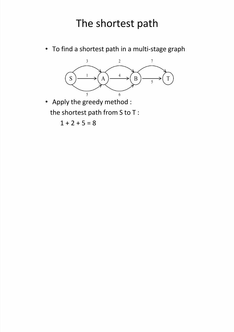
The shortest path
To find a shortest path in a multi-stage graph
Apply the greedy method :
the shortest path from S to T :
1 + 2 + 5 = 8
S A B T
3
4
5
2 7
1
5 6
5/12/2018 Dynamic Prgming & Backtracking - slidepdf.com
http://slidepdf.com/reader/full/dynamic-prgming-backtracking 7/98
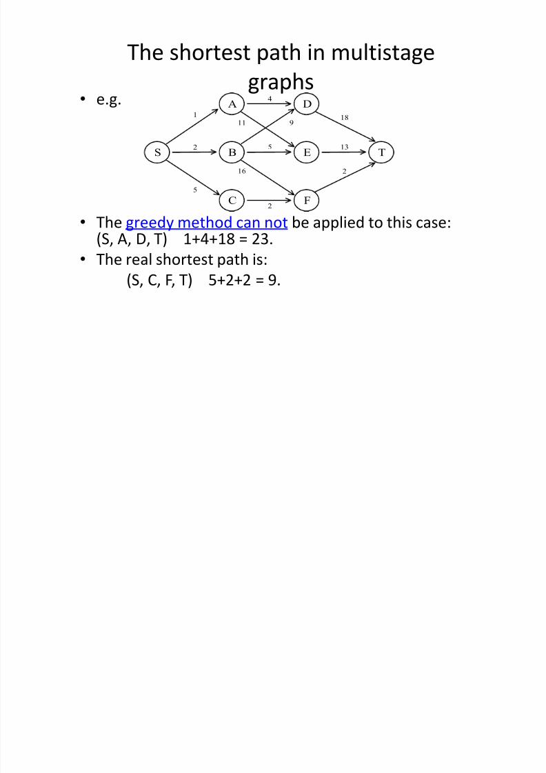
The shortest path in multistage
graphs e.g.
The greedy method can not be applied to this case:
(S, A, D, T) 1+4+18 = 23. The real shortest path is:
(S, C, F, T) 5+2+2 = 9.
S T132
B E
9
A D4
C F2
1
5
11
5
16
18
2
5/12/2018 Dynamic Prgming & Backtracking - slidepdf.com
http://slidepdf.com/reader/full/dynamic-prgming-backtracking 8/98
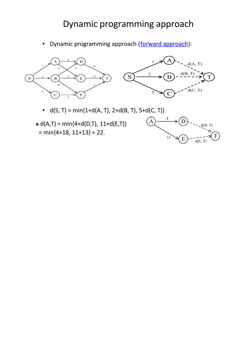
Dynamic programming approach
Dynamic programming approach (forward approach):
d(S, T) = min{1+d(A, T), 2+d(B, T), 5+d(C, T)}
S T2
B
A
C
1
5d(C, T)
d(B, T)
d(A, T)
A
T
4
E
D
11d(E, T)
d(D, T) d(A,T) = min{4+d(D,T), 11+d(E,T)}
= min{4+18, 11+13} = 22.
S T132
B E
9
A D4
C F2
1
5
11
5
16
18
2
5/12/2018 Dynamic Prgming & Backtracking - slidepdf.com
http://slidepdf.com/reader/full/dynamic-prgming-backtracking 9/98
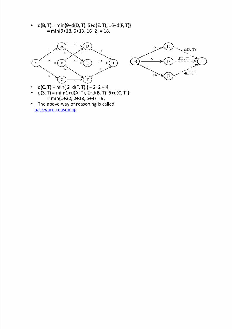
d(B, T) = min{9+d(D, T), 5+d(E, T), 16+d(F, T)}= min{9+18, 5+13, 16+2} = 18.
d(C, T) = min{ 2+d(F, T) } = 2+2 = 4 d(S, T) = min{1+d(A, T), 2+d(B, T), 5+d(C, T)}
= min{1+22, 2+18, 5+4} = 9.
The above way of reasoning is calledbackward reasoning.
B T5
E
D
F
9
16d(F, T)
d(E, T)
d(D, T)
S T132
B E
9
A D4
C F2
1
5
11
5
16
18
2
5/12/2018 Dynamic Prgming & Backtracking - slidepdf.com
http://slidepdf.com/reader/full/dynamic-prgming-backtracking 10/98
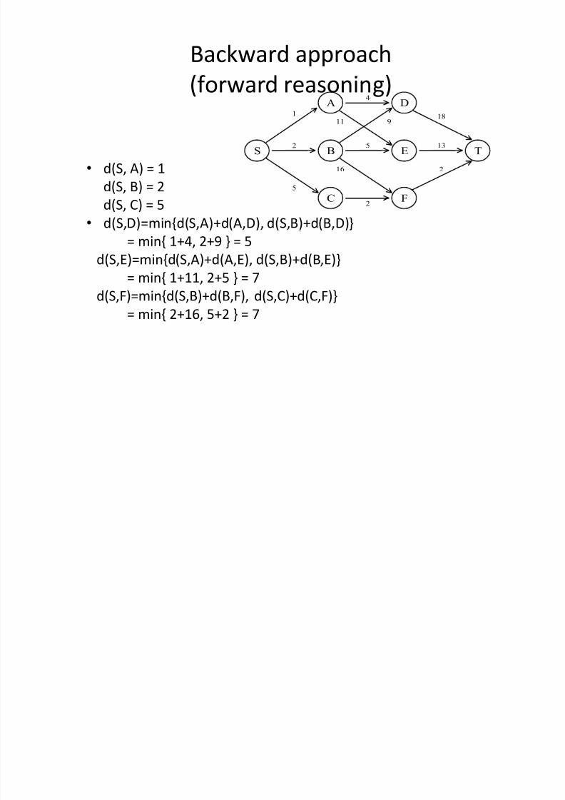
Backward approach
(forward reasoning)
d(S, A) = 1d(S, B) = 2
d(S, C) = 5
d(S,D)=min{d(S,A)+d(A,D), d(S,B)+d(B,D)}
= min{ 1+4, 2+9 } = 5
d(S,E)=min{d(S,A)+d(A,E), d(S,B)+d(B,E)}
= min{ 1+11, 2+5 } = 7
d(S,F)=min{d(S,B)+d(B,F), d(S,C)+d(C,F)}
= min{ 2+16, 5+2 } = 7
S T132
B E
9
A D4
C F2
1
5
11
5
16
18
2
5/12/2018 Dynamic Prgming & Backtracking - slidepdf.com
http://slidepdf.com/reader/full/dynamic-prgming-backtracking 11/98
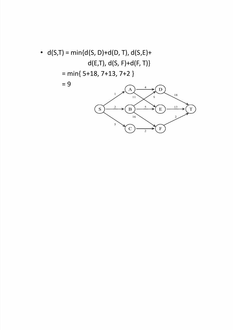
d(S,T) = min{d(S, D)+d(D, T), d(S,E)+
d(E,T), d(S, F)+d(F, T)}
= min{ 5+18, 7+13, 7+2 }
= 9
S T132
B E
9
A D4
C F2
1
5
11
5
16
18
2
5/12/2018 Dynamic Prgming & Backtracking - slidepdf.com
http://slidepdf.com/reader/full/dynamic-prgming-backtracking 12/98
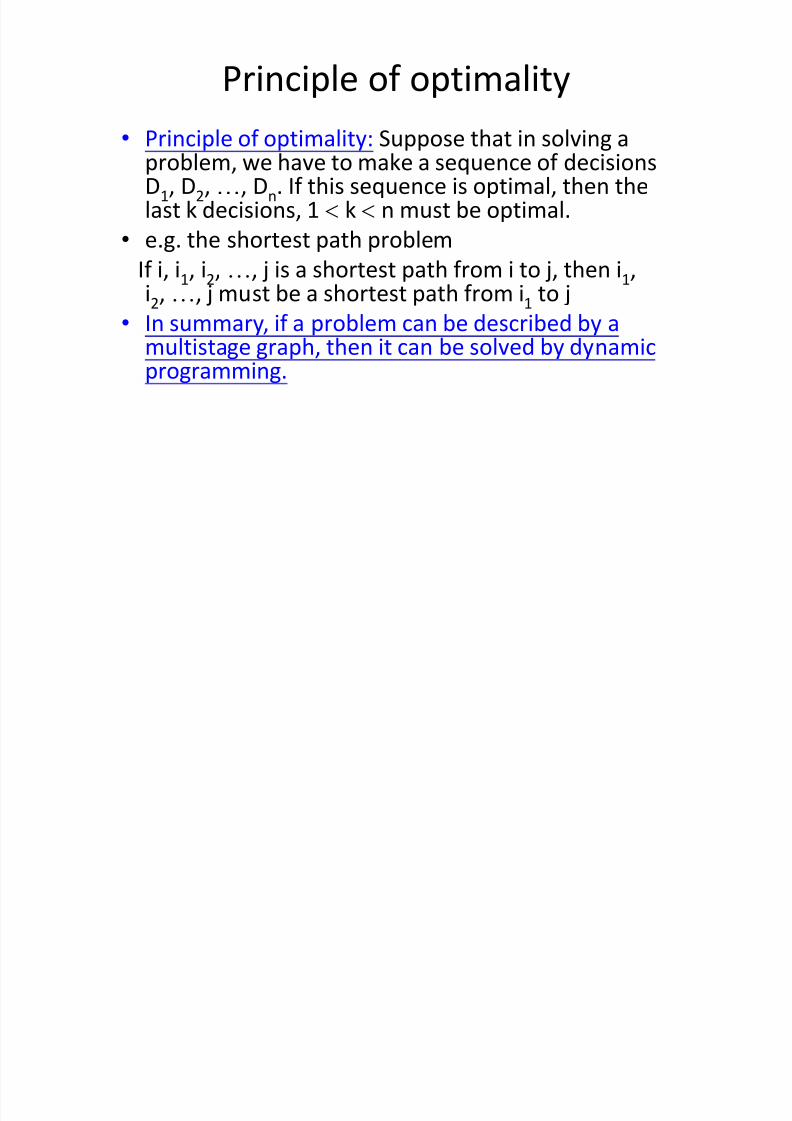
Principle of optimality
Principle of optimality: Suppose that in solving aproblem, we have to make a sequence of decisionsD1, D2, «, Dn. If this sequence is optimal, then thelast k decisions, 1 k n must be optimal.
e.g. the shortest path problemIf i, i1, i2, «, j is a shortest path from i to j, then i1,i2, «, j must be a shortest path from i1 to j
In summary, if a problem can be described by a
multistage graph, then it can be solved by dynamicprogramming.
5/12/2018 Dynamic Prgming & Backtracking - slidepdf.com
http://slidepdf.com/reader/full/dynamic-prgming-backtracking 13/98
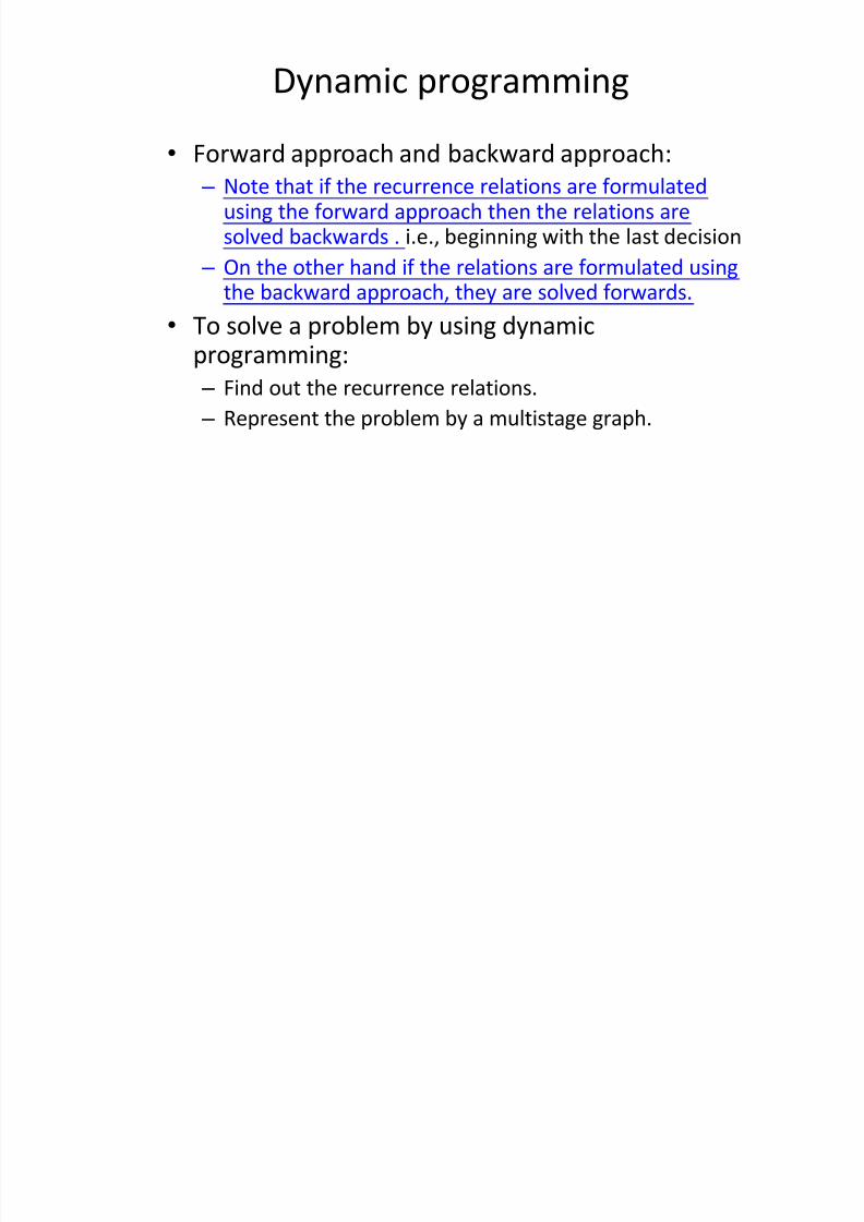
Dynamic programming
Forward approach and backward approach:
± Note that if the recurrence relations are formulatedusing the forward approach then the relations aresolved backwards . i.e., beginning with the last decision
± On the other hand if the relations are formulated usingthe backward approach, they are solved forwards.
To solve a problem by using dynamicprogramming:
± Find out the recurrence relations. ± Represent the problem by a multistage graph.

5/12/2018 Dynamic Prgming & Backtracking - slidepdf.com
http://slidepdf.com/reader/full/dynamic-prgming-backtracking 14/98
The traveling salesperson (TSP)
problem
e.g. a directed graph :
Cost matrix:
8 -14
12
3
2
44
2
56
7
104
8
39
1 2 3 41 g 2 10 52 2 g 9 g 3 4 3 g 44 6 8 7 g
5/12/2018 Dynamic Prgming & Backtracking - slidepdf.com
http://slidepdf.com/reader/full/dynamic-prgming-backtracking 15/98
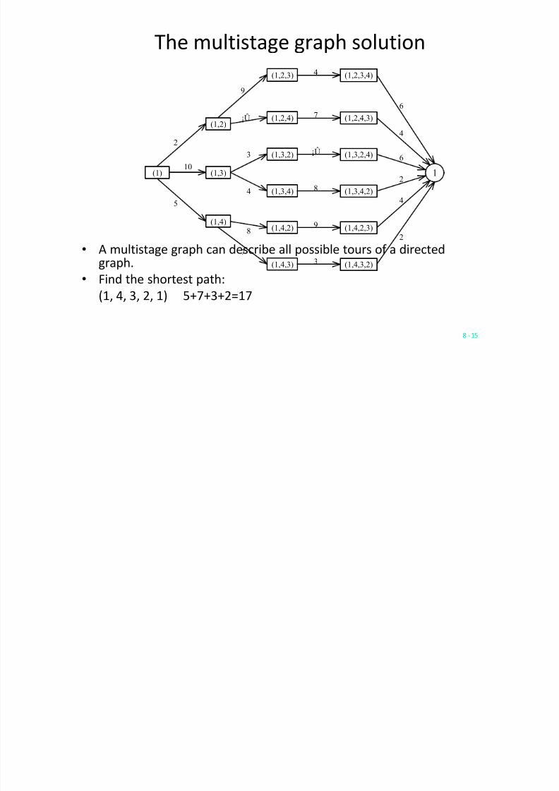
The multistage graph solution
A multistage graph can describe all possible tours of a directedgraph.
Find the shortest path:
(1, 4, 3, 2, 1) 5+7+3+2=17
8 -15
(1) (1,3)
(1,2)
(1,4)
2
5
10
(1,2,3)
(1,2,4)
(1,3,2)
(1,3,4)
(1,4,2)
(1,4,3)
9
3
4
8
7
¡Û
(1,2,3,4)
(1,2,4,3)
(1,3,2,4)
(1,3,4,2)
(1,4,2,3)
(1,4,3,2)
¡Û
4
7
8
9
3
1
4
6
6
2
4
2
5/12/2018 Dynamic Prgming & Backtracking - slidepdf.com
http://slidepdf.com/reader/full/dynamic-prgming-backtracking 16/98
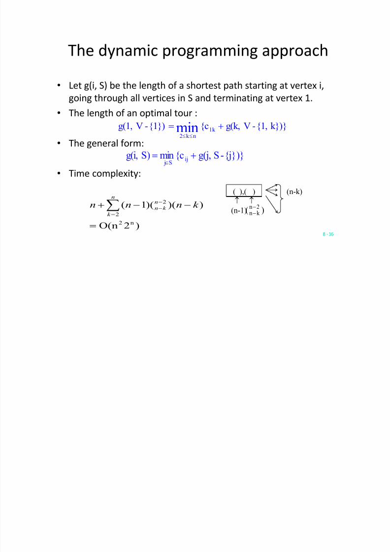
The dynamic programming approach Let g(i, S) be the length of a shortest path starting at vertex i,
going through all vertices in S and terminating at vertex 1.
The length of an optimal tour :
The general form:
Time complexity:
8 -16
k})}{1,-Vg(k ,{c{1})-Vg(1, 1k nk 2
min !ee
{j})}-Sg(j,{cminS)g(i, ijS j
!
)2O(n
))()(1(
n2
2
2
!
§!
n
k
n
k nk nnn
( ),( ) (n-k )o o
(n-1)( )n k n2
5/12/2018 Dynamic Prgming & Backtracking - slidepdf.com
http://slidepdf.com/reader/full/dynamic-prgming-backtracking 17/98
KNAPSACK PROBLEM
5/12/2018 Dynamic Prgming & Backtracking - slidepdf.com
http://slidepdf.com/reader/full/dynamic-prgming-backtracking 18/98
Knapsack Problem
Definition
Using different techniques
Brute force approach Greedy Approach
Fractional Knapsack problem

5/12/2018 Dynamic Prgming & Backtracking - slidepdf.com
http://slidepdf.com/reader/full/dynamic-prgming-backtracking 19/98
Given some items, pack the knapsack to get
the maximum total value. Each item has some
weight and some value. Total weight that we can
carry is no more than some fixed number W.So we must consider weights of items as well as
their values.
Item # Weight Value
1 1 8
2 3 6
3 5 5
Knapsack problem

5/12/2018 Dynamic Prgming & Backtracking - slidepdf.com
http://slidepdf.com/reader/full/dynamic-prgming-backtracking 20/98
Knapsack problem
There are two versions of the problem:1. 0-1 knapsack problem and
2. Fractional knapsack problem
1. Items are indivisible; you either take an item or not. Somespecial instances can be solved with dynamic programming
2. Items are divisible: you can take any fraction of an item.
Solved with a greedy algorithm
We will see this version at a later time
5/12/2018 Dynamic Prgming & Backtracking - slidepdf.com
http://slidepdf.com/reader/full/dynamic-prgming-backtracking 21/98
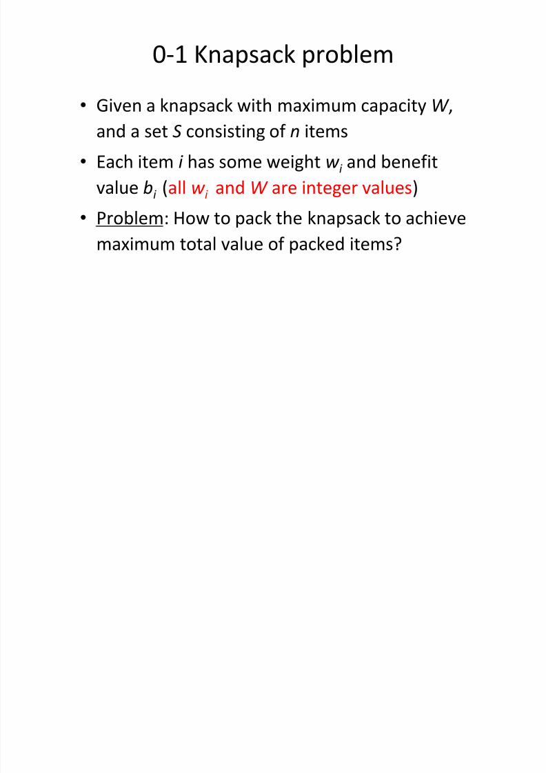
0-1 Knapsack problem
Given a knapsack with maximum capacity W ,
and a set S consisting of n items
Each item i has some weight w i and benefitvalue bi (all w i and W are integer values)
Problem: How to pack the knapsack to achieve
maximum total value of packed items?
5/12/2018 Dynamic Prgming & Backtracking - slidepdf.com
http://slidepdf.com/reader/full/dynamic-prgming-backtracking 22/98
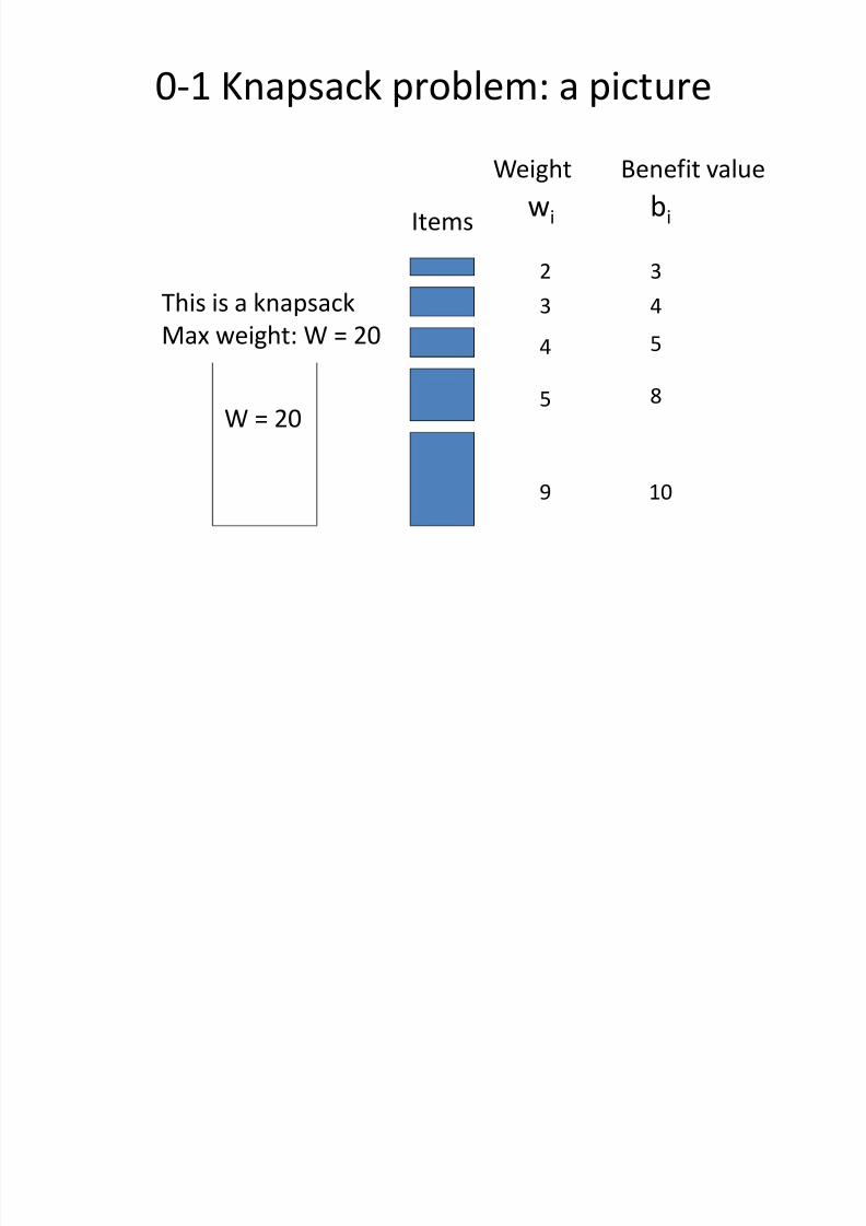
W = 20
wi bi
109
85
54
43
32
Weight Benefit value
This is a knapsack
Max weight: W = 20
Items
0-1 Knapsack problem: a picture
5/12/2018 Dynamic Prgming & Backtracking - slidepdf.com
http://slidepdf.com/reader/full/dynamic-prgming-backtracking 23/98
0-1 Knapsack problem
Problem, in other words, is to find
§§
eT i
i
T i
iW wb subject tomax
u The problem is called a 0-1 problem,
because each item must be entirely
accepted or rejected.

5/12/2018 Dynamic Prgming & Backtracking - slidepdf.com
http://slidepdf.com/reader/full/dynamic-prgming-backtracking 24/98
0-1 Knapsack problem: brute-force
approach
Lets first solve this problem with a
straightforward algorithm
Since there are n items, there are 2n
possible combinations of items.
We go through all combinations and find
the one with maximum value and with totalweight less or equal to W
Running time will be O( 2n )
5/12/2018 Dynamic Prgming & Backtracking - slidepdf.com
http://slidepdf.com/reader/full/dynamic-prgming-backtracking 25/98
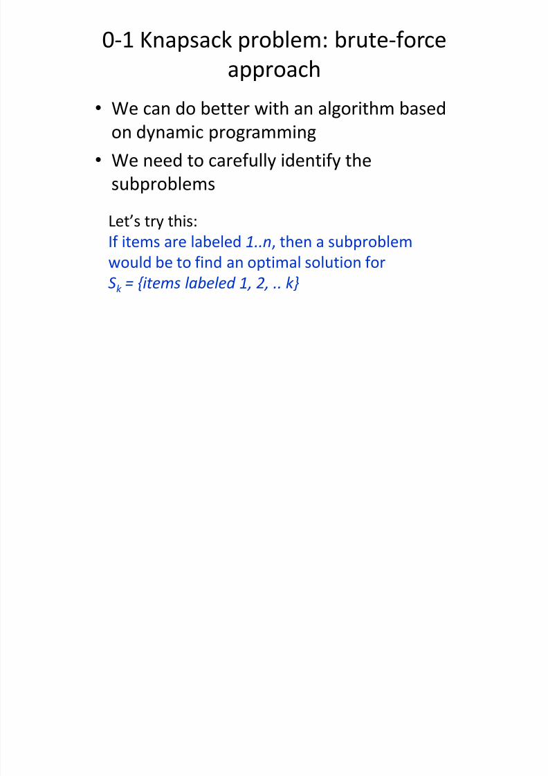
0-1 Knapsack problem: brute-force
approach
We can do better with an algorithm based
on dynamic programming
We need to carefully identify thesubproblems
Lets try this:
If items are labeled 1..n, then a subproblemwould be to find an optimal solution for
Sk = {items labeled 1, 2 , .. k}
5/12/2018 Dynamic Prgming & Backtracking - slidepdf.com
http://slidepdf.com/reader/full/dynamic-prgming-backtracking 26/98
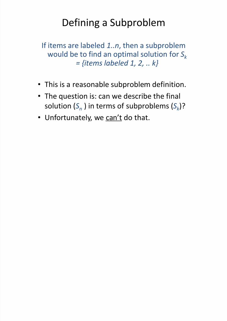
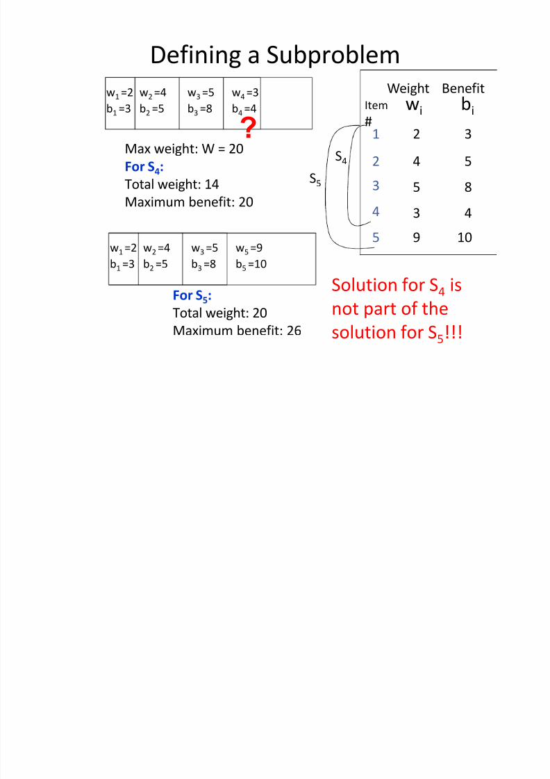
Defining a Subproblem
If items are labeled 1..n, then a subproblemwould be to find an optimal solution for Sk
= {items labeled 1, 2 , .. k}
This is a reasonable subproblem definition.
The question is: can we describe the final
solution (Sn ) in terms of subproblems (Sk )?
Unfortunately, we cant do that.
5/12/2018 Dynamic Prgming & Backtracking - slidepdf.com
http://slidepdf.com/reader/full/dynamic-prgming-backtracking 27/98
Max weight: W = 20
For S4:Total weight: 14
Maximum benefit: 20
w1 =2
b1 =3
w2 =4
b2 =5
w3 =5
b3 =8
w4 =3
b4 =4 wi bi
10
8554
43
32
Weight Benefit
9
Item
#
4
32
1
5
S4
S5
w1 =2b1 =3
w2 =4b2 =5
w3 =5b3 =8
w5 =9b5 =10
For S5:
Total weight: 20
Maximum benefit: 26
Solution for S4 is
not part of the
solution for S5!!!
?
Defining a Subproblem
5/12/2018 Dynamic Prgming & Backtracking - slidepdf.com
http://slidepdf.com/reader/full/dynamic-prgming-backtracking 28/98
Defining a Subproblem (continued)
As we have seen, the solution for S4 is not part of the solution for S5
So our definition of a subproblem is flawed and
we need another one! Lets add another parameter: w , which will
represent the maximum weight for each subsetof items
The subproblem then will be to compute V[ k ,w] , i .e., to find an optimal solution for Sk = {itemslabeled 1, 2 , .. k} in a k napsack of size w
5/12/2018 Dynamic Prgming & Backtracking - slidepdf.com
http://slidepdf.com/reader/full/dynamic-prgming-backtracking 29/98
Recursive Formula for subproblems
The subproblem then will be to compute
V[ k ,w] , i .e., to find an optimal solution for Sk =
{items labeled 1, 2 , .. k} in a k napsack of size w
Assuming knowing V[i, j], where i=0,1, 2, k-1,
j=0,1,2, w, how to derive V[k,w]?
5/12/2018 Dynamic Prgming & Backtracking - slidepdf.com
http://slidepdf.com/reader/full/dynamic-prgming-backtracking 30/98
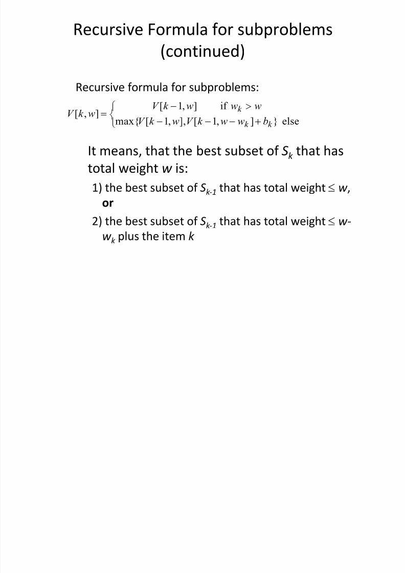
Recursive Formula for subproblems
(continued)
It means, that the best subset of Sk that has
total weight w is:
1) the best subset of Sk -1 that has total weight e w ,
or
2) the best subset of Sk -1 that has total weight e w -
w k plus the item k
°¯®
"!
else }],1[],,1[max{
if ],1[],[
k k
k
bwwk V wk V
wwwk V wk V
Recursive formula for subproblems:
5/12/2018 Dynamic Prgming & Backtracking - slidepdf.com
http://slidepdf.com/reader/full/dynamic-prgming-backtracking 31/98
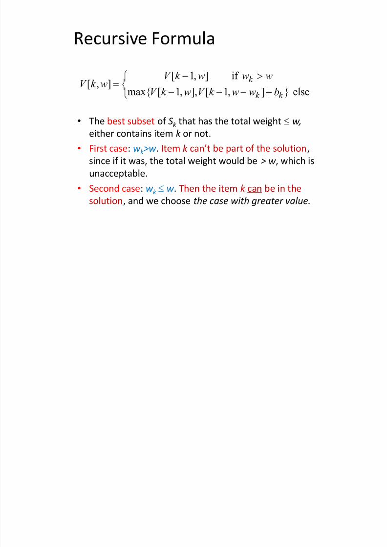
Recursive Formula
The best subset of Sk that has the total weight e w ,
either contains item k or not.
First case: w k >w . Item k cant be part of the solution,
since if it was, the total weight would be > w , which is
unacceptable. Second case: w k e w . Then the item k can be in the
solution, and we choose the case with greater value.
°¯®
"!
else }],1[],,1[max{
if ],1[],[
k k
k
bwwk V wk V
wwwk V wk V

5/12/2018 Dynamic Prgming & Backtracking - slidepdf.com
http://slidepdf.com/reader/full/dynamic-prgming-backtracking 32/98
0/1 Knapsack Problem
We are given a knapsack of capacity c and a set of n objects numbered1,2 ,,n. Each object i has weight w i and profit pi .
Let v = [ v 1 , v 2 ,, v n ] be a solution vector in which v i = 0 if object i is not inthe knapsack, and v i = 1 if it is in the knapsack.
The goal is to find a subset of objects to put into the knapsack so that
(that is, the objects fit into the knapsack) and
is maximized (that is, the profit is maximized).
5/12/2018 Dynamic Prgming & Backtracking - slidepdf.com
http://slidepdf.com/reader/full/dynamic-prgming-backtracking 33/98
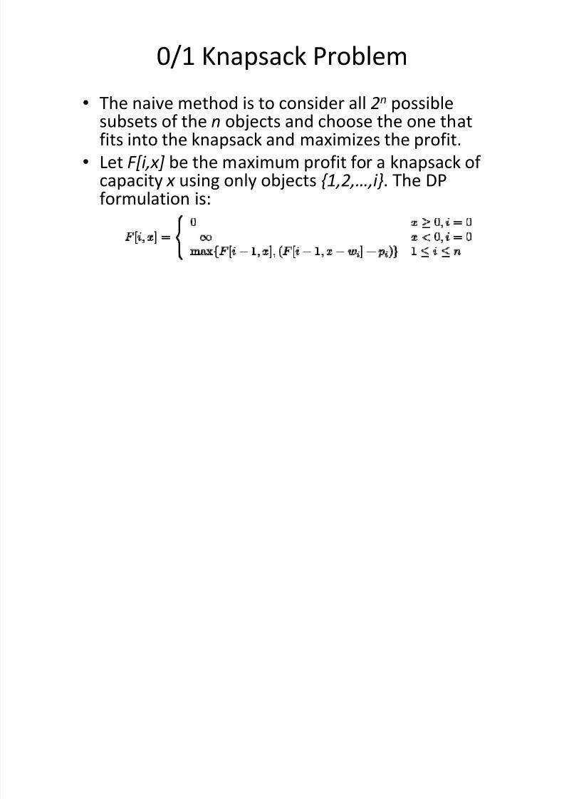
0/1 Knapsack Problem
The naive method is to consider all 2n possiblesubsets of the n objects and choose the one thatfits into the knapsack and maximizes the profit.
Let
F [ i ,x ] be the maximum profit for a knapsack of capacity x using only objects { 1,2 ,,i }. The DP
formulation is:
5/12/2018 Dynamic Prgming & Backtracking - slidepdf.com
http://slidepdf.com/reader/full/dynamic-prgming-backtracking 34/98
0/1 Knapsack Problem
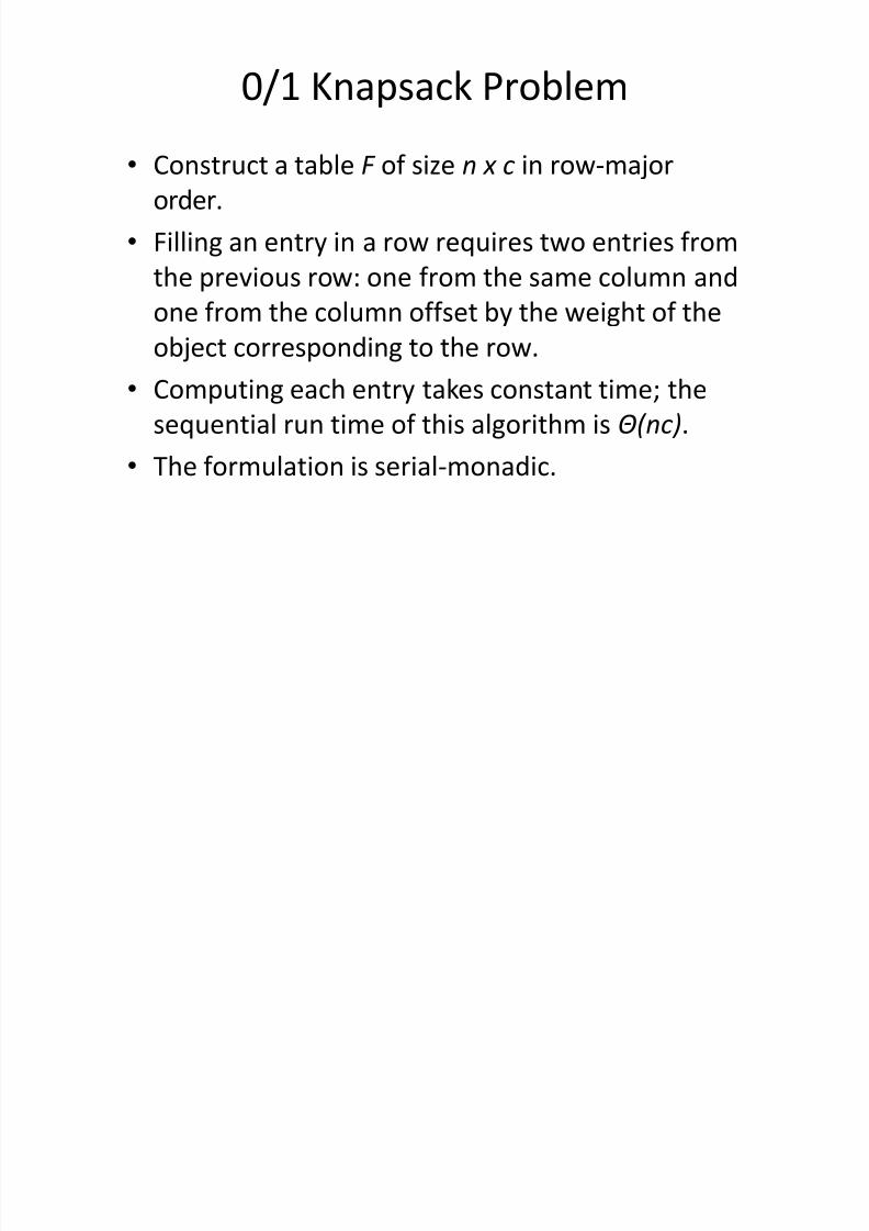
Construct a table F of size n x c in row-major
order.
Filling an entry in a row requires two entries from
the previous row: one from the same column and
one from the column offset by the weight of the
object corresponding to the row.
Computing each entry takes constant time; thesequential run time of this algorithm is ( nc).
The formulation is serial-monadic.
5/12/2018 Dynamic Prgming & Backtracking - slidepdf.com
http://slidepdf.com/reader/full/dynamic-prgming-backtracking 35/98
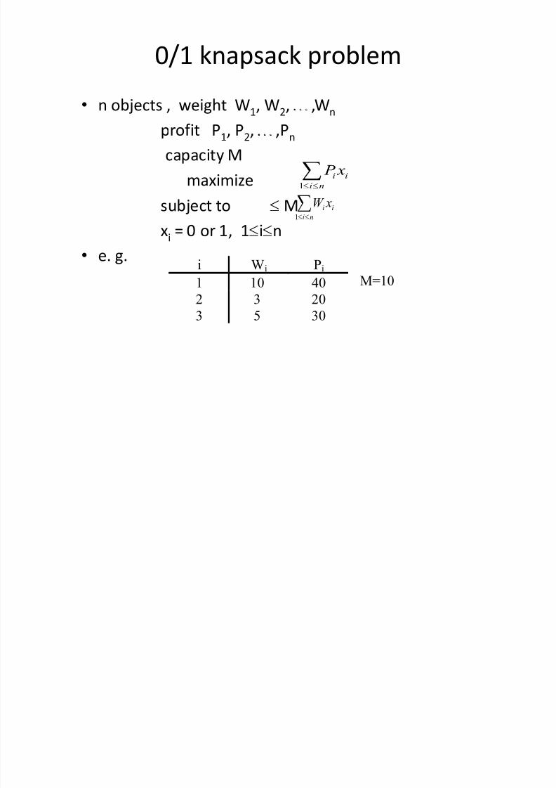
0/1 knapsack problem
n objects , weight W1, W2,~,Wn
profit P1, P2,~,Pn
capacity M
maximize
subject to e M
xi = 0 or 1, 1eien
e. g.
§ee ni
ii x P 1
§ee ni
ii xW
1
i Wi Pi 1 10 402 3 203 5 30
M=10
5/12/2018 Dynamic Prgming & Backtracking - slidepdf.com
http://slidepdf.com/reader/full/dynamic-prgming-backtracking 36/98
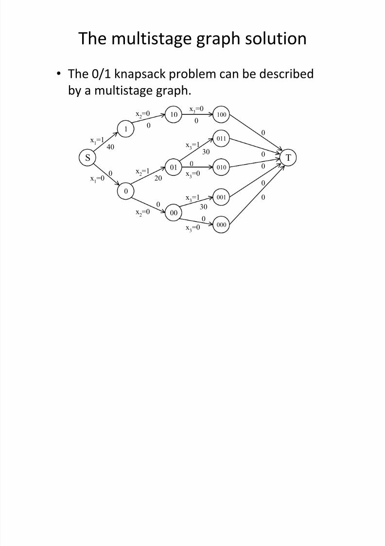
The multistage graph solution
The 0/1 knapsack problem can be described
by a multistage graph.
S T
0
1 0
10
00
01
100
010
011
000
001
0
0
0
0
00
40
0 20
0
30
0
0
30
x1=1
x1=0
x2=0
x2=1
x2=0
x3=0
x3=1
x3=0
x3=1
x3=0

5/12/2018 Dynamic Prgming & Backtracking - slidepdf.com
http://slidepdf.com/reader/full/dynamic-prgming-backtracking 37/98
The dynamic programming approach
The longest path represents the optimal solution:
x1=0, x2=1, x3=1
= 20+30 = 50
Let f i(Q) be the value of an optimal solution to
objects 1,2,3,«,i with capacity Q.
f i(Q) = max{ f i-1(Q), f i-1(Q-Wi)+Pi }
The optimal solution is f n(M).
§ ii x P

5/12/2018 Dynamic Prgming & Backtracking - slidepdf.com
http://slidepdf.com/reader/full/dynamic-prgming-backtracking 38/98
FLOW SHOP SCHEDULING
5/12/2018 Dynamic Prgming & Backtracking - slidepdf.com
http://slidepdf.com/reader/full/dynamic-prgming-backtracking 39/98
Flow shop scheduling
Definition
Scheduling classification
Simple Flow shop problem Flexible Flow shop problem
Johnsons rule
5/12/2018 Dynamic Prgming & Backtracking - slidepdf.com
http://slidepdf.com/reader/full/dynamic-prgming-backtracking 40/98
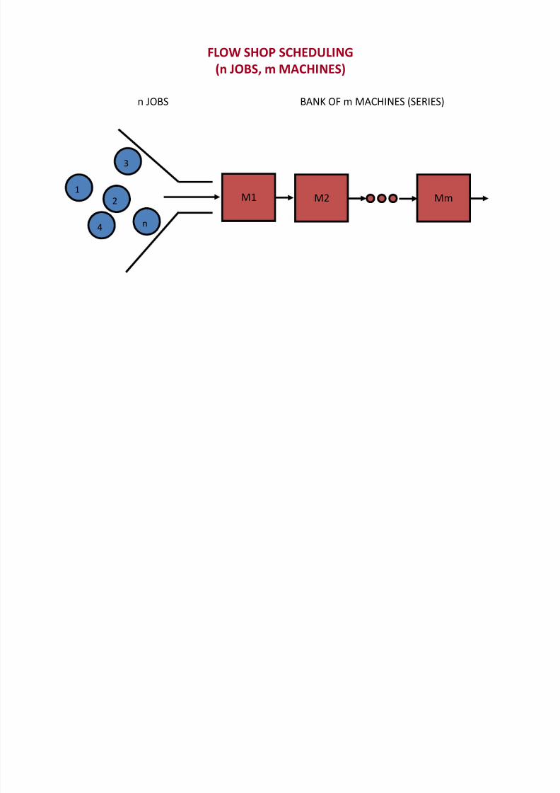
FLOW SHOP SCHEDULING
(n JOBS, m MACHINES)
n JOBS BANK OF m MACHINES (SERIES)
1
2
3
4 n
M1 M2 Mm
5/12/2018 Dynamic Prgming & Backtracking - slidepdf.com
http://slidepdf.com/reader/full/dynamic-prgming-backtracking 41/98
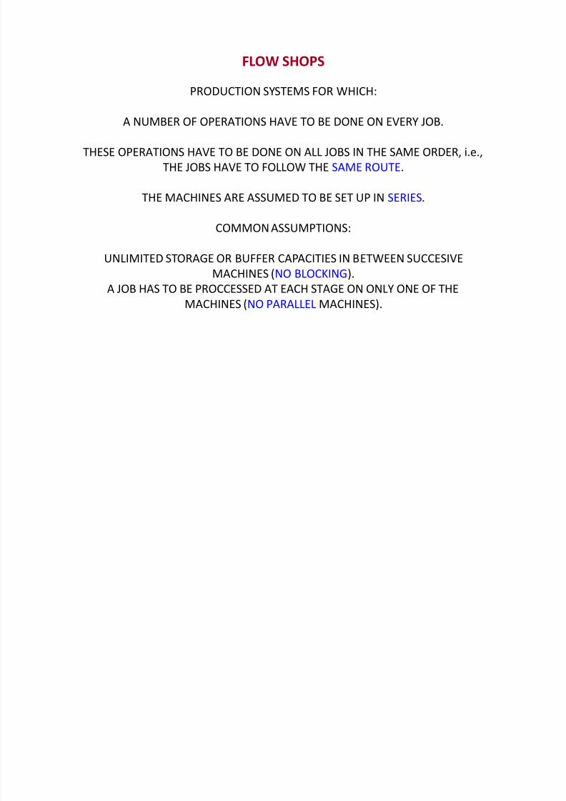
FLOW SHOPS
PRODUCTION SYSTEMS FOR WHICH:
A NUMBER OF OPERATIONS HAVE TO BE DONE ON EVERY JOB.
THESE OPERATIONS HAVE TO BE DONE ON ALL JOBS IN THE SAME ORDER, i.e.,
THE JOBS HAVE TO FOLLOW THE SAME ROUTE.
THE MACHINES ARE ASSUMED TO BE SET UP IN SERIES.
COMMON ASSUMPTIONS:
UNLIMITED STORAGE OR BUFFER CAPACITIES IN BETWEEN SUCCESIVEMACHINES (NO BLOCKING).
A JOB HAS TO BE PROCCESSED AT EACH STAGE ON ONLY ONE OF THE
MACHINES (NO PARALLEL MACHINES).
5/12/2018 Dynamic Prgming & Backtracking - slidepdf.com
http://slidepdf.com/reader/full/dynamic-prgming-backtracking 42/98
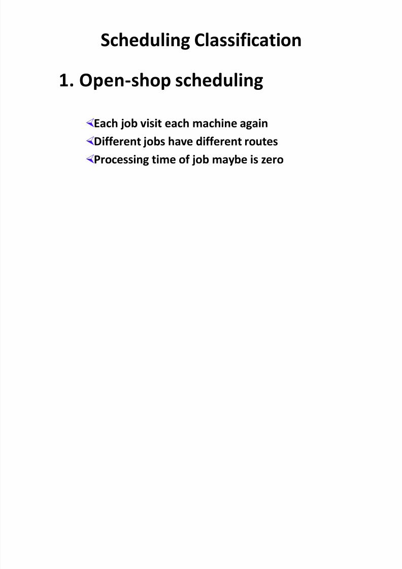
Scheduling Classification
1. Open-shop scheduling
Each job visit each machine again Different jobs have different routes
Processing time of job maybe is zero
5/12/2018 Dynamic Prgming & Backtracking - slidepdf.com
http://slidepdf.com/reader/full/dynamic-prgming-backtracking 43/98
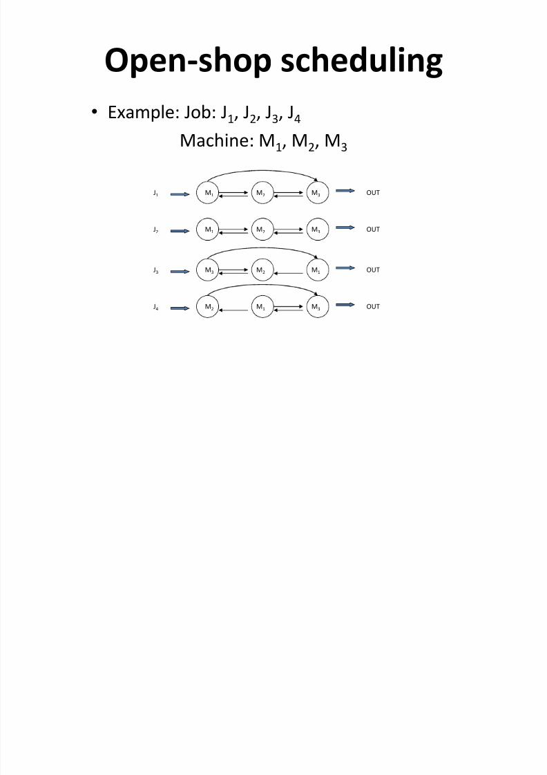
Open-shop scheduling
Example: Job: J1, J2, J3, J4
Machine: M1, M2, M3
M1 M2 M3J1 OUT
M1 M2 M3J2 OUT
M3 M2 M1J3 OUT
M2 M1 M3J4 OUT
5/12/2018 Dynamic Prgming & Backtracking - slidepdf.com
http://slidepdf.com/reader/full/dynamic-prgming-backtracking 44/98
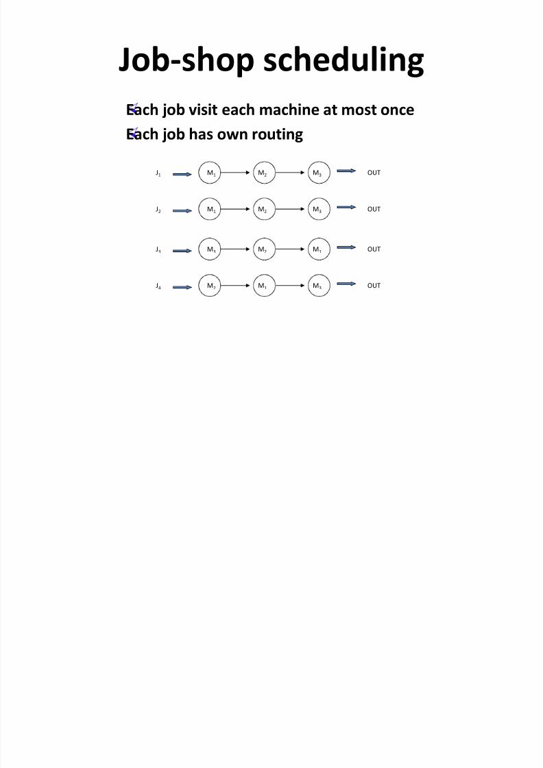
Job-shop scheduling
Each job visit each machine at most once
Each job has own routing
M1 M2 M3J1 OUT
M1 M2 M3J2 OUT
M3 M2 M1J3 OUT
M2 M1 M3J4 OUT
5/12/2018 Dynamic Prgming & Backtracking - slidepdf.com
http://slidepdf.com/reader/full/dynamic-prgming-backtracking 45/98
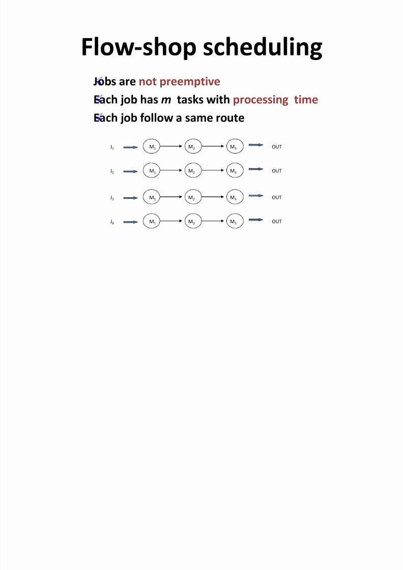
Flow-shop scheduling Jobs are not preemptive
Each job has m tasks with processing time
Each j
ob f o
llow
a same ro
ute
M1 M2 M3J1 OUT
M1 M2 M3J2 OUT
M1 M2 M3J3 OUT
M1 M2 M3J4 OUT
5/12/2018 Dynamic Prgming & Backtracking - slidepdf.com
http://slidepdf.com/reader/full/dynamic-prgming-backtracking 46/98
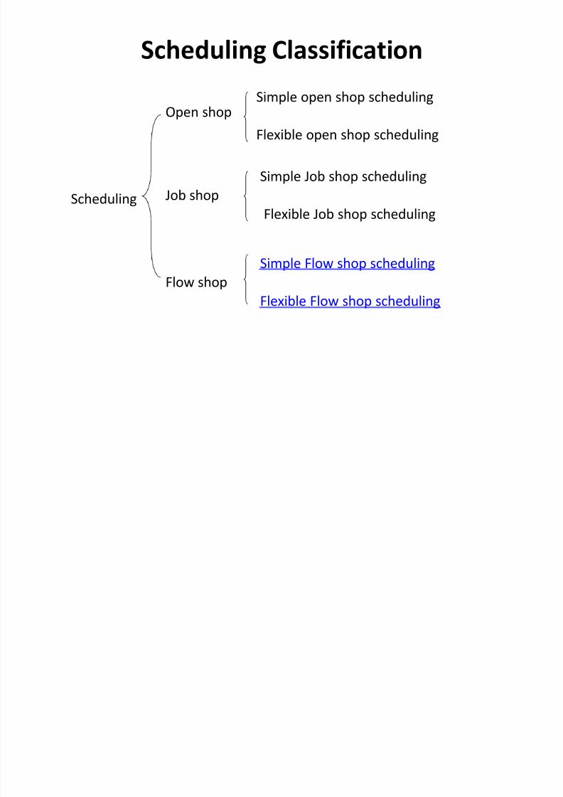
Scheduling Classification
Scheduling
Open shop
Job shop
Flow shop
Simple open shop scheduling
Flexible open shop scheduling
Simple Job shop scheduling
Flexible Job shop scheduling
Simple Flow shop scheduling
Flexible Flow shop scheduling

5/12/2018 Dynamic Prgming & Backtracking - slidepdf.com
http://slidepdf.com/reader/full/dynamic-prgming-backtracking 47/98
(5, 3)
(4, 4)
C ar -1
C ar -2 paintingP2
degreasingP1
Each machine center has one machineEx: A car painting factory
Center 1
Center 2
5 9
8 13
The final completion time=13
Simple Flow Shop Problem
5/12/2018 Dynamic Prgming & Backtracking - slidepdf.com
http://slidepdf.com/reader/full/dynamic-prgming-backtracking 48/98
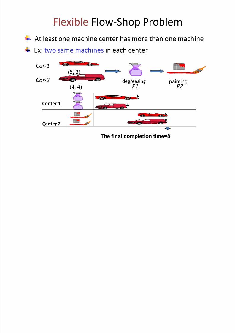
At least one machine center has more than one machine
Ex: two same machines in each center
Flexible Flow-Shop Problem
The final completion time=8
Center 2
Center 1
8
84
5
(5, 3)
(4, 4)
C ar -1
C ar -2 paintingP2
degreasingP1
5/12/2018 Dynamic Prgming & Backtracking - slidepdf.com
http://slidepdf.com/reader/full/dynamic-prgming-backtracking 49/98
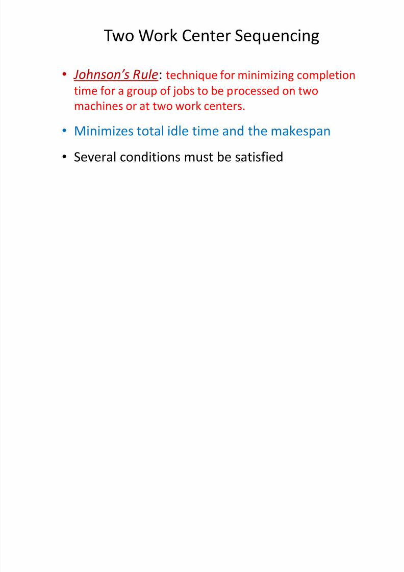
Two Work Center Sequencing
Johnsons Rule: technique for minimizing completion
time for a group of jobs to be processed on two
machines or at two work centers.
Minimizes total idle time and the makespan
Several conditions must be satisfied

5/12/2018 Dynamic Prgming & Backtracking - slidepdf.com
http://slidepdf.com/reader/full/dynamic-prgming-backtracking 50/98
Johnsons Rule Conditions
Job time must be known and constant
Job times must be independent of sequence
Jobs must follow same two-step sequence
Job priorities cannot be used
All units must be completed at the first
work center before moving to the second
5/12/2018 Dynamic Prgming & Backtracking - slidepdf.com
http://slidepdf.com/reader/full/dynamic-prgming-backtracking 51/98
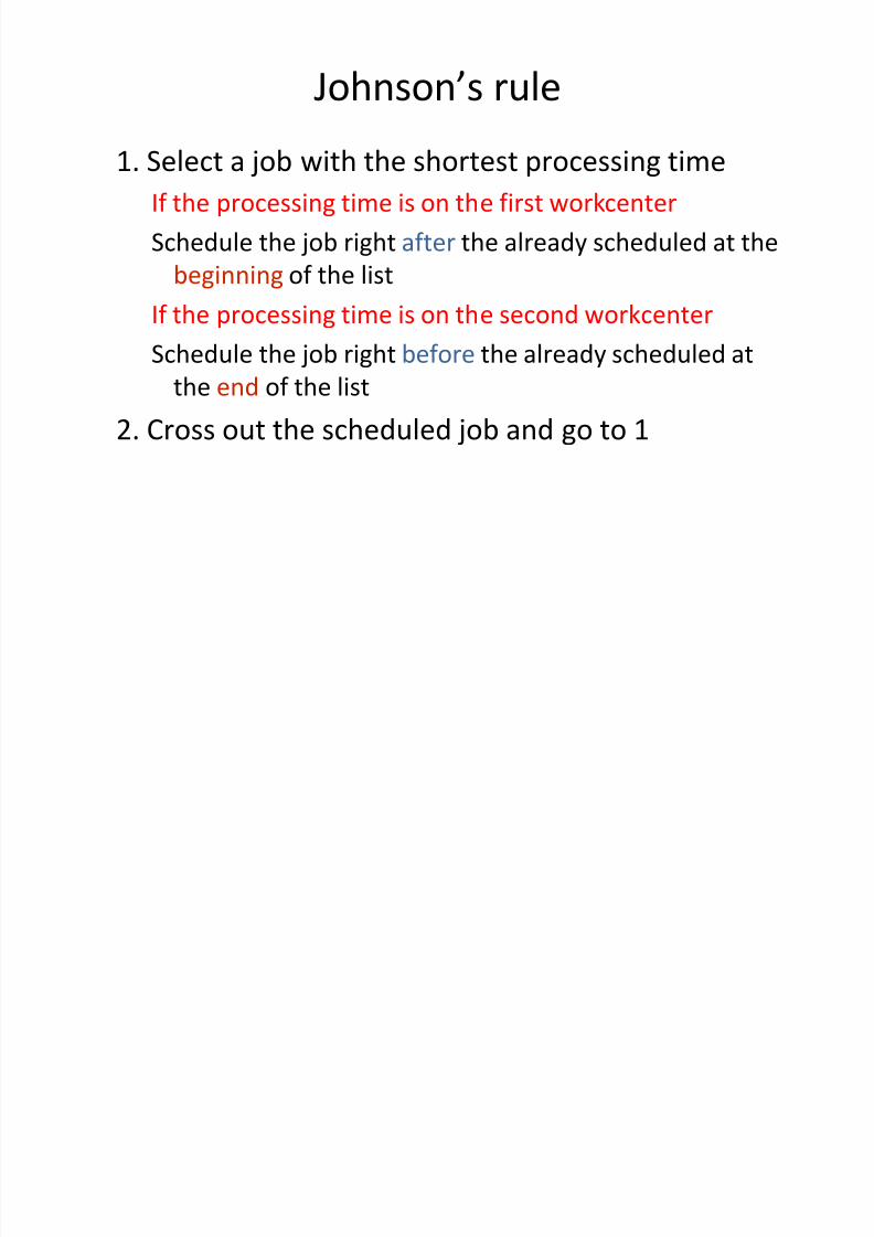
Johnsons rule
1. Select a job with the shortest processing time
If the processing time is on the first workcenter
Schedule the job right after the already scheduled at the
beginning of the list
If the processing time is on the second workcenter
Schedule the job right before the already scheduled at
the end of the list2. Cross out the scheduled job and go to 1
5/12/2018 Dynamic Prgming & Backtracking - slidepdf.com
http://slidepdf.com/reader/full/dynamic-prgming-backtracking 52/98
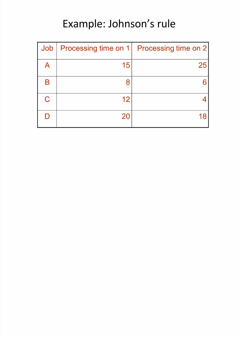
Example: Johnsons rule
Job Processing time on 1 Processing time on 2
A 15 25
B 8 6
C 12 4
D 20 18
The sequence that minimizes the
5/12/2018 Dynamic Prgming & Backtracking - slidepdf.com
http://slidepdf.com/reader/full/dynamic-prgming-backtracking 53/98
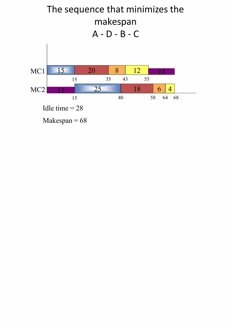
The sequence that minimizes the
makespan
A - D - B - C
15
25
20
18
8
6
12
415
15 35
40
43
58
55
64 6815
13
Idle time = 28
Mak espan = 68
MC1
MC2
5/12/2018 Dynamic Prgming & Backtracking - slidepdf.com
http://slidepdf.com/reader/full/dynamic-prgming-backtracking 54/98
Sequence dependent set up times
Set up is basically changing the work center
configuration from the existing to the new
Set up depends on the existing configuration Set up time of an operation depends on
previous operation done on the same work
center Which sequence minimizes total set up time?
There are too many sequences!
5/12/2018 Dynamic Prgming & Backtracking - slidepdf.com
http://slidepdf.com/reader/full/dynamic-prgming-backtracking 55/98
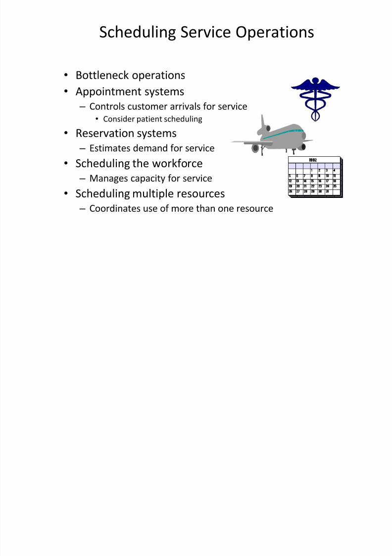
Scheduling Service Operations
Bottleneck operations
Appointment systems
± Controls customer arrivals for service
Consider patient scheduling
Reservation systems
± Estimates demand for service
Scheduling the workforce
± Manages capacity for service Scheduling multiple resources
± Coordinates use of more than one resource

5/12/2018 Dynamic Prgming & Backtracking - slidepdf.com
http://slidepdf.com/reader/full/dynamic-prgming-backtracking 56/98
N-Q UEEN PROBLEM
5/12/2018 Dynamic Prgming & Backtracking - slidepdf.com
http://slidepdf.com/reader/full/dynamic-prgming-backtracking 57/98
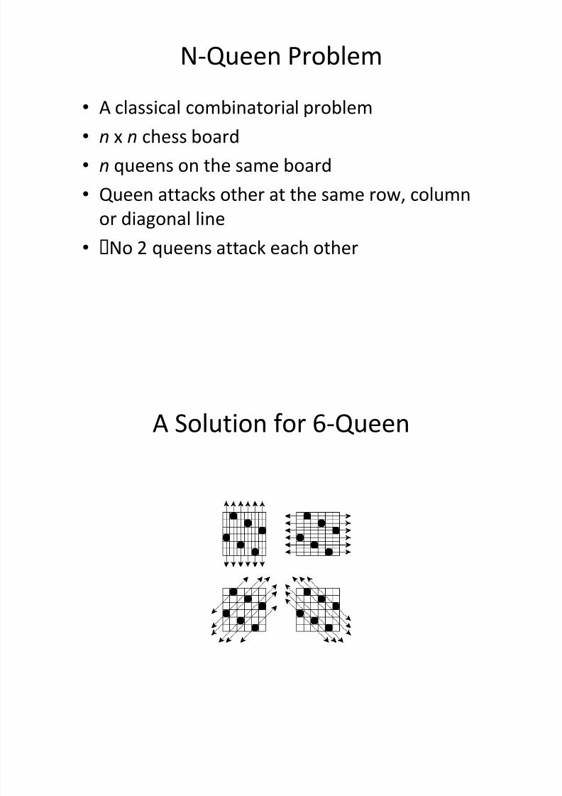
N-Queen Problem
A classical combinatorial problem
n x n chess board
n queens on the same board
Queen attacks other at the same row, column
or diagonal line
No 2 queens attack each other

5/12/2018 Dynamic Prgming & Backtracking - slidepdf.com
http://slidepdf.com/reader/full/dynamic-prgming-backtracking 58/98
A Solution for 6-Queen
5/12/2018 Dynamic Prgming & Backtracking - slidepdf.com
http://slidepdf.com/reader/full/dynamic-prgming-backtracking 59/98
Previous Works
Analytical solution
± Direct computation, very fast
± Generate only a very restricted class of solutions
Backtracking Search
± Generate all possible solutions
± Exponential time complexity
± Can only solve for n<100
5/12/2018 Dynamic Prgming & Backtracking - slidepdf.com
http://slidepdf.com/reader/full/dynamic-prgming-backtracking 60/98
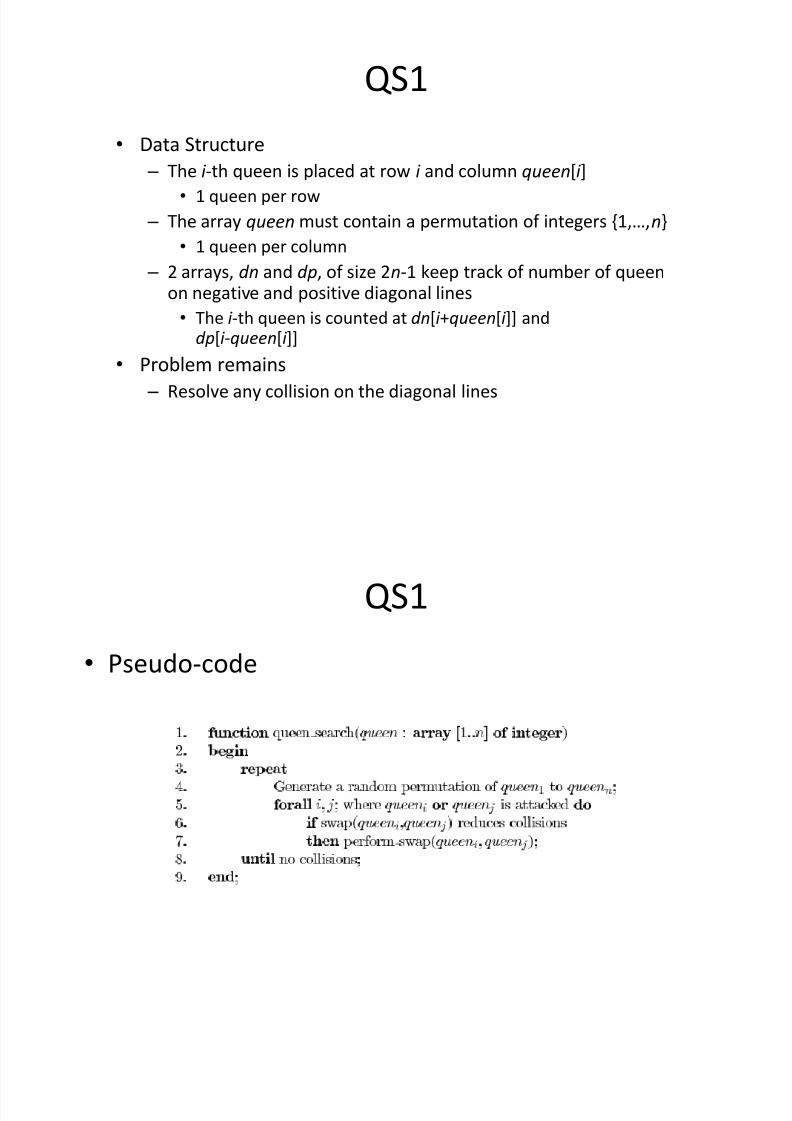
QS1
Data Structure
± The i -th queen is placed at row i and column queen[i ]
1 queen per row
± The array queen must contain a permutation of integers {1,,n}
1 queen per column
± 2 arrays, dn and dp, of size 2n-1 keep track of number of queenon negative and positive diagonal lines
The i -th queen is counted at dn[i +queen[i ]] anddp[i -queen[i ]]
Problem remains ± Resolve any collision on the diagonal lines

5/12/2018 Dynamic Prgming & Backtracking - slidepdf.com
http://slidepdf.com/reader/full/dynamic-prgming-backtracking 61/98
QS1
Pseudo-code
5/12/2018 Dynamic Prgming & Backtracking - slidepdf.com
http://slidepdf.com/reader/full/dynamic-prgming-backtracking 62/98
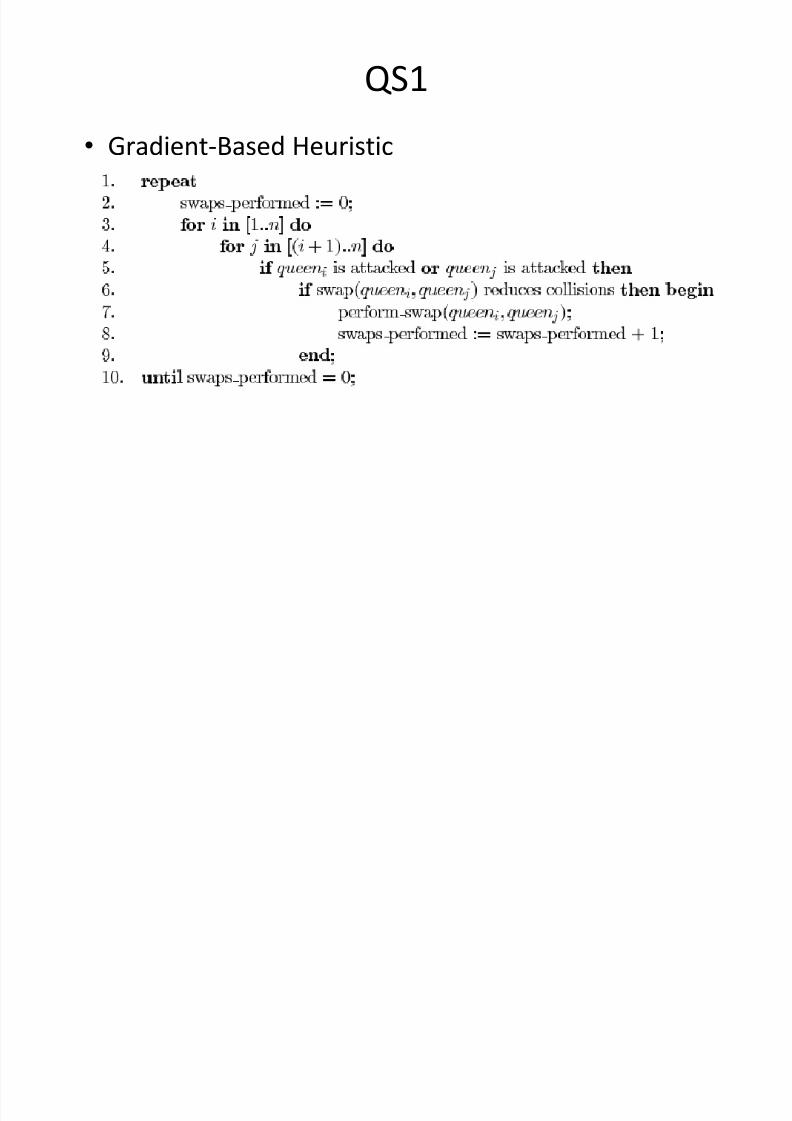
QS1
Gradient-Based Heuristic
5/12/2018 Dynamic Prgming & Backtracking - slidepdf.com
http://slidepdf.com/reader/full/dynamic-prgming-backtracking 63/98
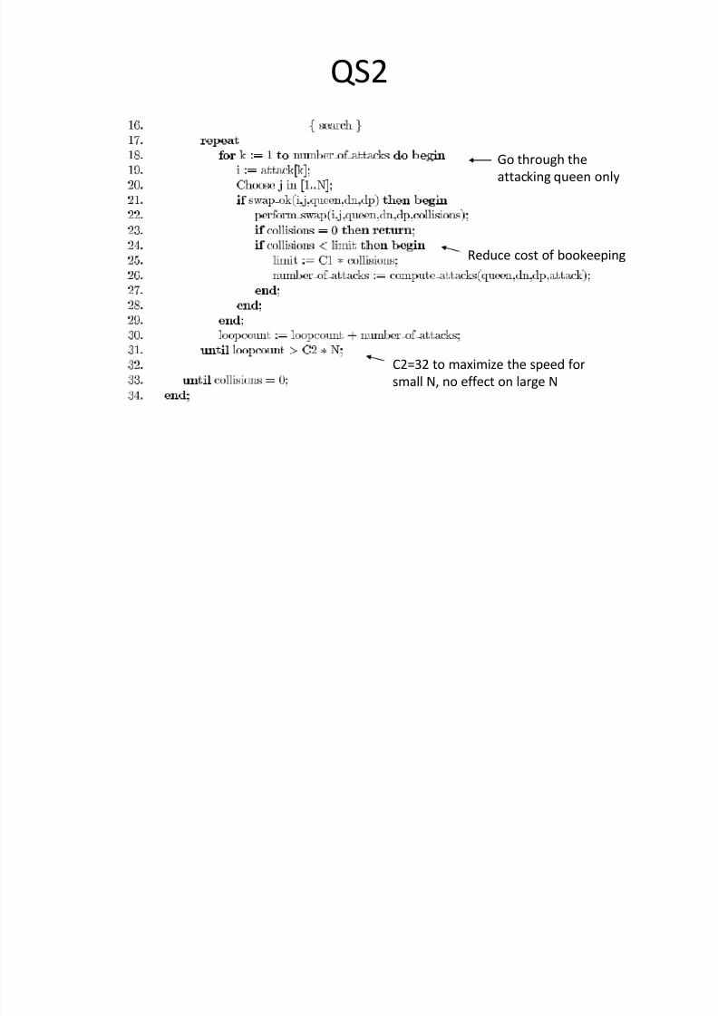
QS2
Data Structure
± Queen placement same as QS1
± An array attack is maintained
Store the row indexes of queens that are under attack
5/12/2018 Dynamic Prgming & Backtracking - slidepdf.com
http://slidepdf.com/reader/full/dynamic-prgming-backtracking 64/98
QS2
Pseudo-code
5/12/2018 Dynamic Prgming & Backtracking - slidepdf.com
http://slidepdf.com/reader/full/dynamic-prgming-backtracking 65/98
QS2
Reduce cost of bookeeping
Go through the
attacking queen only
C2=32 to maximize the speed for
small N, no effect on large N
5/12/2018 Dynamic Prgming & Backtracking - slidepdf.com
http://slidepdf.com/reader/full/dynamic-prgming-backtracking 66/98
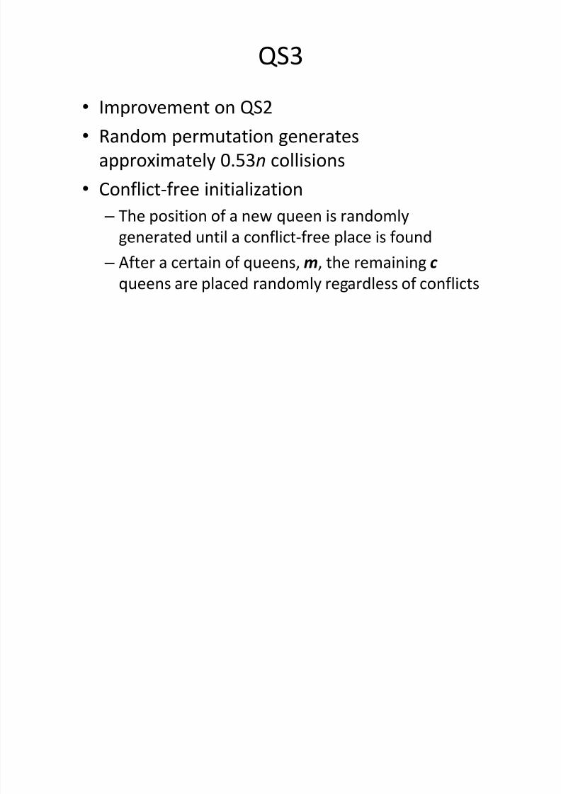
QS3
Improvement on QS2
Random permutation generates
approximately 0.53n collisions
Conflict-free initialization
± The position of a new queen is randomly
generated until a conflict-free place is found
± After a certain of queens, m, the remaining c
queens are placed randomly regardless of conflicts
5/12/2018 Dynamic Prgming & Backtracking - slidepdf.com
http://slidepdf.com/reader/full/dynamic-prgming-backtracking 67/98
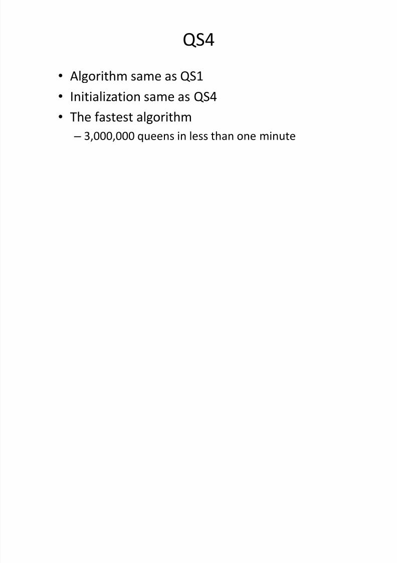
QS4
Algorithm same as QS1
Initialization same as QS4
The fastest algorithm ± 3,000,000 queens in less than one minute
5/12/2018 Dynamic Prgming & Backtracking - slidepdf.com
http://slidepdf.com/reader/full/dynamic-prgming-backtracking 68/98
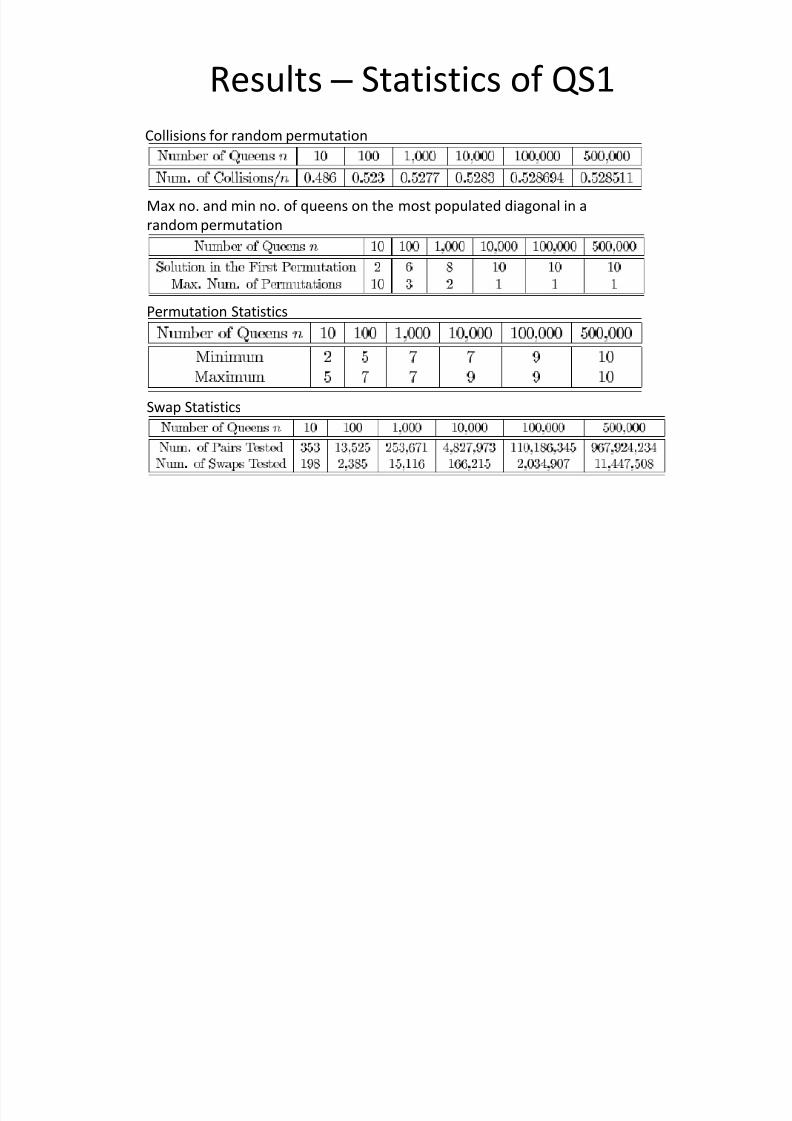
Results ± Statistics of QS1
Collisions for random permutation
Max no. and min no. of queens on the most populated diagonal in a
random permutation
Permutation Statistics
Swap Statistics
5/12/2018 Dynamic Prgming & Backtracking - slidepdf.com
http://slidepdf.com/reader/full/dynamic-prgming-backtracking 69/98
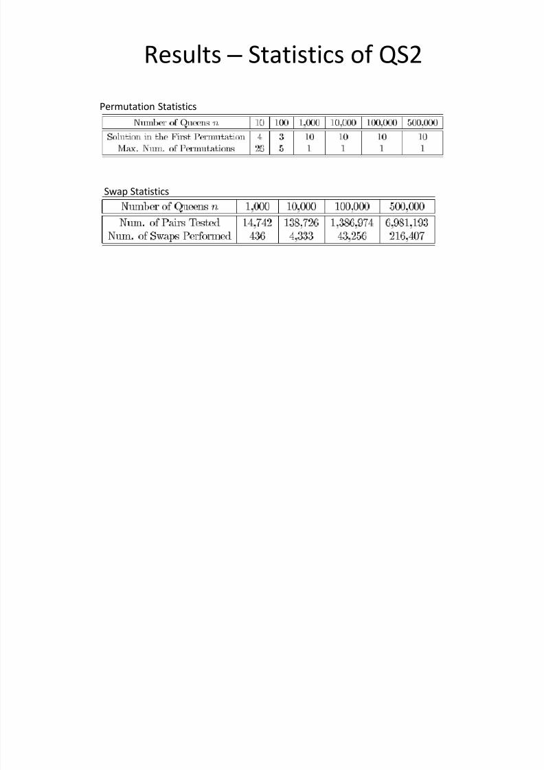
Results ± Statistics of QS2
Permutation Statistics
Swap Statistics

5/12/2018 Dynamic Prgming & Backtracking - slidepdf.com
http://slidepdf.com/reader/full/dynamic-prgming-backtracking 70/98
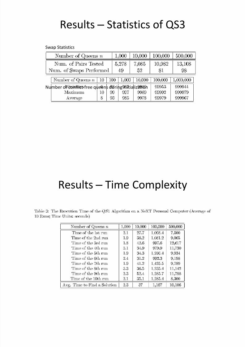
Results ± Statistics of QS3
Swap Statistics
Number of conflict-free queens during initialization

5/12/2018 Dynamic Prgming & Backtracking - slidepdf.com
http://slidepdf.com/reader/full/dynamic-prgming-backtracking 71/98
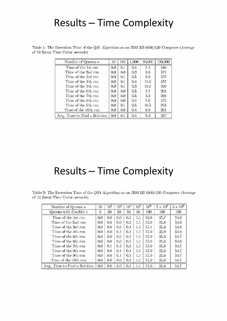
Results ± Time Complexity
5/12/2018 Dynamic Prgming & Backtracking - slidepdf.com
http://slidepdf.com/reader/full/dynamic-prgming-backtracking 72/98
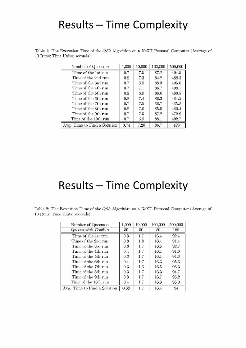
Results ± Time Complexity
5/12/2018 Dynamic Prgming & Backtracking - slidepdf.com
http://slidepdf.com/reader/full/dynamic-prgming-backtracking 73/98
Results ± Time Complexity
5/12/2018 Dynamic Prgming & Backtracking - slidepdf.com
http://slidepdf.com/reader/full/dynamic-prgming-backtracking 74/98
Results ± Time Complexity
5/12/2018 Dynamic Prgming & Backtracking - slidepdf.com
http://slidepdf.com/reader/full/dynamic-prgming-backtracking 75/98
Results ± Time Complexity
5/12/2018 Dynamic Prgming & Backtracking - slidepdf.com
http://slidepdf.com/reader/full/dynamic-prgming-backtracking 76/98
GRAPH COLORING
5/12/2018 Dynamic Prgming & Backtracking - slidepdf.com
http://slidepdf.com/reader/full/dynamic-prgming-backtracking 77/98
Graph coloring
Definition
Algorithms
Different type of graphs
Results.
5/12/2018 Dynamic Prgming & Backtracking - slidepdf.com
http://slidepdf.com/reader/full/dynamic-prgming-backtracking 78/98
Graph / Map Coloring
Given a graph with edges and nodes, assign a color
to each node so that no neighboring node has the
same color. Generally we want the minimum
number of colors necessary to color the map (thechromatic number).
Map coloring example: Nodes could be states on a
map, color each state so no neighboring state has the
same color and therefore becomes distinguishablefrom its neighbor
5/12/2018 Dynamic Prgming & Backtracking - slidepdf.com
http://slidepdf.com/reader/full/dynamic-prgming-backtracking 79/98
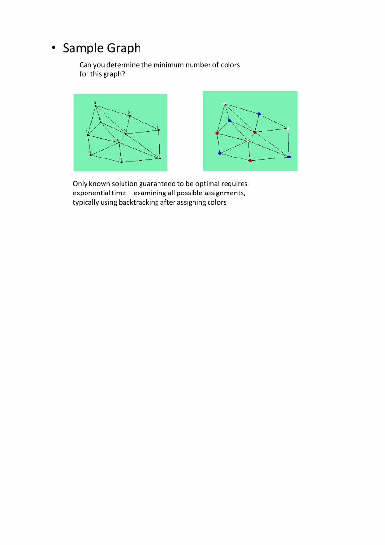
Sample Graph
Can you determine the minimum number of colorsfor this graph?
Only known solution guaranteed to be optimal requires
exponential time examining all possible assignments,
typically using backtracking after assigning colors
5/12/2018 Dynamic Prgming & Backtracking - slidepdf.com
http://slidepdf.com/reader/full/dynamic-prgming-backtracking 80/98
Graph Coloring
With these problems we can propose them asdecision problems or as optimization problems
The decision problem is slightly easier, but still is NPComplete
Decision Problem: Given G and a positive integer k,is there a coloring of G using at most k colors?
Optimization Problem: Given G, determine X(G), the
chromatic number, and produce an optimal coloringthat uses only X(G) colors.
D fi iti
5/12/2018 Dynamic Prgming & Backtracking - slidepdf.com
http://slidepdf.com/reader/full/dynamic-prgming-backtracking 81/98
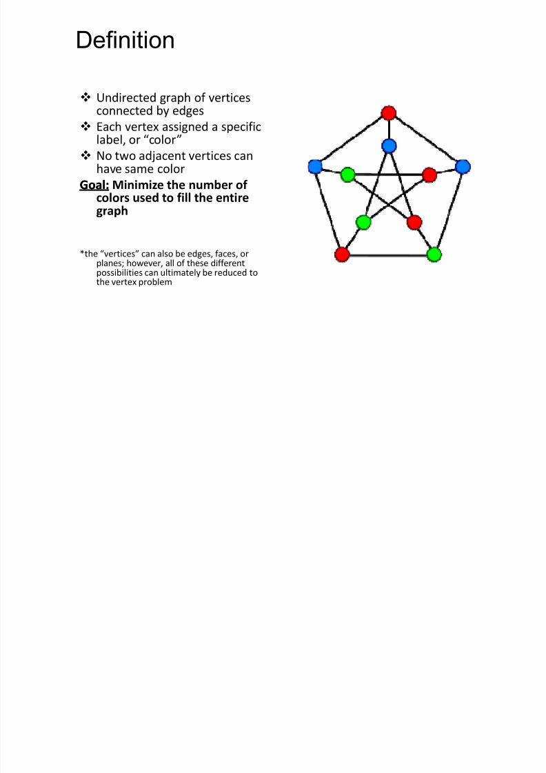
Def inition
Undirected graph of verticesconnected by edges
Each vertex assigned a specificlabel, or color
No two adjacent vertices can
have same colorGoal:Goal: Minimize the number of
colors used to fill the entire graph
*the vertices can also be edges, faces, orplanes; however, all of these differentpossibilities can ultimately be reduced tothe vertex problem
Obj ti
5/12/2018 Dynamic Prgming & Backtracking - slidepdf.com
http://slidepdf.com/reader/full/dynamic-prgming-backtracking 82/98
Objective
Perfor m extensive research on different heur istics for gr aph color ing
Analyze the results of each heur istic or algor ithm, and
compare the r unning times and eff iciency of each
Manipulate the data and gr aphs used in exper imentingwith each heur istic and obser ve the impact of such changes
Research current real-world applications and develop newpossible utilizations of the Gr aph Color ing Problem
Inspiration

5/12/2018 Dynamic Prgming & Backtracking - slidepdf.com
http://slidepdf.com/reader/full/dynamic-prgming-backtracking 83/98
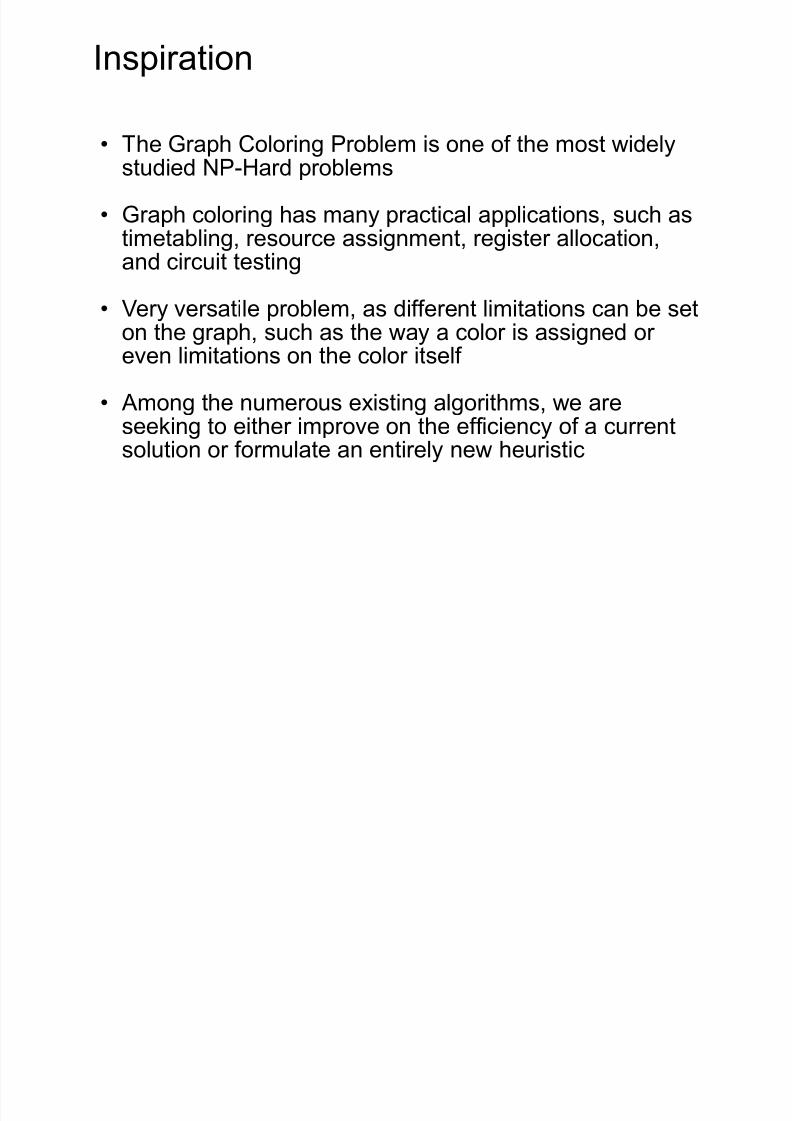
Inspir ation
The Gr aph Color ing Problem is one of the most widely studied NP-Har d problems
Gr aph color ing has many pr actical applications, such as
timetabling, resource assignment, register allocation,and circuit testing
Very versatile problem, as different limitations can be seton the gr aph, such as the way a color is assigned or
even limitations on the color itself
Among the numerous existing algor ithms, we are seeking to either improve on the eff iciency of a currentsolution or for mulate an entirely new heur istic
Algorithms
5/12/2018 Dynamic Prgming & Backtracking - slidepdf.com
http://slidepdf.com/reader/full/dynamic-prgming-backtracking 84/98
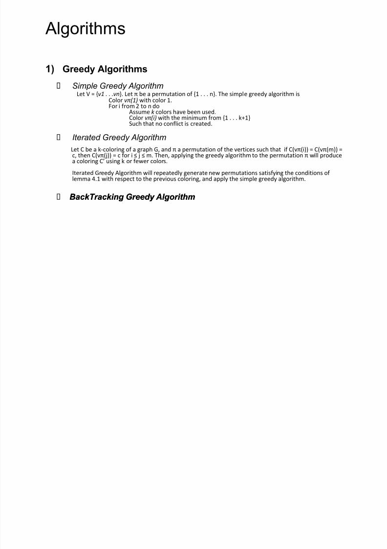
Algor ithms
1) Greedy Algorithms
Simple Greedy AlgorithmLet V = {v 1 . . .vn}. Let be a permutation of {1 . . . n}. The simple greedy algorithm is
Color v( 1 ) with color 1.For i from 2 to n do
Assume k colors have been used.
Color v( i) with the minimum from {1 . . . k+1}Such that no conflict is created.
I terated Greedy Algorithm
Let C be a k-coloring of a graph G, and a permutation of the vertices such that if C(v(i)) = C(v(m)) =c, then C(v(j)) = c for i j m. Then, applying the greedy algorithm to the permutation will producea coloring C using k or fewer colors.
Iterated Greedy Algorithm will repeatedly generate new permutations satisfying the conditions of
lemma 4.1 with respect to the previous coloring, and apply the simple greedy algorithm.
BackTracking BackTracking Greedy AlgorithmGreedy Algorithm
Algorithms
5/12/2018 Dynamic Prgming & Backtracking - slidepdf.com
http://slidepdf.com/reader/full/dynamic-prgming-backtracking 85/98
Algor ithms
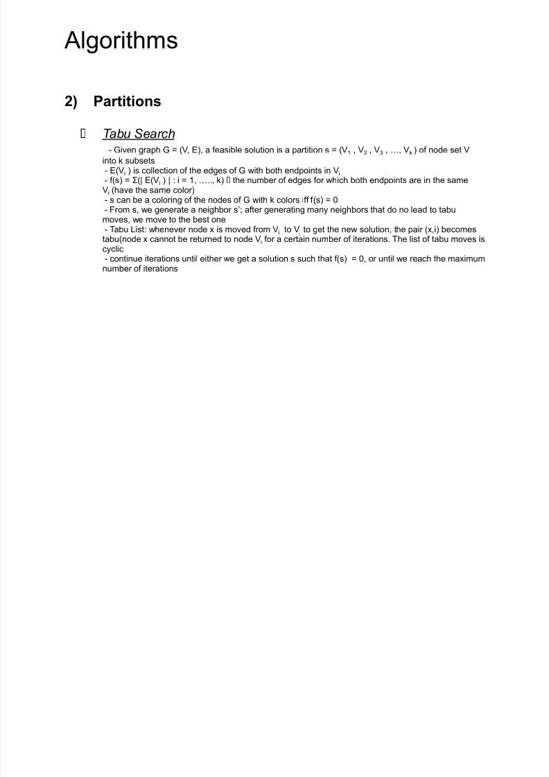
2) Partitions
T abu Search- Given gr aph G = (V, E), a feasible solution is a par tition s = (V1 , V2 , V3 , «, Vk ) of node set V
into k subsets
- E(Vi ) is collection of the edges of G with both endpoints in Vi
- f (s) = (| E(Vi ) | : i = 1, «.., k) the number of edges for which both endpoints are in the same Vi (have the same color )- s can be a color ing of the nodes of G with k colors iff f (s) = 0- From s, we gener ate a neighbor s¶; af ter gener ating many neighbors that do no lead to tabumoves, we move to the best one- Tabu List: whenever node x is moved from Vi to V j to get the new solution, the pair (x,i) becomes tabu(node x cannot be retur ned to node Vi for a cer tain number of iter ations. The list of tabu moves is
cyclic- continue iter ations until either we get a solution s such that f (s) = 0, or until we reach the maximumnumber of iter ations
Algorithms
5/12/2018 Dynamic Prgming & Backtracking - slidepdf.com
http://slidepdf.com/reader/full/dynamic-prgming-backtracking 86/98
Algor ithms
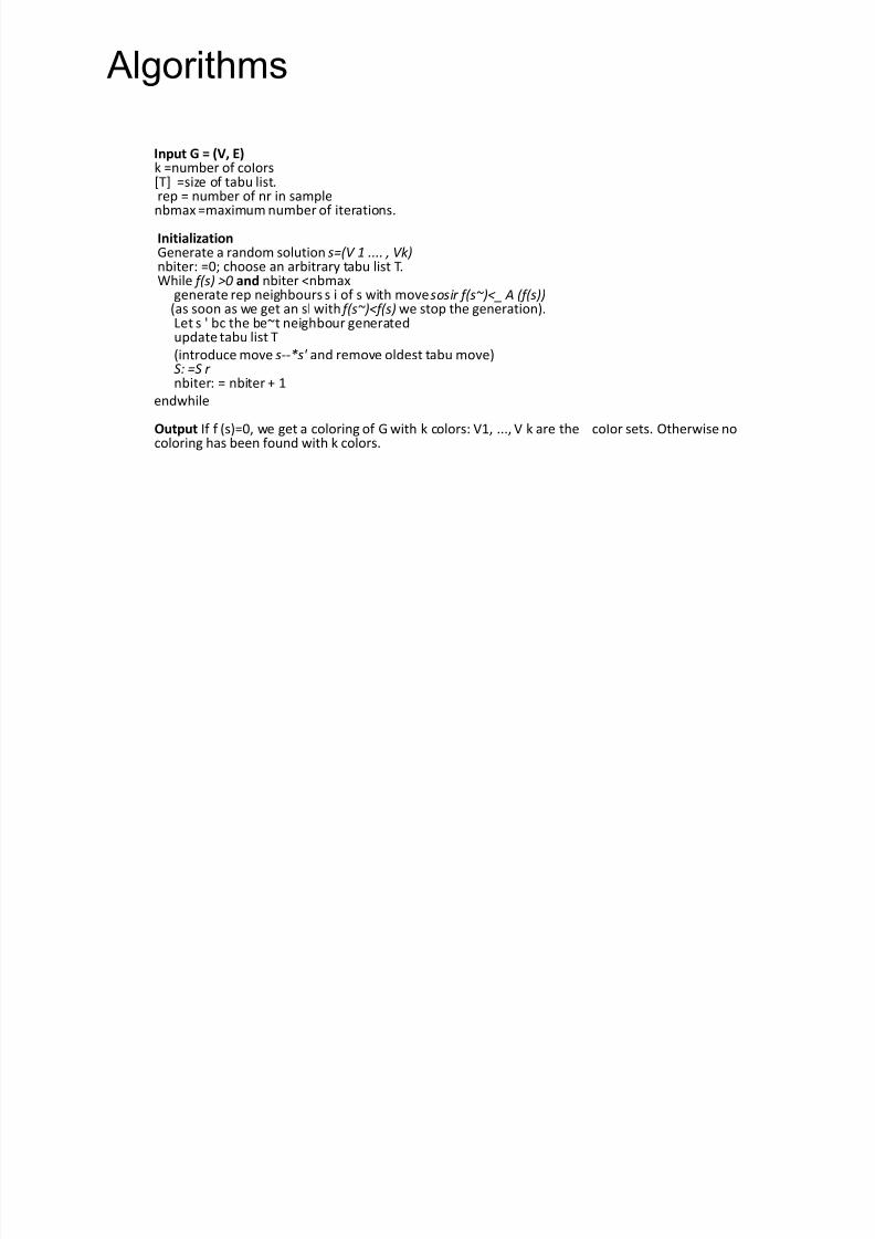
Input G = (V, E)k =number of coIors[T] =size of tabu list.rep = number of nr in samplenbmax =maximum number of iterations.
InitializationGenerate a random solution s=( V 1 .... , V k )
nbiter: =0; choose an arbitrary tabu list T.While f ( s) >0 and nbiter <nbmaxgenerate rep neighbours s i of s with move sosir f ( s~)<_ A ( f ( s))
(as soon as we get an sl with f ( s~)<f ( s) we stop the generation).Let s ' bc the be~t neighbour generatedupdate tabu list T
(introduce move s--*s' and remove oldest tabu move)S: =S r nbiter: = nbiter + 1
endwhile
Output If f (s)=0, we get a coloring of G with k colors: V1, ..., V k are the coIor sets. Otherwise nocoloring has been found with k colors.
Algorithms
5/12/2018 Dynamic Prgming & Backtracking - slidepdf.com
http://slidepdf.com/reader/full/dynamic-prgming-backtracking 87/98
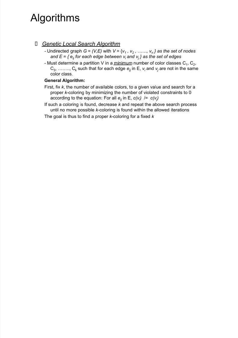
Algor ithms
Genetic Local Search Algorithm
- Undirected gr aph G = (V,E) with V = {v 1 , v 2 , ««, v n } as the set of nodes
and E = { eij for each edge between v i and v j } as the set of edges
- Must deter mine a par tition V in a minimum number of color classes C1, C2,
C3, ««.., Ck such that for each edge eij in E, v i and v j are not in the same
color class.General Algorithm:
First, f ix k , the number of available colors, to a given value and search for a
proper k -color ing by minimizing the number of violated constr aints to 0
accor ding to the equation: For all eij in E, c(v i ) /= c(v j )
If such a color ing is found, decrease k and repeat the above search process
until no more possible k -color ing is found within the allowed iter ationsThe goal is thus to f ind a proper k -color ing for a f ixed k
Al ith
5/12/2018 Dynamic Prgming & Backtracking - slidepdf.com
http://slidepdf.com/reader/full/dynamic-prgming-backtracking 88/98
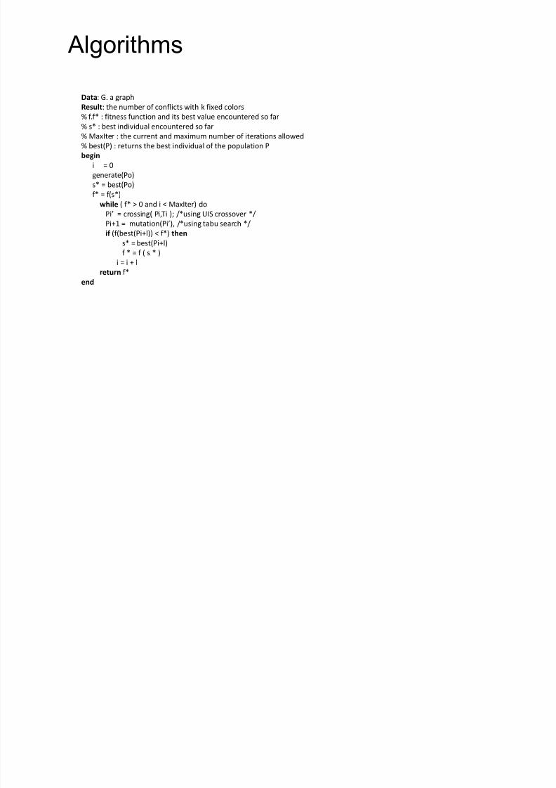
Algor ithms
Data: G. a graph
Result: the number of conflicts with k fixed colors
% f.f * : fitness function and its best value encountered so far
% s* : best individual encountered so far
% MaxIter : the current and maximum number of iterations allowed
% best(P) : returns the best individual of the population P
begin
i = 0
generate(Po)s* = best(Po)
f * = f(s*)
while ( f * > 0 and i < MaxIter) do
Pi = crossing( Pi,Ti ); /*using UIS crossover */
Pi+1 = mutation(Pi), /*using tabu search */
if (f(best(Pi+l)) < f *) then
s* = best(Pi+l)
f *
= f ( s*
)i = i + l
return f *
end
Experiment
5/12/2018 Dynamic Prgming & Backtracking - slidepdf.com
http://slidepdf.com/reader/full/dynamic-prgming-backtracking 89/98
Exper iment
Run algor ithms on different gr aphs, recor d number of colors used, and f ind the optimal heur istic
Modify number of edges and number of cliques in a gr aph
and analyze the effects of edge and clique density
5/12/2018 Dynamic Prgming & Backtracking - slidepdf.com
http://slidepdf.com/reader/full/dynamic-prgming-backtracking 90/98
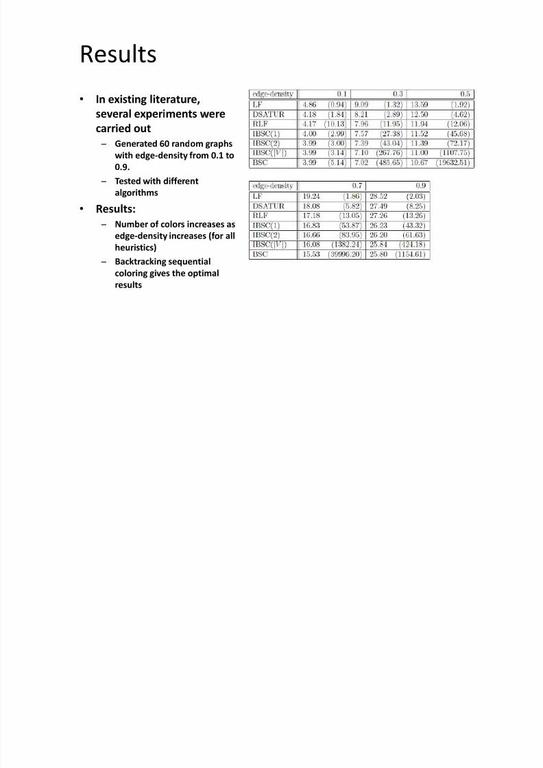
Results
In existing literature,
several experiments were
carried out
± Generated 60 random graphs
with edge-density f rom 0.1 to
0.9. ± Tested with different
algorithms
Results:
± Number of colors increases as
edge-density increases (f or all
heuristics) ± Backtracking sequential
coloring gives the optimal
results
5/12/2018 Dynamic Prgming & Backtracking - slidepdf.com
http://slidepdf.com/reader/full/dynamic-prgming-backtracking 91/98
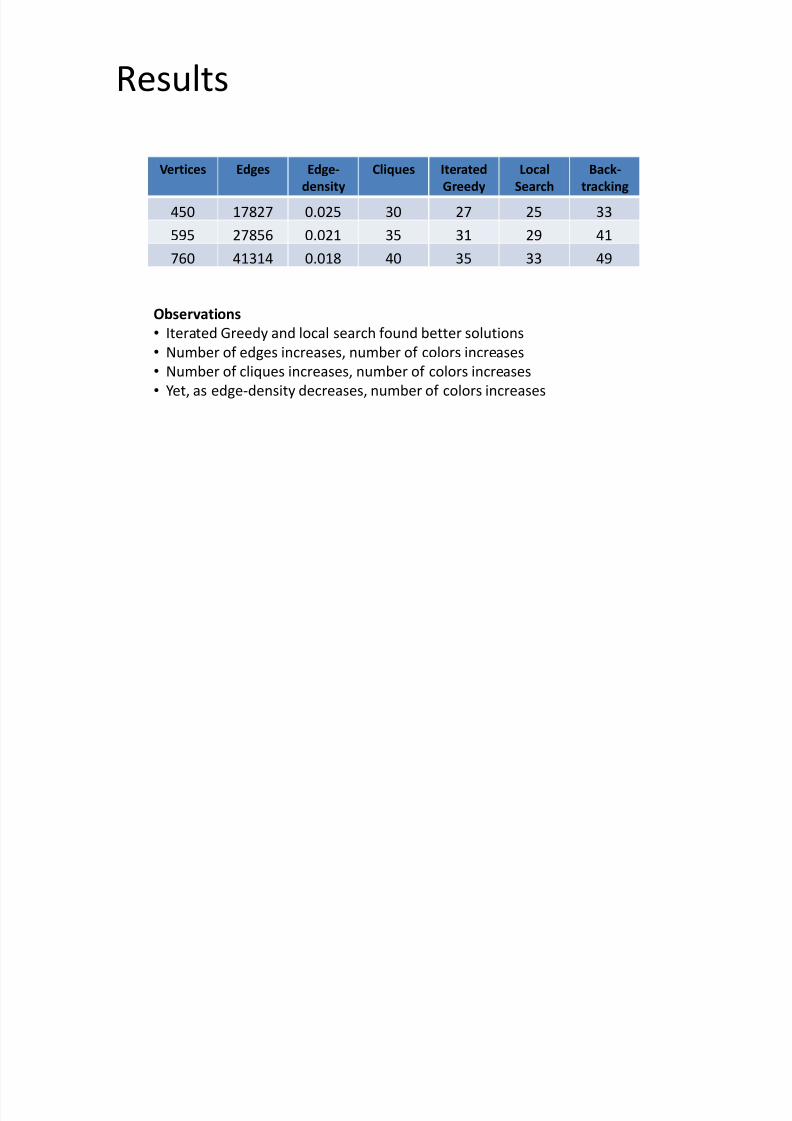
Results
Vertices Edges Edge-
density
Cliques Iterated
Greedy
Local
Search
Back-
tracking
450 17827 0.025 30 27 25 33
595 27856 0.021 35 31 29 41
760 41314 0.018 40 35 33 49
Observations
Iterated Greedy and local search found better solutions
Number of edges increases, number of colors increases
Number of cliques increases, number of colors increases
Yet, as edge-density decreases, number of colors increases
5/12/2018 Dynamic Prgming & Backtracking - slidepdf.com
http://slidepdf.com/reader/full/dynamic-prgming-backtracking 92/98
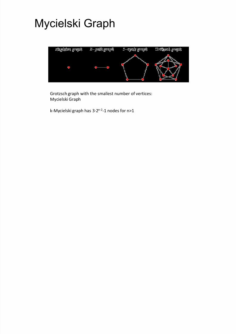
Mycielski Gr aph
Grotzsch graph with the smallest number of vertices:
Mycielski Graph
k-Mycielski graph has 3·2n-2-1 nodes for n>1
M i l ki G h

5/12/2018 Dynamic Prgming & Backtracking - slidepdf.com
http://slidepdf.com/reader/full/dynamic-prgming-backtracking 93/98
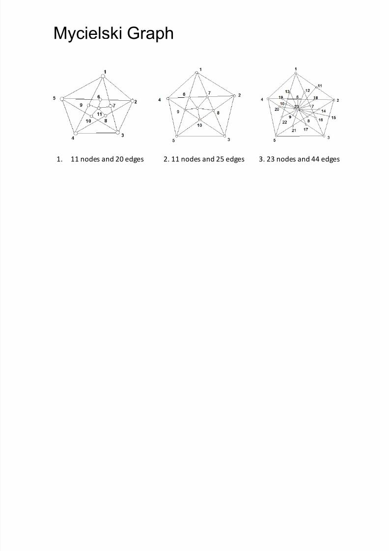
Mycielski Gr aph
1. 11 nodes and 20 edges 2. 11 nodes and 25 edges 3. 23 nodes and 44 edges
Results

5/12/2018 Dynamic Prgming & Backtracking - slidepdf.com
http://slidepdf.com/reader/full/dynamic-prgming-backtracking 94/98
Results
AlgorithmsNumber
of colors
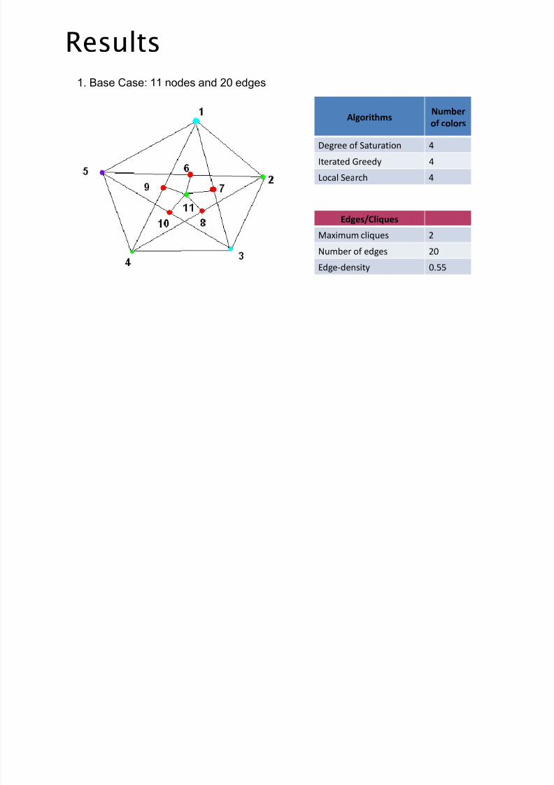
Degree of Saturation 4
Iterated Greedy 4
Local Search 4
Edges/Cliques
Maximum cliques 2
Number of edges 20Edge-density 0.55
1. Base Case: 11 nodes and 20 edges
Results

5/12/2018 Dynamic Prgming & Backtracking - slidepdf.com
http://slidepdf.com/reader/full/dynamic-prgming-backtracking 95/98
Results
AlgorithmsNumber
of colors
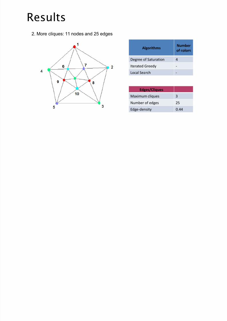
Degree of Saturation 4
Iterated Greedy -
Local Search -
Edges/Cliques
Maximum cliques 3
Number of edges 25Edge-density 0.44
2. More cliques: 11 nodes and 25 edges
Results

5/12/2018 Dynamic Prgming & Backtracking - slidepdf.com
http://slidepdf.com/reader/full/dynamic-prgming-backtracking 96/98
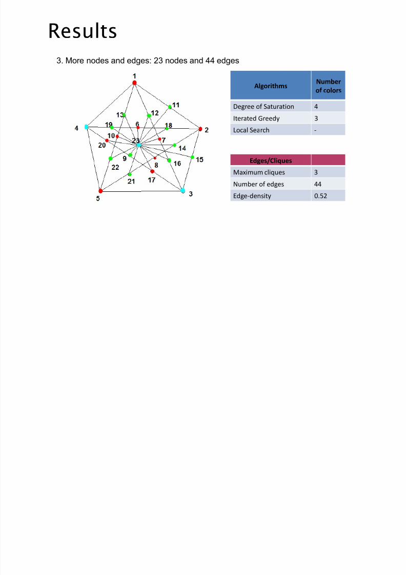
Results
AlgorithmsNumber
of colors
Degree of Saturation 4
Iterated Greedy 3
Local Search -
Edges/Cliques
Maximum cliques 3
Number of edges 44Edge-density 0.52
3. More nodes and edges: 23 nodes and 44 edges

5/12/2018 Dynamic Prgming & Backtracking - slidepdf.com
http://slidepdf.com/reader/full/dynamic-prgming-backtracking 97/98
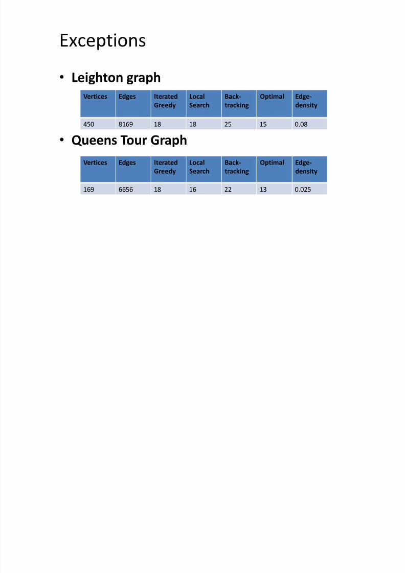
Exceptions
Leighton graph
Queens Tour Graph
Vertices Edges Iterated
Greedy
Local
Search
Back-
tracking
Optimal Edge-
density
450 8169 18 18 25 15 0.08
Vertices Edges Iterated
Greedy
Local
Search
Back-
tracking
Optimal Edge-
density
169 6656 18 16 22 13 0.025

5/12/2018 Dynamic Prgming & Backtracking - slidepdf.com
http://slidepdf.com/reader/full/dynamic-prgming-backtracking 98/98
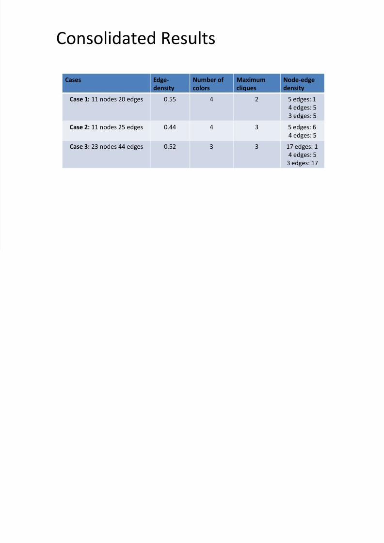
Consolidated Results
Cases Edge-
density
Number of
colors
Maximum
cliques
Node-edge
density
Case 1: 11 nodes 20 edges 0.55 4 2 5 edges: 1
4 edges: 5
3 edges: 5
Case 2: 11 nodes 25 edges 0.44 4 3 5 edges: 6
4 edges: 5
Case 3: 23 nodes 44 edges 0.52 3 3 17 edges: 1
4 edges: 5
3 edges: 17