DSLP Calculations by Razevig Method
17
ψ DANIELIAUTOMATION ELECTRICAL GENERAL SYSTEMS – GROUNDING CALCULATIONS 1 Table of contents - Table of contents - .............................................................................................................................1 1 AIM OF THE STUDY..........................................................................................................................2 2 DEFINITIONS AND THERMINOLOGY..............................................................................................2 3 SOFTWARE USED AND INPUT DATA.............................................................................................2 3.1 ELECTRICAL DATA.........................................................................................................................2 3.2 PHYSICAL DATA.............................................................................................................................3 3.3 GEOMETRICAL DATA.....................................................................................................................3 3.4 REFERENCE STANDARD...............................................................................................................4 4 DESIGN AND VERIFICATION CALCULATIONS..............................................................................5 4.1 DESIGN OF THE GRID CONDUCTORS.........................................................................................5 4.2 VERIFICATION OF THE EARTHING GRID LAYOUT.....................................................................6 5 CONCLUSIONS................................................................................................................................17 6 ANNEXES.........................................................................................................................................17
-
Upload
rajeshchauhan -
Category
Documents
-
view
1.390 -
download
67
description
Direct Stroke Lightning Protections. Calculatiion. Direct Stroke Lightning Protections. Calculatiion. Downloaded from Scribd. DSLP Calculations by Razevig MethodDirect Stroke Lightning Protections. Calculatiion. Direct Stroke Lightning Protections. Calculatiion. Downloaded from Scribd. DSLP Calculations by Razevig Method
Transcript of DSLP Calculations by Razevig Method
ψDANIELIAUTOMATION ELECTRICAL GENERAL SYSTEMS – GROUNDING CALCULATIONS 1
Table of contents -
Table of contents - .............................................................................................................................1
1 AIM OF THE STUDY..........................................................................................................................2
2 DEFINITIONS AND THERMINOLOGY..............................................................................................2
3 SOFTWARE USED AND INPUT DATA.............................................................................................2
3.1 ELECTRICAL DATA.........................................................................................................................2
3.2 PHYSICAL DATA.............................................................................................................................3
3.3 GEOMETRICAL DATA.....................................................................................................................3
3.4 REFERENCE STANDARD...............................................................................................................4
4 DESIGN AND VERIFICATION CALCULATIONS..............................................................................5
4.1 DESIGN OF THE GRID CONDUCTORS.........................................................................................5
4.2 VERIFICATION OF THE EARTHING GRID LAYOUT.....................................................................6
5 CONCLUSIONS................................................................................................................................17
6 ANNEXES.........................................................................................................................................17

ψDANIELIAUTOMATION ELECTRICAL GENERAL SYSTEMS – GROUNDING CALCULATIONS 2
1 AIM OF THE STUDY
This report focuses on the calculations made to design the primary earthing network of the UNICOIL Galvanization Plant.The place is located in Jubail Industrial City (Al Jubail , Kingdom of Saudi Arabia), at about 10 km from the Arabian Gulf.The overall area on the plant has a nearly rectangular shape covering a 750x250 m surface.A primary earthing network is already realised on the Painting Line area so that the Galvanization area will be served by an extension of this existing network. The calculations carried out for the design of the earthing network will then account for the overall grid, considering that the former and the new one will be interconnected.
2 DEFINITIONS AND THERMINOLOGY
According to European Harmonisation Documents CENELEC HD 637 S1 will be used following symbols (brackets the corresponding definitions IEEE Std 80-2000):
- Rb (Rb) = resistance of the human body- Re (Rg) = earthing resistance- Ue (GPR) = ground potential rise- Ues = earth surface potential - Ut (Et) = touch voltage- Ust = touch voltage, as measured without presence of human body- Utp (Rb*Ib) = permissible touch voltage- Us (Es) = step voltage- Uss = step voltage, as measured without presence of human body- Usp (Rb*Ib) = permissible step voltage- If (If) = fault current- Id (Ie) = drawn current- Ie (Ig) = earthing current- ts (ts) = intervention time of protections
The following terminology will be preferred in this report:- “earth” instead of “ground”- “earthing grid” to refer to the primary earthing network- “down lead conductors” to refer to the conductors which connect the metallic masses to the primary earthing network.Other terms will be in accordance with the used standards.
3 SOFTWARE USED AND INPUT DATA
The software used is GSA (Grounding System and Soil Structure Analysis), a tool whose flow chart is explained in Annex01 and which has been validated for several situations.Inputs for the program are:
- electrical data: single phase to earth short circuit currents (If), currents drawn by earthwire(s) and cable shields (Id), intervention time of protections (ts)- physical data: soil characteristics- geometrical data: geometry of the earthing network under study- reference standard limits: maximum touch and step voltages (Utp, Usp)
3.1 ELECTRICAL DATA
The steel plant is fed from a 110/34.5 kV substation via a MV XLPE cables 95 mm2 line at 34,5 kV. The three-phase short circuit power at the substation (at about 2 km from the plant) is 1500 MVA, earth fault current and fault duration are not available from UNICOIL.With reference to the above and to similar conditions of supply networks, the single phase to earth fault current at the MV coupling point has been conservatively supposed to be:
- If = 15.000 A
A portion of the fault current is drawn by the feeding cables shield.
ψDANIELIAUTOMATION ELECTRICAL GENERAL SYSTEMS – GROUNDING CALCULATIONS 3
According to typical data (see European Harmonisation Documents CENELEC HD 637 S1), this portion amounts to:
- Id/If = 0,55
The current that the earthing grid is called to draw is then:
- Ie = If – Id = 6.750 A
The intervention time of protections (fault duration) has been supposed to be:
- ts = 1,00 s
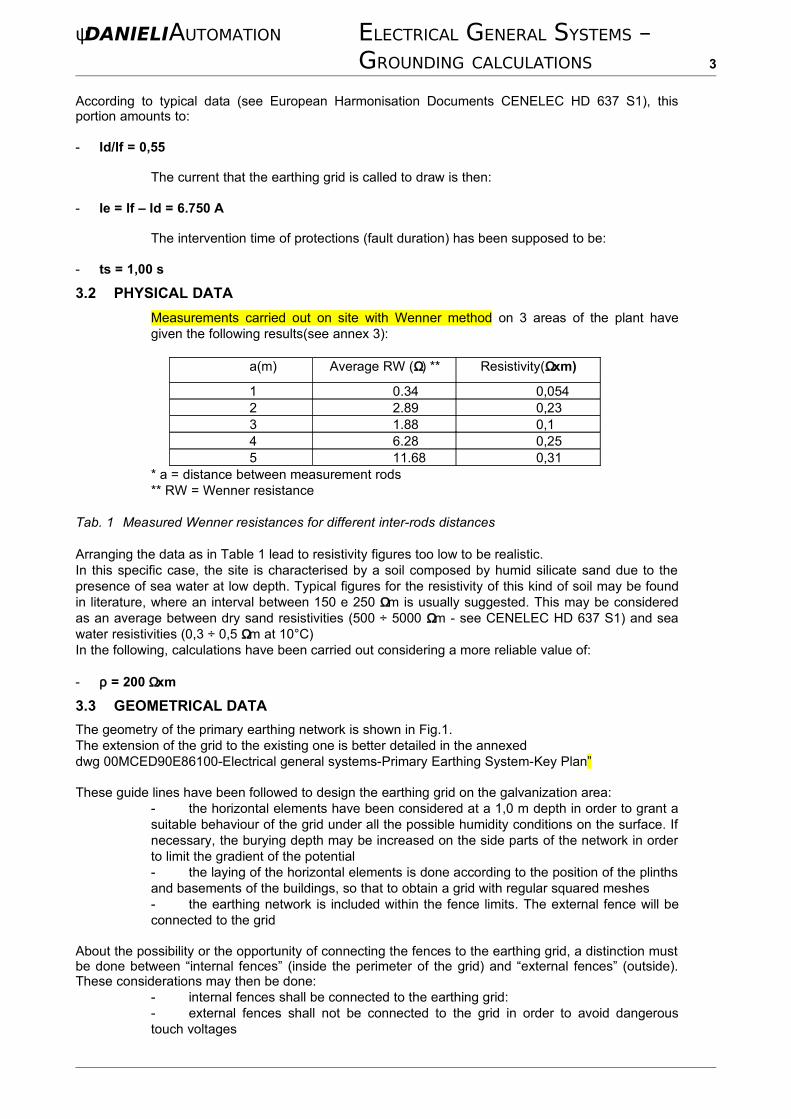
3.2 PHYSICAL DATA
Measurements carried out on site with Wenner method on 3 areas of the plant have given the following results(see annex 3):
a(m) Average RW (Ω) ** Resistivity(Ωxm)
1 0.34 0,0542 2.89 0,233 1.88 0,14 6.28 0,255 11.68 0,31
* a = distance between measurement rods** RW = Wenner resistance
Tab. 1 Measured Wenner resistances for different inter-rods distances
Arranging the data as in Table 1 lead to resistivity figures too low to be realistic.In this specific case, the site is characterised by a soil composed by humid silicate sand due to the presence of sea water at low depth. Typical figures for the resistivity of this kind of soil may be found in literature, where an interval between 150 e 250 Ωm is usually suggested. This may be considered as an average between dry sand resistivities (500 ÷ 5000 Ωm - see CENELEC HD 637 S1) and sea water resistivities (0,3 ÷ 0,5 Ωm at 10°C)In the following, calculations have been carried out considering a more reliable value of:
- ρ = 200 Ωxm
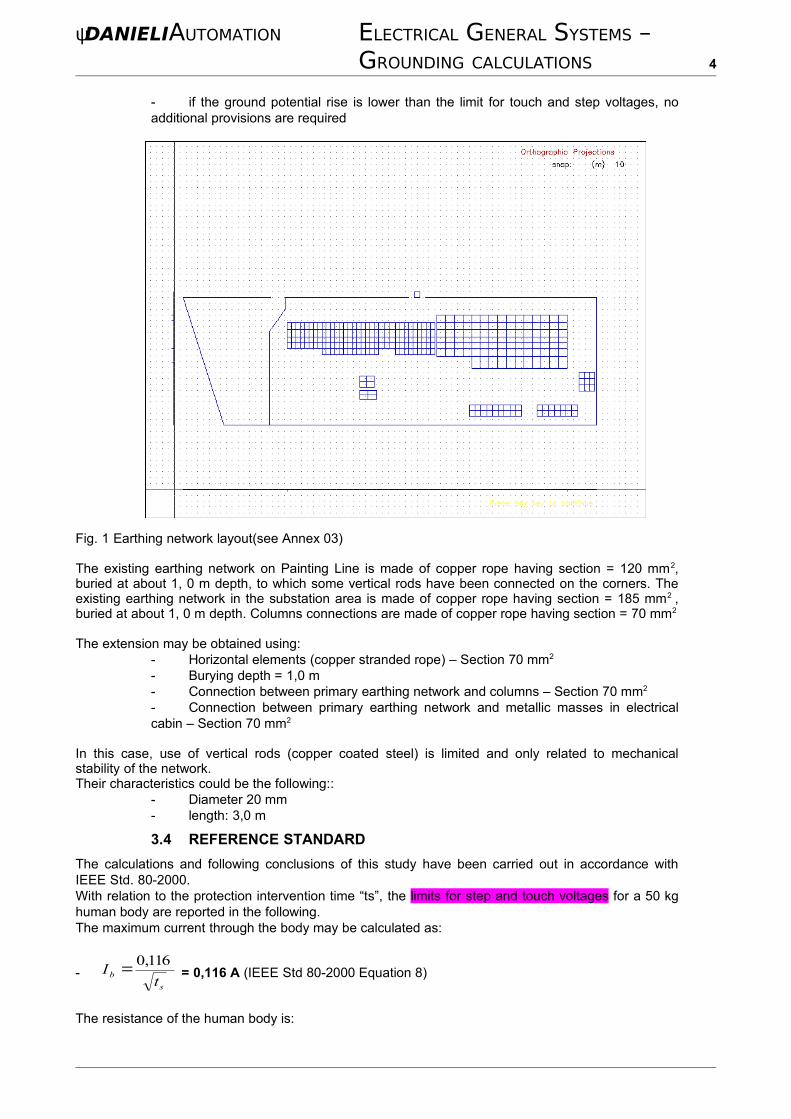
3.3 GEOMETRICAL DATA
The geometry of the primary earthing network is shown in Fig.1. The extension of the grid to the existing one is better detailed in the annexed dwg 00MCED90E86100-Electrical general systems-Primary Earthing System-Key Plan”
These guide lines have been followed to design the earthing grid on the galvanization area:- the horizontal elements have been considered at a 1,0 m depth in order to grant a suitable behaviour of the grid under all the possible humidity conditions on the surface. If necessary, the burying depth may be increased on the side parts of the network in order to limit the gradient of the potential- the laying of the horizontal elements is done according to the position of the plinths and basements of the buildings, so that to obtain a grid with regular squared meshes- the earthing network is included within the fence limits. The external fence will be connected to the grid
About the possibility or the opportunity of connecting the fences to the earthing grid, a distinction must be done between “internal fences” (inside the perimeter of the grid) and “external fences” (outside). These considerations may then be done:
- internal fences shall be connected to the earthing grid:- external fences shall not be connected to the grid in order to avoid dangerous touch voltages
ψDANIELIAUTOMATION ELECTRICAL GENERAL SYSTEMS – GROUNDING CALCULATIONS 4
- if the ground potential rise is lower than the limit for touch and step voltages, no additional provisions are required
Fig. 1 Earthing network layout(see Annex 03)
The existing earthing network on Painting Line is made of copper rope having section = 120 mm2, buried at about 1, 0 m depth, to which some vertical rods have been connected on the corners. The existing earthing network in the substation area is made of copper rope having section = 185 mm2 , buried at about 1, 0 m depth. Columns connections are made of copper rope having section = 70 mm2
The extension may be obtained using:- Horizontal elements (copper stranded rope) – Section 70 mm2
- Burying depth = 1,0 m- Connection between primary earthing network and columns – Section 70 mm2
- Connection between primary earthing network and metallic masses in electrical cabin – Section 70 mm2
In this case, use of vertical rods (copper coated steel) is limited and only related to mechanical stability of the network.Their characteristics could be the following::
- Diameter 20 mm- length: 3,0 m
3.4 REFERENCE STANDARD
The calculations and following conclusions of this study have been carried out in accordance with IEEE Std. 80-2000.With relation to the protection intervention time “ts”, the limits for step and touch voltages for a 50 kg human body are reported in the following.The maximum current through the body may be calculated as:
-s
bt
I116,0= = 0,116 A (IEEE Std 80-2000 Equation 8)
The resistance of the human body is:

ψDANIELIAUTOMATION ELECTRICAL GENERAL SYSTEMS – GROUNDING CALCULATIONS 5
- Rb = 1000 Ω (IEEE Std 80-2000 Equation 10)
With reference to a surface resistivity of the soil equal to 200 Ωm (see 1.2), the maximum touch and step voltages which may be measured by an instrument having an infinite internal impedance, are:
- E touch = Ib * (Rb + 1,5*ρ) = 150,8 V (IEEE Std 80-2000 Equation 17)
- E step = Ib * (Rb + 6,0*ρ) = 255,2 V (IEEE Std 80-2000 Equation 18)
The maximum voltage on the human body in both case is instead:
- Eb = Rb * Ib = 116,0 V
Then:
- Utp = 116,0 V- Usp = 116,0 V
4 DESIGN AND VERIFICATION CALCULATIONS
The calculations for design and check of the primary earthing network have been carried out with calculation code GSA (see Annex01 for details).
4.1 DESIGN OF THE GRID CONDUCTORS
The verification of the section of the grid conductor for thermal purposes may be obtained comparing the maximum current density during fault condition by formula:
-a
m
rrc TK
TK
t
TCAP
A
I
++
⋅=−
0
04
ln10
ρα (IEEE Std 80-2000 Equation 37)
where:- I/A: maximum current density (kA/mm2)
- Tm: is the maximum allowable temperature (°C)- Ta: is the ambient ore initial temperature (°C)- Tr: is the reference temperature for material constant (°C)- αo: is the thermal coefficient of resistivity at 0°C (1/°C)- αr: is the thermal coefficient of resistivity at reference temperature Tr (1/°C)- ρr: is the resistivity of the ground conductor at the reference temperature (µΩ cm)- Ko = 1/αo- tc: is the duration of fault current (s)- TCAP: is the thermal capacity (J/°C cm3)
The following values have been considered for the above variables (IEEE Std 80-2000 Table 1) :- Tm: 300°C- Ta: 35 °C- Tr: 20 °C- αo: 1/242 1/°C- αr: 0,00381 1/°C- ρr: 1,78 µΩ cm- Ko = 242 °C- tc: 1 s- TCAP: 3,42 J/°C cm3
which yield:- I/A = 0,184 kA/mm2
A copper conductor having section S = 70 mm2 has then a maximum admissible current = 12,880 A. This section is suitable to withstand the whole earth current, although it may be considered that a
ψDANIELIAUTOMATION ELECTRICAL GENERAL SYSTEMS – GROUNDING CALCULATIONS 6
earth current will always follow at least two different paths of comparable impedance. With reference to the above it is possible to assume that the max fault current that the earthing copper conductor can bear is 12.8x2=25.6 kA. This assures a correct thermal design for the earthing conductor.
The calculation of the down leads to grid conductor may be calculated with the same procedure.
Considering the following values:- Tm: 200°C- Ta: 50 °C- Tr: 20 °C- αo: 1/242 1/°C- αr: 0,00381 1/°C- ρr: 1,78 µΩ cm- Ko = 242 °C- tc: 1 s- TCAP: 3,42 J/°C cm3
the current density G my be calculated as:- I/A = 0,145 kA/mm2
A copper conductor having section S = 70 mm2 has then a maximum admissible current = 10,120 A, being suitable to withstand the overall earth current. This assures a correct thermal design for the down lead conductor.
The sections for the grid and down lead conductors are correctly chosen also with reference to the short circuit current which is carried by the earthing grid.
If an intervention time of the protections is assumed to be 0.1 s, the maximum admissible currents for the earthing grid and down lead conductors are respectively 70*579 = 40.5 k A and 70*455 = 31.85 kA. For each electrical cabin, two lead conductors will be instead installed: assuming that a current injected in the grid will always be divided in at least two branches, the limit short circuit current for thermal design is about 60 kA.
4.2 VERIFICATION OF THE EARTHING GRID LAYOUT
The verification of the layout as chosen with criteria illustrated in 1.3 may be obtained with the following steps:
- calculation of earth resistance and ground potential rise: if the ground potential rise is lower than the maximum step and touch voltages, the earthing grid is to be considered correctly designed. Conversely, the following must be considered;- calculation of step and touch voltages and comparison with the limits as given by the standard IEEE 80: if these values are lower than the limits, the earthing grid is to be considered correctly designed.
The calculated resistance of the grid calculated by GSA is:
- Re = 0,254 Ω
The ground potential rise will then be:
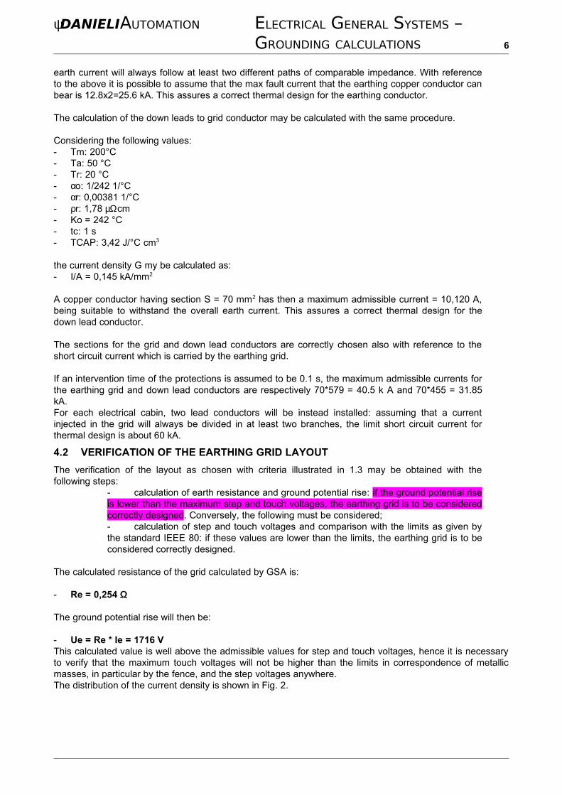
- Ue = Re * Ie = 1716 VThis calculated value is well above the admissible values for step and touch voltages, hence it is necessary to verify that the maximum touch voltages will not be higher than the limits in correspondence of metallic masses, in particular by the fence, and the step voltages anywhere.The distribution of the current density is shown in Fig. 2.
ψDANIELIAUTOMATION ELECTRICAL GENERAL SYSTEMS – GROUNDING CALCULATIONS 7
Fig. 2 Distribution of linear current density on the earthing network(see Annex 03)
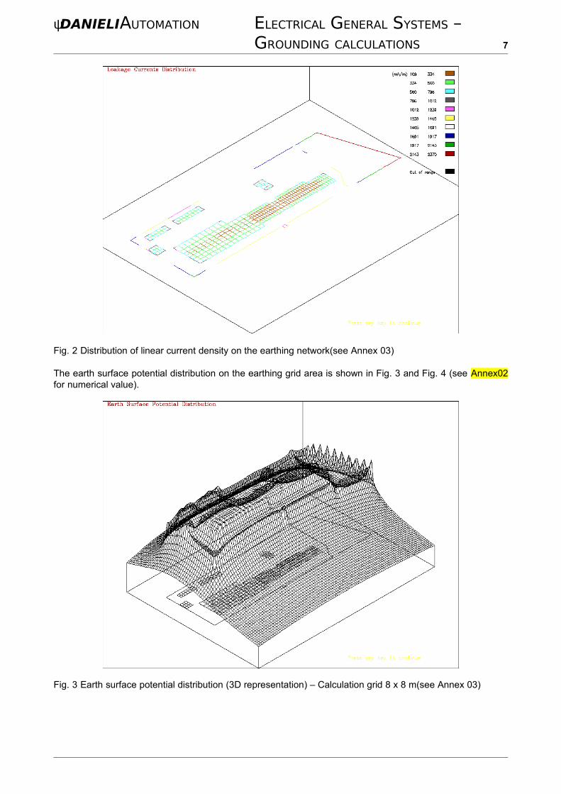
The earth surface potential distribution on the earthing grid area is shown in Fig. 3 and Fig. 4 (see Annex02 for numerical value).
Fig. 3 Earth surface potential distribution (3D representation) – Calculation grid 8 x 8 m(see Annex 03)
ψDANIELIAUTOMATION ELECTRICAL GENERAL SYSTEMS – GROUNDING CALCULATIONS 8
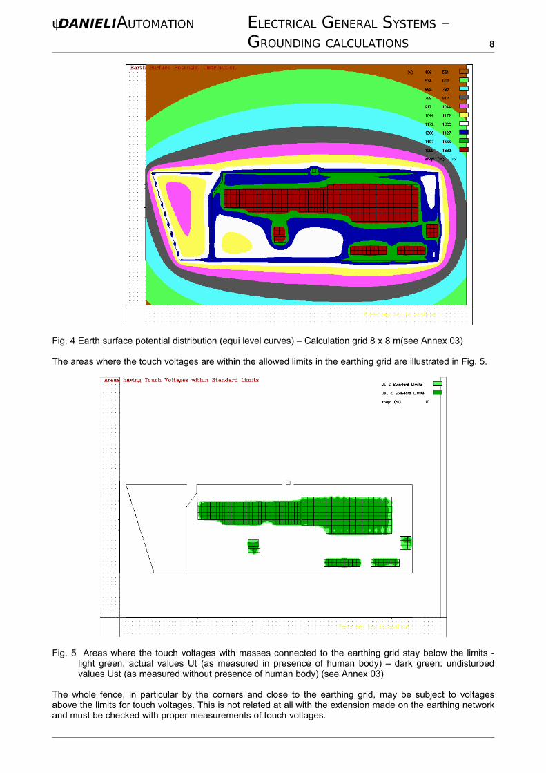
Fig. 4 Earth surface potential distribution (equi level curves) – Calculation grid 8 x 8 m(see Annex 03)
The areas where the touch voltages are within the allowed limits in the earthing grid are illustrated in Fig. 5.
Fig. 5 Areas where the touch voltages with masses connected to the earthing grid stay below the limits - light green: actual values Ut (as measured in presence of human body) – dark green: undisturbed values Ust (as measured without presence of human body) (see Annex 03)
The whole fence, in particular by the corners and close to the earthing grid, may be subject to voltages above the limits for touch voltages. This is not related at all with the extension made on the earthing network and must be checked with proper measurements of touch voltages.
ψDANIELIAUTOMATION ELECTRICAL GENERAL SYSTEMS – GROUNDING CALCULATIONS 9
If these measurements will confirm this, it will be advisable to cover these areas with an insulating layer (around 1.5 m beyond the fence and 1.5 m inside the fence) must be considered (bitumen or crushed rock) to limit the touch voltages. The same for some areas of plant, in particular near the corner.
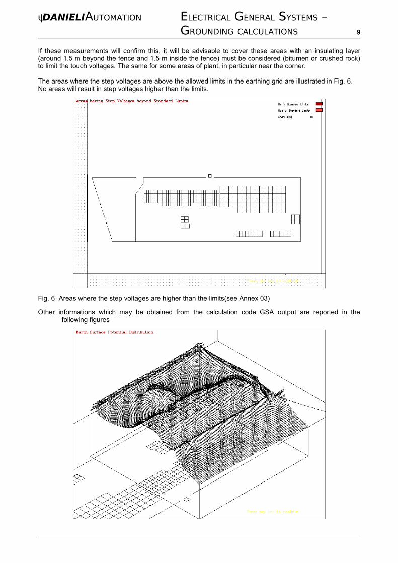
The areas where the step voltages are above the allowed limits in the earthing grid are illustrated in Fig. 6. No areas will result in step voltages higher than the limits.
Fig. 6 Areas where the step voltages are higher than the limits(see Annex 03)
Other informations which may be obtained from the calculation code GSA output are reported in the following figures
ψDANIELIAUTOMATION ELECTRICAL GENERAL SYSTEMS – GROUNDING CALCULATIONS 10
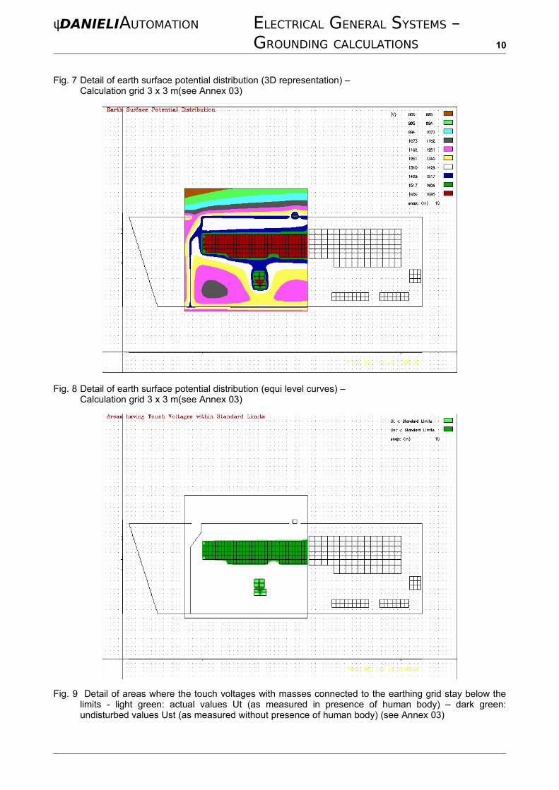
Fig. 7 Detail of earth surface potential distribution (3D representation) – Calculation grid 3 x 3 m(see Annex 03)
Fig. 8 Detail of earth surface potential distribution (equi level curves) – Calculation grid 3 x 3 m(see Annex 03)
Fig. 9 Detail of areas where the touch voltages with masses connected to the earthing grid stay below the limits - light green: actual values Ut (as measured in presence of human body) – dark green: undisturbed values Ust (as measured without presence of human body) (see Annex 03)
ψDANIELIAUTOMATION ELECTRICAL GENERAL SYSTEMS – GROUNDING CALCULATIONS 11
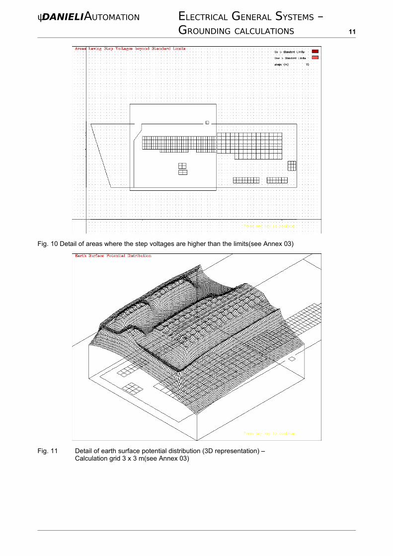
Fig. 10 Detail of areas where the step voltages are higher than the limits(see Annex 03)
Fig. 11 Detail of earth surface potential distribution (3D representation) – Calculation grid 3 x 3 m(see Annex 03)
ψDANIELIAUTOMATION ELECTRICAL GENERAL SYSTEMS – GROUNDING CALCULATIONS 12
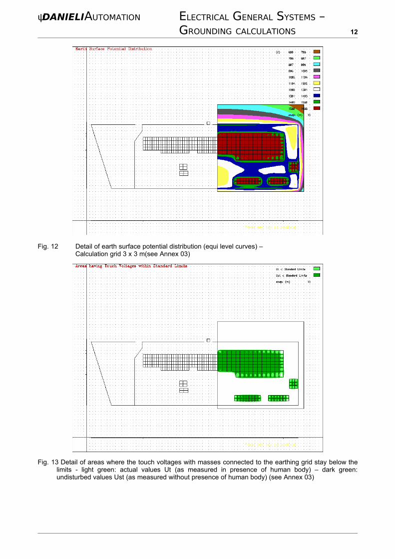
Fig. 12 Detail of earth surface potential distribution (equi level curves) – Calculation grid 3 x 3 m(see Annex 03)
Fig. 13 Detail of areas where the touch voltages with masses connected to the earthing grid stay below the limits - light green: actual values Ut (as measured in presence of human body) – dark green: undisturbed values Ust (as measured without presence of human body) (see Annex 03)
ψDANIELIAUTOMATION ELECTRICAL GENERAL SYSTEMS – GROUNDING CALCULATIONS 13
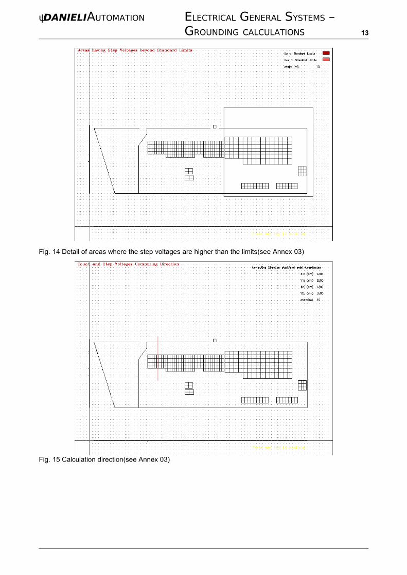
Fig. 14 Detail of areas where the step voltages are higher than the limits(see Annex 03)
Fig. 15 Calculation direction(see Annex 03)
ψDANIELIAUTOMATION ELECTRICAL GENERAL SYSTEMS – GROUNDING CALCULATIONS 14
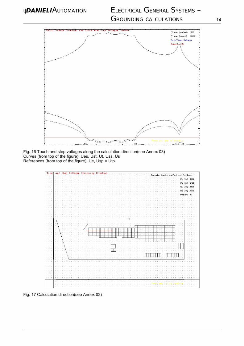
Fig. 16 Touch and step voltages along the calculation direction(see Annex 03)Curves (from top of the figure): Ues, Ust, Ut, Uss, UsReferences (from top of the figure): Ue, Usp = Utp
Fig. 17 Calculation direction(see Annex 03)
ψDANIELIAUTOMATION ELECTRICAL GENERAL SYSTEMS – GROUNDING CALCULATIONS 15
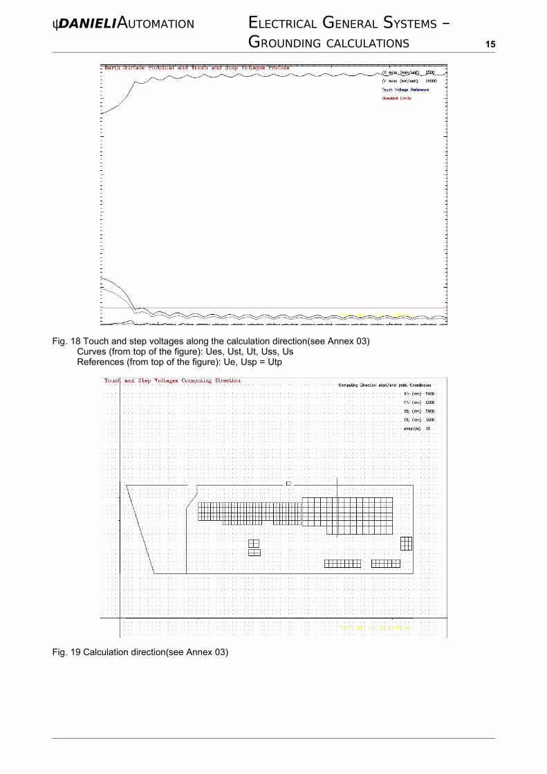
Fig. 18 Touch and step voltages along the calculation direction(see Annex 03)Curves (from top of the figure): Ues, Ust, Ut, Uss, UsReferences (from top of the figure): Ue, Usp = Utp
Fig. 19 Calculation direction(see Annex 03)
ψDANIELIAUTOMATION ELECTRICAL GENERAL SYSTEMS – GROUNDING CALCULATIONS 16
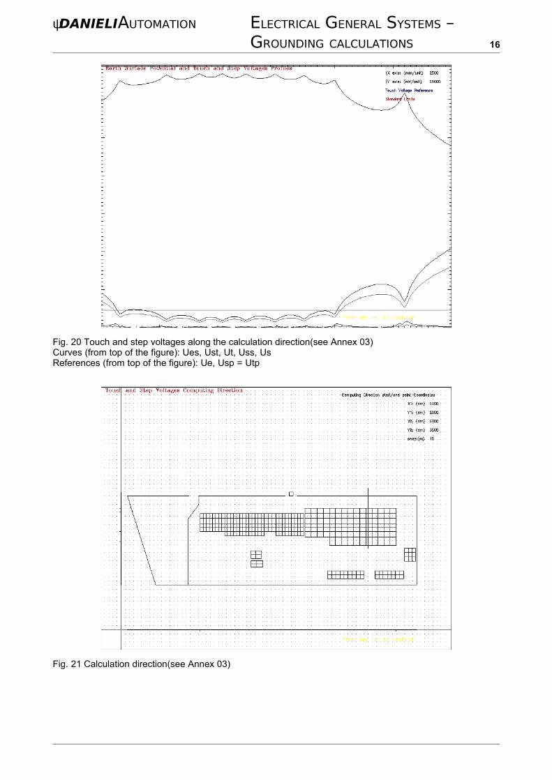
Fig. 20 Touch and step voltages along the calculation direction(see Annex 03)Curves (from top of the figure): Ues, Ust, Ut, Uss, UsReferences (from top of the figure): Ue, Usp = Utp
Fig. 21 Calculation direction(see Annex 03)
ψDANIELIAUTOMATION ELECTRICAL GENERAL SYSTEMS – GROUNDING CALCULATIONS 17
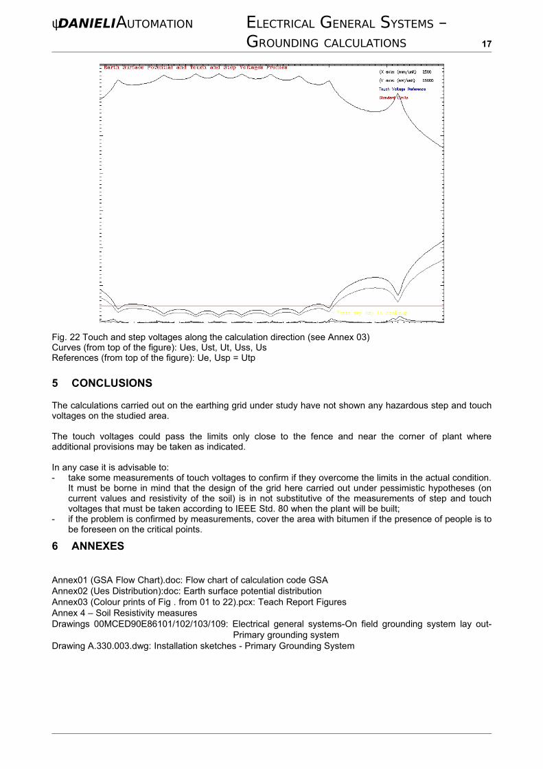
Fig. 22 Touch and step voltages along the calculation direction (see Annex 03)Curves (from top of the figure): Ues, Ust, Ut, Uss, UsReferences (from top of the figure): Ue, Usp = Utp
5 CONCLUSIONS
The calculations carried out on the earthing grid under study have not shown any hazardous step and touch voltages on the studied area.
The touch voltages could pass the limits only close to the fence and near the corner of plant where additional provisions may be taken as indicated.
In any case it is advisable to:- take some measurements of touch voltages to confirm if they overcome the limits in the actual condition.
It must be borne in mind that the design of the grid here carried out under pessimistic hypotheses (on current values and resistivity of the soil) is in not substitutive of the measurements of step and touch voltages that must be taken according to IEEE Std. 80 when the plant will be built;
- if the problem is confirmed by measurements, cover the area with bitumen if the presence of people is to be foreseen on the critical points.
6 ANNEXES
Annex01 (GSA Flow Chart).doc: Flow chart of calculation code GSAAnnex02 (Ues Distribution):doc: Earth surface potential distributionAnnex03 (Colour prints of Fig . from 01 to 22).pcx: Teach Report FiguresAnnex 4 – Soil Resistivity measuresDrawings 00MCED90E86101/102/103/109: Electrical general systems-On field grounding system lay out-
Primary grounding systemDrawing A.330.003.dwg: Installation sketches - Primary Grounding System