
Dobesch Rpt
123
BASIC METEOROLOGICAL CONCEPTS AND RECOMMENDATIONS FOR THE EXPLOITATION OF WIND ENERGY IN THE ATMOSPHERIC BOUNDARY LAYER by Hartwig Dobesch Central Institute for Meteorology and Geodynamics (ZAMG) Vienna, Austria and Georg Kury ENAIRGY Vienna, Austria
-
Upload
francesco-castellani -
Category
Documents
-
view
232 -
download
0
Transcript of Dobesch Rpt
8/2/2019 Dobesch Rpt
http://slidepdf.com/reader/full/dobesch-rpt 1/123
BASIC METEOROLOGICAL CONCEPTS AND
RECOMMENDATIONS FOR THE EXPLOITATIONOF WIND ENERGY IN THEATMOSPHERIC BOUNDARY LAYER
by
Hartwig Dobesch
Central Institute for Meteorology and Geodynamics (ZAMG)
Vienna, Austria
and
Georg Kury
ENAIRGY
Vienna, Austria

8/2/2019 Dobesch Rpt
http://slidepdf.com/reader/full/dobesch-rpt 2/123

8/2/2019 Dobesch Rpt
http://slidepdf.com/reader/full/dobesch-rpt 3/123
i
TABLE OF CONTENTS
FOREWORD....................................................................................................................................................iv
Acknowledgement ............................................................................................................................................iv
1 INTRODUCTION......................................................................................................................................1
1.1 Facts about world energy consumption ..................................................................................................1
1.2 The global situation in the use of wind energy - overview.....................................................................1
1.3 Historical background of wind power usage up to the second oil crisis in 1980....................................2
1.3.1 Wind wheels with vertical axis ...........................................................................................................31.3.2 Wind wheels with horizontal axis .......................................................................................................3
1.4 Development in wind energy technologies and markets since 1973 ......................................................4
2 SOME TECHNICAL ASPECTS OF WIND ENERGY UTILISATION ..................................................7
2.1 The power of a moving air mass.............................................................................................................7
2.2 The power of an ideal WEC....................................................................................................................8
2.3 Aerodynamic concepts for power extraction ........................................................................................10
2.3.1 The aerodynamic drag.......................................................................................................................102.3.2 The aerodynamic buoyancy...............................................................................................................12
2.4 Conversion of kinetic energy into other energy forms..........................................................................17
2.4.1 Heat ...................................................................................................................................................172.4.2 Potential energy.................................................................................................................................17
2.4.3 Electric energy...................................................................................................................................182.5 Power curves of real wind turbines.......................................................................................................19
2.6 Control systems and yaw drives of WECs............................................................................................21
2.7 Technical availability and life span of WECs.......................................................................................21
3 METEOROLOGICAL PARAMETERS IMPORTANT FOR THE SITING PROCEDURE AND THELIFE SPAN OF WECS....................................................................................................................................23
3.1 The air density.......................................................................................................................................233.1.1 Definition ..........................................................................................................................................233.1.2 The height dependency of the air density..........................................................................................24
3.1.3 The effects of air density on the energy yield of WECs....................................................................253.2 The spatial distribution of the wind vector ...........................................................................................263.2.1 Large-scale wind flows .....................................................................................................................263.2.2 Small-scale wind systems..................................................................................................................28
3.3 The temporal variation of the wind vector............................................................................................29
3.4 The influence of precipitation events....................................................................................................343.4.1 Heavy rain .........................................................................................................................................343.4.2 Hail353.4.3 Icing...................................................................................................................................................35
3.5 Lightning strikes ...................................................................................................................................38
4 SPATIAL DISTRIBUTION OF THE WIND SPEED ABOVE HOMOGENEOUS TERRAIN ............41
4.1 The atmospheric boundary layer...........................................................................................................41
8/2/2019 Dobesch Rpt
http://slidepdf.com/reader/full/dobesch-rpt 4/123
ii
4.2 The basic governing equations of the ABL.......................................................................................... 424.2.1 The ideal gas law ..............................................................................................................................424.2.2 Conservation of mass........................................................................................................................424.2.3 Conservation of momentum.............................................................................................................. 424.2.4 Conservation of moisture and the first law of thermodynamics ....................................................... 434.2.5 The equations in simplified form...................................................................................................... 434.2.6 The Reynold’s shear stress and the friction velocity ........................................................................ 444.2.7 The Boussinesq approximation.........................................................................................................45
4.3 The vertical profile of the wind speed in adiabatic stratification ......................................................... 464.3.1 The K-theory and the concept of the mixing-length ......................................................................... 464.3.2 The logarithmic wind profile ............................................................................................................ 474.3.3 The power law...................................................................................................................................48
4.4 The roughness length and its estimation...............................................................................................48
4.4.1 Estimation of the roughness length from measurements at two heights ........................................... 494.4.2 Estimation of the roughness length by means of terrain classification............................................. 49
4.4.3 Estimation of the roughness length from the gustiness.....................................................................514.4.4 Estimation of the roughness length from properties of the earth’s surface.......................................51
4.5 The vertical wind profile in non-adiabatic stratification ...................................................................... 55
4.5.1 The Monin-Obuchov length..............................................................................................................554.5.2 The vertical profile of wind speed in stable stratification................................................................. 554.5.3 The vertical profile of the wind speed in unstable stratification ....................................................... 564.5.4 The concept of the internal boundary layer.......................................................................................564.5.5 Comparison of extrapolation procedures to hub-height from a lower level ..................................... 57
4.6 The representativeness of wind measurements..................................................................................... 584.6.1 Exposure correction method for wind measurements....................................................................... 59
5 FLOW FIELDS AND OROGRAPHY..................................................................................................... 61
5.1 Flows over and around hills.................................................................................................................. 615.1.1 The Brunt-Väisälä frequency and the atmospheric wavelength........................................................ 615.1.2 Wave regimes of flows over hills ..................................................................................................... 625.1.3 Non-linear effects of mountain flows ...............................................................................................655.1.4 Overflow of hills with neutral stratification...................................................................................... 68
5.2 Thermally induced flows...................................................................................................................... 775.2.1 Hillside winds ................................................................................................................................... 775.2.2 Valley and mountain winds............................................................................................................... 79
6 MODELLING OF WIND FIELDS.......................................................................................................... 816.1 Introductory remarks ............................................................................................................................ 81
6.2 Mass-consistent models with variational-analytical base..................................................................... 82
6.3 The European Wind Atlas (WAsP ) ....................................................................................................... 84
6.3.1 The obstacle model ........................................................................................................................... 856.3.2 The roughness model ........................................................................................................................ 866.3.3 The orographic model.......................................................................................................................86
6.4 The GESIMA model............................................................................................................................. 87
6.5 Model comparison ................................................................................................................................ 88
7 SITING AND ENERGY YIELD............................................................................................................. 89
7.1 The importance and requirements of siting .......................................................................................... 897.1.1 General considerations......................................................................................................................89
8/2/2019 Dobesch Rpt
http://slidepdf.com/reader/full/dobesch-rpt 5/123
iii
7.1.2 Meteorological data...........................................................................................................................907.1.3 Some aspects of predicting the wind resource on land and offshore ......................................................91
7.2 Estimation of energy yield....................................................................................................................91
7.3 Verification ...........................................................................................................................................94
7.4 Wind farms............................................................................................................................................957.4.1 Energy Loss from the wake effect.....................................................................................................957.4.2 Experiences with wind farms (on- and offshore)...............................................................................98
8 ENVIRONMENTAL IMPACT OF WECS .............................................................................................99
8.1 Sound emission from wind turbines......................................................................................................99
8.2 Shadow casting from wind turbines....................................................................................................1018.2.1 Basic considerations........................................................................................................................1018.2.2 Geometrical data of WECs..............................................................................................................1038.2.3 Distances for the shadow casting ....................................................................................................103
8.2.4 Distances on the basis of the masking of the sun disk by the rotor blades......................................1048.3 Visual intrusion in the landscape ........................................................................................................104
8.4 Electromagnetic interference ..............................................................................................................105
8.5 Résumé................................................................................................................................................105
9 REFERENCES.......................................................................................................................................107
ANNEX .........................................................................................................................................................114
List of Figures................................................................................................................................................114
List of Tables .................................................................................................................................................116
Symbols .........................................................................................................................................................117

8/2/2019 Dobesch Rpt
http://slidepdf.com/reader/full/dobesch-rpt 6/123
iv
FOREWORD
In 1981 the secretariat of the World Meteorological Organisation edited the Technical Note No. 175,
(WMO – No. 575) “Meteorological Aspects of the Utilisation of Wind as an Energy Resource“. This
document focused mainly on the description of wind as a renewable energy resource from a meteorological
point of view and on the role of the boundary layer and atmospheric turbulence for wind fields. Compiledaround 1980, this Technical Note was edited at the beginning of the stormy development of wind power
exploitation taking place in Europe. Therefore little can be found find on wind energy technology, the
assessment of wind energy potentials and the estimation of energy yield at given sites. This is not surprising
given the remarkable development of methods and technology over the last twenty years. A recently edited
WMO report ("Meteorological Aspects and recommendations for Assessing and Using the Wind as an
energy source in the Tropics", WMO/TD-No. 826, June 1997) contains guidelines for prospecting wind
energy in the tropics, particularly for the numerous islands in this region. Based on experiences made in
Hawaii, this report can be seen as a complimentary document to the above mentioned WMO report No. 575
for those who plan to conduct wind energy surveys in tropical areas. It contains many details and hints under
consideration of the unique tropical weather conditions, compiled and presented for direct practical use but
lacking the physical background in hydrodynamics necessary for example to asses wind energy yield.
This new report will therefore try to fill the gaps in the contents of the above mentioned reports,
from the knowledge base now available at the very beginning of the third millennium. It will reflect the
scope of modern wind technology and its close connection with meteorology, to provide a coherent
presentation of the fundamental aspects of wind energy exploitation and the technical and physical
background. It will emphasise the technical solutions available in the existing area of knowledge and the part
of meteorology, in particular the mathematical-physical bases for the assessment of wind energy potentials,
the optimal siting together with the evaluation of the energy yield of Wind Energy Converters (abbreviated
in the following text as WECs) - beside all practical and theoretical aspects reflected in many textbooks and
reports (e.g. in Petersen et al., 1998) that already contain a realm of wisdom.
Acknowledgement
The authors thank herewith Ms. Jean Palutikof, University of East Anglia, Norwich, for her engagement in
reading carefully and editing this report and for her valuable contribution regarding off-shore wind farms.

8/2/2019 Dobesch Rpt
http://slidepdf.com/reader/full/dobesch-rpt 7/123
1
1 INTRODUCTION
A range of environmental impacts and resource problems have always emerged from the use of
energy technology. For modern societies the supply and sources of energy in their many forms have been an
essential source of economic and political tensions. Together with environmental problems arising from
energy consumption (increase of carbon dioxide and greenhouse effect, acid rain, radioactive waste, oilpollution of the sea), the problems of sustainability and potential social conflict which may result from
unevenly distributed resources, vulnerability due to centralisation and dangers from nuclear proliferation,
make it imperative for mankind to devise a set of energy technologies, which can meet human needs without
producing irreversible environmental effects on a global scale (Elliott, 1997). This implies beside the
requirement to use energy more efficiently, the promotion of technologies that use renewable energy
resources extensively needs to be encouraged.
1.1 Facts about world energy consumption
In the 20 years from 1970-89 world energy consumption rose by about 53 percent from 2.14x10²⁰ J
to 3.28x10²⁰
J. The consumption of fossil fuel energy climbed by 49.2 percent from 2.09x10²⁰
J to 3.12
x1020
J and that of nuclear energy by 2270 percent from 9.83 x10¹⁶
J to 2.33 x10¹⁸
J.
In the seventies of the 20th century people worried about a coming shortage of energy resources and
the direct consequences for the environment e.g. acid rain. From the 1980's, the indirect consequences of
high energy consumption e.g. global warming and the ozone hole, became a greater concern.
The outlook for future energy demand is that it is predicted to rise quite dramatically. It is supposed
(International Energy Agency, 1998; Greenpeace, 1999) that from 1998 to 2010 the world-wide yearly
electricity demand will rise by about 30 percent to 20,852 TWh and by nearly 50 percent to 27,326 TWh by
2020, with an average annual growth rate of 2 percent. Until 2025, the consumption of the developingcountries is estimated to rise on the basis of population growth and increasing industrialisation by more than
100 percent, followed by the former Soviet Union and Eastern Europe with an increase of about 80 percent.
Although the share of fossil fuels used in the production sector will shrink remarkably, the CO2 emissions
will increase by about 50 percent due to overall rising consumption.
The aforementioned risk to the biosphere and the limit on fossil fuel energy resources will force new
solutions. One of the best solutions on the basis of today's technologies, consists of a combination of saving
energy by different measures and the exploitation of additional sustainable resources of energy such as solar
energy (photovoltaic, heat collectors) and wind energy.
1.2 The global situation in the use of wind energy - overview
Wind energy is the kinetic energy content of a moving air mass. The kinetic energy content of the
global atmosphere equals on average a turnover time of about seven days of kinetic energy production or
dissipation, also assuming average rates (Sørensen, 2000). The annual streaming energy of the atmosphere
lies between 8.2 and 13.6 x10²²
J. The entire electricity demand of the earth in 1990 could have been covered
by the use of only 0.04 percent of this energy. The world’s total onshore wind resources (without Antarctica,
Greenland) are estimated to be about 53,000 TWh with the following distribution (M. Grubb and N. I.
Meyer, 1993): Western Europe 4,800 TWh (UK has here the largest share with 986 TWh/a which covers 307
percent of the electricity consumtion), Eastern Europe and former Soviet Union 10,600 TWh, Rest of Asia
4.600 TWh, Latin America 5,400 TWh, North America 14,000 TWh, Australia 3,000 TWh and Africa10,500 TWh.
8/2/2019 Dobesch Rpt
http://slidepdf.com/reader/full/dobesch-rpt 8/123
2
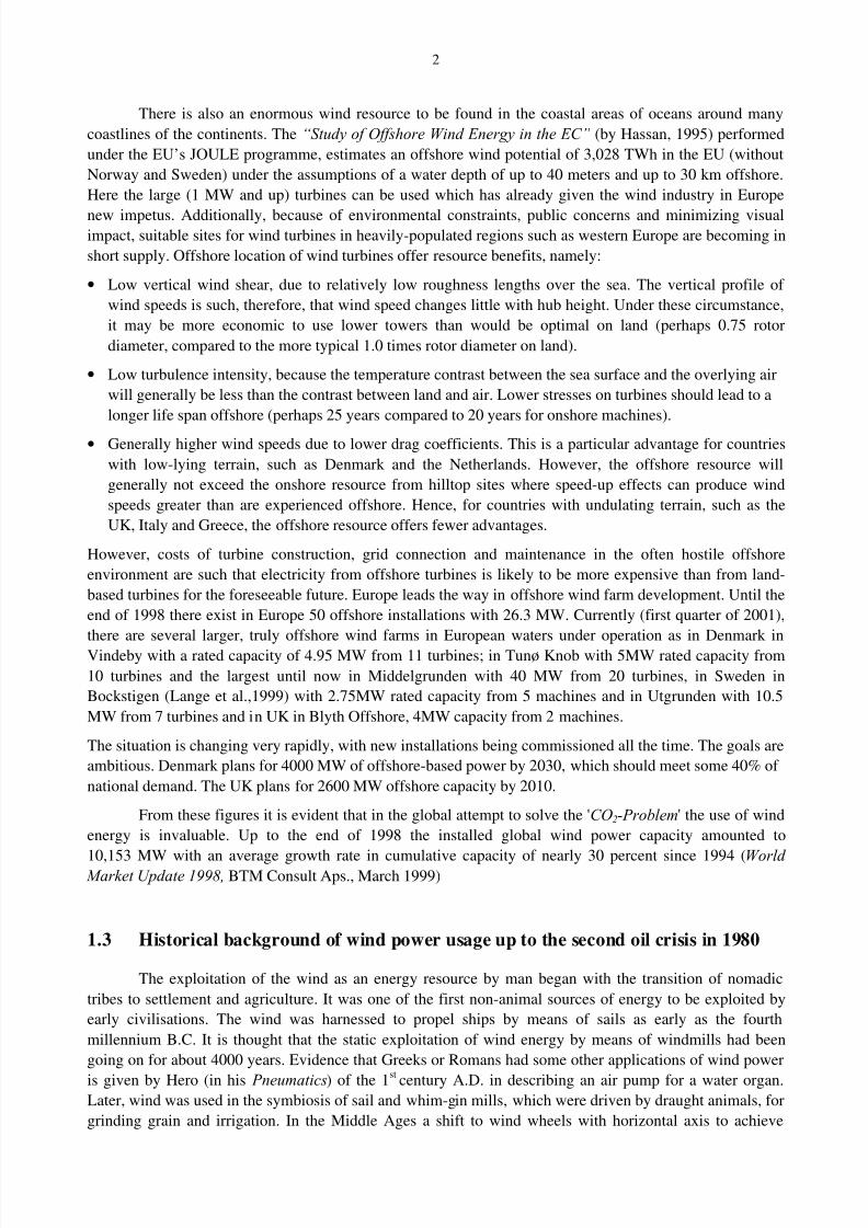
There is also an enormous wind resource to be found in the coastal areas of oceans around many
coastlines of the continents. The “Study of Offshore Wind Energy in the EC” (by Hassan, 1995) performed
under the EU’s JOULE programme, estimates an offshore wind potential of 3,028 TWh in the EU (without
Norway and Sweden) under the assumptions of a water depth of up to 40 meters and up to 30 km offshore.
Here the large (1 MW and up) turbines can be used which has already given the wind industry in Europe
new impetus. Additionally, because of environmental constraints, public concerns and minimizing visualimpact, suitable sites for wind turbines in heavily-populated regions such as western Europe are becoming in
short supply. Offshore location of wind turbines offer resource benefits, namely:
• Low vertical wind shear, due to relatively low roughness lengths over the sea. The vertical profile of
wind speeds is such, therefore, that wind speed changes little with hub height. Under these circumstance,
it may be more economic to use lower towers than would be optimal on land (perhaps 0.75 rotor
diameter, compared to the more typical 1.0 times rotor diameter on land).
• Low turbulence intensity, because the temperature contrast between the sea surface and the overlying air
will generally be less than the contrast between land and air. Lower stresses on turbines should lead to a
longer life span offshore (perhaps 25 years compared to 20 years for onshore machines).
• Generally higher wind speeds due to lower drag coefficients. This is a particular advantage for countries
with low-lying terrain, such as Denmark and the Netherlands. However, the offshore resource will
generally not exceed the onshore resource from hilltop sites where speed-up effects can produce wind
speeds greater than are experienced offshore. Hence, for countries with undulating terrain, such as the
UK, Italy and Greece, the offshore resource offers fewer advantages.
However, costs of turbine construction, grid connection and maintenance in the often hostile offshore
environment are such that electricity from offshore turbines is likely to be more expensive than from land-
based turbines for the foreseeable future. Europe leads the way in offshore wind farm development. Until the
end of 1998 there exist in Europe 50 offshore installations with 26.3 MW. Currently (first quarter of 2001),
there are several larger, truly offshore wind farms in European waters under operation as in Denmark in
Vindeby with a rated capacity of 4.95 MW from 11 turbines; in Tunø Knob with 5MW rated capacity from
10 turbines and the largest until now in Middelgrunden with 40 MW from 20 turbines, in Sweden in
Bockstigen (Lange et al.,1999) with 2.75MW rated capacity from 5 machines and in Utgrunden with 10.5
MW from 7 turbines and in UK in Blyth Offshore, 4MW capacity from 2 machines.
The situation is changing very rapidly, with new installations being commissioned all the time. The goals are
ambitious. Denmark plans for 4000 MW of offshore-based power by 2030, which should meet some 40% of
national demand. The UK plans for 2600 MW offshore capacity by 2010.
From these figures it is evident that in the global attempt to solve the 'CO2-Problem' the use of wind
energy is invaluable. Up to the end of 1998 the installed global wind power capacity amounted to
10,153 MW with an average growth rate in cumulative capacity of nearly 30 percent since 1994 (World Market Update 1998, BTM Consult Aps., March 1999)
1.3 Historical background of wind power usage up to the second oil crisis in 1980
The exploitation of the wind as an energy resource by man began with the transition of nomadic
tribes to settlement and agriculture. It was one of the first non-animal sources of energy to be exploited by
early civilisations. The wind was harnessed to propel ships by means of sails as early as the fourth
millennium B.C. It is thought that the static exploitation of wind energy by means of windmills had been
going on for about 4000 years. Evidence that Greeks or Romans had some other applications of wind power
is given by Hero (in his Pneumatics) of the 1st century A.D. in describing an air pump for a water organ.Later, wind was used in the symbiosis of sail and whim-gin mills, which were driven by draught animals, for
grinding grain and irrigation. In the Middle Ages a shift to wind wheels with horizontal axis to achieve
8/2/2019 Dobesch Rpt
http://slidepdf.com/reader/full/dobesch-rpt 9/123
3
higher efficiency occurred, though mainly in areas where hydraulic power was unavailable. With increasing
industrialisation at the beginning of the 18th
century more and more fossil energy was used thus replacing
slowly regenerative energy, until finally at the end of the 19th
century the fossil fuels overtook regenerative
energy use (the trade statistics of the German empire 1895 provide the following figures: 18,362 wind
machines, 21,350 combustion engines, 54,529 water machines and 58,530 steam engines (Gasch, 1991). The
20th
century cared little for wind energy until a renaissance in the 70’s and 80’s as a consequence of oil crisisand ecology movements.
1.3.1 Wind wheels with vertical axis
Wind wheels with vertical axis are based usually on the resistance principle, which was already
known by early civilisations as power sources. Early evidence of a simple windmill was found in Egypt and
Mesopotamia 1000 B.C. where they were used for irrigation. Another early occurrence is reported from
Afghanistan in the 7th
century. All these early power plants were constructed around the following
mechanism: In a half open tower a turntable with resistance surfaces from round timbers or woven mats was
established, which was rotated by one-sided upwind. The disadvantage of this arrangement was itsdirectional dependence. This was initially overcome by the Chinese around 1000 A.D. by turning the sail-
mats out of the wind on their return travel against the wind. Another solution Veranzio discovered in Italy
around 1600 by generating a torque in asymmetric wind flow: He used resistance bodies, which had,
according to the direction of flow, larger or smaller drag-coefficients – which employs the same principle as
the cup anemometer (Gasch,1991).
Through the striking success of the horizontal axis rotors the vertical axis principle experienced no
improvement until 1924 when the SAVONIUS rotor, named after its Finnish inventor, was introduced. By
the use of the buoyancy principle, a higher efficiency is attainable with this WEC. A further design step in
competition to the horizontal axis is the DARRIEUS rotor. Developed by the French inventor Darrieus in
1929, this rotor can reach an efficiency of 38 percent after steered start up to the rated-speed range(Molly,1990).
1.3.2 Wind wheels with horizontal axis
The vertical axis turbines that exploit an effect sailors had discovered early on, i.e. sail ships travel
faster if the wind comes from the side instead of behind, spread slowly. The physical explanation for this lay
in the use of dynamic buoyancy where much greater power can be generated than with the aerodynamic
resistance principle. The first windmills using this principle consisted of up to ten wooden booms, rigged
with jib sails. Such primitive types of windmills are still found today in the eastern Mediterranean regions
(sail windmills in Greece). The concept of this 'propeller' windmills arrived in England and France withreturning crusaders, where it appeared in the 12
thcentury in the form of the buck-windmill, spreading from
there to Holland and Germany in the 13th century, and thence Poland and Russia in the 14th century. During
the subsequent Middle Ages most manorial rights included the right to refuse permission to build windmills,
thus compelling tenants to have their grain ground at the mill of the lord of the manor. Additionally, planting
of trees near windmills was banned to ensure free wind (DeRenzo, 1979). The oldest construction was the
so-called “post-mill” in which the whole body of the mill was moved around a large upright post when the
wind direction changed. This mill had to be brought into the wind by the miller or a donkey. The
disadvantage of the post-mill was that heavy loads like millstones and grain sacks had to be carried into the
mill house and that it could not be used for the drainage of the countryside for which a high demand had
long existed in Holland. A further development of this type of mill took place 300 years later in the form of
the Wippmill which could be used for water pumping. The disadvantage remained that the entire mill neededturning manually into the wind (Gasch 1991).
8/2/2019 Dobesch Rpt
http://slidepdf.com/reader/full/dobesch-rpt 10/123
8/2/2019 Dobesch Rpt
http://slidepdf.com/reader/full/dobesch-rpt 11/123
5
perimeter with flaps for the power regulation, similar to these used in the aeroplane construction. As a result
of the flaps a contortion of the entire rotor could be avoided, allowing the two rotor blades to be
manufactured in one piece and installed on a commuting hub. Due to technical problems non of these three
prototypes reached series maturity (Hau, 1996; Thomas, 1976; Gasch 1991).
The construction of vertical-axis turbines was further developed in Canada: 1988 a DARRIEUS
rotor with 4.2 MW power was installed that holds the world record in generator performance since then and,
additionally, reached a high technical availability (95 percent) in the first two years of operation. Because of
the high cost this development was not followed up until now . Also in Sweden megawatt generators with a
relatively high technical availability were installed. The first Swedish prototype was the MAGLARP WTS 3
with 78 meter rotor diameter and 3 MW performance, followed by the two AEOLUS plants, AEOLUS I
with 2 MW and a rotor diameter of 75 meters and AEOLUS II with 3 MW and 80 meter rotor diameter
(Molly, 1990). In Germany of the 1980's, starting from the 100 KW HUETTER machine with a rocking
suspension of a two-bladed rotor in the lee of the tower, a 3 MW turbine with 100 meter rotor diameter and
100 meters hub height was erected. This generator was named GROWIAN (= “Große Wind Anlage”) and
completed only 420 hours in operation due to material fatigue of some components of the rotor teetering hub
and was demolished in spring 1988. In 1989 with the MONOPTEROS 50 the first larger single blade turbinewith a rotor diameter of 56 meters and a nominal power of 640 KW was erected. The goal of this
development was to lower the costs by reducing material expenditure for the rotor blade and by decreasing
the translation of the gear (single- bladed rotors can reach essentially higher speeds as two- or three-blade
rotors). However, with increasing speed of the blade tips the noise emission increases to the 5 th power of
speed, single-bladed rotors could not succeed. Another megawatt plant followed in 1990 with the WKA60 of
60 meters diameter and 1200 KW power, however none of these had any effects on the current WEC market
(Hau, 1996; Molly, 1990; Gasch, 1991).
In Nordjütland, Denmark, two medium-sized installations „NIBE A “and „NIBE B“ were
constructed in 1979 and 1980. Their design was based on the GEDSER turbine, erected in 1957. They both
had 40 meter rotor diameters and 630 KW power, but differed in the control mechanism: one unit couldchange the angle of attack of the entire rotor blade, the other unit could only vary the angle of attack of the
blade tips in two positions. This blade tip regulation is in fact cheaper, but produced less energy yield.
However, a comparison of both systems did not lead to a preference to one of either construction principle
(Molly, 1990).
As early as 1977 on a private initiative of students in Denmark a 2 MW plant, the TVIND mill, with
a 54 meter rotor diameter was built. It provided a pronounced impetus for the Danish anti-nuclear
movement. But only considerably later, in 1988, was another 2 MW plant, the ELSAM-2000 with 61 meter
rotor diameter installed, funded by the Danish government. At the end of the 1970's from small - and
medium sized enterprises smaller units with up to 15 meter rotor diameter were developed for private
operators, all based on the principle of the GEDSER design: This principle known under the name „Danish
concept“ marks WECs with horizontal axis, wind-ward side rotor with three GFK-blades on a stiff hub and
with constant rotational speed propelling a network-connected asynchronous generator. The drive train
consists of standard components (gear, brake, clutch, generator) in linear order on a machine bearer. The
windward orientation takes place with a yaw motor, the power restriction by flow separation at the rotor
blades and the protection against high winds by mechanical and aerodynamic brakes (Gasch, 1991). A more
extended overview of the above outlined development is given for example in Quarton et al. (1998).
In the past and presently different market regulation, market stimulation and development incentives
are offered by governments as political initiatives to promote wind energy usage. Thus the Federal Public
Utility Regulatory Policies Act (PURPA) of the U.S. Carter-Administration, passed in 1978, led especially in
California to the development of a market, where a guarantee was given for independently produced
electricity, providing favourable regulation for feeding into the grid and fiscal relief for the operating of
WECs. From 1982 Danish companies, like VESTAS, could install thousands of VESTAS-V15s with
15 meter rotor diameter and 55 KW performance in the Tehachapi Mountains and on the Altamont Pass, the
8/2/2019 Dobesch Rpt
http://slidepdf.com/reader/full/dobesch-rpt 12/123
6
locations of the largest Californian wind farms. The large turbines from the aeronautics industry (Boeing,
MBB, DORNIER) mostly failed due to technical or financial problems, but the Danish WEC manufacturers
had recognised the demands of the market and took on the leading role in the world market: From 18,000
erected WECs in California that were erected until 1990 (total-performance 1500 MW), 45 percent came
from Denmark (Hau, 1996; Gasch, 1991). But after this boom the growth of wind energy in California was
not sustained neither was any development elsewhere in the USA and only in 1997 the US market wasstarting to re-emerge. In contrast, there has been striking developments in Europe markets as in Germany in
the early 1990’s where around 200 MW of wind power were installed per annum. Since shown in a study by
the EC of 1988 that the advantages of a promotion of the operator instead of the manufacturer and
additionally, that more effective plants should get bigger market odds, a support of 0.06 DM per generated
KWh was guaranteed by the 250 MW-Programme (started in 1991) By this buyback policy and other
measures the use of wind energy in Germany boomed, and the annual installation had reached 150 MW in
1993, 309 MW in 1994 and 509 MW in 1995 (Energiewerkstatt, 1993). This increase was due to the
enlargement of the generator performance from 250 to 500/600 KW, and in the following years prototypes
with up to 1500 KW were designed.
Until September 2000 a total global performance of 15,887 MW were installed, Germany leadingwith 5,432 MW (which took the world-wide lead in 1998 from the USA), the USA with 2,495 MW,
followed by Spain with 2,099 MW, Denmark with 2,016 MW and India with 1,094 MW (from NEW
ENERGY No.6, December 2000). From these results it can be seen that wind power has been the energy
success story of the last decade in the 20th century, and particularly in the last two years when it was the
fastest growing energy source of all renewable energy sources.
The future prospects for wind energy exploitation are described in a Greenpeace study (1999) which
was prepared by an independent consulting company (BTM, Denmark). The aim of this study has been to
assess the technical, economic and resource implications for a penetration of wind power into the global
electricity systems equal to 10 percent of total future demand and whether such a 10 percent penetration
might be possible within two decades. In this 10 percent scenario a carbon dioxide reduction due to the useof wind power will amount from 13.3 million tonnes/year in 1998 to 1.780 million tonnes/year in 2020
which gives a cumulative reduction of 10.650 million tonnes/year until 2020.
8/2/2019 Dobesch Rpt
http://slidepdf.com/reader/full/dobesch-rpt 13/123
7
2 SOME TECHNICAL ASPECTS OF WIND ENERGY UTILISATION
Utilising wind energy entails installing a device that converts part of the kinetic energy in the
atmosphere to, say, mechanically useful energy. This kind of conversion of wind energy into the motion of a
body has been in use for a long time. Almost any physical construction that produces an asymmetric force in
a wind flow can be made to rotate, translate or oscillate thereby generating power. How this works is shown
in the next sections.
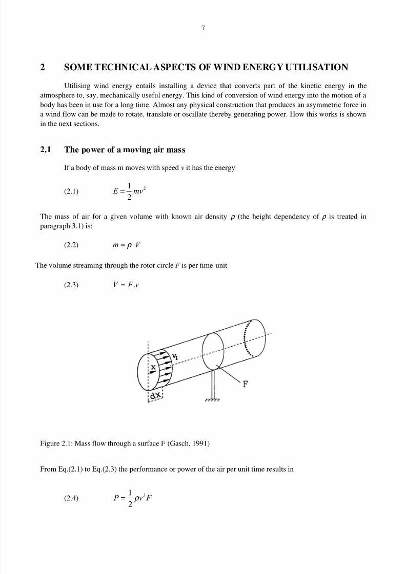
2.1 The power of a moving air mass
If a body of mass m moves with speed v it has the energy
(2.1) E mv=1
2
2
The mass of air for a given volume with known air density ρ (the height dependency of ρ is treated in
paragraph 3.1) is:
(2.2) m V = ⋅ρ
The volume streaming through the rotor circle F is per time-unit
(2.3) v F V .=
Figure 2.1: Mass flow through a surface F (Gasch, 1991)
From Eq.(2.1) to Eq.(2.3) the performance or power of the air per unit time results in
(2.4) F v P 3
2
1ρ =
8/2/2019 Dobesch Rpt
http://slidepdf.com/reader/full/dobesch-rpt 14/123
8
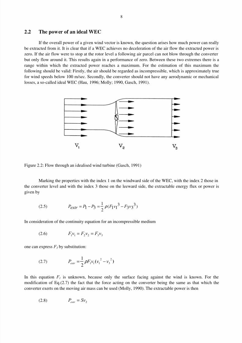
2.2 The power of an ideal WEC
If the overall power of a given wind vector is known, the question arises how much power can really
be extracted from it. It is clear that if a WEC achieves no deceleration of the air flow the extracted power is
zero. If the air flow were to stop at the rotor level a following air parcel can not blow through the converter
but only flow around it. This results again in a performance of zero. Between these two extremes there is arange within which the extracted power reaches a maximum. For the estimation of this maximum the
following should be valid: Firstly, the air should be regarded as incompressible, which is approximately true
for wind speeds below 100 m/sec. Secondly, the converter should not have any aerodynamic or mechanical
losses, a so-called ideal WEC (Hau, 1996; Molly; 1990, Gasch, 1991).
Figure 2.2: Flow through an idealised wind turbine (Gasch, 1991)
Marking the properties with the index 1 on the windward side of the WEC, with the index 2 those inthe converter level and with the index 3 those on the leeward side, the extractable energy flux or power is
given by
(2.5) )333
311(
2
131 v F v F P P extr P −=−= ρ
In consideration of the continuity equation for an incompressible medium
(2.6) 332211 v F v F v F ==
one can express F 3 by substitution:
(2.7) )(2
3
2
1112
1vvv F P extr −= ρ
In this equation F 1 is unknown, because only the surface facing against the wind is known. For the
modification of Eq.(2.7) the fact that the force acting on the converter being the same as that which the
converter exerts on the moving air mass can be used (Molly, 1990). The extractable power is then
(2.8) 2Sv P extr =

8/2/2019 Dobesch Rpt
http://slidepdf.com/reader/full/dobesch-rpt 15/123
9
with
(2.9) )()(.
311131 vvv F vvmS −=−= ρ
Setting Eq.(2.7) equal to Eq.(2.9) it follows
(2.10) )( 3122
1vvv += ,
which is known as the Froude-Rankine’ theorem (Gasch, 1991). Considering Eq.(2.6) the extractable power
results as:
(2.11) ))((2
3
2
13124
1vvvv F P extr −+= ρ
Dividing Eq.(2.11) by the power
(2.12)3
122
1v F P ρ =
the rate of effective extractable power of the WEC, called the power-coefficient, yields
(2.13) ))(( x x P
P c extr
p +−== 112
1 2,
with x = v3 /v1. In order to determine the maximum of c p, the first derivation of c p with respect to x must be
set to zero and then x determined from this, introducing this result into Eq.(2.13) we get the so-called
maximum power-coefficient:
(2.14 a) 5926027
16.max == pc
(2.14 b) 13
3
1vv opt =
(2.14 c) 123
2vv opt =

8/2/2019 Dobesch Rpt
http://slidepdf.com/reader/full/dobesch-rpt 16/123
10
Figure 2.3: The course of the power-coefficient with respect to the ratio of the velocities in front andbehind a rotor, x = v3 /v1 (Hau, 1996)
The maximum power density that can be extracted by a WEC from the wind flow will be
consequently at a maximum at 59.26 percent (Figure 2.3) of the actual given wind power. For comparison
caloric power plants have only an efficiency of about 30 to 40 percent.
2.3 Aerodynamic concepts for power extraction
2.3.1 The aerodynamic drag
The utilisation of the aerodynamic drag represents the oldest form of extracting power from the
wind. Each surface F , standing vertically in the flow, experiences a force which is equal to the drag of the
surface opposite to that flow and which acts in the flow direction (Molly, 1990; Gasch, 1991). This force is
proportional to F , to the air density and to the square of the wind speed:
(2.15)2
2 FvcW w
ρ =
The factor cw is called the drag-coefficient and quantifies the effects from the form of the resistance surface.
In Table 2.1 the drag-coefficients of different bodies are listed:
Table 2.1: The drag-coefficients of different bodies (Boeswirth, 1993)
Body cw
Hemispheric cup, open opposite to the current 1.33
Hemispheric cup, with surface, opposite to the current 1.17
Hemispheric cup, with surface 0.40
Circular disk 1.11
Rectangular strip, w : h = 4 1.19

8/2/2019 Dobesch Rpt
http://slidepdf.com/reader/full/dobesch-rpt 17/123
11
For a rotating system of resistance surfaces, which is affected only half-sided by the flow an upwind speed
results with
(2.16) r vuvv wwr ω −=−=
where vw is the wind speed and u the rotation speed of the outer parts of the resistance surface rotating with
the angular velocity ω and an average radius r . For the drag force W it can be written therefore as
(2.17) F uvcW ww
2
2)( −=
ρ
The averaged - in reality slightly pulsating – propulsion power is then
(2.18)
−==
ww
wwv
u
v
uc FvuW P
23
12 )(ρ
and c p
(2.19)ww
w pv
u
v
ucc 21 )( −=
Figure 2.4: Flow conditions and air forces for aerodynamic drag (Hau, 1996)
The ratio u/vw = λ is generally called tip-speed-ratio of the WEC. It is obvious that with converters
based on the aerodynamic drag principle this tip-speed-ratio must lie between zero and one. The optimal
power-coefficient is given with λ =1/3, hence
(2.20) w p cc274=max
8/2/2019 Dobesch Rpt
http://slidepdf.com/reader/full/dobesch-rpt 18/123
12
Assuming a maximum cw = 1.33 (open hemisphere in flow direction), the maximum possible power-
coefficient amounts to c pmax = 0.197. But when considering real machines the surfaces of the covered half-
side experience a drag force proportional to the rotation speed, the power-coefficient is further reduced and it
becomes clearly evident, why this principle plays no current role in the exploitation of wind energy.
2.3.2 The aerodynamic buoyancy
Already by the 18th century power-coefficients from the Dutch Windmills reached 0.28 and present-
day plants have power-coefficients up to c p = 0.5. The principle by which such high efficiencies are reached
is aerodynamic buoyancy. Similar to flow drag it is proportional to the air density, the surface and the square
of the flow velocity. The buoyancy A acts perpendicular to the flow direction (Boeswirth, 1993;
Schlichting, 1967)
(2.21)2
2 Fvc A a
ρ =
ca is named the lift-coefficient and is dependent on the angle of attack α (the angle between the surface of
the rotor plane and the flow direction). For a flat plate thus it is valid:
(2.22) α π α sin)( 2=ac
Most aerodynamically formed profiles from aeroplane design reach higher ca values because they
possess a curvature that reinforces the buoyancy. The drag-coefficients of these profiles compared with the
lift-coefficient are very small: good profiles reach a lift-drag ratio ε εε ε ( = ratio of ca to cw) of over 150. The
point of attack of the force lies for small angles approximately within one third upto a quarter of the blade
depth. The lift-coefficient with larger angles of attack deviates more and more from the theoretical one asgiven by Eq.(2.22). If the angle of attack is larger than a profile-specific threshold that usually lies
approximately around 15 degrees, it decreases with larger angles. The drag increases in this range greatly:
By the strong slanted position of the surface, the flow over the rear can not maintain a regular form, bigger
whirls are formed, leading to a separation of the regular flow from the surface. This condition (see
paragraph.5.1.4) is called flow-separation or stall (Boeswirth, 1993; Schlichting, 1967).
To show the function for the most important group of WECs, (the buoyancy using turbines with
horizontal axis) in the following the distribution of forces on a rotating rotor blade with radius R is
discussed. Firstly, we consider a cross-section of the rotor blade at a distance r from the rotation axis (Gasch,
1991). Because the blade rotates the wind speed is supplemented by the circumference speed to the resulting
upwind speed. How this takes place is shown in Figure 2.5 where the angle of attack ß (with respect to theaxial direction) can be estimated very simply from the tip-speed-ratio:
(2.23) tan β λ =3
2
r
R
8/2/2019 Dobesch Rpt
http://slidepdf.com/reader/full/dobesch-rpt 19/123
13
Figure 2.5: Air forces in the wing path plane (Gasch, 1991)
For this angle the forces can be determined in axis - and in rotation direction. The force in axis direction is
the shear stress dS on the surface, the force dU in the rotation direction causes a power reduction:
(2.24a) dr cccdU wa )sincos( β β ρ
−= 2
2
(2.24b) dr cccdS wa )cossin( β β ρ −= 2
2
Two important results can be derived from this: Firstly, wind turbines based on the buoyancy principle can
reach tip-speed ratios λ > 1. Presently, rotors with high tip-speed ratio reach a λ between 5 and 10. Because
the force of the air depends on the square of the flow speed it is clear why buoyancy using wind turbines
reach essentially higher power-coefficients than aerodynamic drag using types. Secondly, the faster the rotor
blades rotate, the larger the angle ß becomes. Because the lift-coefficient is multiplied by the cosine and the
drag-coefficient by the sine it follows that rotor blades for high rotation speeds must have profiles with a
favourable relationship of ca and cw (Hau, 1996; Molly, 1990).
To reach the optimal range of attenuation of the air in the rotor circle plane (and with it optimalpower extraction), each wing section must have an exactly defined blade shape and angle. Accordingly, if
the spin of the air flowing away is taken into account, or not, one speaks of Schmitz´s or Betz´s design of the
rotor blades. After Schmitz the cord length of a turbine with n rotor blades is
(2.25)nc
r t
a
schmitz
1)
3
1(sin
161
2 α π
= ; with )(tanλ
α r
R1
1−=
8/2/2019 Dobesch Rpt
http://slidepdf.com/reader/full/dobesch-rpt 20/123
14
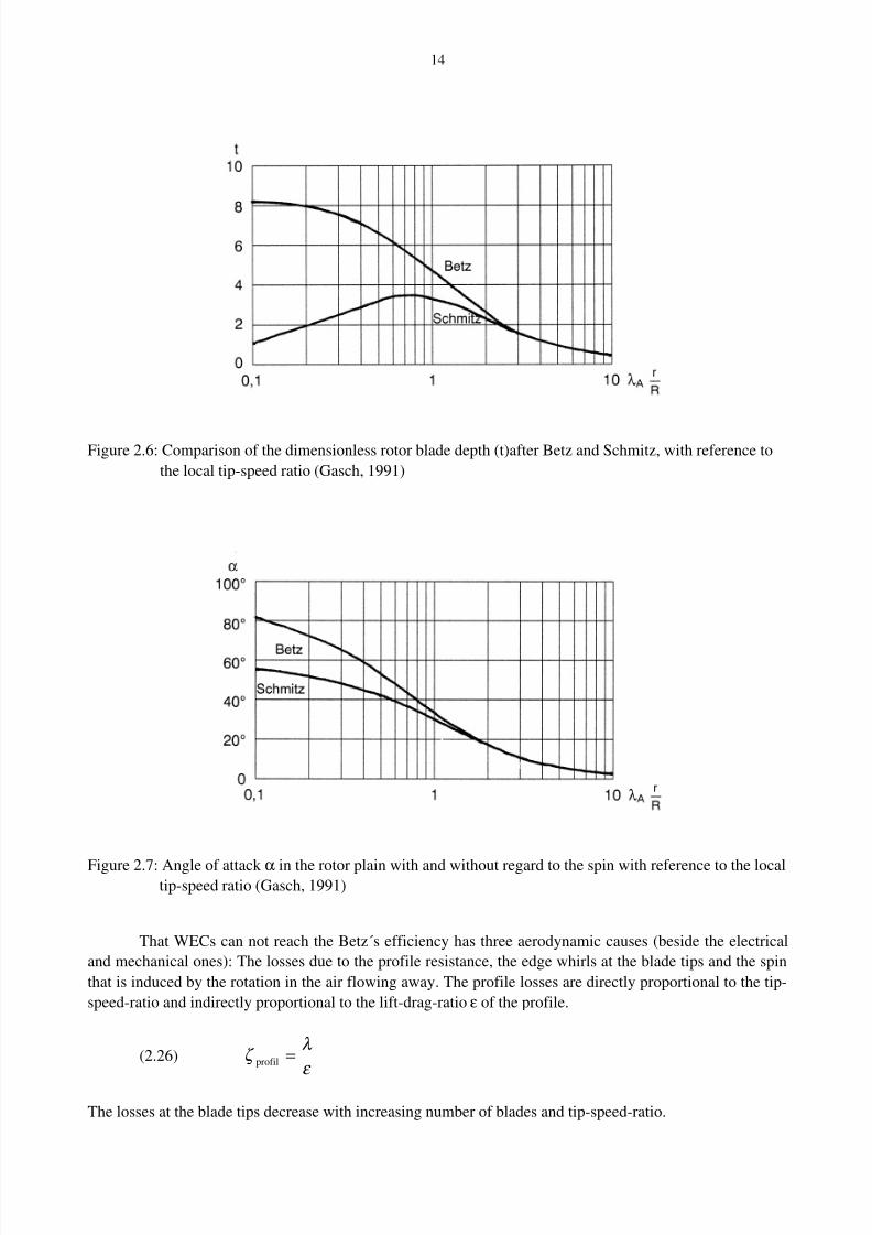
Figure 2.6: Comparison of the dimensionless rotor blade depth (t)after Betz and Schmitz, with reference to
the local tip-speed ratio (Gasch, 1991)
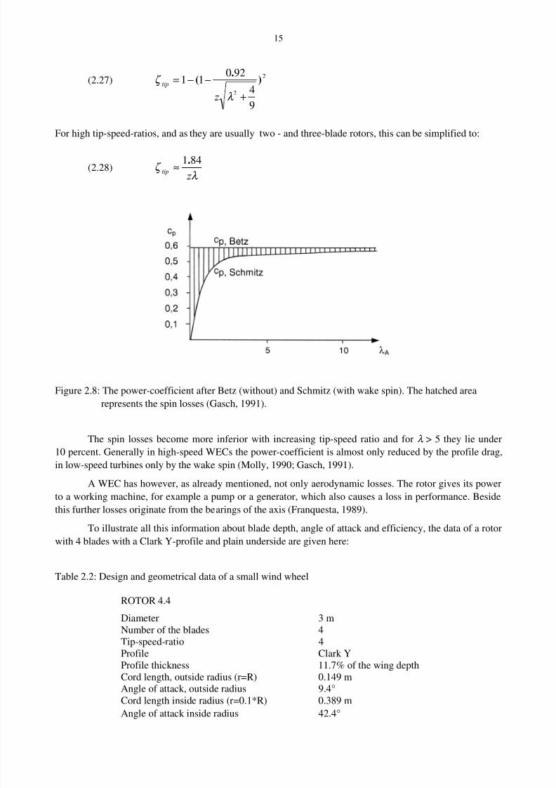
Figure 2.7: Angle of attack α in the rotor plain with and without regard to the spin with reference to the localtip-speed ratio (Gasch, 1991)
That WECs can not reach the Betz´s efficiency has three aerodynamic causes (beside the electrical
and mechanical ones): The losses due to the profile resistance, the edge whirls at the blade tips and the spin
that is induced by the rotation in the air flowing away. The profile losses are directly proportional to the tip-
speed-ratio and indirectly proportional to the lift-drag-ratio ε of the profile.
(2.26) ζ λ
ε profil =
The losses at the blade tips decrease with increasing number of blades and tip-speed-ratio.
8/2/2019 Dobesch Rpt
http://slidepdf.com/reader/full/dobesch-rpt 21/123
15
(2.27)2
2
9
4
92011 )
.(
+−−=
λ
ζ
z
tip
For high tip-speed-ratios, and as they are usually two - and three-blade rotors, this can be simplified to:
(2.28)λ
ζ z
tip
841.≈
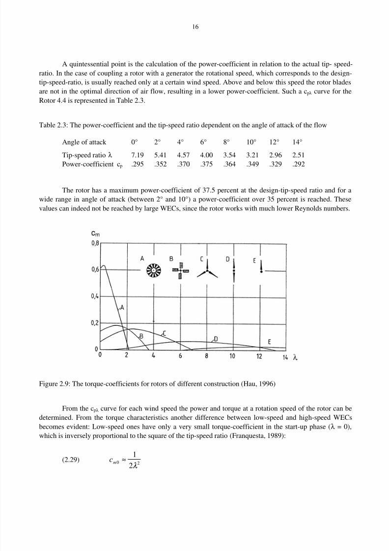
Figure 2.8: The power-coefficient after Betz (without) and Schmitz (with wake spin). The hatched area
represents the spin losses (Gasch, 1991).
The spin losses become more inferior with increasing tip-speed ratio and for λ > 5 they lie under
10 percent. Generally in high-speed WECs the power-coefficient is almost only reduced by the profile drag,
in low-speed turbines only by the wake spin (Molly, 1990; Gasch, 1991).
A WEC has however, as already mentioned, not only aerodynamic losses. The rotor gives its power
to a working machine, for example a pump or a generator, which also causes a loss in performance. Beside
this further losses originate from the bearings of the axis (Franquesta, 1989).
To illustrate all this information about blade depth, angle of attack and efficiency, the data of a rotor
with 4 blades with a Clark Y-profile and plain underside are given here:
Table 2.2: Design and geometrical data of a small wind wheel
ROTOR 4.4
Diameter 3 mNumber of the blades 4Tip-speed-ratio 4Profile Clark YProfile thickness 11.7% of the wing depthCord length, outside radius (r=R) 0.149 m
Angle of attack, outside radius 9.4°Cord length inside radius (r=0.1*R) 0.389 m
Angle of attack inside radius 42.4°
8/2/2019 Dobesch Rpt
http://slidepdf.com/reader/full/dobesch-rpt 22/123
16
A quintessential point is the calculation of the power-coefficient in relation to the actual tip- speed-
ratio. In the case of coupling a rotor with a generator the rotational speed, which corresponds to the design-
tip-speed-ratio, is usually reached only at a certain wind speed. Above and below this speed the rotor blades
are not in the optimal direction of air flow, resulting in a lower power-coefficient. Such a cpλ curve for the
Rotor 4.4 is represented in Table 2.3.
Table 2.3: The power-coefficient and the tip-speed ratio dependent on the angle of attack of the flow
Angle of attack 0° 2° 4° 6° 8° 10° 12° 14°
Tip-speed ratio λ 7.19 5.41 4.57 4.00 3.54 3.21 2.96 2.51
Power-coefficient cp .295 .352 .370 .375 .364 .349 .329 .292
The rotor has a maximum power-coefficient of 37.5 percent at the design-tip-speed ratio and for awide range in angle of attack (between 2° and 10°) a power-coefficient over 35 percent is reached. These
values can indeed not be reached by large WECs, since the rotor works with much lower Reynolds numbers.
Figure 2.9: The torque-coefficients for rotors of different construction (Hau, 1996)
From the cpλ curve for each wind speed the power and torque at a rotation speed of the rotor can be
determined. From the torque characteristics another difference between low-speed and high-speed WECs
becomes evident: Low-speed ones have only a very small torque-coefficient in the start-up phase (λ = 0),
which is inversely proportional to the square of the tip-speed ratio (Franquesta, 1989):
(2.29)20
2
1
λ ≈mc

8/2/2019 Dobesch Rpt
http://slidepdf.com/reader/full/dobesch-rpt 23/123
8/2/2019 Dobesch Rpt
http://slidepdf.com/reader/full/dobesch-rpt 24/123
18
location of the water to be pumped. The hydraulic performance is proportionally to the output M and the
height H (e.g. for pumping) namely:
(2.30) whydr gHM P ρ =
ρ w denotes the density of the water and g the acceleration due to gravity. This means that with the same
power, either small outputs from deep locations (groundwater) or big outputs from near-surface locations
can be achieved.
Which wind generator in which application is used depends on the working machine, in this case the
pump. While piston-pumping using slow up - and downward movement of the plunger can pump water from
up to 300 meters (typical example is the Western Mill ), quickly turning gyroscope pumps can work only over
a height of 10 m.
A disadvantage of the conversion into potential energy is again the linking of the WEC site to the
water occurrences, which is the reason why some wind pump systems use an electrical energy conversion
unit (Gasch, 1991).
2.4.3 Electric energy
The conversion of rotational movement into electricity usually takes place with generators of various
designs. The electrical energy is fed either into the existing electric grid (network-parallel-solution) or,
independently from the grid, is directly used or accumulated in some kind of storage (island-solution).
In the latter case the supply security of the system is of great importance. Because of the strongly
fluctuating wind energy potential large storage capacities must be established to attain a supply security of
100 percent. These storage capacities, in most cases batteries, in rare cases flywheels, are not completely
ecologically harmless in production and raise the costs per generated KWh considerably. Therefore WECs inisland solutions are usually linked with photovoltaic (PV) units, or diesel generators. Island solutions often
work as a wind/diesel combination with constant frequency and with varying generators to a PV/wind
compound system.
In the network-parallel-solution, one distinguishes direct and indirect feeding into the grid: Direct
feeding is allowed if the current of the generator is delivered directly into the grid at constant frequency of
50 Hz ( Europe). Indirect feeding is possible if a direct-current converter exists between generator and grid,
i.e. the generator current is rectified and then reshaped into an alternating current with constant frequency. In
this case a constant frequency at the generator is not necessary and operation with variable rotational speeds
is possible (Molly, 1990).
Advantages of indirect feeding into the grid are the higher aerodynamic efficiency of the rotor,
which can operate over a wide range of design tip-speed-ratios, disadvantages are the additional expenses
and losses due to the frequency conversion technique. Although the number of WECs with indirect feeding
into the grid is increasing recently, still most installations are feeding directly into the grid. Because of the
necessity of an approximately constant rotation speed, which is only reached at a certain wind speed (where
the design-tip-speed-ratio is reached), the unit works in all other speed ranges with poorer efficiency. To
widen the optimal performance range most directly feeding turbines operate as either a high – or a low-wind
speed generator or a pole-changing generator (Hau, 1996).
A variety of designs are used for electrical generators. In smaller WECs mainly for the loading of
accumulators generators with permanent magnets are in use since these can generate electricity even if the
accumulators are completely depleted. Beside the synchronous machines in rarer cases direct-currentgenerators are used, these require no rectifier but have a higher maintenance expenditure (the voltage must
be taken from the collector with slip rings). An important characteristic of generators is the number and
8/2/2019 Dobesch Rpt
http://slidepdf.com/reader/full/dobesch-rpt 25/123
19
order of the poles. When the spool is within the magnet field, one speaks of an external pole generator,
which has the disadvantage that current is collected over wearable slip rings. For internal pole generators
with permanent magnets, or in generators with electromagnets only a low power transfer by slip rings is
necessary. The larger the number of poles the more often the current changes its sign in one revolution. To
attain the grid frequency of 50 Hz with a great number of poles a lower generator speed is required, which
enables the rotor to drive the generator directly without gearing. This gear-less concept is used mostly insmaller units but can be found in large single plants too. The disadvantages are the high weight and cost of
the generator, the advantages are the loss-free transfer of power from the rotor to the generator as well as the
lack of noise pollution and lack of maintenance-intensive rotating parts.
Units with direct grid-feeding have either synchronous or more often asynchronous generators, while
in the indirect grid-feeding units both variants are approximately equally often applied. This can be justified
by the fact that synchronous generators with direct feeding can be disrupted by strong gusts due to the exact
grid synchronisation required, and leads to infringement of the tilting moment which can result in stalling. In
contrast, the asynchronous generator can stand small rotational speed fluctuations, that results in a simpler
grid synchronisation. Furthermore, this kind of generator is simple and inexpensive but its disadvantage is
the need for power to induce the magnetic field that must be taken from the grid or reactance-outputcondensers.
2.5 Power curves of real wind turbines
To forecast the energy yield from a WEC the power curve is used as the technical characteristic for
evaluation of the available power dependent on the wind speed and other relevant meteorological
parameters. Since the working machine, including gears and bearings has a certain resistance against rotation
and as units with high tip-speed-ratio show a low moment-coefficient when still, WECs begin to operate
initially from a certain minimum wind speed, the so-called cut-in wind speed. This speed is defined by the
technical design and is between 3 and 5 m/sec. With increasing wind speed the power output of grid-feeding
WECs show their strongest increase at 1.4 to 2 times the average annual wind speed (Hau, 1996; Franquesta,
1989). The power increase slows up to the rated wind speed (Vrated) at which the rated power is reached.
Typical values of Vrated are for low-wind units 10 to 13 m/sec and for strong-wind units 14 to 17 m/sec. If the
rated power is reached the output of the unit is limited by a number of control systems to prevent overload of
the generator and damage to the gearing. With further increasing wind speed the rated power output is
maintained approximately until the so-called cut-out wind speed is reached and the rotation of the rotor is
strongly braked or even stopped to avoid too higher thrust loading on the rotor blades and the tower. This
cut-out speed for almost all grid-feeding units is at 25 m/sec. Low-speed WECs, e.g. a very small
accumulator charger in the 100 W range often have no cut-out speed. As these units have lower blade-tip-
speeds halting the unit will hardly cause a reduction in the thrust forces on the many rotor blades.
8/2/2019 Dobesch Rpt
http://slidepdf.com/reader/full/dobesch-rpt 26/123
20
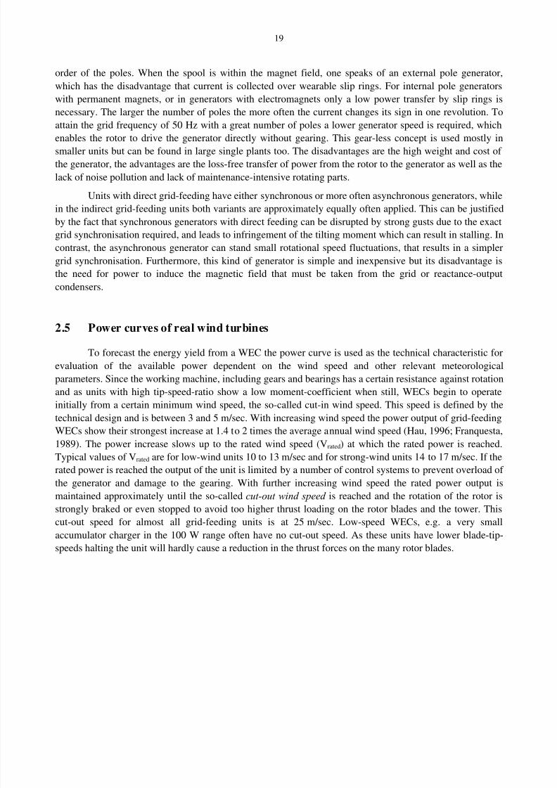
Figure 2.10: Power curve of a WEC with pitch control (Lagerwey 250 KW)
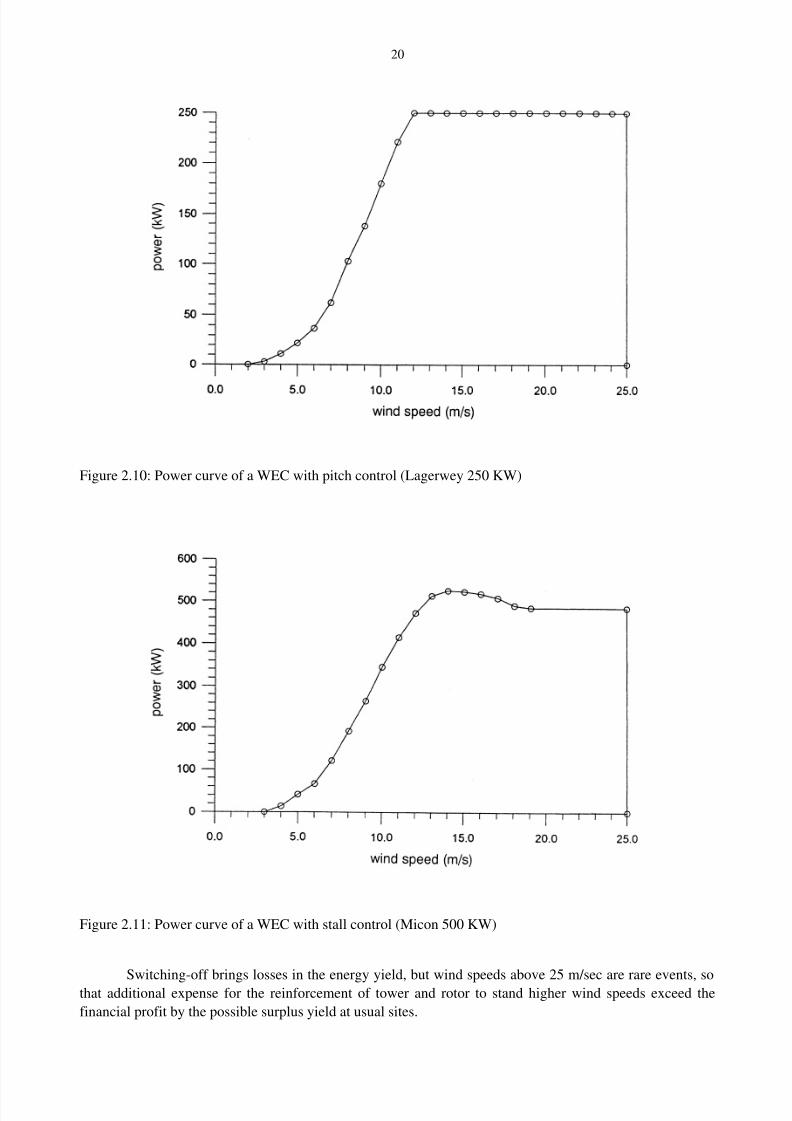
Figure 2.11: Power curve of a WEC with stall control (Micon 500 KW)
Switching-off brings losses in the energy yield, but wind speeds above 25 m/sec are rare events, sothat additional expense for the reinforcement of tower and rotor to stand higher wind speeds exceed the
financial profit by the possible surplus yield at usual sites.
8/2/2019 Dobesch Rpt
http://slidepdf.com/reader/full/dobesch-rpt 27/123
21
2.6 Control systems and yaw drives of WECs
For the necessary limitation of power output from WECs beyond their rated performance there are
different control systems available but the choice of pitch or stall control is still a matter of discussion. In
small units the tower head is often installed eccentrically before the mast axis and held in the wind in the
partial-load range by means of a spring. Above the rated wind speed, the wind thrust presses the rotor out of the wind and reduces the effective surface area for power production. Turning from the perpendicular into
the so-called „helicopter-position” allows power reduction. Bigger units with direct feeding into the grid
often use the effect of stalling at the rotor blade. Because the rotor is strictly bound to the grid frequency
with constant rotation speed for increasing wind speed the angle of attack of the rotor blade profile in
upwind direction (see paragraph 2.3.2) is increased. If an angle of above 15-20 degrees is reached flow
separation occurs from the profile upper side together with strong eddy development. From this the
resistance is increased strongly and the power is reduced. The great advantage of this control system is that a
simple connection of the rotor blade on the hub is possible. For very big units and units with indirect feeding
into the grid usually a blade-angle adjustment (pitch) is applied for power limitation. Through the variation
of the angle of attack and the resulting tip-speed ratio the power and rotational speed is regulated. The
disadvantage of costlier technical regulation should be compared with the advantages of increased efficiency
in the partial-load range and no additional cut-out mechanism during storms. With stall-regulated units the
cut-out during storms is by means of aerodynamic brakes like adjustable blade tips or movable spoilers.
Almost all WECs with stall - and pitch control, have a secondary mechanical brake for emergencies
The yaw drive of a WEC with horizontal axis either takes place passively or actively. A passive yaw
drive is effected by the attachment of the rotor in the lee of the tower, but for generators with high tip-speed-
ratio and low area coverage of the rotor-circle surface this principle only works for a moving rotor. In the
case of stall either the nacelle side wall must be used or an additional surface must be installed in the lee of
the tower. With the positioning of the rotor on the windward side of the tower a passive yaw drive is possible
if a wind vane with a sufficiently long lever arm is placed in the lee. This possibility is only used at smaller
units, because the required material expenditure is too high for larger WECs. Active yaw drive was achievedpreviously by a slower running wind wheel with high torque attached to the side of the nacelle, that started to
spin when crosswind components occurred and transferred this movement by a worm gear to the mounting
ring of the tower connection. Nowadays the application of an electric support motor is commonly used, that
is triggered by a small wind vane appropriately mounted at the nacelle. The disadvantage of this system lies
in the wind vane, which can for example be disturbed in its function by icing (Hau, 1996, Franquesta, 1989).
2.7 Technical availability and life span of WECs
Under the technical availability of a WEC one compares the ratio of the actual output from theconverter to the extractable annual energy yield. This ratio reached in early installations of the Californian
wind farms was often only 0.6 but nowadays the value reaches up to 0.98. The causes for the two percent
loss in “mass-produced” WECs are manifold. To gain a better overview they are divided into internal and
external causes. Whereas the internal faults causes (for example faulty management software or faulty
component material) are specific for certain WEC-types, the external ones show strong site dependence.
From the Institute for Solar Energy Supply Technology (ISET) at the University of Kassel (Germany) the
following table was compiled.

8/2/2019 Dobesch Rpt
http://slidepdf.com/reader/full/dobesch-rpt 28/123
22
Table 2.5: Frequency (%) of external damage causes for different site categories (Energiewerkstatt, 1995)
Region Grid-disconnection Lightening Icing Storm
Coastal area (43%) 69 22 16 24
North-German Plains (36%) 8 21 19 29
Sub-alpine mountains (21%) 23 57 65 47
Of the four main causes for external faults as grid-disconnection, lightning, icing and storm, in the
coastal area of Northern Germany up to two thirds of grid-disconnection was responsible and icing rarely
occurred, whereas in the German sub-alpine mountains the main causes were lightning and icing (c.f.
paragraph 3.4. and 3.5).
The life span can be dramatically influenced by lightning. Therefore at present the following
lightening protection concepts are observed: The use of a non-conducting rotor blade material without an
additional lightning protection, application of an aluminium cap at the blade top and an aluminium band
along the blade edge or application of a steel cap at the blade tips and lightning-conducting copper tissues atthe other blade surfaces.
The first concept is technically the simplest and cheapest but has the disadvantage that by surface
contamination and condensation of water conductivity on the blade surface can be established and then no
lightning protection exists. The second concept provides sufficient protection for the part most at risk, the
blade tip, however the rest of the blade remains unprotected. The third concept provides the highest
protection for the whole blade but is the most expensive (Dwenger, 1995).
In order to reach a life span of 20 years or more a high standard of durability of the components is
required. While for standard parts like the gearing or generators the longevity could readily be proven from
reliable information of numerous tests but for the rotor blades this is rare. To reach higher durability, instead
of glass fibre a carbon-fibre reinforced plastic can be chosen which requires enhanced lightning protection. It
is presently assumed, on the basis of the economic insecurity, that the maximum life span for a unit is 15
years.
8/2/2019 Dobesch Rpt
http://slidepdf.com/reader/full/dobesch-rpt 29/123
23
3 METEOROLOGICAL PARAMETERS IMPORTANT FOR THESITING PROCEDURE AND THE LIFE SPAN OF WECS
The main factors influencing the wind field in the boundary layer of the atmosphere are the large-
scale gradients of pressure and temperature, the earth rotation, the roughness of the earth surface, the daily
course of stability, the depth of the boundary layer, horizontal advection (of heat and momentum), certainmeteorological conditions such as clouds and rainfall and topographic properties (influencing the local and
meso-scale circulation as mountain wind systems and sea breezes).
Whereas large-scale differences in wind climatologies allow identification of regions with propitious
wind resources, the small scale phenomenon of the atmosphere in space and time e.g. turbulence and rare
events such as hail, icing and lightning, are important for the construction and operation of wind turbines and
for the selection of the optimal site for a given technology. This requires exact knowledge of the local spatial
variation of the wind vector in the lowest 100 meters of the atmospheric boundary layer.
The basis of yield estimate from wind energy for certain sites is comprised of topics from
meteorology, topography, technical construction of WECs, economy, local infrastructure, people’s
perception, natural and landscape protection, land use, noise emission, safety areas for airports and military
facilities and others. Additional measurements of hourly or 10-min averages of wind speed and wind
direction must be available as well as the 2-dimensional probability distribution of these properties and the
gustiness and/or standard deviation (cf. paragraph 7.1.2). Additionally some climatological fingerprints must
be known as the annual course of wind speed, its absolute maximum, the long-term average of air density,
the 2-dimensional frequency distribution of air temperature and air humidity, the number of hours with
heavy rain or hail and the number of days with storms and/or lightning strikes.
Concentrating here uniquely on the meteorological parameters which can be subdivided into three
groups: The first group determines the amount of the momentary power output and comprises air density and
wind speed, the second group determines the energy yield during the entire time of operation and comprises
the frequency-distribution of the wind speed, seasonal variability, the number of the days with icing of therotor blades, and finally the third group with an important parameters for the live span of the WEC, is
lightning strikes, icing, hail and maximum wind gusts. Sound emission and shadow casting are treated in
chapter 8 because these strongly influence the choice of the site due to certain legislative restrictions rather
than meteorological conditions. Problems of corrosion and high turbulence are more an issue in tropical
areas and are addressed extensively in WMO/TD-No.826 ("Meteorological Aspects and Recommendations
for Assessing and Using the Wind as an Energy Source in the Tropics").
3.1 The air density
3.1.1 Definition
The air density is defined as the mass of an air-package standardised with unit volume. The air
density is a function of space and time, where especially the vertical height dependence is essential for
questions concerning wind energy. The air, showing a variable density, is considered as a compressible
medium. For dry air at sea level with an atmospheric pressure of p = 1013.25 hPa and a temperature of
288 K the pressure amounts to
(3.1)2
0 2251 mkg / .=ρ
8/2/2019 Dobesch Rpt
http://slidepdf.com/reader/full/dobesch-rpt 30/123
24
3.1.2 The height dependency of the air density
Because there are only very slight differences in air density during a season at a certain height, for
reasons of simplicity the height dependency is taken into account only for the hydrostatic fundamental
equation
(3.2) dp z gdz = −ρ ( )
For air with good approximation the equation of state for ideal gases is valid
(3.3) p RT = ρ
with T the absolute temperature in Kelvin (K) and R the gas constant, which for air amounts to
(3.4) K s
m
R ⋅= 2
2
287
To calculate the function p(z) and ρ (z) the temperature gradient T(z) must be known. By appropriate
assumptions about T(z) corresponding models for the description of the atmosphere can be derived. Linear
temperature gradients (isentropic and polytropic atmosphere) play the most important role. Isentropy means
that there is no heat exchange with the surroundings (adiabatic) and no friction-losses (reversible) if a
movement of the air mass to other heights occurs due to external disturbances. For the adiabatic reversible
change in state for ideal gases it is valid:
(3.5) .'0
'
0konst p
p
== κ
κ
ρ
ρ
The parameter κ ’ is called the isentropic exponent and is for air κ ’ = 1.4. From Eq.(3.5) it follows after the
integration of Eq.(3.2) the density course in the isentropic atmosphere ( H o = height of the homogenous
atmosphere) is:
(3.6) 1'
1
0
0 )'
1'1()( −−
−= κ
κ
κ ρ ρ
H
z z
For the polytropic atmosphere the general (empirical) formulation is:
(3.7) .'
0
'
0
konst p
pn
n
==ρ
ρ
with n’ the polytropic exponent. For the polytropic atmosphere the same density course as for the isentropic
atmosphere is valid where κ ’ is replaced by n’ . For n’ = 1,235 and H 0 = 8434 meters it follows from
Eq.(3.6)
(3.8)25532.4
0 0000226.01()( z) z −= ρ ρ
Another approach is the following frequently used formula:
8/2/2019 Dobesch Rpt
http://slidepdf.com/reader/full/dobesch-rpt 31/123
25
(3.9)294 100267.4101743.12255.1)( z z z −− ⋅+⋅−=ρ
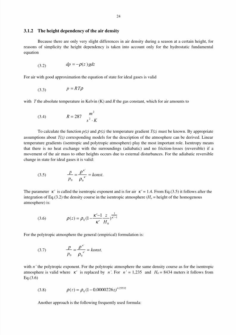
An example for ρ (z) and ρ (z)/ ρ 0 is given in Table 3.1 for the first 3000 meters of the standard atmosphere
Table 3.1: Density and relative density of air dependent on height
Height (m) ρ (kg/m3) ρ / ρ 0 Height (m) ρ (kg/m
3) ρ / ρ 0
0 1.225 1.000 1200 1.090 0.890100 1.213 0.990 1400 1.069 0.872200 1.202 0.981 1600 1.048 0.855300 1.190 0.972 1800 1.027 0.838400 1.179 0.962 2000 1.006 0.822500 1.167 0.953 2200 0.986 0.805600 1.156 0.944 2400 0.967 0.789700 1.145 0.935 2600 0.947 0.773800 1.134 0.925 2800 0.928 0.758
900 1.123 0.916 3000 0.909 0.7421000 1.112 0.907
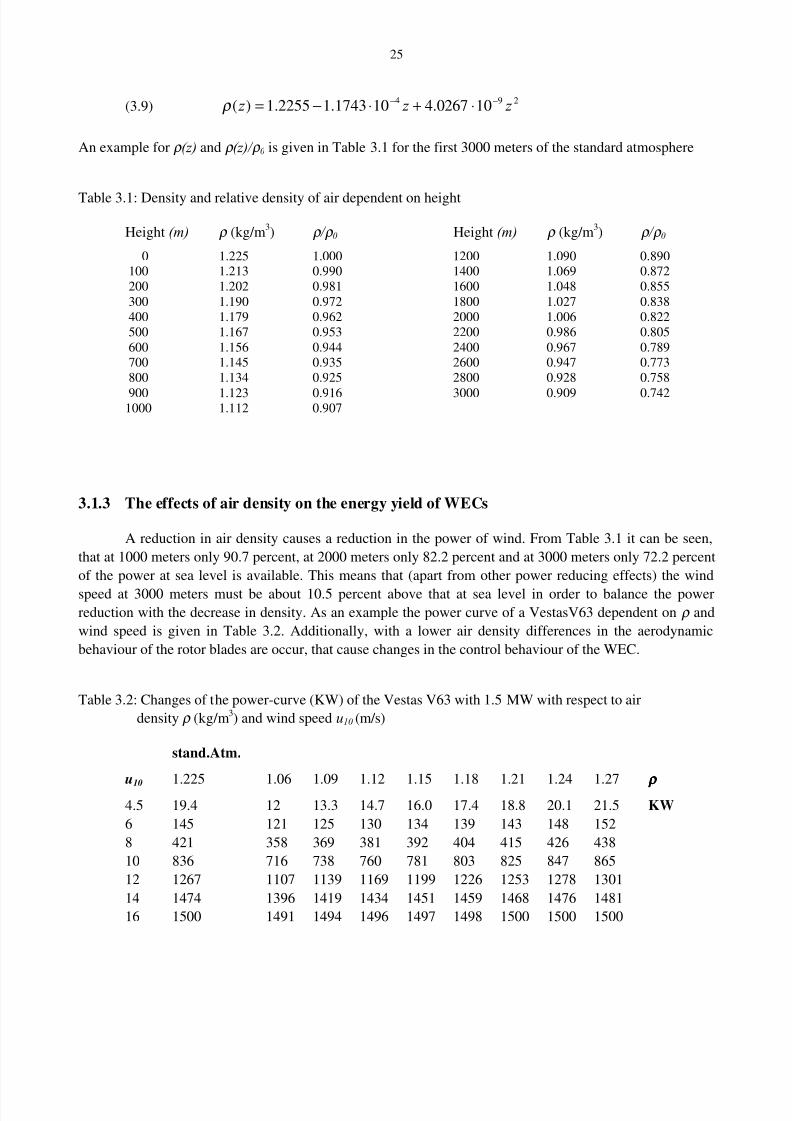
3.1.3 The effects of air density on the energy yield of WECs
A reduction in air density causes a reduction in the power of wind. From Table 3.1 it can be seen,
that at 1000 meters only 90.7 percent, at 2000 meters only 82.2 percent and at 3000 meters only 72.2 percent
of the power at sea level is available. This means that (apart from other power reducing effects) the wind
speed at 3000 meters must be about 10.5 percent above that at sea level in order to balance the powerreduction with the decrease in density. As an example the power curve of a VestasV63 dependent on ρ and
wind speed is given in Table 3.2. Additionally, with a lower air density differences in the aerodynamic
behaviour of the rotor blades are occur, that cause changes in the control behaviour of the WEC.
Table 3.2: Changes of the power-curve (KW) of the Vestas V63 with 1.5 MW with respect to air
density ρ (kg/m3) and wind speed u10 (m/s)
stand.Atm.
u10 1.225 1.06 1.09 1.12 1.15 1.18 1.21 1.24 1.27 ρ ρρ ρ 4.5 19.4 12 13.3 14.7 16.0 17.4 18.8 20.1 21.5 KW
6 145 121 125 130 134 139 143 148 152
8 421 358 369 381 392 404 415 426 438
10 836 716 738 760 781 803 825 847 865
12 1267 1107 1139 1169 1199 1226 1253 1278 1301
14 1474 1396 1419 1434 1451 1459 1468 1476 1481
16 1500 1491 1494 1496 1497 1498 1500 1500 1500

8/2/2019 Dobesch Rpt
http://slidepdf.com/reader/full/dobesch-rpt 32/123
26
3.2 The spatial distribution of the wind vector
Much information can be found in the appropriate literature about global and regional wind
meteorologies and climatologies (e.g. WMO No.175, Mortensen et al., 1993; Dobesch et al., 1997). But
because this is an important aspect in assessing wind power potential, the main features of the global and
local wind system will be outlined here.
Usually one distinguishes when investigating wind climates, the large- and small-scale flows.
Whereas the large-scale flows are governed by the global distribution of the air pressure systems
(Großwetterlagen), the small-scale flows are additionally influenced by the atmospheric properties due to the
change of day and night and to the local orographic conditions. As a consequence quite different approaches
for describing the resulting wind fields have to be followed.
3.2.1 Large-scale wind flows
The driving force for global circulation is the sun giving an average flux of solar energy at the
earth’s surface equal to 350 W/m-2 (Goody et al., 1989). Of this energy approximately 31 percent is scattered
back into space, 43 percent is absorbed at the earth’s surface and 26 percent is absorbed by the atmosphere.
Considering the back scattered portion, the albedo (ratio of outward to incoming flux of solar radiation)
allows an average of 225 W/m-2
available for heating, directly and indirectly the earth and its atmosphere.
From the curvature of the earth’s surface and the seasonal variation of the position of the axis of the earth to
the sun, the irradiation is spatially and temporally very different in its distribution across the earth’s surface.
In consideration of these differences in the irradiance as well as the regional differences in the albedo and the
black-body radiation, that is proportional to the fourth power of the temperature of the radiating surface, the
spatial distribution of the annual total radiation balance of the earth’s surface is established causing large-
scale temperature gradients resulting in the global circulation system.
It is now shown briefly how the global circulation results from this temperature pattern starting withthe equation of motion. In an inertia system the forces of pressure, gravity and friction have to be considered.
For the pressure force acting on a mass m can be written (Holton, 1992):
(3.10) pm
K →→
∇−=ρ
1
The friction force results from molecular forces of two flow layers moving with different velocities and is
proportional to the curvature of the velocity profile in the co-ordinate axes:
(3.11) ∑=
→
j j
iir
x
v
m
K 2
2
∂
∂ ν
,
Because the rotating earth is used as the reference system the centrifugal and Coriolis forces have to be
considered. The centrifugal force acts vertically to the axis of rotation and is proportional to the square of the
angular velocity of the earth (Holton, 1992):
(3.12)
→→
−= r m
K z 2
ω

8/2/2019 Dobesch Rpt
http://slidepdf.com/reader/full/dobesch-rpt 33/123
27
The angular velocity ω results from the rotation of the earth around her own axis in 23h 56min 4s
(= 1 siderial day), its value amounts therefore to ω = 7.3x10⁻⁵
rad/s. Because the centrifugal force depends
additionally on the distance to the axis of rotation its amount is greatest at the equator and at the poles
equally zero.
The Coriolis force can be written with the vector of the earth’s rotation Ω
→
(ω = Ω
→
) as
(3.13) ],,[, wvuuvm
K c ×Ω−=→
→
2
Now the momentum equations of the atmosphere can be summarised in vector notation
(3.14) ],,[, g g m
K g pv
dt
vd r −=++∇−×Ω−=→
→→→→→
→
001
2ρ
In large-scale flows, the friction can be neglected so that for horizontal stationary flows the
following approximations yields:
(3.15) x
pv
dt
du
∂
∂
ρ ϕ ω
120 −== sin
(3.16) y
pu
dt
dv
∂
∂
ρ ϕ ω
120 −−== sin
These equations are called geostrophic approximations. By means of these relations it is possible to define a
wind vector, the so-called geostrophic wind :
(3.17) p f
k vc
g
→→→
∇×≡ρ
1
→
k being the unit vector in the vertical and f c the Coriolis parameter (=2ω sinϕ = 1.45.10-4
s-1
sinϕ). The
geostrophic wind after Eq.(3.19) however is only valid in uncurved flow. To account for an existing
curvature of the isobars the amount of v g has to be modified by the given centrifugal force whereas thedirection is maintained. Therefore with the curvature 1/r it can be written for cyclonal curvature
(3.18)r
vv f
n
pc
21+=
∂
∂
ρ
and for anticyclonal curvature
(3.19)r
vv f
n
pc
21−=
∂
∂
ρ

8/2/2019 Dobesch Rpt
http://slidepdf.com/reader/full/dobesch-rpt 34/123
28
The wind resulting from this pressure distribution is usually called gradient-wind which is smaller in
cyclonal flow and greater for anticyclonal curvature than the geostrophic wind with the same pressure
gradient.
3.2.2 Small-scale wind systems
Small-scale wind systems usually result from pressure differences caused by the different conditions
of the atmosphere during day and night. These pressure differences have their origin in the different speeds
and amount of the transformation of radiation energy into heat (and vice versa), which emerges from the
properties and condition of the earth’s surface. A typical example for this is the land-sea breeze or the
mountain valley circulation (see paragraph 5.2.2). Mathematically a circulation can be formulated as
(3.20)→→
∫ = sd v Z .
with→
v the velocity vector and→
sd the path element along the closed curve. By expressing the acceleration
dt vd / →
in the pressure gradient form, it follows
(3.21) ∫ = dpdt
dZ α
with α the specific volume, the inverse of the density. A more descriptive form is obtained, if the specific
volume is substituted by the equation of state for ideal gases:
(3.22) ∫ = pd T Rdt
dZ L ln
with R L the gas constant of the air and T the absolute temperature. An estimation of the circulation
acceleration when investigating of sea-breezes in coastal regions or large lakes for example can be made by
the simple formula
(3.23) p R
T T
dt
dZ
L
W L ∆⋅−
= ln)(
with T L and T W the temperature of the land and water surface and ∆ p the pressure difference. In general a
sea-breeze circulation can reach horizontally up to 80 km with a vertical extend of approximately one
kilometre with wind speeds of 5 to 8 m/s. In Djakarta (Indonesia) close to the equator sea-breezes were
observed with a speed of 10 m/s and a vertical extend of 4 km. In contrast to sea breeze the land wind
circulation at night is much less developed and reaches only an extent from 300 – 500 meters (Haeckl, 1990,
WMO 175).
In more complex mountain regions orographical wind systems develop, being generally weaker than
the land- and sea-breeze systems but considerably stronger where additionally channelling effects occur. A
typical example of such a superimposition represents the wind system of Lake Garda, Italy. Another
possibility for high and continuous wind speeds in valleys occur if the main wind direction lies parallel to the
valley axis. A further discussion about orographic induced flows is given in chapter 5.2.
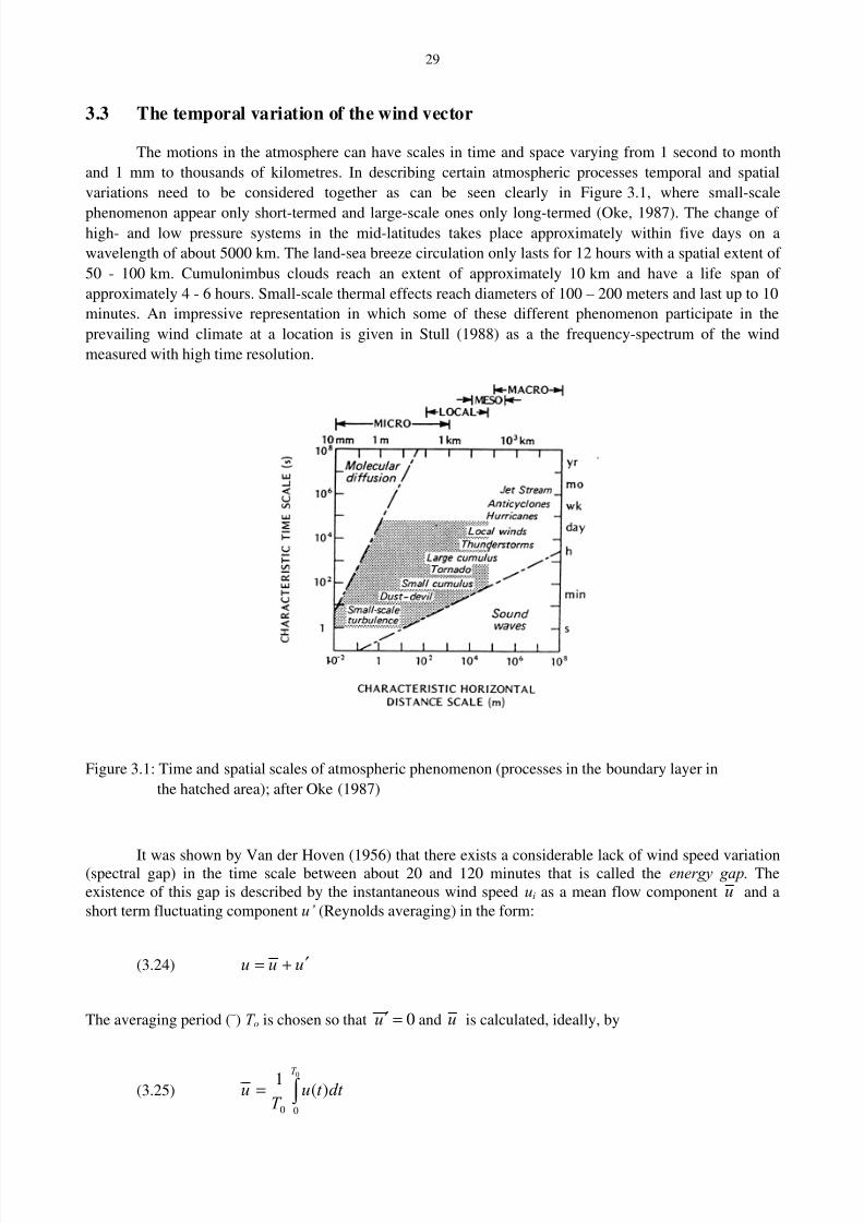
8/2/2019 Dobesch Rpt
http://slidepdf.com/reader/full/dobesch-rpt 35/123
29
3.3 The temporal variation of the wind vector
The motions in the atmosphere can have scales in time and space varying from 1 second to month
and 1 mm to thousands of kilometres. In describing certain atmospheric processes temporal and spatial
variations need to be considered together as can be seen clearly in Figure 3.1, where small-scale
phenomenon appear only short-termed and large-scale ones only long-termed (Oke, 1987). The change of high- and low pressure systems in the mid-latitudes takes place approximately within five days on a
wavelength of about 5000 km. The land-sea breeze circulation only lasts for 12 hours with a spatial extent of
50 - 100 km. Cumulonimbus clouds reach an extent of approximately 10 km and have a life span of
approximately 4 - 6 hours. Small-scale thermal effects reach diameters of 100 – 200 meters and last up to 10
minutes. An impressive representation in which some of these different phenomenon participate in the
prevailing wind climate at a location is given in Stull (1988) as a the frequency-spectrum of the wind
measured with high time resolution.
Figure 3.1: Time and spatial scales of atmospheric phenomenon (processes in the boundary layer in
the hatched area); after Oke (1987)
It was shown by Van der Hoven (1956) that there exists a considerable lack of wind speed variation(spectral gap) in the time scale between about 20 and 120 minutes that is called the energy gap. Theexistence of this gap is described by the instantaneous wind speed ui as a mean flow component u and a
short term fluctuating component u’ (Reynolds averaging) in the form:
(3.24) uuu ′+=
The averaging period (–) T o is chosen so that 0=′u and u is calculated, ideally, by
(3.25) ∫ =0
00
)(1 T
dt t uT
u
8/2/2019 Dobesch Rpt
http://slidepdf.com/reader/full/dobesch-rpt 36/123
30
or simply from N numbers of measurement by
(3.26) ∑=
= N
i
iu N
u1
1
In order to simplify the calculation this average value is usually assumed as ergodic that means the spatial,
temporal and the ensemble average are identical.
To characterise the short-term fluctuations within the averaging period the variance and the standard
deviation of the wind speed is taken as
(3.27)2
1
2 1)( uu
N
N
i
iu −= ∑=
σ
and
(3.28)212 / )(uu
′≡σ
Furthermore, in horizontal homogenous terrain the turbulence intensity can be written as
(3.29) u I u / σ =
The actual turbulence depends on the complexity of the terrain, the roughness of the land surface
including single-standing obstacles on the windward side of the site, the existing vertical wind profile and
the density stratification of the atmosphere. Typical values of the turbulence intensity lie between 0.08 for a
smooth, even surface with stable density stratification and 0.5 for strongly inhomogeneous terrain with
unstable density stratification. Because increasingly fluctuating aerodynamic forces originate with increasing
turbulence intensity at the rotor blade, the knowledge of this parameter is for a certain site very important for
WEC installation (Molly, 1990; Wieringa, 1973). The turbulence intensity can be simplified for homogenous
surface roughness z o and neutral conditions to Ι ≈ 1/ln(z/z o ).
Though different investigations it has been shown that the frequency spectrum of the turbulence
derived from a point measurement on a mast differs quintessentially from that at a point on the rotor blade:
In fact for the low-frequency turbulence range the assumption is valid that the eddy includes the entire rotor
radius, consequently in this region the spectra are approximately the same. In the medium-frequency range
the entire rotor is no longer involved and as a consequence the rotor blade enters the eddy only for a short
time. Because of this the medium-frequency range is shifted into the high-frequency range where at each
integral multiple of the rotor revolution a deflection occurs. This difference between the turbulence spectrum
of an anemometer and that of a point on the rotor blade is illustrated in Figure 3.2.
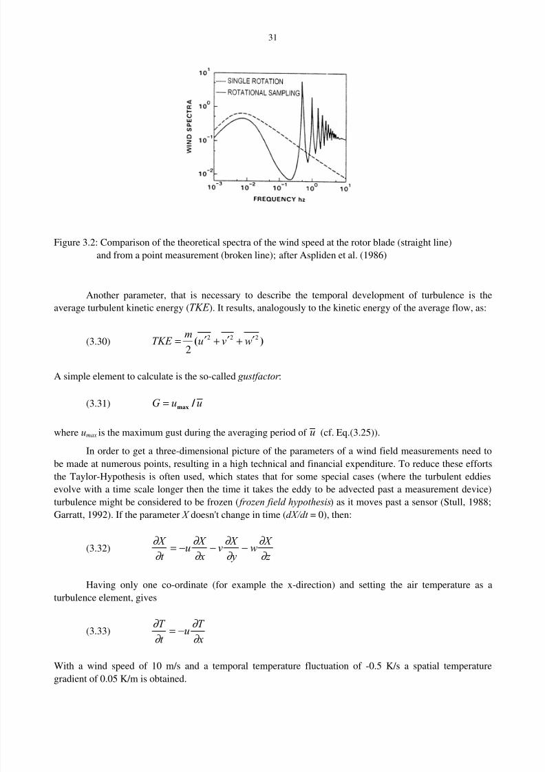
8/2/2019 Dobesch Rpt
http://slidepdf.com/reader/full/dobesch-rpt 37/123
31
Figure 3.2: Comparison of the theoretical spectra of the wind speed at the rotor blade (straight line)
and from a point measurement (broken line); after Aspliden et al. (1986)
Another parameter, that is necessary to describe the temporal development of turbulence is the
average turbulent kinetic energy (TKE ). It results, analogously to the kinetic energy of the average flow, as:
(3.30) )(222
2wvu
mTKE ′+′+′=
A simple element to calculate is the so-called gustfactor :
(3.31) uuG / max=
where umax is the maximum gust during the averaging period of u (cf. Eq.(3.25)).
In order to get a three-dimensional picture of the parameters of a wind field measurements need to
be made at numerous points, resulting in a high technical and financial expenditure. To reduce these efforts
the Taylor-Hypothesis is often used, which states that for some special cases (where the turbulent eddies
evolve with a time scale longer then the time it takes the eddy to be advected past a measurement device)
turbulence might be considered to be frozen ( frozen field hypothesis) as it moves past a sensor (Stull, 1988;
Garratt, 1992). If the parameter X doesn't change in time (dX/dt = 0), then:
(3.32) z X w
y X v
x X u
t X
∂ ∂
∂ ∂
∂ ∂
∂ ∂ −−−=
Having only one co-ordinate (for example the x-direction) and setting the air temperature as a
turbulence element, gives
(3.33) x
T u
t
T
∂
∂
∂
∂ −=
With a wind speed of 10 m/s and a temporal temperature fluctuation of -0.5 K/s a spatial temperature
gradient of 0.05 K/m is obtained.
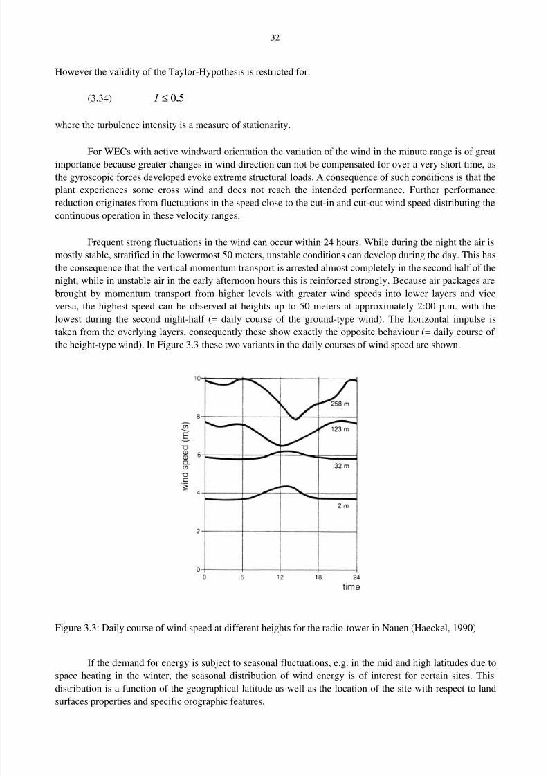
8/2/2019 Dobesch Rpt
http://slidepdf.com/reader/full/dobesch-rpt 38/123
32
However the validity of the Taylor-Hypothesis is restricted for:
(3.34) 50.≤ I
where the turbulence intensity is a measure of stationarity.
For WECs with active windward orientation the variation of the wind in the minute range is of great
importance because greater changes in wind direction can not be compensated for over a very short time, as
the gyroscopic forces developed evoke extreme structural loads. A consequence of such conditions is that the
plant experiences some cross wind and does not reach the intended performance. Further performance
reduction originates from fluctuations in the speed close to the cut-in and cut-out wind speed distributing the
continuous operation in these velocity ranges.
Frequent strong fluctuations in the wind can occur within 24 hours. While during the night the air is
mostly stable, stratified in the lowermost 50 meters, unstable conditions can develop during the day. This has
the consequence that the vertical momentum transport is arrested almost completely in the second half of thenight, while in unstable air in the early afternoon hours this is reinforced strongly. Because air packages are
brought by momentum transport from higher levels with greater wind speeds into lower layers and vice
versa, the highest speed can be observed at heights up to 50 meters at approximately 2:00 p.m. with the
lowest during the second night-half (= daily course of the ground-type wind). The horizontal impulse is
taken from the overlying layers, consequently these show exactly the opposite behaviour (= daily course of
the height-type wind). In Figure 3.3 these two variants in the daily courses of wind speed are shown.
Figure 3.3: Daily course of wind speed at different heights for the radio-tower in Nauen (Haeckel, 1990)
If the demand for energy is subject to seasonal fluctuations, e.g. in the mid and high latitudes due to
space heating in the winter, the seasonal distribution of wind energy is of interest for certain sites. Thisdistribution is a function of the geographical latitude as well as the location of the site with respect to land
surfaces properties and specific orographic features.
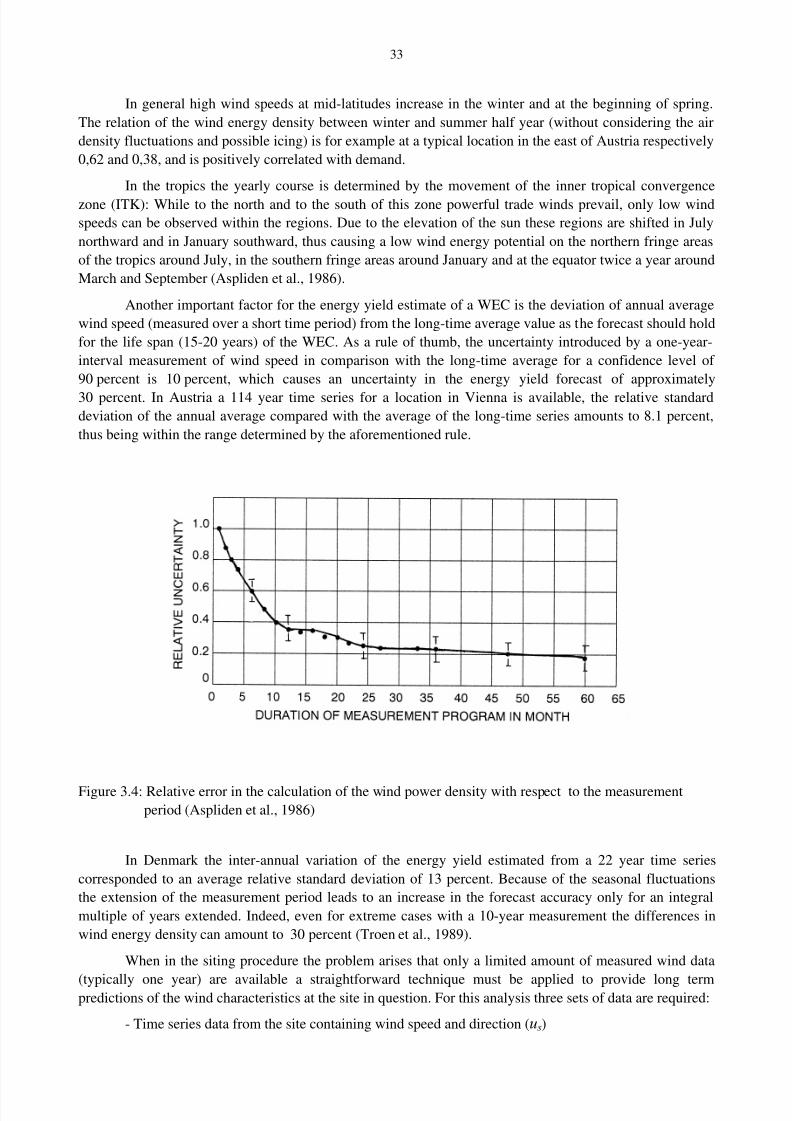
8/2/2019 Dobesch Rpt
http://slidepdf.com/reader/full/dobesch-rpt 39/123
33
In general high wind speeds at mid-latitudes increase in the winter and at the beginning of spring.
The relation of the wind energy density between winter and summer half year (without considering the air
density fluctuations and possible icing) is for example at a typical location in the east of Austria respectively
0,62 and 0,38, and is positively correlated with demand.
In the tropics the yearly course is determined by the movement of the inner tropical convergence
zone (ITK): While to the north and to the south of this zone powerful trade winds prevail, only low wind
speeds can be observed within the regions. Due to the elevation of the sun these regions are shifted in July
northward and in January southward, thus causing a low wind energy potential on the northern fringe areas
of the tropics around July, in the southern fringe areas around January and at the equator twice a year around
March and September (Aspliden et al., 1986).
Another important factor for the energy yield estimate of a WEC is the deviation of annual average
wind speed (measured over a short time period) from the long-time average value as the forecast should hold
for the life span (15-20 years) of the WEC. As a rule of thumb, the uncertainty introduced by a one-year-
interval measurement of wind speed in comparison with the long-time average for a confidence level of
90 percent is 10 percent, which causes an uncertainty in the energy yield forecast of approximately
30 percent. In Austria a 114 year time series for a location in Vienna is available, the relative standarddeviation of the annual average compared with the average of the long-time series amounts to 8.1 percent,
thus being within the range determined by the aforementioned rule.
Figure 3.4: Relative error in the calculation of the wind power density with respect to the measurement
period (Aspliden et al., 1986)
In Denmark the inter-annual variation of the energy yield estimated from a 22 year time series
corresponded to an average relative standard deviation of 13 percent. Because of the seasonal fluctuations
the extension of the measurement period leads to an increase in the forecast accuracy only for an integral
multiple of years extended. Indeed, even for extreme cases with a 10-year measurement the differences in
wind energy density can amount to 30 percent (Troen et al., 1989).
When in the siting procedure the problem arises that only a limited amount of measured wind data
(typically one year) are available a straightforward technique must be applied to provide long termpredictions of the wind characteristics at the site in question. For this analysis three sets of data are required:
- Time series data from the site containing wind speed and direction (u s)
8/2/2019 Dobesch Rpt
http://slidepdf.com/reader/full/dobesch-rpt 40/123
34
- Time series data from a meteorological station concurrent with the site data containing wind
speed and direction (um)
- Historical data from the same meteorological station in the form of a time series or a frequency
distribution table for wind speed and direction.
The site and meteorological station data are analysed to determine the correlation between the twosets of data in each of a number of directional sectors on the base of hourly values. This correlation is thenused with the historical data to predict the wind climate that would have existed at the wind farm site duringthat historical period. The wind speeds are binned into directional sectors, and within each sector a linearbest fit is applied which relates the wind speed at the meteorological station to that at the site. i.e. for anarbitrary direction
(3.35) u s = c1 um + c2
The linear best fit can be made e.g. by standard least squares techniques or the York method (Press et
al.,1992). This York method fits a strait line through the N data points (u s1 , um1), …, (u sn , umn) so that the
sum of the squares of the distances of those points from the straight line is a minimum, where the distance ismeasured in the direction calculated by taking the relative errors of both data sets into account. Hence the
chi-squared merit function
(3.36)
is minimised which is the approach behind the York method.
A further improvement for the data from the site is that the frequency table, generated from the
correlation process, can also be corrected for veer. The basis of the veer correction is to bin the hourly data
from the meteorological station and site direction data into a square matrix (with the same dimensions as the
historical direction sectors). This matrix is then normalised and used to redistribute the frequency data
generated from the meteorological historical data to the final site frequency table.
3.4 The influence of precipitation events
3.4.1 Heavy rain
Slight or moderate rain does not influence the performance of a WEC. During heavy rain however
massive drop impacts occur at the rotor blades through which the flow around the profile is disturbed
considerably. From measurements power losses up to 30 percent could be found according to the intensity
of rain. The comparison of power curves with and without rain is illustrated in Figure 3.5. How far heavy
rain influences the yearly energy yield can be made evident from the two-dimensional frequency distribution
of precipitation and wind speed. However, it is to be expected that strong rain events will affect the operation
of the WEC during partial load, as this range delivers the greatest share of the energy yield.
∑= +
−−=
N
i sm
simi
c
uccucc
12
12
2
1221
2
σ σ χ
)(),(
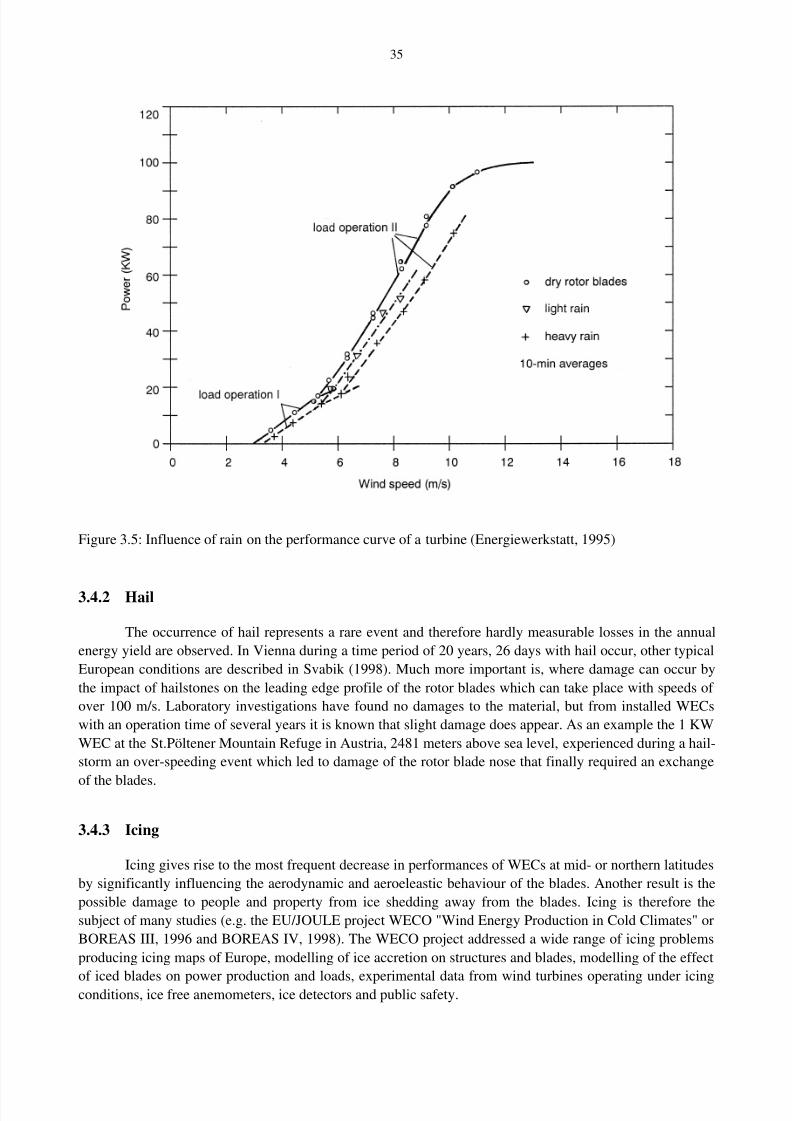
8/2/2019 Dobesch Rpt
http://slidepdf.com/reader/full/dobesch-rpt 41/123
35
Figure 3.5: Influence of rain on the performance curve of a turbine (Energiewerkstatt, 1995)
3.4.2 Hail
The occurrence of hail represents a rare event and therefore hardly measurable losses in the annual
energy yield are observed. In Vienna during a time period of 20 years, 26 days with hail occur, other typical
European conditions are described in Svabik (1998). Much more important is, where damage can occur by
the impact of hailstones on the leading edge profile of the rotor blades which can take place with speeds of
over 100 m/s. Laboratory investigations have found no damages to the material, but from installed WECs
with an operation time of several years it is known that slight damage does appear. As an example the 1 KW
WEC at the St.Pöltener Mountain Refuge in Austria, 2481 meters above sea level, experienced during a hail-
storm an over-speeding event which led to damage of the rotor blade nose that finally required an exchange
of the blades.
3.4.3 Icing
Icing gives rise to the most frequent decrease in performances of WECs at mid- or northern latitudes
by significantly influencing the aerodynamic and aeroeleastic behaviour of the blades. Another result is the
possible damage to people and property from ice shedding away from the blades. Icing is therefore the
subject of many studies (e.g. the EU/JOULE project WECO "Wind Energy Production in Cold Climates" or
BOREAS III, 1996 and BOREAS IV, 1998). The WECO project addressed a wide range of icing problems
producing icing maps of Europe, modelling of ice accretion on structures and blades, modelling of the effect
of iced blades on power production and loads, experimental data from wind turbines operating under icingconditions, ice free anemometers, ice detectors and public safety.

8/2/2019 Dobesch Rpt
http://slidepdf.com/reader/full/dobesch-rpt 42/123
36
Two prerequisites are necessary for the appearance of icing on the rotor blades: Firstly the surface
temperature must lie beneath 0°C and secondly supercooled water droplets, i.e. liquid water at temperatures
below 0°C must occure. It is valid that the smaller the drop diameter is the more strongly will be the
supercooling, reaching -40°C at its lowest limit.
The icing process results from either
• Impingement of supercooled water droplets or wet snow on the blade surface by which the
inner structure of the droplet is disturbed and the freezing point raised to 0°C. Sudden
freezing is the consequence. Ice accretion is therefore found particularly on those parts of the
WEC, that are exposed to a frontal impact of the water droplets.
• Sublimation on the blades
• Energy balance favouring ice formation
3.4.3.1 Types of icing
In general one distinguishes 4 types of icing: Clear-ice (glaze, blue ice), rough-ice, hoarfrost and
rime ice.
Clear-ice forms a transparent icecap with a glassy surface that originates by the accretion of freezing
rain with temperatures between 0°C and -4°C. The icecap adapts itself to the form of the enclosed object and
can hardly be removed from it. The very smooth surface results from the fact that the droplets during the
impact freeze not immediately completely because of the released heat (335 kJ/kg water) during the freezing
process and so the water is evenly distributed across the surface by the flow.
Rough ice is produced if the rain contains crystals of ice, snow or sleet. The icecap looses its smooth
transparent surface and becomes granulated and appearing whitish-opaque. This ice accretion occurs with air
temperatures from -4°C to -9°C and is among the most frequent forms of icing. From the inherent snow andsleet a strong influence on the aerodynamics of the rotor blades can occur.
Hoarfrost appears, if fine water droplets with temperatures of less than -10°C impact the WEC and
instantly freeze completely. As the drops can no longer flow together the accretion grows against the airflow
around edges in the form of humps. From the accreted snow crystals a rough surface develops appearing
brittle and milky, also containing air bubbles. The profile-form of the blades is changed massively such the
power output is greatly reduced. Furthermore, as fragments easy separate from the rotor blades, these can be
hurled away up to a distance up to three rotor diameters during operation.
Rime ice is the most common type of in cloud icing and forms on the upwind side of structures. The
most severe occurrence is found on widely exposed mountains and hills. Different types of rime may be
distinguished in accordance with their density, hardness and appearance:
Hard rime is granular and adheres firmly on surfaces; its density ranges between 100 and 600 kg/m3;
Soft rime is a fragile snow-like formation with a density less than 100 kg/m3;
Metamorphosed rime is rime ice altered due to sublimation.
Rime icing has hardly any effects on the operation of WECs (Eichenberger, 1990).
3.4.3.2 The physical background of icing
The physical mechanisms associated with ice accretion are numerous and complex and can bedivided roughly into 3 categories:
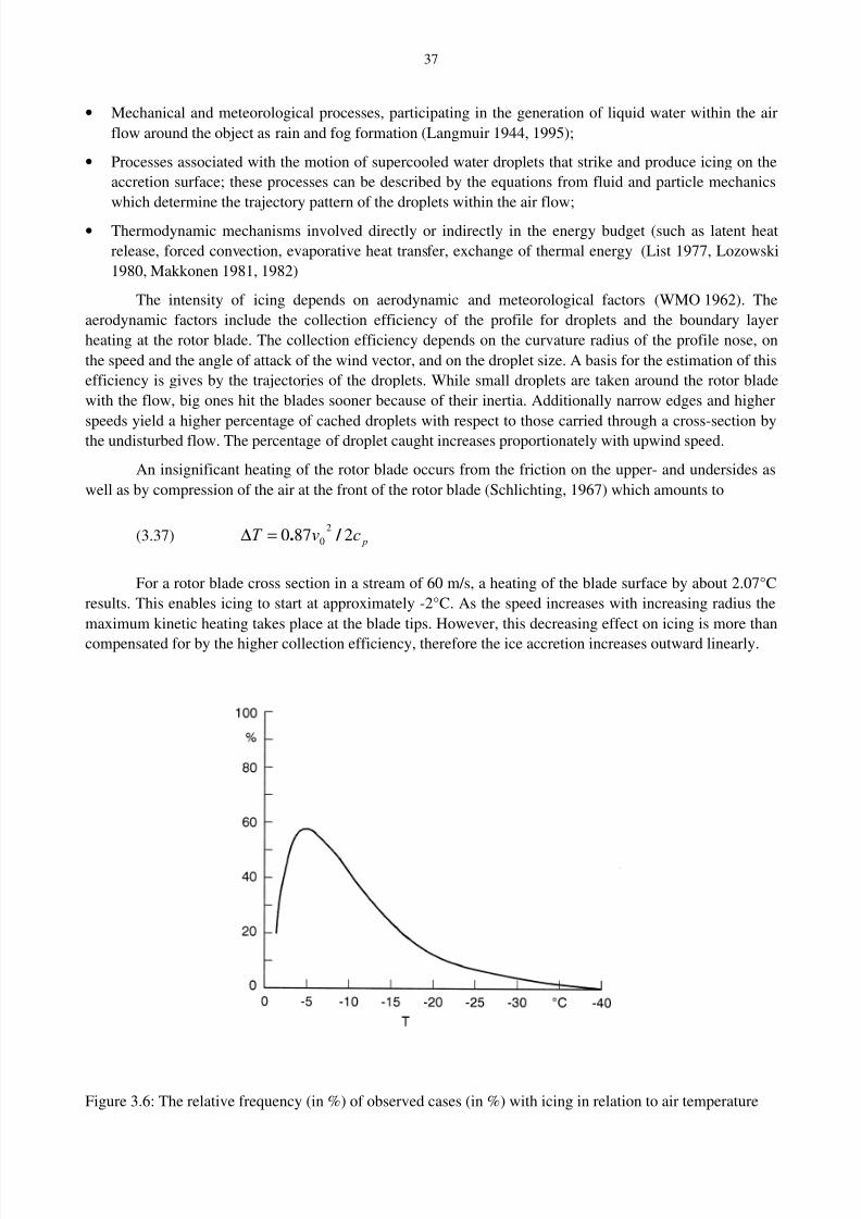
8/2/2019 Dobesch Rpt
http://slidepdf.com/reader/full/dobesch-rpt 43/123
37
• Mechanical and meteorological processes, participating in the generation of liquid water within the air
flow around the object as rain and fog formation (Langmuir 1944, 1995);
• Processes associated with the motion of supercooled water droplets that strike and produce icing on the
accretion surface; these processes can be described by the equations from fluid and particle mechanics
which determine the trajectory pattern of the droplets within the air flow;
• Thermodynamic mechanisms involved directly or indirectly in the energy budget (such as latent heat
release, forced convection, evaporative heat transfer, exchange of thermal energy (List 1977, Lozowski
1980, Makkonen 1981, 1982)
The intensity of icing depends on aerodynamic and meteorological factors (WMO 1962). The
aerodynamic factors include the collection efficiency of the profile for droplets and the boundary layer
heating at the rotor blade. The collection efficiency depends on the curvature radius of the profile nose, on
the speed and the angle of attack of the wind vector, and on the droplet size. A basis for the estimation of this
efficiency is gives by the trajectories of the droplets. While small droplets are taken around the rotor blade
with the flow, big ones hit the blades sooner because of their inertia. Additionally narrow edges and higher
speeds yield a higher percentage of cached droplets with respect to those carried through a cross-section bythe undisturbed flow. The percentage of droplet caught increases proportionately with upwind speed.
An insignificant heating of the rotor blade occurs from the friction on the upper- and undersides as
well as by compression of the air at the front of the rotor blade (Schlichting, 1967) which amounts to
(3.37) pcvT 28702
0 / .=∆
For a rotor blade cross section in a stream of 60 m/s, a heating of the blade surface by about 2.07°C
results. This enables icing to start at approximately -2°C. As the speed increases with increasing radius the
maximum kinetic heating takes place at the blade tips. However, this decreasing effect on icing is more than
compensated for by the higher collection efficiency, therefore the ice accretion increases outward linearly.
Figure 3.6: The relative frequency (in %) of observed cases (in %) with icing in relation to air temperature
8/2/2019 Dobesch Rpt
http://slidepdf.com/reader/full/dobesch-rpt 44/123
38
As already mentioned, a prerequisite for icing is supercooled water droplets. Their number depends
beside other factors on the air temperature. Between 0°C and -12°C the water particles are in the majority, in
the range between -13°C to -20°C the number of ice and water particles is approximately equal, between -
21°C and -40°C the ice particles prevail and below -40°C only ice particles exist. Because the ice particles in
the air create no icing, the icing probability decreases strongly below -12°C. In aviation three quarters of the
icing cases are observed above -15°C. The greatest icing probability lies between -4°C and -8°C. Theamount of icing depends therefore strongly on the temperature. Because the freezing process of the liquid
droplets is started by freezing nuclei and is dependent on their size, larger drops with a diameter of 1 mm are
supercooled only down to -15°C, while smaller droplets with 10-20 µm diameter can reach -30°C. This
means that essentially greater ice accretion is possible with temperatures just below 0°C, as the largest drops
exist in this range. The relative air humidity plays a role in this respect too, as the ice particles grow during
fog at the expense of water particles: This reduces the relative humidity to a value that corresponds to
saturation above ice. The relative humidity of air is therefore a criterion for the ratio between water and ice
particles as well.
In addition to the above mentioned studies the effects of ice accretion on the operation of a WEC in
the Swabian Alb, Germany, were investigated over a one year period. During this period icing occurred on10-15 days with high wind speed and on 10-15 days with low wind speed. Usually the foremost parts of the
blades were covered with ice up to 40 percent, but during freezing rain, icing also appeared over the entire
blade depth. As a result the aerodynamics of the blade profile were extremely altered, the WEC responded as
stall-regulated with essentially less nominal power output. In order to examine the aerodynamic effects more
accurately, plaster casts were taken of the frosted blade noses and were then tested in a wind tunnel, where
premature flow separation and much higher resistance were determined.
Another problem is the imbalance from the burden of partial ice-load during the operation of a
WEC. This leads to strong vibrations and to premature fatigue of material or to fracture formation.
3.5 Lightning strikes
Heavy damage or even the destruction of the generator by lightning strikes represent a serious
problem especially in mountainous regions. Two types of lightning impacts can be distinguished - the direct
and the indirect impact. Direct impacts take place in the WEC itself - usually the rotor blade - from where
the discharge takes place over the rotor hub, the bearing, tower and foundation into the soil. The most
serious damage involves the rotor blades and electric components. Indirect impacts take place over the
medium-voltage grid, from where excess voltage waves propagate along the electrical distribution lines.
Damage usually involves components which are insufficiently protected against over-voltage.
Table 3.3: Regional distribution of lightning damage in Germany, 1992-94 (Energiewerkstatt,1995)
Coast North-German sub-alpine allPlains mountains
WEC number 584 455 263 1302Years of operation 1251 936 465 2652Observations (all) 85 64 109 258Direct strike 25 16 22 63Observations/WEC-year 7% 7% 23% 10%Direct strikes/ WEC-year 2.0% 1.7% 4.7% 2.4%

8/2/2019 Dobesch Rpt
http://slidepdf.com/reader/full/dobesch-rpt 45/123
39
In Germany under the framework of the Measurement- and Evaluation Programme during the period
1992 to 1994, 258 disturbances from lightning strikes on WECs were registered, with 195 indirect and 65
direct impacts (see Table 3.3). The essentially higher number of direct lightning-impacts in the mountain
regions when compared to Northern Germany is as expected and agrees well with the spatial distribution of
thunderstorm days per year (Svabik 1998).

8/2/2019 Dobesch Rpt
http://slidepdf.com/reader/full/dobesch-rpt 46/123
40

8/2/2019 Dobesch Rpt
http://slidepdf.com/reader/full/dobesch-rpt 47/123

8/2/2019 Dobesch Rpt
http://slidepdf.com/reader/full/dobesch-rpt 48/123
42
4.2 The basic governing equations of the ABL
In boundary-layer meteorology empirical and theoretical approaches for the description of the air
flow are used due to the stochastic character of the turbulence. The theoretical background comprises
basically the following equations: the three components of Newton's second law, the first law of
thermodynamics, the equation of state and the continuity equation. The continuity equation accounts for theconservation of mass and the Navier-Stokes equations for the conservation of momentum. The first
fundamental law of thermodynamics represents a form of the energy conservation and the moisture balance a
form of the conservation of water in the atmosphere in all phases. The equation for ideal gases defines the
condition of the medium on the basis of so-called state variables (Stull, 1988).
4.2.1 The ideal gas law
The state of the air as a gas is given by the state variables pressure p, density ρ and virtual
temperature Tv
(4.1) v LT R p ρ =
where R L is the gas constant of dry air. The virtual temperature for saturated (cloudy) air can be calculated
from the water-vapour saturation mixing ratio r sat and the liquid-water mixing ratio r L, respectively:
(4.2) ).( L sat v r r T T −+= 6101
For unsaturated air with mixing ratio r Eq.(4.2) reduces to T v = T(1+0.61 r).
4.2.2 Conservation of mass
The conservation of mass is expressed in the form of the continuity equation:
(4.3) 01
=+i
i
x
u
dt
dp
∂
∂
ρ
Because the compressibility of the air can be neglected in velocity ranges below the speed of sound the air is
regarded in the boundary layer in good approximation as incompressible:
(4.4) 0=i
i
x
u
∂
∂
4.2.3 Conservation of momentum
The Navier-Stokes equations in tensor notation can be written as:
(4.5) j
ij
ik jijk i
j
i
j
i
x x
p
u g x
u
ut
u
∂
∂τ
ρ ∂
∂
ρ ε δ ∂
∂
∂
∂ 11
23 +−Ω−−=+

8/2/2019 Dobesch Rpt
http://slidepdf.com/reader/full/dobesch-rpt 49/123
43
On the left side of Eq.(4.5) is the local change of speed (storage of momentum) and the advection term, on
the right side the gravitational acceleration (gravity acts vertically), the Coriolis effect as well as the pressure
gradient forces and the molecular friction term. With the assumption of incompressibility, the molecular
friction term reduces to:
(4.6)1 2
2ρ ∂τ ∂
ν ∂
∂
ij
j
i
jx
u
x=
with the kinematic viscosity ν . Introducing the Coriolis parameter f c Eq.(4.5) modifies to:
(4.7)2
2
33
1
j
i
i
jijci
j
i j
i
x
u
x
pu f g
x
uu
t
u
∂
∂ ν
∂
∂
ρ ε δ
∂
∂
∂
∂ +−+−=+
For neutral stratification (adiabatic temperature gradient) these three basic equations are sufficient.
For the cases of unstable as well as stable stratification and moist air two further conservation laws have tobe considered: the conservation of moisture (moisture balance) and the conservation of heat (first law of
thermodynamics).
4.2.4 Conservation of moisture and the first law of thermodynamics
Under the assumption of incompressible air the moisture balance is
(4.8)
L
qT q
j
T j
T T S
x
q
x
qu
t
q
ρ ∂
∂ ν
∂
∂
∂
∂ +=+
2
2
with qT the specific humidity of air, i.e. the entire water mass in all phases per unit mass of moist air, ν q the
molecular diffusivity for water vapour and S qr T qS a net moisture source or sink term for all physical
processes not already included in the equation.
The first law of thermodynamics describes the conservation of enthalpy, which includes
contributions from both latent and sensible heat transport. Its formulation is
(4.9) H
j j
j Q RB
x x
ut
−−=+2
2
∂
θ ∂ ν
∂
∂θ
∂
∂θ θ
with θ the potential temperature, ν θ the thermal diffusivity, RB a term associated with radiation divergence
and Q H a term which accounts for latent heat release during phase transitions.
4.2.5 The equations in simplified form
In order to simplify Eq.(4.3) – Eq.(4.9) two approximations, the shallow motion approximations
(MAHRT, 1986) and the shallow convection approximations are often used. The first represents the basis for
the previously applied assumption of an incompressible boundary layer and states that the variations of the
parameters, density, temperature and pressure, are essentially smaller than their average values. The secondapproximation consists of an additional assumption that the vertical temperature gradient is always smaller
than g/R (=0.0345 K/m), stating that there is an upper limit for stability and that the vertical gradient of the

8/2/2019 Dobesch Rpt
http://slidepdf.com/reader/full/dobesch-rpt 50/123
44
pressure deviation is smaller than the buoyancy term. By using these approximations and taking into account
the Reynolds averaging (see Eq.(3.27)) for the physical parameters, finally the following system of equations
(Stull, 1988) can be rewritten for Eqs.(4.1), (4.4), (4.7) – (4.9):
(4.10) v L T R p ρ = /
(4.11) 0= j
j
x
u
∂
∂
(4.12) j
ji
j
i
i
jijci
j
i j
i
x
uu
x
u
x
pu f g
x
uu
t
u
∂
∂
∂
∂ ν
∂
∂
ρ ε δ
∂
∂
∂
∂ )(′′
−+−+−=+2
2
33
1
(4.13) j
T j
Lq
j
T q
j
T j
T
x
quS
x
q
x
qu
t
qT ∂
∂ ρ
∂
∂ ν
∂
∂
∂
∂ )( /
′′−+=+
2
2
(4.14) j
j
j j
j x
u L R
x xu
t ∂
θ ∂
∂
θ ∂ ν
∂
θ ∂
∂
θ ∂ θ
)( ′′−−−=+
2
2
Whereas no changes occur in Eq.(4.10) and Eq.(4.11) compared to Eq.(4.1) and Eq.(4.4), the remainingequations contain additional terms for the turbulent fluctuations.
Considering only flows above the lowermost 0.1 meter of the boundary layer another simplification
is possible in Eq.(4.12) by neglecting the laminar friction term in comparison to the turbulent one. Eq.(4.12)
then becomes
(4.15) j
ji
i
jijci
j
i j
i
x
uu
x
pu f g
x
uu
t
u
∂
∂
∂
∂
ρ ε δ
∂
∂
∂
∂ )(′′
−−+−=+1
33
4.2.6 The Reynold’s shear stress and the friction velocity
The last term in Eq.(4.15) can be considered as the turbulent friction. To ascertain this the averaged
values of the products of speed fluctuations (Reynolds´s shear stress) can be written as
(4.16)′′= jiij uuρ τ ,
as such the turbulent friction is formally analogous to the viscous friction. Another often used parameter to
characterise turbulent momentum transport is the friction velocity *u . It is defined as

8/2/2019 Dobesch Rpt
http://slidepdf.com/reader/full/dobesch-rpt 51/123
45
(4.17) ρ / )(* wuu ′′=
4.2.7 The Boussinesq approximation
A clear and often used form of the boundary layer equations is the so-called Boussinesq-
approximation in which density is replaced by a constant mean value, everywhere except in the buoyancy
term in the vertical momentum equation Eq.(4.12), and which still satisfies the shallow convection
conditions. For dry air (the moisture balance is not considered), using
(4.18) z
w y
v x
ut dt
d
∂
∂
∂
∂
∂
∂
∂
∂ +++=
gives for the averaged condition under the assumption of a horizontally homogeneous turbulence
(4.19) z
wuv f
x
p
dt
ud
∂
∂
∂
∂
ρ
′′−+−=
0
1
(4.20) z
wvu f
y
p
dt
vd
∂
∂
∂
∂
ρ
′′−−−=
0
1
(4.21) z
ww
g z
p
dt
wd
∂
∂
θ
θ
∂
∂
ρ
′′++−= 00
1
(4.22) z
w
dz
d w
dt
d
∂
θ ∂ θ θ ′′+−= 0
In Eq.(4.21) the gravitational acceleration g was supplemented by a term describing the buoyancy of an air
parcel (the ratio of the deviation of the potential temperature to the condition of equilibrium).
Because the inertial force is small in comparison to the Coriolis force, pressure gradient forces and
turbulent friction terms, the equations for the horizontal wind under application of the geostrophic wind lawcan be written as follows (Holton, 1992):
(4.22.1) 0)(;0)( =′′
−−−=′′
−− z
wvuu f
z
wuvv f g g
∂
∂
∂
∂
and for the turbulent shear stresses
(4.23) uvC wu d s
→
−=′′ )(
8/2/2019 Dobesch Rpt
http://slidepdf.com/reader/full/dobesch-rpt 52/123
46
(4.24) vvC wv d s
→
−=′′ )( ,
with→
v the amount of horizontal velocity vector, the stationary case for the equilibrium between Coriolis
force, friction force and pressure gradient is obtained:
4.3 The vertical profile of the wind speed in adiabatic stratification
For WECs the vertical course of the wind speed in the Prandtl-layer (approximately the lowermost
100 meters of the atmosphere) is of special interest. In general the height of this layer is defined by the
condition that the change of the shear stress amounts to a maximum of 10 percent, therefore this layer is
called constant-flux-layer . In order to estimate the average values for the parameters of the ABL at each
height z, the related equations must be solved unequivocally. But this can not be achieved as Reynolds stress
terms oppose as surplus terms the closure of the equation system. Introducing higher order terms for the
estimation of the Reynolds stress leads to a system of more unknowns than equations. This problem is called
closure problem. Although many kinds of closure models with different levels of complexity have been
proposed, the simplest way for closing the turbulent flow equations is to relate turbulent fluxes directly to the
mean variables i.e. parameterisation as a function of known quantities and parameters. A simple and often
used approach based on this concept is the first order closure by the so-called K-theory and the concept of the mixing-length devised by Prandtl (Stull, 1988; Holton, 1992).
4.3.1 The K-theory and the concept of the mixing-length
The gradient transport theory or K-theory states that analogously to the molecular shear stress the
Reynolds shear stress is proportional to the vertical velocity gradient:
(4.25.1) ) / ( z u K wu m xz ∂ ∂ τ −=′′=
(4.25.2) ) / ( z v K wv m yz ∂ ∂ τ −=′′=
The factor K m is called the eddy viscosity, eddy diffusivity or turbulent-transfer coefficient. The essential
difference to the molecular viscosity is that the eddy viscosity depends on the flow and not on the properties
of the fluid.
In order to determine the eddy viscosity, Prandtl has proposed the mixing-length hypothesis: An air
parcel with the speed u is moved upward an amount z’ by a turbulent eddy, so u´ is registered in the new
height as horizontal speed fluctuation. This u´ is proportional to the vertical transfer z´ and the vertical
gradient of the speed u:
(4.26) z u z u ∂ ∂ / ′−=′
vvh
C pv xk f d
→→→→
−∇−=0
1
ρ
8/2/2019 Dobesch Rpt
http://slidepdf.com/reader/full/dobesch-rpt 53/123
47
Substituting Eq.(4.26) into the equation for the Reynolds’s shear stress Eq.(4.25.1) yields
(4.27) z uw z wu ∂ ∂ / ′′−=′′
With the assumption that w´ is proportional to u’ it follows from Eq.(4.27) that
(4.28)22 )(
z
u z cwu
∂
∂ ′−=′′
Comparing this result with Eq.(4.25a) gives the eddy viscosity
(4.29) z ul K m ∂ ∂ / 2=
with
(4.30)212 / )( z cl ′=
The parameter l is termed mixing-length or, as a representative measure of the scale of turbulence, turbulent
length scale. It is proportional to the variance of the average vertical displacement distance of the air parcel.
The idea behind this concept is the average free path of the kinetic gas theory (Stull, 1988; Holton, 1992).
Numerous proposals for describing l(z) can be found in the literature. An often used example after
Blackadar (1962) is given here as:
κ z
(4.30.1) l(z) = 1+ κ z/l A
with l A the asymptotic length scale that varies with stability.
4.3.2 The logarithmic wind profile
Because the Prandtl-layer shows in accordance with the definitions a constant vertical momentum
transport for which the square of the friction velocity u∗ can be regarded as representative value at a certain
level (e.g. 10 m). From Eq.(4.25a) follows
(4.31)222
) / ( / * z ul z u K u m ∂ ∂ ∂ ∂ ==
With increasing height above ground level the mixing-length must also increase with z (Holton, 1992):
(4.32) z l κ =
where κ is the von Karman constant. Its value must be determined empirically and lies between 0.35 and
0.42. Substituting Eq.(4.31) in Eq.(4.32) yields
(4.33)2222
) / (* z u z u ∂ ∂ κ =
8/2/2019 Dobesch Rpt
http://slidepdf.com/reader/full/dobesch-rpt 54/123
48
Solving this equation for the vertical gradient gives
(4.34) z
u
z
u 1
κ ∂
∂ *=
Integrating Eq.(4.34) from a height z 0 at which u=0 until z the vertical profile of the wind speed results for
neutral stratification:
(4.35) ) / ln()( *0 z z
u z u
κ =
The parameter z 0, the roughness length, being a measure for the roughness of the surface.
Eq.(4.35) is not valid in the lowermost part of the boundary layer however, because the roughness
objects occur very densely and the K-theory is no longer valid. It is necessary therefore, to define a certain
height, above which the logarithmic wind profile represents a realistic assumption. This height is named zerodisplacement or displacement height (d ) and is dependent on the height of the roughness objects on the
earth’s surface. Eq.(4.35) can be written as
(4.36) [ ]0 z d z u
z u / )(ln)( * −=κ
For very smooth surfaces such as water or snow d can be neglected.
4.3.3 The power law
Another more empirical approach is the power law according to Hellmann (in Molly, 1990):
(4.37)'
)(1
2
1
2 p
z
z
u
u=
A link with the logarithmic wind profile can be achieved if the exponent p’ is determined as p’ = 1/ ln(10/ z 0).
Setting z 0 = 0.01 meter yields a value for p’ = 1/7, that is only valid for smooth terrain.
4.4 The roughness length and its estimation
The simple parameterisation of the wind profile as considered above can only be useful over flat
homogeneous terrain as the presence of obstacles may greatly alter the profiles. Furthermore, because
measurements of wind speed are made mostly at much lower heights than the hub-height of a WEC it is
necessary to know quite accurately the vertical profile of the wind speed at least up to this hub height. For
this purpose the often unknown values of roughness length and displacement height must be estimated. Most
WECs are erected in rural environments without large woody areas so that the displacement height can be
neglected and the roughness length becomes the only measure of surface roughness. For higher precision
over inhomogeneous terrain the roughness length must be determined for directional sectors - usually in 8 or
12 (Barthelmie et al., 1993).
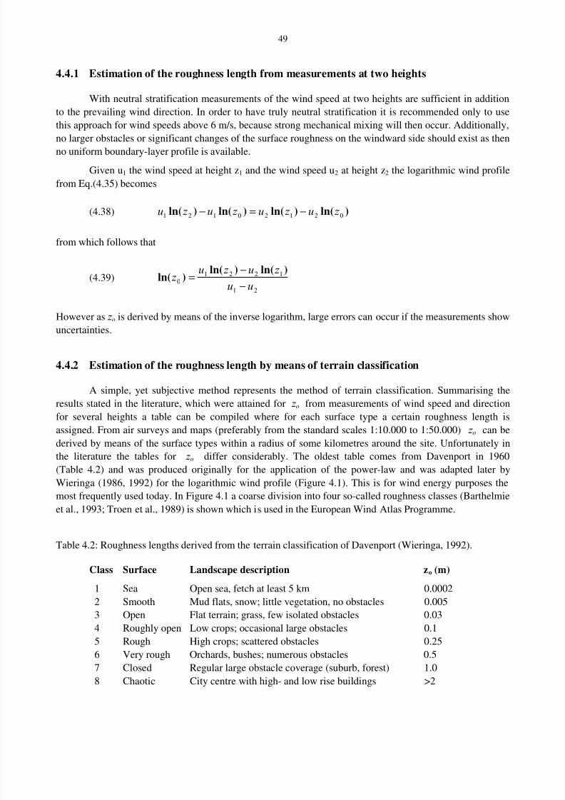
8/2/2019 Dobesch Rpt
http://slidepdf.com/reader/full/dobesch-rpt 55/123
49
4.4.1 Estimation of the roughness length from measurements at two heights
With neutral stratification measurements of the wind speed at two heights are sufficient in addition
to the prevailing wind direction. In order to have truly neutral stratification it is recommended only to use
this approach for wind speeds above 6 m/s, because strong mechanical mixing will then occur. Additionally,
no larger obstacles or significant changes of the surface roughness on the windward side should exist as thenno uniform boundary-layer profile is available.
Given u1 the wind speed at height z1 and the wind speed u2 at height z2 the logarithmic wind profile
from Eq.(4.35) becomes
(4.38) )ln()ln()ln()ln( 02120121 z u z u z u z u −=−
from which follows that
(4.39)21
1221
0 uu
z u z u
z −
−
=
)ln()ln(
)ln(
However as z o is derived by means of the inverse logarithm, large errors can occur if the measurements show
uncertainties.
4.4.2 Estimation of the roughness length by means of terrain classification
A simple, yet subjective method represents the method of terrain classification. Summarising the
results stated in the literature, which were attained for z o from measurements of wind speed and direction
for several heights a table can be compiled where for each surface type a certain roughness length isassigned. From air surveys and maps (preferably from the standard scales 1:10.000 to 1:50.000) z o can be
derived by means of the surface types within a radius of some kilometres around the site. Unfortunately in
the literature the tables for z o differ considerably. The oldest table comes from Davenport in 1960
(Table 4.2) and was produced originally for the application of the power-law and was adapted later by
Wieringa (1986, 1992) for the logarithmic wind profile (Figure 4.1). This is for wind energy purposes the
most frequently used today. In Figure 4.1 a coarse division into four so-called roughness classes (Barthelmie
et al., 1993; Troen et al., 1989) is shown which is used in the European Wind Atlas Programme.
Table 4.2: Roughness lengths derived from the terrain classification of Davenport (Wieringa, 1992).
Class Surface Landscape description zo (m)
1 Sea Open sea, fetch at least 5 km 0.0002
2 Smooth Mud flats, snow; little vegetation, no obstacles 0.005
3 Open Flat terrain; grass, few isolated obstacles 0.03
4 Roughly open Low crops; occasional large obstacles 0.1
5 Rough High crops; scattered obstacles 0.25
6 Very rough Orchards, bushes; numerous obstacles 0.5
7 Closed Regular large obstacle coverage (suburb, forest) 1.0
8 Chaotic City centre with high- and low rise buildings >2
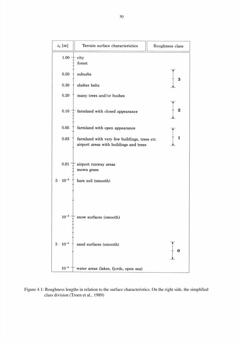
8/2/2019 Dobesch Rpt
http://slidepdf.com/reader/full/dobesch-rpt 56/123
50
Figure 4.1: Roughness lengths in relation to the surface characteristics. On the right side, the simplified
class division (Troen et al., 1989)
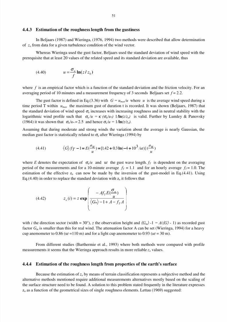
8/2/2019 Dobesch Rpt
http://slidepdf.com/reader/full/dobesch-rpt 57/123
51
4.4.3 Estimation of the roughness length from the gustiness
In Beljaars (1987) and Wieringa, (1976, 1994) two methods were described that allow determination
of z o from data for a given turbulence condition of the wind vector.
Whereas Wieringa used the gust factor, Beljaars used the standard deviation of wind speed with the
prerequisite that at least 20 values of the related speed and its standard deviation are available, thus
(4.40) ) / ln( 0 z z f
u uσ =
where f is an empirical factor which is a function of the standard deviation and the friction velocity. For an
averaging period of 10 minutes and a measurement frequency of 3 seconds Beljaars set f = 2.2.
The gust factor is defined in Eq.(3.36) with G = umax /u where u is the average wind speed during a
time period T within umax the maximum gust of duration t is recorded. It was shown (Beljaars, 1987) that
the standard deviation of wind speed σ u increases with increasing roughness and in neutral stability with thelogarithmic wind profile such that σ u /u = κ ( σ u /u* ) 1 / ln(z/z o ) is valid. Further by Lumley & Panovsky
(1964) it was shown that σ u /u* ≈ 2.5 and hence σ u /u = 1 / ln(z/z o ).
Assuming that during moderate and strong winds the variation about the average is nearly Gaussian, the
median gust factor is statistically related to σ u after Wieringa (1994) by
(4.41) )()]3104(30421[)(1u
uσ
/ut ..u
uσ
E T /f G ++++−−−−++++========−−−− ln
where E denotes the expectation of σ u /u and ut the gust wave length. f T is dependent on the averaging
period of the measurements and for a 10-minute average f T = 1.1 and for an hourly average f T = 1.0. Theestimation of the effective zo can now be made by the inversion of the gust-model in Eq.(4.41). Using
Eq.(4.40) in order to replace the standard deviation with zo it follows that
(4.42)
−+−
−=
A f AG
u E Af
z i z T m
uT
o1
)(
)(
σ
exp
with i the direction sector (width = 30°), z the observation height and ⟨ Gm ⟩ -1 = A(⟨ G ⟩ - 1) as recorded gust
factor Gm is smaller than this for real wind. The attenuation factor A can be set (Wieringa, 1994) for a heavy
cup anemometer to 0.86 (ut =110 m) and for a light cup anemometer to 0.93 (ut = 30 m).
From different studies (Barthermie et al., 1993) where both methods were compared with profile
measurements it seems that the Wieringa approach results in more reliable z o values.
4.4.4 Estimation of the roughness length from properties of the earth’s surface
Because the estimation of z o by means of terrain classification represents a subjective method and the
alternative methods mentioned require additional measurements alternatives mostly based on the scaling of
the surface structure need to be found. A solution to this problem stated frequently in the literature expresses
zo as a function of the geometrical sizes of single roughness elements. Lettau (1969) suggested:
8/2/2019 Dobesch Rpt
http://slidepdf.com/reader/full/dobesch-rpt 58/123
52
(4.43)S
sh z
2
10 =
Where h is the height, s the front surface opposing the wind and S the specific area which results from the
total basis area A and the number of roughness elements n such that S = A/n. Interestingly here however,
only the height and width of the element are included, not their extend in the wind direction. This approach
was examined by Kutzbach (in Oke, 1987), through distributing identical obstacles uniformly across an ice
surface. The comparison with measurements yielded a good agreement proving the included base S was
either not very small or very large.
Figure 4.2: The relative roughness length with respect to the density of obstacles (Oke, 1987)
If the area S is very small the speed becomes virtually zero in the interposed spaces between the
obstacles and the upper sides of the roughness elements which form a new surface with a smaller roughness
as calculated in Eq.(4.43). If S is very large with few obstacles the calculation yields too small a value as the
neglected roughness of the free surface in this case gains more influence.
Kondo et al. (1986) give an approach for non-uniformly distributed roughness elements. The
relevant geometrical height hr for the calculation of z 0 is defined both by the different obstacle heights aswell as the dimension of the intervening free areas:
(4.44) iir g H A
h ∑=1
with A the total area, H i the height and g i the base of the roughness element i. Empirically the following
relationship between z 0 and hr was found:
(4.45) r h z 25.00 =
8/2/2019 Dobesch Rpt
http://slidepdf.com/reader/full/dobesch-rpt 59/123
53
Comparing this approach with that of Lettau for a horizontally uniform ground surface by setting H i = H in
Eq.(4.43), it follows that
(4.46) H
l
S
s H z
4
10 =
where l represents the length of the obstacle in the wind direction. For the particular case of l = 2 H
Eq.(4.43) results.
Raupach (1992) delivers a more complex approach that also takes the height of the displacement
layer thickness into account. He distinguishes between the shear stress of the free surface and that one which
results from differently formed objects. The starting point for consideration is the relationship of z 0 to the
height h of the roughness element in dependence on the dimensionless number q which is defined by the
form and distribution of the roughness elements and their number n occupying the ground area S as
(4.47) S nbhq / =
where b is the width of the roughness element. Existing data show that z 0 /h increases approximately linearly
with q up to a value of 0.1 to 0.15 (where q = qmax from 0.1 to 0.3), but with further increase λ again
decreases. The location of the maximum and the form of the curve described are dependent on the
geometrical form of the obstacles. The existence of a maximum and the decrease of z 0 /h are responsible for
the invalidating Eq.(4.43) for a high density of obstacle elements.
Considering the shear stress within the layer that reaches up to the height of the obstacles the entire
shear stress can be seen as a combination of the shear stress on the ground S τ and that of the roughness
elements τ R:
(4.48) S Ru τ τ ρ τ +== 2
*
This τ is proportional to the air density, a specific drag coefficient of the object and the square of the speed at
height h. Subtracting from these resistance force the shaded surfaces (in the case of the ground surface) and
shaded volumes where bigger than the bases (in the case of the roughness elements), including the volumes
of the roughness elements (as the speed is also zero within an area in the lee of the elements) the entire shear
stress within the layer of thickness h can be written:
(4.49)
−+
−=λ λ ρ τ
**
expexpu
U C C
u
U C C U h
R
h
S h 21
2
where C S is the drag coefficient of the (unobstructed) ground, C R the drag coefficient of an isolated surface-
mounted roughness element and U h as a reference wind speed. It is helpful to consider the constants C 1 and
C 2 as of magnitude 1 and to set them equal. * / uU h is also a function of the shear stress. For the solution of
Eq.(4.49) it can be considered as an implicit function of τ and with * / uU h ≡ γ and C 1 = C 2 = c it follows
that
(4.50) ) / exp()( / 221 γ γ cqqC C RS
−+=
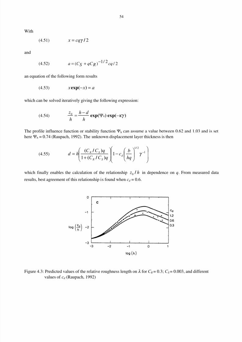
8/2/2019 Dobesch Rpt
http://slidepdf.com/reader/full/dobesch-rpt 60/123
54
With
(4.51) 2 / γ cq x =
and
(4.52) 2 / 2 / 1)( cq RqC S C a −+=
an equation of the following form results
(4.53) a x x =− )exp(
which can be solved iteratively giving the following expression:
(4.54) )exp()exp( κγ −Ψ−
= h
h
d h
h
z 0
The profile influence function or stability function Ψh can assume a value between 0.62 and 1.03 and is set
here Ψh = 0.74 (Raupach, 1992). The unknown displacement layer thickness is then
(4.55)
−
+
= −1
21
11
γ
/
) / (
) / (
hq
bc
qC C
qC C hd d
S R
S R
which finally enables the calculation of the relationship h z / 0 in dependence on q. From measured data
results, best agreement of this relationship is found when cd = 0.6.
Figure 4.3: Predicted values of the relative roughness length on λ for C R = 0.3; C S = 0.003, and different
values of cd (Raupach, 1992)

8/2/2019 Dobesch Rpt
http://slidepdf.com/reader/full/dobesch-rpt 61/123
55
4.5 The vertical wind profile in non-adiabatic stratification
If temperature decreases more strongly with height then in the adiabatic case unstable stratification
occurs as an air parcel which is transported to a higher level if there warmer then its surroundings is
accelerated further due to the inherent lift developed. From this process a reinforcement of the momentum
transport originates and consequently a stronger velocity gradient in the lowermost layer above the grounddevelops than in the adiabatic case. If temperature decreases less with height as in the adiabatic case (or even
increases with height in the case of an inversion) stable stratification results. In this case, the mechanical
momentum transfer is damped and a weaker velocity gradient occurs in the lowermost layer. In order to take
these deviations of the logarithmic wind profile into account it is necessary to formulate an additional term
which describes the dependence of the wind profile on temperature stratification. This can be achieved for
example using. the Monin-Obuchov length (Holtslag, 1984).
4.5.1 The Monin-Obuchov length
The turbulent heat flux is independent of the height under stationary conditions and can be written inthe form.
(4.56) T wcQ p H ′′= ρ
Neglecting the Coriolis force in Eq.(4.15), for a temporal variation of the vertical component w of the wind
speed the buoyancy becomes most influential. A length scale comprising of the three turbulence governing
properties g/T o , u*, and Q H /c p ρ is by dimensional analysis the Monin-Obuchov length L:
(4.57) ) /(**
T wT
g u L ′′
−=κ
3
Because the potential temperature θ is directly proportionally to the temperature, T can be simply
replaced by θ in Eq.(4.57) in order to determine the turbulent heat flux with Eq.(4.14). With stable
stratification the turbulent heat flux is negative in the z-direction and therefore L* >0. With unstable
stratification the turbulent heat flux is positive and therefore L* <0. The velocity gradient for the non-
dimensional function Φ(z/L*) is given by (Holtslag, 1984):
(4.58) *) / (* L z z
u
dz
duΦ=
κ
from which follows in the adiabatic case by comparison with Eq.(4.34) that Φ = 1 which is an important
boundary condition for the determination of the function Φ( z/L*) because in this case the average turbulent
heat flux is zero and therefore z/L*=0.
4.5.2 The vertical profile of wind speed in stable stratification
In the case of stable stratification for the function Φ( z/L*) usually a linear approach is chosen:
(4.59) **) / ( L
z
a L z 11+=Φ
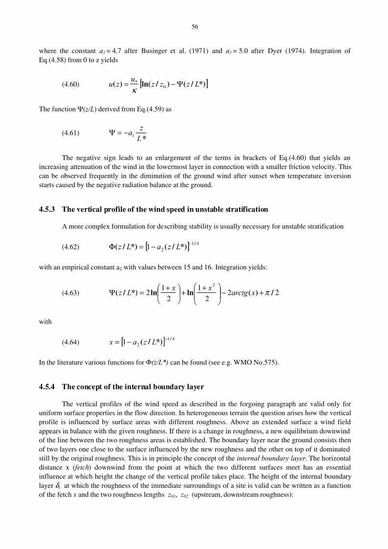
8/2/2019 Dobesch Rpt
http://slidepdf.com/reader/full/dobesch-rpt 62/123
56
where the constant a1 = 4.7 after Businger et al. (1971) and a1 = 5.0 after Dyer (1974). Integration of
Eq.(4.58) from 0 to z yields
(4.60) [ ]*) / () / ln()( * L z z z u
z u Ψ−= 0κ
The function Ψ( z/L) derived from Eq.(4.59) as
(4.61)* L
z a1−=Ψ
The negative sign leads to an enlargement of the terms in brackets of Eq.(4.60) that yields an
increasing attenuation of the wind in the lowermost layer in connection with a smaller friction velocity. This
can be observed frequently in the diminution of the ground wind after sunset when temperature inversion
starts caused by the negative radiation balance at the ground.
4.5.3 The vertical profile of the wind speed in unstable stratification
A more complex formulation for describing stability is usually necessary for unstable stratification
(4.62) [ ] 41
21 /
*) / (*) / (−−=Φ L z a L z
with an empirical constant a2 with values between 15 and 16. Integration yields:
(4.63) 222
12
122
/ )(lnln*) / ( π +−
++
+=Ψ xarctg x x L z
with
(4.64) [ ] 41
21 /
*) / (−−= L z a x
In the literature various functions for Φ(z/L*) can be found (see e.g. WMO No.575).
4.5.4 The concept of the internal boundary layer
The vertical profiles of the wind speed as described in the forgoing paragraph are valid only for
uniform surface properties in the flow direction. In heterogeneous terrain the question arises how the vertical
profile is influenced by surface areas with different roughness. Above an extended surface a wind field
appears in balance with the given roughness. If there is a change in roughness, a new equilibrium downwind
of the line between the two roughness areas is established. The boundary layer near the ground consists then
of two layers one close to the surface influenced by the new roughness and the other on top of it dominated
still by the original roughness. This is in principle the concept of the internal boundary layer . The horizontal
distance x ( fetch) downwind from the point at which the two different surfaces meet has an essential
influence at which height the change of the vertical profile takes place. The height of the internal boundary
layer δ i at which the roughness of the immediate surroundings of a site is valid can be written as a function
of the fetch x and the two roughness lengths z 01, z 02 (upstream, downstream roughness):
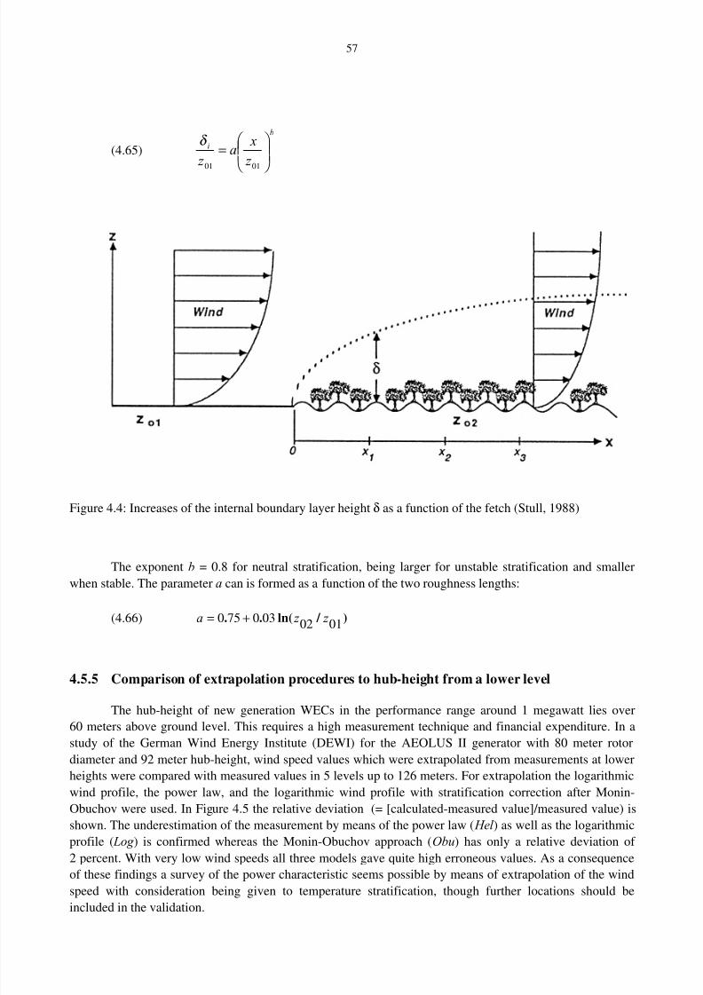
8/2/2019 Dobesch Rpt
http://slidepdf.com/reader/full/dobesch-rpt 63/123
57
(4.65)
b
i
z
xa
z
=
0101
δ
Figure 4.4: Increases of the internal boundary layer height δ as a function of the fetch (Stull, 1988)
The exponent b = 0.8 for neutral stratification, being larger for unstable stratification and smaller
when stable. The parameter a can is formed as a function of the two roughness lengths:
(4.66) ) / ln(..0102030750 z z a +=
4.5.5 Comparison of extrapolation procedures to hub-height from a lower level
The hub-height of new generation WECs in the performance range around 1 megawatt lies over
60 meters above ground level. This requires a high measurement technique and financial expenditure. In a
study of the German Wind Energy Institute (DEWI) for the AEOLUS II generator with 80 meter rotor
diameter and 92 meter hub-height, wind speed values which were extrapolated from measurements at lower
heights were compared with measured values in 5 levels up to 126 meters. For extrapolation the logarithmic
wind profile, the power law, and the logarithmic wind profile with stratification correction after Monin-
Obuchov were used. In Figure 4.5 the relative deviation (= [calculated-measured value]/measured value) is
shown. The underestimation of the measurement by means of the power law ( Hel ) as well as the logarithmic
profile ( Log ) is confirmed whereas the Monin-Obuchov approach (Obu) has only a relative deviation of
2 percent. With very low wind speeds all three models gave quite high erroneous values. As a consequence
of these findings a survey of the power characteristic seems possible by means of extrapolation of the windspeed with consideration being given to temperature stratification, though further locations should be
included in the validation.
8/2/2019 Dobesch Rpt
http://slidepdf.com/reader/full/dobesch-rpt 64/123
58
wind speed
Figure 4.5: Average relative deviation over the measured wind speed at a height of 92 meters;
for annotation see text (Strack et al., 1996)
4.6 The representativeness of wind measurements
It is a fact that wind measurements at 10 meters height are very often corrupted by the specific
surroundings of the measuring site. Hence the question arises are such measurements “climatologically“
representative and the data can be used equally optimal for different purposes. We know well the regulations
for anemometer measurements (WMO No.8, VI.6.6. 1973): "Measurements of wind for synoptic purposes
should refer to a height of 10m in an unobstructed area, and should consist of the mean of values taken over
a period of about 10 minutes". And further on for non-ideal sites: „When a standard exposure is
unobtainable, the anemometer should be installed at such a height that its indications are reasonablyunaffected by local obstructions in the vicinity. This will usually necessitate placing the anemometer at a
height exceeding 10m by an amount depending on the extent, height and distance of the obstructions, but it is
impracticable to give any general rule for determining this since local conditions differ so widely“.
The definition of representativeness is difficult due to the applications that may have their own
conditions in time and space for which then the data have to be representative (Wieringa, 1994). This
imposes that some kind of generalisation is necessary to achieve a regional representativeness that holds for
different applications.
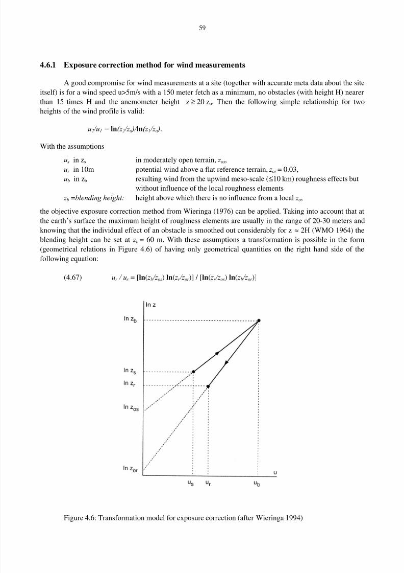
8/2/2019 Dobesch Rpt
http://slidepdf.com/reader/full/dobesch-rpt 65/123
59
4.6.1 Exposure correction method for wind measurements
A good compromise for wind measurements at a site (together with accurate meta data about the site
itself) is for a wind speed u>5m/s with a 150 meter fetch as a minimum, no obstacles (with height H) nearer
than 15 times H and the anemometer height z ≥ 20 zo. Then the following simple relationship for twoheights of the wind profile is valid:
u2 /u1 = ln(z 2 /z o )/ ln(z 1 /z o ).
With the assumptions
u s in zs in moderately open terrain, z os,
ur in 10m potential wind above a flat reference terrain, z or = 0.03,
ub in zb resulting wind from the upwind meso-scale (≤10 km) roughness effects but
without influence of the local roughness elements
z b =blending height: height above which there is no influence from a local z o,the objective exposure correction method from Wieringa (1976) can be applied. Taking into account that at
the earth’s surface the maximum height of roughness elements are usually in the range of 20-30 meters and
knowing that the individual effect of an obstacle is smoothed out considerably for z ≈ 2H (WMO 1964) the
blending height can be set at z b = 60 m. With these assumptions a transformation is possible in the form
(geometrical relations in Figure 4.6) of having only geometrical quantities on the right hand side of the
following equation:
(4.67) ur / u s = [ln( z b /z os) ln( z r /z or )] / [ln( z s /z os) ln( z b /z or )]
Figure 4.6: Transformation model for exposure correction (after Wieringa 1994)

8/2/2019 Dobesch Rpt
http://slidepdf.com/reader/full/dobesch-rpt 66/123
60
The advantages in using the potential wind instead of original wind data are -„standardisation“ of so
called „design values“ and having representative input data for models and other applications. The
disadvantages are that the procedure is applicable only for well kept stations with detailed information about
the surroundings, that homogenisation of the series is necessary in case the station is moved to another site
or changing surroundings and for wind speeds u>5 m/s.

8/2/2019 Dobesch Rpt
http://slidepdf.com/reader/full/dobesch-rpt 67/123
61
5 FLOW FIELDS AND OROGRAPHY
Inhomogeneous terrain formations can change the wind field in comparison with a homogenous
surface in two ways. Firstly, a change in the pressure field can be evoked dynamically by the orography on
an existing flow and secondly, pressure gradients can be generated, even in wind still periods, at the upperlevel of the boundary layer caused by thermally induced winds from varying energy absorption of the earth’s
surface depending on hillside inclination and orientation - the so-called thermal induced winds. The first part
of this section deals with the influence of topographic elevations on a flow which results from the spatial
pressure distribution, the second part with thermally induced flows.
5.1 Flows over and around hills
Flows above and around elevations are strongly dependent on the height and shape of the hill or
mountain, as well as the velocity of flow and prevailing temperature stratification. The different flow forms
can be distinguished by the resultant forces to be considered. Firstly some characteristic properties of the
flow and atmosphere are discussed.
5.1.1 The Brunt-Väisälä frequency and the atmospheric wavelength
If an air parcel is lifted in a stable stratified flow a restoring force is generated that tries to bring back
the parcel to the original location caused by differential buoyancy of the air parcel and its surroundings. On
the basis of this restitution force oscillations of the air parcel occur in the vertical with the so-called Brunt-
Väisälä or buoyancy frequency (Stull, 1988; Holton 1992):
(5.1)
2 / 1
=
dz
d g N f
θ
θ
where θ (z) is the potential temperature at the original position z. If a stable stratified flow is lifted with the
speed u by a hill or mountain then in front, above and behind this elevation waves are formed. The
atmospheric wavelength λ a results from the Brunt-Väisälä frequency and the flow velocity u as
(5.2) f
a N
uπ λ 2=
Taking an average value of 0.0035 K/m for the vertical gradient of the potential temperature an average
value and for the velocity u = 10 m/s the atmospheric wavelength emerges as approximately 5 kilometres.
Which wave form develops during the flow over the mountain is dependent on the relationship of the
characteristic horizontal extend L of the mountain to the atmospheric wavelength
(5.3)u
N L L f
a ⋅⋅
=π λ 50.

8/2/2019 Dobesch Rpt
http://slidepdf.com/reader/full/dobesch-rpt 68/123
62
5.1.2 Wave regimes of flows over hills
The following considerations will focus for simplicity on two-dimensional elevations such that the
wind vector has only two components u and w. Concentrating only on mountain ranges limited laterally, the
effects resulting from Coriolis acceleration can be neglected. Starting with the boundary layer equations and
the non-averaged Boussinesq-approximation (Holton, 1992) (c.f. paragraph 4.2.7) without the Coriolis termwe have
(5.4)du
dt
p
x= −
1
ρ
∂
∂
(5.5)dw
dt
p
zg= − −
1
ρ
∂
∂
(5.6)d
dt
θ = 0
and using continuity equation for an incompressible medium (cf. Eq.4.4) the governing equations for the
deviation from the basic state are obtained by use of Reynolds averaging and linearisation, neglecting effects
of rotation yields:
(5.7)∂
∂
∂
∂ ρ
∂
∂ tu
xu
p
x+
′ +
′=
10
0
(5.8)∂
∂
∂
∂ ρ
∂
∂
θ
θ tu
xw
p
zg+
′ +
′−
′=
10
0
(5.9)∂
∂
∂
∂
′+
′=
u
x
w
z0
(5.10)
∂
∂
∂
∂ θ
θ
t u x w
d
dz+
′ + ′ = 0
Eliminating the pressure disturbance by subtracting Eq.(5.7) from Eq.(5.8), and subsequently u´ and θ with
the help of Eqs.(5.9) and (5.10) one derives the conditional equation for w''
(5.11) 02
22
2
2
2
22
=′
+
′+
′
+
x
w N
z
w
x
w
xu
t f
∂
∂
∂
∂
∂
∂
∂
∂
∂
∂
This wave equation describes the so-called internal gravity waves in the general form also allowing for
temporal changes. In the case of flowing over high mountains this temporal change is not possible andstationary wave are formed (Holton, 1992), because of the average horizontal wind speed and terrain height
(the cause for the flow lifting) being constant. Therefore Eq.(5.11) simplifies to

8/2/2019 Dobesch Rpt
http://slidepdf.com/reader/full/dobesch-rpt 69/123
63
(5.12) 02
2
2
2
2
2
=′+′
+′
wu
N
z
w
x
w f
∂
∂
∂
∂
Parts of this equation can be neglected according to the horizontal extend of elevation. For hills, whose
length is smaller than the atmospheric wavelength in flow direction, no waves develop and the third term in
Eq.(5.12), responsible for wave development, can be neglected. The remaining terms yield the Laplace-
Equation
(5.13) 02
2
2
2
=′∆=′
+′
w z
w
x
w
∂
∂
∂
∂
This form results from the requirement that the gradient field of a scalar potential (in this case the vertical
deflection), that fulfils the non-vortical condition, must also be non-divergent. Therefore, flows that fulfil the
Laplace equation are named potential flows. As these flows are also valid in the case of stable stratification
the solutions for Eq.(5.13) will be discussed in section 5.1.4.
In the case that the horizontal extent of the hill reaches approximately the atmospheric wavelength a
non-hydrostatic wave regime is established and all terms in Eq.(5.12) must be considered. Then waves are
generated which extend themselves in the horizontal and vertical directions also. The harmonic wave
solution of Eq.(5.11) for the decay or growth of the vertical deflection in relation to x and z has the form
(5.14) Φ−Φ=Φ=′ sincos)]exp(Re[),( ir wwiw z xw!
with w !
a complex amplitude having a real part r w and an imaginary part iw . The phase Φ is a linear
combination of x and z and can be written as
(5.15) mz kx +=Φ
with k the wave number in the x–direction and m the wave number in the z-direction. While the horizontal
wave number is always real and therefore in the x-direction has sine-shaped waves forms, the vertical wave
number m = mr + mi may be complex so that in this case an exponential decay or growth of the vertical
deflection takes place depending on whether mi is positive or negative. The differentiation, if sine-shaped
waves developed vertically direction or if an exponential decay or growth occurs, results from the so-called
dispersion relationship:
(5.16)
2222
k u N m −= /
If the horizontal velocity of flow is smaller than the ratio of Brunt-Väisälä frequency to the horizontal wave-
number, m is real and waves are generated in the z-direction. In this case the lines, which can be drawn
through points at different heights with the same phase, are not vertical but deflected from the local vertical
through an angle α (Blumen, 1990). The cosine of this angle results from the ratio of the horizontal wave
number to the amount of the wave number vector thus
(5.17)→
±= k k / cosα
where the wave number vector has the x-component k and the z-component m. The tilt of the phase lines for
internal gravity waves depends only on the ratio of the wave frequency to the buoyancy frequency and is
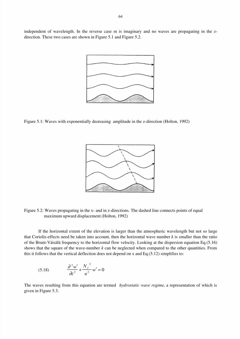
8/2/2019 Dobesch Rpt
http://slidepdf.com/reader/full/dobesch-rpt 70/123
64
independent of wavelength. In the reverse case m is imaginary and no waves are propagating in the z-
direction. These two cases are shown in Figure 5.1 and Figure 5.2.
Figure 5.1: Waves with exponentially decreasing amplitude in the z-direction (Holton, 1992)
Figure 5.2: Waves propagating in the x- and in z-directions. The dashed line connects points of equal
maximum upward displacement (Holton, 1992)
If the horizontal extent of the elevation is larger than the atmospheric wavelength but not so large
that Coriolis-effects need be taken into account, then the horizontal wave number k is smaller than the ratioof the Brunt-Väisälä frequency to the horizontal flow velocity. Looking at the dispersion equation Eq.(5.16)
shows that the square of the wave-number k can be neglected when compared to the other quantities. From
this it follows that the vertical deflection does not depend on x and Eq.(5.12) simplifies to:
(5.18) 02
2
2
2
=′+′
wu
N
z
w f
∂
∂
The waves resulting from this equation are termed hydrostatic wave regime, a representation of which is
given in Figure 5.3.
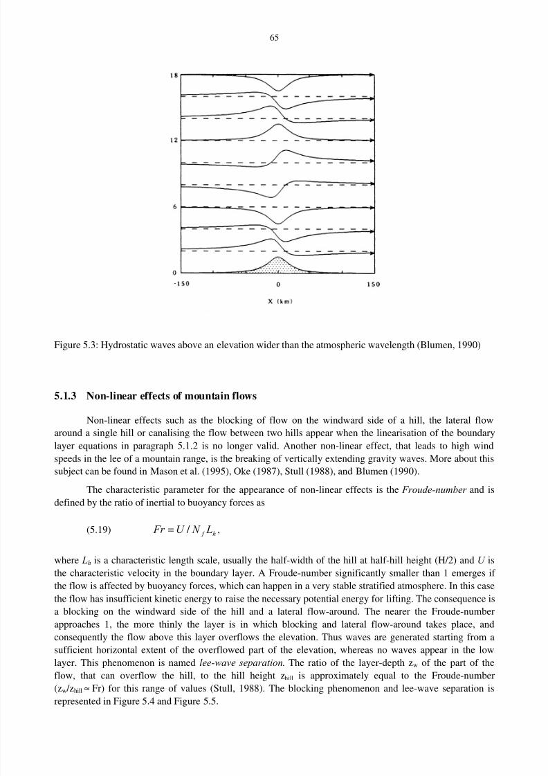
8/2/2019 Dobesch Rpt
http://slidepdf.com/reader/full/dobesch-rpt 71/123
65
Figure 5.3: Hydrostatic waves above an elevation wider than the atmospheric wavelength (Blumen, 1990)
5.1.3 Non-linear effects of mountain flows
Non-linear effects such as the blocking of flow on the windward side of a hill, the lateral flow
around a single hill or canalising the flow between two hills appear when the linearisation of the boundary
layer equations in paragraph 5.1.2 is no longer valid. Another non-linear effect, that leads to high wind
speeds in the lee of a mountain range, is the breaking of vertically extending gravity waves. More about this
subject can be found in Mason et al. (1995), Oke (1987), Stull (1988), and Blumen (1990).
The characteristic parameter for the appearance of non-linear effects is the Froude-number and is
defined by the ratio of inertial to buoyancy forces as
(5.19) h f L N U Fr / = ,
where Lh is a characteristic length scale, usually the half-width of the hill at half-hill height (H/2) and U is
the characteristic velocity in the boundary layer. A Froude-number significantly smaller than 1 emerges if
the flow is affected by buoyancy forces, which can happen in a very stable stratified atmosphere. In this case
the flow has insufficient kinetic energy to raise the necessary potential energy for lifting. The consequence is
a blocking on the windward side of the hill and a lateral flow-around. The nearer the Froude-number
approaches 1, the more thinly the layer is in which blocking and lateral flow-around takes place, and
consequently the flow above this layer overflows the elevation. Thus waves are generated starting from a
sufficient horizontal extent of the overflowed part of the elevation, whereas no waves appear in the low
layer. This phenomenon is named lee-wave separation. The ratio of the layer-depth zw of the part of the
flow, that can overflow the hill, to the hill height zhill is approximately equal to the Froude-number(zw /zhill ≈ Fr) for this range of values (Stull, 1988). The blocking phenomenon and lee-wave separation is
represented in Figure 5.4 and Figure 5.5.
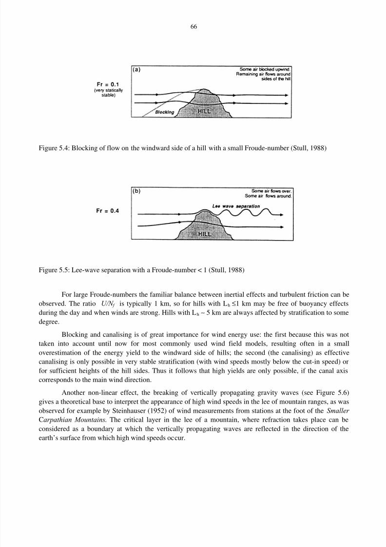
8/2/2019 Dobesch Rpt
http://slidepdf.com/reader/full/dobesch-rpt 72/123
66
Figure 5.4: Blocking of flow on the windward side of a hill with a small Froude-number (Stull, 1988)
Figure 5.5: Lee-wave separation with a Froude-number < 1 (Stull, 1988)
For large Froude-numbers the familiar balance between inertial effects and turbulent friction can be
observed. The ratio U/N f is typically 1 km, so for hills with Lh ≤1 km may be free of buoyancy effects
during the day and when winds are strong. Hills with Lh ∼ 5 km are always affected by stratification to some
degree.
Blocking and canalising is of great importance for wind energy use: the first because this was not
taken into account until now for most commonly used wind field models, resulting often in a small
overestimation of the energy yield to the windward side of hills; the second (the canalising) as effective
canalising is only possible in very stable stratification (with wind speeds mostly below the cut-in speed) or
for sufficient heights of the hill sides. Thus it follows that high yields are only possible, if the canal axis
corresponds to the main wind direction.Another non-linear effect, the breaking of vertically propagating gravity waves (see Figure 5.6)
gives a theoretical base to interpret the appearance of high wind speeds in the lee of mountain ranges, as was
observed for example by Steinhauser (1952) of wind measurements from stations at the foot of the Smaller
Carpathian Mountains. The critical layer in the lee of a mountain, where refraction takes place can be
considered as a boundary at which the vertically propagating waves are reflected in the direction of the
earth’s surface from which high wind speeds occur.
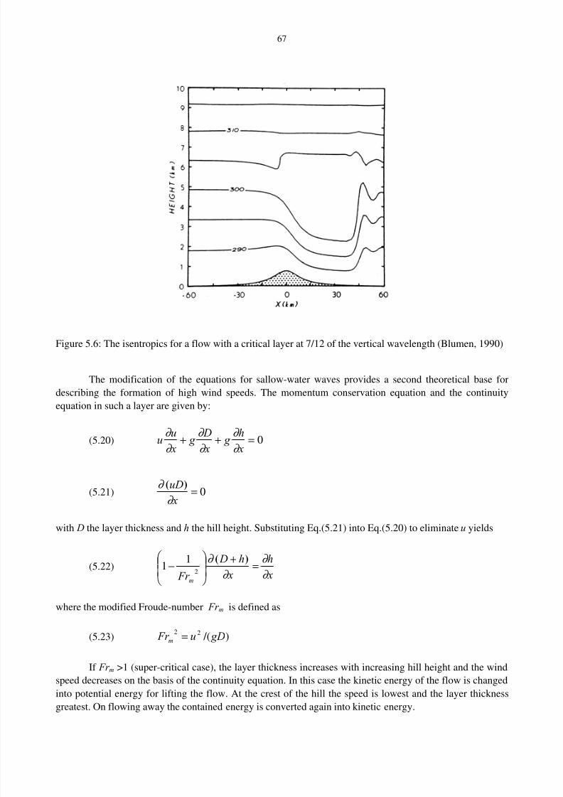
8/2/2019 Dobesch Rpt
http://slidepdf.com/reader/full/dobesch-rpt 73/123
67
Figure 5.6: The isentropics for a flow with a critical layer at 7/12 of the vertical wavelength (Blumen, 1990)
The modification of the equations for sallow-water waves provides a second theoretical base for
describing the formation of high wind speeds. The momentum conservation equation and the continuity
equation in such a layer are given by:
(5.20) 0=++ x
h g
x
D g
x
uu
∂
∂
∂
∂
∂
∂
(5.21) 0= x
uD
∂
∂ )(
with D the layer thickness and h the hill height. Substituting Eq.(5.21) into Eq.(5.20) to eliminate u yields
(5.22) xh
xh D
Fr m ∂ ∂
∂ ∂ =+
− )(
211
where the modified Froude-number Fr m is defined as
(5.23) ) /(22 gDu Fr m =
If Fr m >1 (super-critical case), the layer thickness increases with increasing hill height and the wind
speed decreases on the basis of the continuity equation. In this case the kinetic energy of the flow is changed
into potential energy for lifting the flow. At the crest of the hill the speed is lowest and the layer thicknessgreatest. On flowing away the contained energy is converted again into kinetic energy.
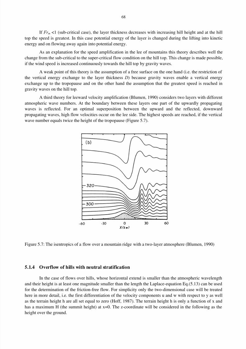
8/2/2019 Dobesch Rpt
http://slidepdf.com/reader/full/dobesch-rpt 74/123
68
If Fr m <1 (sub-critical case), the layer thickness decreases with increasing hill height and at the hill
top the speed is greatest. In this case potential energy of the layer is changed during the lifting into kinetic
energy and on flowing away again into potential energy.
As an explanation for the speed amplification in the lee of mountains this theory describes well the
change from the sub-critical to the super-critical flow condition on the hill top. This change is made possible,
if the wind speed is increased continuously towards the hill top by gravity waves.
A weak point of this theory is the assumption of a free surface on the one hand (i.e. the restriction of
the vertical energy exchange to the layer thickness D) because gravity waves enable a vertical energy
exchange up to the tropopause and on the other hand the assumption that the greatest speed is reached in
gravity waves on the hill top.
A third theory for leeward velocity amplification (Blumen, 1990) considers two layers with different
atmospheric wave numbers. At the boundary between these layers one part of the upwardly propagating
waves is reflected. For an optimal superposition between the upward and the reflected, downward
propagating waves, high flow velocities occur on the lee side. The highest speeds are reached, if the vertical
wave number equals twice the height of the tropopause (Figure 5.7).
Figure 5.7: The isentropics of a flow over a mountain ridge with a two-layer atmosphere (Blumen, 1990)
5.1.4 Overflow of hills with neutral stratification
In the case of flows over hills, whose horizontal extend is smaller than the atmospheric wavelength
and their height is at least one magnitude smaller than the length the Laplace-equation Eq.(5.13) can be used
for the determination of the friction-free flow. For simplicity only the two-dimensional case will be treated
here in more detail, i.e. the first differentiation of the velocity components u and w with respect to y as well
as the terrain height h are all set equal to zero (Hoff, 1987). The terrain height h is only a function of x and
has a maximum H (the summit height) at x=0. The z-coordinate will be considered in the following as theheight over the ground.
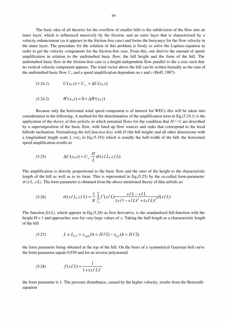
8/2/2019 Dobesch Rpt
http://slidepdf.com/reader/full/dobesch-rpt 75/123
69
The basic idea of all theories for the overflow of smaller hills is the subdivision of the flow into an
inner layer, which is influenced massively by the friction, and an outer layer that is characterised by a
velocity enhancement (as it appears in the friction-free case) and forms the buoyancy for the flow velocity in
the inner layer. The procedure for the solution of this problem is firstly to solve the Laplace-equation in
order to get the velocity components for the friction-free case. From this, one derives the amount of speed
amplification in relation to the undisturbed basic flow, the hill height and the form of the hill. Theundisturbed basic flow in the friction-free case is a height-independent flow parallel to the x-axis such that
no vertical velocity component appears. The wind vector above the hill can be written formally as the sum of
the undisturbed basic flow U ∞ and a speed amplification dependent on x and z (Hoff, 1987):
(5.24.1) ),(),( z xU U z xU ∆+= ∞
(5.24.2) ),(),( z xW z xW ∆+= 0
Because only the horizontal wind speed component is of interest for WECs this will be taken intoconsideration in the following. A method for the determination of the amplification term in Eq.(5.24.1) is the
application of the theory of thin airfoils, in which potential flows for the condition that H<<L are described
by a superimposition of the basic flow, with lined up flow sources and sinks that correspond to the local
hillside inclination. Normalising the hill-function h(x) with H (the hill height) and all other dimensions with
a longitudinal length scale L (= Lh in Eq.(5.19)) which is usually the half-width of the hill, the horizontal
speed amplification results in:
(5.25) ) / , / (),( L z L x L
H U z xU σ ∞=∆
The amplification is directly proportional to the basic flow and the ratio of the height to the characteristic
length of the hill as well as to its form. This is represented in Eq.(5.25) by the so-called form-parameter
σ (x/L, z/L). The form parameter is obtained from the above mentioned theory of thin airfoils as:
(5.26) ) / () / () / / (
/ / ) / () / , / ( L sd
L z L sl x
L s L x L s f L z L x ∫
∞
∞− +−−′=
22
1
π σ
The function f(x/L), which appears in Eq.(5.26) as first derivative, is the standardised hill-function with the
height H = 1 and approaches zero for very large values of x. Taking the half-length as a characteristic length
of the hill
(5.27) ) / () / ( / 2221 H h x H h x L L left right =−==≡
the form parameter being obtained at the top of the hill. On the basis of a symmetrical Gaussian bell curve
the form parameter equals 0.939 and for an inverse polynomial
(5.28)21
1
) / () / (
L x L x f
+=
the form parameter is 1. The pressure disturbance, caused by the higher velocity, results from the Bernoulli-equation
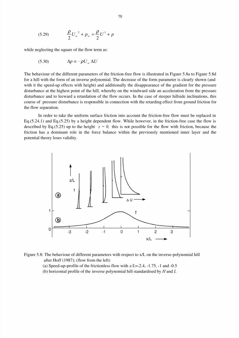
8/2/2019 Dobesch Rpt
http://slidepdf.com/reader/full/dobesch-rpt 76/123
70
(5.29) pU pU +=+ ∞∞22
22
ρ ρ
while neglecting the square of the flow term as:
(5.30) U U p ∆−≅∆ ∞ρ
The behaviour of the different parameters of the friction-free flow is illustrated in Figure 5.8a to Figure 5.8d
for a hill with the form of an inverse polynomial. The decrease of the form parameter is clearly shown (and
with it the speed-up effects with height) and additionally the disappearance of the gradient for the pressure
disturbance at the highest point of the hill, whereby on the windward side an acceleration from the pressure
disturbance and to leeward a retardation of the flow occurs. In the case of steeper hillside inclinations, this
course of pressure disturbance is responsible in connection with the retarding effect from ground friction for
the flow separation.
In order to take the uniform surface friction into account the friction-free flow must be replaced in
Eq.(5.24.1) and Eq.(5.25) by a height dependent flow. While however, in the friction-free case the flow is
described by Eq.(5.25) up to the height z = 0, this is not possible for the flow with friction, because the
friction has a dominant role in the force balance within the previously mentioned inner layer and the
potential theory loses validity.
Figure 5.8: The behaviour of different parameters with respect to x/L on the inverse-polynomial hill
after Hoff (1987); (flow from the left)
(a) Speed-up-profile of the frictionless flow with x/L=-2.4, -1.75, -1 and -0.5
(b) horizontal profile of the inverse polynomial hill standardised by H and L
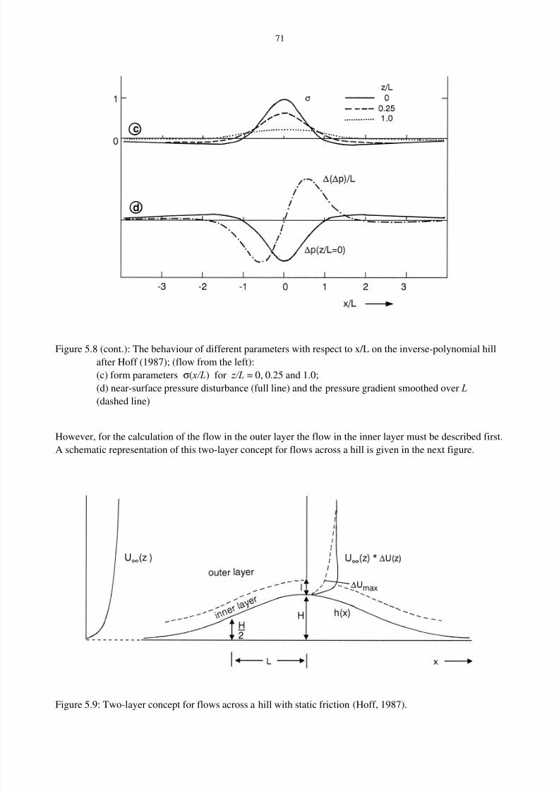
8/2/2019 Dobesch Rpt
http://slidepdf.com/reader/full/dobesch-rpt 77/123
71
Figure 5.8 (cont.): The behaviour of different parameters with respect to x/L on the inverse-polynomial hill
after Hoff (1987); (flow from the left):
(c) form parameters σ( x/L) for z/L = 0, 0.25 and 1.0;
(d) near-surface pressure disturbance (full line) and the pressure gradient smoothed over L
(dashed line)
However, for the calculation of the flow in the outer layer the flow in the inner layer must be described first.
A schematic representation of this two-layer concept for flows across a hill is given in the next figure.
Figure 5.9: Two-layer concept for flows across a hill with static friction (Hoff, 1987).

8/2/2019 Dobesch Rpt
http://slidepdf.com/reader/full/dobesch-rpt 78/123
72
With the application of the logarithmic wind profile from Eq.(4.35) the solution for the speed
amplification in the outer layer which lies above the inner layer with the still unknown layer-thickness l is
given by
(5.31) ) / , / ()()(),( L z L x L
H
LU z U z xU σ ∞∞ +=
As scaling velocity for the horizontal speed increases, the velocity was chosen for the height H , which
represents the typical effect height of the obstacle.
For the flow around hills the relevant forces are, as mentioned above, advection, pressure gradient
and friction. The pressure gradient directly on the ground must be equal to the friction, because for advection
the necessary velocity vanishes here. Under the assumption that the pressure disturbance is hardly modified
by the inner friction layer, the required layer thickness l' of the inner layer can be gained from equating the
change of the shear stress ∆τ within the depth l' with the advection at the lower boundary of the outer
layer:
(5.32)'
)'()'(
l L
l U l U
τ
ρ
∆=
∆∞
1
If one uses the shear stress velocity instead of the friction velocity, the right hand side of Eq.(5.32) is given
after splitting off the friction velocity into an undisturbed term and an additional term, with a subsequent
linearisation as:
(5.33)''
)( **
*
l
uu
l
u ∆≅
∆∞2
2
Using for the undisturbed term
(5.34)) / 'ln(
)'(*
0 z l l U u
κ ∞∞ =
and for the disturbed term
(5.35)
) / 'ln(
)'(*
0 z l
l U uκ
∆=∆
after some reshaping the conditional equation for the layer thickness l' this becomes:
(5.36) L z l l 2
0
2 2κ =⋅ ) / '(ln'
Beside this equation there are others in the literature (Hunt et al., 1975; Britter et al., 1981) for which the
logarithm is not squared as e.g.
(5.37) L z l l 2
0 2κ =⋅ ) / 'ln(' ,
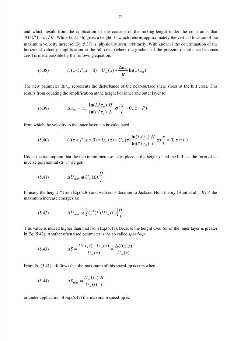
8/2/2019 Dobesch Rpt
http://slidepdf.com/reader/full/dobesch-rpt 79/123
73
and which result from the application of the concept of the mixing-length under the constraints that
κ / )'( *ul U =∆ . While Eq.(5.36) gives a height l' which returns approximately the vertical location of the
maximum velocity increase, Eq.(5.37) is, physically seen, arbitrarily. With known l the determination of the
horizontal velocity amplification at the hill crest (where the gradient of the pressure disturbance becomes
zero) is made possible by the following equation:
(5.38) ) / ln()(),'( *0
00 z z u
z U xl z U κ
∆+==< ∞
The new parameter 0*u∆ represents the disturbance of the near-surface shear stress at the hill crest. This
results from equating the amplification at the height l of inner and outer layer to
(5.39) )',() / 'ln(
) / ln(** l z
L
x
L
H
z l
z Luu ===∆ ∞ 0
0
00 σ
from which the velocity in the inner layer can be calculated:
(5.40) )',() / 'ln(
) / ln()()(),'( l z
L
x
L
H
z l
z L z U z U xl z U ==+==< ∞∞ 00
0
0 σ
Under the assumption that the maximum increase takes place at the height l' and the hill has the form of an
inverse polynomial (σ=1) we get:
(5.41) L
H
LU U )(max ∞≅∆
In using the height l' from Eq.(5.36) and with consideration to Jackson-Hunt theory (Hunt et al., 1975) the
maximum increase emerges as:
(5.42) [ ] L
H l U LU U )'( / )(max ∞∞≅∆ 2
This value is indeed higher than that from Eq.(5.41), because the height used for of the inner layer is greater
in Eq.(5.42). Another often used parameter is the so called speed-up:
(5.43))(
),(
)(
)(),(
z U
z xU
z U
z U z xU S
∞∞
∞ ∆=
−=∆
From Eq.(5.41) it follows that the maximum of this speed-up occurs when
(5.44) L
H
l U
LU S
e
)(
)(max
∞
∞=∆
or under application of Eq.(5.42) the maximum speed-up is:
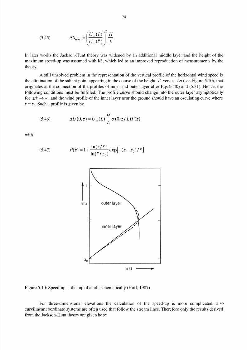
8/2/2019 Dobesch Rpt
http://slidepdf.com/reader/full/dobesch-rpt 80/123
74
(5.45) L
H
l U
LU S
2
=∆
∞
∞
)'(
)(max
In later works the Jackson-Hunt theory was widened by an additional middle layer and the height of the
maximum speed-up was assumed with l/3, which led to an improved reproduction of measurements by thetheory.
A still unsolved problem in the representation of the vertical profile of the horizontal wind speed is
the elimination of the salient point appearing in the course of the height l' versus ∆u (see Figure 5.10), that
originates at the connection of the profiles of inner and outer layer after Eqs.(5.40) and (5.31). Hence, the
following conditions must be fulfilled: The profile curve should change into the outer layer asymptotically
for z/l' → ∞ and the wind profile of the inner layer near the ground should have an osculating curve where
z = z 0. Such a profile is given by
(5.46) )() / ,()(),( z P L z L
H LU z U 00 σ ∞=∆
with
(5.47) [ ]' / )(exp) / 'ln(
)' / ln()( l z z
z l
l z z P 0
0
1 −−+=
Figure 5.10: Speed-up at the top of a hill, schematically (Hoff, 1987)
For three-dimensional elevations the calculation of the speed-up is more complicated, also
curvilinear coordinate systems are often used that follow the stream lines. Therefore only the results derived
from the Jackson-Hunt theory are given here:
8/2/2019 Dobesch Rpt
http://slidepdf.com/reader/full/dobesch-rpt 81/123
75
(5.48.1) L H S / .max 61≅∆ for axis-symmetrical hills
(5.48.2) L H S / .max 80≅∆ for 2-dimensional terrain steps
(5.48.3) L H S / .max 02≅∆ for 2-dimensional mountain ridges
However, these equations lose their validity if the hillside inclination becomes too large. In this case a region
forms with separate flow in the lee of the highest point a region forms with separated flow (see paragraph
5.1.3). While in the above equations the pressure field is derived from the form of the hill, during flow-
separation the region beneath the flow-separation must be considered in addition to the true elevation for the
calculation of the pressure field, which leads to a shift of the summit into the windward side and to an
elongation of the horizontal extension of the overflowed structure. By the shift of the geographically highest
point to the windward side three-dimensional, axis-symmetrical hills with large hillside inclinations reach for
example a maximum speed-up of only 1.25 H/L (Bradley et al., 1986).The horizontal extent of the so-called separation-bubble includes all points of h(x), for which
(5.49) 00
<= z z
U
∂
∂
is valid. This happens specifically when the flow to the wind ward side is slowed down in the acceleration
region by friction such that overcoming the positive pressure gradient by the flow is no longer possible
behind the highest point. As a consequence the smaller the ratio of the hill height to the roughness length is,
the sooner a flow-separation appears in the lee. Another important criterion for the appearance of flow-
separation is the hillside inclination represented as a measure of adequate approximation
Figure 5.11: Flow separation with respect to hill height and hillside inclination (Petersen 1990)
8/2/2019 Dobesch Rpt
http://slidepdf.com/reader/full/dobesch-rpt 82/123
76
for the curvature of the pressure disturbance with respect to x. The stronger the increase of the positive, lee
side pressure gradient is (see Figure 5.8.d), the more difficult becomes to overcome, such that in the case of
a sharp edged hill crest (which is equal to an infinitely large curvature of the pressure disturbance) flow-
separation always appears. The dependence of flow-separation on the two mentioned causes is shown in
Figure 5.11. It follows that flow-separation appears for a given roughness length and hillside inclination of
10 to 20 degrees or more.
There are two possibilities for testing the theoretical findings: Firstly, a large-scale field experiment
with high technical and consequent financial expenditure, secondly, a wind-tunnel experiment. While for the
first case, discovering a suitably formed hill with uniform surface roughness over a distance of
approximately 5 kilometres would be difficult, in the second case it is realising a ratio of the hill height to
roughness length. Because in wind tunnel hill heights of only one to two meters can be reached the
roughness must be scaled for a realistic model of the flow conditions and consequently, has to be very small.
This leads to the problem that for inferior roughness no realistic turbulent boundary layer is formed,
therefore flow investigations in the wind tunnels are usually restricted to the case of forested hills which are
of little use for wind energy purposes (Britter et al., 1981).
Extensive and well documented field experiments were performed e.g. in Scotland at the AskerveinHill (Walmsley et al., 1996), in Australia on the Black Mountain and in Canada at Kettles Hill (see Taylor et
al., 1987). While Askervein Hill and Kettles Hill have only very low roughness, the Black Mountain is
forested (Table 5.1). All three hills are approximately two dimensional, i.e. the length of the hill is
essentially smaller than the width (Bradley et al., 1986; Hoff, 1987).
The results of these field experiments confirm in the case of low roughness the validity of Eq.(5.36)
for the height of the inner layer and the maximum velocity increase. Only the forested Black Mountain
delivers a layer-thickness l, which corresponds to Eq.(5.37). But this could be explained by the very steep
hill and possibly separated flow in the lee falsifying the results. A summary of the results of all three field
experiments with theoretical calculations for comparison is given the following table.
Table 5.1: Comparison of the layer thickness l' from theory with measured values humax (all parameters in m);
after Bradley (1986)
Field experiment Roughness Height H L l'* l'** maxuh
Black Mountain 1.14 170 275 28 14 27
Askervein Hill 0.03 116 215 12 3.2 3
Kettles Hill 0.01 100 520 22 4.5 5
(*) after Eq.(5.37); (**) after Eq.(5.36)
The calculations of the velocity amplification agree well with the measurements on the up-wind side
and at the highest point, only in the lee an overestimation of the wind speed occurs by neglecting each form
of flow separation, which can happen in small areas of terrain with hillside inclinations of more than 20°.
Figure 5.12 shows the comparison of the calculation by means of a three-dimensional model based on the
Jackson-Hunt theory with measured data from the Askervein Hill.
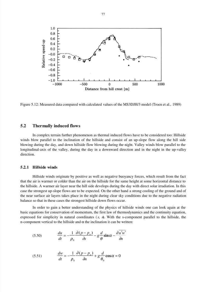
8/2/2019 Dobesch Rpt
http://slidepdf.com/reader/full/dobesch-rpt 83/123
77
Figure 5.12: Measured data compared with calculated values of the MS3DJH/3 model (Troen et al., 1989)
5.2 Thermally induced flows
In complex terrain further phenomenon as thermal induced flows have to be considered too: Hillside
winds blow parallel to the inclination of the hillside and consist of an up-slope flow along the hill side
blowing during the day, and down hillside flow blowing during the night. Valley winds blow parallel to the
longitudinal-axis of the valley, during the day in a downward direction and in the night in the up-valley
direction.
5.2.1 Hillside winds
Hillside winds originate by positive as well as negative buoyancy forces, which result from the fact
that the air is warmer or colder than the air on the hillside for the same height at some horizontal distance to
the hillside. A warmer air layer near the hill side develops during the day with direct solar irradiation. In this
case the strongest up-slope flows are to be expected. On the other hand a strong cooling of the ground and of
the near surface air layers takes place in the night during clear sky conditions due to the negative radiation
balance so that in these cases the strongest hillside down flows occur.
In order to gain a better understanding of the physics of hillside winds one can look again at the
basic equations for conservation of momentum, the first law of thermodynamics and the continuity equation,
expressed for simplicity in natural coordinates ( s, n). With the s-component parallel to the hillside, the
n-component vertical to the hillside and α the inclination it can be written:
(5.50)n
wud g
s
p p
dt
du a
∂
∂ α
θ ∂
∂
ρ
′′−−
−−= sin
)(
0
1
(5.51) 01
00≈+
−−= α θ ∂
∂
ρ cos)( d
g n
p p
dt
dwa
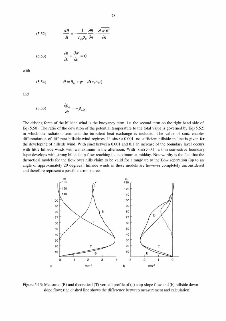
8/2/2019 Dobesch Rpt
http://slidepdf.com/reader/full/dobesch-rpt 84/123
78
(5.52)n
w
n
R
cdt
d
p ∂
θ ∂
∂
∂
ρ
θ ′′−−=
0
1
(5.53)∂
∂
∂
∂
u
s
w
n+ = 0
with
(5.54) ),,( t n sd z ++= γ θ θ 0
and
(5.55) g
z
pa
a ρ
∂
∂ −=
The driving force of the hillside wind is the buoyancy term, i.e. the second term on the right hand side of
Eq.(5.50). The ratio of the deviation of the potential temperature to the total value is governed by Eq.(5.52)
in which the radiation term and the turbulent heat exchange is included. The value of sinα enables
differentiation of different hillside wind regimes. If sinα < 0.001 no sufficient hillside incline is given for
the developing of hillside wind. With sinα between 0.001 and 0.1 an increase of the boundary layer occurs
with little hillside winds with a maximum in the afternoon. With sinα > 0.1 a thin convective boundary
layer develops with strong hillside up-flow reaching its maximum at midday. Noteworthy is the fact that the
theoretical models for the flow over hills claim to be valid for a range up to the flow separation (up to an
angle of approximately 20 degrees), hillside winds in these models are however completely unconsidered
and therefore represent a possible error source.
Figure 5.13: Measured (B) and theoretical (T) vertical profile of (a) a up-slope flow and (b) hillside down
slope flow; (the dashed line shows the difference between measurement and calculation)
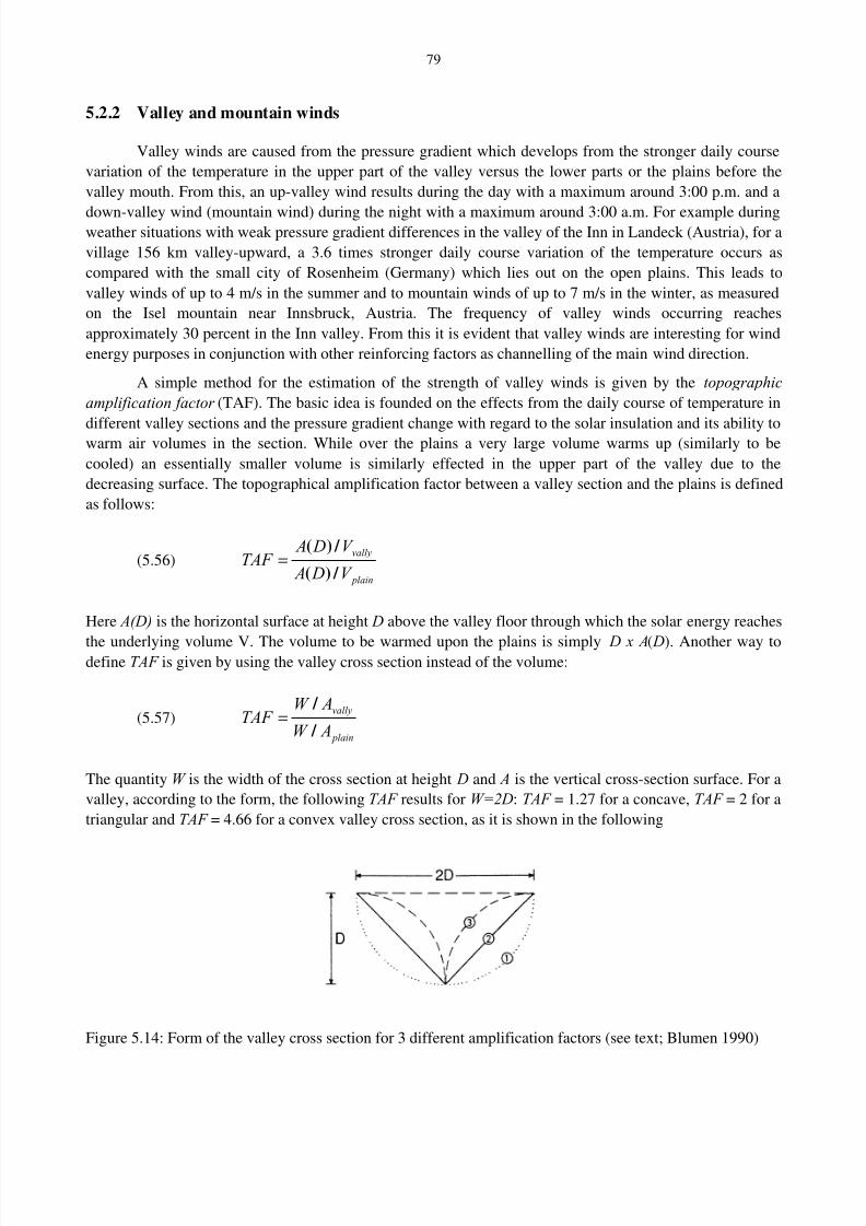
8/2/2019 Dobesch Rpt
http://slidepdf.com/reader/full/dobesch-rpt 85/123
79
5.2.2 Valley and mountain winds
Valley winds are caused from the pressure gradient which develops from the stronger daily course
variation of the temperature in the upper part of the valley versus the lower parts or the plains before the
valley mouth. From this, an up-valley wind results during the day with a maximum around 3:00 p.m. and a
down-valley wind (mountain wind) during the night with a maximum around 3:00 a.m. For example duringweather situations with weak pressure gradient differences in the valley of the Inn in Landeck (Austria), for a
village 156 km valley-upward, a 3.6 times stronger daily course variation of the temperature occurs as
compared with the small city of Rosenheim (Germany) which lies out on the open plains. This leads to
valley winds of up to 4 m/s in the summer and to mountain winds of up to 7 m/s in the winter, as measured
on the Isel mountain near Innsbruck, Austria. The frequency of valley winds occurring reaches
approximately 30 percent in the Inn valley. From this it is evident that valley winds are interesting for wind
energy purposes in conjunction with other reinforcing factors as channelling of the main wind direction.
A simple method for the estimation of the strength of valley winds is given by the topographic
amplification factor (TAF). The basic idea is founded on the effects from the daily course of temperature in
different valley sections and the pressure gradient change with regard to the solar insulation and its ability towarm air volumes in the section. While over the plains a very large volume warms up (similarly to be
cooled) an essentially smaller volume is similarly effected in the upper part of the valley due to the
decreasing surface. The topographical amplification factor between a valley section and the plains is defined
as follows:
(5.56) plain
vally
V D A
V D ATAF
/ )(
/ )(=
Here A(D) is the horizontal surface at height D above the valley floor through which the solar energy reaches
the underlying volume V. The volume to be warmed upon the plains is simply D x A( D). Another way todefine TAF is given by using the valley cross section instead of the volume:
(5.57) plain
vally
AW
AW TAF
/
/ =
The quantity W is the width of the cross section at height D and A is the vertical cross-section surface. For a
valley, according to the form, the following TAF results for W=2D: TAF = 1.27 for a concave, TAF = 2 for a
triangular and TAF = 4.66 for a convex valley cross section, as it is shown in the following
Figure 5.14: Form of the valley cross section for 3 different amplification factors (see text; Blumen 1990)

8/2/2019 Dobesch Rpt
http://slidepdf.com/reader/full/dobesch-rpt 86/123
80
However, beside the topography further factors play a role for the strength of the valley winds.
Differences in the albedo can reinforce or reduce the daily course of temperature between the plains and the
end of the valley and a stable stratified atmosphere can restrict the height D to a lower level than the
topographically pre-determined one. This leads to a greater daily course than expected from the
topographical amplification factor for convex valleys.

8/2/2019 Dobesch Rpt
http://slidepdf.com/reader/full/dobesch-rpt 87/123
81
6 MODELLING OF WIND FIELDS
6.1 Introductory remarks
A prerequisite in the siting procedure of wind power plant location of a single installation as well asfor a wind farm is the knowledge of the possible annual energy yield and also therefore the local wind field.
Only then can the information be used to verify the economic feasibility of a WEC. Furthermore, for the
assessment of optimal sites for a WEC installation within a domain, numerical flow models providing an
objective interpolation algorithms for the wind vector must be applied. As discussed in paragraph 6.6, the
frequency-distribution of the wind speed at hub-height and the height-reduced air density as well as
installation-specific parameters must be well known, such as the power curve and the technical availability.
Ideally the measurements of wind vectors should be taken at hub-height over a time period of at least two
years for statistical reasons (representativeness). In practice these measurements are rarely available as the
present common converters have hub-heights between 30 and 65 meters, and measurements at this height are
technically difficult and therefore very costly. This is why estimation by means of mathematical-physical
models on the basis of long-term time series measured by an existing meteorological network is necessary.To apply models instead of or in addition to in-situ measurements is nearly an imperative because of the
financial and temporal constraints (Dobesch et al., 1996).
It would not be pragmatic to give a thorough presentation of the great number of models in use here.
An extensive overview can be found in Lalas et al. (1996) chapters 6-9 and in Physicks (1988) for models
over complex terrain. So we can distinguish between different numerical model designs according to the
physical principles considered. These models can be roughly divided into two general categories, namely in
diagnostic (or kinematic) models and prognostic (or predictive, dynamic, primitive equations) models.
Diagnostic models take an initial set of observations scattered over a domain and try to reproduce a complete
flow field over the whole period of observations, satisfying some physical constraints (mostly mass
conservation). Prognostic models forecast the state of the flow field future - based on an initial state of theatmosphere and given boundary conditions. In this category the codes called JH-models (after
Jackson&Hunt, 1975) can be included too (despite the fact that they are neglecting their time-dependence).
But Troen claims in Lalas et al. (1996) that the JH models are to be preferred to the mass-consistent method.
We will keep with this opinion in the following.
The solution of the full set of equations in the prognostic models is still a laborious task and the
more elaborate the model is, the more reliable the input data must be to exploit the offered advantages - but
often such data are not available. Alternatively, the relative simplicity of diagnostic models makes them
attractive for many practical purposes especially as observed data from the domain of investigation can be
easily taken into consideration. Thus Pennel (1983) found that in some cases improved mass-consistent
models could outperform the more complex dynamical models.Two main types of diagnostic models can be distinguished. One type relies on the Jackson&Hunt
(1975) theory (cf. above) from which a more simplified approach can be found in Troen et al. (1986).
Typically representative models are found in Mason and Sykes (1979), Walmsley et al. (1986) and that used
in the European Wind Atlas (Troen et al., 1989). Another type is the so-called mass-consistent approach.
Here only the equation of mass conservation is used to correct an initial “guess” of the flow field (e.g. by
spatial interpolation between observed wind vectors in the domain under consideration for the given
orography). Representations of these models are the NOABL (Traci et al., 1977, 1978; Phillips, 1979) and
many variants as AIOLOS (Tombru et al., 1990) and its latest version WINDS (Ratto et al., 1990) ,
COMPLEX (Bhumrakar et.al., 1980; Endlich et al., 1983) , MATHEW, ZAWINOD2 (Dobesch et al., 1999)
and others.From a more practical point of view roughly three categories of calculation procedures can be
identified:
8/2/2019 Dobesch Rpt
http://slidepdf.com/reader/full/dobesch-rpt 88/123
82
The first group includes simple one-dimensional calculation procedure for the vertical extrapolation
of the wind speed to hub-height from measured data at lower levels (mostly 10 meters above ground level),
based on the conditions for plain terrain and therefore usually the logarithmic wind profile is applied and,
eventually, the stability of the atmosphere or changes in surface roughness are taken into account. The
application of these procedures is restricted however to plain surfaces. Typical of this group are the ALWIN
procedure, developed by DEWI (German Wind Energy Institute), as well as the Danish WAsP (Troen etal.,1989) without the orography module.
The second group comprises models in which slightly inhomogenous terrain can be taken into
account, in accordance with the theory of Jackson&Hunt. Other models of this category are the BZ code
(integrated in WAsP ) and the MS3DJH/3R model family (Walmsley et al., 1986) together with the MS-
Micro/2 code - a microcomputer implementation of the MS3DJH/3R code.
The third group includes wind field models for inhomogeneous terrain, which are based either on the
fulfilment of the continuity-equation (the so-called mass-consistent models), or, additionally, on the
conservation of momentum and on a non-hydrostatic atmosphere, (the so-called non-hydrostatic models).
Mass-consistent variational-analytical models are far spread and exist in many versions e.g. in
Sherman (1978) or above mentioned ZAWIMOD2 with a variation-analytical base. Representative of thenon-hydrostatic models is the GESIMA model (Mengelkamp, 1991) from the German Research-Centre
Geesthacht. It should be mentioned that for single points in the calculation procedures of the first and second
group by repeated application, area-related information can be achieved in the case of a regionally uniform
wind field.
As examples the ZAWIMOD2 and the Danish WAsP (which forms the basis for the European Wind
Atlas) and GESIMA model are introduced in the following paragraphs.
6.2 Mass-consistent models with variational-analytical base
One can simplistically look at this model category, as an intelligent interpolation-extrapolation of
measurements in non-homogenous terrain: Wind vector measurements from the domain of investigation are
used for an estimation of the so-called initial wind field , the three-dimensional wind field for each node of
the surface grid. To fill in the gaps between and beyond the single measurement points must be extrapolated
in the vertical and horizontal directions. In the vertical direction the above mentioned logarithmic wind
profile can be applied with or without additional terms for the stability of the atmosphere or the power-law is
used. Above the height of the Prandtl-layer the wind vector can be considered in good approximation as
constant. In the horizontal direction, the estimated values for the wind vector at the grid points are obtained
in the simplest case by a weighted average of the measurements. The weights are given by the reciprocal
value of the square of the horizontal distance from the grid points to the points with measurements (Barnard,
1991; Dobesch et al., 1999).
(6.1)
= ∑ ∑
= =
→→ M
m
M
m
mmmm r r z y xv z y xv1 1
22
00 ) / 1( / ) / ),,((),,(
The quantities x, y, z are the co-ordinates of the grid point for which the interpolated wind vector is
calculated, xm , ym, z those of the grid point at the height z for the measuring station, M is the number of
stations used and r m the horizontal distance of the grid point from the station M . Because the vertical wind
speed is not available routinely, the vertical wind component is set to zero for the entire model domain.
In the next step the initial wind field is modified so that firstly, the u, v, w components fulfil thecontinuity-equation and secondly, the modification within the investigated space must be a minimum
(Sherman, 1978). These conditions are fulfilled, if
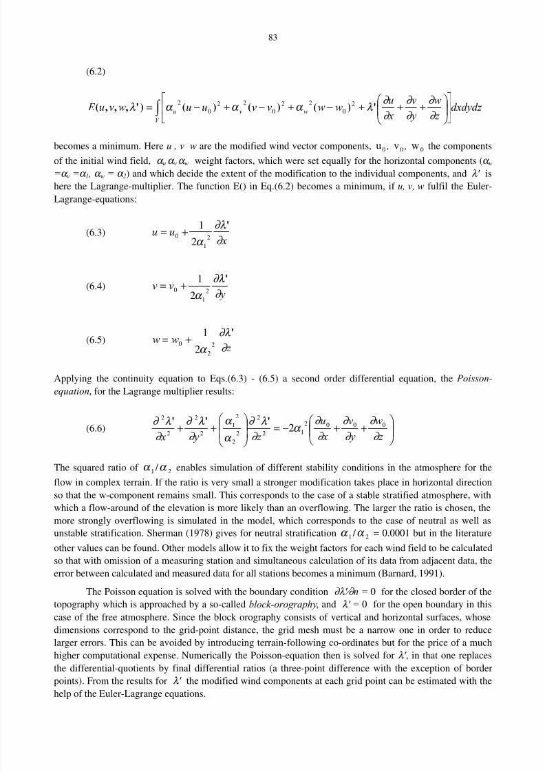
8/2/2019 Dobesch Rpt
http://slidepdf.com/reader/full/dobesch-rpt 89/123
83
(6.2)
dxdydz z
w
y
v
x
uwwvvuuwvu E
V
wvu∫
+++−+−+−=
∂
∂
∂
∂
∂
∂ λ α α α λ ')()()()',,,( 2
0
220
220
2
becomes a minimum. Here u , v w are the modified wind vector components, u0 , v0 , w 0 the components
of the initial wind field, α u α v α w weight factors, which were set equally for the horizontal components (α u=α v =α 1 , α w = α 2) and which decide the extent of the modification to the individual components, and λ ' is
here the Lagrange-multiplier. The function E() in Eq.(6.2) becomes a minimum, if u, v, w fulfil the Euler-
Lagrange-equations:
(6.3) x
uu∂
∂λ
α
'2
1
02
1+=
(6.4) y
vv∂
∂λ
α
'2
1
02
1+=
(6.5) z
ww∂
∂λ
α
'2
2
02
1+=
Applying the continuity equation to Eqs.(6.3) - (6.5) a second order differential equation, the Poisson-
equation, for the Lagrange multiplier results:
(6.6)
++−=
++
z
w
y
v
x
u
z y x ∂
∂
∂
∂
∂
∂ α
∂
λ ∂
α
α
∂
λ ∂
∂
λ ∂ 0002
12
2
2
2
2
1
2
2
2
2
2'''
The squared ratio of α 1 / α 2 enables simulation of different stability conditions in the atmosphere for the
flow in complex terrain. If the ratio is very small a stronger modification takes place in horizontal direction
so that the w-component remains small. This corresponds to the case of a stable stratified atmosphere, with
which a flow-around of the elevation is more likely than an overflowing. The larger the ratio is chosen, the
more strongly overflowing is simulated in the model, which corresponds to the case of neutral as well as
unstable stratification. Sherman (1978) gives for neutral stratification α 1 / α 2 = 0.0001 but in the literature
other values can be found. Other models allow it to fix the weight factors for each wind field to be calculated
so that with omission of a measuring station and simultaneous calculation of its data from adjacent data, the
error between calculated and measured data for all stations becomes a minimum (Barnard, 1991).
The Poisson equation is solved with the boundary condition ∂λ ' ⁄∂ n = 0 for the closed border of the
topography which is approached by a so-called block-orography, and λ ' = 0 for the open boundary in this
case of the free atmosphere. Since the block orography consists of vertical and horizontal surfaces, whose
dimensions correspond to the grid-point distance, the grid mesh must be a narrow one in order to reduce
larger errors. This can be avoided by introducing terrain-following co-ordinates but for the price of a much
higher computational expense. Numerically the Poisson-equation then is solved for λ ' , in that one replaces
the differential-quotients by final differential ratios (a three-point difference with the exception of border
points). From the results for λ ' the modified wind components at each grid point can be estimated with the
help of the Euler-Lagrange equations.
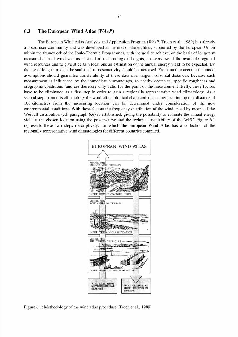
8/2/2019 Dobesch Rpt
http://slidepdf.com/reader/full/dobesch-rpt 90/123
84
6.3 The European Wind Atlas (WAsP)
The European Wind Atlas Analysis and Application Program (WAsP , Troen et al., 1989) has already
a broad user community and was developed at the end of the eighties, supported by the European Union
within the framework of the Joule-Thermie Programmes, with the goal to achieve, on the basis of long-term
measured data of wind vectors at standard meteorological heights, an overview of the available regionalwind resources and to give at certain locations an estimation of the annual energy yield to be expected. By
the use of long-term data the statistical representativity should be increased. From another account the model
assumptions should guarantee transferability of these data over larger horizontal distances. Because each
measurement is influenced by the immediate surroundings, as nearby obstacles, specific roughness and
orographic conditions (and are therefore only valid for the point of the measurement itself), these factors
have to be eliminated as a first step in order to gain a regionally representative wind climatology. As a
second step, from this climatology the wind-climatological characteristics at any location up to a distance of
100 kilometres from the measuring location can be determined under consideration of the new
environmental conditions. With these factors the frequency-distribution of the wind speed by means of the
Weibull-distribution (c.f. paragraph 6.6) is established, giving the possibility to estimate the annual energy
yield at the chosen location using the power-curve and the technical availability of the WEC. Figure 6.1
represents these two steps descriptively, for which the European Wind Atlas has a collection of the
regionally representative wind climatologies for different countries compiled.
Figure 6.1: Methodology of the wind atlas procedure (Troen et al., 1989)
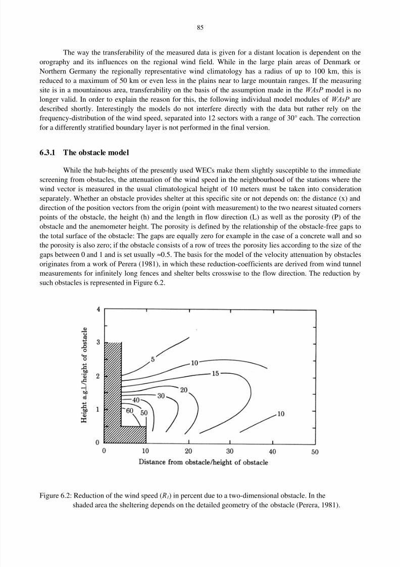
8/2/2019 Dobesch Rpt
http://slidepdf.com/reader/full/dobesch-rpt 91/123
85
The way the transferability of the measured data is given for a distant location is dependent on the
orography and its influences on the regional wind field. While in the large plain areas of Denmark or
Northern Germany the regionally representative wind climatology has a radius of up to 100 km, this is
reduced to a maximum of 50 km or even less in the plains near to large mountain ranges. If the measuring
site is in a mountainous area, transferability on the basis of the assumption made in the WAsP model is no
longer valid. In order to explain the reason for this, the following individual model modules of WAsP aredescribed shortly. Interestingly the models do not interfere directly with the data but rather rely on the
frequency-distribution of the wind speed, separated into 12 sectors with a range of 30° each. The correction
for a differently stratified boundary layer is not performed in the final version.
6.3.1 The obstacle model
While the hub-heights of the presently used WECs make them slightly susceptible to the immediate
screening from obstacles, the attenuation of the wind speed in the neighbourhood of the stations where the
wind vector is measured in the usual climatological height of 10 meters must be taken into consideration
separately. Whether an obstacle provides shelter at this specific site or not depends on: the distance (x) anddirection of the position vectors from the origin (point with measurement) to the two nearest situated corners
points of the obstacle, the height (h) and the length in flow direction (L) as well as the porosity (P) of the
obstacle and the anemometer height. The porosity is defined by the relationship of the obstacle-free gaps to
the total surface of the obstacle: The gaps are equally zero for example in the case of a concrete wall and so
the porosity is also zero; if the obstacle consists of a row of trees the porosity lies according to the size of the
gaps between 0 and 1 and is set usually ≈0.5. The basis for the model of the velocity attenuation by obstacles
originates from a work of Perera (1981), in which these reduction-coefficients are derived from wind tunnel
measurements for infinitely long fences and shelter belts crosswise to the flow direction. The reduction by
such obstacles is represented in Figure 6.2.
Figure 6.2: Reduction of the wind speed ( R1) in percent due to a two-dimensional obstacle. In theshaded area the sheltering depends on the detailed geometry of the obstacle (Perera, 1981).
8/2/2019 Dobesch Rpt
http://slidepdf.com/reader/full/dobesch-rpt 92/123
86
The effect of porosity P (with 0 ≤ P ≤ 1) is approximately accounted for by multiplication with (1–P ). If
beside the porosity P also the lateral dimension of the obstacle is regarded by a factor R2 the corrected
speed corr u with the reduction-coefficients R1 and R2 is
(6.7) [ ])( P R Ruucorr −⋅−= 11 12
The quantity R2 has to be introduced because the shelter from an obstacle with a finite lateral dimension
decreases due to mixing in the wake. Furthermore the effect in the average wind speed in a given azimuth
sector is decreased too because of the finite angular dimension of the obstacle as seen from the site.
Therefore in a given sector the reduction in average wind speed is, derived from simple geometrical
considerations,
( 1 + 0.2 x/L)-1 for L/x ≥ 0.3
(6.7.1) R2 =
2 L/x for L/x ≤ 0.3
6.3.2 The roughness model
The logarithmic wind profile can be applied only if the upwind terrain is reasonable homogeneous.
But an unique roughness-length is only available in the rarest cases. However, it is possible for small-scale
terrain inhomogenities to model the change of surface stress which occurs when flows are crossing a change
in surface roughness. In this case an internal boundary layer grows downwind from the change. Considering
a point at a distance x (the fetch) downwind of this change the internal boundary layer has grown to a height
h (Panofsky 1973), similar to Eq.(4.72).
(6.8) ′=−′′
0
0
0
901 z
x z h
z
h.]) / [ln(
where z 0' is the bigger of the upwind ( z o1) and the down wind ( z o2) roughness length. It can be empirically
found that the change of the friction velocity is well modelled using the relation
(6.8.1) u*2 /u*1 = ln(h/z o1) / ln(h/z o2)
With the knowledge of the height h the vertical profile can be considered as a profile composed from
three logarithmic parts where the lowermost part reaches approximately one tenth, the middle part up to one
third of the internal boundary layer height. However, this approach requires the restrictive condition by the
existence of several roughness changes that this one lying further away must have the double distance as that
lying closer to the measuring station (Troen et al., 1989).
6.3.3 The orographic model
The orographic model (BZ-model) of the WAsP -programme is used to correct orographically
induced disturbances in the flow field due to terrain inhomogenities. Because the BZ model is based as the
whole MS3DJH model family on the theory of Jackson&Hunt (1975) it provides only for hills with a height
up to 200 meters and a hillside inclination of up to 20 degrees for realistic results. In this geometrical range a
good approximation for the speed-up can be calculated by means of the application of polar co-ordinates and
a zooming grid.
8/2/2019 Dobesch Rpt
http://slidepdf.com/reader/full/dobesch-rpt 93/123
87
As presented already in section 5.1.4 a potential flow with the resulting flow perturbations is
determined initially. For this case it is assumed that the Laplace equation is fulfilled, if the vector field of the
wind is non-vortical, i.e. the velocity perturbation→′u (u,v,w) is related to the potential χ by
(6.9) χ ∇=′→
u
For the three-dimensional case the potential results under the assumption that the disturbance potential
vanishes at the outer boundary R (= outer model radius). A general solution can be expressed in polar co-
ordinates in terms of a sum of the products of Fourier-Bessel series with the argument c(n,j)r/R for each n
and of Fourier series with the argument exp(inϕ ) (ϕ = azimuth) with the coefficients K n,j. These coefficients
are estimated by the kinematic boundary condition on the ground (hillside-parallel flow):
(6.10) ),( ϕ ∂
∂χ r hu
z w
z
∇⋅==→
=0
0
0
where wo is the terrain-induced vertical velocity and h the height of terrain. By defining the model centre to
coincide with the point of interest it is possible to concentrate the model resolution there and also to restrict
the calculations to the perturbation at this point. For the centre point (r=0) the following solution is found:
(6.11)
−=∇
R
z c
R
c K i j
j
j j
1
1
112
1exp),( χ
In a second step the influences of friction are taken into account in the inner layer with the layer thickness l.
For the calculation of l in the BZ model, Eq.(5.36) is used but the speed-up according to Eq.(5.42) shouldlead to an overestimation of the speed amplification after Hoff (1989). However, the comparison with
measured data of the Askervein Hill shows a good agreement of theory and measurement (Troen et al.,
1989).
6.4 The GESIMA model
This non-hydrostatic model is based beside the conservation of momentum and the continuity-
equation also on the conservation of energy and the moisture balance, and uses the so-called flow-form of
terrain following co-ordinates whose vertical component is a function of the terrain height and the upper
boundary of the model space. To account also for small-scale circulation that result from dynamicallygenerated pressure differences (blocking or canalling effects), the pressure is partitioned into three parts, the
basic pressure - defined by the temperature field, the hydrostatic and the non-hydrostatic pressure deviation.
The hydrostatic part is determined from the hydrostatic basic equation and the non-hydrostatic from the
Poisson equation. The Reynolds´ shear stress is parameterised by means of the K-theory and the velocity at
the upper boundary of the model is given by the geostrophic wind.
In order to assess the average annual wind energy potential at a certain point or on a surface the two-
dimensional frequency-distribution of the geostrophic wind must be known in N speed-classes and K
directional sectors. By means of this frequency-distribution f k n, the average wind energy flow can be
determined for each place:

8/2/2019 Dobesch Rpt
http://slidepdf.com/reader/full/dobesch-rpt 94/123
88
(6.12)
322
112
1
+= ∑∑
== GEO
nn
gk
N
n
nk
K
k V
vuu f E ,ρ
gk u is the average geostrophic wind in the class k , V GEO is the amount of the geostrophic wind at the upperboundary of the model, and nu and nv are the components of the wind vector for the simulation with V GEO
from the directional sector N .
Although a great step was made with the GESIMA model in the direction for realistic representation
of wind fields in complex terrain by means of models only, a low spatial resolution is only possible now due
to the enormous computing capacities required.
6.5 Model comparison
To relate measurements of wind velocity on hills some attempts have been made to relate them totopographic features. A list of such measurements is given in Taylor et al. (1987). On the basis of such data
sets especially those from Askervein Hill, or Kettles Hill (Barnard, 1991; Bradley et al.,1989 and paragraph
5.1.4) many comparisons between different models can be found in the literature which are not easy to
follow as often modifications were made during the use and adaptations for the models to better fit to the
given conditions. A good overview is given in Walmsley et al. (1990) or Walmsley et al. in Lalas (1996)
where the results of 3 codes based on the JH theory and one mass-consistent ( NOABL) code based on a data
set from the Blashaval Hill experiment in Scotland were examined. The results show a good agreement with
each other and fell within the observed range of variation from the observations. However, gradual
differences arose from the given orography and the treatment of the roughness in the upwind fetch. In
another study Guo et al.(1990) adapted the COMPLEX and NOABL models resulting in a new model, called
MC-3. Troen states (in Lalas et al., 1996) that the mass-consistent codes fall naturally short in the treatment
of the flow physics but have advantages in the ability to incorporate directly a number of data in the analysis
and, consequently, the advantages of both model types should be linked which was achieved in the LINCOM
model (Troen, 1987, unpublished). In these studies the guidelines from the method after Walmsley et al.
(1982 and 1989) were used showing a slightly better adaptation of the model results to the given wind field.
8/2/2019 Dobesch Rpt
http://slidepdf.com/reader/full/dobesch-rpt 95/123
89
7 SITING AND ENERGY YIELD
7.1 The importance and requirements of siting
In Europe for modern WECs typical values of rated power are 600 W/m2
but for the same rated
power it can vary by 50 percent (Lalas et al., 1996). The specific energy is on average 600 KWh/m 2 /year but
with the best WECs on very good sites over 1200 KWh/m2 /year can be reached. For instance a wind speed
increase of only 1 m/s (say from 7 to 8 m/s) would result in a remarkable performance improvement so the
electricity cost drops and the capacity factor (function of technical availability - see paragraph 6.6 - and wind
resource at the specific site) would increase to 35 percent (typical 20 percent in Europe, for good sites
50 percent can be reached). This means a 20 percent increase of energy yield for a 12 percent increase in
wind speed. Therefore the importance of an accurate siting becomes paramount. Due to the fact that the wind
energy flux is proportional to the cube of wind speed, which can be written formally as
(7.1) ∫ ∝out u
uin
duuu f P 2)(
2
1ρ
(with P the energy flux and f(u) the frequency of occurrence of wind speed u; cf. paragraph 2.1) in the siting
procedure a careful identification of locations with higher wind speeds compared to other locations within a
given domain is required which is a crucial task in the exploitation of wind power.
Ideally for the estimation of energy yield for a specific WEC over its lifetime time series of wind
vector (minimum 1 year) at hub height should be available together with its mechanical and technical
availability (cf. paragraph 2.5 and 2.7). But measurements at hub height are very rare and one usually has to
rely on the data from a meteorological network in a certain standard height. Very often such data aremeasured at stations where location was usually chosen by criteria other than suitability for wind energy
issues. Therefore the data needs to be corrected before an extrapolation to hub height can be done. Both were
discussed in more detail in chapter 4 (paragraph 4.3).
7.1.1 General considerations
Wind energy systems as other energy systems have to be planned carefully to achieve reliability and
low cost. They are by their nature very sensitive to meteorological phenomena because these do not only
influence normal operation (by the given wind conditions) but can disrupt the service, augment demands or
require consideration for environmental reasons (WMO, WCAP-13).
Meteorological information for wind energy use should contain high resolution spatial maps of
regional wind climatologies derived by special algorithms. As a prerequisite, models for transforming
measured wind data into objective meso-scale representative values must be used, because measured
meteorological data very often are unrepresentative (and even of questionable quality, cf. paragraph 4.4).
Furthermore short term forecasts of wind speed (24-48 hours) for scheduling and dispatching may be a
favourable method to optimise wind energy buying and selling by the wind farm operators. These forecasts
have to be highly accurate local forecasts with an uncertainty of less than 15 percent and should be based on
a numerical weather prediction with downscaling algorithms as given in the MOS or LAM forecast products
and for a time step of at least 3 hours or less.
As a consequence the data representativeness must be given high priority. This can be achieved
through the improvement of measurements by strictly observing WMO regulations (e.g. WMO No.8, VI.6.6,
1973) without any compromises on the exposure of measuring equipment; documentation about the meta

8/2/2019 Dobesch Rpt
http://slidepdf.com/reader/full/dobesch-rpt 96/123
90
data and objective correction/reduction procedures for wind data with knowledge of shading by obstacles,
orography and environmental roughness of the site in question (cf. paragraph 6.3). Necessary additional
information and skills must be available too, e.g. DEMs (digital elevation models with a resolution of
100 x 100 meters or less), GIS tools together with land use models and remote sensed data for assessing the
areal environmental conditions of the site and representative data models such as digital databanks together
with certain geostatistical algorithms for areal interpolation of necessary parameters.
A verification of the findings can be made from ground based measurements (with a temporary or
station network), by comparison with long-term observations (from a climate network, GCOS, etc.) and by
simulation models. Fostering and improving the LAM and/or MOS analysis and forecast products can
provide the user with wind climatologies on the basis of high resolution (in time and space) data sets.
7.1.2 Meteorological data
Basically, for siting and yield estimation the following data and information must be available (with
regard to the exposure of measuring devices and representativeness of data, see above and paragraph 4.6),
defined or derived:
Measurements/observations:
Time series of wind speed and wind direction (hourly or 10-minute averages)
Maximum winds or gustiness
Lightning frequencies
Ice accretion
Meta data from station
Climatologies:
Two-dimensional probability distribution based on the time series (wind rose)
Absolute maximum of wind speed, gust and strength frequencies
Wind speed on a monthly, seasonal and yearly basis and its variations
Duration curves of expected percentage of wind speed above certain thresholds
Average air density
Two dimensional probability distribution of air humidity and air temperature (below 0° C)
Number of hours with heavy rain
Number of days with thunderstorms, lightning events and icing
Wind resource assessment usually refers to the calculation of average wind speed and its probability
distribution in different directional sectors over several years (ideally 10 - 20 years). Accurate determinationof the wind speed is of paramount importance. Additionally, special emphasis has to be put on strong and
extreme wind events and their frequency as well as on lightning strike frequency and icing conditions
because these can heavily influence power output or even the life span of WECs (cf. paragraph 3.4).
Before a specific site for the installation of a WEC can be determined a region must be found by
certain prospecting procedures where the wind speed is high. For this purpose one has to investigate the
given wind regime of a region, as far as it is unaffected by surface friction and the topographic features. This
can be done e.g. by rawinsonde measurements aloft using the geostrophic wind approach (cf. paragraph 3.2).
It is accepted that this geostrophic wind is rather constant over distances of the order of 100 km. Another
method for generalising point measurements is the exposure correction method (cf. paragraph 4.6.1) with
which a potential wind is calculated (at a blinding height ) well above local surface inhomogenities and
which is then typical for a distance of up to 50 km. For the micro-siting one can either measure the wind
vector at the site of interest (but this is expensive and time consuming); or try to extrapolate the local wind
field from other measurements in the region; or deduce it from numerical simulation on a grid. For the two
8/2/2019 Dobesch Rpt
http://slidepdf.com/reader/full/dobesch-rpt 97/123
91
last mentioned procedures a wide range of computer codes and models of different complexity and data
requirements are in use (cf. chapters 4, 5 and 6). The spectrum stretches here from simple mass-consistent
models that generate wind fields, consistent with kinematic constraints imposed by the available data and the
domain of interest, to the most developed models which solve the non-hydrostatic set of the fundamental
equations of motion in the atmospheric boundary layer including different parameterisation scales for
turbulence.
7.1.3 Some aspects of predicting the wind resource on land and offshore
As in the forgoing chapter described, for wind farm development, it is essential to have a good
estimate of wind speeds from the proposed site. On land, this can be achieved in a relatively straightforward
manner by e.g. installing a mast and measuring wind speeds for a period of around a year. Then, by
statistical comparison of the long record from a nearby anemometer station maintained of a meteorological
measuring network, an evaluation of the long-term potential can be carried out (Woods et al. 1997).
Monitoring wind speeds offshore as part of the site evaluation is generally not feasible, simply
because of the cost of mast installation and monitoring. however, in the far offshore (away from the effects
of land), wind speeds vary much less in space than is the case onshore. This makes modelling wind speeds a
more straightforward exercise. Possible approaches include using reanalysis data from the National Centres
for Environmental Prediction (NCEP, Kalnay et al., 1996; see http://wesley.wwb.noaa.gov/reanalysis.html).
These gridded data go back to 1948 at a daily (or better) resolution and are continually up-dated. The grid
resolution is around 210 km. Horizontal winds are a model output, and could be used directly to estimate
wind speed. However, it is generally considered that the models used to generate the NCEP reanalysis data
simulate sea level pressure more accurately than horizontal wind speeds. Sea level pressure data can be used
to calculate the geostrophic wind speed. Then, using a boundary layer model such as WAsP (described in
Section 6.3), hub-height wind speeds can be calculated from the geostrophic winds.
Close to land, the wind field over the sea becomes much more complex due to the thermal anddynamic effects of the land on the overlying air. At the same time, it is likely for some time to come that
offshore wind farm construction will concentrate in the near-shore zone, because installation and
maintenance costs will be lower than in the far offshore. Modelling winds in the near-shore zone is not
straightforward. A number of empirical and theoretical formulae have been developed to model the
development of internal boundary layers at the coastal discontinuity (cf. paragraph 4.5.4), and the increase in
wind speed as air moves away from the land. These formulae, and methods for evaluating wind speeds in the
near offshore, are reviewed by Barthelmie et al. (1996).
7.2 Estimation of energy yield
If reliable wind measurements are available at a particular site and the procedures accounting for
different surface roughness in certain wind direction sectors at the measuring sites are applied, as described
in paragraph 4.4, the energy yield of a WEC in the time period dt results from the product of power and the
time interval:
(7.2) dt t P dE )(=
Integration over time T (e.g. 1 year) gives:
(7.3) ∫ =T
T dt t P E 0
)(
8/2/2019 Dobesch Rpt
http://slidepdf.com/reader/full/dobesch-rpt 98/123
92
After Eq.(7.3) and Eq.(2.4) one obtains
(7.4) )()()(2
1)( 3
t ut t c F t P pr ρ =
with c pr (t ) the actual over-all efficiency of the WEC for the time t and F the area of the rotor cycle. If the
turbine stands still or does not reach the intended performance because of icing, crosswinds or reduced air
density, crp is not identical to the power-coefficient c p from the power curve. For simplification the air
density is usually regarded as a pure function of height and the other deviations from c p during unaffected
operation are considered by means of the technical availability. The available energy then can be written as
(7.5) duu P u f T E N Arel T )()(∫ ∞
⋅⋅=0
ρ
with
(7.6) p N cu F u P 30
2
1)( ρ =
Here ρ rel is the relative density and T A the technical availability, which currently can be assumed as 0.95.
To calculate the energy yield using Eq.(7.6) as well as the power curve P N (u), the likelihood-density-
function f (u) must be known. It can be estimated by adaptation to the measured frequency-distribution of
the wind speed with two parametric Weibull-distribution, which belongs to the Gamma-distribution family.
The mathematical form of this distribution is:
(7.7)
−
=
− k k
A
u
A
u
A
k u f exp)(
1
The two Weibull parameters are usually named scale parameter A and shape parameter k . The dependence
of f(u) on different values of the shape parameter is illustrated in Figure 7.1. For k > 1 the maximum of f(u)
lies at values u > 0, while for 0 < k <1 it decreases monotonically. The Weibull-distribution can be reduced
to two other theoretical distribution, namely with k = 1 the exponential-distribution and with k = 2 the
Rayleigh-distribution which is sometimes used to describe wind data as for the multitude of German and
Danish sites, and therefore it is often used by WEC manufacturers for the estimation of the energy yield.
However, for non-homogenous terrain the values of the form parameter lie between 1.3 < k < 1.8, whichresults in a greater energy yield in comparison to the Rayleigh-distribution of the same average value.
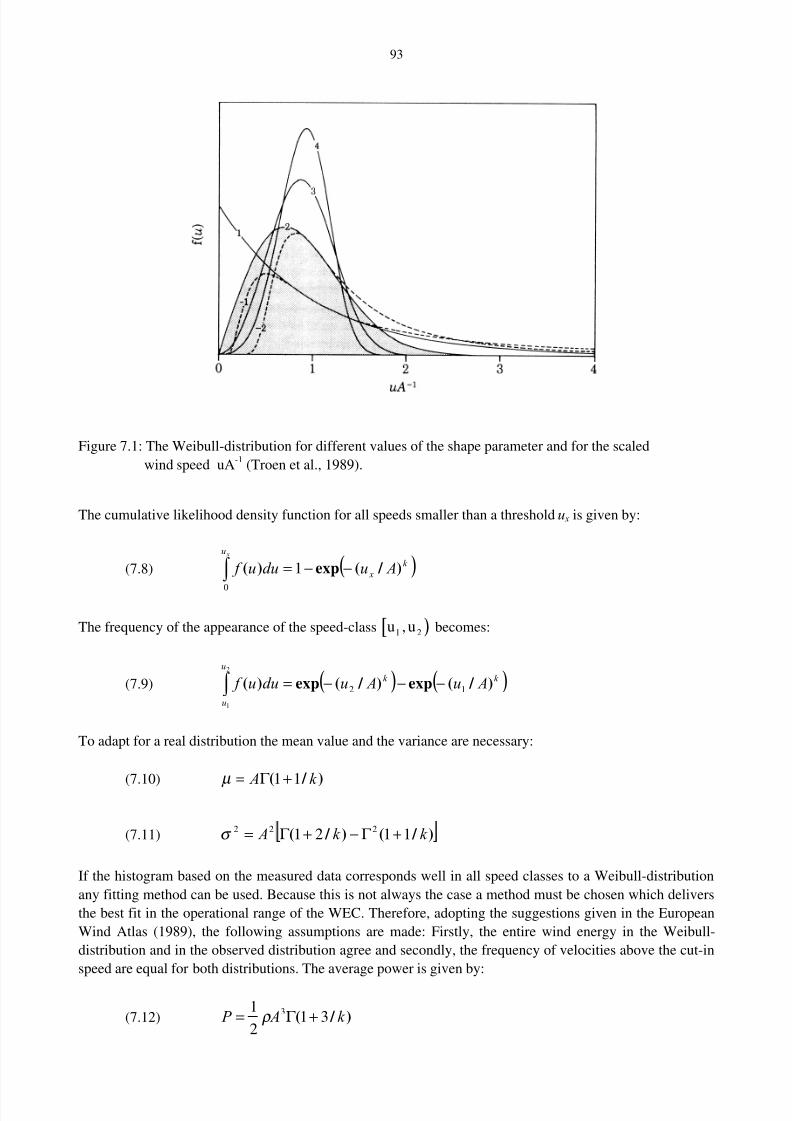
8/2/2019 Dobesch Rpt
http://slidepdf.com/reader/full/dobesch-rpt 99/123
93
Figure 7.1: The Weibull-distribution for different values of the shape parameter and for the scaled
wind speed uA-1
(Troen et al., 1989).
The cumulative likelihood density function for all speeds smaller than a threshold u x is given by:
(7.8) ( )k
x
u
Auduu f x
) / (exp)( −−=∫ 1
0
The frequency of the appearance of the speed-class [ )u u1 2, becomes:
(7.9) ( ) ( )k k
u
u
Au Auduu f ) / (exp) / (exp)( 12
2
1
−−−=∫
To adapt for a real distribution the mean value and the variance are necessary:
(7.10) ) / ( k A 11+Γ =µ
(7.11) ) / () / ( k k A 1121 222 +Γ −+Γ =σ
If the histogram based on the measured data corresponds well in all speed classes to a Weibull-distribution
any fitting method can be used. Because this is not always the case a method must be chosen which delivers
the best fit in the operational range of the WEC. Therefore, adopting the suggestions given in the European
Wind Atlas (1989), the following assumptions are made: Firstly, the entire wind energy in the Weibull-
distribution and in the observed distribution agree and secondly, the frequency of velocities above the cut-in
speed are equal for both distributions. The average power is given by:
(7.12) ) / ( k A P 312
1 3 +Γ = ρ
8/2/2019 Dobesch Rpt
http://slidepdf.com/reader/full/dobesch-rpt 100/123
94
If the wind climate of a site is known the velocity at which the WEC reaches its highest efficiency as well as
the distribution of the highest power density should preferably by in proximity. The highest efficiency
should be reached at
(7.13)
k
opt k
k Au
/ 1
2
+=
In general opt u lies between 1.4 and 2 times the value of the average wind speed. It should be mentioned
here that often a wind distribution cannot be adequately represented by a Weibull distribution. In particular,
when the wind climate has a large proportion of thermally generated winds. In such a case the best
approximation may be the sum of 2 Weibull distributions, one representing the synoptic content and the
other the thermal.
7.3 Verification
To verify the forecast of an energy yield at a certain site is an important but complicate task as the
yield data are mostly available (if ever) for a relative short period in comparison with the measurement
period from which the forecast was derived. Additionally, they are strongly dependent which basic station
and measurements were used (if no site-specific measurements have been available) relative to the site where
the WEC was eventually erected. An example in the following table (from Gerdes et al., 2000) shows this
clearly and the importance of areal interpolation procedures
Table 7.1. Energy yield forecast with respect to measurements at different locations for Northern Germany
in comparison with the measurement at a 130 meter mast; (*) from Eelde, Bremen, Helgoland
Station Bremen Eelde Helgoland 130-m mast interpolated (*)
Period 1970-1978 1970-1978 1971-1980 1993-1997
Energy yield 797 1.067 1.051 947 881 MWh/a
Forecast/actual yield 87 116 114 103 96 %
As a further example an examination of the accuracy of the WAsP model is given here that is
described thoroughly in Penner (2000). Several error sources were identified, especially for the evaluation of
the site. Three of these error sources are meteorological and one from manufacture. Possible meteorological
errors are the selection of the right basic station (because from this station the wind climatology is derived),an erroneous roughness length and the change of roughness elements in the upwind direction. This can lead
to errors of up to 35 percent in the estimation of energy yield. How far this is dependent on the roughness
length is shown in Figure 7.2. Errors in roughness length up to 25 percent result only in small errors of the
energy yield, but with larger deviations from the actual roughness theses errors increase rapidly, that shows
clearly the necessity for an objective evaluation of roughness. A variation in the horizontal distance of
roughness changes of 5 percent creates a small deviation in energy yield (0.3 percent). A frequent error
which is of concern to the manufacturer, is the specification of the power curve based on theoretical
calculations instead of measurements which leads to an overestimation of the energy yield.

8/2/2019 Dobesch Rpt
http://slidepdf.com/reader/full/dobesch-rpt 101/123
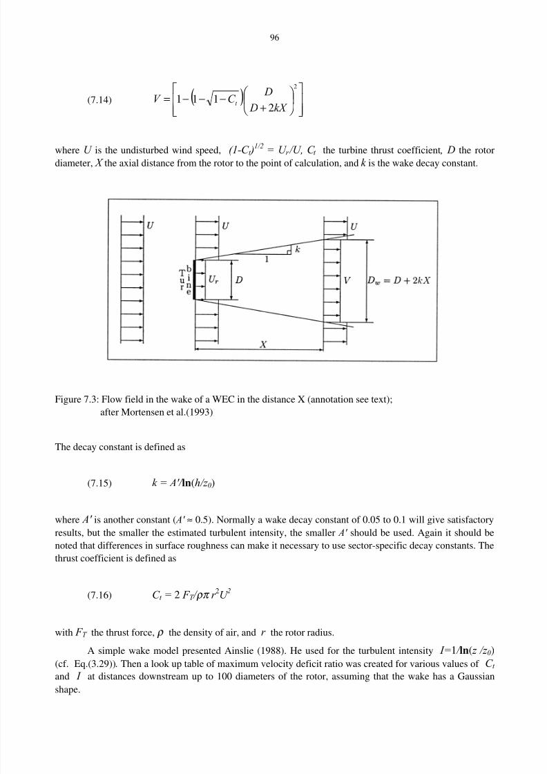
8/2/2019 Dobesch Rpt
http://slidepdf.com/reader/full/dobesch-rpt 102/123
96
(7.14) ( )
+−−−=
2
2111
kX D
DC V t
where U is the undisturbed wind speed, (1-C t )1/2
= U r /U, C t the turbine thrust coefficient , D the rotor
diameter, X the axial distance from the rotor to the point of calculation, and k is the wake decay constant.
Figure 7.3: Flow field in the wake of a WEC in the distance X (annotation see text);
after Mortensen et al.(1993)
The decay constant is defined as
(7.15) k = A'/ ln(h/z 0)
where A' is another constant ( A' ≈ 0.5). Normally a wake decay constant of 0.05 to 0.1 will give satisfactory
results, but the smaller the estimated turbulent intensity, the smaller A' should be used. Again it should be
noted that differences in surface roughness can make it necessary to use sector-specific decay constants. Thethrust coefficient is defined as
(7.16) C t = 2 F T / ρπ r 2U
2
with F T the thrust force, ρ the density of air, and r the rotor radius.
A simple wake model presented Ainslie (1988). He used for the turbulent intensity I=1 / ln( z /z 0)
(cf. Eq.(3.29)). Then a look up table of maximum velocity deficit ratio was created for various values of C t
and I at distances downstream up to 100 diameters of the rotor, assuming that the wake has a Gaussianshape.
8/2/2019 Dobesch Rpt
http://slidepdf.com/reader/full/dobesch-rpt 103/123
97
Frandsen et al.(1996) gave on the basis of the power-law relationship a velocity deficit
(7.17) δ u = 0.176 C t 0.83 / ( I 0.63 xd
0.77 )
with xd the distance downstream of the rotor plane in diameters. The added turbulence (taken as constant
over full wake width) due to the wake of upstream turbines can be calculated after Hassan et al.(1991) with
(7.18) δ I = 1.31 C t 0.71
I 0.68
( x/xn)-0.96
where x is the distance downstream of the rotor plane and xn is the near wake length. In Frandsen et
al.(1996) a similar estimation of the added turbulence is given as
(7.19) δ I = [1.2 C t xd -2]0.5
Several methods for the effect of multiple wakes on a turbine can be used. The resultant wake
velocity deficits are in the case of
Square root of the sum of squares of δ u (1-ui /U )2 = Σ(1-uij /u j)2
Energy balance U 2 - ui = Σ(u j
2- uij
2)
Geometric superposition ui /U = π uij / u j
Linear Superposition (1- ui /U ) = Σ(1- uij /u j);
where U is the wind speed, ui the velocity at the i-th turbine, uij the velocity at the i-th turbine due to the
wake of the j-th turbine. The summations are over the j turbines upstream of the i-th turbine. Some specific
tests to examine these wake combination methods have been performed by a series of wind tunnel
experiments by Hassan et al.(1990) and Smith (1990).
The aerodynamic power reduction caused by the reciprocal shading if the WECs is usually (Hau,
1996) expressed in terms of the “aerodynamic field efficiency (AFE)”. It is defined as the ration of the power
output of the whole wind farm to the sum of undisturbed power out put of all the single WECs comprising
the wind farm. In a real wind farm there is always AFE < 1, its value dependent beside on the technical
properties of the WECs themselves, on the field geometric of the wind farm (number of WECs and landarea), the turbulence intensity and the probability distribution of wind direction. The turbulence intensity is
important insofar that the loss of momentum in the wake of a WEC is filled up after a certain distance by
momentum transport from the flow in the surrounding and this is strongly dependent on the turbulence
intensity. This means the higher the turbulence intensity is the more rapidly the momentum loss is filled up
again. The turbulence intensity of the real atmosphere usually lies between 10 to 15 percent above land and
around 5 percent above the sea. This effect is enhanced in a wind farm by the rotation of the rotors. This
shows the necessity of having a good estimation about the turbulence conditions in the area. A wind farm
has a somewhat different power characteristic too: after reaching the cut-in-speed the plants in the first row
will start up, then followed by the next row and so on. From a certain flow velocity which lies above the
rated velocity specified for a single WEC within the wind farm, all WECs will operate with rated power. In
this case the field efficiency of the farm is 100 percent. Because the aerodynamic rotor drag is equivalent tothe momentum loss in the wake, it is a measure for the dimension of the wake area. Therefore rotors with
8/2/2019 Dobesch Rpt
http://slidepdf.com/reader/full/dobesch-rpt 104/123
98
high aerodynamic drag, as e.g. stall regulated ones, are disadvantageous compared with rotors with a high tip
speed ratio.
The optimal geometry of the grid of a wind farm is dependent on the field geometry and the given
grid connection. The electrical losses are a direct consequence of the grid design (voltage level, length and
cross section of cables, numbers of transformers, etc.). For large wind farms the electrical loss until the grid
should be not more than 5 percent and can be significantly lower if the output of the WECs is on a higher
voltage level (e.g. 20 kV).
7.4.2 Experiences with wind farms (on- and offshore)
The power output of a single WEC, even for the “big” ones with 2-3 MW, is low compared with a
conventional power plant. The decentralized arrangement of WECs in densely populated areas reaches
quickly its limits. Additionally, areas with technical usable wind energy potentials are in most countries
limited to certain regions. On account of this there is a need to concentrate a larger number of WECs in these
regions independently of their own energy demand. Beside this the spatial concentration of WEC has many
technical advantages for construction, operation and maintenance of such wind farms. Many experts believe
therefore that under commercial conditions a minimum of 10 to 20 WECs are necessary. Due to the need of
space of such wind farms agricultural areas can be used ideally in countries where only limited space is
available as it is mostly the case in Europe. An alternative are off-shore wind farms.
But not only areas with a good wind potential are favorable for wind farms, (governmental)
subsidies or offered tax credits or paying for the “green energy” on the scheme of “maximum avoided costs”
were also necessary in the past (and today) to promote wind energy as it was the case in the U.S.A. (PURPA,
cf. chapter 1.4). In Europe one of the first wind farm was constructed near Tandpipe in Jütland, Denmark. In
Great Britain the begin of extensive use of wind energy was started by the “Non Fossil Obligation Program”
(NFFO) between 1990 and 1994. Large wind farms can be found too in Spain (e.g. near Tarifa) and Portugal.
But now in may part of the world wind farms are under operation and planned as in India and in China.Especially here great attempts were made in the last few years. So e.g. the Huitengxile wind farm in Inner
Mongolia will be pushed from 5 MW in 1995 to 200 MW in 2005 and even to 600 MW in 2010.
With offshore wind farms experiences are quite short because there are until now only a few
working operationally. One of the fist (actually the forth worldwide) was the Swedish Bockstigen farm
(Lang et al., 1999), West off the coast of Gotland island, operating since March 1998. This farm resulted
from a demonstration in the EU-THERMIE program framework and can stand as a model for many other
offshore wind farms to be constructed. This wind farm consists of five 550 kW turbines which were
especially adapted for the offshore conditions. The speed control system was optimized so it performs two
main functions: Firstly, at low wind speeds (up to 20% of rated power output) the WEC operates as
frequency converter. The turbines generators run with variable speed to increase the power output. Secondly,At medium or high wind speeds the WECs are directly grid coupled where the power converter operates as a
precision blind current source. The lessons learned from this farm are that wind, wave and sea current
conditions at the site have to be carefully investigated as well as the given conditions for the anchoring of the
sea cables and the monopile foundation. Additionally, measurements were performed at the Bockstigen
turbines as well as at turbines of identical type of land for direct comparison of the power output between
onshore and offshore WECs.
Beside all this technical aspects the perspectives of environmental protection have to be considered
thoroughly and with high accuracy as it has been done e.g. during the planning for the Borkum-West
offshore wind farm in Germany (Erdmann et al.2000). All possible sphere of influences on the living
environment during the construction phase and the operation were investigated and measure wererecommended where such influences were identified and a monitoring concept was developed to assess and
document the environmental impact now and in future (see following chapter 8).
8/2/2019 Dobesch Rpt
http://slidepdf.com/reader/full/dobesch-rpt 105/123
99
8 ENVIRONMENTAL IMPACT OF WECS
Each energy system has, in varying degrees, associated with it positive and negative impacts on the
environment. Traditional energy planning and cost/benefit analysis has ignored until now environmental
externalities (the environmental damages on air and water quality, land use, global climate and biodiversity)
but increasing efforts were made recently, leading to impact-pathway approaches, estimating e.g. the damage
from a fossil fuel plat in terms of the value of the reduced life span and well-being of persons impacted by
the plant's emissions. In 1995 a study "Externalities of Energy" ( ExternE ) sponsored by the European
Commission in the UK, made a comprehensive effort to quantify monetary values of environmental
externalities for a wide range of fuel cycles (coal, oil, gas, hydro, nuclear and wind) including the following
environmental impacts: global warming, acidification, land use, occupation and public accidents, bird
mortality, noise, visual amenity and radio interference. Though wind energy itself produces no gaseous
emissions, during its construction and installation impacts are generated. This has been quantified by the
above mentioned study for two wind farm sites in UK.
Table 8.1: Environmental externality values for wind-generated electricity and its external costs
in 1/10 Euro-Cent/kWh (ExternE, 1995)
noise global warming acidification occupational / public accidents visual amenity
0.07 - 1.1 0.15 0.7 0.26 0.09 not quantified
With these numbers wind energy's environmental impact appear no higher than any other fuel and
considerably lower than those of fossil fuels. In addition, the impacts from wind energy are local, relatively
predictable and primarily aesthetic, compared to other energy generating systems. So the environmentalbenefits of the generation of electricity by wind turbines are clearly shown in having no pollutants at all
during operation, such reducing the carbon dioxide content of the atmosphere and, additionally, reducing the
dependency on conventional fossil and nuclear fuels. In the following some of the mentioned possible
impacts such as sound emission, the visual impact and electromagnetic interference are investigated.
8.1 Sound emission from wind turbines
The aerodynamic noise produced by WECs can perhaps best be described as a 'swishing' sound
(Boyle, 1996). It is affected by the shape of the blades (especially the trailing edge and the tip shape), the
interaction of the air flow with the blades and the tower, and the turbulent wind conditions that can cause
unsteady forces on the blades which then radiate noise. Noise nuisance is usually more of a problem in light
winds because for higher winds the noise from the WECS is partially masked by the background noise.
The sound heard from a source in the landscape is strongly dependent on the distance, the height of
the source and the topographic features of the landscape itself and also on the conditions in the atmosphere
(wind speed and direction and stratification of the air mass). But for most contemporary turbines available,
sound emission is only a minor problem due to new designs of quieter rotor blade tips. The sound intensity
falls with the square of the distance from the sound source where, additionally, sound absorption or
reflection may play a role at a particular site. So typically a minimum distance of about 7 rotor diameters or
300 meters is given to the nearest neighbours. There is always some background noise in the landscape, and
at winds speeds around 4-5 m/s the noise from the leaves of trees, masts and fences etc. will gradually mask
any potential sound from WECs. Generally, very little sound is heard upwind of wind turbines which makes
it necessary to use the wind rose to chart the potential dispersion of sound in different directions. Further, the
8/2/2019 Dobesch Rpt
http://slidepdf.com/reader/full/dobesch-rpt 106/123
8/2/2019 Dobesch Rpt
http://slidepdf.com/reader/full/dobesch-rpt 107/123
101
The sound emission of e.g. m turbines in a wind farm can be calculated with Eq.(8.2) by summing the L p of
the m single turbines.
Usually the sound power level ( Lwa,ref ) is provided for a reference wind speed of 8 m/s in 10 meters
height (u10). Therefore the sensitivity of Lwa to wind speed is needed. Using u10 as reference speed in the
reference height the value of Lwa in Eq.(8.1) or Eq.(8.2) must be replaced with
(8.3) L' wa = m (u10 - 8) + Lwa,ref
where m is the slope of d(Lwa) /d(u10 ).
8.2 Shadow casting from wind turbines
The visual perception of a WEC is determined by a variety of factors, including turbine size anddesign, number of blades, layout of the wind farm etc. One specific factor is the flickering effect. When the
sun is visible WECs will cast a shadow on the neighbouring areas and the rotor blades chop the sunlight,
causing a flickering (blinking) effect while the rotor is in motion. This may be quite annoying for people.
Therefore the potential flicker effect has to be estimated and upon this the turbines placed where this effect is
bearable for the neighbours. Shadow casting is generally not regulated explicitly by planning authorities. But
in Germany there has been a court case in which it was decided to tolerate 30 hours of actual shadow flicker
per year on a certain neighbouring area.
This shadow flicker effect can be predicted quite accurately using astronomy and trigonometry
producing either a likely, or a "worst case" scenario, i.e. a situation where there is always sunshine, when the
wind is blowing all the time, and when the wind and the turbine rotor keep tracking the sun by yawing the
turbine exactly as the sun passes.
8.2.1 Basic considerations
The disturbing effect of the shadow cast by WECs for residents originates mainly from the shadow
of the rotor blades, rotating with a speed less than 100 U/min. The narrow, slowly moving shadow of the
tower corresponds to the shadow of high buildings and is normally not felt as disturbing. These effects
definitely originate from three factors:
• the difference of the radiation-intensity between shadow-minimum and –maximum; this is defined by
the technical parameters of the height and the rotor blade's cord length of the WEC, by the astronomicparameter of sun elevation angle and the geometrical situation between observers, the WEC and the sun;
• the temporal course of the intensity change, which is governed by the speed of rotation of the rotor and
the geometrical situation of observers, the WEC and the sun;
• the daily/yearly duration of the shadow casting resulting from the first factor under additional
consideration of the climatological values for the location.
For the human eye the allowable difference between shadow-minimum and -maximum of a wind
turbine is given here after DEWI (1998). A lower limit for the sun elevation angle is quoted as 3°: In the
atmosphere an attenuation of the direct solar radiation occurs by scattering and absorption through the air
particles (Dirmhirn, 1964). This attenuation increases exponentially with the penetrated air-mass as well as
with decreasing sun elevation (see Table 8.3). So the attenuation of the intensity with an angle of 3° at
200 meters a.s.l. amounts to approximately 80 percent of the radiation with a sun elevation of 41.8°
( standard value). With increasing height the attenuation decreases and at a height of 1000 meters a.s.l. the
8/2/2019 Dobesch Rpt
http://slidepdf.com/reader/full/dobesch-rpt 108/123
102
attenuation (with 3° of elevation angle) is only 68 percent of the standard value (see Table 8.4). As a
consequence of this, a diminution of the minimal sun elevation angle can be assumed with respect to the
height a.s.l. of about 0.5° per 500 meters.
Table 8.3: Penetrated air-mass with respect to the sun elevation (at sea level)
Sun elevation 90 70 60 50 40 30 20 15 10 5 3 (°)
True air-mass 1.0 1.06 1.15 1.3 1.55 2.0 2.9 3.8 5.6 10.4 15.4
Table 8.4: Dependency of the penetrated air-mass on the height above sea level.
Height 0 900 1900 2900 4000 5400 (m)
True air-mass 1.0 0.9 0.8 0.7 0.6 0.5
The attenuation of the radiation intensity is additionally influenced by the water vapour and dust content of
the atmosphere.
For typical construction heights the distance between the WEC and the observer is more than
1000 meters for the quoted height angles. With these distance however no kernel-shadow occurs
(100 percent masking of the sun disk by the rotor blades).
At a further low threshold, a masking of the sun disk by 20 percent is observed at the rotor blades.
This value depends on the rotor blade cord length of a specific WEC and leads to intensity differences
between 0 and approximately 20 percent. No intensity difference exists, if the focus of the rotor circle and
the sun disk are in a line. By the superimposition of the two, the intensity attenuating effects and the entireintensity difference amounts to less than 10 percent.
Regarding the temporal course of the intensity change, at present no investigations have taken place.
In all present standards, no differentiation is made where a kernel shadow or a diffuse shadow is
found. It is essential that consideration be given however, for example, a residence that lies 200 to
250 meters to the north of an installation experiences 30 hours extreme kernel-shadows (high sun elevation)
per year, or when positioned 700 to 750 meters south east of an installation when subject only to a diffuse
shadow with less than 10 percent intensity change (low sun elevation, low masking). It is possible therefore
that standard values be set up with regard to the sun elevation and the share of the masked sun disk. So it
appears realistic to reduce the possible annual shadow duration hours to zero if more than 80 percent
masking of the sun disk through the rotor blades occurs, and to increase this duration in five-hour steps to
30 hours per year with 20 percent masking. Additionally, the greatest allowable elevation angle of 15° could
be accepted as a guideline with a masking of more than 40 percent. With this elevation angle, the attenuation
reaches at 200 meters only 40 percent of the standard value. Summarising the effects of sun elevation and
masking, the intensity difference for 80 percent masking and 15° amounts to approximately 50 percent of the
value at 41.8° and 100 percent masking.
8/2/2019 Dobesch Rpt
http://slidepdf.com/reader/full/dobesch-rpt 109/123
103
Table 8.5: Recommendation for a guideline of the maximum annual shading duration (in hours)
Masking 80% 70% 60% 50% 40% 30% 20% 10%
0° to 3° - - - - - - - - -
3° to 15° 0 5 10 15 20 25 30 -
> 15° 0 0 0 0 5 10 15 -
8.2.2 Geometrical data of WECs
The construction height determines the shadow casting and therefore this height has to be considered
especially because of the considerable heights of future WECs that will rise between 85 and 100 meters.
The rotor blade depth determines the percent share of the masked sun disk within a pre-determined
distance. The rotor blade is broadest at the root and narrowest at the blade tips, the average rotor blade depth
reaches approximately 70 to 80 percent of the rotor blade depth at the root. The average rotor blade depthshould be taken for the calculation of the masking, since travel across the sun disk is more likely with the
outer part of the rotor blade due to the comparatively greater length. These data can be found in the
published information of the rotor blade manufacturers.
If no exact data are available for the rotor blade, the average rotor blade depth can be appraised using
the following formula:
Rotor blade depth (m) = 0.0306 times diameter (m) – 0.0377
The rotation speed effect decreases for technical reasons (the acoustic power level increases to the 5th
power of the blade tip speed) with greater diameter. For example WECs with three rotor blades and 30 meterdiameter have a rotation speed of approximately 40 r/min and WECs with more than 60 meter diameter
rotors have approximately 18 – 20 r/min. Two bladed installations with a rotor-diameter of 30 meter reach
rotation speeds of approximately 70 r/min. The frequency of shadow casting is 2 Hz comparable to a three
wing installation of the same size.
8.2.3 Distances for the shadow casting
The decisive distances on the basis of the construction height of the WEC and the sun elevation
angle on plain surfaces can be calculated from the geometry of the ray path. The increase of the distance
takes place linearly in dependency on the construction height and for height angles of 2°, 2.5°, 3° and 15° asshown in the following table:
Table 8.6: Influence distance in meters (m) for different height angles and construction heights
Elevation Height 50 60 70 80 90 100 110 120 m
2° 1432 1718 2005 2291 2577 2864 3150 3436 m
2.5° 1145 1374 1603 1832 2061 2290 2519 2748
3° 954 1145 1336 1526 1717 1908 2099 2290
15° 187 224 261 299 336 373 411 448

8/2/2019 Dobesch Rpt
http://slidepdf.com/reader/full/dobesch-rpt 110/123
104
The influence distance of any construction height can be calculated by means of the following formulas:
Sea level height ≥ 1000 m (height angle 2°): E = 28.636 * B
Sea level height ≥ 500 m (height angle 2.5°): E = 22.904 * B
Sea level height < 500 m (height angle 3°): E = 19.081 * B
Minimal spacing (height angle 15°): E = 3.732 * B
E = influence distance; B = construction height
The stated elevation angles of the sun and the respective distances can only be reached at 48.2° degrees of
latitude in certain directional sectors however.
Clockwise from North (0°=360°) the relevant areas for shadow casting are:
0° - 24° Shadow casting for less than 3.732 construction heights distance possible
24°–108° Shadow casting with a height angle of 15° possible
50° - 124° Shadow casting with a height angle of 2-3° possible
124° - 236° No (relevant) shadow casting possible236° - 310° Shadow casting with a height angle of 2-3° possible
252° - 336° Shadow casting with a height angle of 15° possible
336° - 360° Shadow casting for less than 3.732 construction heights distance possible
8.2.4 Distances on the basis of the masking of the sun disk by the rotor blades
The distance E(d) from the WEC, for which the rotor blades yield a masking d of the sun disk can be
calculated from the distance earth-sun ES (= 149 504*103km), the shadow width S(d) and the rotor blade
depth T as follows:
(8.4) E(d) = ES * T / S(d)
The shadow width in 103 km as well as the ratio ES and S(d) for different degrees of masking can be found
in the following table:
Table 8.7: Shadow width (103km) and ratio ES/S(d) with respect to the degree of masking (%)
Masking 80 70 60 50 40 30 20
Shadow-width 956 814 685 562 445 331 220
ES/S(d) 156.4 183.7 218.3 266.0 336.0 451.7 679.6
8.3 Visual intrusion in the landscape
The visibility of turbines in the landscape may be of some problems where landscape protection and
visual amenity are valued highly in the society. To quantify this more or less subjective impressions,
different ways accounting for visibility exist. The points of visibility can be the nacelle, the blade tip or a
point on the tower. In the case of a wind farm a simple way is to count the number of turbines and which of
the mentioned points are visible from locations in the vicinity of the wind farm site. For example, the
visibility count can be made by summing up (with possible weights) if the nacelle, the tip and/or the towercan be seen. Therefore if the whole turbine is visible the count for that turbine is e.g. 3. Simply, the
maximum count for a whole wind farm using this method is 3 times the number of turbines (without
8/2/2019 Dobesch Rpt
http://slidepdf.com/reader/full/dobesch-rpt 111/123
105
weighting). If only the topography is used in the calculations, ignoring visual sheltering effects from
buildings, trees and other structures, the theoretical maximum visibility of turbines is given for a certain
point in the vicinity. Additionally, exclusion zones can be specified where beside the topography features
like forests obscure the turbine(s).
8.4 Electromagnetic interference
Sometimes a reflection of the electromagnetic radiation can occur if a WEC is positioned between
radio, television or microwave transmitter and receiver. This is due to the reflected wave interfering with the
original signal causing a distortion which is dependent on the blade material and the surface shape of the
tower. The most likely form of interference is on television viewing but this can be dealt with relatively
easily by the installation of relay transmitters or by connecting through a cable television service (Boyle
1996). Microwave links, VHF Omnidirectional Ranging (VOR) and Instrument Landing Systems (ILS) are
very susceptible to interference.
8.5 Résumé
As a summary of this chapter it can be said that technologies that use natural energy will have somelocal impacts such as visual intrusion or disruption of local ecosystems. This means that the local impactsassociated with energy technology should be minimised and any remaining local impacts should be tradedoff against the global environmental benefits of the technology. Furthermore, extracting more energy fromnatural resources than the local ecosystem can cope with must be avoided. In this matter environmentalists,climatologists and hydrologists are requested to monitor these developments through an effectiveobservation (on large scales as e.g. GCOS and local scales) and information system.

8/2/2019 Dobesch Rpt
http://slidepdf.com/reader/full/dobesch-rpt 112/123
106
8/2/2019 Dobesch Rpt
http://slidepdf.com/reader/full/dobesch-rpt 113/123
107
9 REFERENCES
Ainslie, J.F. (1988): Calculating the Flowfield in the Wake of Wind Turbines. J. of Wind Engineering and Industrial
Aerodynamics, 27, 213-224.
Aspliden, C.I., D.L. Elliott, L.L. Wendell (1986): Resource Assessment Methods, Siting and Performance Evaluation.
Physical Climatology for Solar and Wind Energy, 321-376.
Barnard, J.C.(1991): An Evaluation of three models designed for siting wind turbines in areas of complex terrain. Solar
Energy, 46, 283-294.
Barthelmie, R.J., T.D. Davies, J.P. Palutikof (1993): Estimation of sector roughness lengths and the effect on prediction
of the vertical wind speed profile. Boundary Layer Meteor.,63, 19-47.
Barthelmie, R.J, J.P. Palutikof (1996): Coastal wind speed modelling for wind energy applications. Journal of Wind
Engineering and Industrial Aerodynamics, 62, 213-236.
Beljaars, A.C.M.(1987): The Measurement of Gustiness at Routine Wind Stations - a Review. Instruments and
Observing Methods Report No.31, WMO.
Bhumrakar, C.M., R.L. Mancuso, F.L. Ludwig (1980): A practical and economic method for estimating wind
characteristics at potential wind energy conversion sites. Solar Energy 25, 955-965.
Blumen,W., ed.(1990): Atmospheric Processes over complex terrain.
Boeswirth, L.(1993): Technical Hydrodynamics (in German).
Boyl, G., ed.(1996): Renewable Energy . Power for a Sustainable Future. Oxford Univ.Press.
Bradley, E.F., P.J. Mason, P.A. Taylor (1986): Boundary-Layer flow over low hills. Boundary Layer Meteorol.,39,
107-132.
Britter, R.E., J.C.R. Hunt, K.J. Richards (1981): Air flow over a two-dimensional hill: Studies of velocity speed-up,
roughness effects and turbulence. Quart.J.R.Met.Soc. 107, 91-110.BTM Consult Aps. (1999): World Market Update 1998.
Businger, J., J. Wyngaard, Y.Izumi, F. Bradley (1971): Flux profile relationships in the atmospheric surface layer.
J.Atmos.Sci.,28,181-189.
DeRenzo, D.J.(1979): Wind Power. Recent developments. In Energy Technological Review No.46, Noyes Data
Corporation, Park Ridge.
DEWI (1998): Schattenwurf von Windenergieanlagen: Die Geräuschabstrahlung von MW-Anlagen in den Schatten
gestellt?. DEWI-Magazin Nr.13.
Dirmhirn, I.(1964): The radiation field in the environment. Akad. Publishing House Company, Frankfurt/Main.
Dobesch, H., G. Kury (1996): Methods and Foundations of Optimal Siting for the exploitation of Wind Energy. Wetter
und Leben, 48, 1-2, pp.33-48 (in German).
Dobesch, H., G. Kury eds. (1997): Wind Atlas of the Central European Countries of Austria, Croatia, Czech Rep.,
Hungary, Slovak Rep. and Slovenia; Austrian Contribution to Meteorology and Geophysics, Vol.16,
Publ.No. 378.
Dobesch, H., H.V. Tran (1999): The Diagnostic Wind Field Model ZAWIMOD2. Austrian Contribution to
Meteorology and Geophysics, Vol.22, Publ.No.389.
Dwenger, N.(1995): Spezielle Auslegungskriterien für Windturbinen im Binnenland. Proceedings: Wind Energy
Applications in Non-Flat and Complex Terrain.
Dyer, A.J.(1974): A review of flux-profile relations. Boundary Layer Meteor.,7, 363-372.
Eichenberger, W.(1990): Aviation weather science (in German).
Elliott, D.(1997): Energy, Society and Environment. Technology for a sustainable future; in Routledge Introductions to
Environment Series, London.
8/2/2019 Dobesch Rpt
http://slidepdf.com/reader/full/dobesch-rpt 114/123
108
Endlich, R.N., J.D.Lee (1983): An improved diagnostic model for estimation wind energy. Rep. PNL4526, Pacific
Northwest Lab., Richland, Washington.
Energiewerkstatt, editor (1993): Proceedings of the 2nd Austrian Wind Energy Symposium, St.Poelten.
Energiewerkstatt, editor (1995): Proceedings of the 3rd Austrian Wind Energy Symposium, St.Poelten.
Erdmann, N., F. Nanninga (2000): Erfahrungen bei der Planung und Projektierung eines offshore Windparks in derNordsee. Proc. DEWEK 2000, 191-194.
Foken, T.(1984): Turbulenter Energieaustausch zwischen Atmosphäre und Unterlage. Bericht des Deutschen
Wetterdienstes 180.
Frandsen, S., Chacon, L., Crespo, A., Enevoldsen, P., Gomez-Elvira, R., Hernandez, J., Holstrup, J., Manuel, F.,
Thomsen, K. and Sorensen, P.(1996): Measurements on and Modelling of Offshore Wind Farms. Riso-R-903
report.
Franquesa, M.(1989): Small Wind Weels (in German).
Garratt, J,R.(1992):The atmospheric boundary layer. Cambridge Atmospheric and Science Series.
Gasch, R., ed.(1991): Wind Power Plants (in German).
Gerdes, G., T.Pahlke, M.Strack (2000): Verification of energy yield forecast. In: Proc. DEWEK2000, 5th German Wind
Energy Conference, Wilhelmshaven.
Goody, R.M. and Y.L. Yung (1989): Atmospheric Radiation. Theoretical Basis. Oxford Univ. Press.
Greenpeace International (1999): Windforce 10, a blueprint to achieve 10 percent of the world's electricity from
wind power by 2020; BTM Consult, Denmark.
Grubb, M, N.I. Meyer (1993): Renewable Energy Sources for Fuels and Electricity, Chapt.4, Wind Energy:
Resources, Systems and Regional Strategies; Island Press, Washington D.C.
Guo, X., J.P. Palutikof (1990): A Study of 2 Mass-Consistent Models: Problems and Possible Solutions. Boundary
Layer Meteorol., 53, 303-322.
Hassan, G.(1995): Study of Offshore Wind Energy in the EC, Germanischer Lloyd and Windtest KWK.Hassan, G. and Partners (1991): The Effect of Rotor Characteristics on the Loading Spectrum and Fatigue Life of a
Wind Turbine within a Wind Farm. GH Report 197/R/2.
Hau, E.(1996): Wind Power Plants (in German).
Häckel, H.(1990): Meteorology. UTB 1338, Ulmer, Stuttgart (in German).
Hoff, A.M.(1987): Ein analytisches Verfahren zur Bestimmung der mittleren horizontalen Windgeschwindigkeiten über
zweidimensionalen Hügeln. Rep. of the Inst of Meteorology and Climatology, University Hannover, Vol. 28.
Holton, J.(1992): An Introduction to Dynamic Meteorology, 3.Ed., Academic Press.
Holtslag, A.(1984): Estimates of diabatic wind speed profiles from near-surface weather observations. Boundary Layer
Meteorol. 29, 225-250.
Hunt, J.C.R., P.S. Jackson (1975): Turbulent wind flow over a low hill. Quart.J.R.Met.Soc. 101, 929-955.
IEA (1998): IEA World Energy Outlook, Internat. Energy Agency. OECD, Paris.
Kalnay E.,M. Kanamitsu, R. Kistler, W. Collins, D. Deaven, L. Gandin, M. Iredell, S. Saha, G. White, J. Woollen, Y.
Zhu, M. Chelliah, W. Ebisuzaki, W. Higgins, J. Janowiak, K.C. Mo, C. Ropelewski, J. Wang, A. Leetmaa, R.
Reynolds, R. Jenne, D. Joseph (1996): The NCEP/NCAR 40-year reanalysis project. Bull. Amer. Meteor. Soc.
77, 437-471.
Kitada, T., Igarasci, K., Owada, M. (1986): Numerical Analysis of Air Pollution in Combined Field of Land/Sea Breeze
and Mountain/Valley Wind. J. of Climate and Appl. Meteorolog., 25, 767-784.
Kondo, J., H. Yamazawa (1986): Aerodynamic Roughness over an inhomogeneous ground surface. Boundary Layer
Meteorol., 35, 331-348.
Lalas, P.D., C.F. Ratto, editors (1996): Modelling of atmospheric flow fields. World Scientific Publ.Comp., Singapure.
8/2/2019 Dobesch Rpt
http://slidepdf.com/reader/full/dobesch-rpt 115/123
109
Lange, B. E. Aagaard, P-E. Andersen, A.Møller, S.Niklasson, A.Wickman (1999): Offshore wind farm Bockstigen –
installation and operation experience. Proc.Europ.Wind Energy Conf.,1999, 300-303.
Langmuir, I.(1944): Supercooled water droplets in rising currents of cold saturated air. In: Collected work of
I.Langmuir. Pergamon Press 1961; 135-393.
Langmuir, I., K.B. Blodgett (1945): A mathematical investigation of water droplet trajectories. In: Collected work of
I.Langmuir. Pergamon Press 1961; 451-465.
Lettau, H.(1969): Note on Aerodynamic Roughness-Parameter Estimation on the Basis of Roughness-Element
Description. J. Appl. Met. 8, 828-832.
List, R.(1977): Ice accretion on structures. J.of Glaciology, Vol.19, 451-465.
Lozwski, E.P., R.D. Amours (1980): A time-dependent numerical model for spherically symmetric hailstones
growth thermodynamics under constant ambient conditions. Am.Met.Soc.Vol.37, 1808-1820.
Lumley, J.L., H.A. Panofsky (1964): The structure of atmospheric turbulence. Interscience, London.
Mahrt, L.(1986): On the shallow motion approximations. J.Atmos.Sci., 43, 1036-1044.
Markkonen L.(1981): Estimating intensity of atmospheric ice accretion on stationary structures. Am.Met.Soc.,
Vol.20, 595-600.
Markkonen L.(1983): Modelling of ice accretion on wires. Am.Met.Soc., Vol.23, 929-938.
Mason, P.J., R.I. Sykes (1979): Flow over an isolated hill of moderate slope. Quart.J.Roy.Merteor.Soc.105, 383-395.
Mason, P.J., J.K. King (1985): Measurements and predictions of flow and turbulence over an isolated hill of moderate
slope. Quart.J.Roy.Merteor.Soc.111, 617-640.
Mengelkamp, H.-T.(1991): Boundary layer structure over an inhomogeneous surface: simulation with a non-hydrostatic
mesoscale model. Boundary Layer Meteorol. 57, 323-341.
Molly, J.P.(1990): Wind Energy (in German).
Mortensen, N.G., L. Landsberg, I. Troen, E.L. Petersen (1993): Wind Atlas Analysis and Application Program (WAsP ).
RisØ National Labs., Roskilde, Denmark.Oke, T.R.(1987): Boundary Layer Climates. Halsted Press, NY.
Pennel, W.T.(1983): An evaluation of the role of numerical wind field models in wind turbine siting. Techn.Rep.
Pacific Northwest Lab., Richland, Washington.
Penner, K.(1995): WAsP -Verification. DEWI-Magazin Nr.7 (in German).
Perera, M.D.(1981): Shelter behind two-dimensional solid and porous fences. J. of Wind Engineering and Industrial
Aerodyn. 8, 93-104.
Petersen, E.L.(1990): Wind Resources in Complex Terrain, Measurement and Models. EC Wind Energy Conference.
Petersen, E.L., N.G. Mortensen, L. Landsberg, J. Højstrup, H.P. Frank (1998): Wind Power Meteorology. Part 1.
Climate and Turbulence. Wind Energy 1 (pilot issue), 25-45.
Phillips, G.T. (1979): A preliminary user's guide for the NOABL Objective Analysis Code. DOE Contract No.AC06-
77ETE20230, Science Appl. Inc. La Jolla, Calif.
Physick, W.L. (1988): Review: Mesoscale modelling in complex terrain. Earth-Science Reviews 25, 199-235
Press, Teukolsky, Vetterling, Flanney (1992): Numerical recipes in Fortran, 2nd edition, 660-664, Cambridge University
Press.
Quarton, D.C., G. Hassan and partners (1998): The Evolution of Wind turbine Design Analysis – A Twenty year
Progress Review. Wind Energy 1(pilot issue), 5-26.
Ratto, C.F., R. Festa, O. Nicora, R. Mosiollo, A. Ricci, P.D. Lalas, O.A. Frumento (1990): Wind field numerical
simulation- a new user friendly code. In: W.Palz, (editor), Europ.Comm. Wind Energy Conference,
H.S.Sthephens& Assoc., Madrid.
Raupach, M.R.(1992): Drag and drag partition on rough surfaces. Boundary Layer Meteorol., 60, 375-395.
Schlichting, H.; E. Truckenbrodt (1967): Aerodynamics of Aeroplanes (in German).
8/2/2019 Dobesch Rpt
http://slidepdf.com/reader/full/dobesch-rpt 116/123
110
Sherman, C.A.(1978): A Mass-Consistent Model for Wind Fields over Complex Terrain. J.Appl.Meteorol.,17, 312-319.
Sörensen B.(2000): Renwable Energy. Its physics, engineering, use, environmental impact, economy and planning
aspects. Academic Press.
Steinhauser, F.(1950): Wind amplification on mountain ridges. Report of Deutscher Wetterdienste in the US-Zone,
No.12 (in German).
Strack, M., A.. Albers (1996): Analyse und Extrapolation des Windprofils am 130 Meteor Messmast des DEWI.
DEWI Magazin Nr.8/2.
Stull, R.B.(1988): An Introduction to Boundary Layer Meteorology. Kluwer, Dordrecht.
Svabik, O.(1998): Documentation of Severe Weather : Thunderstorm and Hail Frequency in Europe. Advanced
Weather Radar Systems, COST 75, European Commission, EUR 18567 EN.
Tammelin, B., K. Sänti, E. Peltola, R. Anderssen, eds (1996): BOREAS 3, Wind Energy Productions in Cold
Climates. Proceedings, Finnish Met. Inst.
Tammelin, B., Sänti K., eds (1998): BOREAS 4, Wind Energy Productions in Cold Climates. Proceedings,
Finnish Met. Inst.
Taylor, P.A., P.J. Mason, E.F. Bradley (1987): Boundary-layer flow over hills. Boundary Layer Meteorol. 36, 107-132.
Thomas, R.L.(1976): Large Experimental Wind Turbines - Where are we now. NASA Techn. Memorandum
TMX-71890.
Tonbru, M., D.P.Lalas (1990):A telecoping procedure for local wind energy. In W. Palz, (editor), Europ. Comm. Wind
Energy Conference, H.S. Sthephens & Assoc., Madrid.
Traci, R.M., G.T. Phillips, G.C. Patnaik, P.E. Freeman (1977): Development of a wind energy methodology. U.S. Dept.
of Energy Rep. RLO/2440-11, 205 pp.
Troen, I., A. DeBaas (1986): A spectral diagnostic model for wind flow simulation in complex terrain. Proc. European
Wind Energy Assoc. Rome, Italy.
Troen, I., L. Petersen (1989): European Wind Atlas. Riso Nat.Labs, Roskilde, Denmark.
Van der Hoven, I.(1956): Power spectrum of horizontal wind speed in the frequency range from 0.0007 to 900
cycles per hour. J.of Meteorol.,Vol.14, 160-164.
Walmsley, J.L., Salmon J. R. and Taylor P.A. (1982): On the Application of a Model of Boundary-Layer Flow over
Low Hills to Real Terrain. Boundary-Layer Meteorology, 23, 17-46.
Walmsley, J.L., P.A. Taylor, T.Keith (1986): A simple model of neutrally stratified boundary layer flow over complex
terrain with surface roughness modulations (MS3DJH/3R). Boundary LayerMeterol.,36, 157-186.
Walmsley, J.L., P.A. Taylor, J.R.Salmon (1989): Simple guidelines for estimating wind speed variations due to small
scale topographic feature - an update. Climatol.Bull., 23 (1), 3-14.
Walmsley, J.L., P.A. Taylor (1996): Boundary-Layer flow over topography: Impacts of the Askervein study. Boundary
Layer Meteorol. 78, 291-320.
Walmsley, J.L, I.Troen, D.P. Lalas, P.J. Mason (1990): Surface layer flow in complex terrain: Comparison of models
and full-scale observations. Boundary Layer Meteorol., 52, 259-281.
Wieringa, J.(1973): Gust factors over open water and built-up country. Boundary Layer Meteorol. 3, 424-441.
Wieringa, J.(1976): An objective exposure correction method for average wind speeds measured at sheltered
location. Quart.J.R.Met.Soc., 102, 241-253.
Wieringa, J.(1983): Description requirements for assessment of non-ideal wind stations - for example Aachen. J. Wind
Engineering and Industrial Aerodynamics, 11, 121-131.
Wieringa, J.(1986): Roughness-Dependent Geographical Interpolation of Surface Wind Speed Averages.
Quart.J.R.Met.Soc., 112, 867-889.
Wieringa, J.(1992): Updating the Davenport roughness classification. J.Wind Eng.Aerod.41, 357-368
8/2/2019 Dobesch Rpt
http://slidepdf.com/reader/full/dobesch-rpt 117/123
111
Wieringa, J.(1993): Representative roughness parameters for homogenous terrain. Boundary Layer Meteorol., 63,
323-363.
Wieringa, J.(1994): Does representative wind information exist? East European Conference on Wind Engineering,
Warzawa.
WMO, R.F.Jones (1962): Ice formation on Aircraft. Techn.Note No.39.
WMO, VanEimern, J., R. Karschon, L.A. Razumova, G.W. Robertson (1964): Windbreaks and Shelterbelts, Techn.
Note No.59. WMO-No.147.TP.70, Geneva.
WMO (1981): Meteorological Aspects of the Utilization of Wind as an Energy Source; Techn. Note No.175,
WMO-No.575, Geneva.
WMO, McKay, G.A.(1990): Information on Meteorological Extremes for the Design and Operation of
Energy Systems. WCAP-13, WMO/TD-NO.385, Geneva.
WMO, Daniels, A., T. Schroeder: (1997): Meteorological Aspects and Recommendations for Assessing and
Using the Wind as an Energy Source in the Tropics, WCASP-43, WMO/TD-No.826, Geneva.
Woods, J.C., S.J. Watson (1997): A new matrix method of predicting long-term wind roses with MCP. Journal of
Wind Engineering and Industrial Aerodynamics, 66, 85-94.

8/2/2019 Dobesch Rpt
http://slidepdf.com/reader/full/dobesch-rpt 118/123
112
Further reading (not cited in the text)
Wind Energy Basics
Manwell J.F., D.E.Cromack; (1985): Understanding Wind Energy (Understanding Technology).
Graham I. (1999): Wind Power (Energy Forever);; Library Binding.
Heier; S. (1998): Grid Integration of Wind Energy Conversion Systems.
Bailey D. (1991): Energy from Wind and Water (Facts About); Library Binding.
Gipe; P. (1993): Wind Power for Home & Business: Renewable Energy for the 1990s and Beyond.
Stoiaken L., D. Marier; (1984): Alternative Sources of Energy-Wind Power, No.66.
Kaplan H., editor (1984): (Boundary Layer Structure: Modelling and Application to Air Pollution and Wind Energy.
Aguilar J., C. Garcia-Legaz; (1986): El Viento: Fuente de Energia/The Wind: A Source of Energy.
Electricity Supply: Efforts to Develop Solar & Wind Energy; 1993.
Strojan C. (1985): Environmental and Aesthetic Assessment of Small Wind Energy Systems.
Foreign Applications and Export Potential for Wind Energy Systems; S. K. Griffith; 1985.
Non-Nuclear Energy-Joule II European Wind Turbine Standards Project; European Communities; 1996.
R. Guzzi R., C. G. Justus, editors (1988): Physical Climatology for Solar and Wind Energy.
The Potential for Wind Energy in Developing Countries: An Economic & Market Analysis for the Sale andInstallation of Wind Energy Systems; Strategies Unlimited; 1988.
Selzer H. (1086): Potential of Wind Energy in the European Community.
Katzman M.T.( 1984): Solar and Wind Energy: An Economic Evaluation of Current and Future Technologies.
Mitchell R. (1985): Technical and Economic Assessment on Tethered Wind Energy Systems.
Wind and Water Energy; 1990.
Wind and Water Energy; 1990.
Vas I., editor (1985): Wind Energy.
Swift-Hook D.T., editor (1989): Wind Energy and the Environment (Iee Energy Series V. 4).
Gipe P. (1995): Wind Energy Comes of Age (Wiley Series in Sustainable Design).
Wind Energy Utilization: A Bibliography With Abstracts; Technology Application Centre.
Griffith S.K..(1984): Wind Energy Systems: Export Market Potential.
Wind Energy Technology
Schmid J., W. Palz; (1986): European Wind Energy Technology: State of the Art of Wind Energy Converters in theEuropean Community (Solar Energy R&D in the European Commnunity); Wind Energy Technology.
Walker F.J., N. Jenkins; (1997): (UNESCO Energy Engineering Series.
The Spec Guide 1985: Energy Products Specifications Conservation, Solar, Wind and Photovoltaics.
Wind Energy Technical Information Guide; 1987.
Wind Energy Technology and Implementation; Hulle; 1992.
Seiler F.S., editor (1984): Wind Energy Systems: North America Vol 1.
Seiler F.S., editor (1984): Wind Energy Systems: Europe, Asia, Africa, Latin America and Australia Vol 2.
Seiler F.S., editor (1984): Wind Energy Systems: Megawatt Wind Turbines Vol 4.
Wind Energy in Rural America; Rural Electric Wind Energy Workshop; 1983.
8/2/2019 Dobesch Rpt
http://slidepdf.com/reader/full/dobesch-rpt 119/123
113
Wind farms
Anderson, M.B.,D.J. Milborrow, J.N. Ross (1982): Performance and Wake Measurements on a 3m Diameter
Horizontal Axis Wind Turbine Rotor. Proc. 4th Intl. Symposium on Wind Energy Systems, Stockholm.
Beyer, H.G., T. Pahlke, W. Schmidt, H.-P. Waldl, U.de Witt (1989): Operational Behaviour of a Small Straight Line
Wind Farm. EWEC 89 Conference, Glasgow, 311-315.
Burch, S.F, F. Ravenscroft (1992): Computer Modelling of the UK Wind Resource. ETSU WN 7056, 1992.
ESDU 82026, Strong Winds in the Atmospheric Boundary Layer, Part 1 Mean Hourly Wind Speeds. Engineering
Sciences Data Unit Ltd., 251 Regent St. London.
Harris, A. (1995): Wind Farm Test Data and the Assessment of Topographic and Wake Models of Wind Farm Output.
ETSU Report W/32/00228/45/REP.
Hassan, U., A.G. Glendinning, C.A. Morgan (1990): A Wind Tunnel Investigation of the Wake Structure and
Machine Loads within Small Wind Turbine Farms. 12th BWEA Conference, Norwich, 47-52.
Hojstrup, J., I. Katic, P. Norgard (1988): Supervising and Measuring at Taendpibe Windfarm. Proc. Euroforum
New Energies Conference, Saarbruecken.
Larsen., A., P. Velk (1989): Wind Turbine Wake Interference - A Validation Study. EWEC 89 Conference,
Glasgow, 311-315.
Larsen, G.C. (1997): Cookery Book for Wind Farm Load Calculations. RISO.
Smith. D (1990): Multiple Wake Measurements and Analysis. 12th BWEA Conference, Norwich, 53-58.
Smith. D.,G.J. Taylor(1991): Further Analysis of Turbine Wake Development and Interaction Data. 13th BWEA
Conference, Swansea.

8/2/2019 Dobesch Rpt
http://slidepdf.com/reader/full/dobesch-rpt 120/123
114
ANNEX
List of Figures
Figure 2.1: Mass flow through a surface F (Gasch, 1991) ................................................................................7
Figure 2.2: Flow through an idealised wind turbine (Gasch, 1991) .................................................................. 8
Figure 2.3: The course of the power-coefficient with respect to the ratio of the velocities in front and
behind a rotor, x = v3 /v1 (Hau, 1996)............................................................................................ 10
Figure 2.4: Flow conditions and air forces for aerodynamic drag (Hau, 1996) .............................................. 11
Figure 2.5: Air forces in the wing path plane (Gasch, 1991) .......................................................................... 13
Figure 2.6: Comparison of the dimensionless rotor blade depth (t)after Betz and Schmitz, with reference
to the local tip-speed ratio (Gasch, 1991)...................................................................................... 14
Figure 2.7: Angle of attack α in the rotor plain with and without regard to the spin with reference
to the local tip-speed ratio (Gasch, 1991)...................................................................................... 14
Figure 2.8: The power-coefficient after Betz (without) and Schmitz (with wake spin). The hatched area
represents the spin losses (Gasch, 1991). ...................................................................................... 15
Figure 2.9: The torque-coefficients for rotors of different construction (Hau, 1996) ..................................... 16
Figure 2.10: Power curve of a WEC with pitch control (Lagerwey 250 KW)................................................ 20
Figure 2.11: Power curve of a WEC with stall control (Micon 500 KW)....................................................... 20
Figure 3.1: Time and spatial scales of atmospheric phenomenon (processes in the boundary layer in
the hatched area); after Oke (1987) ............................................................................................... 29
Figure 3.2: Comparison of the theoretical spectra of the wind speed at the rotor blade (straight line)
and from a point measurement (broken line); after Aspliden et al. (1986) ................................... 31
Figure 3.3: Daily course of wind speed at different heights for the radio-tower in Nauen (Haeckel, 1990) .. 32
Figure 3.4: Relative error in the calculation of the wind power density with respect to the measurement
period (Aspliden et al., 1986)........................................................................................................ 33
Figure 3.5: Influence of rain on the performance curve of a turbine (Energiewerkstatt, 1995) ...................... 35
Figure 3.6: The relative frequency of observed cases (in %) with icing in relation to air temperature.......... 37
Figure 4.1: Roughness lengths in relation to the surface characteristics. On the right side, the simplified
class division (Troen et al., 1989).................................................................................................. 50
Figure 4.2: The relative roughness length with respect to the density of obstacles (Oke, 1987) .................... 52
Figure 4.3: Predicted values of the relative roughness length on λ for C R = 0.3; C S = 0.003, and differentvalues of cd (Raupach, 1992)......................................................................................................... 54
Figure 4.4: Increases of the internal boundary layer height δ as a function of the fetch (Stull, 1988)............ 57
Figure 4.5: Average relative deviation over the measured wind speed at a height of 92 meters;
for annotation see text (Strack et al., 1996)...................................................................................58
Figure 4.6: Transformation model for exposure correction (after Wieringa 1994)......................................... 59
Figure 5.1: Waves with exponentially decreasing amplitude in the z-direction (Holton, 1992).................... 64
Figure 5.2: Waves propagating in the x- and in z-directions. The dashed line connects points of equal
maximum upward displacement (Holton, 1992) ........................................................................... 64
Figure 5.3: Hydrostatic waves above an elevation wider than the atmospheric wavelength (Blumen, 1990) 65Figure 5.4: Blocking of flow on the windward side of a hill with a small Froude-number (Stull, 1988) ....... 66
Figure 5.5: Lee-wave separation with a Froude-number < 1 (Stull, 1988) ..................................................... 66

8/2/2019 Dobesch Rpt
http://slidepdf.com/reader/full/dobesch-rpt 121/123
115
Figure 5.6: The isentropics for a flow with a critical layer at 7/12 of the vertical wavelength
(Blumen, 1990) ..............................................................................................................................67
Figure 5.7: The isentropics of a flow over a mountain ridge with a two-layer atmosphere (Blumen, 1990) ..68
Figure 5.8: The behaviour of different parameters with respect to x/L on the inverse-polynomial hill
after Hoff (1987); (flow from the left)
(a) Speed-up-profile of the frictionless flow with x/L=-2.4, -1.75, -1 and -0.5
(b) horizontal profile of the inverse polynomial hill standardised by H and L ..........................70
Figure 5.8 (cont.): The behaviour of different parameters with respect to x/L on the inverse-polynomial hill
after Hoff (1987); (flow from the left):
(c) form parameters σ( x/L) for z/L = 0, 0.25 and 1.0;
(d) near-surface pressure disturbance (full line) and the pressure gradient smoothed over L
(dashed line)....................................................................................................................................71
Figure 5.9: Two-layer concept for flows across a hill with static friction (Hoff, 1987)..................................71
Figure 5.10: Speed-up at the top of a hill, schematically (Hoff, 1987) ...........................................................74
Figure 5.11: Flow separation with respect to hill height and hillside inclination (Petersen 1990)..................75Figure 5.12: Measured data compared with calculated values of the MS3DJH/3 model (Troen et al., 1989) 77
Figure 5.13: Measured (B) and theoretical (T) vertical profile of (a) a up-slope flow and (b) hillside down
slope flow (the dashed line shows the difference between measurement and calculation) .........78
Figure 5.14: Form of the valley cross section for 3 different amplification factors (see text; Blumen 1990).79
Figure 6.1: Methodology of the wind atlas procedure (Troen et al., 1989) .....................................................84
Figure 6.2: Reduction of the wind speed ( R1) in percent due to a two-dimensional obstacle. In the
shaded area the sheltering depends on the detailed geometry of the obstacle (Perera, 1981). ......85
Figure 7.1: The Weibull-distribution for different values of the shape parameter and for the scaled
wind speed uA-1 (Troen et al., 1989). ..........................................................................................93
Figure 7.2: Relative energy yield deviation due to errors in roughness (Penner, 2000)..................................95
Figure 7.3: Flow field in the wake of a WEC in the distance X (annotation see text);
after Mortensen et al.(1993)...........................................................................................................96

8/2/2019 Dobesch Rpt
http://slidepdf.com/reader/full/dobesch-rpt 122/123
116
List of Tables
Table 2.1: The drag-coefficients of different bodies (Boeswirth, 1993) ......................................................... 10
Table 2.2: Design and geometrical data of a small wind wheel ...................................................................... 15
Table 2.3: The power-coefficient and the tip-speed ratio dependent on the angle of attack of the flow......... 16
Table 2.5: Frequency (%) of external damage causes for different site categories (Energiewerkstatt, 1995) 22
Table 3.1: Density and relative density of air dependent on height ................................................................ 25
Table 3.2: Changes of the power-curve (KW) of the Vestas V63 with 1.5 MW with respect to air
density ρ (kg/m3) and wind speed u10 (m/s).................................................................................... 25
Table 3.3: Regional distribution of lightning damages in Germany, 1992-94 (Energiewerkstatt,1995)......... 38Table 4.1: Subdivision of the atmospheric boundary layer (Foken, 1984)...................................................... 41
Table 4.2: Roughness lengths derived from the terrain classification of Davenport (Wieringa, 1992). ......... 49
Table 5.1: Comparison of the layer thickness l' from theory with measured values humax (all parameters in m);
after Bradley (1986) ....................................................................................................................... 76
Table 7.1: Energy yield forecast with respect to measurements at different locations for Northern Germany
in comparison with the measurement at a 130 meter mast; (*)from Eelde, Bremen, Helgoland.. 94
Table 8.1: Environmental externality values for wind-generated electricity and its external costs
in 1/10 Euro-Cent/kWh .................................................................................................................. 99
Table 8.2: Attenuation coefficient due to bandwidth of emitted sound ........................................................ 100
Table 8.3: Penetrated air-mass with respect to the sun elevation (at sea level)............................................. 102
Table 8.4: Dependency of the penetrated air-mass on the height above sea level. ....................................... 102
Table 8.5: Recommendation for a guideline of the maximum annual shading duration (in hours) .............. 103
Table 8.6: Influence distance in meters (m) for different height angles and construction heights................ 103
Table 8.7: Shadow width (103km) and ratio ES/S(d) with respect to the degree of masking (%) ................ 104

8/2/2019 Dobesch Rpt
http://slidepdf.com/reader/full/dobesch-rpt 123/123
117
Symbols
ca lift-coefficientc p power-coefficientcw drag-coefficientC s drag coefficient of the (unobstructed) groundC R drag coefficient of an isolated surface-mounted roughness element,d displacement height F rotor circle areaFr Froude-number f c Coriolis parameter g gravity accelerationG gustfactor, gustiness H characteristic height of obstacle H o height of the homogenous atmosphere
I turbulence intensity→
k unit vector in the verticalk wave number K m eddy viscosity (eddy diffusivity, turbulent-transfer coefficient)l mixing-length L* Monin-Obuchov length L H term that accounts for latent heat release during phase transitions.m mass N f Brunt-Väisälä frequency p' exponent in the power law p pressure
Q H turbulent heat fluxr sat water-vapour saturation mixing ratior L liquid-water mixing ratioR gas constant RB term associated with radiation divergencet timeT absolute temperature (K)