
Development of parallelizable ood inundation models for ...
134
Alma Mater Studiorum - Universit` a di Bologna DOTTORATO DI RICERCA IN: MODELLISTICA FISICA PER LA PROTEZIONE DELL’AMBIENTE Ciclo XXIV Settore concorsuale di afferenza: 08/A1 Settore scientifico-disciplinare: ICAR/02 Development of parallelizable flood inundation models for large scale analysis Presentata da: Francesco Dottori Coordinatore Dottorato: Prof. Rolando Rizzi Relatore: Prof. Ezio Todini Esame finale anno 2012
Transcript of Development of parallelizable ood inundation models for ...
Alma Mater Studiorum - Universita di Bologna
DOTTORATO DI RICERCA IN:
MODELLISTICA FISICA PER LA PROTEZIONEDELL’AMBIENTE
Ciclo XXIV
Settore concorsuale di afferenza: 08/A1
Settore scientifico-disciplinare: ICAR/02
Development of parallelizable floodinundation models for large scale analysis
Presentata da: Francesco Dottori
Coordinatore Dottorato:
Prof. Rolando Rizzi
Relatore:
Prof. Ezio Todini
Esame finale anno 2012

ii
Alla mia famiglia
iii
Ringraziamenti - Acknowledgements
Questa tesi e il risultato di tre anni di ricerca resi possibili dalla borsa di studio fornita dal
Ministero dell’Istruzione della Repubblica Italiana.
Il mio primo ringraziamento va al prof. Ezio Todini, che ha proposto e indirizzato
l’argomento di ricerca e le attivit descritte in questa tesi.
Un ringraziamento speciale a Mario Martina, Gabriele Coccia e ai compagni di corso per
il loro supporto e i loro utilissimi suggerimenti.
I would like also to thank Giuliano di Baldassarre, Leonardo Alfonso and all the collegues
and friends of the UNESCO-IHE Institute for Water Education.
Infine, vorrei ringraziare le tante persone che con un consiglio, un suggerimento o un
parere mi hanno aiutato a completare questa tesi.
iv
Abstract
Flood disasters are a major cause of fatalities and economic losses, and several studies
indicate that global flood risk is currently increasing. In order to reduce and mitigate the
impact of river flood disasters, the current trend is to integrate existing structural defences
with non structural measures. This calls for a wider application of advanced hydraulic models
for flood hazard and risk mapping, engineering design, and flood forecasting systems.
Within this framework, two different hydraulic models for large scale analysis of flood
events have been developed. The two models, named CA2D and IFD-GGA, adopt an integ-
rated approach based on the diffusive shallow water equations and a simplified finite volume
scheme. The models are also designed for massive code parallelization, which has a key
importance in reducing run times in large scale and high-detail applications.
The two models were first applied to several numerical cases, to test the reliability and
accuracy of different model versions. Then, the most effective versions were applied to
different real flood events and flood scenarios.
The IFD-GGA model showed serious problems that prevented further applications. On
the contrary, the CA2D model proved to be fast and robust, and able to reproduce 1D and
2D flow processes in terms of water depth and velocity. In most applications the accuracy of
model results was good and adequate to large scale analysis. Where complex flow processes
occurred local errors were observed, due to the model approximations. However, they did
not compromise the correct representation of overall flow processes.
In conclusion, the CA model can be a valuable tool for the simulation of a wide range of
flood event types, including lowland and flash flood events.
Contents
1 INTRODUCTION 1
1.1 Motivation of the thesis . . . . . . . . . . . . . . . . . . . . . . . . . . . . . 1
1.2 Overview of the research work . . . . . . . . . . . . . . . . . . . . . . . . . . 3
1.3 Thesis composition . . . . . . . . . . . . . . . . . . . . . . . . . . . . . . . . 4
2 RESEARCH FRAMEWORK 5
2.1 Overview of flood inundation models . . . . . . . . . . . . . . . . . . . . . . 5
2.2 0D models . . . . . . . . . . . . . . . . . . . . . . . . . . . . . . . . . . . . . 5
2.3 1D models . . . . . . . . . . . . . . . . . . . . . . . . . . . . . . . . . . . . . 6
2.4 quasi 2D models . . . . . . . . . . . . . . . . . . . . . . . . . . . . . . . . . . 6
2.5 2D models . . . . . . . . . . . . . . . . . . . . . . . . . . . . . . . . . . . . . 7
2.6 1D-2D models . . . . . . . . . . . . . . . . . . . . . . . . . . . . . . . . . . . 8
2.7 3D models . . . . . . . . . . . . . . . . . . . . . . . . . . . . . . . . . . . . . 9
2.8 Model selection for flood analysis . . . . . . . . . . . . . . . . . . . . . . . . 9
3 DEVELOPED MODELS 11
3.1 The diffusive shallow water equations . . . . . . . . . . . . . . . . . . . . . . 11
3.1.1 Integration of equations . . . . . . . . . . . . . . . . . . . . . . . . . 12
3.2 The CA2D model . . . . . . . . . . . . . . . . . . . . . . . . . . . . . . . . . 14
3.2.1 CA2D diffusive version . . . . . . . . . . . . . . . . . . . . . . . . . . 15
3.2.2 Stability problems of diffusive models . . . . . . . . . . . . . . . . . . 16
3.2.3 An alternative formulation: the inertial model . . . . . . . . . . . . . 16
3.2.4 The introduction of a local time step algorithm . . . . . . . . . . . . 18
3.3 The IFD-GGA model . . . . . . . . . . . . . . . . . . . . . . . . . . . . . . . 20
3.3.1 Newton-Raphson and Jacobi methods . . . . . . . . . . . . . . . . . . 21
3.3.2 Linear Theory and Jacobi method . . . . . . . . . . . . . . . . . . . . 24
3.3.3 Discussion . . . . . . . . . . . . . . . . . . . . . . . . . . . . . . . . . 24
3.4 Further aspects of the proposed models . . . . . . . . . . . . . . . . . . . . . 25
3.4.1 Discretization of head losses . . . . . . . . . . . . . . . . . . . . . . . 25
3.4.2 Computation of velocity . . . . . . . . . . . . . . . . . . . . . . . . . 27
3.4.3 Simulation of wetting and drying processes . . . . . . . . . . . . . . . 27
3.4.4 Simulation of infiltration . . . . . . . . . . . . . . . . . . . . . . . . . 29
3.4.5 Boundary and internal conditions . . . . . . . . . . . . . . . . . . . . 29
v
vi CONTENTS
3.4.6 Advantages of proposed modeling approaches . . . . . . . . . . . . . 30
3.5 Parallelisation of hydraulic model codes . . . . . . . . . . . . . . . . . . . . . 32
3.5.1 Application to the proposed models . . . . . . . . . . . . . . . . . . . 33
4 APPLICATIONS: NUMERICAL CASES 35
4.1 Case 1: mild slope channel . . . . . . . . . . . . . . . . . . . . . . . . . . . . 36
4.1.1 Results on regular grids . . . . . . . . . . . . . . . . . . . . . . . . . 36
4.1.2 Results on variable resolution grid . . . . . . . . . . . . . . . . . . . . 38
4.2 Case 2: hillslope . . . . . . . . . . . . . . . . . . . . . . . . . . . . . . . . . . 39
4.2.1 Results: outflow . . . . . . . . . . . . . . . . . . . . . . . . . . . . . . 40
4.2.2 Results: water surface profile . . . . . . . . . . . . . . . . . . . . . . 41
4.2.3 Results: stability analysis . . . . . . . . . . . . . . . . . . . . . . . . 43
4.3 Two-dimensional numerical cases . . . . . . . . . . . . . . . . . . . . . . . 45
4.3.1 Preliminary results . . . . . . . . . . . . . . . . . . . . . . . . . . . . 46
4.3.2 Case 3: small horizontal plane . . . . . . . . . . . . . . . . . . . . . . 47
4.3.3 Case 4: large horizontal plane . . . . . . . . . . . . . . . . . . . . . . 49
4.3.4 Case 5: large inclined plane . . . . . . . . . . . . . . . . . . . . . . . 49
4.3.5 Discussion . . . . . . . . . . . . . . . . . . . . . . . . . . . . . . . . . 53
4.3.6 Simulation times . . . . . . . . . . . . . . . . . . . . . . . . . . . . . 53
4.4 Case 6: 1D flow over horizontal plane . . . . . . . . . . . . . . . . . . . . . . 55
4.4.1 Results . . . . . . . . . . . . . . . . . . . . . . . . . . . . . . . . . . . 56
4.4.2 Simulation times . . . . . . . . . . . . . . . . . . . . . . . . . . . . . 59
4.5 Case 7: channel with variable slope . . . . . . . . . . . . . . . . . . . . . . . 61
4.5.1 Results and discussion . . . . . . . . . . . . . . . . . . . . . . . . . . 62
4.6 Overall considerations about the models . . . . . . . . . . . . . . . . . . . . 64
4.6.1 performance of the CA2D model . . . . . . . . . . . . . . . . . . . . 64
4.6.2 performance of the IFD-GGA model . . . . . . . . . . . . . . . . . . 65
5 APPLICATIONS: FLOOD EVENTS AND SCENARIOS 67
5.1 1990 inundation event on the River Reno . . . . . . . . . . . . . . . . . . . . 68
5.1.1 Description of the test site . . . . . . . . . . . . . . . . . . . . . . . . 68
5.1.2 Dynamics of the flood event . . . . . . . . . . . . . . . . . . . . . . . 69
5.1.3 Available data . . . . . . . . . . . . . . . . . . . . . . . . . . . . . . . 70
5.1.4 Reproduction of the drainage system . . . . . . . . . . . . . . . . . . 72
5.1.5 Methods . . . . . . . . . . . . . . . . . . . . . . . . . . . . . . . . . . 74
5.1.6 Results . . . . . . . . . . . . . . . . . . . . . . . . . . . . . . . . . . . 75
5.1.7 Discussion . . . . . . . . . . . . . . . . . . . . . . . . . . . . . . . . . 78
5.2 2008 flood event on the River Po . . . . . . . . . . . . . . . . . . . . . . . . 80
5.2.1 Available data . . . . . . . . . . . . . . . . . . . . . . . . . . . . . . . 81
5.2.2 Simulation settings . . . . . . . . . . . . . . . . . . . . . . . . . . . . 82
5.2.3 Results and discussion . . . . . . . . . . . . . . . . . . . . . . . . . . 82
5.3 Flood risk mapping on the River Ubaye . . . . . . . . . . . . . . . . . . . . . 86
5.3.1 Available data . . . . . . . . . . . . . . . . . . . . . . . . . . . . . . . 87
CONTENTS vii
5.3.2 Simulation settings . . . . . . . . . . . . . . . . . . . . . . . . . . . . 88
5.3.3 Results . . . . . . . . . . . . . . . . . . . . . . . . . . . . . . . . . . . 88
5.3.4 Discussion . . . . . . . . . . . . . . . . . . . . . . . . . . . . . . . . . 91
5.4 Physical experiment of urban flood inundation . . . . . . . . . . . . . . . . . 92
5.4.1 Case study description . . . . . . . . . . . . . . . . . . . . . . . . . . 93
5.4.2 Setup of numerical experiments . . . . . . . . . . . . . . . . . . . . . 95
5.4.3 Results: simulations with aligned buildings . . . . . . . . . . . . . . . 96
5.4.4 Results: simulations with staggered buildings . . . . . . . . . . . . . 101
5.4.5 Results: grid configurations . . . . . . . . . . . . . . . . . . . . . . . 104
5.4.6 Discussion . . . . . . . . . . . . . . . . . . . . . . . . . . . . . . . . . 104
5.5 Conclusions . . . . . . . . . . . . . . . . . . . . . . . . . . . . . . . . . . . . 106
6 Conclusions 109
6.1 Further developments of the model codes . . . . . . . . . . . . . . . . . . . . 110
6.2 Future applications of the models . . . . . . . . . . . . . . . . . . . . . . . . 110
A List of symbols 123
B Software codes and programs 125
B.1 Auxiliary preprocessing programs . . . . . . . . . . . . . . . . . . . . . . . . 125
B.2 Structure of input and output files . . . . . . . . . . . . . . . . . . . . . . . 126

viii CONTENTS
Chapter 1
INTRODUCTION
1.1 Motivation of the thesis
...essentially, all models are wrong, but some are useful.
George E.P. Box
Flood disasters are recognized as one of the greatest causes of fatalities, economic losses,
and infrastructure damage (Commission EC, 2007; Kalyanapu et al., 2011). According to
the Emergency Events Database (EM-DAT, 2011), in 2010 floods were responsible for the
loss of more than 8000 human lives and affected about 180 million people.
Floodplains along rivers, lakes and coastal areas have always been a favourable place for
human settlements, despite being prone to frequent and sometimes catastrophic flood events.
However, in the 20th century global changing demographics lead to a dramatic increase of in-
dustrial development, urban expansion and infrastructure construction in floodprone areas.
As a consequence, flood risk has been increasing and is likely to grow further because of
additional factors, such as land use changes, climate variability and change, and technolo-
gical and socio-economic conditions (UN-ISDR Scientific and Technical Committee, 2009;
Di Baldassarre and Ulhenbrook, 2012)
In European countries, the traditional approach for defending urban and industrial settle-
ments from flood risk have consisted of developing structural measures, such as dyke systems.
Despite these huge efforts flood risk could not be completely prevented, as demonstrated by
recent ratastrophic events, such as the Central European flooding in 2002, the UK floods
in 2000 and 2007, and the floods in Italy in 2011. Actually, flood defences can increase the
overall vulnerability of urban and industrial settlements: protection from regular flooding
reduces perception of risk and encourages inappropriate development, which is vulnerable to
high-consequence and low-probability events (Castellarin et al., 2011). In addition, river and
coastal embankments can increase the magnitude of flood events, thus increasing damage if
a failure occurs (Di Baldassarre et al., 2009a).
Therefore, the current trend is to shift from traditional flood defence approach to an
integrated flood management approach. The objective is to minimize the human, economic
and ecological losses from extreme floods while at the same time maximising the social,
1
2 CHAPTER 1. INTRODUCTION
economic and ecological benefits of ordinary floods (Di Baldassarre and Ulhenbrook, 2012).
This “living with floods” approach requires the development and integration of several non
structural measures, including land use planning, flood hazard and risk mapping, flood
forecasting systems, building of population awareness and preparedness (Di Baldassarre et
al., 2010a; Kalyanapu et al., 2011).
Economically and socially sustainable measures are also urgently needed to mitigate flood
risk in developing countries and in countries in transition. In these countries, socio-economic
conditions and the limitations in (or even the absence of) effective planning measures result in
intensive and unplanned human settlements in flood prone areas, that appear to be playing
a major role in increasing flood risk (Di Baldassarre et al., 2010a). As a consequence,
flood fatalities in Africa have increased by more than an order of magnitude in the last 60
years (EM-DAT, 2011). In this framework, the introduction of flood forecasting and early
warning systems, the building of population awareness and preparedness, effective urban
planning including discouragement of human settlements in flood prone areas, along with
the development of local institutional capacities, are actions that should be pursued (Di
Baldassarre et al., 2010a).
Given this global framework, the socio-economic relevance of river flood studies is con-
stantly increasing, and reliable methodologies for simulating the hydraulic behaviour of river
systems are nowadays required both by public institutions and private companies. For in-
stance, the European Flood Directive 60/2007 (Commission EC, 2007) prescribes the defin-
ition of flood hazard maps and flood risk maps, and the development of flood management
plans, in all the European river basins. On the other hand, different countries (e.g. United
Kingdom) are developing flood insurance programs that require reliable flood hazard and
flood vulnerability assessment tools. The fullfillment of such requirements calls for a wider
application of existing flood modelling tools and the development of new ones. Flood mod-
eling can be extremely useful in different key management activities including flood hazard
and risk mapping, engineering design, and flood forecasting systems (Kalyanapu et al., 2011;
Di Baldassarre and Ulhenbrook, 2012) .
The use of hydraulic models for the analysis of flood events dates to the 60s (Zanobetti et
al., 1970; Xanthopoulos and Koutitas, 1976), but, until the last decade, practical applications
were limited by the scarcity of detailed topographic data and the high demand of compu-
tation resources required by more complex hydraulic models (Bates et al., 2004). Such a
situation radically changed in recent years thanks to the advances in computational resources
and the availability of new topographic data sources, such as laser altimetry (e.g. LiDAR)
(Bates et al., 2006; Hunter et al., 2008; Schubert et al., 2008), aerial photogrammetry (Gal-
legos et al., 2009), and aerial ans satellate SAR (synthetic aperture radar) interferometry
(Bates et al., 2006; Horritt et al., 2007; Di Baldassarre et al., 2010b). As such, there has
been a proliferation of scientific studies applying flood inundation models (Hunter et al.,
2007).
A wide number of different modelling approaches are currently applied nowadays. These
approaches can broadly be classified according to the complexity of equations that repro-
duce flow dynamics. As such, flood models go from simple methods based on GIS-based
1.2. OVERVIEW OF THE RESEARCH WORK 3
relationships (e.g. interpolation of exisiting flood depths) to complex 3D hydraulic models.
A more detailed review of existing modelling approaches is presented in Chapter 2.
Despite the large number of modelling tools available nowadays, there is still a consid-
erable gap between research modelling tools and the models currently applied for flood risk
assessment and prevention at large scales. In Italy, for instance, most of the existing flood
maps developed by river basin Authorities are based either on simple GIS-based interpola-
tions or 1D approaches (ISPRA, 2009). Although these methods may provide good results
(Chapter 2), in many cases more advanced hydraulic models should be used.
As already mentioned, this gap is mainly due to past limitations in computation power
and data availability, that prevented the application of complex models exept for specific
data-rich events. Although these constraints are gradually being removed, the application
of complex hydraulic models is often not straigthforward and requires relevant skills and
training. While such skills are diffused nowadays in universities and research centres, this is
not the case of public institutions in many countries, where personnel is generally trained
to use more established and simple modelling tools.
Therefore, one of the current needs is to promote the use of advanced modeling tools, in
order to improve flood risk assessment and flood prevention measures. These models should
have limited requirements in terms of input data, and they should be able to reproduce flow
processes at large scale with an adequate level of detail; computation times should also be as
much reduced as possible, to allow the reproduction of flood events involving wide areas.The
development of such modeling tools is the overall aim of the present thesis.
1.2 Overview of the research work
The present research can be considered a practical application of the framework described
in the previous section. The starting point has been the requirement of modeling tools to
simulate large scale flood risk scenarios, coming from the Civil Protection of the Emilia-
Romagna district.
After a comprehensive literature review on the current state of the art in flood modeling,
it was decided to develop two complementary, reduced complexity models, each one offering
a different level of compromise between accuracy and computational speed. The reasons
behind the choice of these modeling approaches are presented in Chapter 3.
Starting from the initial idea, during the thesis period the two research lines have been
modified and updated, according to the results and findings coming from the research work
and the latest literature.
Besides the development of model codes, the effectiveness of the chosen modeling ap-
proaches needs to be evaluated. As a matter of fact, the field of application of reduced
complexity models have dramatically increased in the last decade, following the already
mentioned development of high performance computers and topographic survey techniques.
While past applications were limited to flood events in rural areas, often using very coarse
resolution grids, current applications regard both rural and urban flood events, and usually
involve the use of very high resolution grids.

4 CHAPTER 1. INTRODUCTION
Despite this widespread use, so far only few research works carried out a comprehensive
analysis of the ability of reduced complexity models to deal with specific flow conditions. For
instance, localized processes such as hydraulic jumps, supercritical flow conditions, flow over
steep slopes, are relevant in many flood events, however little is known about the ability
of reduced complexity models to reproduce them. Therefore this research work is partly
devoted to investigate these issues.
A further objective of this research is to develop the model codes suitable for a massive
parallelization on multicore processors or GPU (Graphical processing Unit) processors. As it
will be described in Section, parallelization allows for a dramatic increase of computational
speed, which has a key importance for large scale or high-detail applications.
1.3 Thesis composition
The thesis has the following structure. Chapter 2 presents an overview of the existing
approaches to model inundation processes, and includes an exhaustive literature review. In
Chapter 3, the two developed models are described, including the different versions developed
along the thesis research period. Chapter 4 presents the application of the two models to
several numerical cases, that were used to test the reliability and accuracy of the models.
This section includes a comprehensive discussion about the advantages and drawbacks of each
model version. Chapter 5 describes the applications of the most effective model versions to
different flood events and flood scenarios. Finally, Chapter 6 reports the conclusions of the
research work and some perspectives about future research lines.
Chapter 2
RESEARCH FRAMEWORK
2.1 Overview of flood inundation models
Nowadays, a large number of modelling tools for the analysis and simulation of flood events
are available in literature. Existing models can be classified according to the number of
dimensions in which they represent the spatial domain and flow processes (Hunter et al.,
2007). Their range goes from simple GIS-based methods, usually called 0D models, to 1D,
2D and complete 3D mathematical descriptions of flow, including various combinations and
intermediate classes, e.g. 1D2D models and quasi 2D models. Each modelling approach
has advantages and drawbacks, which define its range of application: depending on the
specific problem to be studied, a one-, two- or even three-dimensional model may be most
appropriate (see Section 2.8). Due to the huge number of flood inundation models that can
be found in literature, in the present section only some established or significant models
are mentioned. The selection includes both commercial and reseach softwares. The section
dedicated to 2D models is obviously more detailed, since this is the main topic of the research
work. Finally, the present classification should be intended as a proposal, although based
on a generally accepted literature convention; in other works, some definitions here applied
can be used for different category of models, or can be identified with other names.
2.2 0D models
Rather than proper hydraulic models, this category includes all the methods to compute flood
extent and water depths through simple geometric or topographic interpolation, without
expliticly reproducing flow processes. For instance, a number of observed water marks or
flood shorelines can be interpolated to obtain water surface. These methods are generally
easy to apply in a GIS environment, given that only topographic information and observed
flood data are required. Results from hydraulic models can be also used (see Section 2.3).
However, caution should be used in applying interpolation methods: since flow processes are
not simulated, the range of application should be limited to flood events where depression
filling is predominant, or where observed data are enough to infer overall water surface. In
5
6 CHAPTER 2. RESEARCH FRAMEWORK
other conditions their accuracy can be extremely low and physically based models would be
more recommendable. In addition, no information about flow velocity and time evolution of
flood event can be obtained from these methods, unless enough data at different times are
available.
2.3 1D models
Traditionally, one dimensional models have been extensively used as inundation models, des-
pite being mainly designed to simulate flow inside natural or artificial channels. In the past,
suh a choice was generally driven by data scarcity and computational power constraints, that
did not enable the application of more complex models (Chapter 1). More recent applications
(Horritt and Bates, 2002; Werner et al., 2005; Di Baldassarre et al., 2009b) demonstrated
that 1D models have still some advantages in respect to 2D models. In particular, 1D models
are less demanding both in terms of data and computational resources: only information
about river cross sections and upstream - downstream boundary conditions are required to
run a simulation and run times are generally much more reduced. The latter is a key ele-
ment in a number of practical applications, such as realtime flood inundation forecasting,
simulations over wide areas (Di Baldassarre et al., 2009b) and analyses involving multiple
simulations, e.g. in a Monte Carlo framework (Aronica et al., 1998; Horritt and Bates, 2002).
However, drawbacks of 1D models are significant and should always be considered. Res-
ults are provided only at specific cross sections along the river reach, thus they have to be
interpolated over the site topography to obtain spatialized information (see Section 2.2).
Moreover, 1D models can provide good results in flood events essentially dominated by 1D
flow, for instance in rivers with confined, narrow flood plains (Horritt and Bates, 2002;
Werner et al., 2005), whereas their accuracy decreases significantly where flow becomes two
dimensional (Di Baldassarre et al., 2009b; Castellarin et al., 2011; Prestininzi et al., 2011).
In order to represent flow out of river banks, the 1D grid can be either linked with a grid of
interconnected storage cells, to form a quasi 2D model (see Section 2.4), or it can be coupled
with a 2D model (see Section 2.6).
The one dimensional models used for flood inundation analysis are generally based on the
fully dynamic continuity and momentum equations, or 1D De Saint Venant equations. HEC-
RAS (HEC, 2001), SOBEK 1D (Werner et al. (2005); www.deltaressystems.com/hydro),
MIKE11 (www.dhigroup.com), are examples of 1D models which have beeen used for flood
inundation analysis (Horritt and Bates, 2002; Werner et al., 2005). On the contrary, 1D
models bases on the diffusive or kinematic approximations are generally not used as flood
models.
2.4 quasi 2D models
In literature, the definition “quasi 2D models” is used to identify hydraulic modes which
reproduce two-dimensional flow dynamics without using the complete set of 2D governing
2.5. 2D MODELS 7
equations (that is, momentum and continuity equations). These model are typically based
on a storage cell approach and the use of simplified equations; flux between adjacent cells
can be computed either with the Manning equation (Neelz and Pender, 2010), the weir equa-
tion (Castellarin et al., 2011) or other simplified formulations which replace the momentum
equation. Volumes are updated with the continuity equation, using geometric relationships
to determine the storage for each storge cell. Therefore, a partially physically-based ap-
proximation of 2D flow dynamics is obtained. Example of quasi 2D models are Dynamic
RSFM, Flood Risk Mapper and Flowroute (Neelz and Pender, 2010). As mentioned in Sec-
tion 2.3, quasi 2D models can also be linked to 1D models, to simulate flow out of river
banks (Castellarin et al., 2011). The main advantage of these models is the code simplicity:
the resulting small computation burden allows for applications to wide areas. However, it
must be remembered that quasi 2D models do not perform a truly 2D reproduction of flow
processes. Although they can simulate the time evolution of flow, the simplifying assump-
tions can introduce errors in time integration, and only approximate information about flow
velocity can be obtained (Neelz and Pender, 2010). In addition, the reliability of results is
likely to depend on site topography, thus these models are suitable only for a limited range
of applications.
2.5 2D models
In literature, the definition “2D models” is generally used to identify hydraulic modes based
on the 2D depth-averaged governing equations of flow, usually called Shallow Water Equa-
tions (SWE; see Section 3.1 for a detailed description).
2D models can be further classified in dynamic, gravity, diffusion or kinematic wave
models, according to the formulation adopted for the SWE; in addition, models based on
the fully dynamic SWE can include shock-capturing schemes and different turbulence closure
methods. Dynamic wave models retain all the terms of the momentum equation, whereas
gravity wave models neglect the effects of bed slope and viscous energy loss and describe flows
dominated by inertia. When the acceleration terms in the SWE are neglected, the diffusive
wave model, or zero inertia model is obtained (see Section 3.1). Finally, the further omission
of the water depth gradient terms brings to the kinematic wave equation (Arico et al., 2011).
2D flood inundation models are generally based either on the diffusive or fully dynamic SWE.
JFLOW (Bradbrook et al., 2004) is based on the diffusive equations, while CCHE2D (Jia and
Wang, 2001), ISIS2D (Lin et al., 2006), MIKE Flood (www.deltaressystems.com/hydro),
TELEMAC 2D (Hervouet and Van Haren (1996); www.opentelemac.org) and TUFLOW
(Syme, 2001) are examples of 2D models based on fully dynamic SW equations. In Hunter
et al. (2008) and Neelz and Pender (2010), an extended list of research and commercial
models can be found.
A second classification criterium is given by the numerical scheme used for integrating
and solving the governing equations. Several numerical techniques have been described and
implemented in literature (Arico et al., 2011; Hartarto et al., 2011); these include finite
differences (FD), finite volumes (FV) and finite elements (FE) methods, as well as more
8 CHAPTER 2. RESEARCH FRAMEWORK
conceptual approaches like storage cell mehods (although these can be considered as simpli-
fied FD or FV schemes, see Sections 3.1 and 3.2). ISIS2D, JFLOW, TUFLOW, and MIKE
Flood use FD schemes, whereas CCHE2D is based on a FV scheme, and TELEMAC-2D use
a FE scheme. Finally, FLO2D (FLO-2D Software Inc., 2007) use a raster based approach
similar to a finite volume scheme. Besides the classical numerical methods listed above, it is
worth mentioning more recent methods, like FV Godunov-type schemes, FE discontinuous
Galerkin (DG) schemes and TVD (total variation diminishing) schemes. In Godunov-type
schemes a local Riemann problem (Toro, 1992) is solved at every cell interface, providing
a high accuracy level in capturing shock waves (Soares Frazao et al., 2008; Hartarto et al.,
2011). Usually, each scheme is designed for specific flow processes and topographic con-
ditions, such as irregular or flat topography, and wetting-drying processes (Arico et al.,
2011). TRENT (Villanueva and Wright, 2006) is a river modelling software implementing
a Godunov-type scheme. The TVD method is used to solve the SWE with a high order of
accuracy and without unphysical oscillations in the vicinity of large gradients (Toro, 1997).
A Riemann solver can also be integrated with this method to handle shock capturing (Har-
tarto et al., 2011). TVD schemes are used in different models like DIVAST (Liang et al.,
2007), and have recently been implemented in ISIS 2D and TUFLOW models Neelz and
Pender (2010). Finally, DG methods discretize the primitive form of the SWE using dis-
continuous approximating spaces. This approach combines Godunov and FE methods in
order to provide stable solutions of highly advective flows over non-structured grids. Often,
a high order Runge-Kutta (RK) is used for temporal discretization. RKDG methods are
extensively used to develop accurate research models (Cockburn and Shu, 2001; Ern et al,
2008).
2.6 1D-2D models
A significant number of flood inundation models adopt a mixed 1D-2D approach, in order
to exploit the avantages of both modeling schemes (Villanueva and Wright, 2006). In these
models, an usual 1D scheme is used to represent flow in river reaches, coupled with a 2D
scheme that activates when flow out of river banks occurs. The problem of flow at the
interface can be solved either in a simplified way, (for instance using the weir flow equation),
or using full SW equations to conserve momentum. The SOBEK and MIKE modeling suites
(www.deltaressystems.com/hydro and www.dhigroup.com) are examples of integrated 1D
and 2D hydraulic models suites, with additional modules for water quality, pipe networks
and sediment transport. LISFLOOD-FP (Bates and de Roo, 2000; Hunter et al., 2005b;
Bates et al., 2010) is a reduced complexity model that combines a 1D scheme for river
network with a diffusive 2D scheme based on a simplified finite volume method.
2.7. 3D MODELS 9
2.7 3D models
3D models adopt the Navier-Stokes equations for simulating flow dynamics. Usually, the
hydrostatic approximation is used when dealing with simulate flood inundation events, unless
vey specific phenomena have to be simulated (e.g. tsunami waves). Although 3D models
allow a detailed reproduction of flow processes in compound channels, so far a number
of limiting factors usually prevented their application as flood models. The computational
burden is still considerably larger than for 2D models, particularly for dynamic shallow flows
with significant changes in domain extent (Hunter et al., 2007). In addition, in most flood
events a detailed 3D reproduction is unnecessary for simulating flow processes, given the
type and quality of data typically available for model construction and validation (Hunter
et al., 2005a; Werner et al., 2005). Therefore, these models are generally used to simulate
specific flow processes, like sediment transport on meander rivers, erosion processes due to
bridge piers, or water quality analysis in coastal areas. Among the existing 3D models, Delft
3D (www.deltaressystems.com/hydro) and MIKE31 (www.dhigroup.com) are two widely
used commercial models.
A special class of 2D models are the so called multi layer, or quasi 3D models; tridimen-
sional flow is decomposed along horizontal planes, interconnected by mutual shear stress
exchanges (Arico et al., 2011).
2.8 Model selection for flood analysis
A wide number of research works have investigated advantages and drawbacks of each model-
ling approach for flood risk analysis. Although some guidelines can be drawn from literature
review, a general consensus has not been reached by the scientific community, and the issue
of selecting the “best” approach for a specific flood risk analysis is still being discussed and
investigated (Horritt and Bates, 2002; Bates et al., 2004; Hunter et al., 2008; Neelz and
Pender, 2010; Arico et al., 2011; Castellarin et al., 2011).
2D and quasi 2D models are generally considered an appropriate choice for modelling
river flood events (see previous sections of this chapter). However, as described in Section
2.5 a variety of dynamic, gravity, diffusion or kinematic wave 2D models are available in
literature, each one based on different approach and including specific modeling features.
Therefore a question arises: which modelling approach should be used? That is: how much
complexity is required in the 2D representation to provide reliable and appropriate results
(Hunter et al., 2007)? The answer implies to find a balance between the principles of model
parsimony and accuracy. Given that each model is an approximation of reality, appropriate
model selection for a specific flood risk analysis requires to consider different aspects: the
location, extent and topographic configuration of the study area; the magnitude of the
flood event; the flow processes occurring during the flood event; the quantity and quality of
available information for model application and evaluation; the variables of interest and the
accuracy required for the results; and, not least, the experience and expertise of the modeller
(Hunter et al., 2007; Arico et al., 2011). As described in Section 2.5, the formulation of the
10 CHAPTER 2. RESEARCH FRAMEWORK
shallow water equation is a key parameter, since it determines which flow processes model
can be represented in the model.
Simplified 2D and quasi 2D models based on the kinematic wave or uniform flow formulae
often provide an rather incomplete representation of hydraulic processes during flood events.
For instance, a kinematic model is not able to compute backwater effects and provides
physically inconsistent results when local minima are present in the topographic surface
(Arico et al., 2011). Therefore the kinematic wave equations are typically used within
rainfall - runoff models rather than in hydraulic models.
On the other hand, the ability of diffusive wave models to simulate flooding phenomena
is more debated (Hunter et al., 2007). To date, these models have been tested successfully
against both analytical and numerical solutions (Xanthopoulos and Koutitas, 1976; Di Giam-
marco et al., 1996; Hunter et al., 2005b, 2007; Arico et al., 2011). Less frequently, diffusive
models have been tested against results from laboratory experiments (Prestininzi, 2008),
and models models based on the fully dynamic SWE to simulate flood scenarios (Hunter et
al., 2008; Neelz and Pender, 2010); in these works, diffusive models demonstrated several
limitations, although overall good results were achieved. Actually, in different research works
diffusive models provided good results in reproducing observed flood events, often perform-
ing as well as fully dynamic SWE models (Horritt and Bates, 2002; Bates et al., 2006; Yu
and Lane, 2006a; Prestininzi et al., 2011).
Given these results, some authors hypothesized that uncertainties over the data set for
model construction and validation could influence more model results than approximations
due to a simplified mathematical description (Xanthopoulos and Koutitas, 1976; Yu and
Lane, 2006a). This hypothesis has been recently verified by Arico et al. (2011) and Guinot et
al. (2009). These authors analyzed the sensitivity of fully dynamic and diffusive 2D models
with respect to errors in a number of parameters, like topographic elevation, roughness
coefficient and bed slope. They demonstrated that the sensitivity of computed results can
be much higher for a fully dynamic model, especially when the Froude number approaches
one. Since the difference between the results of the two mathematical models becomes
significant only for the same range of Froude number, the better performance of a fully
dynamic model can be compromised by data uncertainty (Arico et al., 2011).
All these reasons suggest that diffusive models are the maximum degree of simplification
that can be attained, in order to have a simplified, but still physically based, 2D hydraulic
model. The representation of floodplain hydraulics is reduced to the minimum necessary to
achieve reliable predictions at large scale when compared to typically available, non-error
free validation data (Hunter et al., 2007). This hypothesis will be further discussed and
analyzed in the next chapters.
Chapter 3
DEVELOPED MODELS
In this chapter, the two developed models are described in detail, including all the different
versions and configurations developed during the research period. The common background
of the two models includes the use of the diffusive approximation for the governing equations
(Section 3.1) and a simplified finite volume (FV) integration scheme (Section 3.1.1). The
description of the CA2D model is mostly taken from Dottori and Todini (2011), while part
of the description of the IFD-GGA model was presented in Dottori and Todini (2010a).
3.1 The diffusive shallow water equations
The shallow water equations (SWE) can be obtained from the vertical integration of 3D
Navier-Stokes equations, under the hypothesis of hydrostatic pressure distribution and ad-
opting the Bousinnesq approximation (variations of fluid density are accounted only in pres-
sure terms), together with an appropriate eddy viscosity closure scheme for Reynolds shear
stress (Toro, 1992; Ern et al, 2008). Assuming gradual variations of flow variables (i.e. ab-
sence of shock waves), the SWE can be written in a non conservative form in Cartesian
coordinates as (Casulli, 1990):
∂u
∂t+ u
∂u
∂x+ v
∂u
∂y+ g
∂H
∂x= g · u · n2
√u2 + v2
h4/3(3.1)
∂v
∂t+ u
∂v
∂x+ v
∂v
∂y+ g
∂H
∂y= g · v · n2
√u2 + v2
h4/3(3.2)
∂h
∂t+∂ (hu)
∂x+∂ (hv)
∂y= q (3.3)
where head losses are computed using the Manning formulation. For a complete list of
the variables used see Appendix A. The governing equations (3.1)-(3.3) are usually named
as fully dynamic SWE, or 2D de Saint Venant equations (as in Section 2.5). The terms
with time derivative of velocity components u and v represent the local acceleration; space
derivatives of velocity components identify the convective acceleration (or advection) terms;
space derivatives of water surface elevation H incorporate slope and pressure terms.
11
12 CHAPTER 3. DEVELOPED MODELS
Although the equation set (3.1)-(3.3) can be directly integrated, it is also possible to adopt
the so called diffusive approximation, by neglecting all local and convective acceleration terms
(or inertial terms):
g∂H
∂x= g · u · n2
√u2 + v2
h4/3(3.4)
g∂H
∂y= g · v · n2
√u2 + v2
h4/3(3.5)
∂h
∂t+∂h
∂x+∂h
∂y= q (3.6)
The resulting equations (3.4)-(3.6) are called also parabolic or zero-inertia SWE (Arico
et al., 2011). As it is immediate to see, both the momentum equations (3.4) and (3.5) can
be reduced to a couple of explicit formulations u = u (h) and v = v (h), thus simplifying
numerical integration (Prestininzi, 2008). In particular, boundary conditions can be assigned
in form of an imposed arbitrary depth (Dirichlet type), an imposed arbitrary source of mass
(Neumann type), or a solution-dependent condition of the type Q = Q (h) or equivalently
h = h (Q) without a-priori awareness of super- or sub-critical flow state needed. Finally the
diffusive approximation, neglecting inertial terms, leads to a shock-free evolution, allowing
the use of simple numerical treatments (Prestininzi, 2008).
Several research works analysed the conditions for the applicability of 1D diffusion routing
(Ponce, 1978). According to Hunter et al. (2007), the importance of advection terms in the
momentum equation is a function of the lenght scale of topographic features and the model
spatial discretization. Advection forces can be significant for small length scale features
and high grid resolution ,whereas at larger length scales or coarse model resolution, bed
friction and pressure terms will dominate and the advection terms may be neglected. Similar
results were also described by Arico et al. (2011) in a number of 2D numerical experiments.
Results obtained by these authors suggested that the poor sensitivity of the diffusive SWE
to small scale features can significantly smooth out local flow processes, with respect to a
fully dynamic SWE description (as will be described in Section 5.4). On the other hand,
this also implies a smaller sensitivity to the input data error and uncertainty, as described
in Section 2.8.
It is interesting to note that in different research works, diffusive models were preferred
because their simpler numerical structure resulted in higher computational efficiency with
respect to fully dynamic models (Xanthopoulos and Koutitas, 1976; Di Giammarco et al.,
1996). Nowadays, the methods for solving fully dynamic SWE have attained a high compu-
tational efficiency and computation times are often comparable to diffusive models (Neelz
and Pender, 2010; Arico et al., 2011).
3.1.1 Integration of equations
The diffusive equations (3.4)-(3.6) allow for the implementation of a straightforward two-
dimensional cell-centred finite volume scheme. This integration method can actually be
3.1. THE DIFFUSIVE SHALLOW WATER EQUATIONS 13
located at the frontier between the FV approach and more conceptualized techniques, like
storage cells approach (Prestininzi, 2008; Bates et al., 2010). The study area is represented
by a grid of polygonal non-overlapping elements, where each single element, or cell, represents
a volume of fluid connected with the adjacent cells through the contact faces. Thus, the
momentum equation can be integrated along each connection k, obtaining:
∂Hk
∂Xk
=Q2k · n2
k
bk · h10/3k
(3.7)
The continuity equation is integrated on each elementary volume i:
∂Vi∂t
=
1,m∑k
Qk + q (3.8)
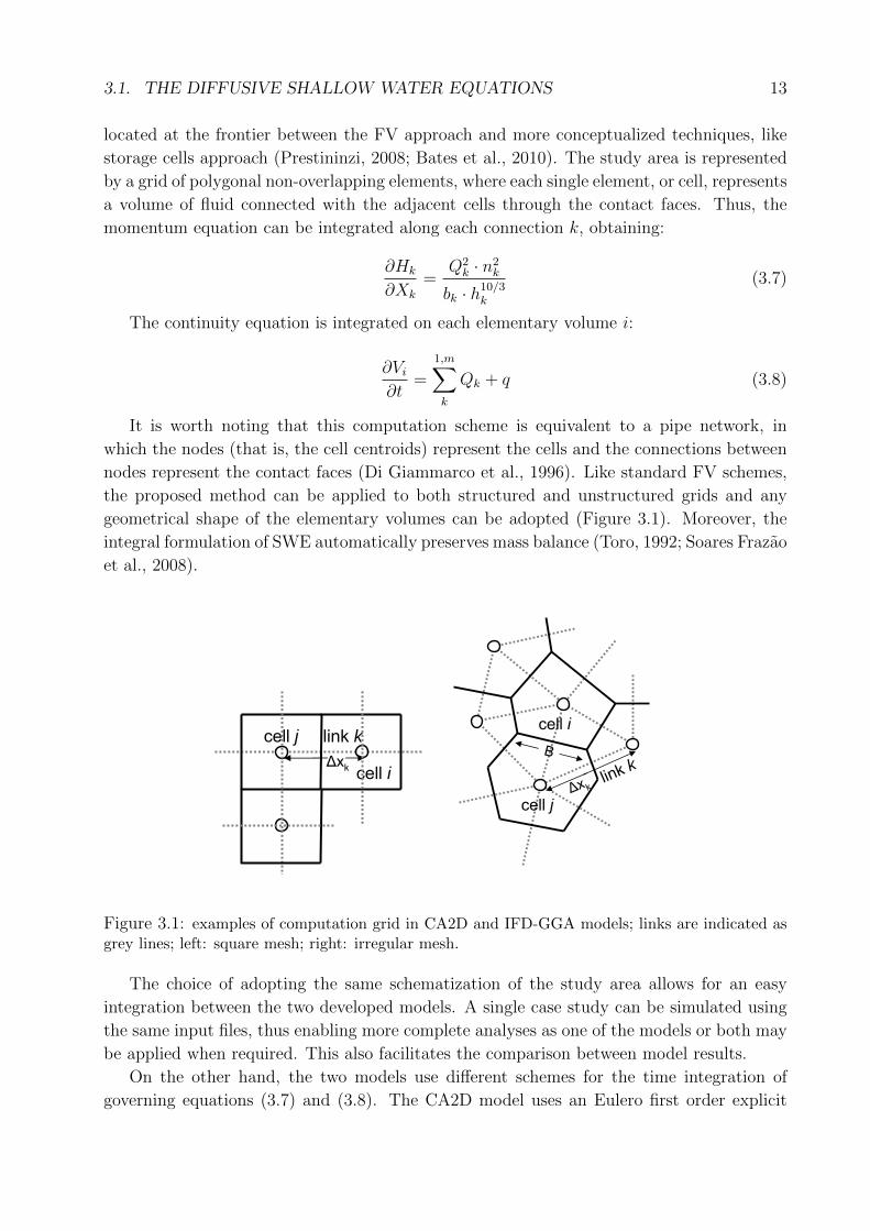
It is worth noting that this computation scheme is equivalent to a pipe network, in
which the nodes (that is, the cell centroids) represent the cells and the connections between
nodes represent the contact faces (Di Giammarco et al., 1996). Like standard FV schemes,
the proposed method can be applied to both structured and unstructured grids and any
geometrical shape of the elementary volumes can be adopted (Figure 3.1). Moreover, the
integral formulation of SWE automatically preserves mass balance (Toro, 1992; Soares Frazao
et al., 2008).
schema di calcolo AC: griglie delle connessionischema di calcolo AC: griglie delle connessioni
cell i
cell j
link kB
∆x k
cell i
cell j link k
B
∆xk
∆x∆x
schema di calcolo AC: griglie delle connessionischema di calcolo AC: griglie delle connessioni
cell i
cell j
link kB
∆x k
cell i
cell j link k
B
∆xk
∆x∆x
Figure 3.1: examples of computation grid in CA2D and IFD-GGA models; links are indicated asgrey lines; left: square mesh; right: irregular mesh.
The choice of adopting the same schematization of the study area allows for an easy
integration between the two developed models. A single case study can be simulated using
the same input files, thus enabling more complete analyses as one of the models or both may
be applied when required. This also facilitates the comparison between model results.
On the other hand, the two models use different schemes for the time integration of
governing equations (3.7) and (3.8). The CA2D model uses an Eulero first order explicit
14 CHAPTER 3. DEVELOPED MODELS
scheme, while the IFD-GGA model uses an implicit Crank-Nicholson scheme, with a weight
coefficient θ (Di Giammarco et al., 1996).
Being explicit in time, the CA2D model is expected to be much faster than the implicit
IFD-GGA model, in which an equation system must be solved at each time step. However,
overall computational efficiency can be comparable since the latter is unconditionally stable
and therefore can use larger time steps (Di Giammarco et al., 1996). In addition, the CA2D
scheme is first order accurate in time, while in the IFD-GGA model the accuracy should
depend on the weight coefficient θ.
On the other hand, implicit models may be subject to a number of drawbacks that
explicit schemes don’t have:
• At each time step, a linear system needs to be solved: the approximation introduced
in the required iterative solution can result in a loss of precision as the simulation
proceeds in time, although time step solution is still convergent.
• Although implicit models are unconditionally stable, the time step can not be arbit-
rarily large, and must be chosen case by case according to boundary and internal flow
conditions in order to preserve accuracy; therefore a standard criteria for time step
selections is difficult to establish. On the contrary, explicit models can be based on ap-
propriate stability criteria that allow for the implementation of adaptive time stepping
techniques (see Section 3.2.4).
Resuming, the feasibility of each model should be carefully tested in different conditions.
Thus, these issues will be further discussed in Chapter 4.
3.2 The CA2D model
The CA2D model here described can be considered a tradeoff between physically based finite
volume models and empirical cellular automata models. A cellular automaton (pl. cellular
automata, abbrev. CA) is a discrete model for the description of physical dynamic systems
regulated only by local laws. Typically it consists of a regular grid of cells, each in one of a
finite number of states or properties, such as ”on” and ”off”. For each cell, a set of cells called
its neighborhood (usually including the cell itself) is defined. An initial state is selected by
assigning a state for each cell. The system evolves in time according to some fixed rule
(generally, a mathematical function) that determines the new state of each cell in terms of
the current state of the cell and the states of the cells in its neighborhood. Typically, the
rule for updating the state of cells is the same for each cell and does not change over time,
and is applied to the whole grid simultaneously (Wikipedia, 2012)
Cellular automata are currently used to model several physical phenomena, when either
the complexity of the governing equations or data scarcity prevent detailed simulations.
Current fields of application include computability theory, mathematics, physics, complexity
science, theoretical biology and microstructure modelling. In particular, CA have also been
used to simulate specific fluid dynamics phenomena like debris flows (D’Ambrosio et al.,
3.2. THE CA2D MODEL 15
2003), pyroclastic flows (Avolio et al., 2006), infiltration and water surface flow (Parsons
and Fonstand, 2007). In these applications the so called macroscopic cellular automata
approach was applied, which partly differs from the classical CA structure so far described.
The cell lattice of a macroscopic CA forms a grid of polygonal elements of either regular
or variable shape and dimension, which represents the topography of the study area. In
fluid dynamics applications, each cell represents a volume of fluid to which either empirical
relationships or physically based equations may be applied. It is worth noting that in some
specific fluid dynamics applications (e.g. sand transport by wind) discrete CA models were
used (Chopard and Masselot, 1999). Although potentially interesting, this approach is not
feasible when systems composed by huge numbers of particles have to be reproduced, like in
usual large scale problems of surface flow.
Given this reference background, it was decided to develop a hydraulic model based on
macroscopic cellular automata approach and the diffusive equations. Previous CA models
for surface flow were based either on simplified equations (e.g. Manning uniform flow equa-
tion) or approximated SWE (Parsons and Fonstand, 2007). The diffusive approximation
is particularly suited to be used within a CA model: by eliminating inertial terms, flow
becomes a function of water levels and the structure of 2D flow can be heavily simplified
while preserving a considerable amount of “physics” in the model. For example, the diffusive
approximation allows to decouple flow components.
From a practical point of view, the combination of diffusive equations and macroscopic
CA leads to a simplified finite volume scheme, as mentioned in Section 3.1.1.
3.2.1 CA2D diffusive version
In the first version of the CA model scheme, the integration in time is obtained with the
Euler first order explicit scheme, following the CA rule that the overall system state only
depends on the previous time step. Thus, the continuity equation (3.8) is discretized at time
step t+ ∆t as:
V t+∆ti = V t
i + ∆tm∑j=1
Qti,j +Qt
0 (3.9)
where ∆t is the time step in use and Q0 is the total discharge entering or exiting the
domain through cell i. Considering two adjacent cells i and j, the discharge Q through the
contact face is given by the momentum equation:
Qi,j =Bh
5/3m
n
(Hi −Hj
∆x
)1/2
(3.10)
whereHi, Hjare the water stages in the two cells; ∆x is the distance between centroids
of the two cells; B is the width of the contact face; n is the Manning roughness coefficient;
hm is the arithmetic mean between water depths in the two cells. The reasons for choosing
this specific water depth value are reported in detail in Section 3.4.1.
As the momentum equation (3.7) is integrated along the link direction, any generic 2D
16 CHAPTER 3. DEVELOPED MODELS
flow is decomposed in 1D flow components through the links, ∆x being a vector with x and
y components. Each flux component is therefore decoupled from the others, so that Eq.
(3.10) may be solved separately for each link.
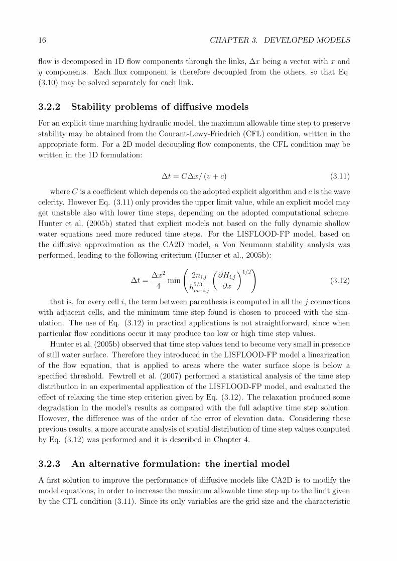
3.2.2 Stability problems of diffusive models
For an explicit time marching hydraulic model, the maximum allowable time step to preserve
stability may be obtained from the Courant-Lewy-Friedrich (CFL) condition, written in the
appropriate form. For a 2D model decoupling flow components, the CFL condition may be
written in the 1D formulation:
∆t = C∆x/ (v + c) (3.11)
where C is a coefficient which depends on the adopted explicit algorithm and c is the wave
celerity. However Eq. (3.11) only provides the upper limit value, while an explicit model may
get unstable also with lower time steps, depending on the adopted computational scheme.
Hunter et al. (2005b) stated that explicit models not based on the fully dynamic shallow
water equations need more reduced time steps. For the LISFLOOD-FP model, based on
the diffusive approximation as the CA2D model, a Von Neumann stability analysis was
performed, leading to the following criterium (Hunter et al., 2005b):
∆t =∆x2
4min
(2ni,j
h5/3m−i,j
(∂Hi,j
∂x
)1/2)
(3.12)
that is, for every cell i, the term between parenthesis is computed in all the j connections
with adjacent cells, and the minimum time step found is chosen to proceed with the sim-
ulation. The use of Eq. (3.12) in practical applications is not straightforward, since when
particular flow conditions occur it may produce too low or high time step values.
Hunter et al. (2005b) observed that time step values tend to become very small in presence
of still water surface. Therefore they introduced in the LISFLOOD-FP model a linearization
of the flow equation, that is applied to areas where the water surface slope is below a
specified threshold. Fewtrell et al. (2007) performed a statistical analysis of the time step
distribution in an experimental application of the LISFLOOD-FP model, and evaluated the
effect of relaxing the time step criterion given by Eq. (3.12). The relaxation produced some
degradation in the model’s results as compared with the full adaptive time step solution.
However, the difference was of the order of the error of elevation data. Considering these
previous results, a more accurate analysis of spatial distribution of time step values computed
by Eq. (3.12) was performed and it is described in Chapter 4.
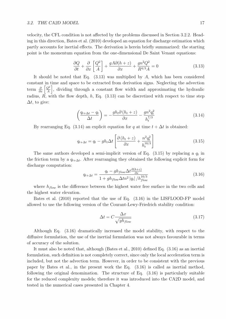
3.2.3 An alternative formulation: the inertial model
A first solution to improve the performance of diffusive models like CA2D is to modify the
model equations, in order to increase the maximum allowable time step up to the limit given
by the CFL condition (3.11). Since its only variables are the grid size and the characteristic
3.2. THE CA2D MODEL 17
velocity, the CFL condition is not affected by the problems discussed in Section 3.2.2. Head-
ing in this direction, Bates et al. (2010) developed an equation for discharge estimation which
partly accounts for inertial effects. The derivation is herein briefly summarized: the starting
point is the momentum equation from the one-dimensional De Saint Venant equations:
∂Q
∂t+
∂
∂x
[Q2
A
]+gA∂(h+ z)
∂x+gn2Q2
R4/3A= 0 (3.13)
It should be noted that Eq. (3.13) was multiplied by A, which has been considered
constant in time and space to be extracted from derivation signs. Neglecting the advection
term ∂∂x
[Q2
A
], dividing through a constant flow width and approximating the hydraulic
radius, R, with the flow depth, h, Eq. (3.13) can be discretized with respect to time step
∆t, to give: (qt+∆t − qt
∆t
)= −ght∂ (ht + z)
∂x− gn2q2
t
h7/3t
(3.14)
By rearranging Eq. (3.14) an explicit equation for q at time t+ ∆t is obtained:
qt+∆t = qt − ght∆t
[∂ (ht + z)
∂x+n2q2
t
h10/3t
](3.15)
The same authors developed a semi-implicit version of Eq. (3.15) by replacing a qt in
the friction term by a qt+∆t. After rearranging they obtained the following explicit form for
discharge computation:
qt+∆t =qt − ghflow∆t∂(h+z)
∂x
1 + ghflow∆tn2 |qt| /h10/3flow
(3.16)
where hflow is the difference between the highest water free surface in the two cells and
the highest water elevation.
Bates et al. (2010) reported that the use of Eq. (3.16) in the LISFLOOD-FP model
allowed to use the following version of the Courant-Lewy-Friedrich stability condition:
∆t = C∆x√ghflow
(3.17)
Although Eq. (3.16) dramatically increased the model stability, with respect to the
diffusive formulation, the use of the inertial formulation was not always favourable in terms
of accuracy of the solution.
It must also be noted that, although (Bates et al., 2010) defined Eq. (3.16) as an inertial
formulation, such definition is not completely correct, since only the local acceleration term is
included, but not the advection term. However, in order to be consistent with the previous
paper by Bates et al., in the present work the Eq. (3.16) is called as inertial method,
following the original denomination. The structure of Eq. (3.16) is particularly suitable
for the reduced complexity models; therefore it was introduced into the CA2D model, and
tested in the numerical cases presented in Chapter 4.
18 CHAPTER 3. DEVELOPED MODELS
3.2.4 The introduction of a local time step algorithm
Why a local time step algorithm? A further method to improve the performance of a
hydraulic model is discussed in this section.
The great majority of explicit time marching hydraulic models include an algorithm for
modifying the current time step according to flow conditions, in order to use, during the
simulation, the greatest value which guarantees stability over the whole computation grid.
The time step is usually adapted considering both theoretical criteria, based on the stability
analysis (e.g. the CFL condition), and empirical controls (e.g. a maximum value of water
depth change in a cell during a single time step).
The use of a global, adaptive time step (GTS) has a major drawback, especially in the
presence of concentrated flow areas and complex topography, or when using unstructured
meshes with large variations on cell size: the time step can locally assume values that are
significantly smaller than values computed in the rest of computational grid, thus resulting
in a considerable slowing of the simulation.
A viable approach to overcome this problem is through the use of local adaptive time step
(LTS) for the time marching of simulation, whereby each grid cell is integrated according to
the local flow physics and numerical stability (Kleb and Batina, 1992).
Early results on local time stepping have been published by Osher and Sanders (1983)
for one-dimensional scalar conservation laws and, since then, many LTS methods have been
proposed for numerical models solving the Euler and Navier-Stokes equations. In the field
of hydraulic engineering, local time stepping tecniqhes has demonstrated utility both in
1D channel flow modeling (Crossley et al., 2003) and in 2D applications involving irregular
topography and wetting and drying processes (Sanders, 2008). In both works, the local time
step algorithm increased the computational efficiency from 25% to 70% with respect to GTS
methods, with no loss in accuracy.
LTS techniques were first developed and implemented in models with unstructured
meshes and local grid refinement schemes. However, according to Sanders (2008) and Cross-
ley et al. (2003), models that use a uniform grid may also benefit from LTS schemes in
applications involving a variable wave speed.
The implementation of a LTS algorithm within CA2D could be particularly favourable,
since the diffusive stability condition (3.6)implies the use of locally small time steps. Hence,
a local time step algorithm based on an existing method has been implemented within the
CA2D model and is described here.
The proposed local time step formulation. The implementation of a local time step
is obviously not straightforward: in order to maintain a time-accurate solution, a method
of accurately exchanging information between cells being integrated at disparate time steps
needs to be developed (Kleb and Batina, 1992).
Several methods for managing interface between regions at different time steps have
been proposed in literature. Kleb and Batina (1992) presented a LTS technique based
upon advancing individual cells to the level allowed by the CFL condition, then using linear
interpolation at the interface to extract the information at the correct point in time. A
3.2. THE CA2D MODEL 19
similar approach was used by Sanders (2008), whereas Muller and Stiriba (2007) used a
predictor-corrector approach to compute fluxes at the interface.
All these techniques require to identify regions where cells are integrated with the same
specific time step, and to define interfaces between regions where time integration has to
change gradually. In addition, in order to avoid numerical errors the ratio between min-
imum and maximum time step needs to be limited (Crossley et al., 2003; Sanders, 2008).
This results in an increase of computation cost and complication of code, although all the
mentioned authors reported considerable increases in overall code speed.
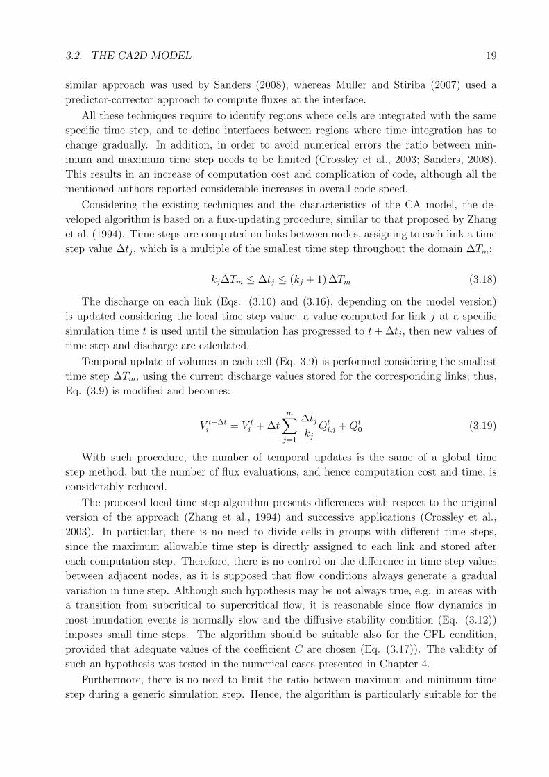
Considering the existing techniques and the characteristics of the CA model, the de-
veloped algorithm is based on a flux-updating procedure, similar to that proposed by Zhang
et al. (1994). Time steps are computed on links between nodes, assigning to each link a time
step value ∆tj, which is a multiple of the smallest time step throughout the domain ∆Tm:
kj∆Tm ≤ ∆tj ≤ (kj + 1) ∆Tm (3.18)
The discharge on each link (Eqs. (3.10) and (3.16), depending on the model version)
is updated considering the local time step value: a value computed for link j at a specific
simulation time t is used until the simulation has progressed to t+ ∆tj, then new values of
time step and discharge are calculated.
Temporal update of volumes in each cell (Eq. 3.9) is performed considering the smallest
time step ∆Tm, using the current discharge values stored for the corresponding links; thus,
Eq. (3.9) is modified and becomes:
V t+∆ti = V t
i + ∆tm∑j=1
∆tjkj
Qti,j +Qt
0 (3.19)
With such procedure, the number of temporal updates is the same of a global time
step method, but the number of flux evaluations, and hence computation cost and time, is
considerably reduced.
The proposed local time step algorithm presents differences with respect to the original
version of the approach (Zhang et al., 1994) and successive applications (Crossley et al.,
2003). In particular, there is no need to divide cells in groups with different time steps,
since the maximum allowable time step is directly assigned to each link and stored after
each computation step. Therefore, there is no control on the difference in time step values
between adjacent nodes, as it is supposed that flow conditions always generate a gradual
variation in time step. Although such hypothesis may be not always true, e.g. in areas with
a transition from subcritical to supercritical flow, it is reasonable since flow dynamics in
most inundation events is normally slow and the diffusive stability condition (Eq. (3.12))
imposes small time steps. The algorithm should be suitable also for the CFL condition,
provided that adequate values of the coefficient C are chosen (Eq. (3.17)). The validity of
such an hypothesis was tested in the numerical cases presented in Chapter 4.
Furthermore, there is no need to limit the ratio between maximum and minimum time
step during a generic simulation step. Hence, the algorithm is particularly suitable for the

20 CHAPTER 3. DEVELOPED MODELS
spatial distribution of time steps given by Eq. (3.12). For example, considering a levee
breach simulation, the minimum time step may be less than 0.1s near the inflow area, due
to high water depths and rapidly varying flow, while the maximum value may be 10 seconds
in areas with low water depths or still water.
The only limitation introduced in the algorithm regards the minimum and maximum al-
lowable time step (normally 0.01s and 10-20s), which are necessary considering the numerical
problems given by the diffusive stability condition (see Section 3.2.2).
3.3 The IFD-GGA model
The model here described is a modification of the original Integrated Finite Differences (IFD)
model developed at the Department of Earth, Environmental and Geological Sciences. In the
original version of the IFD model, the solution algorithm was based on a dichotomic iterative
scheme, while the resulting equation system was solved with a modified conjugate gradient
method (Commission EC, 1996; Di Giammarco et al., 1996). The resulting scheme is stable
and convergent in any situation, and the model was successfully used for the analysis of
flood scenarios (Commission EC, 1996; Anselmo et al., 1996). However, the low convergence
speed limited practical application of the model.
In order to overcome this problem, it was decided to rewrite the model code, incorporating
a new solution algorithm derived from the Global Gradient Algorithm (Todini and Pilati,
1988), used for pipe network analysis. Consequently the new model has been named IFD-
GGA. We consider the system of equations (3.7) and (3.8) rewritten as follows:n2|Q|Q
B2i,j(H−Z)10/3 = −∂H
∂x
Ωi∂hi∂t
=∑ni
k=1Qij +Q0i
(3.20)
The system of equations (3.20) is discretized on space and time obtaining:
37
n2i,j |Qij,t|Qij,t
B2i,j
(h−7/3i −h−7/3
j
)t
(hj−hi)t− hi,t−hj,t
∆Xi,j− S0 = 0
Ωihi,t−hi,t−∆t
∆t− θ
(∑nik=1 Qij +Q0i
)t− (1− θ)
(∑nik=1Qij +Q0i
)t−∆t
= 0(3.21)
where θ is the weight coefficient of the the implicit Crank-Nicholson scheme (Di Giam-
marco et al., 1996). Please note that the momentum equation has been integrated in space
along a generic link by using an integral average of head losses (see Section 3.4.1). The
equation system (3.21) can be written in a matrix notation, extending the original GGA
algorithm (Todini and Pilati, 1988) to the unsteady flow condition: A11... A12
· · · · · ·A21
... A22
Q
H
=
−A10H0
−Q∗
(3.22)
3.3. THE IFD-GGA MODEL 21
The elements in system (3.22) are herein described:
Qt = [Q1,t, Q2,t, · · · , Qnp,t] is the vector of discharges [1, np],
Ht = [H1,t, H2,t, · · · , Hnp,t] is the vector of unknown water stages [1, nn],
Ht = [Hnn+1,t, Hnn+2,t, · · · , Hntot,t] is the vector of known water stages [1, ntot],
Qt∗ = [Q∗1,t, Q∗2,t, · · · , Q∗np,t] is the vector of known terms [1, nn − ntot],where (np) is the number of links, (nn) is the number of nodes with unknown water stage,
(ntot) is the total number of nodes, (nn − ntot) is the number of nodes with known water
stage.
A11 is a diagonal matrix with dimension [np, np] where the elements are defined as:
A11 (k, k) =3
7
n2i,j |Qi,j|B2i,j
(h−7/3i − h−7/3
j
)(hj − hi)
(3.23)
The formulation (3.23) must be modified when ε = (hi − hj)→ 0 ; we have therefore:
A11 =n2i,j |Qi,j|∆xB2i,j
h−10/3 (3.24)
A22 is a diagonal matrix with dimension [nn, nn] where the elements are defined as:
A22 (i, i) = − Ωi
θ∆t(3.25)
The generic element of the vector Q∗t is defined as:
Qt ∗ (i) = Qi,t +Ωi
θ∆tHi,t−∆t +
(1− θ)θ
(nn∑k=1
Qk +Q0i
)t−∆t
(3.26)
The topology of the network (nodes and links) is described by matrix A12, defined as:
A12 (i, k) =
−1 if flow in the link k leaves node i
0 if link k doesn′t include node i
+1 if flow in the link k enters node i
In order to guarantee the existence of a unique solution, the water elevation must be known
in at least one cell. This implies the partition of A12 in two sub-matrices:
A12 =[A12
... A10
]where A12 = AT21 describes the links between the unknown water head nodes, while
A10 = AT01 describes the links with the known head nodes.
3.3.1 Newton-Raphson and Jacobi methods
In order to speed up the solution algorithm of the original IFD model, different approaches
have been developed. In the first one, the original dichotomic method has been substituted
22 CHAPTER 3. DEVELOPED MODELS
with the Newton-Raphson (NR) method, coupled with the Jacobi method to solve the inner
iterative cycle (Kelley, 1995; Luenberger, 2003). In order to apply the NR method, the Eqs.
(3.21) must be differentiated on Qij,t,hi,t,hi,t−∆t, obtaining the following expressions:
67
n2i,j∆Xi,j |Qij,t|
B2i,j
(h−7/3i −h−7/3
j
)t
(hj−hi)tdQij,t − 1+
+n2i,j |Qij,t|Qij,t∆x
B2i,j
(37
(h−7/3i −h−7/3
j
)(hj−hi)2 − h
−10/3i
(hj−hi)
)t
dhi,t+
+1− n2i,j |Qij,t|Qij,t∆x
B2i,j
(37
(h−7/3i −h−7/3
j
)(hj−hi)2 − h
−10/3j
(hj−hi)
)t
dhj,t = dEij,t∑nik=1Qij,t − Ωi
θ∆tdhi,t = dEi,t
(3.27)
where: dEij,t = 37
n2i,j∆Xi,j |Qij,t|Qij,t
B2i,j
(h−7/3i −h−7/3
j
)t
(hj−hi)t− (hi − hj)t −∆Xi,jS0i,j
dFij,t =∑ni
k=1 Qij,t − Ωi
θ∆t(hi,t − hi,t−∆t) +Q0i,t − (1−θ)
θ
(∑nik=1Qij +Q0i
)t−∆t
(3.28)
It is possible to write the two differentials in a matrix form as:dEτ = Aτ
11Qτ + A12hτ + Aτ1oh0 − S
dFτ = A21Qτ + Aτ22hτ + Q∗ (3.29)
where τ is the iteration index and S is a vector whose elements are defined as:
S (k) = ∆xijS0,ij (3.30)
The non symmetric system (3.29) can be written in matrix to derive the solving algorithm:[Dτ
11 Dτ12
A21 Aτ22
] [dQτ
dhτ
]=
[dEτ
dFτ
](3.31)
where, omitting the τ index for sake of clarity:
D11 =6
7
n2i,j
∣∣Qi,j
∣∣∆xB2i,j
(h−7/3i − h−7/3
j
)(hj − hi)
= 2A11 (3.32)
D12 (k, i) = −1 +n2i,j |Qi,j|Qi,j∆x
B2i,j
3
7
(h−7/3i − h−7/3
j
)(hj − hi)2 − h
−10/3i
(hj − hi)
(3.33)
D12 (k, j) = 1−n2i,j |Qi,j|Qi,j∆x
B2i,j
3
7
(h−7/3i − h−7/3
j
)(hj − hi)2 −
h−10/3j
(hj − hi)
(3.34)
Where nodes i, j indicate respectively the starting and ending node of link k. Equations
(3.32), (3.33), (3.34) have to be modified when ε = (hi − hj)→ 0; in this case we have:
3.3. THE IFD-GGA MODEL 23
A11 =2n2
i,j |Qi,j|∆xB2i,j
h−10/3 (3.35)
D12 (k, i) = −1−5n2
i,j |Qi,j|Qi,j∆x
3B2i,j
(h−13/3i
)(3.36)
D12 (k, j) = 1−5n2
i,j |Qi,j|Qi,j∆x
3B2i,j
(h−13/3j
)(3.37)
The solution of the linear equation system can be obtained once the inverse of the system
matrix is found: [D11 D12
A21 A22
] [B11 B12
B21 B22
]=
[I 0
0 I
](3.38)
where the iteration index τ has been omitted. From Eq. (3.38) the following relationships
can be obtained: D11B11 + D12B21 = I
D11B12 + D12B22 = 0
A21B11 + A22B21 = I
A21B12 + A22B22 = 0
(3.39)
Therefore, the analytic solution of the equation system (3.29) is:dQ = B11dE + B12dF
dh = B21dE + B22dF(3.40)
Replacing in Eq. (3.40) the formulation of the terms, after some simple algebraic passages
the increase for the water depth is:
dh =(A21D−1
11 D22 − A22
)−1··[A21
(D−1
11 A11 − I)
Q +(A21D−1
11 D22 − A22
)h + A21D−1
11 A10h0 −Q∗] (3.41)
As can be noticed, the matrix that have to be inverted is not symmetric but stricly
diagonal dominant, thanks to the sum of matrix A22 on the main diagonal. This allows
to solve the system (3.40) using iterative techniques like the Jacobi method. The analysis
of the equations shows that it is possible to replace dh in the formulation of dQ; after an
appropriate recombination of terms, dQ can be written as:
dQ = D−111 [dE−D12dh] (3.42)
that can be estimated once dh has been computed. dh is computed with the Jacobi
method as:
(A21D−1
11 D22 − A22
)dh = A21D−1
11 dE−dF (3.43)
24 CHAPTER 3. DEVELOPED MODELS
Therefore, each time step the application of the iterative Newton Raphson algorithm
performed by solving one by one the following relationships for each iteration τ :
dhτ =[A21
(Dτ−1
11
)−1D22 − A22
] [A21
(Dτ−1
11
)−1dEτ−1 − dFτ−1
]dQτ =
(Dτ−1
11
)−1 [dEτ−1 −Dτ−1
12 dhτ]
hτ = hτ−1 − dhτ
Qτ = Qτ−1 − dQτ
dEτ = A11Qτ + A12hτ + A10hτ0 − SdFτ =
[(A21Qτ + qτ ) + 1−ϑ
ϑ
(A21Qτ−1 + Q0
τ−1)]
+ A22 (hτ + hτ−1)
(3.44)
3.3.2 Linear Theory and Jacobi method
In the second solution algorithm designed for the IFD-GGA model, the equation system
(3.21) is linearised by using the Linear Theory (LT) approach (Wood and Charles, 1972).
In this case, the following recursive scheme is used, solving first for the water level and then
the discharge: Hτ =[A21
(Aτ−1
11
)−1A22 − A22
]−1 [Q ∗ −A21
(Aτ−1
11
)−1A10H0
]Qτ = 1
2
[Qτ−1 −
(Aτ−1
11
)−1(A12Hτ−A10H0)
] (3.45)
As can be noticed from Eqs. (3.45), the iterative solution requires the solution of a
system of linear equations, which matrix(A21 (Aτ
11)−1 A22 − A22
)is a sparse symmetrical
matrix with dominant diagonal. These conditions allow for the use of the recursive Jacobi
approach, instead of more direct frontal Gauss-Seidel or matrix factorization approaches.
3.3.3 Discussion
Both the proposed schemes have been chosen to provide a fast and reliable solution algorithm
for the IFD-GGA model. The Newton-Raphson scheme guarantees the fastest rate of conver-
gence among the possible schemes for solving non linear systems (Kelley, 1995; Luenberger,
2003). In theory, the Linear Theory does not provide a convergence rate comparable to NR
when high precision is required in the solution. However, in preliminary tests it was found
that, for the accuracy requirements in typical flood inundation events (around 10−3 m), the
LT approach required more or less the same number of iterations of the NR approach, with
the advantage of a resulting symmetrical system matrix to be handled (Wood and Charles,
1972).
In addition, the use of the Jacobi scheme allows to decompose the resulting equation
systems to single equations that can be solved indipendently. In this way, the algorithm can
be massively parallelized, as for an explicit scheme (see Section 3.5).
However, it should be noted that the proposed approaches are not designed to be applied
in hydraulic models like IFD-GGA. 2D hydraulic simulations can involve the solution of very
large equation systems (more than 104 equations); in addition, each time step the solution
3.4. FURTHER ASPECTS OF THE PROPOSED MODELS 25
must be computed from the previous solution, with the risk of introducing increasing errors.
Therefore the effective performance of the proposed solution schemes needs to be carefully
evaluated.
In literature, the Newton-Raphson scheme is not recommended for problems with large
number of variables (Kelley, 1995; Luenberger, 2003). Moreover, NR provides a non sym-
metric matrix, meaning that only specific algorithms can be applied to solve the resulting
linear system. The LT approach leads to a symmetrical system matrix, but the accuracy
required for the convergence, and the overall speed of the LT method with respect to the
NR method should be verified.
More problems may arise from the use of the Jacobi scheme. In fact, when the method
is applied to solve simulations over large time spans, a high precision of the solution (10−8
tolerance or less) is generally required, otherwise the error may grow as the simulation
progresses in time and the results can diverge too much from the correct solution (Kelley,
1995; Luenberger, 2003). However, such a precision would slow the convergence rate as a
large number of iteration is required. In addition, the convergence rate of the method for
large equation systems needs to be verified.
In Section 4, all these possible drawbacks are analyzed and discussed in detail.
3.4 Further aspects of the proposed models
The two proposed models share a number of features that are described more in detail in this
section. In addition, the section includes the explanation of some specific modeling details.
3.4.1 Discretization of head losses
The choice of the formulation for computing the friction slope J has a great impact on model
performance. In order to find the best solution in terms of accuracy and stability, different
formulations have been tested within the CA2D and IFD-GGA models. Table 3.1 reports a
number of alternative formulations that were obtained considering a linear variation of the
water depth along a generic link; Table 3.2 reports other formulations developed under the
hypothesis of a logarithmic variation of water depth.
The formulations were tested in different numerical cases, some of which are reported
in Chapter 4 (cases 2 and 3); these simulations included 1D and 2D flow conditions over
different bed slopes. For the CA2D diffusive version, the best result in terms of correct flow
propagation was obtained using the arithmetic mean hm in Eq. (3.10), that is, considering
a linear variation of the water depth along a generic link, and computing head losses in the
middle section (Eq. (3.46) in Table 3.1). It is interesting to note that in the LISFLOOD-
FP model, which is similar to CA2D, a different reference value for water depth is used.
The reference value hflow (Section 3.2.3) is defined as the difference between the highest
water free surface in the two cells and the highest water elevation (Bates et al., 2010). Such
formulation was chosen by the developers of the LISFLOOD-FP model because the use
of hm produced highly unstable results for all except horizontal planes, while the use of
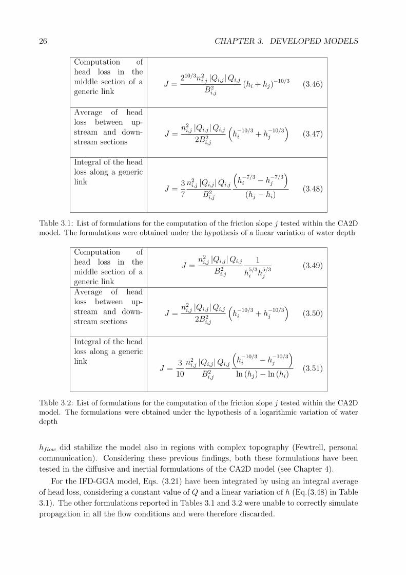
26 CHAPTER 3. DEVELOPED MODELS
Computation ofhead loss in themiddle section of ageneric link
J =210/3n2
i,j |Qi,j|Qi,j
B2i,j
(hi + hj)−10/3 (3.46)
Average of headloss between up-stream and down-stream sections
J =n2i,j |Qi,j|Qi,j
2B2i,j
(h−10/3i + h
−10/3j
)(3.47)
Integral of the headloss along a genericlink
J =3
7
n2i,j |Qi,j|Qi,j
B2i,j
(h−7/3i − h−7/3
j
)(hj − hi)
(3.48)
Table 3.1: List of formulations for the computation of the friction slope j tested within the CA2Dmodel. The formulations were obtained under the hypothesis of a linear variation of water depth
Computation ofhead loss in themiddle section of ageneric link
J =n2i,j |Qi,j|Qi,j
B2i,j
1
h5/3i h
5/3j
(3.49)
Average of headloss between up-stream and down-stream sections
J =n2i,j |Qi,j|Qi,j
2B2i,j
(h−10/3i + h
−10/3j
)(3.50)
Integral of the headloss along a genericlink
J =3
10
n2i,j |Qi,j|Qi,j
B2i,j
(h−10/3i − h−10/3
j
)ln (hj)− ln (hi)
(3.51)
Table 3.2: List of formulations for the computation of the friction slope j tested within the CA2Dmodel. The formulations were obtained under the hypothesis of a logarithmic variation of waterdepth
hflow did stabilize the model also in regions with complex topography (Fewtrell, personal
communication). Considering these previous findings, both these formulations have been
tested in the diffusive and inertial formulations of the CA2D model (see Chapter 4).
For the IFD-GGA model, Eqs. (3.21) have been integrated by using an integral average
of head loss, considering a constant value of Q and a linear variation of h (Eq.(3.48) in Table
3.1). The other formulations reported in Tables 3.1 and 3.2 were unable to correctly simulate
propagation in all the flow conditions and were therefore discarded.
3.4. FURTHER ASPECTS OF THE PROPOSED MODELS 27
3.4.2 Computation of velocity
In CA2D and IFD-GGA codes, velocity values are derived from the discharge values com-
puted on the connections and divided by the link cross section A (the reference water depth
value is discussed in Section 3.4.1). To obtain a consistent velocity field on the computation
grid, velocities are then associated to each cell by means of a weighted vectorial average. For
each cell i that has np connections to the adjacent cells, the average is performed separately
on the x and y directions:
Uxi =
∑npj=1 (cos (j)Uj)∑np
j=1 cos (j)(3.52)
Uyi =
∑npj=1 (sin (j)Uj)∑np
j=1 sin (j)(3.53)
where Uxj, Uyj are the computed velocity components for cell i and sin (j), cos (j) indicate
the direction of the connection j (x and y components are assumed to be positive in eastward
and northward direction respectively). Eqs. (3.52) and (3.53) allow to easily compute the
velocity field either for regular or irregular grids.
3.4.3 Simulation of wetting and drying processes
One of the most complex issues related to flood inundation modelling is the correct treatment
of wetting and dying processes. Standard numerical procedure for solving SW equations may
produce unphysical oscillations and negative water depths near a dry/wet front (Arico et al.,
2011). Consequently, hydrodynamic models are generally equipped with specific wetting–
drying (WD) algorithms. It is important to note that hydraulic models based on implicit
time marching schemes generally require more complex WD algorithms, since large equation
systems have to be solved each time step; WD treatment is instead simplified in explicit
models. Although some methods track the WD interfaces in time, moving the boundary
nodes and deforming accordingly the computational mesh, most of the available WD methods
adopt a fixed mesh (Arico et al., 2011). In some of these methods, mesh elements (nodes or
cells) are activated or deactivated according to their wet-dry condition, while other methods
introduce transition elements (partially wet) to describe WD interface.
However, the application of complex algorithms for WD treatment can be not convenient,
especially for reduced complexity models. Apart from fast propagating wetting fronts, like
those produced by a dam break or in the proximity of a levee breach, during an inundation
event wetting fronts are usually slow, wide extended and with reduced water depths, and are
therefore similar to a rainfall induced overland flow. According to different authors (Horton
, 1945; Guy et al., 1992; Bagarello and Ferro, 2006), such a condition is characterized by a
mixture of laminar and turbolent flow in which infiltration, surface roughness and rainfall
intensity play a major role (Bateman et al., 2010). Also, the gradually varied flow assumption
can be not satisfied because of perturbation produced by microtopography, and the shallow
water equations can lose validity (Tayfur et al., 1993). Drying processes are also strongly
influenced by these factors, and their treatment is in some ways more problematic than of
28 CHAPTER 3. DEVELOPED MODELS
the wetting front (Horritt, 2002).
Therefore, the use of simplified relationships to handle WD effects can be a reasonable
alternative. In fact, it should be considered that in actual flood events the quality of ex-
perimental data is rarely sufficient to assess model results, therefore a detailed reproduction
of all the mentioned processes would be scarcely useful (Horritt, 2002; Hunter et al., 2007;
Neal et al., 2009a).
A current solution, adopted both by reduced complexity models and more complex mod-
els, is the use of a threshold value on water depth to distinguish dry and wet cells (e.g. the
CCHE2D model, Jia and Wang (2001)). This simulates the surface storage effect due to
terrain roughness. In addition, in presence of reduced water depth the ordinary flow equa-
tions can be linearized or substituted with an empiric relationship (e.g. the LISFLOOD-FP
model, Hunter et al. (2005b)).
Given all these considerations, the treatment of WD processes has been undertaken with
different methods in the two developed models.
WD treatment in CA2D. In the CA2D model, wetting fronts can be directly reproduced
by the ordinary flow equations, thanks to the explicit solution scheme. Drying effects are
handled by including a control on volumes at each discharge calculation step, to ensure
mass conservation and prevent negative values of water depth. When a negative depth is
detected in a cell, the outgoing discharges are reduced so that total outgoing discharge equals
the available water volume. Incoming discharges are not modified, and the ratio between
outgoing discharges is mantained after reduction. In addition, a surface storage value may
also be used to distinguish between dry and wet cells. Each time step the control of volumes
is performed iteratively until negative depths either disappear or are kept below a tolerance
threshold (usually 10−12). The fast convergence of this method has been extensively tested
in cases with both regular and complex topography (see Chapters 4 and 5).
It must be noted that the volume control adopted within the CA2D model differs from
ordinary flow limiting techniques. Generally, flow limiters are used to prevent oscillations
of discharge values in deep water areas, and it was observed that such technique influences
model results, that become highly sensitive to grid cell size and insensitive to surface rough-
ness Hunter et al. (2005b). On the contrary, the volume control is applied in the model only
in drying conditions, that is, where water depths are very reduced. Several tests on different
flood scenarios have been performed and no significant instabilities were observed.
Thanks to the explicit solution scheme and the described drying algorithm, the CA2D
model structure can deal with large variations of flow domain without stability problems.
This is particularly useful when simulating rainfall-runoff process and infiltration (see Chapter
6).
WD treatment in IFD-GGA. In the IFD-GGA model, the treatment of WD processes
is more complicated, since the governing equations (3.21) are defined only for positive (non-
zero) water depths. This means that a minimum threshold for water depth must be estab-
lished, and consequently the equation system must include all the grid cells at each time

3.4. FURTHER ASPECTS OF THE PROPOSED MODELS 29
step. In order to minimize the additional computational burden derived from large dry
areas within the computation grid, a control on fluxes has been inserted, so that no flux
interchange is produced between cells with a water depth equal to the threshold value. A
second important problem is the threshold value can significantly influence propagation of
wetting and drying front. Although a very low value can be set (e.g. 10−6), the effect on
flow propagation and on convergence speed of the code need to be carefully evaluated. This
issue will be discussed in Chapter 4.
3.4.4 Simulation of infiltration
During lowland flood events infiltration is generally neglected. In fact, in such events infilt-
ration is much slower than surface flow processes, and soils are usually saturated with water,
resulting in very small infiltration rates. Therefore this process is currently implemented
in the two proposed models using a rather simplified approach. When soil infiltration is
activated in the model code, a special connection is added to each cell to represent the flow
of water into the soil. Every time step, infiltration rate is equal to the hydraulic conductivity
specified for each cell, until a threshold value that represents soils saturation is reached and
infiltration stops.
3.4.5 Boundary and internal conditions
In the CA2D model, the ordinary flow condition of free surface 2D flow is represented
by Eqs. (3.10) or (3.16) depending on model version, while for IFD-GGA the same flow
condition is given by Eqs (3.21). As it is immediate to see, these equations describe the
free surface 1D flow over a wide rectangular cross section with negligible lateral friction.
This approximation is usually adopted by flood inundation models, and can be considered
reasonable if no significant terrain slopes or no relevant vertical obstacles are present in the
computation domain (however, Section 5.4 presents a case study where these conditions do
not hold).
Wherever necessary, uniform or weir flow may also be imposed on specific connections. In
CA2D, the uniform flow condition for a connection k which conveys flow out of the domain
from cell i is written as:
Q0i =bh
5/3i
n
√∆Z
∆x(3.54)
For the IFD-GGA model, this flow condition is inserted in matrix A11 as:
A11 (k) =|Qk|n2
k
S0B2k (Hi − Zi)7/3
(1− Zi
Hi
) (3.55)
while the corresponding elements of matrix A12 are written as A12 (k, i) = −1 and
A12 (k, j) = 0. The weir equation for an outgoing connection is written for the CA2D
model as:
30 CHAPTER 3. DEVELOPED MODELS
Q0i = αb√
2ghi (3.56)
where α is the weir coefficient. For IFD-GGA the weir equation is written in matrix A11
as:
A11 (k) =|Qk|
2µ2kgB
2k (Hi − Zi)2
(1− Zi
Hi
) (3.57)
In addition, in the CA2D model a simplified mixed weir-pressure flow condition can be
used for outlet links. Flow is computed with Eq. (3.56) up to a threshold value of water
depth, and when threshold is exceeded the following formulation is used to compute discharge
(pressurized flow out of a conduct):
Q0i = 0.99αbhi√hi (3.58)
where α is the reduction coefficient. The treatment of incoming flow boundary conditions
in the CA2D model code needs a specific description. Each time step, the inflows entering
the domain are immediately converted into water level by updating water level in boundary
cells, before computing flow exchanges within the computation grid. On the contrary, in the
IFD-GGA model inflow boundary conditions are directly included in the overall equation
system an used to iteratively compute the solution (for instance, incoming discharges are
put in the continuity equation (3.21)).
In both the models, boundary or internal conditions may be assigned to cells by imposing
specific water level or discharge hydrographs, as well as rainfall hyetographs.
3.4.6 Advantages of proposed modeling approaches
As already pointed out in Section 3.1, the two proposed are based on a model structure
that resembles a simplified finite volumes method. At the same time, this model scheme is
also assimilable to the conceptual modelling technique known as storage cell approach, that
constitutes the basis of different hydraulic models (Prestininzi, 2008).
Given this framework, the proposed models combine different modelling solutions taken
from other simple hydraulic models like LISFLOOD-FP (Hunter et al., 2005b; Bates et al.,
2010), JFLOW (Bradbrook et al., 2004) and FLO2D (FLO-2D Software Inc., 2007). It
should be noted that so far many of these modelling solutions were not available together in
a single model. In addition, the models present some original solutions for specific modeling
issues, in order to improve model parsimony and reproduction of flow dynamics.
• Computation grid: the design of the code structure takes advantage of the analogy
with a pipe network: all the information and the computation cycles are partitioned
between node elements and link elements, in order to optimize the code efficiency. In
Chapter 4, the effectiveness of such approach to speed up the models is investigated in
detail. In addition, both the two models can handle both regular and irregular meshes.
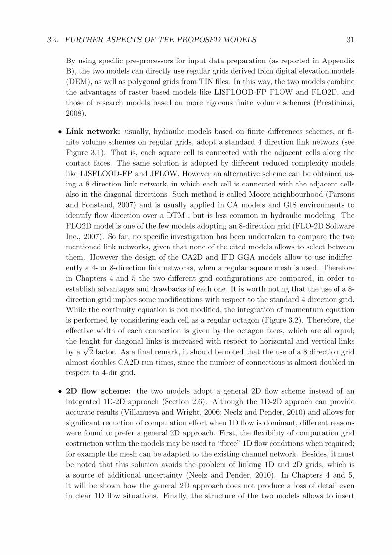
3.4. FURTHER ASPECTS OF THE PROPOSED MODELS 31
By using specific pre-processors for input data preparation (as reported in Appendix
B), the two models can directly use regular grids derived from digital elevation models
(DEM), as well as polygonal grids from TIN files. In this way, the two models combine
the advantages of raster based models like LISFLOOD-FP FLOW and FLO2D, and
those of research models based on more rigorous finite volume schemes (Prestininzi,
2008).
• Link network: usually, hydraulic models based on finite differences schemes, or fi-
nite volume schemes on regular grids, adopt a standard 4 direction link network (see
Figure 3.1). That is, each square cell is connected with the adjacent cells along the
contact faces. The same solution is adopted by different reduced complexity models
like LISFLOOD-FP and JFLOW. However an alternative scheme can be obtained us-
ing a 8-direction link network, in which each cell is connected with the adjacent cells
also in the diagonal directions. Such method is called Moore neighbourhood (Parsons
and Fonstand, 2007) and is usually applied in CA models and GIS environments to
identify flow direction over a DTM , but is less common in hydraulic modeling. The
FLO2D model is one of the few models adopting an 8-direction grid (FLO-2D Software
Inc., 2007). So far, no specific investigation has been undertaken to compare the two
mentioned link networks, given that none of the cited models allows to select between
them. However the design of the CA2D and IFD-GGA models allow to use indiffer-
ently a 4- or 8-direction link networks, when a regular square mesh is used. Therefore
in Chapters 4 and 5 the two different grid configurations are compared, in order to
establish advantages and drawbacks of each one. It is worth noting that the use of a 8-
direction grid implies some modifications with respect to the standard 4 direction grid.
While the continuity equation is not modified, the integration of momentum equation
is performed by considering each cell as a regular octagon (Figure 3.2). Therefore, the
effective width of each connection is given by the octagon faces, which are all equal;
the lenght for diagonal links is increased with respect to horizontal and vertical links
by a√
2 factor. As a final remark, it should be noted that the use of a 8 direction grid
almost doubles CA2D run times, since the number of connections is almost doubled in
respect to 4-dir grid.
• 2D flow scheme: the two models adopt a general 2D flow scheme instead of an
integrated 1D-2D approach (Section 2.6). Although the 1D-2D approch can provide
accurate results (Villanueva and Wright, 2006; Neelz and Pender, 2010) and allows for
significant reduction of computation effort when 1D flow is dominant, different reasons
were found to prefer a general 2D approach. First, the flexibility of computation grid
costruction within the models may be used to “force” 1D flow conditions when required;
for example the mesh can be adapted to the existing channel network. Besides, it must
be noted that this solution avoids the problem of linking 1D and 2D grids, which is
a source of additional uncertainty (Neelz and Pender, 2010). In Chapters 4 and 5,
it will be shown how the general 2D approach does not produce a loss of detail even
in clear 1D flow situations. Finally, the structure of the two models allows to insert
32 CHAPTER 3. DEVELOPED MODELS
schema di calcolo AC: griglie delle connessionischema di calcolo AC: griglie delle connessioni
cell i
cell j
link kB
∆x k
cell i
cell j link k
B
∆xk
∆x∆x
Figure 3.2: example of computation grid with 8 direction link network; links are indicated as greylines.
specific geometry to reproduce canalized flow in more detail; for instance, a subgrid
parameterization could be used to reproduce compound cross sections (Yu and Lane,
2011), although such possibility is still being implemented in model codes (see Chapter
6).
3.5 Parallelisation of hydraulic model codes
Parallelisation of computer codes is one of the recent lines of research to improve perform-
ances of 2D flood models (Neal et al., 2010). In a parallelised code, the computational
burden is subdivided on different processing cores that run computations in parallel, ex-
changing informations according to the parallelization method in use. Different strategies
can be applied to achieve this result.
Multiprocessor parallelisation methods use multiple general purpose CPU cores or clusters
to solve equations concurrently and thus reduce computation time. These methods are
based on message passing interface (MPI) and domain decomposition, and have been ap-
plied to different hydraulic models, including TELEMAC-2D (Hervouet, 2000),RMA (Rao,
2005), TRENT (Villanueva and Wright, 2006), LISFLOOD-FP (Neal et al., 2009b, 2010)
and FloodMap-Parallel (Yu, 2010). Basically, the domain decomposition approach breaks
the model domain into a number of contiguous sub-domains, with each sub-domain running
on a different processing core. The speedup obtained with respect to serial model versions
varied from 3.8x (Rao, 2005) to 6.2x (Hervouet, 2000) to 15x (Yu, 2010) according to the
case study, the model code and the machines used for parallelisation.
An alternative method is to couple a programmable coprocessor with a general purpose
CPU to handle computationally intensive tasks. The most common coprocessors are graphics
processing units (GPUs), which are dedicated to performing the computation associated
with graphics processing. GPUs architecture offers extensive computational capabilities
when compared to conventional CPU, including massive parallelism, high memory/data

3.5. PARALLELISATION OF HYDRAULIC MODEL CODES 33
transfer between the motherboard and the GPU, and high peak single precision floating
point performance (Neal et al., 2010; Kalyanapu et al., 2011). Therefore in recent years
GPUs have been used in a wide range of scientific computing applications (General Purpose
GPU), including flood modelling. For instance, the JFLOW model (Bradbrook et al., 2004)
has recently been rewritten for GPGPUs obtaining a speedup of 112 x over the serial JFLOW
code for a test case in Glasgow, UK (Lamb et al., 2009). Neal et al. (2010) implemented
a simplified version of the LISFLOOD-FP model on ClearSpeed accelerator cards, that are
specifically designed for computationally intensive science and engineering applications. The
parallelisation method in both GPGPUs and ClearSpeed cards is based the single instruction
multiple data (SIMD), where many processing elements (PEs) perform the same task on
different data (Neal et al., 2010).
Neal et al. (2010) applied and compared some of the described parallelization techniques
using a simplified version of the LISFLOOD-FP model. The methods included programming
of multicore processors with Open-MP language and message passing interface (MPI), and
use of ClearSpeed accelerator cards. The authors observed that parallelisation on multicore
processors can be undertaken using dedicated programming language such as OpenMP Neal
et al. (2009b), allowing a relativetly straightforward code rewriting. On the contrary, applic-
ations on GPUs require specialized hardware or dedicated complex programming languages,
thus, conversion from standard CPU codes is more difficult and time consuming. How-
ever, more recent developments such as Compute Unified Data Architecture (CUDA) by
the NVIDIA Corporation are likely to reduce the effort required in programming GPUs for
scientific applications (Kalyanapu et al., 2011). CUDA is a software environment designed
to develop parallel computations, allowing straightforward data exchange between CPU and
GPU and optimizing the number of processor cores.
On the other hand, parallelisation on dedicated coprocessors allows for greater speedup
of model with respect to standard multicore processors, due to the larger number of cores
(usual GPU cards contain around 200 cores while nowadays a standard multicore computer
has 4 or 8 cores). For instance, Kalyanapu et al. (2011) obtained a speedup of 88x and 3.5x
by implementing the fully dynamic model Flood2D respectively on a 240 cores and 16 cores
NVIDIA GPU. Computation times become comparable when clusters with several multicore
processors are used (Neal et al., 2010), but such computational structures are rarely available
with respect to standard GPUs.
Neal et al. (2010) noted that the efficiency of parallelization techniques may vary ac-
cording to specific test case; for instance, models parallelised on GPUs were less efficient on
partially wet domains, due to the more difficult subdivision of the effective computational
burden.
3.5.1 Application to the proposed models
In order to perform parallelisation of a hydraulic model code, the code structure and must
be analyzed to identify which parts can be proficiently parallelised. Generally speaking,
parallelisation is effective when applied to iterations regarding the computation spatial do-
34 CHAPTER 3. DEVELOPED MODELS
main; therefore a common practice is to decompose the study area, so that computations on
each sub-domain are performed in parallel by different processors. However, care must be
taken in defining how informations can be passed between parallel computation threads, for
instance on boundaries between sub-domains. Moreover, some information must be shared
in all the domain, therefore parts of the model code cannot be parallelised (i.e. updating of
variables at each time step) (Neal et al., 2010).
According to previous research works about this topic, models based on explicit time
marching schemes like CA2D are suited to be massively parallelised (Yu, 2010; Kalyanapu
et al., 2011). In particular, parallelisation of diffusive models is relatively straightforward
as demonstrated by the applications to LISFLOOD-FP code (Neal et al., 2009b, 2010). On
the other hand, implicit schemes can only be partly parallelised, unless particular solution
schemes are adopted. As described in Section 3.3, the implementation of the Jacobi scheme
within the IFD-GGA model has been performed exactly for this reason.
Therefore, given the requirements from the Civil Protection, it was decided to convert the
model codes from Fortran to Java language. Although Java is not a scientific language and
is therefore less efficient (the model codes are written in Fortran), the advantages in terms
of model performance would be consistent. First, the conversion of the codes facilitates the
integration into the Civil Protection information system: this will allow to run simultaneous
multiple simulations on different machines, exploiting the existing network and optimizing
the availability of idle processors. Second, the Java model code could be easily adapted
to run in parallel on distributed multiprocessor machines, using the domain decomposition
technique (Yu, 2010; Neal et al., 2010).
As mentioned in Section 3.5 the implementation of model codes on GPU cards would be
more efficient, with an expected speedup of one magnitude order with respect to multipro-
cessors code (Lamb et al., 2009; Neal et al., 2010; Kalyanapu et al., 2011). However, this
application has not been undertaken for a number of practical reasons. The main motiva-
tion was the absence of specific requirements from the Civil Protection during the research
period. It was felt not convenient to start a time consuming and costly work on the par-
allelization of the codes without immediate requirements. Moreover, dedicated hardware
for parallel programming is rapidly evolving, as well as related programming languages (see
Section 3.5); therefore some of the currently used techniques could become rapidily obsol-
ete, and problems of compatibility could arise in the future. From this point of view, the
current implementation in the information system of the Civil Protection should facilitate
the updating and compatibility of the model codes (see Chapter 6).
Chapter 4
APPLICATIONS: NUMERICAL
CASES
Every hydraulic model needs to undergo a detailed evaluation process in order to define its
range of application,advantages and drawbacks. In the scientific community there is still
no wide consensus about reliability and accuracy criteria for hydraulic models (Hunter et
al., 2007), although some institutions and national agencies developed specific requirements.
For instance, the U.S. Federal Emergency Management Agency (FEMA) published a list of
numerical models meeting the requirements of the National Flood Insurance Program for
flood hazard mapping (FEMA, 2012). On the other hand, the UK Environmental Agency
(EA) developed a list of test cases to evaluate hydraulic flood models (Neelz and Pender,
2010). This latter approach has been followed to evaluate the CA2D and IFD-GGA models.
As such, in the present chapter the models are tested in several numerical cases, reprodu-
cing a wide range of flow conditions. Numerical cases allow to isolate specific flow processes,
and to assess the computation scheme under simplified and well controlled conditions, redu-
cing the number of variables to be considered and the uncertainty concerning their influence
on model performance (Hunter et al., 2005b). The results are compared with analytical or
semi-analytical solutions whenever possible, or alternatively with hydraulic models based on
the full shallow water equations.
The majority of numerical cases presented in this sections were proposed in Dottori and
Todini (2010a,b, 2011), however in the present work more information and further analyses
are provided. It is important to note that, for each case, only some the possible model
configurations presented in Sections 3.2 and 3.3 are tested. The main reason is that the
described model versions, as well as the numerical cases, were designed and developed in
different times along the research period presented in this thesis. Therefore, some of the early
model versions were tested in first developed numerical cases, but were not applied to more
recent cases because the observed limitations suggested to stop further applications; for the
same reason the latest developments (e.g. the inertial version of the CA2D model) were tested
only on more recent cases, which were more significant as benckmark tests. Nevertheless, the
overall presentation and discussion of this section should provide a comprehensive overview
of advantages and drawbacks of the models, including all the possible configurations.
35

36 CHAPTER 4. APPLICATIONS: NUMERICAL CASES
4.1 Case 1: mild slope channel
This numerical case simulates the one-dimensional wave propagation over a regular channel
with a mild bed slope; the geometry is summarized in Table 4.1. The inflow is given by the
following upstream hydrogram: the simulation starts from an initial condition of uniform flow
along all the channel, with a constant discharge of 10 m3s−1; at t = 0, the inflow discharge
from upstream is linearly increased from 10 to 100 m3s−1 in 5 hours; the discharge remains
constant for the next 30 hours and then decrease linearly in 5 hours from 100 to 10 m3s−1.
The downstream boundary condition is the uniform flow. The chosen cross section can be
considered wide rectangular with respect to flow condition, thus, the standard momentum
equation used in the models (Eq. (3.7)) is a good approximation.
bed slope 10−4
section shape rectangularchannel width 250 mchannel length 50 km
Manning roughness 0.05 m1/3ssimulation time 144 hours
Table 4.1: geometry of case 1.
Given the simple geometry and relatively low energy flow condition, Case 1 is expected
to be easily reproduced by the models. In order to provide a more rigorous test, simulations
with the models were performed using different grid resolutions, including variable resolution
grids. The results produced were compared with the well known model HEC-RAS (HEC,
2001). Besides the assessment of model accuracy, a further objective is to test the reliability
of diffusive stability condition.
4.1.1 Results on regular grids
Three regular grids have been considered for the simulations: one with 400x1 cells of
125x250m size, a second with 200x1 cells of 250x250m and another with 100x1 cells of
500x250m. The three configurations are named 1a, 1b, 1c respectively. As can be seen, each
grid maintains a channel width of 250m, while the longitudinal grid resolution varies. Since
the channel width is only one cell, flow condition is strictly 1D. For each grid, simulations
with different time steps have been performed for both the models, in order to investigate
the stability of the solution (Tables 4.2 and 4.3). CA2D simulations were performed using
the diffusive version and a constant time step, in order to compare simulation times with
the IFD-GGA model. For IFD-GGA simulations, the two alternative versions based on the
Newton-Raphson scheme (NR) and the Linear Theory approach (LT) were considered.
The first relevant observed result is that the accuracy of the models is substantially
constant and is not affected by spatial and time discretization, until the solution is free of
instability; instead, when the stability limits indicated in Tables 4.2 and 4.3 are exceeded,
the model solutions show oscillations and are no longer comparable with the reference HEC-
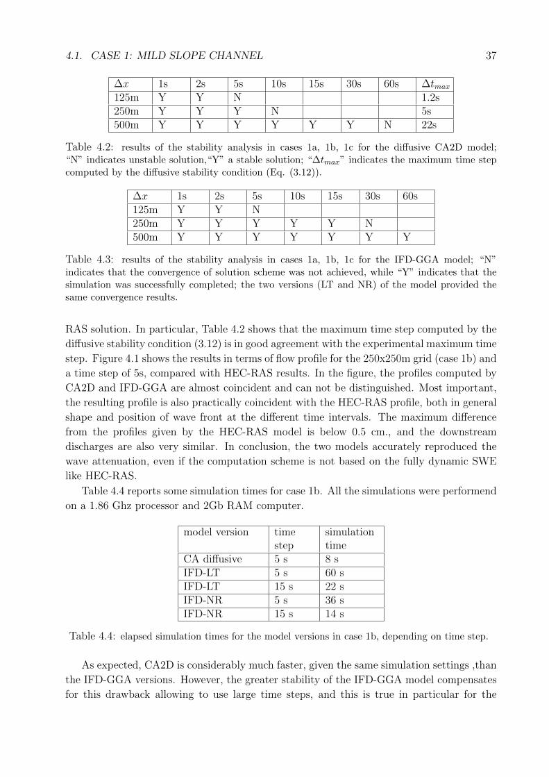
4.1. CASE 1: MILD SLOPE CHANNEL 37
∆x 1s 2s 5s 10s 15s 30s 60s ∆tmax125m Y Y N 1.2s250m Y Y Y N 5s500m Y Y Y Y Y Y N 22s
Table 4.2: results of the stability analysis in cases 1a, 1b, 1c for the diffusive CA2D model;“N” indicates unstable solution,“Y” a stable solution; “∆tmax” indicates the maximum time stepcomputed by the diffusive stability condition (Eq. (3.12)).
∆x 1s 2s 5s 10s 15s 30s 60s125m Y Y N250m Y Y Y Y Y N500m Y Y Y Y Y Y Y
Table 4.3: results of the stability analysis in cases 1a, 1b, 1c for the IFD-GGA model; “N”indicates that the convergence of solution scheme was not achieved, while “Y” indicates that thesimulation was successfully completed; the two versions (LT and NR) of the model provided thesame convergence results.
RAS solution. In particular, Table 4.2 shows that the maximum time step computed by the
diffusive stability condition (3.12) is in good agreement with the experimental maximum time
step. Figure 4.1 shows the results in terms of flow profile for the 250x250m grid (case 1b) and
a time step of 5s, compared with HEC-RAS results. In the figure, the profiles computed by
CA2D and IFD-GGA are almost coincident and can not be distinguished. Most important,
the resulting profile is also practically coincident with the HEC-RAS profile, both in general
shape and position of wave front at the different time intervals. The maximum difference
from the profiles given by the HEC-RAS model is below 0.5 cm., and the downstream
discharges are also very similar. In conclusion, the two models accurately reproduced the
wave attenuation, even if the computation scheme is not based on the fully dynamic SWE
like HEC-RAS.
Table 4.4 reports some simulation times for case 1b. All the simulations were performend
on a 1.86 Ghz processor and 2Gb RAM computer.
model version timestep
simulationtime
CA diffusive 5 s 8 sIFD-LT 5 s 60 sIFD-LT 15 s 22 sIFD-NR 5 s 36 sIFD-NR 15 s 14 s
Table 4.4: elapsed simulation times for the model versions in case 1b, depending on time step.
As expected, CA2D is considerably much faster, given the same simulation settings ,than
the IFD-GGA versions. However, the greater stability of the IFD-GGA model compensates
for this drawback allowing to use large time steps, and this is true in particular for the
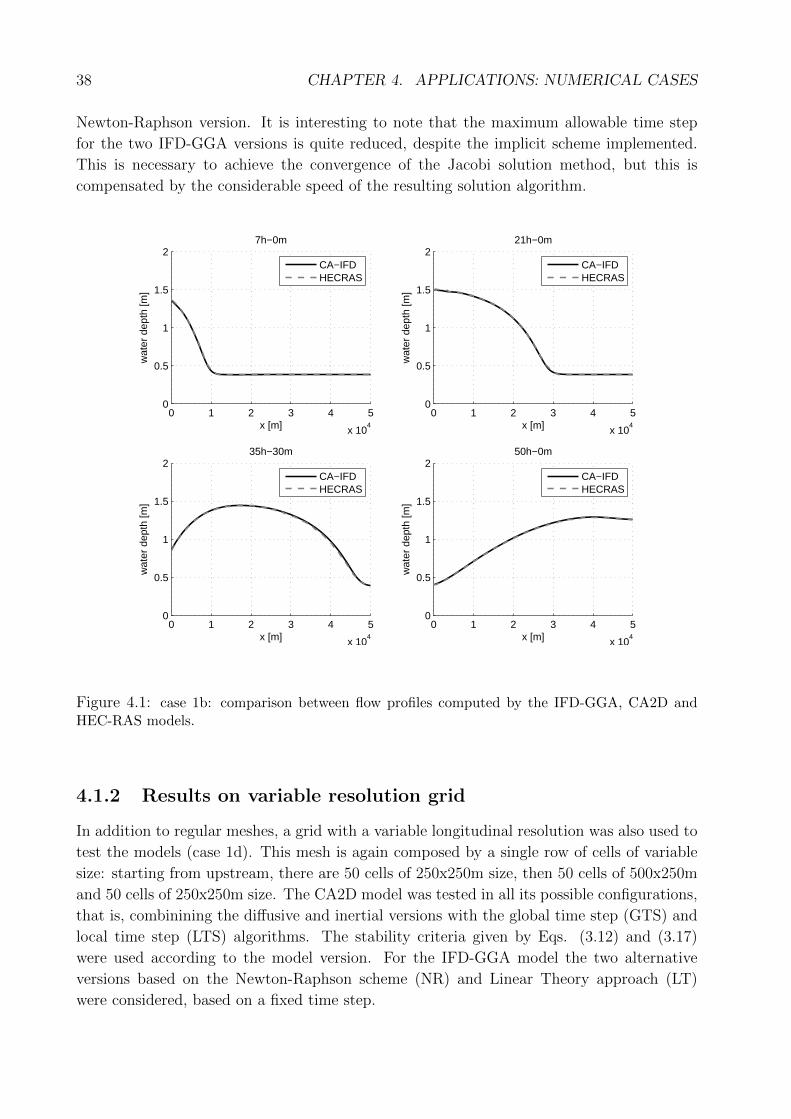
38 CHAPTER 4. APPLICATIONS: NUMERICAL CASES
Newton-Raphson version. It is interesting to note that the maximum allowable time step
for the two IFD-GGA versions is quite reduced, despite the implicit scheme implemented.
This is necessary to achieve the convergence of the Jacobi solution method, but this is
compensated by the considerable speed of the resulting solution algorithm.
0 1 2 3 4 5
x 104
0
0.5
1
1.5
2
wat
er d
epth
[m]
x [m]
7h−0m
CA−IFDHECRAS
0 1 2 3 4 5
x 104
0
0.5
1
1.5
2
wat
er d
epth
[m]
x [m]
21h−0m
CA−IFDHECRAS
0 1 2 3 4 5
x 104
0
0.5
1
1.5
2
wat
er d
epth
[m]
x [m]
35h−30m
CA−IFDHECRAS
0 1 2 3 4 5
x 104
0
0.5
1
1.5
2
wat
er d
epth
[m]
x [m]
50h−0m
CA−IFDHECRAS
Figure 4.1: case 1b: comparison between flow profiles computed by the IFD-GGA, CA2D andHEC-RAS models.
4.1.2 Results on variable resolution grid
In addition to regular meshes, a grid with a variable longitudinal resolution was also used to
test the models (case 1d). This mesh is again composed by a single row of cells of variable
size: starting from upstream, there are 50 cells of 250x250m size, then 50 cells of 500x250m
and 50 cells of 250x250m size. The CA2D model was tested in all its possible configurations,
that is, combinining the diffusive and inertial versions with the global time step (GTS) and
local time step (LTS) algorithms. The stability criteria given by Eqs. (3.12) and (3.17)
were used according to the model version. For the IFD-GGA model the two alternative
versions based on the Newton-Raphson scheme (NR) and Linear Theory approach (LT)
were considered, based on a fixed time step.
4.2. CASE 2: HILLSLOPE 39
As for the simulations with regular mesh, the profiles computed by all the different
versions of the models were practically coincident (as in Figure 4.1); again, the results were
also coincident with those of the the HEC-RAS model, with a maximum difference below
0.5 cm.
In Table 4.4 a comparison of overall simulation times is presented for case 1d. The
simulations were performed on a 1.86 Ghz Intel Core2 processor with 0.98Gb of RAM. For
the CA2D model, time steps provided by the stability conditions were found to correspond
to the experimental maximum values. For the CA2D inertial version, the CFL condition
with a 0.6 correction coefficient could be used. For the IFD-GGA versions, simulation times
with the maximum allowable time step are reported.
CA-GTSdiffusive
CA- LTSdiffusive
CA-GTSinertial
CA-LTSinertial
IFD-NR(∆t 15s)
IFD-LT(∆t 15s)
14 s 9 s 3 s 1 s 24s 41s
Table 4.5: case 1d: elapsed simulation times for the different model versions.
Focusing on Table 4.5, it can be seen how the inertial formulation produces considerable
improvement of CA2D model performance, in terms of reduction of computation times. The
advantage given by the LTS algorithm is significant but not as important. On the contrary,
computation times of the IFD-GGA versions are much larger.
4.2 Case 2: hillslope
This numerical case schematizes the overland flow produced by a rainfall over a hillslope,
and it has been presented by Di Giammarco et al. (1996). The hillslope is represented by an
inclined plane, which geometry is shown in Figure 4.2 and resumed in Table 4.6. The plane
has a 5% slope in the x direction and null slope in the y direction; this means that the plane
is equivalent to a series of one-dimensional parallel channels heading in the slope direction.
plane width 800 mplane length 1000 m
Manning roughness 0.015 m1/3sslope 0.05
Table 4.6: geometry and simulation settings of case 2.
The plane is initially dry; when the simulation begins, a rainfall with a constant intensity
in time and space of 10,8 mm/h is applied over all the plane; the rainfall has a 90min duration
and the simulation is run for a total time of 3h, to reproduce the draining of the simulation
area. A critical flow condition is imposed at the downstream boundary of the grid.
Although case 2 is in practice one-dimensional, it offers a good benchmark for a 2D
model for different reasons: first of all, an analytical solution for the outflow can be derived
from the kinematic wave equation, under the condition of semi-infinite plane. Secondly, the
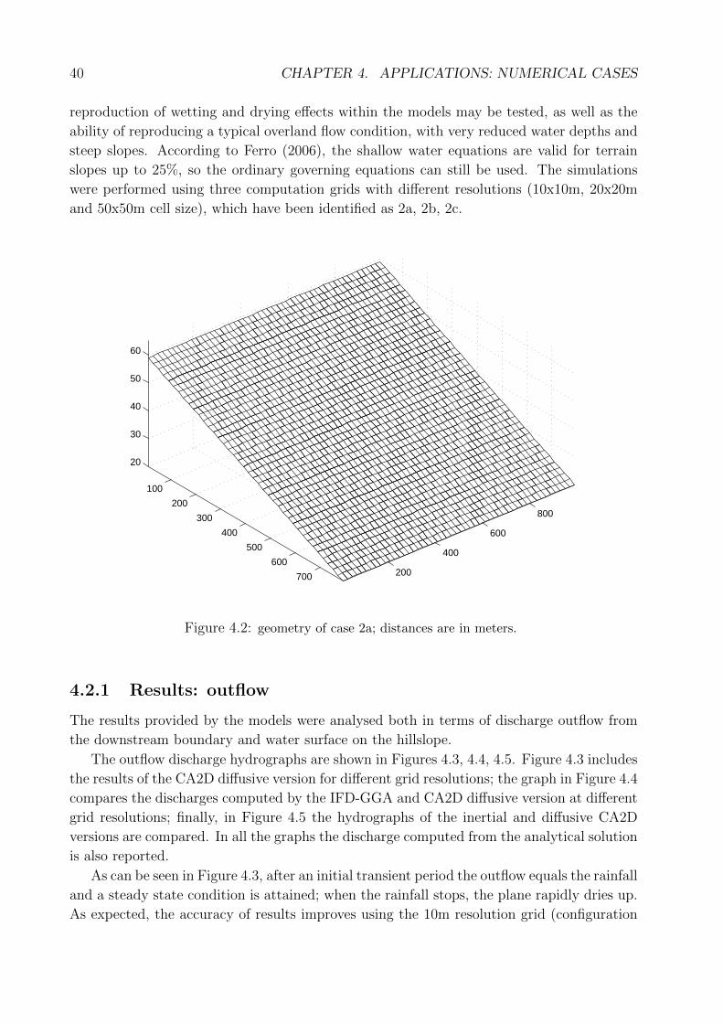
40 CHAPTER 4. APPLICATIONS: NUMERICAL CASES
reproduction of wetting and drying effects within the models may be tested, as well as the
ability of reproducing a typical overland flow condition, with very reduced water depths and
steep slopes. According to Ferro (2006), the shallow water equations are valid for terrain
slopes up to 25%, so the ordinary governing equations can still be used. The simulations
were performed using three computation grids with different resolutions (10x10m, 20x20m
and 50x50m cell size), which have been identified as 2a, 2b, 2c.
100
200
300
400
500
600
700 200
400
600
800
20
30
40
50
60
Figure 4.2: geometry of case 2a; distances are in meters.
4.2.1 Results: outflow
The results provided by the models were analysed both in terms of discharge outflow from
the downstream boundary and water surface on the hillslope.
The outflow discharge hydrographs are shown in Figures 4.3, 4.4, 4.5. Figure 4.3 includes
the results of the CA2D diffusive version for different grid resolutions; the graph in Figure 4.4
compares the discharges computed by the IFD-GGA and CA2D diffusive version at different
grid resolutions; finally, in Figure 4.5 the hydrographs of the inertial and diffusive CA2D
versions are compared. In all the graphs the discharge computed from the analytical solution
is also reported.
As can be seen in Figure 4.3, after an initial transient period the outflow equals the rainfall
and a steady state condition is attained; when the rainfall stops, the plane rapidly dries up.
As expected, the accuracy of results improves using the 10m resolution grid (configuration

4.2. CASE 2: HILLSLOPE 41
0 20 40 60 80 100 120 140 160 1800
0.5
1
1.5
2
2.5
disc
harg
e [m
3 /s]
time [min]
CA Δx 10mCA Δx 20mCA Δx 50manalytical
Figure 4.3: outflow computed by the analytical solution and the CA2D diffusive version at differentgrid resolutions
2a). Good results are obtained also with the 20m grid, while with the 50m grid a delay in the
hydrograph is observed, although the differences with the analytical solution are reduced.
It is worth noting that the drying phase is always well reproduced and does not instabilize
the model.
Similar comments can be made also for the results of the IFD-GGA versions, although
with sligth diferences with respect to CA2D diffusive model. As can be seen in Figure 4.4, the
outflow computed by the two models matches well the analytic solution when the 10m and
20m grids are used (although only the IFD-LT version could finish the simulation with the
10m resolution, as reported in Table 4.8). The performance of the IFD-GGA model is better
on the 50m grid. For the 20m and 50m resolution, the IFD-LT and IFD-NR configurations
provided almost the same results. Finally, the inertial CA2D version produces a slight
decrease in model accuracy (Figure 4.5).
4.2.2 Results: water surface profile
The analysis of water surface profiles gives provides interesting discussion points, as can
be seen in Figure 4.6. Despite the good reproduction of the total discharge, the CA2D
diffusive version has problems in reproducing the water surface, as along the flow direction
small oscillations appear, with alternate rows of “full” and “empty” cells where the actual
water depth is very low (below 0.1mm). It must be noted that such oscillations are not a
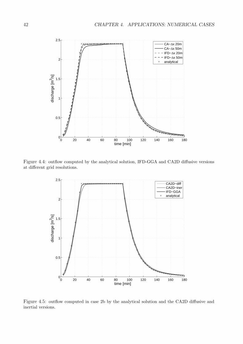
42 CHAPTER 4. APPLICATIONS: NUMERICAL CASES
0 20 40 60 80 100 120 140 160 1800
0.5
1
1.5
2
2.5
disc
harg
e [m
3 /s]
time [min]
CA−Δx 20mCA−Δx 50mIFD−Δx 20mIFD−Δx 50manalytical
Figure 4.4: outflow computed by the analytical solution, IFD-GGA and CA2D diffusive versionsat different grid resolutions.
0 20 40 60 80 100 120 140 160 1800
0.5
1
1.5
2
2.5
disc
harg
e [m
3 /s]
time [min]
CA2D−diffCA2D−inerIFD−GGAanalytical
Figure 4.5: outflow computed in case 2b by the analytical solution and the CA2D diffusive andinertial versions.
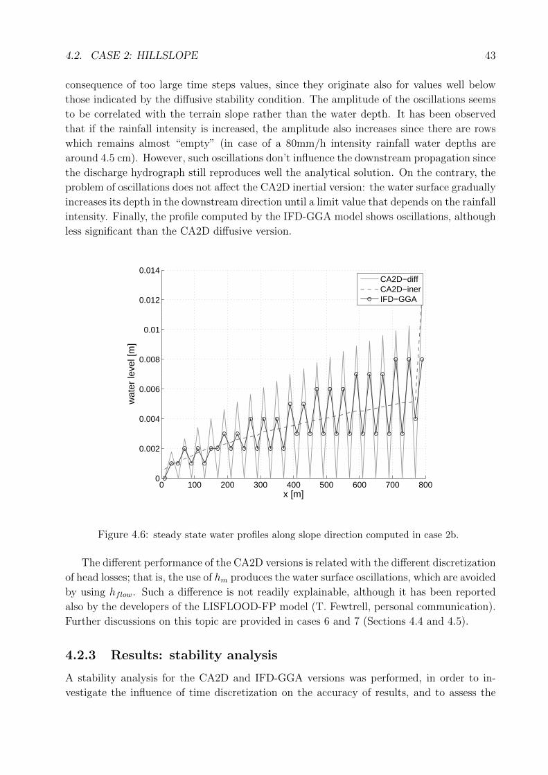
4.2. CASE 2: HILLSLOPE 43
consequence of too large time steps values, since they originate also for values well below
those indicated by the diffusive stability condition. The amplitude of the oscillations seems
to be correlated with the terrain slope rather than the water depth. It has been observed
that if the rainfall intensity is increased, the amplitude also increases since there are rows
which remains almost “empty” (in case of a 80mm/h intensity rainfall water depths are
around 4.5 cm). However, such oscillations don’t influence the downstream propagation since
the discharge hydrograph still reproduces well the analytical solution. On the contrary, the
problem of oscillations does not affect the CA2D inertial version: the water surface gradually
increases its depth in the downstream direction until a limit value that depends on the rainfall
intensity. Finally, the profile computed by the IFD-GGA model shows oscillations, although
less significant than the CA2D diffusive version.
0 100 200 300 400 500 600 700 8000
0.002
0.004
0.006
0.008
0.01
0.012
0.014
wat
er le
vel [
m]
x [m]
CA2D−diffCA2D−inerIFD−GGA
Figure 4.6: steady state water profiles along slope direction computed in case 2b.
The different performance of the CA2D versions is related with the different discretization
of head losses; that is, the use of hm produces the water surface oscillations, which are avoided
by using hflow. Such a difference is not readily explainable, although it has been reported
also by the developers of the LISFLOOD-FP model (T. Fewtrell, personal communication).
Further discussions on this topic are provided in cases 6 and 7 (Sections 4.4 and 4.5).
4.2.3 Results: stability analysis
A stability analysis for the CA2D and IFD-GGA versions was performed, in order to in-
vestigate the influence of time discretization on the accuracy of results, and to assess the
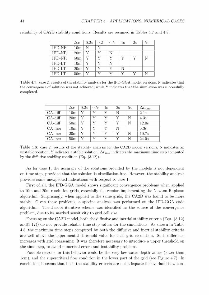
44 CHAPTER 4. APPLICATIONS: NUMERICAL CASES
reliability of CA2D stability conditions. Results are resumed in Tables 4.7 and 4.8.
∆x 0.2s 0.2s 0.5s 1s 2s 5sIFD-NR 10m N NIFD-NR 20m Y Y NIFD-NR 50m Y Y Y Y Y NIFD-LT 10m Y Y NIFD-LT 20m Y Y Y NIFD-LT 50m Y Y Y Y Y N
Table 4.7: case 2: results of the stability analysis for the IFD-GGA model versions; N indicates thatthe convergence of solution was not achieved, while Y indicates that the simulation was successfullycompleted.
∆x 0.2s 0.5s 1s 2s 5s ∆tmaxCA-diff 10m Y Y Y N 2.1sCA-diff 20m Y Y Y Y N 4.3sCA-diff 50m Y Y Y Y N 12.0sCA-iner 10m Y Y Y N 5.3sCA-iner 20m Y Y Y Y N 10.7sCA-iner 50m Y Y Y Y N 24.0s
Table 4.8: case 2: results of the stability analysis for the CA2D model versions; N indicates anunstable solution, Y indicates a stable solution; ∆tmax indicates the maximum time step computedby the diffusive stability condition (Eq. (3.12)).
As for case 1, the accuracy of the solutions provided by the models is not dependent
on time step, provided that the solution is obscillation-free. However, the stability analysis
provides some unexpected indications with respect to case 1.
First of all, the IFD-GGA model shows significant convergence problems when applied
to 10m and 20m resolution grids, especially the version implementing the Newton-Raphson
algorithm. Surprisingly, when applied to the same grids, the CA2D was found to be more
stable. Given these problems, a specific analysis was performed on the IFD-GGA code
algorithm. The Jacobi iterative scheme was identified as the source of the convergence
problem, due to its marked sensitivity to grid cell size.
Focusing on the CA2D model, both the diffusive and inertial stability criteria (Eqs. (3.12)
and(3.17)) do not provide reliable time step values for the simulations. As shown in Table
4.8, the maximum time steps computed by both the diffusive and inertial stability criteria
are well above the experimental threshold value for each grid resolution. Such difference
increases with grid coarsening. It was therefore necessary to introduce a upper threshold on
the time step, to avoid numerical errors and instability problems.
Possible reasons for this behavior could be the very low water depth values (lower than
1cm), and the supercritical flow condition in the lower part of the grid (see Figure 4.7). In
conclusion, it seems that both the stability criteria are not adequate for overland flow con-
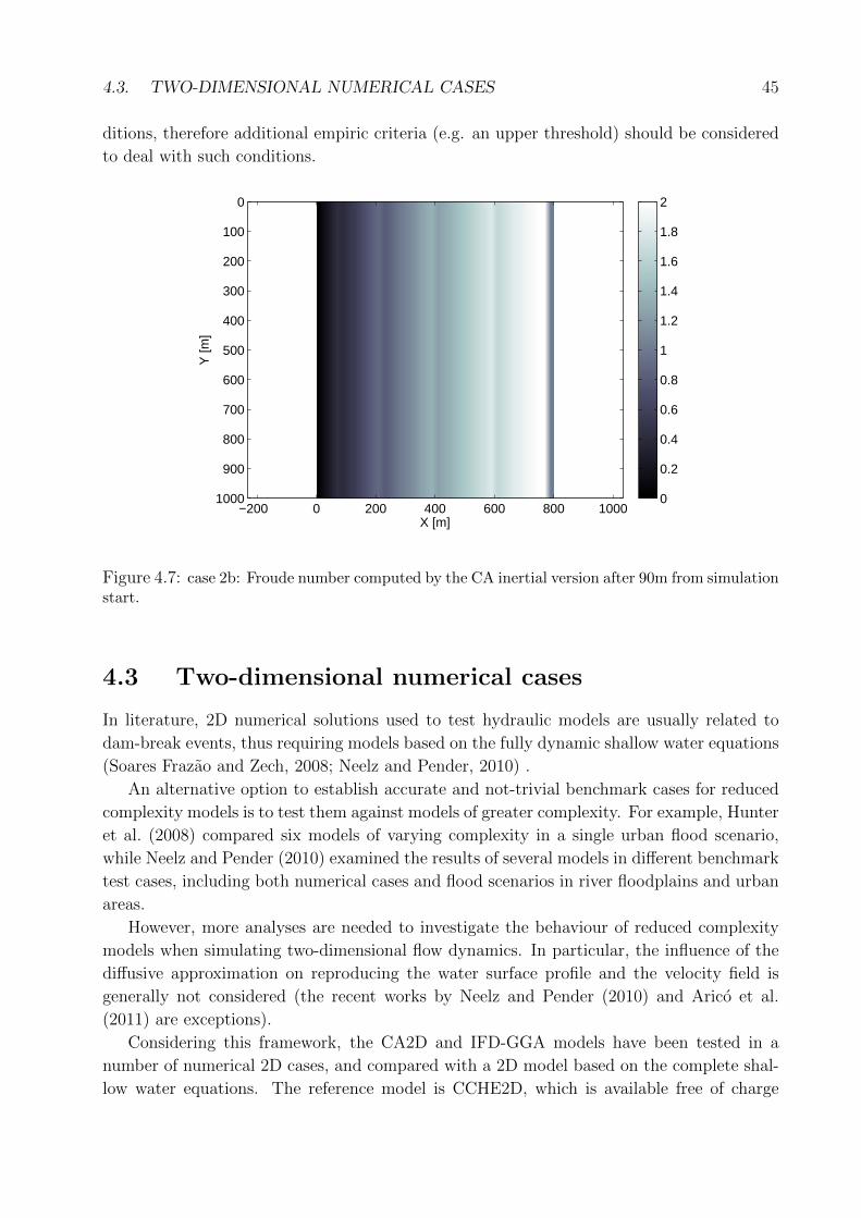
4.3. TWO-DIMENSIONAL NUMERICAL CASES 45
ditions, therefore additional empiric criteria (e.g. an upper threshold) should be considered
to deal with such conditions.
X [m]
Y [m
]
−200 0 200 400 600 800 1000
0
100
200
300
400
500
600
700
800
900
1000 0
0.2
0.4
0.6
0.8
1
1.2
1.4
1.6
1.8
2
Figure 4.7: case 2b: Froude number computed by the CA inertial version after 90m from simulationstart.
4.3 Two-dimensional numerical cases
In literature, 2D numerical solutions used to test hydraulic models are usually related to
dam-break events, thus requiring models based on the fully dynamic shallow water equations
(Soares Frazao and Zech, 2008; Neelz and Pender, 2010) .
An alternative option to establish accurate and not-trivial benchmark cases for reduced
complexity models is to test them against models of greater complexity. For example, Hunter
et al. (2008) compared six models of varying complexity in a single urban flood scenario,
while Neelz and Pender (2010) examined the results of several models in different benchmark
test cases, including both numerical cases and flood scenarios in river floodplains and urban
areas.
However, more analyses are needed to investigate the behaviour of reduced complexity
models when simulating two-dimensional flow dynamics. In particular, the influence of the
diffusive approximation on reproducing the water surface profile and the velocity field is
generally not considered (the recent works by Neelz and Pender (2010) and Arico et al.
(2011) are exceptions).
Considering this framework, the CA2D and IFD-GGA models have been tested in a
number of numerical 2D cases, and compared with a 2D model based on the complete shal-
low water equations. The reference model is CCHE2D, which is available free of charge
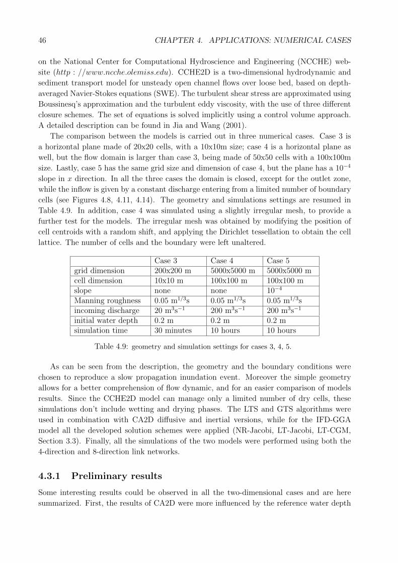
46 CHAPTER 4. APPLICATIONS: NUMERICAL CASES
on the National Center for Computational Hydroscience and Engineering (NCCHE) web-
site (http : //www.ncche.olemiss.edu). CCHE2D is a two-dimensional hydrodynamic and
sediment transport model for unsteady open channel flows over loose bed, based on depth-
averaged Navier-Stokes equations (SWE). The turbulent shear stress are approximated using
Boussinesq’s approximation and the turbulent eddy viscosity, with the use of three different
closure schemes. The set of equations is solved implicitly using a control volume approach.
A detailed description can be found in Jia and Wang (2001).
The comparison between the models is carried out in three numerical cases. Case 3 is
a horizontal plane made of 20x20 cells, with a 10x10m size; case 4 is a horizontal plane as
well, but the flow domain is larger than case 3, being made of 50x50 cells with a 100x100m
size. Lastly, case 5 has the same grid size and dimension of case 4, but the plane has a 10−4
slope in x direction. In all the three cases the domain is closed, except for the outlet zone,
while the inflow is given by a constant discharge entering from a limited number of boundary
cells (see Figures 4.8, 4.11, 4.14). The geometry and simulations settings are resumed in
Table 4.9. In addition, case 4 was simulated using a slightly irregular mesh, to provide a
further test for the models. The irregular mesh was obtained by modifying the position of
cell centroids with a random shift, and applying the Dirichlet tessellation to obtain the cell
lattice. The number of cells and the boundary were left unaltered.
Case 3 Case 4 Case 5grid dimension 200x200 m 5000x5000 m 5000x5000 mcell dimension 10x10 m 100x100 m 100x100 mslope none none 10−4
Manning roughness 0.05 m1/3s 0.05 m1/3s 0.05 m1/3sincoming discharge 20 m3s−1 200 m3s−1 200 m3s−1
initial water depth 0.2 m 0.2 m 0.2 msimulation time 30 minutes 10 hours 10 hours
Table 4.9: geometry and simulation settings for cases 3, 4, 5.
As can be seen from the description, the geometry and the boundary conditions were
chosen to reproduce a slow propagation inundation event. Moreover the simple geometry
allows for a better comprehension of flow dynamic, and for an easier comparison of models
results. Since the CCHE2D model can manage only a limited number of dry cells, these
simulations don’t include wetting and drying phases. The LTS and GTS algorithms were
used in combination with CA2D diffusive and inertial versions, while for the IFD-GGA
model all the developed solution schemes were applied (NR-Jacobi, LT-Jacobi, LT-CGM,
Section 3.3). Finally, all the simulations of the two models were performed using both the
4-direction and 8-direction link networks.
4.3.1 Preliminary results
Some interesting results could be observed in all the two-dimensional cases and are here
summarized. First, the results of CA2D were more influenced by the reference water depth
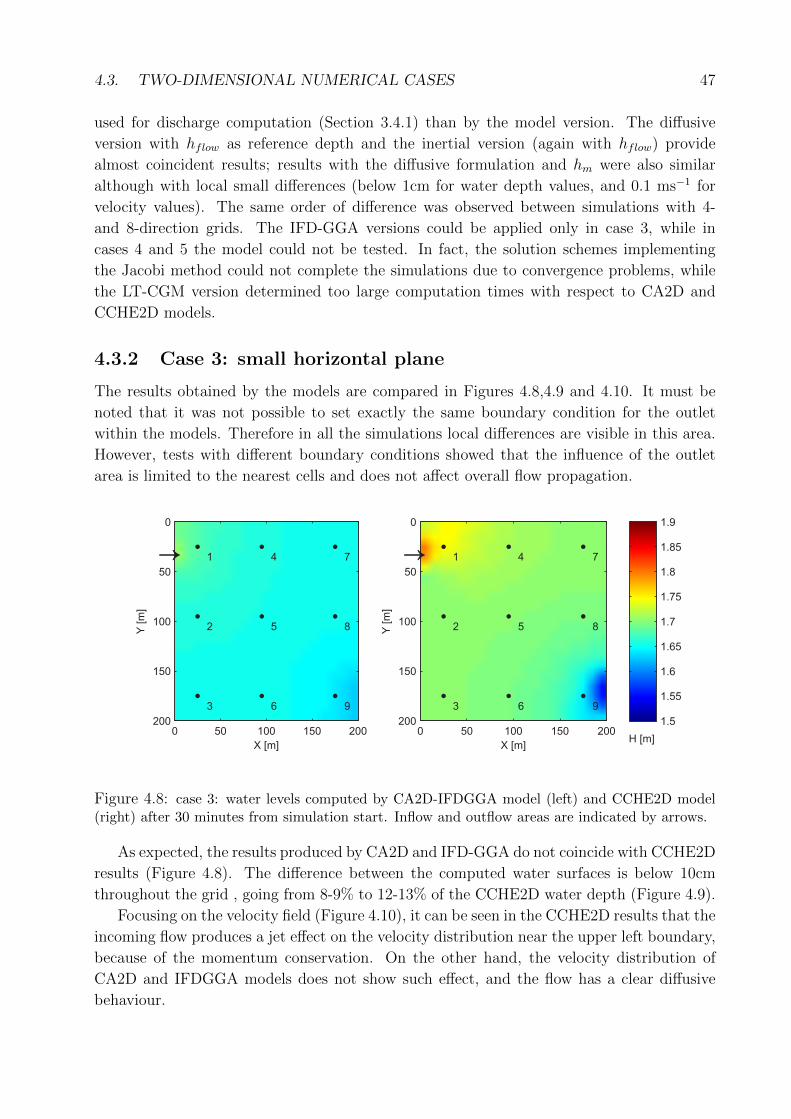
4.3. TWO-DIMENSIONAL NUMERICAL CASES 47
used for discharge computation (Section 3.4.1) than by the model version. The diffusive
version with hflow as reference depth and the inertial version (again with hflow) provide
almost coincident results; results with the diffusive formulation and hm were also similar
although with local small differences (below 1cm for water depth values, and 0.1 ms−1 for
velocity values). The same order of difference was observed between simulations with 4-
and 8-direction grids. The IFD-GGA versions could be applied only in case 3, while in
cases 4 and 5 the model could not be tested. In fact, the solution schemes implementing
the Jacobi method could not complete the simulations due to convergence problems, while
the LT-CGM version determined too large computation times with respect to CA2D and
CCHE2D models.
4.3.2 Case 3: small horizontal plane
The results obtained by the models are compared in Figures 4.8,4.9 and 4.10. It must be
noted that it was not possible to set exactly the same boundary condition for the outlet
within the models. Therefore in all the simulations local differences are visible in this area.
However, tests with different boundary conditions showed that the influence of the outlet
area is limited to the nearest cells and does not affect overall flow propagation.
X [m]
Y[m
]
1
2
3
4
5
6
7
8
9
→
0 50 100 150 200
0
50
100
150
200
X [m]
Y[m
]
1
2
3
4
5
6
7
8
9
→
0 50 100 150 200
0
50
100
150
200 1.5
1.55
1.6
1.65
1.7
1.75
1.8
1.85
1.9
H [m]
Figure 4.8: case 3: water levels computed by CA2D-IFDGGA model (left) and CCHE2D model(right) after 30 minutes from simulation start. Inflow and outflow areas are indicated by arrows.
As expected, the results produced by CA2D and IFD-GGA do not coincide with CCHE2D
results (Figure 4.8). The difference between the computed water surfaces is below 10cm
throughout the grid , going from 8-9% to 12-13% of the CCHE2D water depth (Figure 4.9).
Focusing on the velocity field (Figure 4.10), it can be seen in the CCHE2D results that the
incoming flow produces a jet effect on the velocity distribution near the upper left boundary,
because of the momentum conservation. On the other hand, the velocity distribution of
CA2D and IFDGGA models does not show such effect, and the flow has a clear diffusive
behaviour.
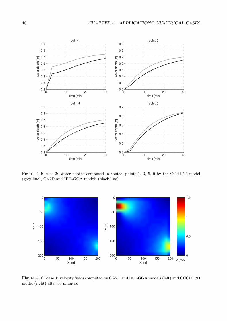
48 CHAPTER 4. APPLICATIONS: NUMERICAL CASES
0 10 20 300.2
0.3
0.4
0.5
0.6
0.7
0.8
0.9
wate
rdepth
[m]
time [min]
point-1
0 10 20 300.2
0.3
0.4
0.5
0.6
0.7
0.8
0.9
wate
rdepth
[m]
time [min]
point-3
0 10 20 300.2
0.3
0.4
0.5
0.6
0.7
0.8
0.9
wate
rdepth
[m]
time [min]
point-5
0 10 20 300.2
0.3
0.4
0.5
0.6
0.7
wate
rdepth
[m]
time [min]
point-9
Figure 4.9: case 3: water depths computed in control points 1, 3, 5, 9 by the CCHE2D model(grey line), CA2D and IFD-GGA models (black line).
X [m]
Y[m
]
0 50 100 150 200
0
50
100
150
200
X [m]
Y[m
]
0 50 100 150 200
0
50
100
150
200 0
0.5
1
1.5
V [m/s]
Figure 4.10: case 3: velocity fields computed by CA2D and IFD-GGA models (left) and CCCHE2Dmodel (right) after 30 minutes.
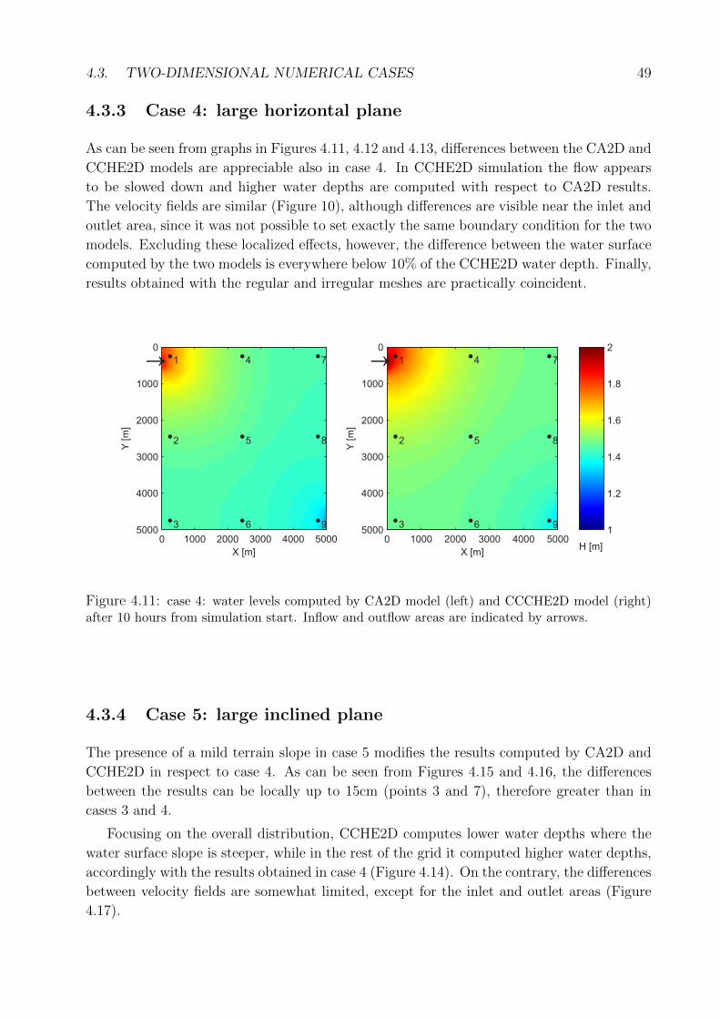
4.3. TWO-DIMENSIONAL NUMERICAL CASES 49
4.3.3 Case 4: large horizontal plane
As can be seen from graphs in Figures 4.11, 4.12 and 4.13, differences between the CA2D and
CCHE2D models are appreciable also in case 4. In CCHE2D simulation the flow appears
to be slowed down and higher water depths are computed with respect to CA2D results.
The velocity fields are similar (Figure 10), although differences are visible near the inlet and
outlet area, since it was not possible to set exactly the same boundary condition for the two
models. Excluding these localized effects, however, the difference between the water surface
computed by the two models is everywhere below 10% of the CCHE2D water depth. Finally,
results obtained with the regular and irregular meshes are practically coincident.
X [m]
Y[m
]
1
2
3
4
5
6
7
8
9
→
0 1000 2000 3000 4000 5000
0
1000
2000
3000
4000
5000
X [m]
Y[m
]1
2
3
4
5
6
7
8
9
→
0 1000 2000 3000 4000 5000
0
1000
2000
3000
4000
5000 1
1.2
1.4
1.6
1.8
2
H [m]
Figure 4.11: case 4: water levels computed by CA2D model (left) and CCCHE2D model (right)after 10 hours from simulation start. Inflow and outflow areas are indicated by arrows.
4.3.4 Case 5: large inclined plane
The presence of a mild terrain slope in case 5 modifies the results computed by CA2D and
CCHE2D in respect to case 4. As can be seen from Figures 4.15 and 4.16, the differences
between the results can be locally up to 15cm (points 3 and 7), therefore greater than in
cases 3 and 4.
Focusing on the overall distribution, CCHE2D computes lower water depths where the
water surface slope is steeper, while in the rest of the grid it computed higher water depths,
accordingly with the results obtained in case 4 (Figure 4.14). On the contrary, the differences
between velocity fields are somewhat limited, except for the inlet and outlet areas (Figure
4.17).
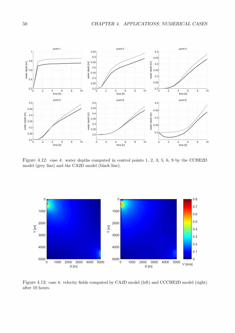
50 CHAPTER 4. APPLICATIONS: NUMERICAL CASES
0 2 4 6 8 100.2
0.4
0.6
0.8
1
wate
rdep
th[m
]
time [h]
point-1
0 2 4 6 8 100.2
0.25
0.3
0.35
0.4
0.45
0.5
0.55
wate
rdep
th[m
]
time [h]
point-2
0 2 4 6 8 100.2
0.25
0.3
0.35
0.4
0.45
0.5
wate
rdepth
[m]
time [h]
point-3
0 2 4 6 8 100.2
0.25
0.3
0.35
0.4
0.45
0.5
wate
rdepth
[m]
time [h]
point-5
Figure 4.12: case 4: water depths computed in control points 1, 2, 3, 5, 6, 9 by the CCHE2Dmodel (grey line) and the CA2D model (black line).
X [m]
Y[m
]
0 1000 2000 3000 4000 5000
0
1000
2000
3000
4000
5000
X [m]
Y[m
]
0 1000 2000 3000 4000 5000
0
1000
2000
3000
4000
5000 0
0.1
0.2
0.3
0.4
0.5
0.6
0.7
0.8
V [m/s]
Figure 4.13: case 4: velocity fields computed by CA2D model (left) and CCCHE2D model (right)after 10 hours.
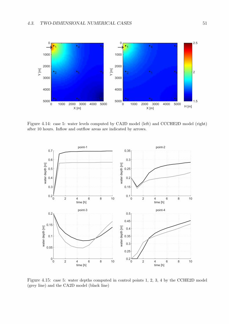
4.3. TWO-DIMENSIONAL NUMERICAL CASES 51
X [m]
Y[m
]
1
2
3
4
5
6
7
8
9
→
0 1000 2000 3000 4000 5000
0
1000
2000
3000
4000
5000
X [m]Y
[m]
1
2
3
4
5
6
7
8
9
→
0 1000 2000 3000 4000 5000
0
1000
2000
3000
4000
5000 1.5
2
2.5
H [m]
Figure 4.14: case 5: water levels computed by CA2D model (left) and CCCHE2D model (right)after 10 hours. Inflow and outflow areas are indicated by arrows.
0 2 4 6 8 100.2
0.3
0.4
0.5
0.6
0.7
wate
rdepth
[m]
time [h]
point-1
0 2 4 6 8 100.1
0.15
0.2
0.25
0.3
0.35
wate
rdepth
[m]
time [h]
point-2
0 2 4 6 8 100
0.05
0.1
0.15
0.2
wate
rdepth
[m]
time [h]
point-3
0 2 4 6 8 100.2
0.25
0.3
0.35
0.4
0.45
0.5
wate
rdepth
[m]
time [h]
point-4
Figure 4.15: case 5: water depths computed in control points 1, 2, 3, 4 by the CCHE2D model(grey line) and the CA2D model (black line)
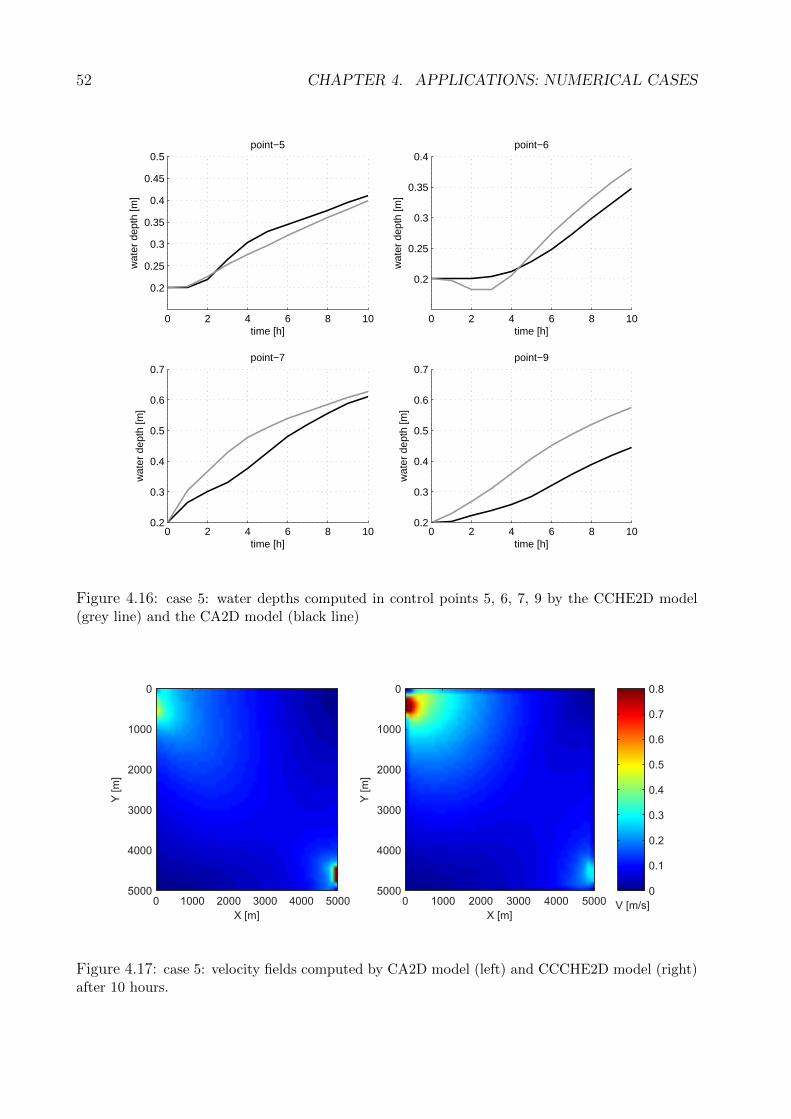
52 CHAPTER 4. APPLICATIONS: NUMERICAL CASES
0 2 4 6 8 10
0.2
0.25
0.3
0.35
0.4
0.45
0.5
wat
er d
epth
[m]
time [h]
point−5
0 2 4 6 8 10
0.2
0.25
0.3
0.35
0.4
wat
er d
epth
[m]
time [h]
point−6
0 2 4 6 8 100.2
0.3
0.4
0.5
0.6
0.7
wat
er d
epth
[m]
time [h]
point−7
0 2 4 6 8 100.2
0.3
0.4
0.5
0.6
0.7
wat
er d
epth
[m]
time [h]
point−9
Figure 4.16: case 5: water depths computed in control points 5, 6, 7, 9 by the CCHE2D model(grey line) and the CA2D model (black line)
X [m]
Y[m
]
0 1000 2000 3000 4000 5000
0
1000
2000
3000
4000
5000
X [m]
Y[m
]
0 1000 2000 3000 4000 5000
0
1000
2000
3000
4000
5000 0
0.1
0.2
0.3
0.4
0.5
0.6
0.7
0.8
V [m/s]
Figure 4.17: case 5: velocity fields computed by CA2D model (left) and CCCHE2D model (right)after 10 hours.
4.3. TWO-DIMENSIONAL NUMERICAL CASES 53
4.3.5 Discussion
Some considerations can be made about the observed results. Since the inertial and diffusive
versions of the CA2D model provided similar results, the differences in respect to CCHE2D
should be explained as an effect of advection terms of the momentum equation. This suggests
that the importance of advection terms is not negligible in 2D flow, even though further
numerical analyses are needed to investigate its magnitude in a wider range of flow conditions.
It is worth noting that the CA2D model maintained a diffusive behaviour also when
using the inertial formulation, as can be inferred from the results of case 3 (Figure 4.10).
This can be explained considering that in the model structure no information about the flow
direction is transferred between adjacent cells: the hydraulic head is stored in cells simply
as water level and flow components are decoupled. This schematization comes from the
diffusive approximation but is conserved also in the inertial formulation, due to the drop of
advection terms, so that momuntum conservation is still incomplete.
In conclusion, the introduction of the inertial term within the model is very effective for
stabilizing the flow along the connections, but it seems to add little further description of
flow dynamics, at least in the presented cases. Similar results were observed also by Bates
et al. (2010) in applying the inertial and diffusive versions of the LISFLOOD-FP model to
a urban flood scenario.
These observations can be used to draw some preliminary conclusions about the per-
formance of the diffusive approximation in the simulation of flood events. Further analyses
will be presented in Chapter 5.
Results obtained in case 3 indicate that the CA2D model can reproduce locally con-
centrated flows only with some approximation. Nevertheless, the overall results in cases
3,4,5 suggest that localized flow conditions may have a minor influence on overall 2D flood
propagation, as concluded by previous research studies (Hunter et al., 2008; Neelz and Pen-
der, 2010).
In particular, the observed differences between CA2D and CCHE2D are comparable
with the uncertainty normally associated to available “real world” data for flood events.
For example, according to Fewtrell et al. (2007) and Hunter et al. (2008), LiDAR data
have a typical vertical error of ±15 cm, comparable with the maximum difference in water
depths observed in case 5. High level of uncertainty are also associated with calibration and
evaluation data, like inundation extent maps from SAR imagery, or measurements of water
level from water marks (Horritt et al., 2007; Neal et al., 2009a).
4.3.6 Simulation times
Table 4.10 reports run times for the simulations performed with CCHE2D, IFD-GGA and
the CA2D models. All the simulations were run on a 1.25 Ghz Intel processor with 2.00 Gb
of RAM. The CCHE2D model uses an implicit time marching scheme with a constant time
step, so the maximum allowable values reported in Table 4.10 were chosen with a trial-and-
error procedure. As reported in Section 4.3.1, the IFD-GGA model could be run only in
case 3, while in cases 4 and 5 the model was too slow (run times exceeded two hours).
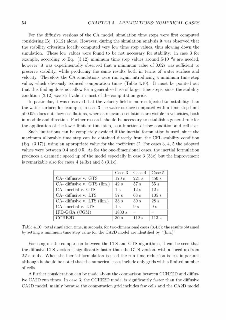
54 CHAPTER 4. APPLICATIONS: NUMERICAL CASES
For the diffusive versions of the CA model, simulation time steps were first computed
considering Eq. (3.12) alone. However, during the simulation analysis it was observed that
the stability criterium locally computed very low time step values, thus slowing down the
simulation. These low values were found to be not necessary for stability: in case 3 for
example, according to Eq. (3.12) minimum time step values around 5·10−3s are needed;
however, it was experimentally observed that a minimum value of 0.02s was sufficient to
preserve stability, while producing the same results both in terms of water surface and
velocity. Therefore the CA simulations were run again introducing a minimum time step
value, which obviously reduced computation times (Table 4.10). It must be pointed out
that this finding does not allow for a generalized use of larger time steps, since the stability
condition (3.12) was still valid in most of the computation grids.
In particular, it was observed that the velocity field is more subjected to instability than
the water surface; for example, in case 3 the water surface computed with a time step limit
of 0.05s does not show oscillations, whereas relevant oscillations are visible in velocities, both
in module and direction. Further research should be necessary to establish a general rule for
the application of the lower limit to time step, as a function of flow condition and cell size.
Such limitations can be completely avoided if the inertial formulation is used, since the
maximum allowable time step can be obtained directly from the CFL stability condition
(Eq. (3.17)), using an appropriate value for the coefficient C. For cases 3, 4, 5 the adopted
values were between 0.4 and 0.5. As for the one-dimensional cases, the inertial formulation
produces a dramatic speed up of the model especially in case 3 (33x) but the improvement
is remarkable also for cases 4 (4.3x) and 5 (3.1x).
Case 3 Case 4 Case 5CA- diffusive v. GTS 170 s 221 s 450 sCA- diffusive v. GTS (lim.) 42 s 57 s 55 sCA- inertial v. GTS 1 s 12 s 12 sCA- diffusive v. LTS 57 s 68 s 105 sCA- diffusive v. LTS (lim.) 33 s 39 s 28 sCA- inertial v. LTS 1 s 9 s 9 sIFD-GGA (CGM) 1800 s – –CCHE2D 30 s 112 s 113 s
Table 4.10: total simulation time, in seconds, for two-dimensional cases (3,4,5); the results obtainedby setting a minimum time step value for the CA2D model are identified by “(lim.)”
Focusing on the comparison between the LTS and GTS algorithms, it can be seen that
the diffusive LTS version is significantly faster than the GTS version, with a speed up from
2.5x to 4x. When the inertial formulation is used the run time reduction is less important
although it should be noted that the numerical cases include only grids with a limited number
of cells.
A further consideration can be made about the comparison between CCHE2D and diffus-
ive CA2D run times. In case 3, the CCHE2D model is significantly faster than the diffusive
CA2D model, mainly because the computation grid includes few cells and the CA2D model
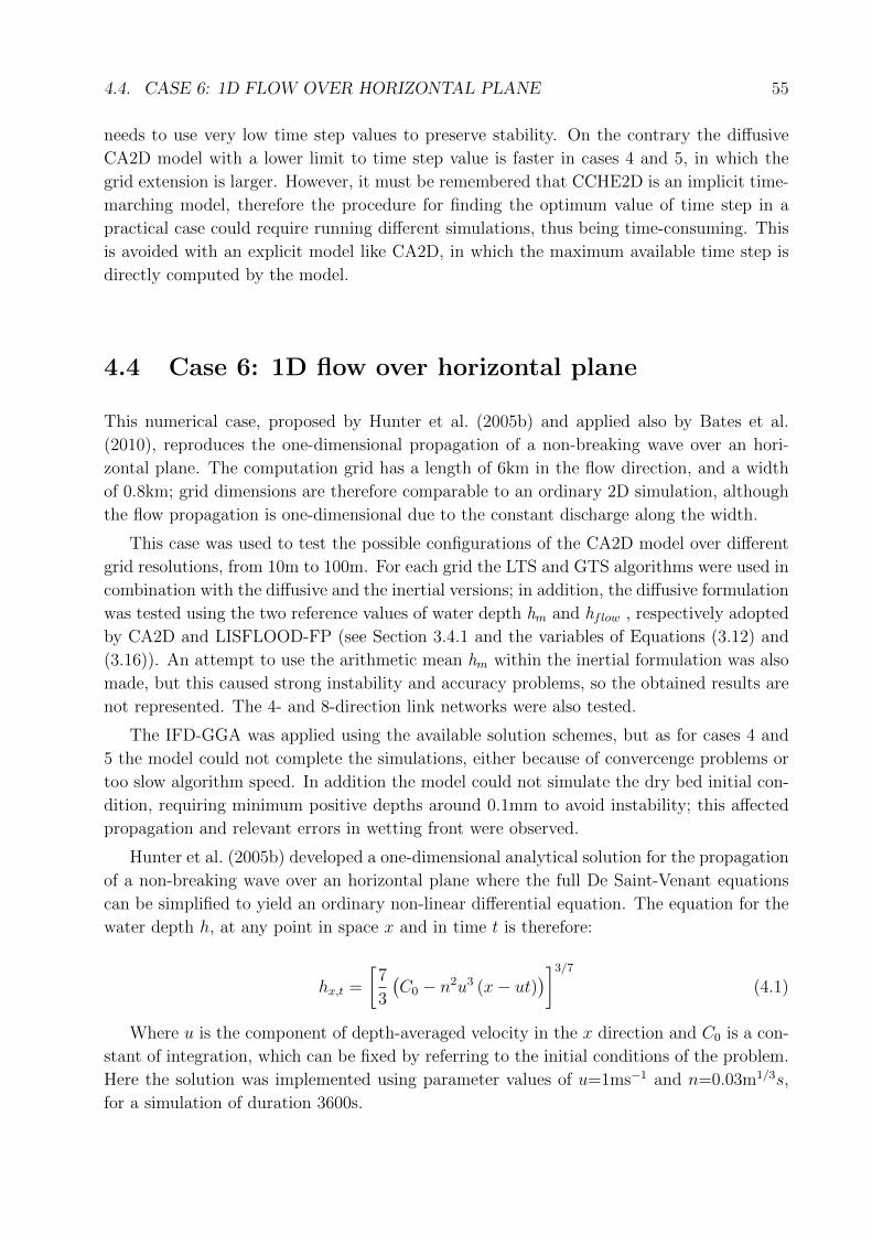
4.4. CASE 6: 1D FLOW OVER HORIZONTAL PLANE 55
needs to use very low time step values to preserve stability. On the contrary the diffusive
CA2D model with a lower limit to time step value is faster in cases 4 and 5, in which the
grid extension is larger. However, it must be remembered that CCHE2D is an implicit time-
marching model, therefore the procedure for finding the optimum value of time step in a
practical case could require running different simulations, thus being time-consuming. This
is avoided with an explicit model like CA2D, in which the maximum available time step is
directly computed by the model.
4.4 Case 6: 1D flow over horizontal plane
This numerical case, proposed by Hunter et al. (2005b) and applied also by Bates et al.
(2010), reproduces the one-dimensional propagation of a non-breaking wave over an hori-
zontal plane. The computation grid has a length of 6km in the flow direction, and a width
of 0.8km; grid dimensions are therefore comparable to an ordinary 2D simulation, although
the flow propagation is one-dimensional due to the constant discharge along the width.
This case was used to test the possible configurations of the CA2D model over different
grid resolutions, from 10m to 100m. For each grid the LTS and GTS algorithms were used in
combination with the diffusive and the inertial versions; in addition, the diffusive formulation
was tested using the two reference values of water depth hm and hflow , respectively adopted
by CA2D and LISFLOOD-FP (see Section 3.4.1 and the variables of Equations (3.12) and
(3.16)). An attempt to use the arithmetic mean hm within the inertial formulation was also
made, but this caused strong instability and accuracy problems, so the obtained results are
not represented. The 4- and 8-direction link networks were also tested.
The IFD-GGA was applied using the available solution schemes, but as for cases 4 and
5 the model could not complete the simulations, either because of convercenge problems or
too slow algorithm speed. In addition the model could not simulate the dry bed initial con-
dition, requiring minimum positive depths around 0.1mm to avoid instability; this affected
propagation and relevant errors in wetting front were observed.
Hunter et al. (2005b) developed a one-dimensional analytical solution for the propagation
of a non-breaking wave over an horizontal plane where the full De Saint-Venant equations
can be simplified to yield an ordinary non-linear differential equation. The equation for the
water depth h, at any point in space x and in time t is therefore:
hx,t =
[7
3
(C0 − n2u3 (x− ut)
)]3/7
(4.1)
Where u is the component of depth-averaged velocity in the x direction and C0 is a con-
stant of integration, which can be fixed by referring to the initial conditions of the problem.
Here the solution was implemented using parameter values of u=1ms−1 and n=0.03m1/3s,
for a simulation of duration 3600s.
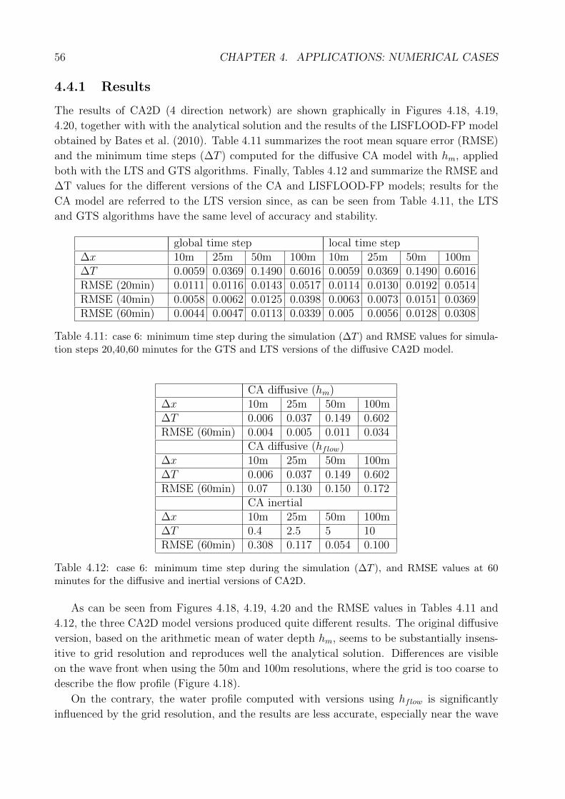
56 CHAPTER 4. APPLICATIONS: NUMERICAL CASES
4.4.1 Results
The results of CA2D (4 direction network) are shown graphically in Figures 4.18, 4.19,
4.20, together with with the analytical solution and the results of the LISFLOOD-FP model
obtained by Bates et al. (2010). Table 4.11 summarizes the root mean square error (RMSE)
and the minimum time steps (∆T ) computed for the diffusive CA model with hm, applied
both with the LTS and GTS algorithms. Finally, Tables 4.12 and summarize the RMSE and
∆T values for the different versions of the CA and LISFLOOD-FP models; results for the
CA model are referred to the LTS version since, as can be seen from Table 4.11, the LTS
and GTS algorithms have the same level of accuracy and stability.
global time step local time step∆x 10m 25m 50m 100m 10m 25m 50m 100m∆T 0.0059 0.0369 0.1490 0.6016 0.0059 0.0369 0.1490 0.6016RMSE (20min) 0.0111 0.0116 0.0143 0.0517 0.0114 0.0130 0.0192 0.0514RMSE (40min) 0.0058 0.0062 0.0125 0.0398 0.0063 0.0073 0.0151 0.0369RMSE (60min) 0.0044 0.0047 0.0113 0.0339 0.005 0.0056 0.0128 0.0308
Table 4.11: case 6: minimum time step during the simulation (∆T ) and RMSE values for simula-tion steps 20,40,60 minutes for the GTS and LTS versions of the diffusive CA2D model.
CA diffusive (hm)∆x 10m 25m 50m 100m∆T 0.006 0.037 0.149 0.602RMSE (60min) 0.004 0.005 0.011 0.034
CA diffusive (hflow)∆x 10m 25m 50m 100m∆T 0.006 0.037 0.149 0.602RMSE (60min) 0.07 0.130 0.150 0.172
CA inertial∆x 10m 25m 50m 100m∆T 0.4 2.5 5 10RMSE (60min) 0.308 0.117 0.054 0.100
Table 4.12: case 6: minimum time step during the simulation (∆T ), and RMSE values at 60minutes for the diffusive and inertial versions of CA2D.
As can be seen from Figures 4.18, 4.19, 4.20 and the RMSE values in Tables 4.11 and
4.12, the three CA2D model versions produced quite different results. The original diffusive
version, based on the arithmetic mean of water depth hm, seems to be substantially insens-
itive to grid resolution and reproduces well the analytical solution. Differences are visible
on the wave front when using the 50m and 100m resolutions, where the grid is too coarse to
describe the flow profile (Figure 4.18).
On the contrary, the water profile computed with versions using hflow is significantly
influenced by the grid resolution, and the results are less accurate, especially near the wave
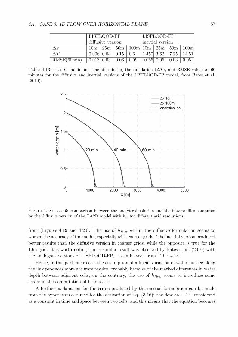
4.4. CASE 6: 1D FLOW OVER HORIZONTAL PLANE 57
LISFLOOD-FPdiffusive version
LISFLOOD-FPinertial version
∆x 10m 25m 50m 100m 10m 25m 50m 100m∆T 0.006 0.04 0.15 0.6 1.450 3.62 7.25 14.51RMSE(60min) 0.013 0.03 0.06 0.09 0.065 0.05 0.03 0.05
Table 4.13: case 6: minimum time step during the simulation (∆T ), and RMSE values at 60minutes for the diffusive and inertial versions of the LISFLOOD-FP model, from Bates et al.(2010).
0 1000 2000 3000 4000 50000
0.5
1
1.5
2
2.5
20 min 40 min 60 min
wate
rdepth
[m]
x [m]
∆x 10m.
∆x 100m
analytical sol.
Figure 4.18: case 6: comparison between the analytical solution and the flow profiles computedby the diffusive version of the CA2D model with hm for different grid resolutions.
front (Figures 4.19 and 4.20). The use of hflow within the diffusive formulation seems to
worsen the accuracy of the model, especially with coarser grids. The inertial version produced
better results than the diffusive version in coarser grids, while the opposite is true for the
10m grid. It is worth noting that a similar result was observed by Bates et al. (2010) with
the analogous versions of LISFLOOD-FP, as can be seen from Table 4.13.
Hence, in this particular case, the assumption of a linear variation of water surface along
the link produces more accurate results, probably because of the marked differences in water
depth between adjacent cells; on the contrary, the use of hflow seems to introduce some
errors in the computation of head losses.
A further explanation for the errors produced by the inertial formulation can be made
from the hypotheses assumed for the derivation of Eq. (3.16): the flow area A is considered
as a constant in time and space between two cells, and this means that the equation becomes
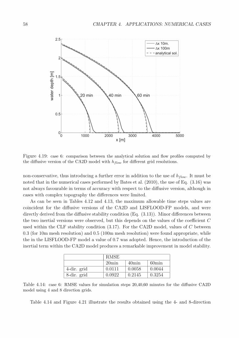
58 CHAPTER 4. APPLICATIONS: NUMERICAL CASES
0 1000 2000 3000 4000 50000
0.5
1
1.5
2
2.5
20 min 40 min 60 min
wate
rdepth
[m]
x [m]
∆x 10m.
∆x 100m
analytical sol.
Figure 4.19: case 6: comparison between the analytical solution and flow profiles computed bythe diffusive version of the CA2D model with hflow for different grid resolutions.
non-conservative, thus introducing a further error in addition to the use of hflow. It must be
noted that in the numerical cases performed by Bates et al. (2010), the use of Eq. (3.16) was
not always favourable in terms of accuracy with respect to the diffusive version, although in
cases with complex topography the differences were limited.
As can be seen in Tables 4.12 and 4.13, the maximum allowable time steps values are
coincident for the diffusive versions of the CA2D and LISFLOOD-FP models, and were
directly derived from the diffusive stability condition (Eq. (3.13)). Minor differences between
the two inertial versions were observed, but this depends on the values of the coefficient C
used within the CLF stability condition (3.17). For the CA2D model, values of C between
0.3 (for 10m mesh resolution) and 0.5 (100m mesh resolution) were found appropriate, while
the in the LISFLOOD-FP model a value of 0.7 was adopted. Hence, the introduction of the
inertial term within the CA2D model produces a remarkable improvement in model stability.
RMSE20min 40min 60min
4-dir. grid 0.0111 0.0058 0.00448-dir. grid 0.0922 0.2145 0.3254
Table 4.14: case 6: RMSE values for simulation steps 20,40,60 minutes for the diffusive CA2Dmodel using 4 and 8 direction grids.
Table 4.14 and Figure 4.21 illustrate the results obtained using the 4- and 8-direction
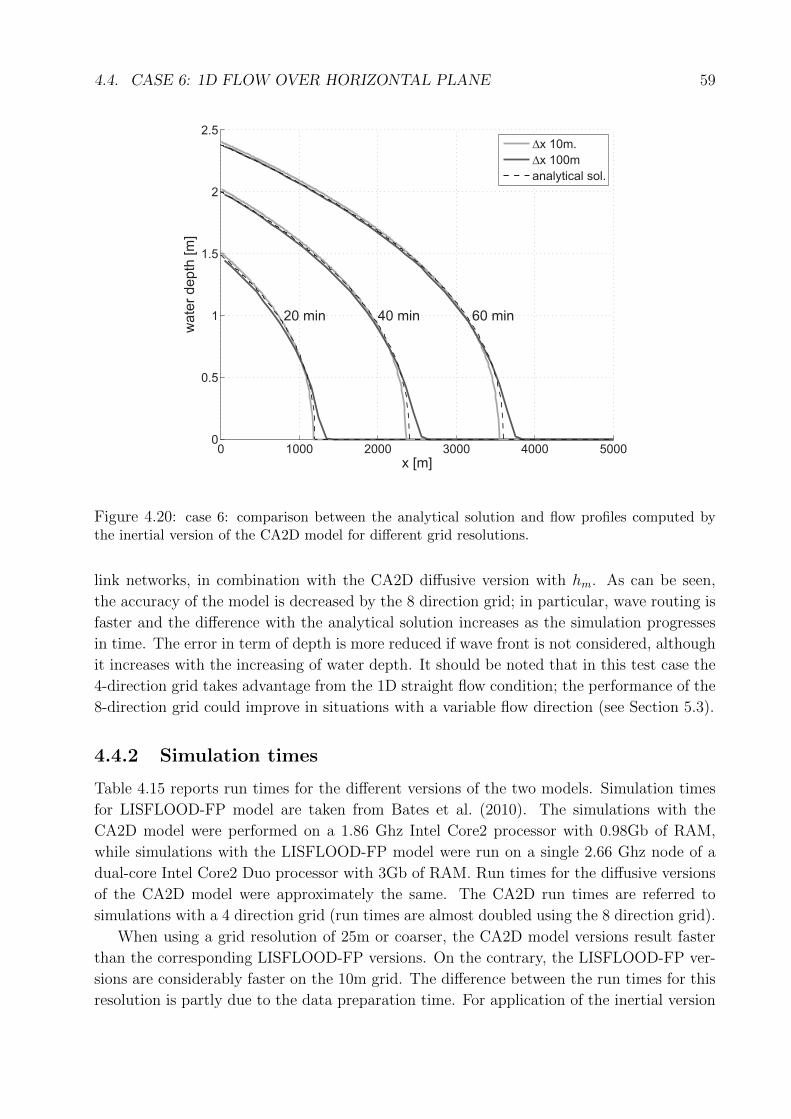
4.4. CASE 6: 1D FLOW OVER HORIZONTAL PLANE 59
0 1000 2000 3000 4000 50000
0.5
1
1.5
2
2.5
20 min 40 min 60 min
wate
rdepth
[m]
x [m]
∆x 10m.
∆x 100m
analytical sol.
Figure 4.20: case 6: comparison between the analytical solution and flow profiles computed bythe inertial version of the CA2D model for different grid resolutions.
link networks, in combination with the CA2D diffusive version with hm. As can be seen,
the accuracy of the model is decreased by the 8 direction grid; in particular, wave routing is
faster and the difference with the analytical solution increases as the simulation progresses
in time. The error in term of depth is more reduced if wave front is not considered, although
it increases with the increasing of water depth. It should be noted that in this test case the
4-direction grid takes advantage from the 1D straight flow condition; the performance of the
8-direction grid could improve in situations with a variable flow direction (see Section 5.3).
4.4.2 Simulation times
Table 4.15 reports run times for the different versions of the two models. Simulation times
for LISFLOOD-FP model are taken from Bates et al. (2010). The simulations with the
CA2D model were performed on a 1.86 Ghz Intel Core2 processor with 0.98Gb of RAM,
while simulations with the LISFLOOD-FP model were run on a single 2.66 Ghz node of a
dual-core Intel Core2 Duo processor with 3Gb of RAM. Run times for the diffusive versions
of the CA2D model were approximately the same. The CA2D run times are referred to
simulations with a 4 direction grid (run times are almost doubled using the 8 direction grid).
When using a grid resolution of 25m or coarser, the CA2D model versions result faster
than the corresponding LISFLOOD-FP versions. On the contrary, the LISFLOOD-FP ver-
sions are considerably faster on the 10m grid. The difference between the run times for this
resolution is partly due to the data preparation time. For application of the inertial version
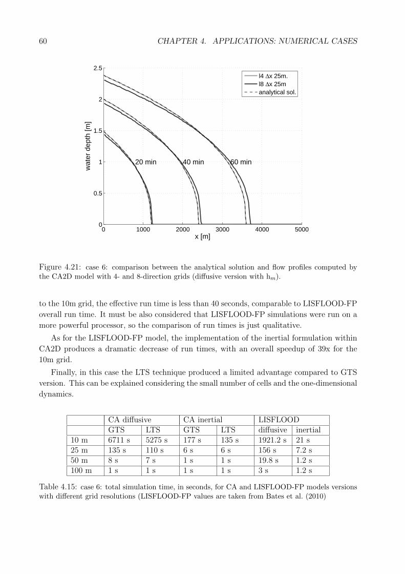
60 CHAPTER 4. APPLICATIONS: NUMERICAL CASES
0 1000 2000 3000 4000 50000
0.5
1
1.5
2
2.5
20 min 40 min 60 min
wat
er d
epth
[m]
x [m]
l4 ∆x 25m.l8 ∆x 25manalytical sol.
Figure 4.21: case 6: comparison between the analytical solution and flow profiles computed bythe CA2D model with 4- and 8-direction grids (diffusive version with hm).
to the 10m grid, the effective run time is less than 40 seconds, comparable to LISFLOOD-FP
overall run time. It must be also considered that LISFLOOD-FP simulations were run on a
more powerful processor, so the comparison of run times is just qualitative.
As for the LISFLOOD-FP model, the implementation of the inertial formulation within
CA2D produces a dramatic decrease of run times, with an overall speedup of 39x for the
10m grid.
Finally, in this case the LTS technique produced a limited advantage compared to GTS
version. This can be explained considering the small number of cells and the one-dimensional
dynamics.
CA diffusive CA inertial LISFLOODGTS LTS GTS LTS diffusive inertial
10 m 6711 s 5275 s 177 s 135 s 1921.2 s 21 s25 m 135 s 110 s 6 s 6 s 156 s 7.2 s50 m 8 s 7 s 1 s 1 s 19.8 s 1.2 s100 m 1 s 1 s 1 s 1 s 3 s 1.2 s
Table 4.15: case 6: total simulation time, in seconds, for CA and LISFLOOD-FP models versionswith different grid resolutions (LISFLOOD-FP values are taken from Bates et al. (2010)
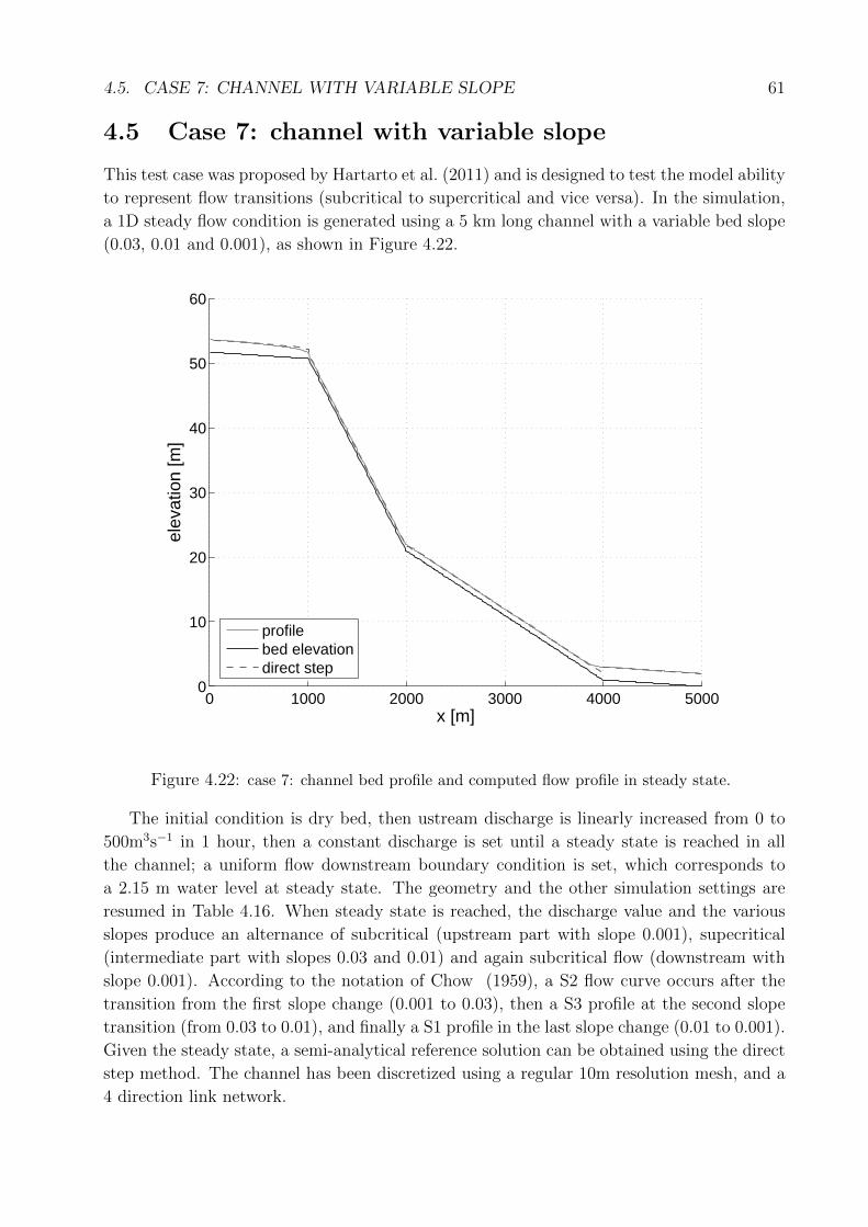
4.5. CASE 7: CHANNEL WITH VARIABLE SLOPE 61
4.5 Case 7: channel with variable slope
This test case was proposed by Hartarto et al. (2011) and is designed to test the model ability
to represent flow transitions (subcritical to supercritical and vice versa). In the simulation,
a 1D steady flow condition is generated using a 5 km long channel with a variable bed slope
(0.03, 0.01 and 0.001), as shown in Figure 4.22.
0 1000 2000 3000 4000 50000
10
20
30
40
50
60
elev
atio
n [m
]
x [m]
profilebed elevationdirect step
Figure 4.22: case 7: channel bed profile and computed flow profile in steady state.
The initial condition is dry bed, then ustream discharge is linearly increased from 0 to
500m3s−1 in 1 hour, then a constant discharge is set until a steady state is reached in all
the channel; a uniform flow downstream boundary condition is set, which corresponds to
a 2.15 m water level at steady state. The geometry and the other simulation settings are
resumed in Table 4.16. When steady state is reached, the discharge value and the various
slopes produce an alternance of subcritical (upstream part with slope 0.001), supecritical
(intermediate part with slopes 0.03 and 0.01) and again subcritical flow (downstream with
slope 0.001). According to the notation of Chow (1959), a S2 flow curve occurs after the
transition from the first slope change (0.001 to 0.03), then a S3 profile at the second slope
transition (from 0.03 to 0.01), and finally a S1 profile in the last slope change (0.01 to 0.001).
Given the steady state, a semi-analytical reference solution can be obtained using the direct
step method. The channel has been discretized using a regular 10m resolution mesh, and a
4 direction link network.
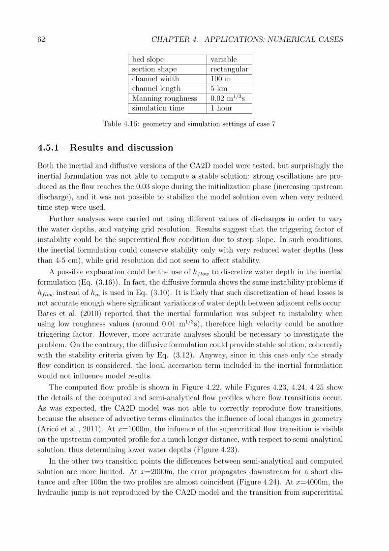
62 CHAPTER 4. APPLICATIONS: NUMERICAL CASES
bed slope variablesection shape rectangularchannel width 100 mchannel length 5 km
Manning roughness 0.02 m1/3ssimulation time 1 hour
Table 4.16: geometry and simulation settings of case 7
4.5.1 Results and discussion
Both the inertial and diffusive versions of the CA2D model were tested, but surprisingly the
inertial formulation was not able to compute a stable solution: strong oscillations are pro-
duced as the flow reaches the 0.03 slope during the initialization phase (increasing upstream
discharge), and it was not possible to stabilize the model solution even when very reduced
time step were used.
Further analyses were carried out using different values of discharges in order to vary
the water depths, and varying grid resolution. Results suggest that the triggering factor of
instability could be the supercritical flow condition due to steep slope. In such conditions,
the inertial formulation could conserve stability only with very reduced water depths (less
than 4-5 cm), while grid resolution did not seem to affect stability.
A possible explanation could be the use of hflow to discretize water depth in the inertial
formulation (Eq. (3.16)). In fact, the diffusive formula shows the same instability problems if
hflow instead of hm is used in Eq. (3.10). It is likely that such discretization of head losses is
not accurate enough where significant variations of water depth between adjacent cells occur.
Bates et al. (2010) reported that the inertial formulation was subject to instability when
using low roughness values (around 0.01 m1/3s), therefore high velocity could be another
triggering factor. However, more accurate analyses should be necessary to investigate the
problem. On the contrary, the diffusive formulation could provide stable solution, coherently
with the stability criteria given by Eq. (3.12). Anyway, since in this case only the steady
flow condition is considered, the local acceration term included in the inertial formulation
would not influence model results.
The computed flow profile is shown in Figure 4.22, while Figures 4.23, 4.24, 4.25 show
the details of the computed and semi-analytical flow profiles where flow transitions occur.
As was expected, the CA2D model was not able to correctly reproduce flow transitions,
because the absence of advective terms eliminates the influence of local changes in geometry
(Arico et al., 2011). At x=1000m, the infuence of the supercritical flow transition is visible
on the upstream computed profile for a much longer distance, with respect to semi-analytical
solution, thus determining lower water depths (Figure 4.23).
In the other two transition points the differences between semi-analytical and computed
solution are more limited. At x=2000m, the error propagates downstream for a short dis-
tance and after 100m the two profiles are almost coincident (Figure 4.24). At x=4000m, the
hydraulic jump is not reproduced by the CA2D model and the transition from supercritital
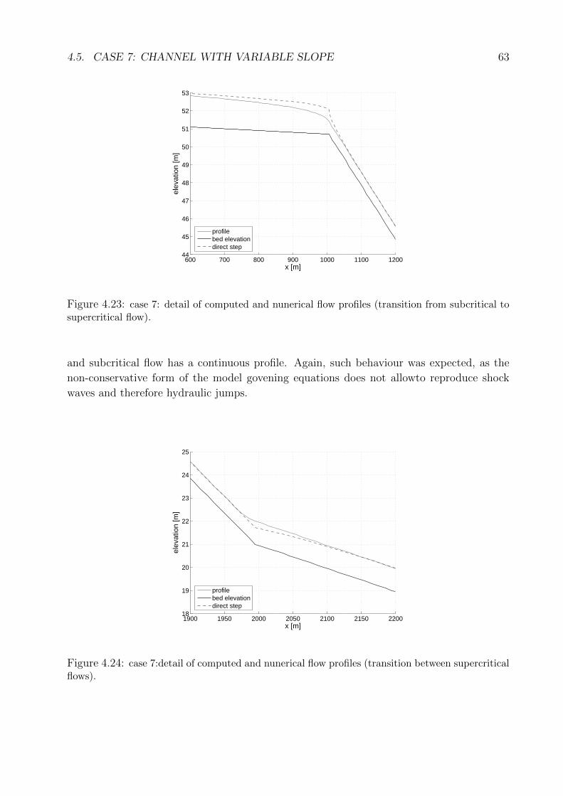
4.5. CASE 7: CHANNEL WITH VARIABLE SLOPE 63
600 700 800 900 1000 1100 120044
45
46
47
48
49
50
51
52
53
elev
atio
n [m
]
x [m]
profilebed elevationdirect step
Figure 4.23: case 7: detail of computed and nunerical flow profiles (transition from subcritical tosupercritical flow).
and subcritical flow has a continuous profile. Again, such behaviour was expected, as the
non-conservative form of the model govening equations does not allowto reproduce shock
waves and therefore hydraulic jumps.
1900 1950 2000 2050 2100 2150 220018
19
20
21
22
23
24
25
elev
atio
n [m
]
x [m]
profilebed elevationdirect step
Figure 4.24: case 7:detail of computed and nunerical flow profiles (transition between supercriticalflows).

64 CHAPTER 4. APPLICATIONS: NUMERICAL CASES
3800 3850 3900 3950 4000 4050 4100 4150 42000.5
1
1.5
2
2.5
3
3.5
4
elev
atio
n [m
]
x [m]
profilebed elevationdirect step
Figure 4.25: case 7:detail of computed and nunerical flow profiles (hydraulic jump).
4.6 Overall considerations about the models
The analysis of the numerical cases allowed to investigate the reliability of the CA2D and
IFD-GGA models, and their performance in different flow conditions. Overall results high-
lighted relevant differences between the performance of the two models, that are below
summarized.
4.6.1 performance of the CA2D model
The overall performance of the CA2D model was very satisfactory. First of all, the model
proved to be robust and could be applied in all the considered test cases. Run times were
small and comparable to other established hydraulic models. As expected, the accuracy
of CA2D varied according to flow conditons. The model provided accurate results in one-
dimensional flow conditions over with mild slopes, as well as in reproducing overland flow
conditions, with reduced water depths and steep slopes. The model performance was less
satisfactory when flow transitions over steep slopes were simulated, and relevant local errors
were observed, due to the non-conservative governing equations. When applied to two-
dimensional numerical cases, the model showed some limitations with respect to the fully
dyinamic CCHE2D model. Such results were partly expected since the original formulation
of the model does not account for acceleration and advection effects. However, in 2D cases
the magnitude of observed errors was limited and below the typical uncertainty level of data
and observations in actual flood events, e.g. topography and inundation extent maps.
In order to increase model performance and to reduce run times, two existing techniques
were implemented and tested, both with overall good results. The incorporation of a local
adaptive time step algorithm reduced the computation time in all the simulations, with
no loss of accuracy in the results. On the other hand, the implementation of the inertial

4.6. OVERALL CONSIDERATIONS ABOUT THE MODELS 65
formulation proposed by Bates et al. (2010) was even more effective, reducing computation
times up to 97%. However, compared to the original diffusive formulation, the inertial
formulation did not improve the accuracy of results, and the formulation showed serious
instability problems when applied over steep slopes. The analysis of two dimensional cases
suggested that the inclusion of the advection terms within the model equations will be
necessary for a more accurate simulation of flow dynamics. Given these good results, the
CA2D model has been further applied to reproduce flood events and scenarios (Chapter 5).
4.6.2 performance of the IFD-GGA model
The overall results of the IFD-GGA model in the considered numerical cases were not satis-
factory. The model performed well in simple 1D cases with a limited number of cells, both
in terms of accuracy and reliability of solution methods. On the contrary, in the 2D cases
the versions of the model using Jacobi solution scheme had serious convergence problems
that prevented its application. Better results were obtained by applying the CGM, however
the resulting computation times were too slow with respect both to the CA2D model and
the fully dynamic CCHE2D model. Hence, it was decided to interrupt the work on the
IFD-GGA model, and reconsider its development (see Chapter 6).

66 CHAPTER 4. APPLICATIONS: NUMERICAL CASES
Chapter 5
APPLICATIONS: FLOOD EVENTS
AND SCENARIOS
Different issues are currently being addressed in research applications of hydraulic models
in flood events and flood scenarios. Among them, the assessment of model performances
is a key issue to improve the reliability of flood inundation studies. In fact, the current
large amount of topographic information (Section 2.8) is not supported by a comparable
availability of field information regarding the development and the dynamics of flood events.
Experimental data of flood extent, water levels and velocities are generally limited in terms of
spatial and temporal coverage, and affected by a significant uncertainty (Hunter et al., 2007).
In some cases, different types of observed data were available to perform model validation
and calibration (Hunter et al., 2005a; Werner et al., 2005; Bates et al., 2006; Neal et al.,
2009a). However, even in these data-rich events the sparsity and uncertainty of observed
data did not allow for rigorous assessment of model results. As a result, possible limitations
of a simplifed model can be disguised by the calibration procedure, while a more complex
model can not exploit its better potential because of data scarcity (Bates et al., 2004; Horritt
et al., 2007; Di Baldassarre et al., 2009b). This was confimed in different research works
where the performances of 1D or diffusive 2D models were comparable to fully dynamic 2D
models, as mentioned in Section 2.8.
In this framework, the evaluation procedure of a 2D model should include applications
to different flood events and scenarios, with the purpose of testing model performance using
typical data set for model construction and validation. This is carried out in the present
chapter by analyzing four test cases which differs in terms of location, topography config-
uration, extent and ongoing flow processes. Only applications of the CA2D model are here
described, given the relevant problems of the IFD-GGA model highlighted in Chapter 4.
Although during the research period CA2D has been applied in several flood risk and flood
hazard analyses, for reasons of conciseness only a limited number of applications are here
reported. These applications have been selected because they provide a good overview of
model capabilities; moreover, observed data are available for model evaluation.
Section 5.1 describes CA2D application in a lowland rural flood event originated by a
levee breach, where overland 2D flow is dominant. In section 5.2 the model is used to
67
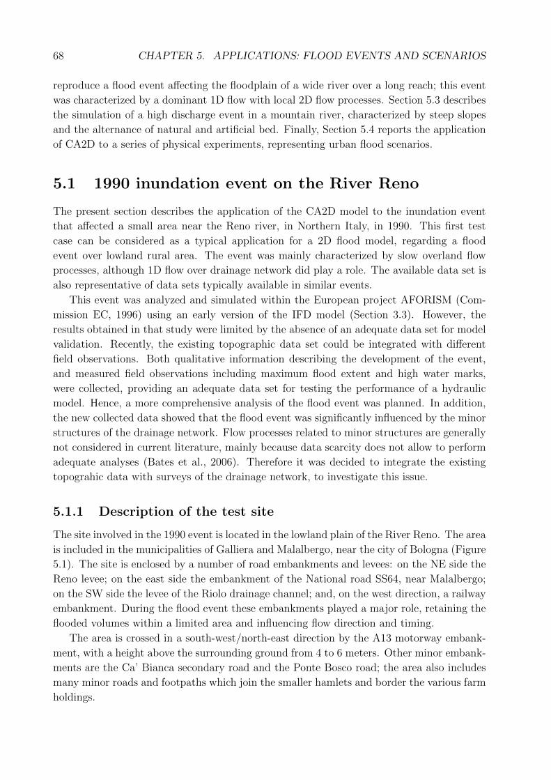
68 CHAPTER 5. APPLICATIONS: FLOOD EVENTS AND SCENARIOS
reproduce a flood event affecting the floodplain of a wide river over a long reach; this event
was characterized by a dominant 1D flow with local 2D flow processes. Section 5.3 describes
the simulation of a high discharge event in a mountain river, characterized by steep slopes
and the alternance of natural and artificial bed. Finally, Section 5.4 reports the application
of CA2D to a series of physical experiments, representing urban flood scenarios.
5.1 1990 inundation event on the River Reno
The present section describes the application of the CA2D model to the inundation event
that affected a small area near the Reno river, in Northern Italy, in 1990. This first test
case can be considered as a typical application for a 2D flood model, regarding a flood
event over lowland rural area. The event was mainly characterized by slow overland flow
processes, although 1D flow over drainage network did play a role. The available data set is
also representative of data sets typically available in similar events.
This event was analyzed and simulated within the European project AFORISM (Com-
mission EC, 1996) using an early version of the IFD model (Section 3.3). However, the
results obtained in that study were limited by the absence of an adequate data set for model
validation. Recently, the existing topographic data set could be integrated with different
field observations. Both qualitative information describing the development of the event,
and measured field observations including maximum flood extent and high water marks,
were collected, providing an adequate data set for testing the performance of a hydraulic
model. Hence, a more comprehensive analysis of the flood event was planned. In addition,
the new collected data showed that the flood event was significantly influenced by the minor
structures of the drainage network. Flow processes related to minor structures are generally
not considered in current literature, mainly because data scarcity does not allow to perform
adequate analyses (Bates et al., 2006). Therefore it was decided to integrate the existing
topograhic data with surveys of the drainage network, to investigate this issue.
5.1.1 Description of the test site
The site involved in the 1990 event is located in the lowland plain of the River Reno. The area
is included in the municipalities of Galliera and Malalbergo, near the city of Bologna (Figure
5.1). The site is enclosed by a number of road embankments and levees: on the NE side the
Reno levee; on the east side the embankment of the National road SS64, near Malalbergo;
on the SW side the levee of the Riolo drainage channel; and, on the west direction, a railway
embankment. During the flood event these embankments played a major role, retaining the
flooded volumes within a limited area and influencing flow direction and timing.
The area is crossed in a south-west/north-east direction by the A13 motorway embank-
ment, with a height above the surrounding ground from 4 to 6 meters. Other minor embank-
ments are the Ca’ Bianca secondary road and the Ponte Bosco road; the area also includes
many minor roads and footpaths which join the smaller hamlets and border the various farm
holdings.
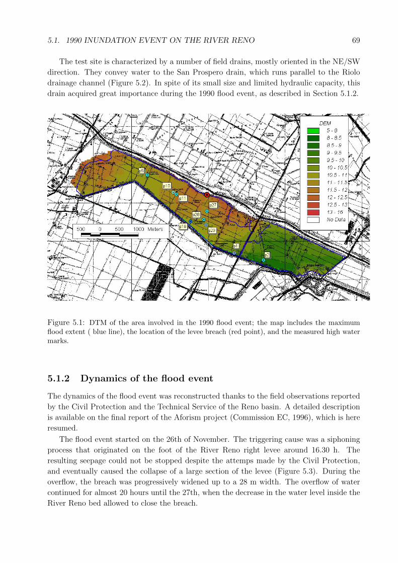
5.1. 1990 INUNDATION EVENT ON THE RIVER RENO 69
The test site is characterized by a number of field drains, mostly oriented in the NE/SW
direction. They convey water to the San Prospero drain, which runs parallel to the Riolo
drainage channel (Figure 5.2). In spite of its small size and limited hydraulic capacity, this
drain acquired great importance during the 1990 flood event, as described in Section 5.1.2.
Figure 5.1: DTM of the area involved in the 1990 flood event; the map includes the maximumflood extent ( blue line), the location of the levee breach (red point), and the measured high watermarks.
5.1.2 Dynamics of the flood event
The dynamics of the flood event was reconstructed thanks to the field observations reported
by the Civil Protection and the Technical Service of the Reno basin. A detailed description
is available on the final report of the Aforism project (Commission EC, 1996), which is here
resumed.
The flood event started on the 26th of November. The triggering cause was a siphoning
process that originated on the foot of the River Reno right levee around 16.30 h. The
resulting seepage could not be stopped despite the attemps made by the Civil Protection,
and eventually caused the collapse of a large section of the levee (Figure 5.3). During the
overflow, the breach was progressively widened up to a 28 m width. The overflow of water
continued for almost 20 hours until the 27th, when the decrease in the water level inside the
River Reno bed allowed to close the breach.
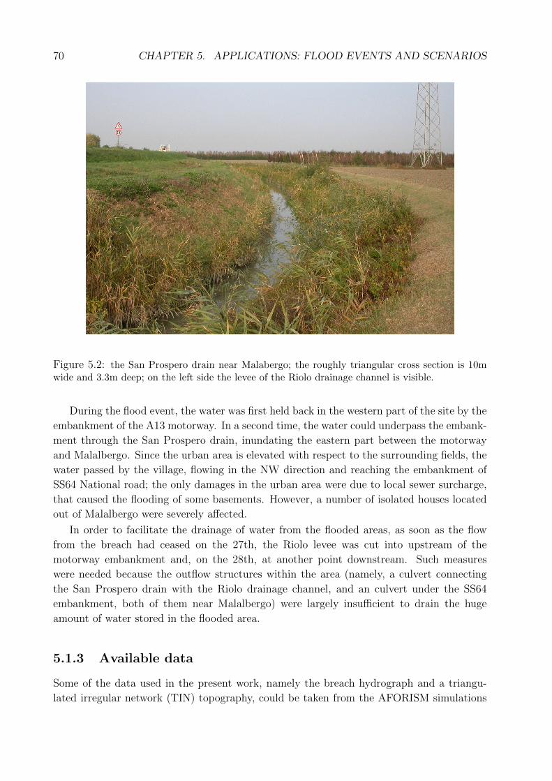
70 CHAPTER 5. APPLICATIONS: FLOOD EVENTS AND SCENARIOS
Figure 5.2: the San Prospero drain near Malabergo; the roughly triangular cross section is 10mwide and 3.3m deep; on the left side the levee of the Riolo drainage channel is visible.
During the flood event, the water was first held back in the western part of the site by the
embankment of the A13 motorway. In a second time, the water could underpass the embank-
ment through the San Prospero drain, inundating the eastern part between the motorway
and Malalbergo. Since the urban area is elevated with respect to the surrounding fields, the
water passed by the village, flowing in the NW direction and reaching the embankment of
SS64 National road; the only damages in the urban area were due to local sewer surcharge,
that caused the flooding of some basements. However, a number of isolated houses located
out of Malalbergo were severely affected.
In order to facilitate the drainage of water from the flooded areas, as soon as the flow
from the breach had ceased on the 27th, the Riolo levee was cut into upstream of the
motorway embankment and, on the 28th, at another point downstream. Such measures
were needed because the outflow structures within the area (namely, a culvert connecting
the San Prospero drain with the Riolo drainage channel, and an culvert under the SS64
embankment, both of them near Malalbergo) were largely insufficient to drain the huge
amount of water stored in the flooded area.
5.1.3 Available data
Some of the data used in the present work, namely the breach hydrograph and a triangu-
lated irregular network (TIN) topography, could be taken from the AFORISM simulations
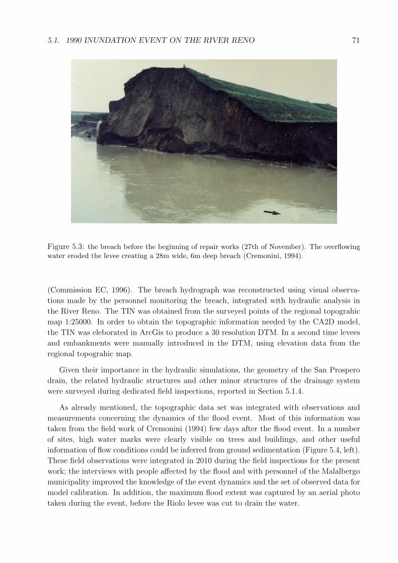
5.1. 1990 INUNDATION EVENT ON THE RIVER RENO 71
Figure 5.3: the breach before the beginning of repair works (27th of November). The overflowingwater eroded the levee creating a 28m wide, 6m deep breach (Cremonini, 1994).
(Commission EC, 1996). The breach hydrograph was reconstructed using visual observa-
tions made by the personnel monitoring the breach, integrated with hydraulic analysis in
the River Reno. The TIN was obtained from the surveyed points of the regional topograhic
map 1:25000. In order to obtain the topographic information needed by the CA2D model,
the TIN was eleborated in ArcGis to produce a 30 resolution DTM. In a second time levees
and embankments were manually introduced in the DTM, using elevation data from the
regional topograhic map.
Given their importance in the hydraulic simulations, the geometry of the San Prospero
drain, the related hydraulic structures and other minor structures of the drainage system
were surveyed during dedicated field inspections, reported in Section 5.1.4.
As already mentioned, the topographic data set was integrated with observations and
measurements concerning the dynamics of the flood event. Most of this information was
taken from the field work of Cremonini (1994) few days after the flood event. In a number
of sites, high water marks were clearly visible on trees and buildings, and other useful
information of flow conditions could be inferred from ground sedimentation (Figure 5.4, left).
These field observations were integrated in 2010 during the field inspections for the present
work; the interviews with people affected by the flood and with personnel of the Malalbergo
municipality improved the knowledge of the event dynamics and the set of observed data for
model calibration. In addition, the maximum flood extent was captured by an aerial photo
taken during the event, before the Riolo levee was cut to drain the water.
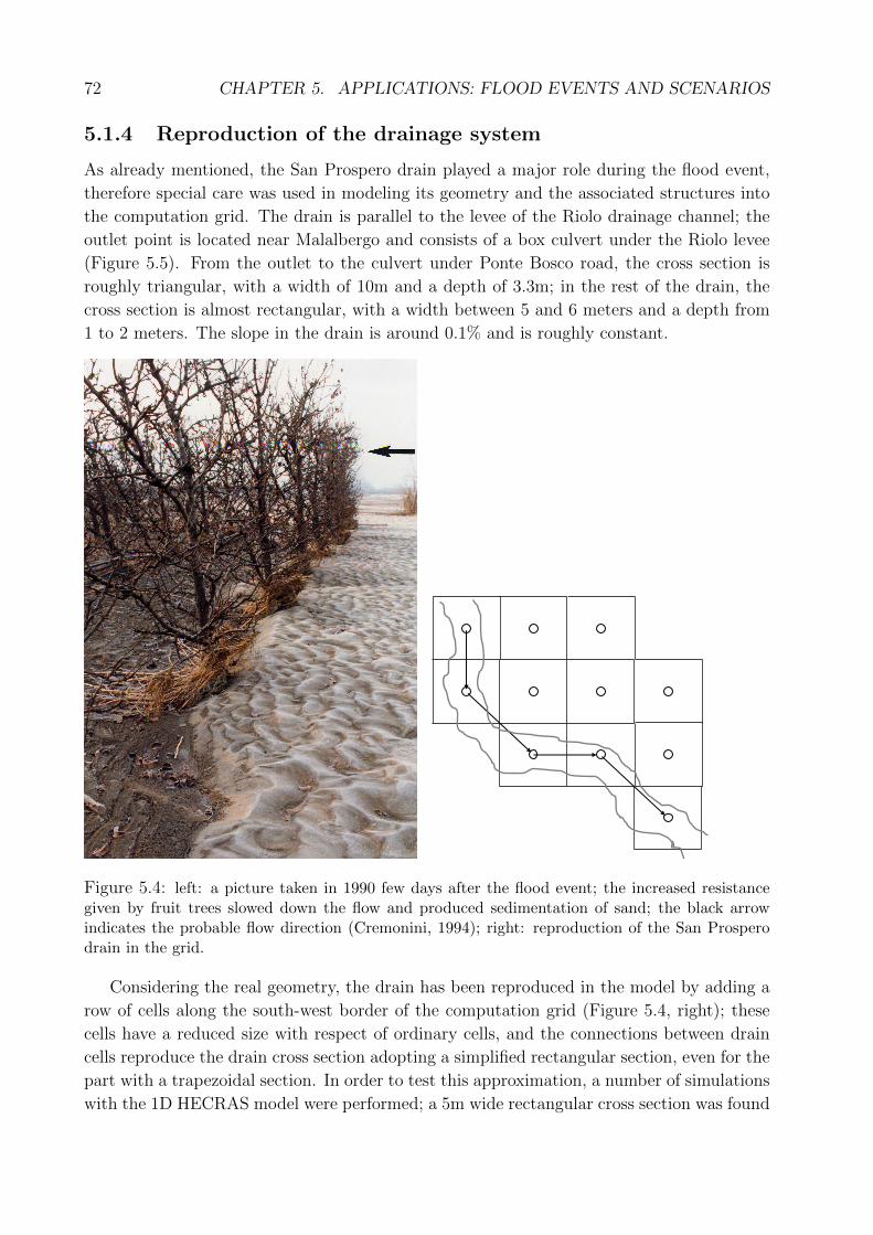
72 CHAPTER 5. APPLICATIONS: FLOOD EVENTS AND SCENARIOS
5.1.4 Reproduction of the drainage system
As already mentioned, the San Prospero drain played a major role during the flood event,
therefore special care was used in modeling its geometry and the associated structures into
the computation grid. The drain is parallel to the levee of the Riolo drainage channel; the
outlet point is located near Malalbergo and consists of a box culvert under the Riolo levee
(Figure 5.5). From the outlet to the culvert under Ponte Bosco road, the cross section is
roughly triangular, with a width of 10m and a depth of 3.3m; in the rest of the drain, the
cross section is almost rectangular, with a width between 5 and 6 meters and a depth from
1 to 2 meters. The slope in the drain is around 0.1% and is roughly constant.
schema di calcolo Reno 1990schema di calcolo Reno 1990
Figure 5.4: left: a picture taken in 1990 few days after the flood event; the increased resistancegiven by fruit trees slowed down the flow and produced sedimentation of sand; the black arrowindicates the probable flow direction (Cremonini, 1994); right: reproduction of the San Prosperodrain in the grid.
Considering the real geometry, the drain has been reproduced in the model by adding a
row of cells along the south-west border of the computation grid (Figure 5.4, right); these
cells have a reduced size with respect of ordinary cells, and the connections between drain
cells reproduce the drain cross section adopting a simplified rectangular section, even for the
part with a trapezoidal section. In order to test this approximation, a number of simulations
with the 1D HECRAS model were performed; a 5m wide rectangular cross section was found
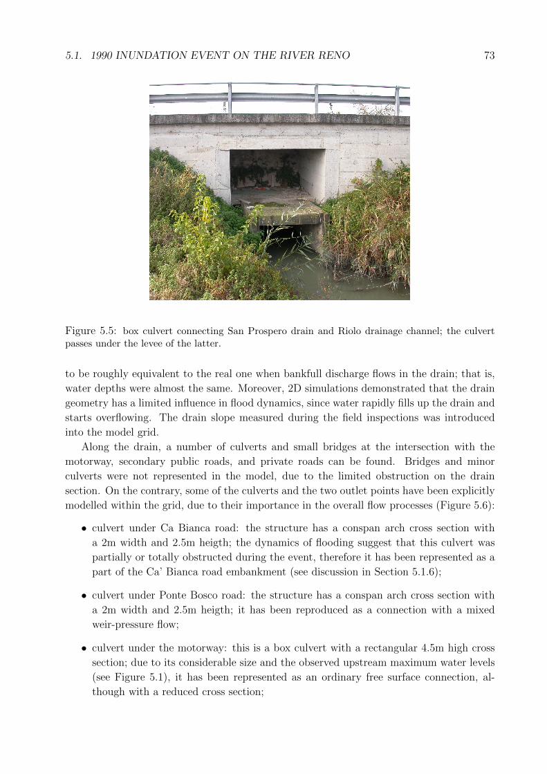
5.1. 1990 INUNDATION EVENT ON THE RIVER RENO 73
Figure 5.5: box culvert connecting San Prospero drain and Riolo drainage channel; the culvertpasses under the levee of the latter.
to be roughly equivalent to the real one when bankfull discharge flows in the drain; that is,
water depths were almost the same. Moreover, 2D simulations demonstrated that the drain
geometry has a limited influence in flood dynamics, since water rapidly fills up the drain and
starts overflowing. The drain slope measured during the field inspections was introduced
into the model grid.
Along the drain, a number of culverts and small bridges at the intersection with the
motorway, secondary public roads, and private roads can be found. Bridges and minor
culverts were not represented in the model, due to the limited obstruction on the drain
section. On the contrary, some of the culverts and the two outlet points have been explicitly
modelled within the grid, due to their importance in the overall flow processes (Figure 5.6):
• culvert under Ca Bianca road: the structure has a conspan arch cross section with
a 2m width and 2.5m heigth; the dynamics of flooding suggest that this culvert was
partially or totally obstructed during the event, therefore it has been represented as a
part of the Ca’ Bianca road embankment (see discussion in Section 5.1.6);
• culvert under Ponte Bosco road: the structure has a conspan arch cross section with
a 2m width and 2.5m heigth; it has been reproduced as a connection with a mixed
weir-pressure flow;
• culvert under the motorway: this is a box culvert with a rectangular 4.5m high cross
section; due to its considerable size and the observed upstream maximum water levels
(see Figure 5.1), it has been represented as an ordinary free surface connection, al-
though with a reduced cross section;
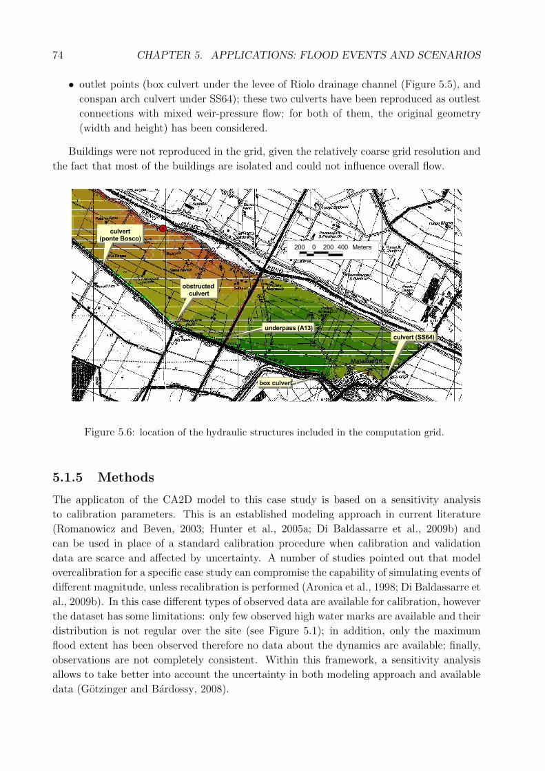
74 CHAPTER 5. APPLICATIONS: FLOOD EVENTS AND SCENARIOS
• outlet points (box culvert under the levee of Riolo drainage channel (Figure 5.5), and
conspan arch culvert under SS64); these two culverts have been reproduced as outlest
connections with mixed weir-pressure flow; for both of them, the original geometry
(width and height) has been considered.
Buildings were not reproduced in the grid, given the relatively coarse grid resolution and
the fact that most of the buildings are isolated and could not influence overall flow.
Figure 5.6: location of the hydraulic structures included in the computation grid.
5.1.5 Methods
The applicaton of the CA2D model to this case study is based on a sensitivity analysis
to calibration parameters. This is an established modeling approach in current literature
(Romanowicz and Beven, 2003; Hunter et al., 2005a; Di Baldassarre et al., 2009b) and
can be used in place of a standard calibration procedure when calibration and validation
data are scarce and affected by uncertainty. A number of studies pointed out that model
overcalibration for a specific case study can compromise the capability of simulating events of
different magnitude, unless recalibration is performed (Aronica et al., 1998; Di Baldassarre et
al., 2009b). In this case different types of observed data are available for calibration, however
the dataset has some limitations: only few observed high water marks are available and their
distribution is not regular over the site (see Figure 5.1); in addition, only the maximum
flood extent has been observed therefore no data about the dynamics are available; finally,
observations are not completely consistent. Within this framework, a sensitivity analysis
allows to take better into account the uncertainty in both modeling approach and available
data (Gotzinger and Bardossy, 2008).
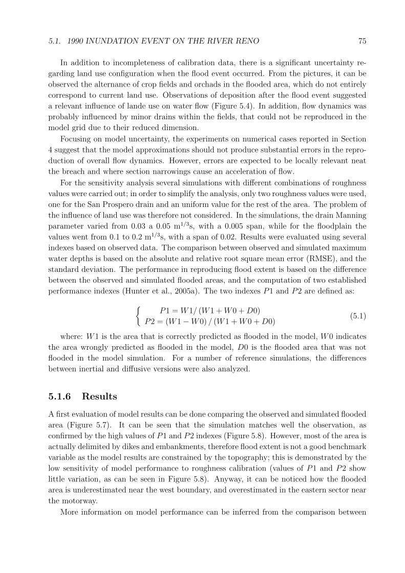
5.1. 1990 INUNDATION EVENT ON THE RIVER RENO 75
In addition to incompleteness of calibration data, there is a significant uncertainty re-
garding land use configuration when the flood event occurred. From the pictures, it can be
observed the alternance of crop fields and orchads in the flooded area, which do not entirely
correspond to current land use. Observations of deposition after the flood event suggested
a relevant influence of lande use on water flow (Figure 5.4). In addition, flow dynamics was
probably influenced by minor drains within the fields, that could not be reproduced in the
model grid due to their reduced dimension.
Focusing on model uncertainty, the experiments on numerical cases reported in Section
4 suggest that the model approximations should not produce substantial errors in the repro-
duction of overall flow dynamics. However, errors are expected to be locally relevant neat
the breach and where section narrowings cause an acceleration of flow.
For the sensitivity analysis several simulations with different combinations of roughness
values were carried out; in order to simplify the analysis, only two roughness values were used,
one for the San Prospero drain and an uniform value for the rest of the area. The problem of
the influence of land use was therefore not considered. In the simulations, the drain Manning
parameter varied from 0.03 a 0.05 m1/3s, with a 0.005 span, while for the floodplain the
values went from 0.1 to 0.2 m1/3s, with a span of 0.02. Results were evaluated using several
indexes based on observed data. The comparison between observed and simulated maximum
water depths is based on the absolute and relative root square mean error (RMSE), and the
standard deviation. The performance in reproducing flood extent is based on the difference
between the observed and simulated flooded areas, and the computation of two established
performance indexes (Hunter et al., 2005a). The two indexes P1 and P2 are defined as:P1 = W1/ (W1 +W0 +D0)
P2 = (W1−W0) / (W1 +W0 +D0)(5.1)
where: W1 is the area that is correctly predicted as flooded in the model, W0 indicates
the area wrongly predicted as flooded in the model, D0 is the flooded area that was not
flooded in the model simulation. For a number of reference simulations, the differences
between inertial and diffusive versions were also analyzed.
5.1.6 Results
A first evaluation of model results can be done comparing the observed and simulated flooded
area (Figure 5.7). It can be seen that the simulation matches well the observation, as
confirmed by the high values of P1 and P2 indexes (Figure 5.8). However, most of the area is
actually delimited by dikes and embankments, therefore flood extent is not a good benchmark
variable as the model results are constrained by the topography; this is demonstrated by the
low sensitivity of model performance to roughness calibration (values of P1 and P2 show
little variation, as can be seen in Figure 5.8). Anyway, it can be noticed how the flooded
area is underestimated near the west boundary, and overestimated in the eastern sector near
the motorway.
More information on model performance can be inferred from the comparison between
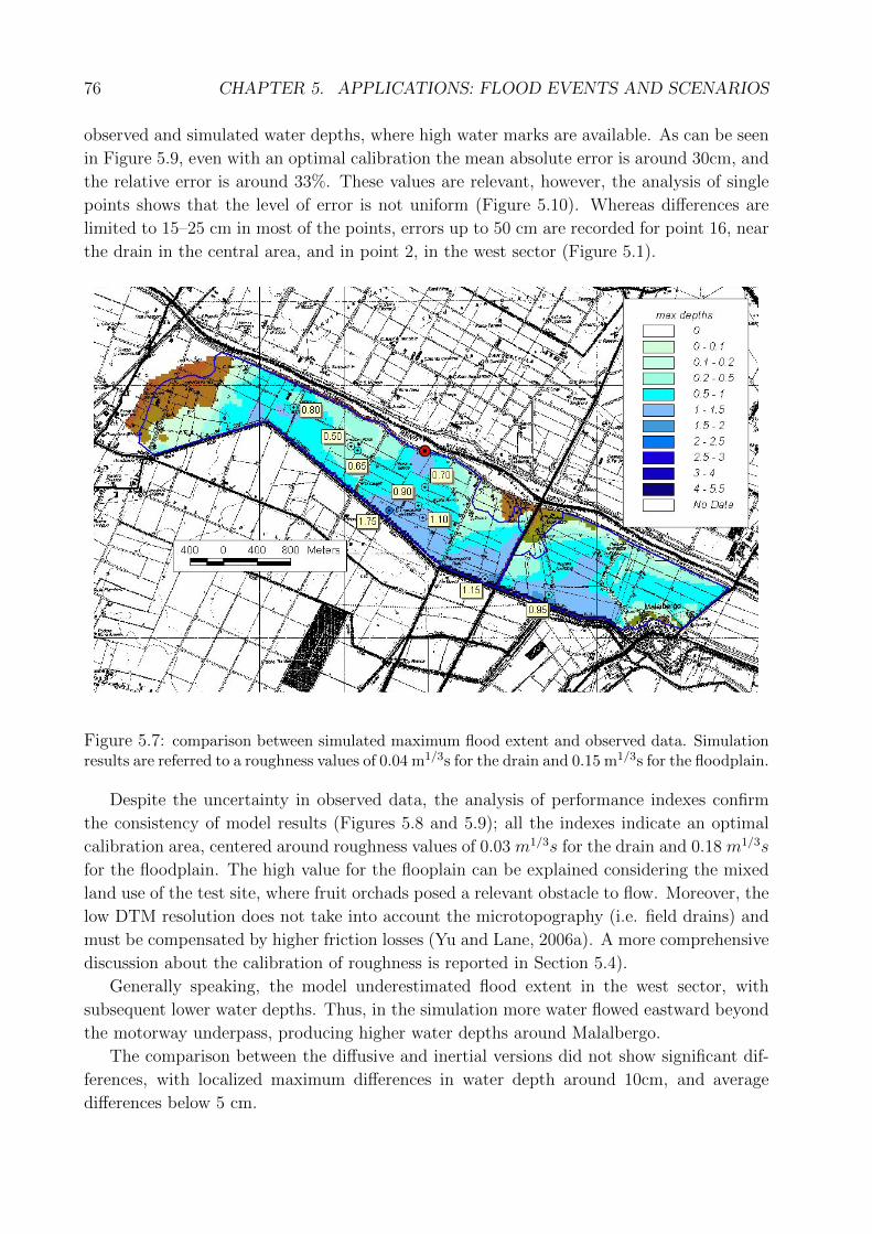
76 CHAPTER 5. APPLICATIONS: FLOOD EVENTS AND SCENARIOS
observed and simulated water depths, where high water marks are available. As can be seen
in Figure 5.9, even with an optimal calibration the mean absolute error is around 30cm, and
the relative error is around 33%. These values are relevant, however, the analysis of single
points shows that the level of error is not uniform (Figure 5.10). Whereas differences are
limited to 15–25 cm in most of the points, errors up to 50 cm are recorded for point 16, near
the drain in the central area, and in point 2, in the west sector (Figure 5.1).
Figure 5.7: comparison between simulated maximum flood extent and observed data. Simulationresults are referred to a roughness values of 0.04 m1/3s for the drain and 0.15 m1/3s for the floodplain.
Despite the uncertainty in observed data, the analysis of performance indexes confirm
the consistency of model results (Figures 5.8 and 5.9); all the indexes indicate an optimal
calibration area, centered around roughness values of 0.03 m1/3s for the drain and 0.18 m1/3s
for the floodplain. The high value for the flooplain can be explained considering the mixed
land use of the test site, where fruit orchads posed a relevant obstacle to flow. Moreover, the
low DTM resolution does not take into account the microtopography (i.e. field drains) and
must be compensated by higher friction losses (Yu and Lane, 2006a). A more comprehensive
discussion about the calibration of roughness is reported in Section 5.4).
Generally speaking, the model underestimated flood extent in the west sector, with
subsequent lower water depths. Thus, in the simulation more water flowed eastward beyond
the motorway underpass, producing higher water depths around Malalbergo.
The comparison between the diffusive and inertial versions did not show significant dif-
ferences, with localized maximum differences in water depth around 10cm, and average
differences below 5 cm.
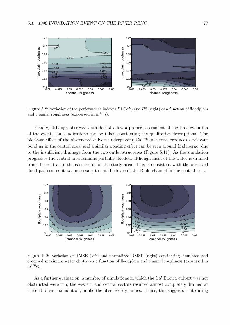
5.1. 1990 INUNDATION EVENT ON THE RIVER RENO 77
0.885
0.8860.886
0.8870.8870.8880.8880.8890.889
0.890.89
0.8910.891
0.892
0.892
0.893
channel roughness
flood
plai
n ro
ughn
ess
0.02 0.025 0.03 0.035 0.04 0.045 0.050.1
0.12
0.14
0.16
0.18
0.2
0.220.844
0.844
0.846
0.846
0.846
0.8460.8480.850.852
channel roughness
flood
plai
n ro
ughn
ess
0.02 0.025 0.03 0.035 0.04 0.045 0.050.1
0.12
0.14
0.16
0.18
0.2
0.22
Figure 5.8: variation of the performance indexes P1 (left) and P2 (right) as a function of floodplainand channel roughness (expressed in m1/3s).
Finally, although observed data do not allow a proper assessment of the time evolution
of the event, some indications can be taken considering the qualitative descriptions. The
blockage effect of the obstructed culvert underpassing Ca’ Bianca road produces a relevant
ponding in the central area, and a similar ponding effect can be seen around Malabergo, due
to the insufficient drainage from the two outlet structures (Figure 5.11). As the simulation
progresses the central area remains partially flooded, although most of the water is drained
from the central to the east sector of the study area. This is consistent with the observed
flood pattern, as it was necessary to cut the levee of the Riolo channel in the central area.
0.3
0.3
0.31
0.31
0.31
0.32
0.320.33
0.33
0.34
channel roughness
flood
plai
n ro
ughn
ess
0.02 0.025 0.03 0.035 0.04 0.045 0.050.1
0.12
0.14
0.16
0.18
0.2
0.22
0.33
0.33
0.34
0.340.350.350.360.360.370.370.380.380.390.390.40.4
channel roughness
flood
plai
n ro
ughn
ess
0.02 0.025 0.03 0.035 0.04 0.045 0.050.1
0.12
0.14
0.16
0.18
0.2
0.22
Figure 5.9: variation of RMSE (left) and normalized RMSE (right) considering simulated andobserved maximum water depths as a function of floodplain and channel roughness (expressed inm1/3s).
As a further evaluation, a number of simulations in which the Ca’ Bianca culvert was not
obstructed were run; the western and central sectors resulted almost completely drained at
the end of each simulation, unlike the observed dynamics. Hence, this suggests that during
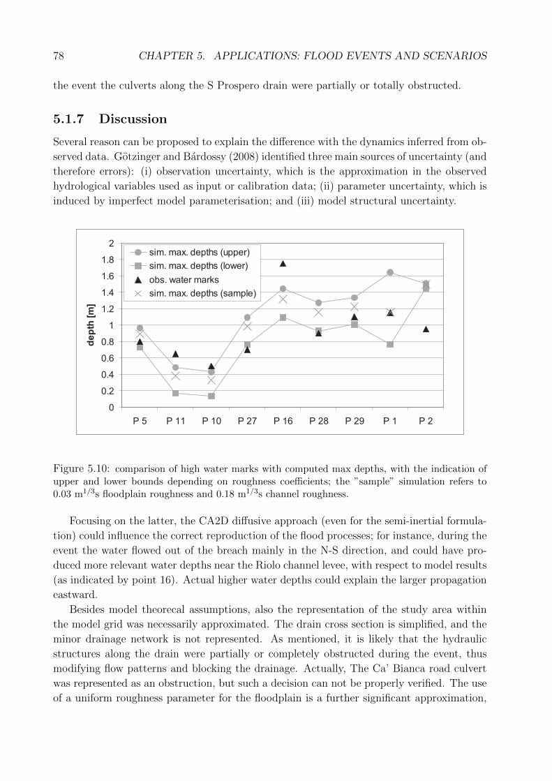
78 CHAPTER 5. APPLICATIONS: FLOOD EVENTS AND SCENARIOS
the event the culverts along the S Prospero drain were partially or totally obstructed.
5.1.7 Discussion
Several reason can be proposed to explain the difference with the dynamics inferred from ob-
served data. Gotzinger and Bardossy (2008) identified three main sources of uncertainty (and
therefore errors): (i) observation uncertainty, which is the approximation in the observed
hydrological variables used as input or calibration data; (ii) parameter uncertainty, which is
induced by imperfect model parameterisation; and (iii) model structural uncertainty.
0
0.2
0.4
0.6
0.8
1
1.2
1.4
1.6
1.8
2
P 5 P 11 P 10 P 27 P 16 P 28 P 29 P 1 P 2
de
pth
[m]
sim. max. depths (upper)
sim. max. depths (lower)
obs. water marks
sim. max. depths (sample)
Figure 5.10: comparison of high water marks with computed max depths, with the indication ofupper and lower bounds depending on roughness coefficients; the ”sample” simulation refers to0.03 m1/3s floodplain roughness and 0.18 m1/3s channel roughness.
Focusing on the latter, the CA2D diffusive approach (even for the semi-inertial formula-
tion) could influence the correct reproduction of the flood processes; for instance, during the
event the water flowed out of the breach mainly in the N-S direction, and could have pro-
duced more relevant water depths near the Riolo channel levee, with respect to model results
(as indicated by point 16). Actual higher water depths could explain the larger propagation
eastward.
Besides model theorecal assumptions, also the representation of the study area within
the model grid was necessarily approximated. The drain cross section is simplified, and the
minor drainage network is not represented. As mentioned, it is likely that the hydraulic
structures along the drain were partially or completely obstructed during the event, thus
modifying flow patterns and blocking the drainage. Actually, The Ca’ Bianca road culvert
was represented as an obstruction, but such a decision can not be properly verified. The use
of a uniform roughness parameter for the floodplain is a further significant approximation,
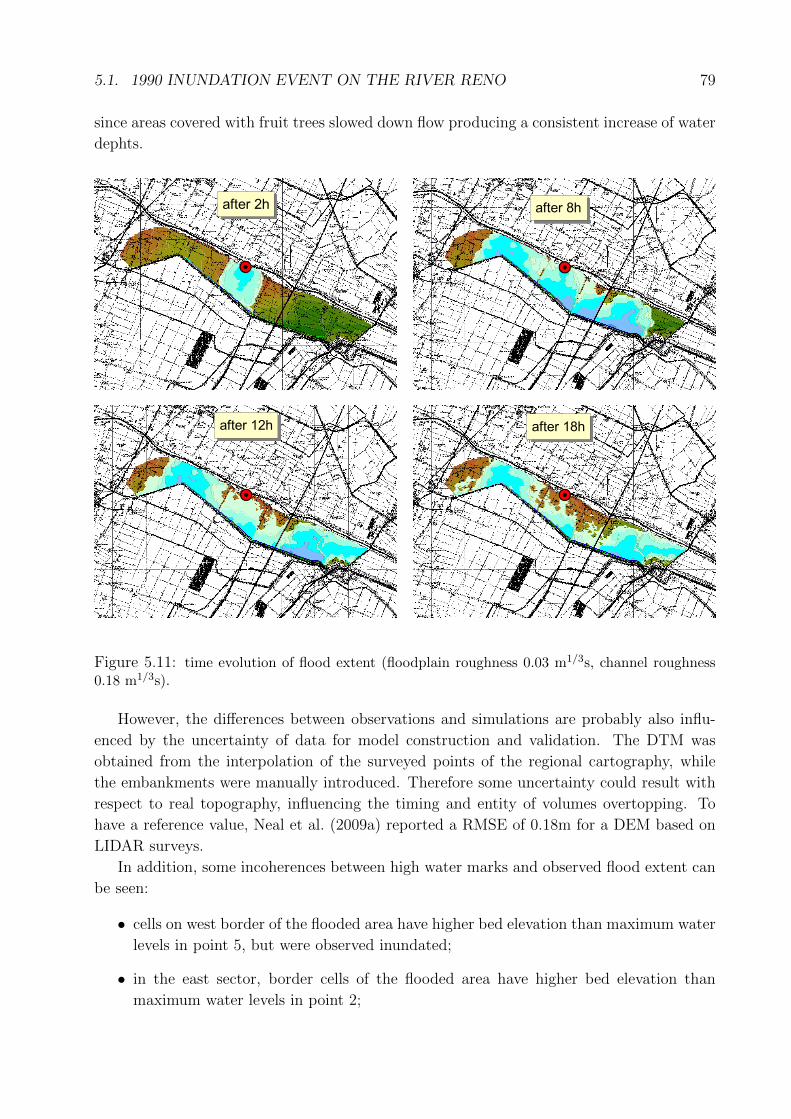
5.1. 1990 INUNDATION EVENT ON THE RIVER RENO 79
since areas covered with fruit trees slowed down flow producing a consistent increase of water
dephts.
Figure 5.11: time evolution of flood extent (floodplain roughness 0.03 m1/3s, channel roughness0.18 m1/3s).
However, the differences between observations and simulations are probably also influ-
enced by the uncertainty of data for model construction and validation. The DTM was
obtained from the interpolation of the surveyed points of the regional cartography, while
the embankments were manually introduced. Therefore some uncertainty could result with
respect to real topography, influencing the timing and entity of volumes overtopping. To
have a reference value, Neal et al. (2009a) reported a RMSE of 0.18m for a DEM based on
LIDAR surveys.
In addition, some incoherences between high water marks and observed flood extent can
be seen:
• cells on west border of the flooded area have higher bed elevation than maximum water
levels in point 5, but were observed inundated;
• in the east sector, border cells of the flooded area have higher bed elevation than
maximum water levels in point 2;
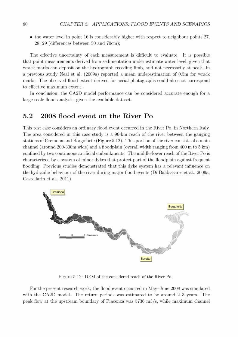
80 CHAPTER 5. APPLICATIONS: FLOOD EVENTS AND SCENARIOS
• the water level in point 16 is considerably higher with respect to neighbour points 27,
28, 29 (differences between 50 and 70cm);
The effective uncertainty of each measurement is difficult to evaluate. It is possible
that point measurements derived from sedimentation under estimate water level, given that
wrack marks can deposit on the hydrograph receding limb, and not necessarily at peak. In
a previous study Neal et al. (2009a) reported a mean underestimation of 0.5m for wrack
marks. The observed flood extent derived for aerial photographs could also not correspond
to effective maximum extent.
In conclusion, the CA2D model performance can be considered accurate enough for a
large scale flood analysis, given the available dataset.
5.2 2008 flood event on the River Po
This test case considers an ordinary flood event occurred in the River Po, in Northern Italy.
The area considered in this case study is a 96-km reach of the river between the gauging
stations of Cremona and Borgoforte (Figure 5.12). This portion of the river consists of a main
channel (around 200-300m wide) and a floodplain (overall width ranging from 400 m to 5 km)
confined by two continuous artificial embankments. The middle-lower reach of the River Po is
characterized by a system of minor dykes that protect part of the floodplain against frequent
flooding. Previous studies demonstrated that this dyke system has a relevant influence on
the hydraulic behaviour of the river during major flood events (Di Baldassarre et al., 2009a;
Castellarin et al., 2011).
Figure 5.12: DEM of the considered reach of the River Po.
For the present research work, the flood event occurred in May–June 2008 was simulated
with the CA2D model. The return periods was estimated to be around 2–3 years. The
peak flow at the upstream boundary of Piacenza was 5736 m3/s, while maximum channel
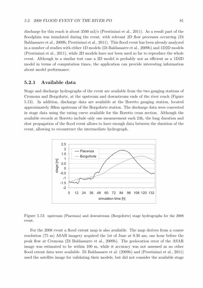
5.2. 2008 FLOOD EVENT ON THE RIVER PO 81
discharge for this reach is about 3500 m3/s (Prestininzi et al., 2011). As a result part of the
floodplain was inundated during the event, with relevant 2D flow processes occurring (Di
Baldassarre et al., 2009b; Prestininzi et al., 2011). This flood event has been already analyzed
in a number of studies with either 1D models (Di Baldassarre et al., 2009b) and 1D2D models
(Prestininzi et al., 2011), while 2D models have not been used so far to reproduce the whole
event. Although in a similar test case a 2D model is probably not as efficient as a 1D2D
model in terms of computation times, the application can provide interesting information
about model performance.
5.2.1 Available data
Stage and discharge hydrographs of the event are available from the two gauging stations of
Cremona and Borgoforte, at the upstream and downstream ends of the river reach (Figure
5.13). In addition, discharge data are available at the Boretto gauging station, located
approximately 30km upstream of the Borgoforte station. The discharge data were converted
in stage data using the rating curve available for the Boretto cross section. Although the
available records at Boretto include only one measurement each 24h, the long duration and
slow propagation of the flood event allows to have enough data between the duration of the
event, allowing to reconstruct the intermediate hydrograph.
-2
-1.5
-1
-0.5
0
0.5
1
1.5
2
2.5
0 12 24 36 48 60 72 84 96 108 120 132
simulation time [h]
sta
ge
[m]
Piacenza
Borgoforte
Figure 5.13: upstream (Piacenza) and downstream (Borgoforte) stage hydrographs for the 2008event.
For the 2008 event a flood extent map is also available. The map derives from a coarse
resolution (75 m) ASAR imagery acquired the 1st of June at 9.30 am, one hour before the
peak flow at Cremona (Di Baldassarre et al., 2009b). The geolocation error of the ASAR
image was estimated to be within 100 m, while it accuracy was not assessed as no other
flood extent data were available. Di Baldassarre et al. (2009b) and (Prestininzi et al., 2011)
used the satellite image for validating their models, but did not consider the available stage
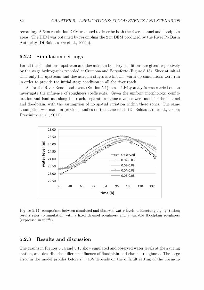
82 CHAPTER 5. APPLICATIONS: FLOOD EVENTS AND SCENARIOS
recording. A 64m resolution DEM was used to describe both the river channel and floodplain
areas. The DEM was obtained by resampling the 2 m DEM produced by the River Po Basin
Authority (Di Baldassarre et al., 2009b).
5.2.2 Simulation settings
For all the simulations, upstream and downstream boudary conditions are given respectively
by the stage hydrographs recorded at Cremona and Borgoforte (Figure 5.13). Since at initial
time only the upstream and downstream stages are known, warm-up simulations were run
in order to provide the initial stage condition in all the river reach.
As for the River Reno flood event (Section 5.1), a sensitivity analysis was carried out to
investigate the influence of roughness coefficients. Given the uniform morphologic config-
uration and land use along the reach, separate roughness values were used for the channel
and floodplain, with the assumption of no spatial variation within these zones. The same
assumption was made in previous studies on the same reach (Di Baldassarre et al., 2009b;
Prestininzi et al., 2011).
22.50
23.00
23.50
24.00
24.50
25.00
25.50
26.00
36 48 60 72 84 96 108 120 132
time (h)
wa
ter
lev
el
(m)
Observed
0.02-0.08
0.03-0.08
0.04-0.08
0.05-0.08
Figure 5.14: comparison between simulated and observed water levels at Boretto gauging station;results refer to simulation with a fixed channel roughness and a variable floodplain roughness(expressed in m1/3s).
5.2.3 Results and discussion
The graphs in Figures 5.14 and 5.15 show simulated and observed water levels at the gauging
station, and describe the different influence of floodplain and channel roughness. The large
error in the model profiles before t = 48h depends on the difficult setting of the warm-up
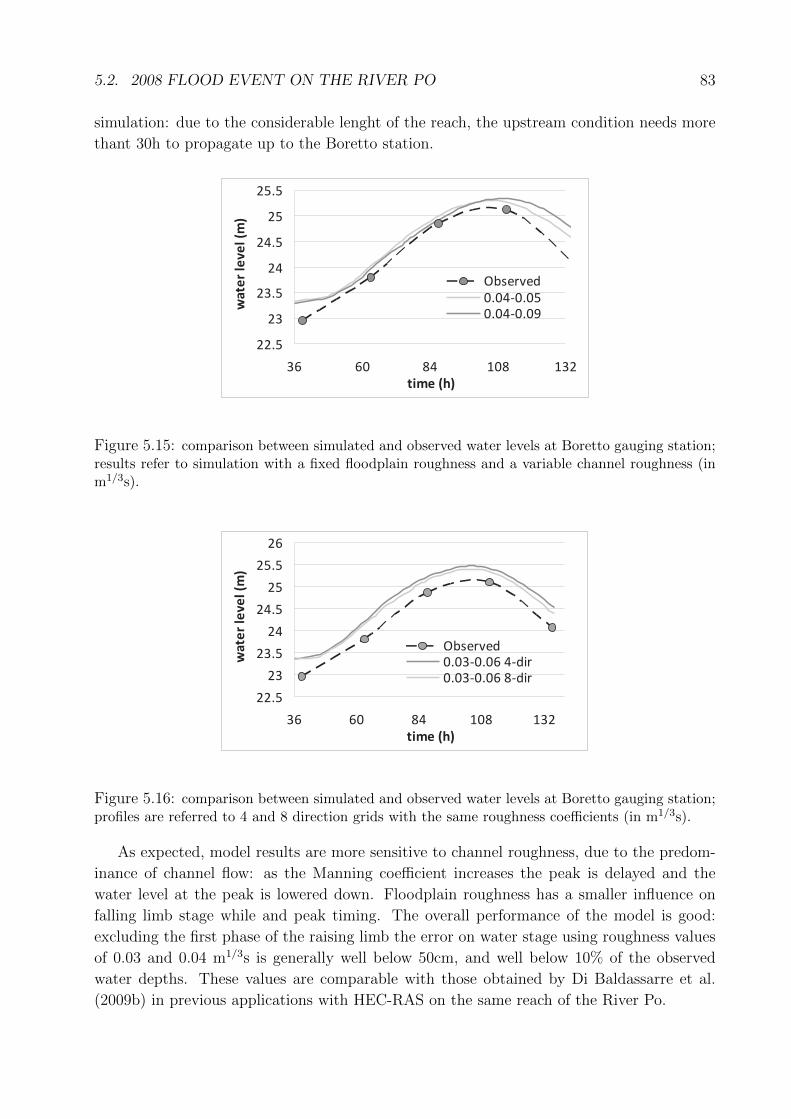
5.2. 2008 FLOOD EVENT ON THE RIVER PO 83
simulation: due to the considerable lenght of the reach, the upstream condition needs more
thant 30h to propagate up to the Boretto station.
22.5
23
23.5
24
24.5
25
25.5
36 60 84 108 132
time (h)
wa
ter
lev
el
(m)
Observed
0.04-0.05
0.04-0.09
Figure 5.15: comparison between simulated and observed water levels at Boretto gauging station;results refer to simulation with a fixed floodplain roughness and a variable channel roughness (inm1/3s).
22.5
23
23.5
24
24.5
25
25.5
26
36 60 84 108 132
time (h)
wa
ter
lev
el
(m)
Observed
0.03-0.06 4-dir
0.03-0.06 8-dir
Figure 5.16: comparison between simulated and observed water levels at Boretto gauging station;profiles are referred to 4 and 8 direction grids with the same roughness coefficients (in m1/3s).
As expected, model results are more sensitive to channel roughness, due to the predom-
inance of channel flow: as the Manning coefficient increases the peak is delayed and the
water level at the peak is lowered down. Floodplain roughness has a smaller influence on
falling limb stage while and peak timing. The overall performance of the model is good:
excluding the first phase of the raising limb the error on water stage using roughness values
of 0.03 and 0.04 m1/3s is generally well below 50cm, and well below 10% of the observed
water depths. These values are comparable with those obtained by Di Baldassarre et al.
(2009b) in previous applications with HEC-RAS on the same reach of the River Po.
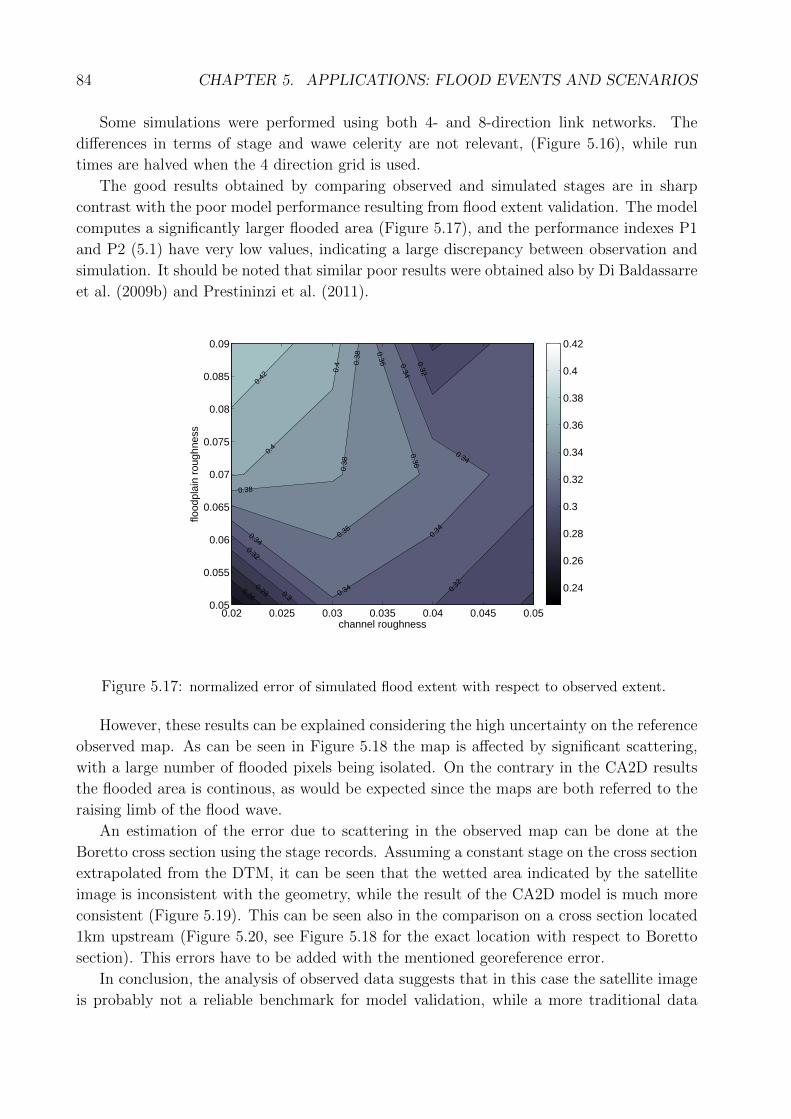
84 CHAPTER 5. APPLICATIONS: FLOOD EVENTS AND SCENARIOS
Some simulations were performed using both 4- and 8-direction link networks. The
differences in terms of stage and wawe celerity are not relevant, (Figure 5.16), while run
times are halved when the 4 direction grid is used.
The good results obtained by comparing observed and simulated stages are in sharp
contrast with the poor model performance resulting from flood extent validation. The model
computes a significantly larger flooded area (Figure 5.17), and the performance indexes P1
and P2 (5.1) have very low values, indicating a large discrepancy between observation and
simulation. It should be noted that similar poor results were obtained also by Di Baldassarre
et al. (2009b) and Prestininzi et al. (2011).
0.26
0.28 0.3
0.32
0.32
0.32
0.34
0.34
0.34
0.34
0.34
0.36
0.36
0.36
0.38
0.38
0.38
0.4
0.4
0.42
channel roughness
flood
plai
n ro
ughn
ess
0.02 0.025 0.03 0.035 0.04 0.045 0.050.05
0.055
0.06
0.065
0.07
0.075
0.08
0.085
0.09
0.24
0.26
0.28
0.3
0.32
0.34
0.36
0.38
0.4
0.42
Figure 5.17: normalized error of simulated flood extent with respect to observed extent.
However, these results can be explained considering the high uncertainty on the reference
observed map. As can be seen in Figure 5.18 the map is affected by significant scattering,
with a large number of flooded pixels being isolated. On the contrary in the CA2D results
the flooded area is continous, as would be expected since the maps are both referred to the
raising limb of the flood wave.
An estimation of the error due to scattering in the observed map can be done at the
Boretto cross section using the stage records. Assuming a constant stage on the cross section
extrapolated from the DTM, it can be seen that the wetted area indicated by the satellite
image is inconsistent with the geometry, while the result of the CA2D model is much more
consistent (Figure 5.19). This can be seen also in the comparison on a cross section located
1km upstream (Figure 5.20, see Figure 5.18 for the exact location with respect to Boretto
section). This errors have to be added with the mentioned georeference error.
In conclusion, the analysis of observed data suggests that in this case the satellite image
is probably not a reliable benchmark for model validation, while a more traditional data
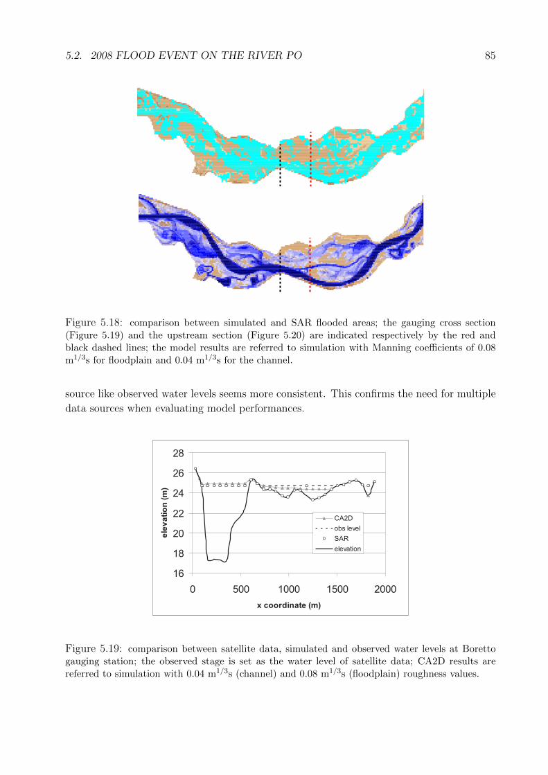
5.2. 2008 FLOOD EVENT ON THE RIVER PO 85
Figure 5.18: comparison between simulated and SAR flooded areas; the gauging cross section(Figure 5.19) and the upstream section (Figure 5.20) are indicated respectively by the red andblack dashed lines; the model results are referred to simulation with Manning coefficients of 0.08m1/3s for floodplain and 0.04 m1/3s for the channel.
source like observed water levels seems more consistent. This confirms the need for multiple
data sources when evaluating model performances.
16
18
20
22
24
26
28
0 500 1000 1500 2000
x coordinate (m)
ele
va
tio
n(m
)
CA2D
obs level
SAR
elevation
Figure 5.19: comparison between satellite data, simulated and observed water levels at Borettogauging station; the observed stage is set as the water level of satellite data; CA2D results arereferred to simulation with 0.04 m1/3s (channel) and 0.08 m1/3s (floodplain) roughness values.

86 CHAPTER 5. APPLICATIONS: FLOOD EVENTS AND SCENARIOS
16
18
20
22
24
26
28
0 500 1000
x coordinate (m)
ele
va
tio
n(m
)on
CA2D
SAR
elevation
Figure 5.20: comparison between satellite data and simulated water levels 1km ustream of Borettogauging station (Figure 5.18); CA2D results are referred to simulation with 0.04 m1/3s (channel)and 0.08 m1/3s (floodplain) roughness values.
5.3 Flood risk mapping on the River Ubaye
The case study described in this section is part of the research work carried out for the
European project KULTURisk (www.kulturisk.eu). The area is located in the upper part
of the valley of the River Ubaye, in the French Alps. The study area includes the river bed
and the sorrounding floodplain, which is partly occupied by the urban area of Barcelonnette
(Figure 5.21).
The river is mainly characterized by a large unconfined gravel bed, typical of mountain
rivers. However, near the urban area the river is canalized and constrained by embankments
in a narrow trapezoidal artificial section. Therefore the test area includes both the artificial
bed reach and portions of bed in natural conditions upstream and downstream.
Barcelonnette was affected by a major flood event in 1957, that caused the flooding of
a significant portion of the village. After that event, the existing system of dykes were
reinforced and heightened. In 2008, another significant flood event occurred in the River
Ubaye. The water remained within the river bed, but the recorded water levels were the
highest since the 1957 flood. This is the event that has been simulated with the CA2D
model.
Although 1D flow routing is not an usual application for a 2D model, this case provides a
good benchmark for testing the ability of CA2D to reproduce 1D flow over a steep slope, with
alternance of subcritical and supercritical flow and considerable changes of river cross section.
Given the presence of dykes, in this case the use of a 2D–based model could be advisable to
simulate both in–bed and floodplain flow and the consequent complex interaction.
It is worth noting that most applications of 2D models in literature are carried out on
flat floodplain areas, especially when mixed 1D-2D flows are simulated. Applications to
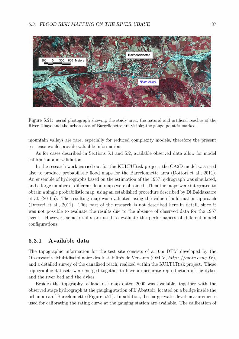
5.3. FLOOD RISK MAPPING ON THE RIVER UBAYE 87
Figure 5.21: aerial photograph showing the study area; the natural and artificial reaches of theRiver Ubaye and the urban area of Barcellonette are visible; the gauge point is marked.
mountain valleys are rare, especially for reduced complexity models, therefore the present
test case would provide valuable information.
As for cases described in Sections 5.1 and 5.2, available observed data allow for model
calibration and validation.
In the research work carried out for the KULTURisk project, the CA2D model was used
also to produce probabilistic flood maps for the Barcelonnette area (Dottori et al., 2011).
An ensemble of hydrographs based on the estimation of the 1957 hydrograph was simulated,
and a large number of different flood maps were obtained. Then the maps were integrated to
obtain a single probabilistic map, using an established procedure described by Di Baldassarre
et al. (2010b). The resulting map was evaluated using the value of information approach
(Dottori et al., 2011). This part of the research is not described here in detail, since it
was not possible to evaluate the results due to the absence of observed data for the 1957
event. However, some results are used to evaluate the performances of different model
configurations.
5.3.1 Available data
The topographic information for the test site consists of a 10m DTM developed by the
Observatoire Multidisciplinaire des Instabilites de Versants (OMIV, http : //omiv.osug.fr),
and a detailed survey of the canalized reach, realized within the KULTURisk project. These
topographic datasets were merged together to have an accurate reproduction of the dykes
and the river bed and the dykes.
Besides the topgraphy, a land use map dated 2000 was available, together with the
observed stage hydrograph at the gauging station of L’Abattoir, located on a bridge inside the
urban area of Barcelonnette (Figure 5.21). In addition, discharge–water level measurements
used for calibrating the rating curve at the gauging station are available. The calibration of
88 CHAPTER 5. APPLICATIONS: FLOOD EVENTS AND SCENARIOS
the rating curve was performed the year before the considered 2008 event.
5.3.2 Simulation settings
In order to obtain the upstream boundary condition for the simulation, the available stage
hydrograph was converted into a discharge hydrograph using the rating curve, and used
as the upstream condition. Although such operation is not theoretically correct, it can be
considered acceptable for the present case. The bed slope is steep in all the considered
reach (more than 0.5%), and this means that the flow condition can be considered almost
kinematic, and the flood wave should travel along the reach without significant attenuation.
Therefore, the hydrograph at the Abattoir cross section was simply anticipated by estimating
the time of delay between the upstream and the gauging station cross sections. It also worth
noting that due to the kinematic condition the rating curve should not be affected by a
significant hysteresis.
The Manning coefficient for the canalized reach was estimated by applying the uniform
flow formula to the available coupled measurements of stage and discharge. For water depths
over 2m, a value of 0.037 m1/3s was estimated. For the natural portions of the reach a value
of 0.05 m1/3s was set. Although effective roughness can be different when evaluated in
different flow conditions (Horritt, 2002; Hunter et al., 2007), given the regularized section
it is reasonable to assume a constant roughness value for high discharge rates. Given these
friction coefficients, some simulations with simple wave hydrographs were used to estimate
the wave travel time between the upstream boundary and the gauging station, resulting in
1 hour delay. The calibration showed also that the assumption of large rectangular section
within the model is consistent in this case, with a depth/width ratio below 0.1.
Since this case study deals with a 1D flow over a narrow channel with considerable
changes of direction, the simulations have been performed using both 4 direction and 8
direction link netwoks, in order to test the reliability of each grid configuration under such
flow conditions.
A critical flow was set as downstream boundary condition. Since the area of interest is
limited to the canalized reach, and given the steep slopes, such a choice do not influence
model results.
5.3.3 Results
Figure 5.22 shows the comparison between simulated and observed water dephts at the
gauging station using both 4- and 8-direction grids. As can be seen, the model computed
slightly lower water depths, which can be due to the wave attenuation. Attenuation is higher
in 4 direction than in 8 direction grid, whereas the hydrograph profile is well reproduced by
both link networks.
Figures 5.23, 5.24 and 5.25 illustrate the model results in the upstream part of the study
reach, in terms of maximum water depth, velocity and Froude number. It can be seen that
where the river bed narrows a transition from subcritical to supercritical condition occurs.
As discussed in Section 4.5, the CA2D model is not able to reproduce the exact profile of
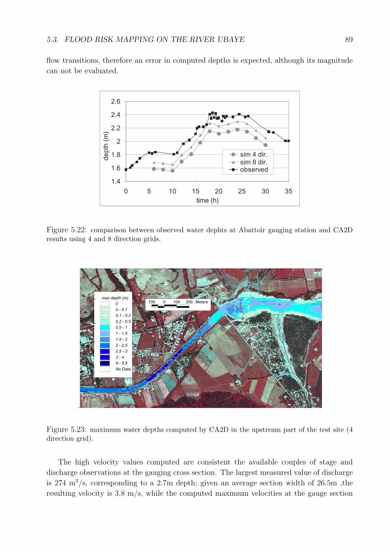
5.3. FLOOD RISK MAPPING ON THE RIVER UBAYE 89
flow transitions, therefore an error in computed depths is expected, although its magnitude
can not be evaluated.
1.4
1.6
1.8
2
2.2
2.4
2.6
0 5 10 15 20 25 30 35
time (h)
de
pth
(m)
sim 4 dir.sim 8 dir.observed
Figure 5.22: comparison between observed water dephts at Abattoir gauging station and CA2Dresults using 4 and 8 direction grids.
.
Figure 5.23: maximum water depths computed by CA2D in the upstream part of the test site (4direction grid).
The high velocity values computed are consistent the available couples of stage and
discharge observations at the gauging cross section. The largest measured value of discharge
is 274 m3/s, corresponding to a 2.7m depth; given an average section width of 26.5m ,the
resulting velocity is 3.8 m/s, while the computed maximum velocities at the gauge section
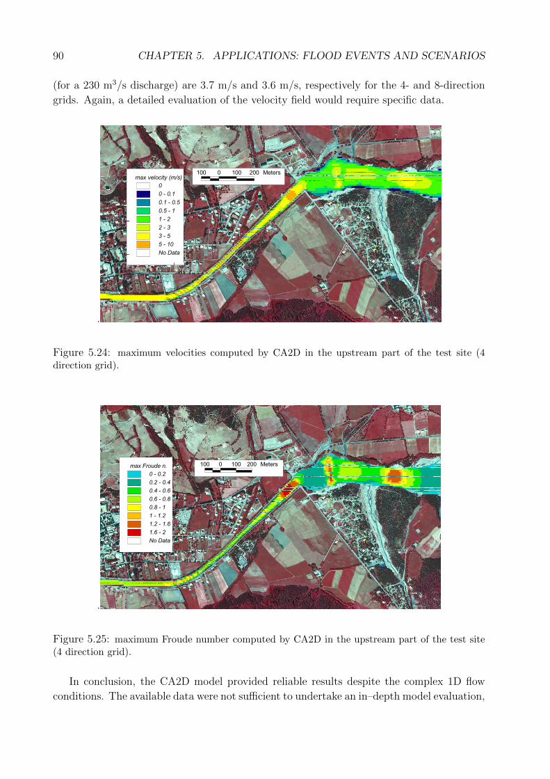
90 CHAPTER 5. APPLICATIONS: FLOOD EVENTS AND SCENARIOS
(for a 230 m3/s discharge) are 3.7 m/s and 3.6 m/s, respectively for the 4- and 8-direction
grids. Again, a detailed evaluation of the velocity field would require specific data.
.
Figure 5.24: maximum velocities computed by CA2D in the upstream part of the test site (4direction grid).
.
Figure 5.25: maximum Froude number computed by CA2D in the upstream part of the test site(4 direction grid).
In conclusion, the CA2D model provided reliable results despite the complex 1D flow
conditions. The available data were not sufficient to undertake an in–depth model evaluation,
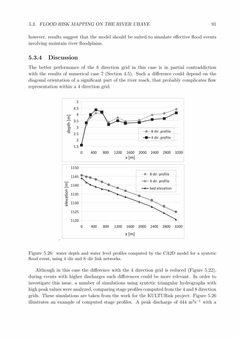
5.3. FLOOD RISK MAPPING ON THE RIVER UBAYE 91
however, results suggest that the model should be suited to simulate effective flood events
involving mointain river floodplains.
5.3.4 Discussion
The better performance of the 8 direction grid in this case is in partial contraddiction
with the results of numerical case 7 (Section 4.5). Such a difference could depend on the
diagonal orientation of a significant part of the river reach, that probably complicates flow
representation within a 4 direction grid.
.
1120
1125
1130
1135
1140
1145
1150
0 400 800 1200 1600 2000 2400 2800 3200
x [m]
ele
va
tio
n[m
]
8 dir. profile
4 dir. profile
bed elevation
1.5
2
2.5
3
3.5
4
4.5
5
0 400 800 1200 1600 2000 2400 2800 3200
x [m]
de
pth
[m]
8 dir. profile
4 dir. profile
Figure 5.26: water depth and water level profiles computed by the CA2D model for a synteticflood event, using 4–dir and 8–dir link networks.
Although in this case the difference with the 4 direction grid is reduced (Figure 5.22),
during events with higher discharges such differences could be more relevant. In order to
investigate this issue, a number of simulations using syntetic triangular hydrographs with
high peak values were analyzed, comparing stage profiles computed from the 4 and 8 direction
grids. These simulations are taken from the work for the KULTURisk project. Figure 5.26
illustrates an example of computed stage profiles. A peak discharge of 444 m3s−1 with a
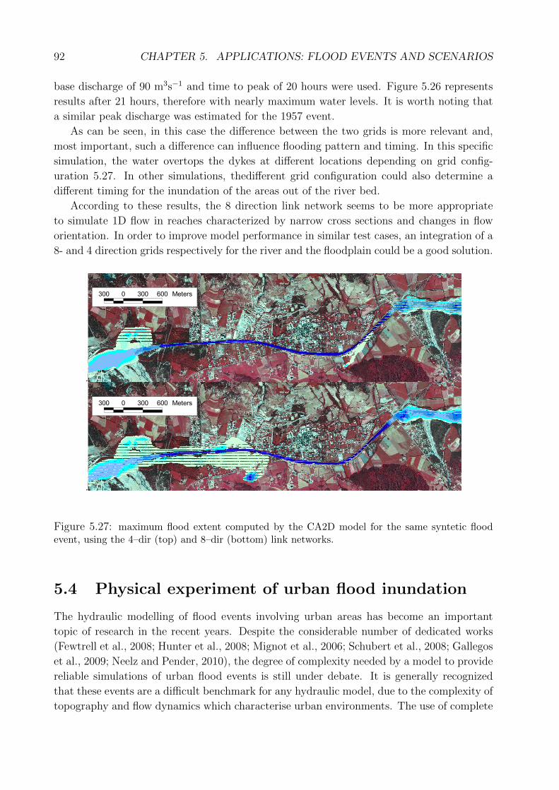
92 CHAPTER 5. APPLICATIONS: FLOOD EVENTS AND SCENARIOS
base discharge of 90 m3s−1 and time to peak of 20 hours were used. Figure 5.26 represents
results after 21 hours, therefore with nearly maximum water levels. It is worth noting that
a similar peak discharge was estimated for the 1957 event.
As can be seen, in this case the difference between the two grids is more relevant and,
most important, such a difference can influence flooding pattern and timing. In this specific
simulation, the water overtops the dykes at different locations depending on grid config-
uration 5.27. In other simulations, thedifferent grid configuration could also determine a
different timing for the inundation of the areas out of the river bed.
According to these results, the 8 direction link network seems to be more appropriate
to simulate 1D flow in reaches characterized by narrow cross sections and changes in flow
orientation. In order to improve model performance in similar test cases, an integration of a
8- and 4 direction grids respectively for the river and the floodplain could be a good solution.
.
.
Figure 5.27: maximum flood extent computed by the CA2D model for the same syntetic floodevent, using the 4–dir (top) and 8–dir (bottom) link networks.
5.4 Physical experiment of urban flood inundation
The hydraulic modelling of flood events involving urban areas has become an important
topic of research in the recent years. Despite the considerable number of dedicated works
(Fewtrell et al., 2008; Hunter et al., 2008; Mignot et al., 2006; Schubert et al., 2008; Gallegos
et al., 2009; Neelz and Pender, 2010), the degree of complexity needed by a model to provide
reliable simulations of urban flood events is still under debate. It is generally recognized
that these events are a difficult benchmark for any hydraulic model, due to the complexity of
topography and flow dynamics which characterise urban environments. The use of complete
5.4. PHYSICAL EXPERIMENT OF URBAN FLOOD INUNDATION 93
2D models based on full SWE should be recommendable (Cunge, 2003; El Kadi et al., 2009),
but in most of the cases the scarcity of observed data prevents an adequate evaluation
(Hunter et al., 2007; Neal et al., 2009a). As a consequence, many research works used
reduced complexity models for simulating urban flood events, exploiting their simplicity of
development and application and their low data requirement (Yu and Lane, 2006a; Hunter
et al., 2008; Fewtrell et al., 2011).
However, caution should be used. Reduced complexity models are designed to simulate
only part of the flow processes, therefore risks of inappropriate application are likely to
arise. Indeed, detailed analyses of the effective ability and limitation of simplified models in
reproducing floods processes are still rare, especially for urban environments.
Hunter et al. (2008) compared a number of 2d models of varying complexity in a single
urban flood scenario, and observed that the overall performance of reduced complexity mod-
els were comparable to more complex models. Prestininzi (2008) used a simplified 2D model,
based on parabolic equations, to reproduce an experiment carried out in a physical model,
observing a generally good performance. Neelz and Pender (2010) performed a detailed ana-
lyses of different 2d models in a number of numerical cases, including dam break physical
experiments.
Considering this framework, the use of laboratory experiment data can be seen as a good
solution for evaluating reduced complexity models. Experimental data allow the possibility
to test model performances in detail, since flow conditions may be accurately controlled
and reliable data for model calibration and evaluation are available Sanders (2008); El Kadi
et al. (2009). Therefore, in this test case, the CA2D model is used to simulate different
experiments of urban flood, carried out using a physical model.
5.4.1 Case study description
The description of present case is taken from Dottori and Todini (2012). For reasons of
conciseness, not all the simulations performed in that paper are here described.
The model has been tested by reproducing the results of a number of experiments, in-
cluded in the IMPACT European project (Investigation of extreMe flood Processes And
unCerTainty, Alcrudo (2004)). These experiments are part of a broader study of flood
propagation in urban areas, and have been described in detail by Testa et al. (2007). In the
experiments, a series of concrete blocks was placed in an instrumented physical model of a
short reach of the Alpine Toce River at a 1:100 scale, to simulate the ooding of an urban
district. Two building configurations were tested: either aligned in a regular pattern, or
placed in checker board (staggered) layout. Figure 5.28 shows the aligned and staggered
layouts.
Flooding of the model is achieved by rapidly raising the water level in a feed tank located
at the upstream end of the model. Different hydrographs were used in the experiments; this
paper only includes the results for low and medium hydrographs described by Testa et al.
(2007). In Figure 5.29 the hydrographs are reported. The average terrain slope is between
2% and 3%, with local values in the channel up to 20%. Time series of water depth at

94 CHAPTER 5. APPLICATIONS: FLOOD EVENTS AND SCENARIOS
!"
#!$ %
!"
#!$ %
Figure 5.28: digital elevation models of the physical model with the position of gauge points. Thealigned (left) and staggered (right) building layouts are represented.
different locations were recorded for all the configurations of the model city, surrounding
terrain and flooding conditions. These data provide exhaustive information on spatial and
temporal flow dynamics and therefore allow a detailed evaluation of the model performance.
Figure 5.29: discharge hydrographs used in the simulations.
Testa et al. (2007) provided a general description of flow processes. In all the config-
urations, the presence of the urban district produced a strong hydraulic jump immediately
upstream of the buildings, and a complex ow pattern inside the urban district. Differences
in water depth readings at various locations among the buildings arose from the complexity
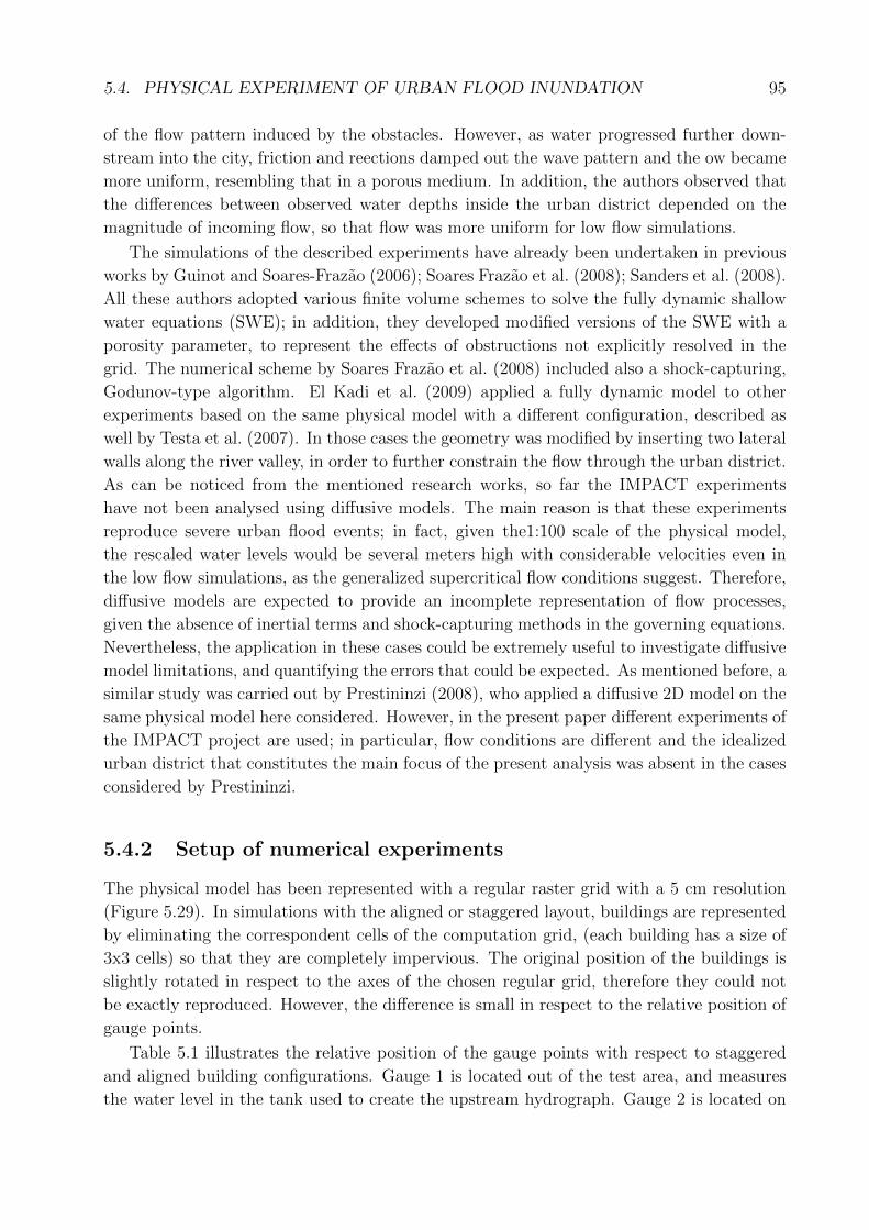
5.4. PHYSICAL EXPERIMENT OF URBAN FLOOD INUNDATION 95
of the flow pattern induced by the obstacles. However, as water progressed further down-
stream into the city, friction and reections damped out the wave pattern and the ow became
more uniform, resembling that in a porous medium. In addition, the authors observed that
the differences between observed water depths inside the urban district depended on the
magnitude of incoming flow, so that flow was more uniform for low flow simulations.
The simulations of the described experiments have already been undertaken in previous
works by Guinot and Soares-Frazao (2006); Soares Frazao et al. (2008); Sanders et al. (2008).
All these authors adopted various finite volume schemes to solve the fully dynamic shallow
water equations (SWE); in addition, they developed modified versions of the SWE with a
porosity parameter, to represent the effects of obstructions not explicitly resolved in the
grid. The numerical scheme by Soares Frazao et al. (2008) included also a shock-capturing,
Godunov-type algorithm. El Kadi et al. (2009) applied a fully dynamic model to other
experiments based on the same physical model with a different configuration, described as
well by Testa et al. (2007). In those cases the geometry was modified by inserting two lateral
walls along the river valley, in order to further constrain the flow through the urban district.
As can be noticed from the mentioned research works, so far the IMPACT experiments
have not been analysed using diffusive models. The main reason is that these experiments
reproduce severe urban flood events; in fact, given the1:100 scale of the physical model,
the rescaled water levels would be several meters high with considerable velocities even in
the low flow simulations, as the generalized supercritical flow conditions suggest. Therefore,
diffusive models are expected to provide an incomplete representation of flow processes,
given the absence of inertial terms and shock-capturing methods in the governing equations.
Nevertheless, the application in these cases could be extremely useful to investigate diffusive
model limitations, and quantifying the errors that could be expected. As mentioned before, a
similar study was carried out by Prestininzi (2008), who applied a diffusive 2D model on the
same physical model here considered. However, in the present paper different experiments of
the IMPACT project are used; in particular, flow conditions are different and the idealized
urban district that constitutes the main focus of the present analysis was absent in the cases
considered by Prestininzi.
5.4.2 Setup of numerical experiments
The physical model has been represented with a regular raster grid with a 5 cm resolution
(Figure 5.29). In simulations with the aligned or staggered layout, buildings are represented
by eliminating the correspondent cells of the computation grid, (each building has a size of
3x3 cells) so that they are completely impervious. The original position of the buildings is
slightly rotated in respect to the axes of the chosen regular grid, therefore they could not
be exactly reproduced. However, the difference is small in respect to the relative position of
gauge points.
Table 5.1 illustrates the relative position of the gauge points with respect to staggered
and aligned building configurations. Gauge 1 is located out of the test area, and measures
the water level in the tank used to create the upstream hydrograph. Gauge 2 is located on
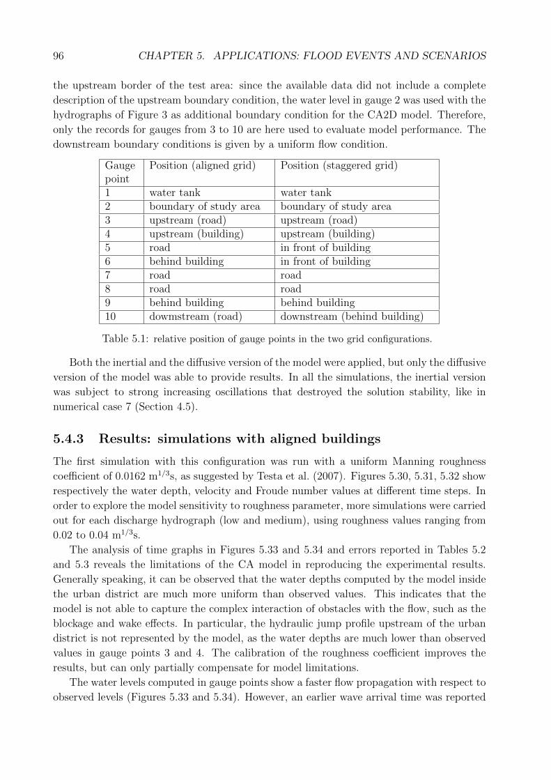
96 CHAPTER 5. APPLICATIONS: FLOOD EVENTS AND SCENARIOS
the upstream border of the test area: since the available data did not include a complete
description of the upstream boundary condition, the water level in gauge 2 was used with the
hydrographs of Figure 3 as additional boundary condition for the CA2D model. Therefore,
only the records for gauges from 3 to 10 are here used to evaluate model performance. The
downstream boundary conditions is given by a uniform flow condition.
Gaugepoint
Position (aligned grid) Position (staggered grid)
1 water tank water tank2 boundary of study area boundary of study area3 upstream (road) upstream (road)4 upstream (building) upstream (building)5 road in front of building6 behind building in front of building7 road road8 road road9 behind building behind building10 dowmstream (road) downstream (behind building)
Table 5.1: relative position of gauge points in the two grid configurations.
Both the inertial and the diffusive version of the model were applied, but only the diffusive
version of the model was able to provide results. In all the simulations, the inertial version
was subject to strong increasing oscillations that destroyed the solution stability, like in
numerical case 7 (Section 4.5).
5.4.3 Results: simulations with aligned buildings
The first simulation with this configuration was run with a uniform Manning roughness
coefficient of 0.0162 m1/3s, as suggested by Testa et al. (2007). Figures 5.30, 5.31, 5.32 show
respectively the water depth, velocity and Froude number values at different time steps. In
order to explore the model sensitivity to roughness parameter, more simulations were carried
out for each discharge hydrograph (low and medium), using roughness values ranging from
0.02 to 0.04 m1/3s.
The analysis of time graphs in Figures 5.33 and 5.34 and errors reported in Tables 5.2
and 5.3 reveals the limitations of the CA model in reproducing the experimental results.
Generally speaking, it can be observed that the water depths computed by the model inside
the urban district are much more uniform than observed values. This indicates that the
model is not able to capture the complex interaction of obstacles with the flow, such as the
blockage and wake effects. In particular, the hydraulic jump profile upstream of the urban
district is not represented by the model, as the water depths are much lower than observed
values in gauge points 3 and 4. The calibration of the roughness coefficient improves the
results, but can only partially compensate for model limitations.
The water levels computed in gauge points show a faster flow propagation with respect to
observed levels (Figures 5.33 and 5.34). However, an earlier wave arrival time was reported
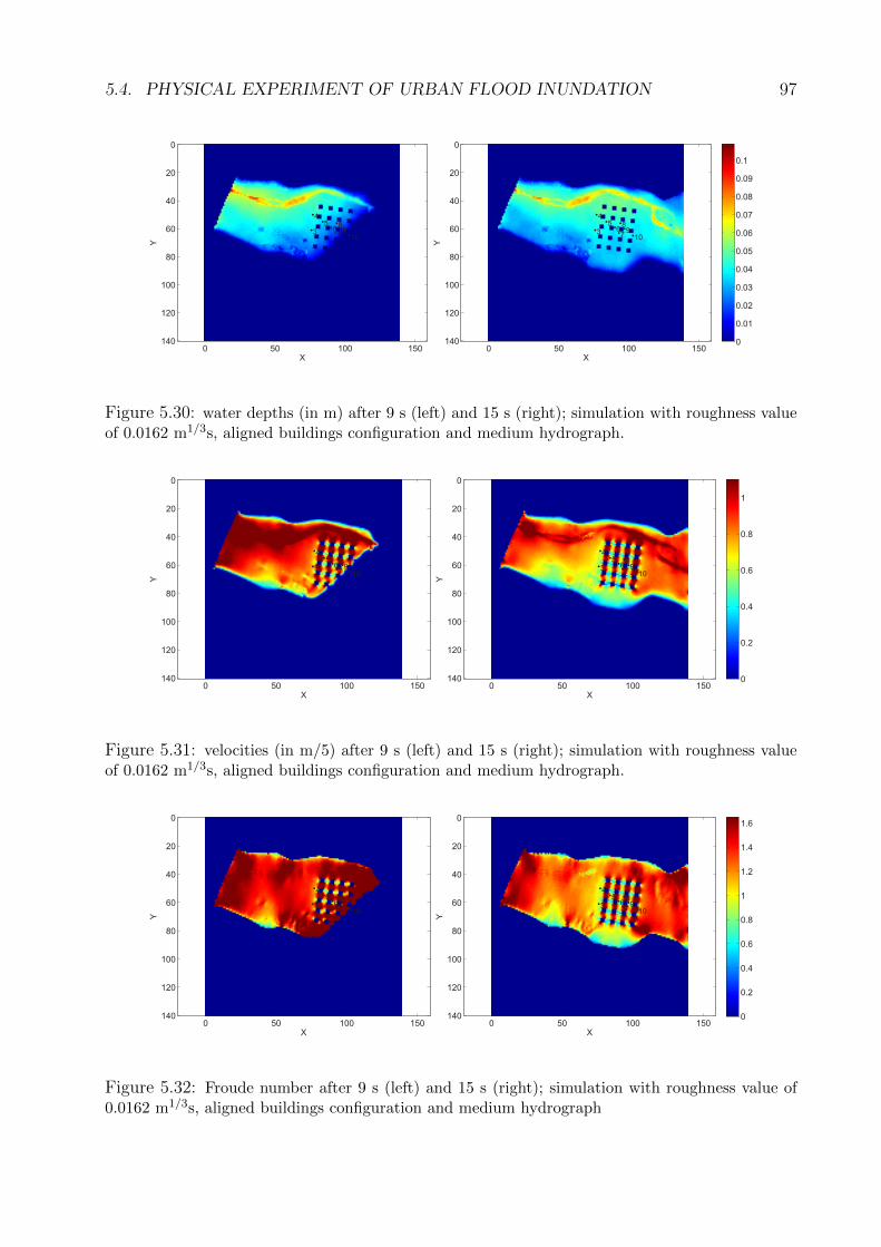
5.4. PHYSICAL EXPERIMENT OF URBAN FLOOD INUNDATION 97
3
4
56
7
89
10
X
Y
0 50 100 150
0
20
40
60
80
100
120
140 0
0.01
0.02
0.03
0.04
0.05
0.06
0.07
0.08
0.09
0.1
3
4
56
7
89
10
X
Y
0 50 100 150
0
20
40
60
80
100
120
140 0
0.01
0.02
0.03
0.04
0.05
0.06
0.07
0.08
0.09
0.1
Figure 5.30: water depths (in m) after 9 s (left) and 15 s (right); simulation with roughness valueof 0.0162 m1/3s, aligned buildings configuration and medium hydrograph.
3
4
56
7
89
10
X
Y
0 50 100 150
0
20
40
60
80
100
120
140 0
0.2
0.4
0.6
0.8
1
3
4
56
7
89
10
X
Y
0 50 100 150
0
20
40
60
80
100
120
140 0
0.2
0.4
0.6
0.8
1
Figure 5.31: velocities (in m/5) after 9 s (left) and 15 s (right); simulation with roughness valueof 0.0162 m1/3s, aligned buildings configuration and medium hydrograph.
3
4
56
7
89
10
X
Y
0 50 100 150
0
20
40
60
80
100
120
140 0
0.2
0.4
0.6
0.8
1
1.2
1.4
1.6
3
4
56
7
89
10
X
Y
0 50 100 150
0
20
40
60
80
100
120
140 0
0.2
0.4
0.6
0.8
1
1.2
1.4
1.6
Figure 5.32: Froude number after 9 s (left) and 15 s (right); simulation with roughness value of0.0162 m1/3s, aligned buildings configuration and medium hydrograph
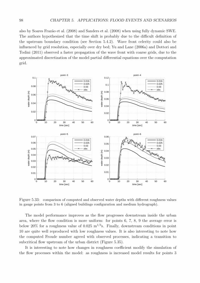
98 CHAPTER 5. APPLICATIONS: FLOOD EVENTS AND SCENARIOS
also by Soares Frazao et al. (2008) and Sanders et al. (2008) when using fully dynamic SWE.
The authors hypothesized that the time shift is probably due to the difficult definition of
the upstream boundary condition (see Section 5.4.2). Wave front celerity could also be
influenced by grid resolution, especially over dry bed; Yu and Lane (2006a) and Dottori and
Todini (2011) observed a faster propagation of the wave front with coarse grids, due to the
approximated discretization of the model partial differential equations over the computation
grid.
0 10 20 30 40 50 600
0.02
0.04
0.06
0.08
0.1
wat
er d
epth
(m
)
time [sec]
point−3
0.0160.0250.03obs
0 10 20 30 40 50 600
0.02
0.04
0.06
0.08
0.1
0.12
wat
er d
epth
(m
)
time [sec]
point−4
0.0160.0250.03obs
0 10 20 30 40 50 600
0.01
0.02
0.03
0.04
0.05
0.06
0.07
wat
er d
epth
(m
)
time [sec]
point−5
0.0160.0250.03obs
0 10 20 30 40 50 600
0.01
0.02
0.03
0.04
0.05
0.06
wat
er d
epth
(m
)
time [sec]
point−6
0.0160.0250.03obs
Figure 5.33: comparison of computed and observed water depths with different roughness valuesin gauge points from 3 to 6 (aligned buildings configuration and medium hydrograph).
The model performance improves as the flow progresses downstream inside the urban
area, where the flow condition is more uniform: for points 6, 7, 8, 9 the average error is
below 20% for a roughness value of 0.025 m1/3s. Finally, downstream conditions in point
10 are quite well reproduced with low roughness values. It is also interesting to note how
the computed Froude number agreed with observed processes, indicating a transition to
subcritical flow upstream of the urban district (Figure 5.35).
It is interesting to note how changes in roughness coefficient modify the simulation of
the flow processes within the model: as roughness is increased model results for points 3
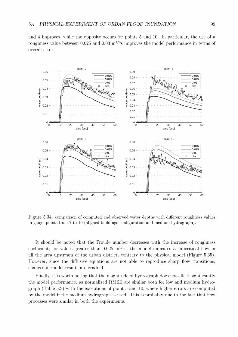
5.4. PHYSICAL EXPERIMENT OF URBAN FLOOD INUNDATION 99
and 4 improves, while the opposite occurs for points 5 and 10. In particular, the use of a
roughness value between 0.025 and 0.03 m1/3s improves the model performance in terms of
overall error.
0 10 20 30 40 50 600
0.01
0.02
0.03
0.04
0.05
0.06
wat
er d
epth
(m
)
time [sec]
point−7
0.0160.0250.03obs
0 10 20 30 40 50 600
0.01
0.02
0.03
0.04
0.05
0.06
0.07
0.08
0.09
wat
er d
epth
(m
)time [sec]
point−8
0.0160.0250.03obs
0 10 20 30 40 50 600
0.01
0.02
0.03
0.04
0.05
0.06
wat
er d
epth
(m
)
time [sec]
point−9
0.0160.0250.03obs
0 10 20 30 40 50 600
0.01
0.02
0.03
0.04
0.05
0.06
wat
er d
epth
(m
)
time [sec]
point−10
0.0160.0250.03obs
Figure 5.34: comparison of computed and observed water depths with different roughness valuesin gauge points from 7 to 10 (aligned buildings configuration and medium hydrograph).
It should be noted that the Froude number decreases with the increase of roughness
coefficient; for values greater than 0.025 m1/3s, the model indicates a subcritical flow in
all the area upstream of the urban district, contrary to the physical model (Figure 5.35).
However, since the diffusive equations are not able to reproduce sharp flow transitions,
changes in model results are gradual.
Finally, it is worth noting that the magnitude of hydrograph does not affect significantly
the model performance, as normalized RMSE are similar both for low and medium hydro-
graph (Table 5.3) with the exceptions of point 5 and 10, where higher errors are computed
by the model if the medium hydrograph is used. This is probably due to the fact that flow
processes were similar in both the experiments.
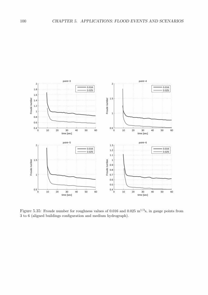
100 CHAPTER 5. APPLICATIONS: FLOOD EVENTS AND SCENARIOS
0 10 20 30 40 50 600.4
0.6
0.8
1
1.2
1.4
1.6
1.8
2
Fro
ude
num
ber
time [sec]
point−3
0.0160.025
0 10 20 30 40 50 600.5
1
1.5
2
Fro
ude
num
ber
time [sec]
point−4
0.0160.025
0 10 20 30 40 50 600.5
1
1.5
2
Fro
ude
num
ber
time [sec]
point−5
0.0160.025
0 10 20 30 40 50 600.4
0.5
0.6
0.7
0.8
0.9
1
1.1
1.2
1.3
Fro
ude
num
ber
time [sec]
point−6
0.0160.025
Figure 5.35: Froude number for roughness values of 0.016 and 0.025 m1/3s, in gauge points from3 to 6 (aligned buildings configuration and medium hydrograph).
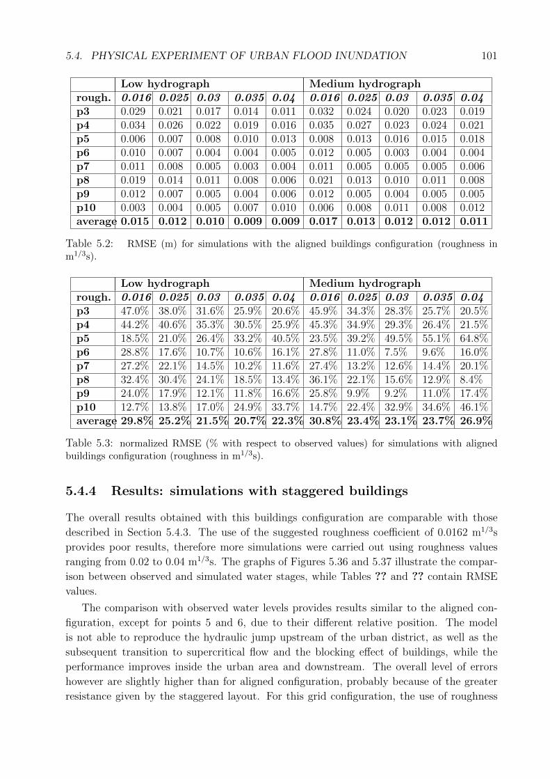
5.4. PHYSICAL EXPERIMENT OF URBAN FLOOD INUNDATION 101
Low hydrograph Medium hydrographrough. 0.016 0.025 0.03 0.035 0.04 0.016 0.025 0.03 0.035 0.04p3 0.029 0.021 0.017 0.014 0.011 0.032 0.024 0.020 0.023 0.019p4 0.034 0.026 0.022 0.019 0.016 0.035 0.027 0.023 0.024 0.021p5 0.006 0.007 0.008 0.010 0.013 0.008 0.013 0.016 0.015 0.018p6 0.010 0.007 0.004 0.004 0.005 0.012 0.005 0.003 0.004 0.004p7 0.011 0.008 0.005 0.003 0.004 0.011 0.005 0.005 0.005 0.006p8 0.019 0.014 0.011 0.008 0.006 0.021 0.013 0.010 0.011 0.008p9 0.012 0.007 0.005 0.004 0.006 0.012 0.005 0.004 0.005 0.005p10 0.003 0.004 0.005 0.007 0.010 0.006 0.008 0.011 0.008 0.012average 0.015 0.012 0.010 0.009 0.009 0.017 0.013 0.012 0.012 0.011
Table 5.2: RMSE (m) for simulations with the aligned buildings configuration (roughness inm1/3s).
Low hydrograph Medium hydrographrough. 0.016 0.025 0.03 0.035 0.04 0.016 0.025 0.03 0.035 0.04p3 47.0% 38.0% 31.6% 25.9% 20.6% 45.9% 34.3% 28.3% 25.7% 20.5%p4 44.2% 40.6% 35.3% 30.5% 25.9% 45.3% 34.9% 29.3% 26.4% 21.5%p5 18.5% 21.0% 26.4% 33.2% 40.5% 23.5% 39.2% 49.5% 55.1% 64.8%p6 28.8% 17.6% 10.7% 10.6% 16.1% 27.8% 11.0% 7.5% 9.6% 16.0%p7 27.2% 22.1% 14.5% 10.2% 11.6% 27.4% 13.2% 12.6% 14.4% 20.1%p8 32.4% 30.4% 24.1% 18.5% 13.4% 36.1% 22.1% 15.6% 12.9% 8.4%p9 24.0% 17.9% 12.1% 11.8% 16.6% 25.8% 9.9% 9.2% 11.0% 17.4%p10 12.7% 13.8% 17.0% 24.9% 33.7% 14.7% 22.4% 32.9% 34.6% 46.1%average 29.8% 25.2% 21.5% 20.7% 22.3% 30.8% 23.4% 23.1% 23.7% 26.9%
Table 5.3: normalized RMSE (% with respect to observed values) for simulations with alignedbuildings configuration (roughness in m1/3s).
5.4.4 Results: simulations with staggered buildings
The overall results obtained with this buildings configuration are comparable with those
described in Section 5.4.3. The use of the suggested roughness coefficient of 0.0162 m1/3s
provides poor results, therefore more simulations were carried out using roughness values
ranging from 0.02 to 0.04 m1/3s. The graphs of Figures 5.36 and 5.37 illustrate the compar-
ison between observed and simulated water stages, while Tables ?? and ?? contain RMSE
values.
The comparison with observed water levels provides results similar to the aligned con-
figuration, except for points 5 and 6, due to their different relative position. The model
is not able to reproduce the hydraulic jump upstream of the urban district, as well as the
subsequent transition to supercritical flow and the blocking effect of buildings, while the
performance improves inside the urban area and downstream. The overall level of errors
however are slightly higher than for aligned configuration, probably because of the greater
resistance given by the staggered layout. For this grid configuration, the use of roughness
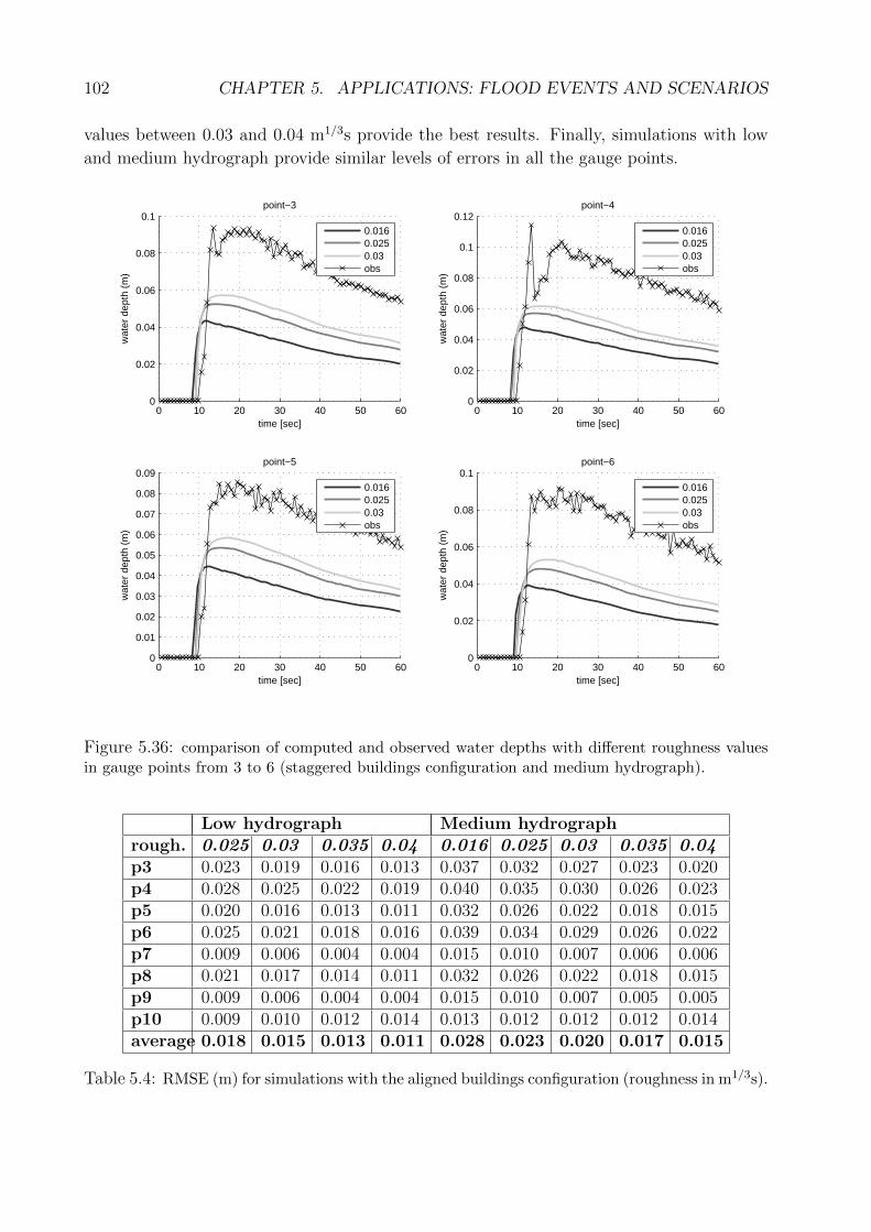
102 CHAPTER 5. APPLICATIONS: FLOOD EVENTS AND SCENARIOS
values between 0.03 and 0.04 m1/3s provide the best results. Finally, simulations with low
and medium hydrograph provide similar levels of errors in all the gauge points.
0 10 20 30 40 50 600
0.02
0.04
0.06
0.08
0.1
wat
er d
epth
(m
)
time [sec]
point−3
0.0160.0250.03obs
0 10 20 30 40 50 600
0.02
0.04
0.06
0.08
0.1
0.12
wat
er d
epth
(m
)
time [sec]
point−4
0.0160.0250.03obs
0 10 20 30 40 50 600
0.01
0.02
0.03
0.04
0.05
0.06
0.07
0.08
0.09
wat
er d
epth
(m
)
time [sec]
point−5
0.0160.0250.03obs
0 10 20 30 40 50 600
0.02
0.04
0.06
0.08
0.1
wat
er d
epth
(m
)
time [sec]
point−6
0.0160.0250.03obs
Figure 5.36: comparison of computed and observed water depths with different roughness valuesin gauge points from 3 to 6 (staggered buildings configuration and medium hydrograph).
Low hydrograph Medium hydrographrough. 0.025 0.03 0.035 0.04 0.016 0.025 0.03 0.035 0.04p3 0.023 0.019 0.016 0.013 0.037 0.032 0.027 0.023 0.020p4 0.028 0.025 0.022 0.019 0.040 0.035 0.030 0.026 0.023p5 0.020 0.016 0.013 0.011 0.032 0.026 0.022 0.018 0.015p6 0.025 0.021 0.018 0.016 0.039 0.034 0.029 0.026 0.022p7 0.009 0.006 0.004 0.004 0.015 0.010 0.007 0.006 0.006p8 0.021 0.017 0.014 0.011 0.032 0.026 0.022 0.018 0.015p9 0.009 0.006 0.004 0.004 0.015 0.010 0.007 0.005 0.005p10 0.009 0.010 0.012 0.014 0.013 0.012 0.012 0.012 0.014average 0.018 0.015 0.013 0.011 0.028 0.023 0.020 0.017 0.015
Table 5.4: RMSE (m) for simulations with the aligned buildings configuration (roughness in m1/3s).
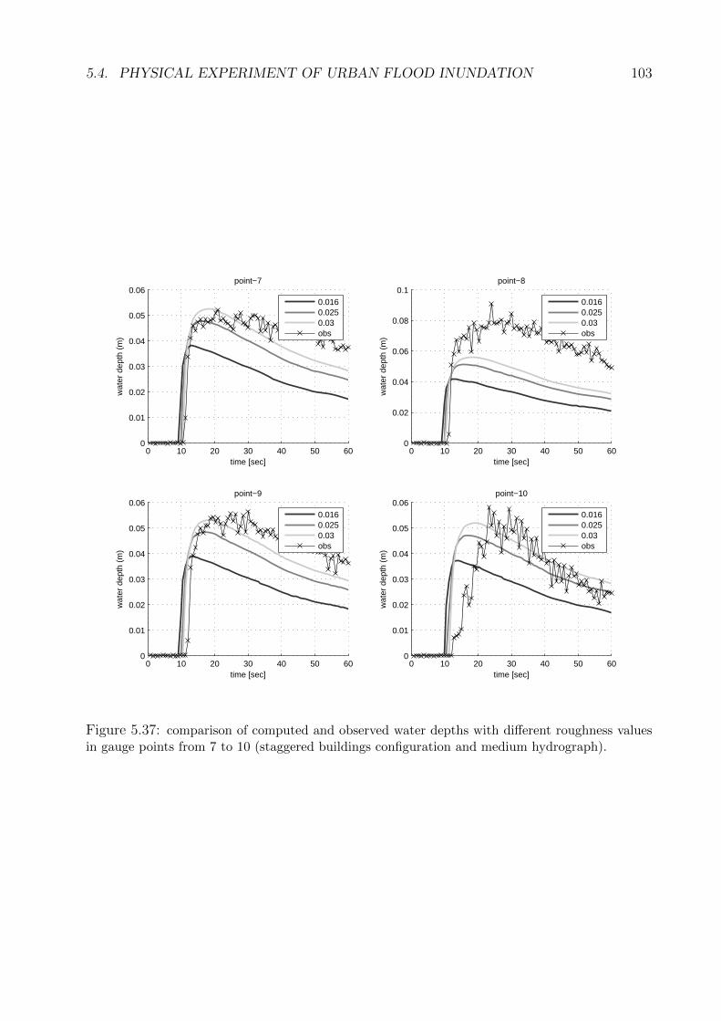
5.4. PHYSICAL EXPERIMENT OF URBAN FLOOD INUNDATION 103
0 10 20 30 40 50 600
0.01
0.02
0.03
0.04
0.05
0.06
wat
er d
epth
(m
)
time [sec]
point−7
0.0160.0250.03obs
0 10 20 30 40 50 600
0.02
0.04
0.06
0.08
0.1
wat
er d
epth
(m
)
time [sec]
point−8
0.0160.0250.03obs
0 10 20 30 40 50 600
0.01
0.02
0.03
0.04
0.05
0.06
wat
er d
epth
(m
)
time [sec]
point−9
0.0160.0250.03obs
0 10 20 30 40 50 600
0.01
0.02
0.03
0.04
0.05
0.06
wat
er d
epth
(m
)
time [sec]
point−10
0.0160.0250.03obs
Figure 5.37: comparison of computed and observed water depths with different roughness valuesin gauge points from 7 to 10 (staggered buildings configuration and medium hydrograph).
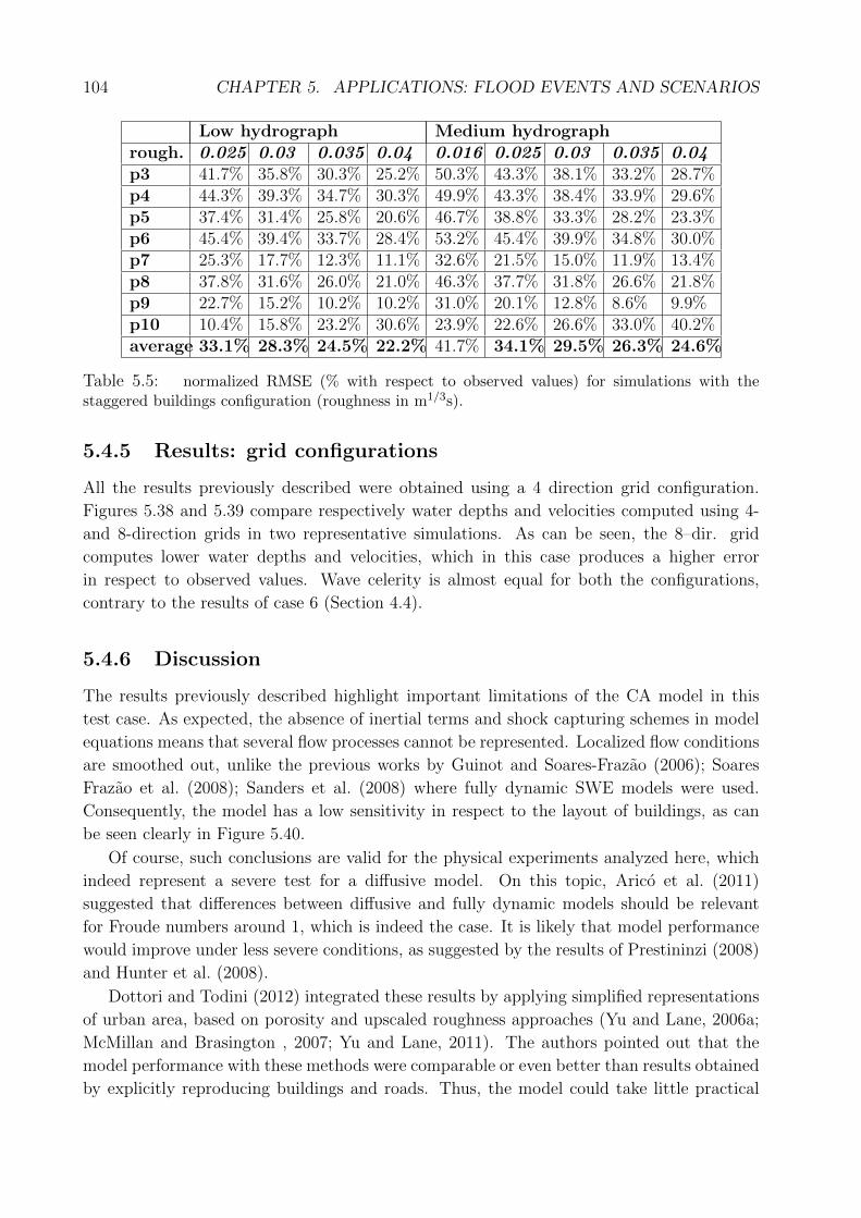
104 CHAPTER 5. APPLICATIONS: FLOOD EVENTS AND SCENARIOS
Low hydrograph Medium hydrographrough. 0.025 0.03 0.035 0.04 0.016 0.025 0.03 0.035 0.04p3 41.7% 35.8% 30.3% 25.2% 50.3% 43.3% 38.1% 33.2% 28.7%p4 44.3% 39.3% 34.7% 30.3% 49.9% 43.3% 38.4% 33.9% 29.6%p5 37.4% 31.4% 25.8% 20.6% 46.7% 38.8% 33.3% 28.2% 23.3%p6 45.4% 39.4% 33.7% 28.4% 53.2% 45.4% 39.9% 34.8% 30.0%p7 25.3% 17.7% 12.3% 11.1% 32.6% 21.5% 15.0% 11.9% 13.4%p8 37.8% 31.6% 26.0% 21.0% 46.3% 37.7% 31.8% 26.6% 21.8%p9 22.7% 15.2% 10.2% 10.2% 31.0% 20.1% 12.8% 8.6% 9.9%p10 10.4% 15.8% 23.2% 30.6% 23.9% 22.6% 26.6% 33.0% 40.2%average 33.1% 28.3% 24.5% 22.2% 41.7% 34.1% 29.5% 26.3% 24.6%
Table 5.5: normalized RMSE (% with respect to observed values) for simulations with thestaggered buildings configuration (roughness in m1/3s).
5.4.5 Results: grid configurations
All the results previously described were obtained using a 4 direction grid configuration.
Figures 5.38 and 5.39 compare respectively water depths and velocities computed using 4-
and 8-direction grids in two representative simulations. As can be seen, the 8–dir. grid
computes lower water depths and velocities, which in this case produces a higher error
in respect to observed values. Wave celerity is almost equal for both the configurations,
contrary to the results of case 6 (Section 4.4).
5.4.6 Discussion
The results previously described highlight important limitations of the CA model in this
test case. As expected, the absence of inertial terms and shock capturing schemes in model
equations means that several flow processes cannot be represented. Localized flow conditions
are smoothed out, unlike the previous works by Guinot and Soares-Frazao (2006); Soares
Frazao et al. (2008); Sanders et al. (2008) where fully dynamic SWE models were used.
Consequently, the model has a low sensitivity in respect to the layout of buildings, as can
be seen clearly in Figure 5.40.
Of course, such conclusions are valid for the physical experiments analyzed here, which
indeed represent a severe test for a diffusive model. On this topic, Arico et al. (2011)
suggested that differences between diffusive and fully dynamic models should be relevant
for Froude numbers around 1, which is indeed the case. It is likely that model performance
would improve under less severe conditions, as suggested by the results of Prestininzi (2008)
and Hunter et al. (2008).
Dottori and Todini (2012) integrated these results by applying simplified representations
of urban area, based on porosity and upscaled roughness approaches (Yu and Lane, 2006a;
McMillan and Brasington , 2007; Yu and Lane, 2011). The authors pointed out that the
model performance with these methods were comparable or even better than results obtained
by explicitly reproducing buildings and roads. Thus, the model could take little practical
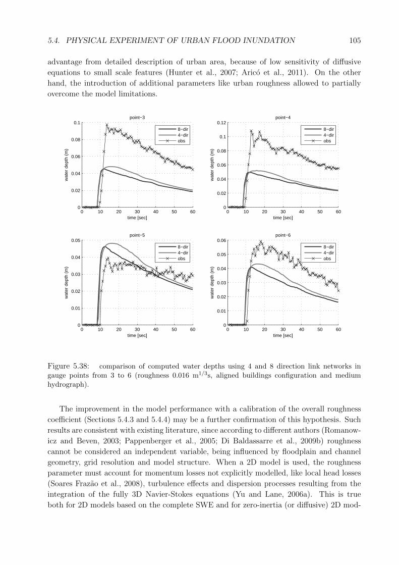
5.4. PHYSICAL EXPERIMENT OF URBAN FLOOD INUNDATION 105
advantage from detailed description of urban area, because of low sensitivity of diffusive
equations to small scale features (Hunter et al., 2007; Arico et al., 2011). On the other
hand, the introduction of additional parameters like urban roughness allowed to partially
overcome the model limitations.
0 10 20 30 40 50 600
0.02
0.04
0.06
0.08
0.1
wat
er d
epth
(m
)
time [sec]
point−3
8−dir4−dirobs
0 10 20 30 40 50 600
0.02
0.04
0.06
0.08
0.1
0.12
wat
er d
epth
(m
)time [sec]
point−4
8−dir4−dirobs
0 10 20 30 40 50 600
0.01
0.02
0.03
0.04
0.05
wat
er d
epth
(m
)
time [sec]
point−5
8−dir4−dirobs
0 10 20 30 40 50 600
0.01
0.02
0.03
0.04
0.05
0.06
wat
er d
epth
(m
)
time [sec]
point−6
8−dir4−dirobs
Figure 5.38: comparison of computed water depths using 4 and 8 direction link networks ingauge points from 3 to 6 (roughness 0.016 m1/3s, aligned buildings configuration and mediumhydrograph).
The improvement in the model performance with a calibration of the overall roughness
coefficient (Sections 5.4.3 and 5.4.4) may be a further confirmation of this hypothesis. Such
results are consistent with existing literature, since according to different authors (Romanow-
icz and Beven, 2003; Pappenberger et al., 2005; Di Baldassarre et al., 2009b) roughness
cannot be considered an independent variable, being influenced by floodplain and channel
geometry, grid resolution and model structure. When a 2D model is used, the roughness
parameter must account for momentum losses not explicitly modelled, like local head losses
(Soares Frazao et al., 2008), turbulence effects and dispersion processes resulting from the
integration of the fully 3D Navier-Stokes equations (Yu and Lane, 2006a). This is true
both for 2D models based on the complete SWE and for zero-inertia (or diffusive) 2D mod-
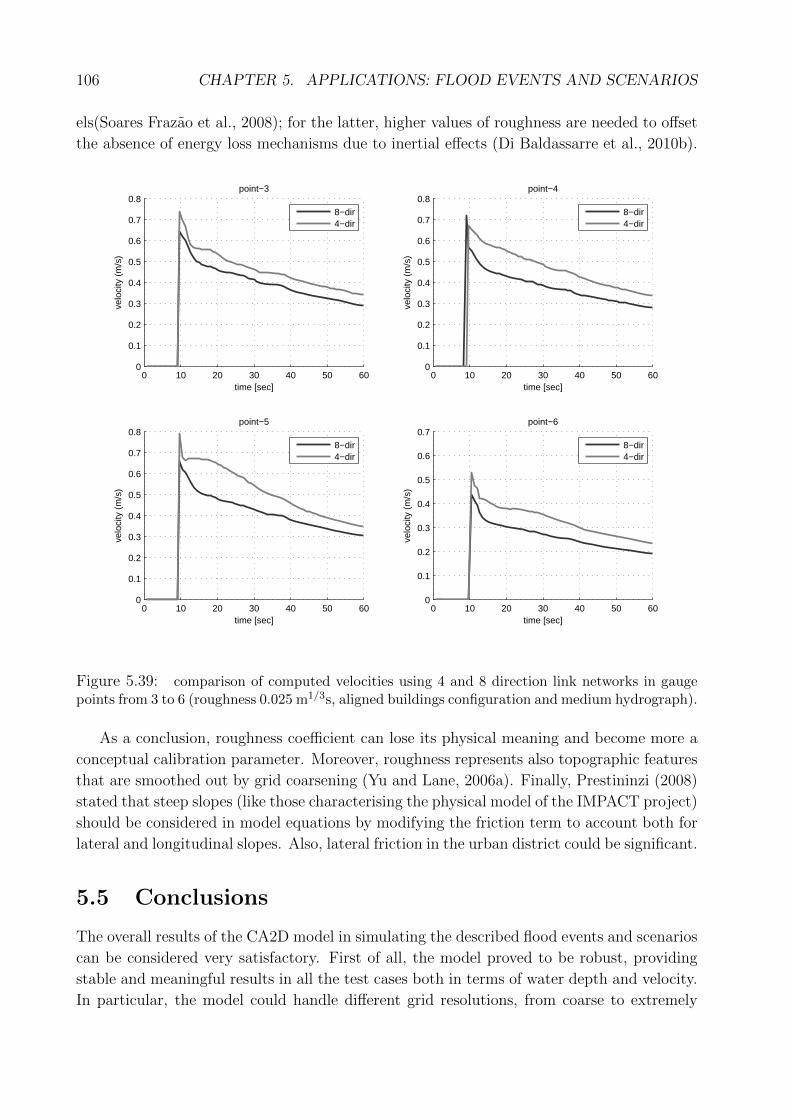
106 CHAPTER 5. APPLICATIONS: FLOOD EVENTS AND SCENARIOS
els(Soares Frazao et al., 2008); for the latter, higher values of roughness are needed to offset
the absence of energy loss mechanisms due to inertial effects (Di Baldassarre et al., 2010b).
0 10 20 30 40 50 600
0.1
0.2
0.3
0.4
0.5
0.6
0.7
0.8
velo
city
(m
/s)
time [sec]
point−3
8−dir4−dir
0 10 20 30 40 50 600
0.1
0.2
0.3
0.4
0.5
0.6
0.7
0.8
velo
city
(m
/s)
time [sec]
point−4
8−dir4−dir
0 10 20 30 40 50 600
0.1
0.2
0.3
0.4
0.5
0.6
0.7
0.8
velo
city
(m
/s)
time [sec]
point−5
8−dir4−dir
0 10 20 30 40 50 600
0.1
0.2
0.3
0.4
0.5
0.6
0.7
velo
city
(m
/s)
time [sec]
point−6
8−dir4−dir
Figure 5.39: comparison of computed velocities using 4 and 8 direction link networks in gaugepoints from 3 to 6 (roughness 0.025 m1/3s, aligned buildings configuration and medium hydrograph).
As a conclusion, roughness coefficient can lose its physical meaning and become more a
conceptual calibration parameter. Moreover, roughness represents also topographic features
that are smoothed out by grid coarsening (Yu and Lane, 2006a). Finally, Prestininzi (2008)
stated that steep slopes (like those characterising the physical model of the IMPACT project)
should be considered in model equations by modifying the friction term to account both for
lateral and longitudinal slopes. Also, lateral friction in the urban district could be significant.
5.5 Conclusions
The overall results of the CA2D model in simulating the described flood events and scenarios
can be considered very satisfactory. First of all, the model proved to be robust, providing
stable and meaningful results in all the test cases both in terms of water depth and velocity.
In particular, the model could handle different grid resolutions, from coarse to extremely

5.5. CONCLUSIONS 107
fine (up to 5cm in the urban flood scenario described in Section 5.4); mixed 1D and 2D flow
processes both on mild and steep slopes; test sites with complex topography, including large
obstacles like embankments and levees, and localized obstacles like buildings.
0 10 20 30 40 50 600
0.01
0.02
0.03
0.04
0.05
0.06
wat
er d
epth
(m
)
time [sec]
point−7
sim aligsim stagobs alig
0 10 20 30 40 50 600
0.01
0.02
0.03
0.04
0.05
0.06
0.07
0.08
0.09
wat
er d
epth
(m
)time [sec]
point−8
sim aligsim stagobs alig
0 10 20 30 40 50 600
0.01
0.02
0.03
0.04
0.05
0.06
wat
er d
epth
(m
)
time [sec]
point−9
sim aligsim stagobs alig
0 10 20 30 40 50 600
0.01
0.02
0.03
0.04
0.05
wat
er d
epth
(m
)
time [sec]
point−10
sim aligsim stagobs alig
Figure 5.40: Comparison of computed water depths for aligned and staggered layouts, and obser-vations with aligned layout in gauge points from 7 to 10 (experiment with medium hydrograph).
The model reproduced well flood events characterized by slow 1D and 2D flow processes,
like those occurred in rivers Reno and Po (Sections 5.1, 5.2). Good results were obtained
also in the application to the River Ubaye (Section 5.3), characterized by high resolution
grids and steep slopes. In all these applications,the accuracy of model results was adequate
to large scale analysis, and compatible with the uncertainty of available data for model
construction and validation. Sensitivity analyses were carried out to investigate the effect of
roughness calibration; the resulting values were physically meaningful and comparable with
usual values for 2D hydraulic models.
The application to urban flood scenario experiments gave less satisfactory results (Section
5.4). The model was able to simulate the overall flow processes, but it could not capture
the details of the complex processes produced by the interaction of buildings with the flow,
such as hydraulic jumps and wake effects. However such results were expected, due to the

108 CHAPTER 5. APPLICATIONS: FLOOD EVENTS AND SCENARIOS
severity of the test case and the approximations in model equations. Under less severe
flow conditions and when localized flow conditions are not of interest, the performances of
diffusive 2D models are likely to be acceptable.
Chapter 6
Conclusions
The main objective of the described research work was to develop reliable models for large
scale analysis of flood inundation events and scenarios. Two different models, CA2D and
IFD-GGA, were developed, adopting a partially integrated approach and testing different
configurations. Overall results highlighted relevant differences between the performance of
the two models.
The performances of the CA2D model were very satisfactory. The model proved to be
fast and robust, providing stable and consistent results in all the test cases, both in terms
of water level and velocity. The model could reproduce mixed 1D and 2D flow processes
and it could handle complex topographic features, including steep slopes, large obstacles like
embankments and levees, and localized obstacles like buildings. Finally, the simple model
structure and the use of methods to increase model stability enabled reduced computation
times, which were faster or comparable to established 2D hydraulic models.
The model reproduced well test cases characterized by slow 1D and 2D flow processes. In
these applications, the accuracy of model results was adequate to large scale analysis, and the
magnitude of observed errors was below the typical uncertainty of data and observations in
actual flood events, e.g. topography and inundation extent maps. The model performance
was less satisfactory in test cases characterized by complex flow processes, such as flow
transitions and interaction with obstacles. In these cases relevant local errors were observed,
due to the diffusive form of the governing equations, which can not capture inertial effects
and shock waves. However, local conditions did not compromise the ability of the model to
correctly simulate overall flow processes, and in most cases the error was limited.
In conclusion, the results suggest that the CA model can be a valuable tool for the
simulation of a wide range of flood event types.
On the contrary, the results of the IFD-GGA model in the considered numerical cases
were not satisfactory. Except for simple 1D and 2D numerical cases, the different model
versions showed serious problems and the poor performance of model algorithms prevented
further applications. Therefore the work on the IFD-GGA model was interrupted and its
development is now being reconsidered. A possible solution could be the use of the fully
dynamic SWE as governing equations, while maintaining the existing model structure to
preserve the integration with CA2D. This would enable a coupled application of the two
109
110 CHAPTER 6. CONCLUSIONS
models: for instance, IFD-GGA could be applied where localized complex flow conditions
are expected, while using CA2D in the rest of the study area. However, model development
in this sense has not been undertaken yet.
6.1 Further developments of the model codes
So far, the CA2D model has been primarily used to reproduce flow routing and associated
lowland flood events. However, numerical and practical applications (e.g. case 2, Section
4.2) demonstrated that the model is able to reproduce overland and concentrated flow and
manage wetting and drying effects over wide areas (from hillslope up to small basin scale).
Therefore the model could be used to simulate the surface runoff produced by intense rainfall
events, including the formation of flash floodss and the analysis of related risk. However,
the CA2D model should undergo adequate calibration tests before being applied in similar
studies.
Within this framework, the model structure could be expanded to include more hydro-
logical processes. For instance, the simulation of infiltration could be improved by imple-
menting more complex methods like Horton and Green-Ampt. Accordingly, subsurface flow
and soil moisture can be introduced without substantial modifications of model structure,
improving the capacity of CA2D to reproduce event-based hydrological processes on small
basins or hillslopes. Finally, soil erosion and sediment transport associated to overland flow
could also be implemented within the model.
Besides these additions, further research would be needed to exploit the flexible struc-
ture of the model. The results described in Chapters 4 and 5 suggest that the diffusive
and inertial formulations could be proficiently integrated and used alternatively, depending
on flow conditions. However, more research to establish empirical or numerical criteria is
needed. Similar criteria should be investigated to allow the integrated use of 8 directions
and 4 directions link networks. Finally, additional functions are currently being implemen-
ted and tested in the model codes, to expand the basic versions described in Chapter 3.
For instance, subgrid parameterizations can be used to characterize the geometry of grid
elements (cells and connections), to simulate more accurately 1D open channel flows or to
represent microtopography over coarse grids (Yu and Lane, 2006a; McMillan and Brasington
, 2007; Yu and Lane, 2011; Dottori and Todini, 2012).
6.2 Future applications of the models
As mentioned in Section 3.5, the CA2D model is currently being integrated in the information
system of the Civil Protection Agency. The first objective is to use CA2D to analyze flood
scenarios caused by dyke breach and dyke overtopping along the main rivers of the Emilia-
Romagna district. A further objective should be to integrate CA2D in the existing flood
modelling system composed by meteorological, hydrological and 1D hydraulic models. This
would allow more accurate flood risk analysis, including real-time forecasting of flood events.
6.2. FUTURE APPLICATIONS OF THE MODELS 111
To this end, the parallelisation of the model code on distributed multiprocessor machines
and GPU cards has also been planned (Section 3.5).
Besides these specific applications, diffusive reduced complexity models like CA2D could
be used to perform flood analysis at very large scale (even continental scale), exploiting the
new remote sensing and freely available data sources that should be available in a few years
(Di Baldassarre and Ulhenbrook, 2012). This would allow to produce reliable flood maps
in countries where either scarce or no information of flood risk is available, thus providing
a considerable contribute both to research works and flood risk management in developing
countries. Actually, the CA2D model has already been used in a similar framework to
develop probabilistic flood mapping of a large part of Italy, for insurance porpuses. Existing
databases of past flood events and freely available remote sensing data were used for model
construction and validation, with good results.
Finally, the developed models could be released as free, open source softwares. Nowadays
a number of established flood inundation models are available as free softwares and can
be downloaded from the website of respective developing institutions or companies (e.g.
LISFLOOD-FP (www.bris.ac.uk/geography/research/hydrology/models/lisflood), and the
CCHE2D model (www.ncche.olemiss.edu). On the other hand other model codes are
available as open source software, for instance TELEMAC-2D (www.opentelemac.org) and
XBEACH (http : //oss.deltares.nl/web/xbeach). The availability of reliable free and open
source flood inundation models can extremely useful especially (but not only) in developing
countries, to increase the know-how of technicians and practitioners and to enable adequate
flood risk analyses. Moreover, open source models are particulary suited for didactical and
research purposes, allowing to learn how a model code can be developed, modified and
expanded.
Indeed, this would probably be an excellent way to spread the results of the research
work described in this thesis. Hopefully, this thesis will also be a small contribute to improve
current and future flood risk management and mitigation strategies.

112 CHAPTER 6. CONCLUSIONS
Bibliography
Alcrudo, F., 2004. Mathematical Modelling Techniques for Flood Propagation in Urban
Areas. IMPACT Project technical report (www.impact− project.net).
Anselmo, V., Galeati, G., Palmieri, S., Rossi, U., Todini, E., 1996. Flood risk assessment
using an integrated hydrological-hydraulic modelling approach: a case study, J. Hydrol.
175, 533-554.
Arico, C.,Sinagra, M., Begnudelli, L., Tucciarelli, T., 2011. MAST-2D diffusive model for
flood prediction on domains with triangular Delaunay unstructured meshes. Adv. Water
Res. 34,1427-1449.
Aronica, G., Hankinb B., Beven, K., 1998.Uncertainty and equifinality in calibrating distrib-
uted roughness coefficients in a flood propagation model with limited data. Adv. Water
Res. 22 (4), 349–365.
Avolio, M.V., Crisci, G.M., Di Gregorio, S., Rongo, R., William Spataro, W., D’Ambrosio,
D., 2006. Pyroclastic flows modelling using cellular automata. Computers & Geosciences
32, 897-911.
Bagarello, V., Ferro, V., 2006. Erosion and soil conservation (in Italian), McGraw-Hill,
Milano.
Bateman, A., Medina, V., Velasco, V., 2010. Soil infiltration effect in flat areas floods simu-
lation. In: J. Carrera (Ed.) XVIII International Conference on Water Resources CMWR
2010, Barcelona (Spain).
Bates, P.D., de Roo, A.P.J., 2000. A simple Raster-Based Model For Flood Inundation
Simulation. J. Hydrol. 236, 54-77.
Bates, P.D., 2004. Remote sensing and flood inundation modelling. Hydrol. Proces. 18, 2593–
2597.
Bates, P.D., Wilson, M.D., Horritt, M.S., Mason, D.C., Holden, N., Currie, A., 2006. Reach
scale floodplain inundation dynamics observed using airborne synthetic aperture radar
imagery: Data analysis and modelling. J. Hydrol. 328, 306-318
113
114 BIBLIOGRAPHY
Bates, P.D., Horritt, M.S., Fewtrell, T.J., 2010. A simple inertial formulation of the shallow
water equations for efficient two-dimensional flood inundation modelling. J. Hydrol. 387,
33-45.
Bradbrook, K.F., Lane, S.N., Waller, S.G., Bates, P.D., 2004. Two dimensional diffusion
wave modelling of flood inundation using a simplified channel representation. International
Journal of River Basin Management 3, 1–13.
Casulli, V., 1990. Semi-implicit Finite Difference Methods for the Two- Dimensional Shallow
Water Equations. Journal of Computational Physics, 86, 56-74.
Casulli, V., Stelling, G.S., 2010. Semi-implicit subgrid modelling of three-dimensional free
surface flows, Int. Jour. for Numer. Meth. Fluids, DOI: 10.1002/fld2361.
Castellarin, A., Domeneghetti, A., and Brath, A. (2011). Identifying robust large-scale flood
risk miti gation strategies: a quasi-2D hydraulic model as a tool for the Po river, Phys.
Chem. Earth, 36, 299-308.
Chopard, B., Masselot, A., 1999. Cellular automata and lattice Boltzmann methods: a
new approach to computational fluid dynamics and particle transport. Future Generation
Computer Systems 16, 249-257.
Chow, V.T., 1959. Open-Channel Hydraulics. MCGraw-Hill, New York.
Cockburn, B., Shu, C.W., 2001. RungeKutta Discontinuous Galerkin Methods for
Convection-Dominated Problems. Journal of Scientific Computing 16-3, 173-261.
Commission of the European Community, 1996. AFORISM, a Comprehensive Forecasting
System for Flood risk Mitigation and Control, Final Report.
Commission of the European Community, 2007. Directive 2007/60/EC on the assessment
and management of flood risks. Official Journal of the European Union.
Cremonini, 1994. Autopsy of a fluvial breach (in Italian), Il Carrobbio 20, 339-362, 1994.
Crossley, A.J., Wright, N.G., Chris D. Whitlow, C.D., 2003. Local Time Stepping for Mod-
eling Open Channel Flows. J. Hydraul. Eng. 129(6), 455-462.
Cunge, J.A., 2003. Of data and models. J. Hydroinf. 5(2), 75-98.
D’Ambrosio, D., Di Gregorio, S., Iovine, G., 2003. Simulating debris flows through a
hexagonal cellular automata model: SCIDDICA S3-hex. Natural Hazards and Earth Sys-
tem Sciences 3, 545–559.
Danish Hydraulic Institute (DHI) Water and Environment, 2000. Mike21, Danish Hydraulic
Institute, Horsholm, Denmark.
BIBLIOGRAPHY 115
Di Baldassarre, G., Castellarin, A., Brath, A., 2009a. Analysis on the effects of levee height-
ening on flood propagation: some thoughts on the River Po. Hydrol. Sci. J. 54(6),1007–17.
Di Baldassarre, G., Schumann, G.J.-P., Bates, P.D., 2009b. Near real time satellite imagery
to support and verify timely flood modelling. Hydrol Process, 23, 799–803.
Di Baldassarre, G., Montanari, A., Lins, H., Koutsoyiannis, D., Brandimarte, L., Blschl, G.,
2010. Flood fatalities in Africa: From diagnosis to mitigation, Geophys. Res. Lett., 37,
L22402, doi:10.1029/2010GL045467.
Di Baldassarre, G., Schumann, G., Bates, P.D., Freer, J.E., Beven, K.J., 2010. Floodplain
mapping: a critical discussion of deterministic and probabilistic approaches. Hydrol. Sci.
J. 55(3), 364–376.
Di Baldassarre, G., and Ulhenbrook, S., 2012. Is the current flood of data enough? A treatise
on research needs for the improvement of flood modelling. Hydrol. Process. 26, 153–158.
Di Giammarco, P., Todini, E., Lamberti, P., 1996. A conservative finite elements approach
to overland flow: the control volume finite element formulation. J. Hydrol. 175 (1-4),
267–291.
Dottori, F., Todini, E., 2010a. A 2D flood inundation model based on an implicit parallel-
izable scheme. In: J. Carrera (Ed.), XVIII International Conference on Water Resources
CMWR 2010, Barcelona (Spain).
Dottori, F., Todini, E., 2010b. A 2D flood inundation model based on cellular atomata ap-
proach. In: J. Carrera (Ed.), XVIII International Conference on Water Resources CMWR
2010, Barcelona (Spain).
Dottori, F., Todini, E., 2011. Developments of a flood inundation model based on the cellular
atomata approach: testing different methods to improve model performance. Phys. Chem.
Earth 36 (2011) 266-280.
Dottori, F., Alfonso, L., Di Baldassarre, G., 2011. The value of urban flood mapping: ap-
plication to the case study of Barcelonnette (France). EGU 2011 Leonardo Conference,
Bratislava.
Dottori, F., Todini, E., 2012. Testing a simple 2D hydraulic model in an urban ood experi-
ment. Hydrol.l Proces. under review.
El Kadi Abderrezzak, K., Paquier, A., Mignot, E., 2009. Modelling flash flood propagation
in urban areas using a two-dimensional numerical model. Nat. Hazards 50, 433–460.
Emergency Events Database 2011. OFDA/CRED International Disaster Database, Uni-
versite Catholique de Louvain, Brussels, http : //www.cred.be/emdat.
116 BIBLIOGRAPHY
Ern, A., Piperno, S., Djadel, K., 2008. A well-balanced RungeKutta Discontinuous Galerkin
method for the Shallow-Water Equations with flooding and drying. Int. J. Numer. Meth.
Fluids. 58(1), 1–25.
U.S. Federal Emergency Management Agency. Numerical Models Meeting the Minimum
Requirements of the National Flood Insurance Program. 11-Aug-2010 12:08 UTC (cited
2012 Feb 24). Available from: http : //www.fema.gov/plan/prevent/fhm/en modl.shtm
Ferro, V., 2006. Management of river basins (in Italian), McGraw-Hill, Milano.
Fewtrell, T.J., Bates, P.D., Horritt, M.S., Trigg, M.A., 2007. The effect of temporal and
spatial coarsening on storage cell predictions of urban flood inundation., 32nd Congress
of the International Association for Hydraulic Engineering and Research, Venice, Italy, 1,
37-47, ISBN: 8889405066.
Fewtrell, T.J., Bates, P.D., Horritt, M.S., Hunter, N.M., 2008. Evaluating the effect of scale
in flood inundation modelling in urban environments. Hydrol. Proc. 22, 5107-5118
Fewtrell, T.J., Duncan, A., Sampson, C.C., Neal, J.C., Bates, P.D., 2011. Benchmarking
urban flood models of varying complexity and scale using high resolution terrestrial LiDAR
data. Phys. Chem. Earth 36 (2011).
FLO-2D Software Inc., 2007. FLO-2D Users Manual (2007).
Gallegos, H.A., Schubert, J.E., Sanders, B.F., 2009. Two-dimensional, high-resolution mod-
eling of urban dam-break flooding: a case study of Baldwin Hills, California. Adv. Water
Res. 32, 1323–1335.
Gotzinger J, Bardossy A. 2008. Generic error model for calibration and uncer-
tainty estimation of hydrological models. Water Resources Research W00B07:
DOI:10.1029/2007WR006691.
Guinot, V., Soares-Frazao, S., 2006. Flux and source term discretization in two-dimensional
shallow water models with porosity on unstructured grids. Int. J. Numer. Meth. Fluids
50, 309–345.
Guinot, V., Cappeleare, B., 2009. Sensitivity analysis of 2D steady-state shallow water flow.
Application to free surface model calibration. Adv. Water. Res. 32, 540–60.
Guy, B.T., Rudra, R.P., Dickinson, W.T., 1992. Process-oriented research on soil erosion
and overland flow. In Parsons, J., Abrahams, A.D. (eds.) Overland Flow, 225–242.
Hartanto, I.M., Beevers, L., Popescu, I., Wright, N.G., 2011. Application of a coastal mod-
elling code in fluvial environments. Environmental Modelling & Software 26, 1685–1695.
Hydraulic Engineering Centre (HEC), 2001. HEC RAS Hydraulic Reference Manual, U.S.
Army Corps of Engineers, Davis, California, USA, 377 pp.

BIBLIOGRAPHY 117
Hervouet, J.M., 2000. A high resolution 2-D dam-break model using parallelization. Hydrol.
Process. 13, 2211-2230.
Hervouet, J.M.,Van Haren, L., 1996. Recent advances in numerical methods for fluid flows. In
Floodplain Processes, Anderson M.G., Walling D.E., Bates P.D. (eds). Wiley: Chichester;
183–214.
Horritt, M.S., 2002. Evaluating wetting and drying algorithms for finite element models of
shallow water flow. Int. J. Numer. Meth. Eng., 55, 835–851.
Horritt., Bates, P.D., 2002. Evaluation of 1D and 2D numerical models for predicting river
flood inundation. J. Hydrol. 268, 87–99
Horritt, M.S., Di Baldassarre, G., Bates, P.D, Brath, A., 2007. Comparing the performance
of a 2-D finite element and a 2-D finite volume model of floodplain inundation using
airborne SAR imagery. Hydrol. Process. 21, 2745–2759.
Horton, R.E., 1945. Erosion development in streams and their drainage basins; hydrophysical
approach to quantitative geomorphology. Bull Geol. Soc. Am., 3,3 340–349.
Hunter, N.M., Bates, P.D., Horritt, M.S., De Roo, A.P.J., Werner, M.G.F., 2005a. Utility of
different data types for calibrating flood inundation models within a GLUE framework.
Hydrol. Earth Syst. Sci. 9 (4), 412–430.
Hunter, N.M., Horritt, M.S., Bates, P.D., Wilson, M.D., Werner, M.G.F., 2005b. An adaptive
time step solution for raster-based storage cell modelling of floodplain inundation. Adv.
Water Res. 28 (9), 975-991.
Hunter, N.M., Bates, P.D., Horritt, M.S., Wilson, M.D., 2007. Simple spatially-distributed
models for predicting flood inundation: a review. Geomorphology 90, 208–225.
Hunter, N.M., Bates, P.D., Neelz, S., Pender, G., Villanueva, I., Wright, N.G., Liang, D.,
Falconer, R.A., Lin, B., Waller, S., Crossley, A.J., Mason, D.C., 2008. Benchmarking 2D
hydraulic models for urban flooding. Water Management 161, 13–30.
Braca, G., Busettini, M., Dessi, B., Lastoria, B., Monacelli, G., Spizzichino, D., 2009. To-
wards, the implementation of the EU Diretctive 2007/60: analysis of current situation of
flood risk planning and management and proposal for derogations from art. 13, ISPRA
(Istituto Superiore per la Protezione e la Ricerca Ambientale), in Italian.
Jia, Y.F., Wang, S.S.Y., 2001. CCHE2D: Two-dimensional Hydrodynamic and Sediment
Transport Model for Unsteady Open Channel Flow Over Loose Bed. NCCHE Technical
Report. NCCHE-TR-2001-01.
Kalyanapu, A.J., Shankar, S., Pardyjak, E.R., Judi D.R., Burian S.J., 2011. Assessment
of GPU computational enhancement to a 2D flood model. Environmental Modelling &
Software 26, 1009-1016
118 BIBLIOGRAPHY
Kelley, C. T., 1995. Iterative Methods for Linear and Nonlinear Equations. SIAM, Phil-
adelphia.
Kleb, W.L., Batina, J.T., 1992. Temporal adaptive Euler/Navier-Stokes algorithm involving
unstructured dynamic meshes. AIAA J. 30(8), 1980–1985.
Lamb, R., Crossley, A.,Waller, S., 2009. A fast 2D floodplain inundation model. Water
Management (Proceedings of the Institution of Civil Engineers) 162.
Liang, D., Lin, B., Falconer, R. A., 2007. Simulation of rapidly varying flow using an efficient
TVD-MacCormack scheme. International Journal for Numerical Methods in Fluids, 53(5),
No. 3, 811–826.
Lin, B., Wicks, J., Falconer, R., Adams, K., 2006. Integrating 1D and 2D hydrodynamic
models for flood simulation. Water Manage. 159 (1), 19–25.
Luenberger, D. G., 2003. Linear and nonlinear programming. Kluwer Academic Publishers,
(2nd Ed.).
McMillan, H.K., Brasington, J., 2007. Reduced complexity strategies for modelling urban
floodplain inundation. Geomorphology 90, 226–243.
Mignot, E., Paquier, A., Haider, S., 2006. Modeling floods in dense urban areas using 2D
shallow water equations. J. Hydrol. 327, 186–199.
Muller, S., Stiriba, Y., 2007. Fully adaptive multiscale schemes for conservation laws em-
ploying locally varying time stepping. J. Sci. Comput. 30 (3), 493–531.
Neal, J.C., Bates, P.D., Fewtrell, T.J., Hunter, N.M., Wilson, M.D., Horritt, M.S., 2009a.
Distributed whole city water level measurements from the Carlisle 2005 urban flood event
and comparison with hydraulic model simulations. J. Hydrol.368, 42–55.
Neal, J.C., Fewtrell, T.J., Trigg, M.,. 2009b. Parallelisation of storage cell flood models using
OpenMP. Environmental Modelling & Software 24, 872–877.
Neal, J.C., Fewtrell, T.J., Bates, P.D., Wright., N.G., 2010. A comparison of three paral-
lelisation methods for 2D flood inundation models. Environmental Modelling & Software
25, 398–411.
Neelz, S., Pender, G., 2007. Sub-grid scale parameterisation of 2D hydrodynamic models
of inundation in the urban area. Acta Geophysica 55(1), 65-72. DOI 10.2478/s11600-006-
0039-2
Neelz, S. Pender, G., 2010, Benchmarking of 2D Hydraulic Modelling Packages.
SC080035/SR2 Environment Agency, ISBN 978-1-84911-190-4.
Osher, S., Sanders, R. (1983). Numerical approximations to nonlinear conservation laws with
local varying time and space grids. Mathematics of Computation 41(164), 321–336.
BIBLIOGRAPHY 119
Pappenberger, F., Beven, K., Horritt, M., Blazkova, S., 2005. Uncertainty in the calibration
of effective roughness parameters in HEC-RAS using inundation and downstream level
observations. Journal of Hydrology, 302, 46–69.
Parsons, J.A., Fonstand, M.A., 2007. A cellular automata model of surface water flow.
Hydrol. Process. 21, 2189–2195.
Ponce, V.M., 1978. Applicability of kinematic and diffusion models. Journal of The Hydraul-
ics Division 104, 353.
Prestininzi, P., 2008. Suitability of the diffusive model for dam break simulation: Application
to a CADAM experiment. J. Hydrol. 361, 172–185.
Prestininzi, P. , Di Baldassarre, G., Schumann G., Bates, P.D., 2011. Selecting the appro-
priate hydraulic model structure using low-resolution satellite imagery. Adv. Water Res.
34, 38–46.
Rao, P., 2005. A parallel RMA2 model for simulating large-scale free surface flows. Envir-
onmental Modelling & Software 20 (1), 47–53.
Romanowicz, R., Beven, K., 2003. Estimation of flood inundation probabilities as condi-
tioned on event inundation maps. Water Resources Research 39 (3), 1073–1085.
Sanders, B.F., Schubert, J.E., Gallegos, H.A., 2008. Integral formulation of shallow-water
equations with anisotropic porosity for urban flood modeling. J. Hydrol. 362, 19–38.
Sanders, B.F., 2008. Integration of a shallow water model with a local time step. J. Hydraul.
Res. 46(4),466–475.
Schubert, J.E., Sanders, B.F., Smith, M.J., Wright, N.G., 2008. Unstructured mesh gener-
ation and landcover-based resistance for hydrodynamic modeling of urban flooding. Adv.
Water Res. 31, 1603–1621.
Schumann, G., Di Baldassarre, G., Alsdorf, D., Bates, P.D., 2010. Near real time flood
wave approximation on large rivers from space: application to the River Po, Italy. Water
Resources Res., 46.
Smith, M.B., 2006. Comment on ’Analysis and modelling of flooding in urban drainage
systems’. J. Hydrol. 317, 355–363.
Soares-Frazao, S., Lhomme, J., Guinot, V., Zech Y., 2008.Two-Dimensional Shallow-Water
Model With Porosity For Urban Flood Modeling. Journal of Hydraulic Research 46-1,
45–64.
Soares-Frazao, S., Zech, Y., 2008. Dam-break flow through an idealized city. J. Hydraul.
Eng., 46(5), 648–658.
120 BIBLIOGRAPHY
Syme, W.J., 2001, TUFLOW Two & one-dimensional Unsteady FLOW Software for Rivers,
Estuaries and Coastal Waters, IEAust 2D Seminar, Sydney, Feb 2001.
Tayfur, G., Levent Kavvas, M., Govindaraju, R.S., 1993. Applicability of St. Venant Equa-
tions for two-dimensional overland flows over rough infiltrating surfaces. J. Hydraul. Eng.,
1, 51–63.
Testa, G., Zuccala, D., Alcrudo, F., Mulet, J., Soares-Frazao, S., 2007. Flash flood flow
experiment in a simplified urban district. J. Hydraul. Res. 45, 37–44.
Todini, E., Pilati, S., 1988. A gradient algorithm for the analylis of pipe networks, in B.
Colulbeck and C.H.Orr (eds), Computer Applications in Water Supply, Vol.1: System
Analysis and Simulation, John Wiley & Sons, London,1–20.
Toro, E.F., 1992. Riemann Problems and the WAF Method for Solving the Two-Dimensional
Shallow Water Equations. Philosophical Transactions: Physical Sciences and Engineering
338, No. 1649, 43–68.
UN International Strategy for Disaster Reduction, 2009. Reducing Dis-
aster Risks through Science: Issues and Actions, The full report of
the ISDR Scientific and Technical Committee 2009, available at http :
//www.unisdr.org/preventionweb/files/11543STCReportlibrary.pdf
Villanueva, I.,Wright, N.G., 2006. Linking Riemann and storage cell models for flood pre-
diction. ICE J. Water Manage. 159 (1), 27–33.
Werner, M., Blazkova, S., Petr J., 2005. Spatially distributed observations in constraining
inundation modelling uncertainties. Hydrol. Process. 19, 3081–3096.
Wikipedia contributors. Cellular automaton. Wikipedia, The Free Encyclope-
dia. 13-Feb-2012 11:15 UTC (cited 2012 Feb 23). Available from: http :
//en.wikipedia.org/wiki/Cellular automaton
Wood, D.J., Charles, C. O. A., 1972. Hydraulic network analysis using linear theory, Journal
of the Hydraulics Division, ASCE, 98, HY7, Paper 9031, 1157–1170.
Wright, N. G., Villanueva, I., Bates, P.D., Mason, D.C., Wilson, M. D., Pender, G., Neelz,
S., 2008. Case Study of the Use of Remotely Sensed Data for Modeling Flood Inundation
on the River Severn, UK. J. Hydraul. Eng. 134 (5), 533–540.
Xanthopoulos, T., Koutitas, C., 1976. Numerical simulation of a two-dimensional flood
propagation due to dam-failure. J. Hydraul. Res. 14 (4), 321–331.
Yu, D., Lane, S.N., 2006a. Urban fluvial flood modelling using a two-dimensional diffusion-
wave treatment, part 1: mesh resolution effects. Hydrol. Proc. 20 (7), 1541–1565.
BIBLIOGRAPHY 121
Yu, D., Lane, S.N., 2006b. Urban fluvial flood modelling using a two-dimensional diffusion-
wave treatment, part 2: development of a sub-grid-scale treatment. Hydrol. Proc. 20 (7),
1567–1583.
Yu, D., 2010. Parallelization of a two-dimensional flood inundation model based on domain
decomposition. Environmental Modelling & Software 25, 935–945.
Yu, D., Lane, S.N., 2011. Interactions between subgrid-scale resolution, feature representa-
tion and grid-scale resolution in flood inundation modelling. Hydrol. Proc. 25, 36–53.
Zanobetti, D., Longere, H., Preissmann, A., Cunge, J.A., 1970. Mekong Delta mathematical
model program construction. Journal of the Waterways and Harbors Division 96 (WW2),
181–199.
Zhang, X. D., Trepanier, J.Y., Reggio, M., Camarero, R., 1994. Time-accurate local time
stepping method based on flux updating. AIAA J. 32(9), 1926–1929.

122 BIBLIOGRAPHY
Appendix A
List of symbols
The following list include the symbols extensively used in the thesis; other specific symbols
are described together with the related equations.
A : cross section wetted area [m2];
B : width of the cross section [m];
c : wave celerity [ms−1];
g : gravity acceleration [ms−2];
H : water level [m];
h : water depth [m];
J : head loss [-];
n : Manning roughness coefficient [m1/3s];
Q : discharge [m3s−1];
q : discharge per unit width [m2s−1];
R : hydraulic radius [m];
S0 : bed slope [-];
t : time [s];
u : velocity in x direction [ms−1];
v : velocity in y direction [ms−1];
V : water volume [m3];
Z : elevation [m];
∆x : lenght of the connection [m];
Ω : surface area of a grid element (cell) [m2];
123

124 APPENDIX A. LIST OF SYMBOLS
Appendix B
Software codes and programs
All the software codes developed within the thesis work have been written in Fortra language.
The development of the CA2D and IFD-GGA codes has been mainly devoted to write
fast and efficient computation algorithms, in particular the implementation of governing
equations and solution schemes. Therefore , the development of other aspects of the programs
has been limited; for example the model softwares do not have a Graphical user interface
(GUI) or a dedicated GIS environment to visualize the results. However, the structure of
model codes has been designed to be as simple as possible, to allow an easy application to any
flood event of interest. To this end, a suite of preprocessing programs has been developed to
process input data, and both auxiliary and main programs include straightforward textual
interfaces. In addition, the structure of input and output files is simple and flexible and it
is compatible with different established softwares, like ArcGIS, Matlab and Excel.
In this appendix, just a general description of auxiliary programs and input and output
file structure is provided; for a complete description the reader should refer to the technical
notes prepared for the models.
B.1 Auxiliary preprocessing programs
In order to facilitate the use of the IFD-GGA and CA2D models, the model softwares have
been integrated with a number of common preprocessing software codes. These auxiliary
programs read the topographic data, extract from them the structure of the computation
grid, and provide the main program with the input files describing the grid elements (cells
ad connections). The auxiliary programs are designed to minimize the need of manual
preparation of input files.
Topographic data may be provided using either the standard ASCII raster format, or an
XYZ format (list of points); the latter may be used either for regular or irregular grids. To
produce irregular meshes, topographic data can be processed using the AMESH program
(developed by the Earth Sciences Division of the US Lawrence Berkeley National Laborat-
ory, http : //esd.lbl.gov/research/projects/tough/software/processors.html), which cre-
ates polygonal meshes using Voronoi tessellation. In addition to the digital elevation model,
the user has to provide information about terrain roughness, boundary conditions, internal
125
126 APPENDIX B. SOFTWARE CODES AND PROGRAMS
special conditions (e.g. drainage network), and initial conditions. Most of this information
can be provided within the preprocessors.
B.2 Structure of input and output files
Input files of the main models codes are in standard txt format, and can be modified using any
text editor. The computation grid is described by two separate files, describing respectively
the cells and the connections. Both the two files contain a list with geometry settings for
each grid element, and this allows to easily describe regular and irregular grids within the
same file structure. Separate files describe the initial conditions, the boundary conditions
(stage or discharge hydrographs, or rainfall hyetographs), and the simulation settings. If
special internal conditions are present in the simulation, further separate input files need to
be used. Most of these files are automatically generated by the preprocessing programs.
Output files can be produced in different data format, like ASCII and csv (comma sep-
arated values), according to user’s specifications. Hence, the results can be easily visualized
in any GIS environment, or using visualization functions of programs such as MatLab and
Excel.