Development of a high finesse optical cavity with …›®次 1.主論文 Development of a high...
98
313 , Development of a high finesse optical cavity with self-resonating mechanism for laser Compton scattering sources # 1+%2/% " ' - 0*$.(&)( 2016 5 !
Transcript of Development of a high finesse optical cavity with …›®次 1.主論文 Development of a high...

1
Development of a high finesse optical cavity with self-resonating
mechanism for laser Compton scattering sources
2016 5

目次 1.主論文
Development of a high finesse optical cavity with self-resonating mechanism for laser Compton scattering sources (レーザーコンプトン散乱光源のための高フィネス自発共鳴型光共
振器の開発) 上杉 祐貴
2.公表論文
(1) Feedback-free optical cavity with self-resonating mechanism Y. Uesugi, Y. Hosaka, Y. Honda, A. Kosuge, K. Sakaue, T. Omori, T. Takahashi, J. Urakawa and M. Washio APL Photonics 1, 026103-1-7 (2016); doi: 10.1063/1.4945353
3.参考論文
(1) Demonstration of the Stabilization Technique for Nonplanar Optical Resonant Cavities Utilizing Polarization T. Akagi, S. Araki, Y. Funahashi, Y. Honda, S. Miyoshi, T. Okugi, T. Omori, H. Shimizu, K. Sakaue, T. Takahashi, R. Tanaka, N. Terunuma, Y. Uesugi, J. Urakawa, M. Washio and H. Yoshitama Review of Scientific Instruments 86, 043303-1-7 (2015); doi: 10.1063/1.4918653
(2) Development of an intense positron source using a crystal-amorphous hybrid target for linear colliders Y. Uesugi, T. Akagi, R. Chehab, O. Dadoun, K. Furukawa, T. Kamitani, S. Kawada, T. Omori, T. Takahashi, K. Umemori, J. Urakawa, M. Satoh, V. Strakhovenko, T. Suwada and A. Variola Nuclear Instruments and Methods in Physics Research B, 319, 17-23 (2014); doi:10.1016/j.nimb.2013.10.025

=*

Development of a high finesse optical cavity
with self-resonating mechanism
for laser Compton scattering sources
Graduate School of Advanced Sciences of Matter,
Hiroshima University
Yuuki UESUGI
20 May 2016
Abstract
We developed a high finesse optical cavity without utilizing an active feed-
back system to stabilize the resonance aiming for light sources with laser
Compton scattering. Laser Compton scattering is the elastic scattering
process of laser photons and high energy electrons. It generates X-rays
or gamma-rays with relatively low energy electron beams compared with
synchrotron radiation and allow us to construct compact photon source fa-
cilities. X-ray sources are useful for commercial, medical applications and
material science, and gamma-ray sources are used for nuclear and parti-
cle physics. For example, a Compton based polarized positron source is
considered as a possible option for the polarized positron source for the
International Linear Collider (ILC).
A challenge for laser Compton scattering light sources is to improve
their brightness. Therefore, laser photon density at the interaction point of
the laser photons and the electrons must be increased. We have focused to
increase the intensity of the laser photons by utilizing an optical resonant
cavity to accumulate pulsed laser coherently. In the previous study, we
developed the cavity which had the finesse of 4,040, the power enhancement
factor of 1,280 and the focal spot size of 10× 27 µm. With the laser power
accumulation in the cavity which was 2.6 kW during the experiment, the
gamma-ray generation was performed with the 1.28 GeV electron beam
at High Energy Accelerator Research Organization (KEK) in 2013. The
gamma-ray production rate was achieved at 2.7× 10⁸ photons/sec.
For practical applications, more power enhancement is required to in-
crease the number of generated photons, however, a technical difficulty lies
in the improvement of the feedback control system as the linewidth of cavity
resonance is inversely proportional to the finesse. In this work, a feedback-
2
free optical cavity with self-resonating mechanism has been developed to
overcome this problem. The highly stable operation with the effective fi-
nesse of 394, 000±10, 000, the power enhancement factor of 187, 000±1, 000
and the stored laser power of 2.52 ± 0.13 kW with the stability of 1.7 %
were successfully demonstrated. The obtained effective finesse and power
stability correspond to the stabilizing accuracy of 0.16 pm in the cavity
length.
This study showed the possibility of realizing a high finesse cavity with-
out any sophisticated active feedback system which, in principle, overcomes
issues of the stabilization of optical resonant cavities with an active feed-
back control, if the application will not require narrow bandwidth in the
light frequency. The feedback-free optical cavity is highly useful for ap-
plications, such as photon facilities by laser-Compton scattering or highly
sensing applications like cavity enhanced absorption spectroscopy (CEAS).
3

Acknowledgements
This thesis could not have been written without the help and support from
many people.
Firstly, I would like to express my gratitude to my supervisor Dr. T.
Takahashi of Hiroshima University.
I am particularly grateful to the members of the LCSS development
group and all collaborators: Prof. Junji Urakawa, Dr. T. Omori, Dr.
Y. Honda, Dr. A. Kosuge, Dr. T. Akagi and Dr. M. Fukuda of High
Energy Accelerator Research Organization (KEK), Prof. M. Washio, Dr.
K. Sakaue and Y. Hosaka of Waseda University, Dr. D. Tatsumi and Dr. A.
Ueda of National Astronomical Observatory of Japan (NAOJ), and Dr. H.
Yoshitama and R. Tanaka. Without the generous help of these individuals,
this work of true passion would not have been possible.
I would like to acknowledge to the members of Hiroshima University
and the students studied together: Dr. M. Iinuma, Prof. M. Kuriki, Dr. S.
Kawada, Y. Suzuki, M. Miyamoto, A. Yokota, M. Urano and others. The
fruitful discussions with them helped me a lot in understanding the various
aspects of physics. And also Dr. H. Iijima, Dr. Y. Seimiya and Dr. K.
Negishi are not the current members of Hiroshima University but I would
like thank to their helpful and clerical support.
Lastly, I would like to thank my parents for their continuous support.
Yuuki UESUGI
March 22, 2016
Hiroshima, Japan
4

Contents
1 Introduction 11
1.1 Motivation . . . . . . . . . . . . . . . . . . . . . . . . . . . . 11
1.2 A feedback-free optical cavity with self-resonating mechanism 13
1.3 Focus of Dissertation . . . . . . . . . . . . . . . . . . . . . . 15
2 Theoretical backgrounds 16
2.1 Laser Compton scattering and scattered photon beam . . . . 16
2.1.1 Photon generation by Compton scattering . . . . . . 16
2.1.2 Energy spectrum of scattered photons . . . . . . . . 19
2.1.3 Flux of a scattered photon beam . . . . . . . . . . . 20
2.2 Principle of an optical resonant cavity . . . . . . . . . . . . . 22
2.2.1 Transmitted and reflected light of a Fabry-Perot cavity 23
2.2.2 Transfer functions of a Fabry-Perot cavity and the
cavity finesse . . . . . . . . . . . . . . . . . . . . . . 25
2.2.3 Power enhancement by an optical resonant cavity . . 27
2.2.4 Lifetime of the light inside the cavity . . . . . . . . . 28
2.3 Laser amplifier and oscillator . . . . . . . . . . . . . . . . . . 29
2.3.1 Four-level laser system . . . . . . . . . . . . . . . . . 30
2.3.2 Equations of the light propagation . . . . . . . . . . 32
2.3.3 Steady-state behavior of a laser oscillator . . . . . . . 33
2.3.4 Relaxation oscillations . . . . . . . . . . . . . . . . . 35
3 Ultra-low loss mirrors and finesse measurement techniques 38
3.1 Ultra-low loss mirrors . . . . . . . . . . . . . . . . . . . . . . 38
3.2 Scattering loss measurement and handling of the mirror . . . 39
3.3 Finesse measurement techniques . . . . . . . . . . . . . . . . 42
5
CONTENTS
3.3.1 Cavity ring-down technique . . . . . . . . . . . . . . 42
3.3.2 Sideband technique . . . . . . . . . . . . . . . . . . . 43
3.3.3 Frequency response function technique . . . . . . . . 45
4 Development of a high finesse feedback-free optical cavity 47
4.1 Laser storage with a low finesse optical cavity . . . . . . . . 47
4.1.1 Construction of a feedback-free optical cavity . . . . 47
4.1.2 Laser oscillation and its behavior . . . . . . . . . . . 49
4.1.3 Relaxation oscillations . . . . . . . . . . . . . . . . . 50
4.1.4 Evaluation of performances of the cavity . . . . . . . 53
4.2 Development of the high finesse feedback-free optical cavity . 55
4.2.1 High finesse optical resonant cavity . . . . . . . . . . 55
4.2.2 Construction of a high finesse feedback-free optical
cavity . . . . . . . . . . . . . . . . . . . . . . . . . . 57
4.2.3 Evaluation of the system performance . . . . . . . . . 64
4.3 Measurement of the frequency response function . . . . . . . 65
4.3.1 Measurement scheme and setup . . . . . . . . . . . . 65
4.3.2 Result of the finesse measurement . . . . . . . . . . . 67
4.4 Relaxation oscillations . . . . . . . . . . . . . . . . . . . . . 68
4.5 Discussion . . . . . . . . . . . . . . . . . . . . . . . . . . . . 70
5 Conclusion 73
Appendix A 75
A.1 Optical ray matrices . . . . . . . . . . . . . . . . . . . . . . 75
A.2 Gaussian beams . . . . . . . . . . . . . . . . . . . . . . . . . 77
A.3 Gaussian beam in a Fabry-Perot cavity . . . . . . . . . . . . 78
Appendix B 81
B.1 Dynamic characteristics of a Fabry-Perot cavity . . . . . . . 81
B.2 Finesse measurement by ringing effects . . . . . . . . . . . . 84
6

List of Figures
1.1 A conceptual drawing of the self-resonating mechanism . . . 14
2.1 Geometry of Compton scattering . . . . . . . . . . . . . . . 17
2.2 Scattered photon energy . . . . . . . . . . . . . . . . . . . . 18
2.3 The energy spectrum of the scattered photons . . . . . . . . 20
2.4 Geometry of the beam-beam scattering . . . . . . . . . . . . 21
2.5 A conceptual drawing of a Fabry-Perot cavity . . . . . . . . 23
2.6 The conceptual drawing of the self-consistent scheme . . . . 24
2.7 The transmitted light intensity . . . . . . . . . . . . . . . . 26
2.8 The reflected light intensity . . . . . . . . . . . . . . . . . . 27
2.9 The steady-state intensities around the cavity . . . . . . . . 28
2.10 An energy level diagram of four-level system . . . . . . . . . 30
2.11 Cross section of a ytterbium-doped optical fiber . . . . . . . 31
2.12 The steady state behavior . . . . . . . . . . . . . . . . . . . 34
3.1 The optical setup of the scatter meter . . . . . . . . . . . . . 39
3.2 Measurement results of the scattering losses . . . . . . . . . 40
3.3 A schematic drawing of the drag-wiping technique . . . . . . 41
3.4 Measured scattering losses after the cleaning . . . . . . . . . 41
3.5 A schematic diagram of the cavity ring-down technique . . . 42
3.6 Observed time decay signal and the result of fitting . . . . . 43
3.7 The setup diagram of the sideband method . . . . . . . . . . 44
3.8 Measured resonance signal of the transmitted light . . . . . . 44
3.9 A conceptual scheme of the frequency response function tech-
nique . . . . . . . . . . . . . . . . . . . . . . . . . . . . . . . 45
7

LIST OF FIGURES
4.1 A schematic diagram of the feedback-free cavity with the low
finesse cavity . . . . . . . . . . . . . . . . . . . . . . . . . . 48
4.2 A photograph of the low finesse cavity . . . . . . . . . . . . 48
4.3 The measured laser light power as a function of the pump
power . . . . . . . . . . . . . . . . . . . . . . . . . . . . . . 49
4.4 Measured laser spectra . . . . . . . . . . . . . . . . . . . . . 50
4.5 Observed relaxation oscillations . . . . . . . . . . . . . . . . 51
4.6 The square of measured damping oscillation frequencies . . . 52
4.7 Distributions of the measured light power around the cavity 53
4.8 The obtained power balance of the intra-loop light around
the cavity . . . . . . . . . . . . . . . . . . . . . . . . . . . . 54
4.9 A schematic diagram of the transmittance measurement of
cavity mirrors . . . . . . . . . . . . . . . . . . . . . . . . . . 55
4.10 The finesse measurement by using the cavity ring-down tech-
nique . . . . . . . . . . . . . . . . . . . . . . . . . . . . . . . 56
4.11 A schematic drawing of the high finesse feedback-free cavity 57
4.12 A photograph of the cavity and optical components . . . . . 57
4.13 Observed laser powers and spectra . . . . . . . . . . . . . . 58
4.14 Observed time variations of the laser powers around the cavity 59
4.15 Observed power distributions at 1048 nm wavelength . . . . 60
4.16 Observed laser power and the laser spectrum without the
band pass filter . . . . . . . . . . . . . . . . . . . . . . . . . 61
4.17 Observed time variation of the laser power around the cavity 62
4.18 The measured power distributions without the band pass filter 63
4.19 The robustness of the laser oscillation . . . . . . . . . . . . . 64
4.20 A conceptual diagram of the pump power modulation scheme 66
4.21 A setup drawing of the response function measurement . . . 67
4.22 Obtained responce function of y(f)/x(f) . . . . . . . . . . . 68
4.23 Observed response of the transmitted sideband power . . . . 70
A.1 The equivalent lens guide optical system . . . . . . . . . . . 76
A.2 Propagation of the Gaussian beam . . . . . . . . . . . . . . 78
A.3 Plots of the minimum focal spot size w0 . . . . . . . . . . . 79
B.1 A Fabry-Perot cavity and its light field . . . . . . . . . . . . 81
8

LIST OF FIGURES
B.2 Calculation examples with the slow mirror velocities . . . . . 84
B.3 Calculation examples with the fast mirror velocities . . . . . 84
B.4 A result of the finesse measurement . . . . . . . . . . . . . . 85
B.5 Observed ring-down signal and the fitting curve . . . . . . . 86
9

List of Tables
4.1 Threshold powers and slope efficiencies at the wavelength-
selecting cases . . . . . . . . . . . . . . . . . . . . . . . . . . 59
4.2 The results of the laser power measurements . . . . . . . . . 61
4.3 The results for the the case of no band pass filter . . . . . . 62
4.4 The results of the performance of the FFC . . . . . . . . . . 65
10

Chapter 1
Introduction
1.1 Motivation
Laser Compton scattering is a noble method to generate polarized photons
in the energy from X-ray to gamma-ray region by elastic scattering of laser
photons and high energy electrons. It is expected that the process will be
utilized as X-ray sources for industrial, medical or material science, and
gamma-ray sources for high energy or nuclear physics [1–4]. In generally,
X-ray sources used in microstructure analyses is formed by synchrotron ra-
diation facilities or recently by free electron laser facilities; these sources
require a large scale facility because they need several GeV electron beams.
On the other hand, the laser Compton scattering source can save a footprint
and costs since the required electron energy to generate the same energy
X-rays by laser Compton scattering is lower than one required by the syn-
chrotron radiation. For instance, hard X-rays with the energy of O(10) keV
can be produced by O(10) MeV electrons with 1 µm wavelength laser light.
Furthermore, the laser Compton scattering source has an advantage of
being able to control the polarization of the photons by changing the polar-
ization of the laser light. The laser Compton scattering source is a candidate
to construct a polarized positron sources for linear colliders and a proof-of-
principle of the generation of polarized positrons by polarized gamma-rays
has been performed [5–7]. If one generates the gamma-rays by synchrotron
radiation, the electron energy of about 150 GeV is required in order to pro-
11

CHAPTER 1. INTRODUCTION
duce the about 10 MeV gamma-ray which is required to generate positrons
via the electron-positron pair production process. The International Linear
Collider (ILC) [8–12], which is a next-generation electron-positron collider
with the total length of about 31 km and the center-of-mass energy of up to
500 GeV, requires the gamma-ray driven polarized positron source. In the
design report of the ILC positron source, the gamma-rays are generated by
an undulator which has the length of 200 m and requires 150 GeV electron
beam from the main linac of the ILC. That scheme is expected to generate
the positrons with the polarization ratio of about 30 % at its initial opera-
tion and expected to be upgradable to 60 %. As the future plan, the design
report also shows another polarized positron source scheme which is driven
by the laser Compton scattering gamma-ray source since this scheme can
generate the10 MeV gamma-ray with only 1 GeV electron beams and has
higher polarization and more flexibility for polarization switching than the
undulator scheme.
The most important subject for many practical uses of the laser Comp-
ton scattering source is increases of the brightness of the X-rays or gamma-
rays. It is possible to increase the yields of scattered photons by inserting
an optical resonant cavity into the electron storage ring [13], so we have
developed the optical cavity and carried out gamma-ray generation exper-
iments with 1.28 GeV electron beams at the Advanced Test Facility of the
High Energy Accelerator Research Organization (KEK) in Japan [14–18].
The optical cavity can accumulate laser pulses coherently and increases the
laser power with the enhancement factor of F/π, where F is the finesse
that is a parameter indicating the sharpness of the resonance. In addition,
the cavity also can focus the laser light down to a few 10 micrometers at
the focal point in the cavity. Firstly, we developed a Fabry-Perot cavity
with the finesse of about 1,000, the enhancement factor of 250 and the fo-
cal spot size of 60 µm. The average storage power of 498 W was achieved
with 10 W picosecond pulsed laser source [15]. In the second experiment,
the 3 dimensional 4 mirror optical cavity with the finesse of 4,040, the en-
hancement factor of 1,280 and the elliptical focal spot of 10 × 27 µm was
developed. By accumulating laser with 2.6 kW average power in that cavity,
the gamma-ray generation with 2.7× 10⁸ photons/sec was achieved [17].
12

CHAPTER 1. INTRODUCTION
For practical applications, more number of scattered photons are needed
than the one obtained in our recent experimental results. A reliable way to
improve the brightness is to increase the cavity finesse. However, such high
finesse cavity follows a technical difficulty on maintaining the resonance
condition of the cavity because the linewidth of the resonance is inversely
proportional to the finesse. To accumulate laser light coherently in the
cavity, the resonance condition of
Lcav = qλ (1.1.1)
must be satisfied, where Lcav, q, and λ are one round-trip pass length in
the cavity, an integer, and the wavelength of the incident laser light, re-
spectively. For example, the optical pass length of our cavity was stabilized
by a feedback controller with piezo-electric devices [16–18]. The finesse of
it was 4,040 and the achieved accuracy of the optical pass length in order
to maintain the resonance was 16 pm. If one assumes the cavity finesse of
40,000, the resonance linewidth in the full width half mean will be about
25 pm. And the accuracy required to stabilize the resonance at the same
level as the F = 4,040 condition is less than a picometer. This requirement
may be achievable [19] but potentially has technical challenges.
1.2 A feedback-free optical cavity with self-
resonating mechanism
Recently, we developed a new laser storage system which can avoid the is-
sue of stabilization which maintains the resonance condition. That cavity
system has mechanism to maintain the resonance in itself, hence there is
no problem caused by feedback control. The idea of “self-resonating mech-
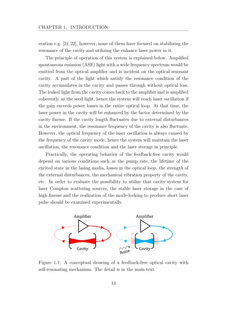
anism” was proposed by Y. Honda and K. Sakaue in 2010 [20]. Figure 1.1
shows a conceptual drawing of the feedback-free cavity with self-resonating
mechanism. Since it is composed of an optical amplifier and an optical
resonant cavity through optical loop pass, it also can be regarded as a kind
of laser oscillator. Laser oscillators including optical resonator (or etalon)
in the loop path has been widely used as a technique to stabilize laser op-
13
CHAPTER 1. INTRODUCTION
eration e.g. [21, 22], however, none of them have focused on stabilizing the
resonance of the cavity and utilizing the enhance laser power in it.
The principle of operation of this system is explained below. Amplified
spontaneous emission (ASE) light with a wide frequency spectrum would be
emitted from the optical amplifier and is incident on the optical resonant
cavity. A part of the light which satisfy the resonance condition of the
cavity accumulates in the cavity and passes through without optical loss.
The leaked light from the cavity comes back to the amplifier and is amplified
coherently as the seed light, hence the system will reach laser oscillation if
the gain exceeds power losses in the entire optical loop. At that time, the
laser power in the cavity will be enhanced by the factor determined by the
cavity finesse. If the cavity length fluctuates due to external disturbances
in the environment, the resonance frequency of the cavity is also fluctuate.
However, the optical frequency of the laser oscillation is always caused by
the frequency of the cavity mode, hence the system will maintain the laser
oscillation, the resonance condition and the laser storage in principle.
Practically, the operating behavior of the feedback-free cavity would
depend on various conditions such as the pump rate, the lifetime of the
excited state in the lasing media, losses in the optical loop, the strength of
the external disturbances, the mechanical vibration property of the cavity,
etc. In order to evaluate the possibility to utilize that cavity system for
laser Compton scattering sources, the stable laser storage in the case of
high finesse and the realization of the mode-locking to produce short laser
pulse should be examined experimentally.
Figure 1.1: A conceptual drawing of a feedback-free optical cavity with
self-resonating mechanism. The detail is in the main text.
14

CHAPTER 1. INTRODUCTION
1.3 Focus of Dissertation
In this thesis, the development of a feedback-free optical resonant cavity
with high finesse (394,000) in continuous oscillation operation is introduced.
That finesse is two orders of magnitude higher than one of our previous
performance. Thanks to the self-resonant mechanism, the demonstration
of maintaining the resonance was proven successfully even without high
precision electronic circuits or special quiet environment.
In order to provide basic knowledge about a laser Compton scattering
source, an optical power enhancement cavity and a laser oscillator, the
theoretical background is introduced in Chapter 2. High quality optical
mirrors enabling the large power enhancement and evaluation methods of
performance of the cavity are introduced in Chapter 3. Chapter 4 shows the
results of the principle verification experiment using a low finesse cavity and
the demonstration of the stable laser storage with the power enhancement
factor of mort than 100,000. Chapter 5 is a conclusion of this thesis.
15

Chapter 2
Theoretical backgrounds
2.1 Laser Compton scattering and scattered
photon beam
The laser Compton scattering means Compton scattering process with laser
photons and high energy electrons. The laser photon energy is around
visible range of O(1) eV while the electron have relativistic energy. Many
theoretical studies and numerical simulations for light sources using the
laser Compton scattering have been conducted so far (e.g. [23–26]). In this
section, the characteristics of scattered photons due to Compton scattering
are introduced; where by taking account the photon energy range of many
practical X-ray or gamma-ray sources, the recoil effect has been neglected.
2.1.1 Photon generation by Compton scattering
Consider an electron and a photon in a laboratory frame coordinate system
(x, y, z) as shown in the geometry of the scattering, figure 2.1. The 4-
momenta of the initial and final electrons are defined as p = (Ee/c, p)
and p′ = (E ′e/c, p′), where c is the speed of light. The initial electron is
moving along the z direction. The 4-momenta of the incident and scattered
photons are defined as k = (Ep/c, !k) and k′ = (E ′p/c, !k′), where ! is
the Planck constant. The incident photon is propagated along the direction
with the elevation angle θi and azimuth angle φi, and the scattered photon
16

CHAPTER 2. THEORETICAL BACKGROUNDS
Figure 2.1: Geometry of Compton scattering in a laboratory frame coor-
dinate system (x, y, z). The final electron p′ which is the electron after
scattering is not shown in this figure. The detail is in the main text.
is propagated along the direction with θs and φs. The angle θp (= θi − θs)
in figure 2.1 is the angle between the momenta of the incident and scattered
photons.
The energy of the scattered photon can be obtained from the kinematic
relation between the electrons and photons:
p+ k = p′ + k′. (2.1.1)
Squaring both side of this equation, we can obtain
E ′p =
1− β cos θi1− β cos θs + ε(1− cos θp)
Ep, (2.1.2)
where β = v/c, v is the velocity of the initial electron, and ε is the ratio
between the energies of the initial electron and the incident photon:
ε =Ep
Ee. (2.1.3)
Figure 2.2 shows the relation between the scattered photon energy and the
scattering angle with the incident angle of 180 (line), 120 (dash) and 90
(dots). The scattered angle θs is normalized with a factor of γ; position 1 on
the horizontal axis shows the scattered angle of θs = 1/γ [rad]. Those plots
are calculated with the electron energy of 1.28 GeV and the wavelength of
the incident laser of 1064 nm. It is found that the higher energy photons are
17

CHAPTER 2. THEORETICAL BACKGROUNDS
Figure 2.2: Scattered photon energy as a function of the scattered angle.
The electron energy and the wavelength of the incident laser are 1.28 GeV
and 1064 nm, respectively. Each curve correspond to the incident angle of
180 (line), 120 (dash) and 90 (dots).
concentrated around the axis of the electron propagation, θs = 0, regardless
of the incident angle.
In the head-on collision case, θi = π, equation (2.1.2) can be rewritten
as
E ′p =
1 + β
1− β cos θs + ε(1 + cos θs)Ep. (2.1.4)
Furthermore, assuming that the electron’s velocity is almost close to the
speed of light, the scattered photon energy in a small scattered angle, θs ≪1, is given by
E ′p =
4γ2
1 + 4γ2εEp, (2.1.5)
where γ = 1/√
1− β2 is the Lorentz factor of the initial electron. Neglect-
ing the recoil effect is a good assumption for practical applications of X-ray
or relatively low energy gamma-ray sources: 4γ2ε ≪ 1. Taking account
these assumption, the approximate maximum energy of scattered photons
is given by
E ′p ∼ 4γ2Ep. (2.1.6)
18
CHAPTER 2. THEORETICAL BACKGROUNDS
This result shows that the incident photon is boosted by a factor of about
γ2. Since the Lorentz factor of the electron γ is much bigger than unity in
the ultra-relativistic case, the laser Compton scattering using an electron
accelerator can be utilized to produce high-energy photons even though
laser photons are only O(1) eV energy.
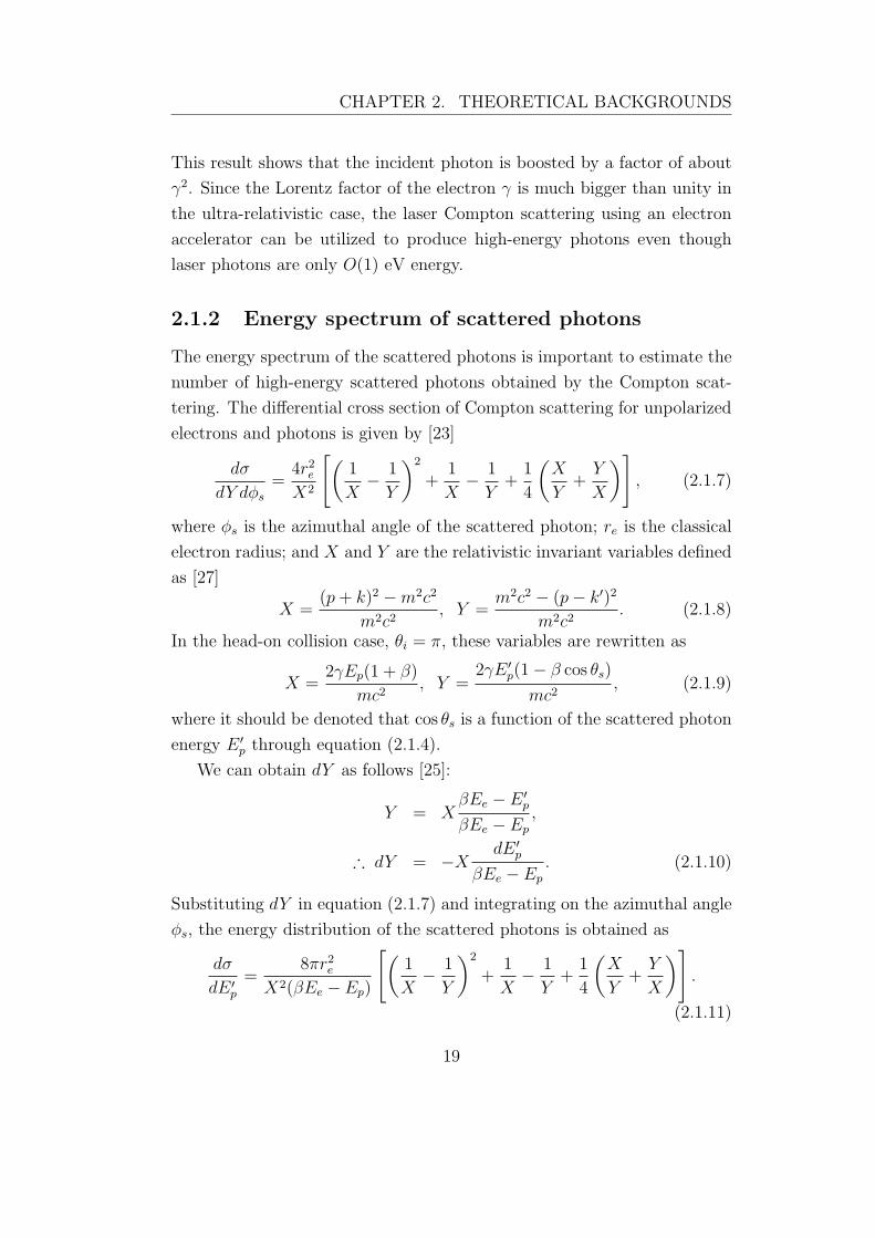
2.1.2 Energy spectrum of scattered photons
The energy spectrum of the scattered photons is important to estimate the
number of high-energy scattered photons obtained by the Compton scat-
tering. The differential cross section of Compton scattering for unpolarized
electrons and photons is given by [23]
dσ
dY dφs=
4r2eX2
[(1
X− 1
Y
)2
+1
X− 1
Y+
1
4
(X
Y+
Y
X
)], (2.1.7)
where φs is the azimuthal angle of the scattered photon; re is the classical
electron radius; and X and Y are the relativistic invariant variables defined
as [27]
X =(p+ k)2 −m2c2
m2c2, Y =
m2c2 − (p− k′)2
m2c2. (2.1.8)
In the head-on collision case, θi = π, these variables are rewritten as
X =2γEp(1 + β)
mc2, Y =
2γE ′p(1− β cos θs)
mc2, (2.1.9)
where it should be denoted that cos θs is a function of the scattered photon
energy E ′p through equation (2.1.4).
We can obtain dY as follows [25]:
Y = XβEe − E ′
p
βEe − Ep,
∴ dY = −XdE ′
p
βEe − Ep. (2.1.10)
Substituting dY in equation (2.1.7) and integrating on the azimuthal angle
φs, the energy distribution of the scattered photons is obtained as
dσ
dE ′p
=8πr2e
X2(βEe − Ep)
[(1
X− 1
Y
)2
+1
X− 1
Y+
1
4
(X
Y+
Y
X
)].
(2.1.11)
19

CHAPTER 2. THEORETICAL BACKGROUNDS
Figure 2.3: The energy spectrum of the scattered photons by Compton
scattering with the electron energy of 1.28 GeV and the laser wavelength
of 1064 nm.
The energy spectrum of the scattered photons with the electron energy of
1.28 GeV and the laser wavelength of 1064 nm is shown in figure 2.3. The
spectral intensity has a maximum value at the scattered photon energy of
about 29 MeV, which is the maximum energy obtained at the scattered
angle of θs = 0. And a minimum value at the scattered photon energy of
about 15 MeV, that energy is obtained at the scattered angle of θs = 1/γ
according to the angular distribution of the scattered photon energy, figure
2.2. Thus, a half of power of the scattered photons will be concentrated in
a cone of the angle θs = 1/γ = 0.399 [mrad]. The results indicates that
we can obtain a high-energy scattered photon beam with a small energy
spread by using collimators at downstream of the interaction area.
2.1.3 Flux of a scattered photon beam
To obtain the expression for the total flux of the scattered photons, consider
the beam-beam scattering of the electrons and laser photons. Figure 2.4
shows the collision of a bunched electron beam and a pulsed laser beam in a
laboratory frame coordinate system (x, y, z). The electron bunch is moving
20
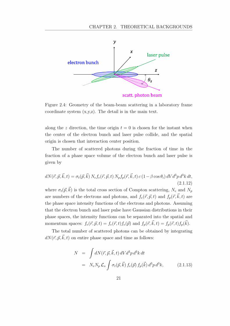
CHAPTER 2. THEORETICAL BACKGROUNDS
Figure 2.4: Geometry of the beam-beam scattering in a laboratory frame
coordinate system (x,y,z). The detail is in the main text.
along the z direction, the time origin t = 0 is chosen for the instant when
the center of the electron bunch and laser pulse collide, and the spatial
origin is chosen that interaction center position.
The number of scattered photons during the fraction of time in the
fraction of a phase space volume of the electron bunch and laser pulse is
given by
dN(r, p, k, t) = σt(p, k)Nefe(r, p, t)Npfp(r, k, t) c (1−β cos θi) dV d3p d3k dt,
(2.1.12)
where σt(p, k) is the total cross section of Compton scattering, Ne and Np
are numbers of the electrons and photons, and fe(r, p, t) and fp(r, k, t) are
the phase space intensity functions of the electrons and photons. Assuming
that the electron bunch and laser pulse have Gaussian distributions in their
phase spaces, the intensity functions can be separated into the spatial and
momentum spaces: fe(r, p, t) = fe(r, t)fe(p) and fp(r, k, t) = fp(r, t)fp(k).
The total number of scattered photons can be obtained by integrating
dN(r, p, k, t) on entire phase space and time as follows:
N =
∫dN(r, p, k, t) dV d3p d3k dt
= NeNp Ls
∫σt(p, k) fe(p) fp(k) d
3p d3k, (2.1.13)
21

CHAPTER 2. THEORETICAL BACKGROUNDS
where
Ls = c (1− β cos θi)
∫fe(r, t) fp(r, t) dV dt (2.1.14)
is the single-collision luminosity defined as the number of events produced
per unit cross section of the scattering [25]. In the head-on collision case,
θi = π, with relativistic electrons of β ∼ 1, that luminosity is rewritten as
Ls =1
2π
(λzR4π
+ βxϵx
)− 12(λzR4π
+ βyϵy
)− 12
, (2.1.15)
where λ is the laser wavelength, zR is the Rayleigh range, βx,y are Twiss
parameters of the electron beam, and ϵx,y are transverse emittance. As a
conclusion, the total number of scattered photons in unit time is given by
dN
dt= fNeNpLsσt, (2.1.16)
where f is the repetition rate of the collision, σt is the averaged total cross
section of Compton scattering; it can be approximated by σt when the
energy spread of the electrons and laser photons are neglected. This ex-
pression shows that as the laser power increasing the flux of the scattered
photon beam increases proportionally.
2.2 Principle of an optical resonant cavity
An optical resonant cavity is a device that realizes power storage of laser
light; when the cavity resonates with incident laser light, the light accu-
mulates coherently in the cavity. The power enhancement factor of the
laser storage is expressed by the power reflectivity R of the cavity mirror:
1/(1 − R). By constructing the cavity with high reflectivity mirrors, the
large enhancement factor can be obtained, however, there is a problem that
coherence collapses with slight phase change. In order to think about this
problem, this section explains the principle of the optical resonant cavity.
(For the spatial characteristics of the cavity, see Appendix A.)
22

CHAPTER 2. THEORETICAL BACKGROUNDS
2.2.1 Transmitted and reflected light of a Fabry-Perot
cavity
Figure 2.5 shows the most basic optical resonant cavity which consists of
two concave mirrors (Fabry-Perot cavity) [28]. When the input mirror (M1)
of the cavity is irradiated with the incident laser light, a part of the light
field goes through the mirror by the transmission coefficient t1. The light in
the cavity undergoes a change in amplitude by each round-trip with a factor
of the reflection coefficient of cavity mirrors: r1 and r2. On the other hand,
a part of the laser light inside the cavity exit from both the input (M1) and
output (M2) cavity mirrors by each round-trip. Thus, the reflected light by
the cavity is expressed by the superposition of the prompt reflection of the
incident light and penetrations from the cavity, while the transmitted light
is the superposition of the penetrations from the cavity.
The transmitted and reflected light fields (electric fields) Etr(t) and
Ere(t) are given by [29]
Ein(t) = E0eiωt, (2.2.1)
Etr(t) = E0eiωt[t1t2e
−iω lc + t1t2r1r2e
−iω 3lc + · · ·
], (2.2.2)
Ere(t) = E0eiωt[r1 − r2t
21e
−iω 2lc − r1r
22t
21e
−iω 4lc − · · ·
], (2.2.3)
where l is the cavity length (the distance between two mirrors), c is the
speed of light, and t1,2 are transmission coefficients of the cavity mirrors,
respectively. The factor e−iω 2lc indicates the phase shift for each round-trip
Figure 2.5: A conceptual drawing of a Fabry-Perot cavity with the cavity
length l. r1,2 and t1,2 are reflection and transmission coefficients, and R1,2
and T1,2 are intensity reflectivity and transmittance of the cavity mirrors.
23

CHAPTER 2. THEORETICAL BACKGROUNDS
of the light in the cavity. From infinite series of those equations, the transfer
functions of the cavity are given by
Etr
Ein=
t1t2e−iω lc
1− r1r2e−2iω lc
, (2.2.4)
Ere
Ein=
r1 − r2(r21 + t21)e−2iω l
c
1− r1r2e−2iω lc
. (2.2.5)
For later use, another derivation method is shown in figure 2.6 [30, 31].
The transmitted field is derived by using the forward-going field EF (t) and
the backward-going field EB(t); these fields are given by
EF (t) = t1Ein(t)− r1EB(t− T )e−iωT , (2.2.6)
EB(t) = −r2EF (t− T )e−iωT , (2.2.7)
where T = 2l/c is the one round-trip time of the intra-cavity light. Substi-
tuting equation (2.2.7) to equation (2.2.6), the forward-going field is rewrit-
ten as
EF (t) = t1Ein(t) + r1r2EF (t− T )e−iωT . (2.2.8)
Assuming that the intra-cavity field settles down to the stead-state con-
dition, we obtain the relation of EF (t) = EF (t − T ). Therefore, equation
(2.2.8) can be solved as
EF (t) =t1
1− r1r2e−iωTEin(t). (2.2.9)
Figure 2.6: The conceptual drawing of the self-consistent scheme to intro-
duce the transmitted light field from the cavity. EF (t) is the forward-going
field and EB(t) the backward-going field.
24

CHAPTER 2. THEORETICAL BACKGROUNDS
By multiplying the transmission coefficient t2, the transmitted field from
the cavity is obtained as follows:
Etr(t) =t1t2e−iωT/2
1− r1r2e−iωTEin(t). (2.2.10)
2.2.2 Transfer functions of a Fabry-Perot cavity and
the cavity finesse
Assuming that two cavity mirrors have same intensity transmittance and
reflectivity, T1 = T2 = T and R1 = R2 = R, the transfer functions for the
transmitted and reflected light intensities are given by
ItrIin
=
∣∣∣∣Etr
Ein
∣∣∣∣2
=T 2
(1−R)2 + 4R sin2 (ω/2νFSR), (2.2.11)
IreIin
=
∣∣∣∣Ere
Ein
∣∣∣∣2
=R[A2 + 4(R + T ) sin2 (ω/2νFSR)
]
(1−R)2 + 4R sin2 (ω/2νFSR), (2.2.12)
where R and T have the relations as follows:
Ri = r2i , (2.2.13)
Ti = t2i ; (2.2.14)
A is the optical loss coefficient defined as
A = 1−R− T ; (2.2.15)
νFSR is the free spectrum range of the cavity defined by
νFSR =c
2l. (2.2.16)
From equation (2.2.11) and (2.2.12), it is found that the cavity resonates
with the incident light under the resonant condition:
ω
2νFSR=
2πν
2νFSR= qπ, (2.2.17)
where ν is the optical frequency of the incident light, q is an integer called
the mode number. The resonance condition can be also written as the
relation of the wavelength λ and the cavity length l:
l =λ
2q. (2.2.18)
25

CHAPTER 2. THEORETICAL BACKGROUNDS
Figure 2.7: The transmitted light intensity with several reflectivities of the
cavity mirrors. The transmitted intensity on the resonance condition equals
the incident intensity in the case of without the optical loss on the mirrors.
Figure 2.7 and 2.8 show equation (2.2.11) and (2.2.12) as a function of
ν with several R under the condition of A = 0. It is found that curves have
resonance peaks (or dips) with a period of νFSR and the linewidth of the
peak narrows as the reflectivity of the mirror approaches unity.
When the light frequency changes slightly by δν around the resonance
frequency, the denominator on the right side of equation (2.2.11) can be
rewritten as
(1−R)2 + 4R sin2
(2πδν
2νFSR
)∼ (1−R)2 + 4R
(πδν
νFSR
)2
. (2.2.19)
From this relation, the full width at the half maximum (FWHM) of the
resonant peak, ∆ν, can be calculated as follows:
(1−R)2 + 4R
(π
νFSR
∆ν
2
)2
= 2(1−R)2
(∆ν
2
)2
=(1−R)2
4π2Rν2FSR
∆ν =1−R
π√RνFSR. (2.2.20)
From this expression, the sharpness of the resonance peak can be defined as
an important parameter of the cavity called finesse, which is also known as a
guide of the resolution of an optical spectrum analyzer using a Fabry-Perot
26
CHAPTER 2. THEORETICAL BACKGROUNDS
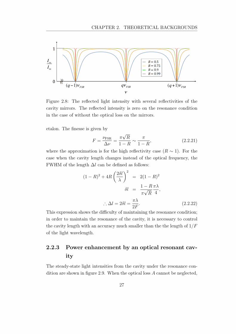
Figure 2.8: The reflected light intensity with several reflectivities of the
cavity mirrors. The reflected intensity is zero on the resonance condition
in the case of without the optical loss on the mirrors.
etalon. The finesse is given by
F =νFSR∆ν
=π√R
1−R∼ π
1−R, (2.2.21)
where the approximation is for the high reflectivity case (R ∼ 1). For the
case when the cavity length changes instead of the optical frequency, the
FWHM of the length ∆l can be defined as follows:
(1−R)2 + 4R
(2δl
λ
)2
= 2(1−R)2
δl =1−R
π√R
πλ
4,
∴ ∆l = 2δl =πλ
2F. (2.2.22)
This expression shows the difficulty of maintaining the resonance condition;
in order to maintain the resonance of the cavity, it is necessary to control
the cavity length with an accuracy much smaller than the the length of 1/F
of the light wavelength.
2.2.3 Power enhancement by an optical resonant cav-
ity
The steady-state light intensities from the cavity under the resonance con-
dition are shown in figure 2.9. When the optical loss A cannot be neglected,
27

CHAPTER 2. THEORETICAL BACKGROUNDS
the transmitted intensity is smaller than the incident light and the reflected
intensity does not become zero. The intra-cavity intensity Icav is given by
Icav =2T
(1−R)2Iin, (2.2.23)
where the indicated factor of 2 means that the light forms a standing wave
in the cavity, and the coefficient 2T/(1 − R)2 indicates the enhancement
factor of the light power. In the case of T = 1−R, the enhancement factor
G will be proportional to the finesse or simply 1−R:
G =2T
(1−R)2=
2
1−R∼ 2F
π. (2.2.24)
It should be noted that the enhancement factor G is not only the power
enhancement factor but also the factor for the interaction length of intra-
cavity light.
2.2.4 Lifetime of the light inside the cavity
When the incident light is removed at t = t0, the light power stored in
the cavity decreases due to the transmission and the optical loss. In times
t > t0, the forward-going field in the cavity shown in equation (2.2.8) is
given by
EF (t+2l
c) = REF (t), (2.2.25)
where we can neglect the exponential factor since the cavity had been res-
onated until the time t < t0. With the Taylor series approximation, the
Figure 2.9: The steady-state intensities around the cavity at the resonance
condition. The light power inside the cavity is enhanced by a magnitude of
about the finesse.
28

CHAPTER 2. THEORETICAL BACKGROUNDS
left-hand side of equation (2.2.25) is rewritten as
EF (t+2l
c) ∼ EF (t) +
2l
c
d
dtEF (t). (2.2.26)
Thus, the differential equation for the forward-going field is obtained:
d
dtEF (t) = − c
2l(1−R)EF (t). (2.2.27)
The solutions of this differential equation and the forward-going intensity
are calculated as follows:
EF (t) = EF (t0) exp[− c
2l(1−R)(t− t0)
], (2.2.28)
IF (t) = |EF (t)|2 = IF (t0) exp
[−(t− t0)
τc
], (2.2.29)
where the decay time constant τc is given by
τc =l
c(1−R)∼ l
πcF =
1
2π∆ν. (2.2.30)
This decay time constant indicates the lifetime of the light inside the cavity
and is the inverse of the resonance linewidth ∆ν. As will later be shown,
measuring the lifetime of the intra-cavity light is an effective means for
obtaining the cavity finesse.
2.3 Laser amplifier and oscillator
The principle of the feedback-free optical cavity is based on a ring laser
oscillator; an optical resonant cavity is added as the storage cavity to the
circulating optical path of the oscillator. In this experiment, we used an
ytterbium-doped fiber amplifier (YDFA) which is known to operate as the
almost four-level laser system [34]. In order to understand the transfer of
energy between the amplifier, the laser cavity which is the circulating optical
path and the storage cavity, the principle of a four-level laser system and the
dynamic characteristics of laser oscillators are introduced in this section.
29

CHAPTER 2. THEORETICAL BACKGROUNDS
2.3.1 Four-level laser system
A four-level laser system consists of the ground level (0), the lower level
of the laser transition (1), the upper level of the laser transition (2) and
the excitation band (3) as shown in figure 2.10. Here, the atoms (doped
ions of rare-earth metal in silica glass material) are excited from (0) to
(3) by the light pumping process, and transition from (2) to (1) while
coherently amplifying signal light. Ni (i = 0, 1, 2, 3) are occupation numbers
or population of the atoms [number/m3] at each level. The population
inversion associated with laser transition can be denoted as N2 − N1. In
the ideal four-level system, since the transition from (1) to (0) and the
transition from (3) to (2) are very fast transitions, we can neglect those
population: N1 = N3 = 0. Furthermore, the population inversion can be
rewritten as N2 −N1 = N2.
In order to describe transitions of the atoms each level, we use the stim-
ulated transition rate W (ν) [1/s] and the spontaneous emission transition
rate γ2 [1/s], where ν is optical frequency and γ2 is the inverse of the fluo-
rescence lifetime τ2 of the level (2):
γ2 =1
τ2. (2.3.1)
The time variation of the population inversion which is known as the rate
equation is given by [32]
dN2
dt= (Nt −N2)Wp(νp)− γ2N2 −N2Ws(νs), (2.3.2)
Figure 2.10: An energy level diagram of a four-level system. Details are in
the main text.
30

CHAPTER 2. THEORETICAL BACKGROUNDS
Figure 2.11: Absorption and emission cross sections of a ytterbium-doped
optical fiber. The data is from [34].
where the subscripts p, s indicate the pump light and signal light that we
want to amplify; each term are corresponding to the pumping, spontaneous
emission and stimulated emission process in order from the left, respectively.
The transition rate of the pumping process is proportional to the ground
level populatio, N0 (= Nt −N2), where Nt is the total number of atoms in
the unit volume.
The stimulated transition rate W (ν) are expressed as follows:
W (ν) =σem(ab)
hνΓI, (2.3.3)
where σem(ab) is the stimulated emission (or absorption) cross section [m2]; I
is the light intensity [W/m2]; Γ is the spatial overlapping coefficient between
the light and the laser medium; hν is the photon energy [J], where h is
Plank’s constant. Using this expression, the rate equation is rewritten as
dN2
dt= (Nt −N2)
σab
hνpΓpIp − γ2N2 −N2
σem
hνsΓsIs. (2.3.4)
For accurate analysis, the rate terms should be integrated over a range
of optical frequencies from zero to infinity since the pump and signal lights
have the finite linewidth. Furthermore, the absorption and emission cross
31

CHAPTER 2. THEORETICAL BACKGROUNDS
sections of a ytterbium-doped optical fiber, figure 2.11, shows that both
spectra overlap in wide wavelength range; in many cases, the wavelength of
the pump light is chosen at 915 nm or 976 nm; the amplifiable wavelength
band of the YDFA is in the range of 1020 nm to 1070 nm because the
emission cross section is larger than the absorption cross section in that
range. The rate equation can be modified as follows [33]:
dN2
dt=
∫ ∞
0
I(ν)
hνΓ [(Nt −N2)σab −N2σem] dν − γ2N2. (2.3.5)
It is not necessary to use this equation when the pump and signal lights are
approximated to monochromatic. Analysis of the amplified spontaneous
emission (ASE) in fiber amplifiers, for example, require such a detailed
expression.
2.3.2 Equations of the light propagation
The light power generated per unit volume [W/m3] by the stimulated emis-
sion process is given by
N2Ws(νs)× hνs = N2σemΓsIs. (2.3.6)
This additional optical power is coherent to the incident signal light, so
the intensity of the signal is amplified along the propagation direction z
according to the following differential equation:
dIsdz
= ΓsN2σemIs. (2.3.7)
Similarly, we obtain the following differential equation for the absorption
process of the pump light:
dIpdz
= Γp(Nt −N2)σabIp. (2.3.8)
In the case of a fiber amplifier, there are two directions of light prop-
agation. Consider the traveling direction of the signal light is taken as
the forward direction, the differential equations for the two propagation
directions of the pump light are given by
±dI±pdz
= Γp(Nt −N2)σabI±p , (2.3.9)
32

CHAPTER 2. THEORETICAL BACKGROUNDS
where superscripts + and − indicate the forward and backward directions,
respectively. In generally, there are three schemes of the optical pumping for
fiber amplifiers: the forward pumping, backward pumping and the double-
side pumping. This two-directions analysis is also essential for analysis of
the ASE [33].
2.3.3 Steady-state behavior of a laser oscillator
Consider a laser oscillator consisting of an amplifier and a laser cavity which
is an arbitrary optical feedback path. For simplicity, the rate equation
(2.3.4) is rewritten as
dN2
dt= Rp − γ2N2 −KN2q, (2.3.10)
where
Rp = Ntσab
hνpΓpIp, (2.3.11)
K = σemΓs, (2.3.12)
and
q =Ishνs
(2.3.13)
is the photon number density [number/m2]. The pumping term is replaced
by the constant Rp assuming that the steady state population inversion is
much smaller than the ground level population: Nt − N2 ∼ Nt. The rate
equation for the photon number is given by
dq
dt= KN2q − γLq, (2.3.14)
where γL is the photon decay rate of the laser cavity; it defined by optical
loss and the traveling time in the cavity:
γL =− lnαloop
τL, (2.3.15)
where αloop is the optical loss in one round-trip pass in the laser cavity, and
τL is the decay time constant of the laser cavity.
33

CHAPTER 2. THEORETICAL BACKGROUNDS
Figure 2.12: The steady state behavior of a laser oscillator. r = 1 is the
threshold of the laser oscillation. Details are in the main text
The threshold condition of the laser oscillation is obtained by calculating
the steady-state population inversion N ss2 and the photon number qss. From
equation (2.3.10), the steady-state condition is
0 = Rp − γ2N2 −KN2q,
∴ N ss2 =
Rp
γ2 +Kqss. (2.3.16)
From equation (2.3.14), the steady-state condition is also
0 = KN ss2 qss − γLq
ss
= (KN ss2 − γL)q
ss,
∴
⎧⎨
⎩qss = 0
N ss2 = γL/K
. (2.3.17)
Substituting the solution of N ss2 for equation (2.3.16), another solution of
the steady state photon number is obtained as
qss =Rp
γL− γ2
K. (2.3.18)
Taking into account the solution qss = 0, the threshold pumping rate for
laser oscillation, Rthp , is obtained as
Rthp =
γ2γLK
. (2.3.19)
34

CHAPTER 2. THEORETICAL BACKGROUNDS
With this threshold pumping rate, we defined the pump ratio r as follows:
r ≡ Rp
Rthp
=K
γ2γLRp. (2.3.20)
The steady state behavior is distinguished into two situations at the thresh-
old r = 1 as shown in figure 2.12. When r < 0, the population inversion
increases in proportion to the pump rate and the laser oscillation does not
build up (qss = 0). When r > 0, the population inversion is saturated at
N ss2 = γL/K and the number of laser photons simply increases in proportion
to the pump rate.
2.3.4 Relaxation oscillations
When the laser oscillation is perturbed from its steady state, spiking and
damped oscillations occur. Such behavior is well known as relaxation os-
cillations [35] and described by two differential equations of the population
inversion equation (2.3.10) and the photon number equation (2.3.14). Those
equations, however, can not be analytically solved due to the coupled term
of KN2q. Thus, we carry out a linearized analysis and introduce simple
analytic solutions for relaxation oscillations.
Let’s consider small perturbations of N2 and q from their steady state
values as follows:
N2 = N ss2 +∆N, (2.3.21)
q = qss +∆q, (2.3.22)
where ∆N ≪ N ss2 and ∆q ≪ qss. Substituting these in equations (2.3.10)
and (2.3.14), and neglecting the coupling term ∆N∆q, the following equa-
35

CHAPTER 2. THEORETICAL BACKGROUNDS
tions for ∆N and ∆q are obtained:
d∆N
dt= Rp − γ2(N
ss2 +∆N)−K(N ss
2 +∆N)(qss +∆q)
= Rp − γ2Nss2 −KN ss
2 qss − γ2∆N −KN ss2 ∆q −Kqss∆N
−K∆N∆q
= −γ2∆N −KN ss2 ∆q −Kqss∆N
= −γ2∆N − γL∆q − (r − 1)γ2∆N
= −γL∆q − rγ2∆N, (2.3.23)d∆q
dt= K(N ss
2 +∆N)(qss +∆q)− γL(qss +∆q)
= KN ss2 qss − γLq
ss +KN ss2 ∆q +Kqss∆N − γL∆q +K∆N∆q
= −γ2∆N +KN ss2 ∆q −Kqss∆N
= γL∆q + (r − 1)γ2∆N − γL∆q
= (r − 1)γ2∆N, (2.3.24)
where relations N ss2 = γL/K and qss = (r−1)γ2/K are used. By differenti-
ating equation (2.3.24) with respect to time, and using equation (2.3.23) to
eliminate ∆N from the resulting equation, the linearized equation for ∆q
is obtained as
d2∆q
dt2+ rγ2
d∆q
dt+ (r − 1)γ2γL∆q = 0. (2.3.25)
The equation (2.3.25) is the second-order system with the natural angular
frequency ωn and the damping ratio ζ given by
ωn =√
(r − 1)γ2γL, (2.3.26)
ζ =rγ22ωn
=r
2√r − 1
(γ2γL
) 12
. (2.3.27)
When the steady state light intensity is perturbed, the exponentially
damped oscillations occur with the angular frequency of
ωro = ωn
√1− ζ2 (2.3.28)
and the decay time constant of
τro =2
rγ2. (2.3.29)
36

CHAPTER 2. THEORETICAL BACKGROUNDS
The behavior of relaxation oscillations depends on the relative size of the
decay rates γ2 and γL. In most gas lasers, its atomic fluorescence lifetime is
short and the cavity decay time constant is relatively long due to its long
cavity length; γ2 and γL are of same order of magnitude: γ2 ∼ γL. Since
the damping ratio ζ is almost unity, the laser intensity behaves non-spiking
relaxation oscillations. On the other hand, most semiconductor lasers and
many solid-state lasers indicate the very much slower atomic decay rate
compared to the cavity decay rate: γ2 ≪ γL. Such lasers show the strong
spiking on relaxation oscillations owing to their small damping ratio. The
time period of the spiking Tro is given by Tro = 2π/ωro or Tro = 2π/ωn
because ζ2 term in equation (2.3.28) can be neglect.
37

Chapter 3
Ultra-low loss mirrors and
finesse measurement
techniques
3.1 Ultra-low loss mirrors
One of the most fundamental ploblems to develop a high finesse optical
resonant cavity is the gaining quality of the cavity mirrors. An optical mir-
ror is characterized by three parameters which satisfy the relation (2.2.15):
the intensity reflectance R, transmittance T and loss coefficient A. The
reflectance and transmittance are determined by a design of the reflection
coating on a substrate of the mirror. The intensity loss is caused by the
scattering and absorption on the surface of the coat and substrate. The
achieving loss is limited by the manufacturing accuracy of the mirror; only
a few companies can produce an ultra-low loss mirror with less than ppm
(= 10−6) loss coefficient [36].
Since the surface condition of such high quality mirror can easily get de-
teriorated by contamination, one must handle it carefully. Additional loss
decreases the cavity finesse, and the absorption loss will be become a prob-
lems in the application of high power lasers because of thermal deformation
of the mirror. Thus, studies on handling method of ultra-low loss mirrors
are also important in the development of high finesse cavity systems.
38

CHAPTER 3. ULTRA-LOW LOSS MIRRORS AND FINESSEMEASUREMENT TECHNIQUES
Ultra-low loss mirrors are manufactured by the dielectric multilayer
coating, which is formed by depositing high refractive index material and
low refractive index material on a glass substrate alternately. The ion-beam
sputtering process is widely applied to form the multilayer coating since it
can make dense coats with low roughness; the scattering loss of an optical
mirror mainly depends on the roughness of the glass substrate. The surface
roughness is characterized by the total integrated scattering (TIS) which is
related to the root-mean-square of the roughness δ [37]:
TIS =
(4πδ
λ
)2
. (3.1.1)
This equation indicates that the angstrom roughness is required to realize
the ppm-order scattering loss with visible to near-infrared wavelength range.
3.2 Scattering loss measurement and han-
dling of the mirror
Figure 3.1: The optical setup of the scatter meter at TAMA experimental
hall in National Astronomical Observatory of Japan (NAOJ) [37]. It can
measure the 2-dimensional map of the TIS on a mirror surface.
39

CHAPTER 3. ULTRA-LOW LOSS MIRRORS AND FINESSEMEASUREMENT TECHNIQUES
Figure 3.2: Measurement results of the scattering losses of our ultra-low
loss mirrors. Those values had systematic errors of a few ppm.
In order to evaluate the performance of our low loss mirrors, we mea-
sured the scattering loss of those by using the scatter meter in National
Astronomical Observatory of Japan (NAOJ) [37]. The optical setup of the
measurement is shown in figure 3.1. The incident laser light was shaped
in the fundamental Gaussian mode by a pinhole filter and flushed on the
measured mirror surface. While the laser irradiated on the flat surface area
of the mirror was reflected back to the incident trajectory, scattered light
at the rough mirror surface was lead to a photo-diode detector by the inte-
grated sphere. The scattered light intensity was measured by scanning the
position of the mirror by a x-y stage. Here, the incident laser was switched
on/off by an acousto-optic modulator with the intensity modulation of 1
MHz in order to improve the signal-to-noise ratio.
The ultra-low loss mirrors were flat mirrors with the diameter of 25.4
mm. Those mirrors were provided from two suppliers; one of them was
Laboratoire Materiaux Avances (LMA, France) and their mirrors had the
reflectivity of about 99.999 % according to the specification; another sup-
plier was Advanced Thin Films (ATF, USA) and their mirrors had the loss
coefficient of as low as 1 ppm according to the specification. Figure 3.2
shows measurement results of the scattering losses at the central area of 1
cm2 on each mirror surface, where mirrors were referred as ATF#1, ATF#2
and LMA. The obtained averaged scattering losses were 25.0 ppm, 8.1 ppm
and 12.9 ppm for ATF#1, ATF#2 and LMA, respectively, where value un-
certainty was a few ppm. We found that the mirror labeled ATF#1 had
practically large scattering losses and that value was far from its specifica-
40

CHAPTER 3. ULTRA-LOW LOSS MIRRORS AND FINESSEMEASUREMENT TECHNIQUES
Figure 3.3: A schematic drawing of the drag-wiping technique. The detail
is described in the main text or [38].
Figure 3.4: Measured scattering losses after the cleaning by the drag-wiping
technique. The scattering losses of other mirrors were also improved by
cleaning the mirror surfaces.
tion value.
In order to clean the contaminated mirror, ATF#1, we applied the
drag-wiping technique [38]. Figure 3.3 shows a schematic drawing of that
method. A cleaning paper is put on the mirror surface and a drop of pure
2-plopanol is applied on it. And then, the surface is wiped by dragging out
lens-cleaning papers. Figure 3.4 shows the scattering losses of ATF#1 after
the cleaning. The averaged scattering loss was improved from 25.0 ppm to
9.2 ppm with the minimum value of 4 ppm. Finally, all averaged scattering
losses were successfully improved from the values before the cleaning to less
than 10 ppm.
41

CHAPTER 3. ULTRA-LOW LOSS MIRRORS AND FINESSEMEASUREMENT TECHNIQUES
3.3 Finesse measurement techniques
There are several techniques to measure the cavity finesse depending on
the magnitude of the finesse. According to equation (2.2.21), the finesse
measurement means the measurement of the effective reflectivity of the
cavity mirrors. In this section, some typical methods are introduced.
3.3.1 Cavity ring-down technique
Figure 3.5: A schematic diagram of the cavity ring-down technique. AOM:
acousto-optic modulator, SMF: single mode fiber, FG: function genera-
tor, HV amp.: high-voltage amplifier, PZT: piezo electric transducer, PD:
photo-diode.
The time decay of the light in a Fabry-Perot cavity is given by equation
(2.2.29). Since the decay time constant is related to the cavity finesse and
the cavity length as shown in equation (2.2.30), the finesse can be obtained
by observing the time decay of the transmitted light from the cavity; this
method is called cavity ring-down technique.
A schematic diagram of the cavity ring-down technique is shown in figure
3.5. At the first, the optical cavity had been aligned with the fundamental
Gaussian mode of the incident laser light. The transmitted light from the
cavity was monitored while scanning the cavity length with a piezo-electric
transducer (PZT) actuator. When the cavity and the incident light closed
42

CHAPTER 3. ULTRA-LOW LOSS MIRRORS AND FINESSEMEASUREMENT TECHNIQUES
(a)(b)
Figure 3.6: (a) Observed time decay signal (cavity ring-down signal) by
using an oscilloscope. (b) The result of fitting with an exponential fit
function.
to the resonant condition, increase of the transmitted light power was ob-
served. Then, the incident light was shut-off by an acousto-optic modulator
(AOM) when the light power reached the certain threshold level.
The obtained data of the time decay signal, which is called as ring-down
signal, was fitted by an exponential function. An example of the measure-
ment results for the cavity consisting of ultra-low loss mirrors provided by
LMA is shown in figure 3.6a. The cavity length l was 0.216 ± 0.002 m
and the fall time of AOM was less than 4 µs. By fitting the data with an
exponential function as shown in figure 3.6b, the decay time constant τc,
finesse F and the corresponding effective reflectivity R were obtained as
τc = 60.21± 0.03 µs, F = 263, 000± 2, 000 and R = 99.99880± 0.00001 %,
respectively.
3.3.2 Sideband technique
When the magnitude of the cavity finesse is relatively low, the cavity ring-
down technique cannot be applied since the decay time constant is too
short to measure precisely. On the other hand, the cavity linewidth which
is inverse of the decay time becomes larger, thus the frequency-domain-
measurement technique known as sideband technique can be used. In this
method, frequency modulation is applied to the incident light to make side-
43

CHAPTER 3. ULTRA-LOW LOSS MIRRORS AND FINESSEMEASUREMENT TECHNIQUES
Figure 3.7: The setup diagram of the finesse measurement by the sideband
method. FI: Faraday isolator, FC: fiber coupler/collimator, HWP: half wave
plate, EOM: electro-optical modulator, PZT: piezo-electro transducer, PD:
photo detector, OSC: oscilloscope.
Figure 3.8: Measured resonance signal of the transmitted light. Small res-
onance signals at around the highest peak indicate the sideband lights.
band compornents as a frequency marker. Since the modulation frequency
can be well controlled, the linewidth is measured with good measurement
accuracy.
The setup diagram of the sideband method is shown in figure 3.7. FI is
a Faraday isolator, two FCs are single mode fiber collimator/coupler, HWP
is a half-wave plate, EOM is an electro-acoustic modulator, and PD is a
photo-diode detector, respectively. The cavity length l and the free spectral
range νFSR were 0.216 ± 0.002 m and 694.4 ± 6.4 MHz, respectively. The
expected finesse and linewidth were O(100) and O(1) MHz due to the mirror
reflectivity of 99.5 %, which is from the specification. The fundamental
Gaussian mode of the incident light was well aligned to the cavity by using
matching lens. And EOM gave 10 MHz sideband frequency to the incident
44

CHAPTER 3. ULTRA-LOW LOSS MIRRORS AND FINESSEMEASUREMENT TECHNIQUES
light.
Figure 3.8 shows the observed temporal signal of the transmitted light.
Since the cavity length was changed linear by using the PZT actuator, an
Airy function shape appeared as the resonance peak (refer figure 2.7). This
resonant peak was composed of the light with the carrier frequency which
was the original optical frequency of the incident laser. Since the laser
was modulated by EOM, the sidebands were observed at both sides of the
resonance of the carrier light. Here, the observed time distance between
the sideband and carrier peaks correspond to the modulation frequency
of 10 MHz. As a result, the cavity linewidth ∆ν, finesse F and effective
reflectivity R were obtained as ∆ν = 1.85 MHz, R = 375 ± 17 and R =
99.16± 0.04 %, respectively. The errors were mainly from the uncertainty
of the cavity length.
3.3.3 Frequency response function technique
The linewidth of the resonance peak can be evaluated by measuring the
cavity’s response function which means the frequency response around its
resonance frequency [39]. Figure 3.9 shows a conceptual scheme of this
method. By applying amplitude modulation to the incident laser with the
frequency Ω while the cavity is resonated at ω0, the frequency components
of ω0, ω0 −Ω and ω0 −Ω show up. The carrier light with the frequency ω0
passes through the cavity without any optical loss while the sidebands are
attenuated since those are off resonance with the phase difference of Ω.
Figure 3.9: A conceptual scheme of the frequency response function tech-
nique with intensity modulation. The detail is described in [39]
45

CHAPTER 3. ULTRA-LOW LOSS MIRRORS AND FINESSEMEASUREMENT TECHNIQUES
According to the reference [39], in the case of Ω/νFSR ≪ 1, the transfer
function for the sideband is given by
H IM(Ω) =
(T
1−R
)2 1
1 + i(2Ω/∆ω), (3.3.1)
where ∆ω is a linewidth of the cavity in FWHM. From equation (3.3.1),
the gain and the phase delay are written as
|H IM(Ω)| =(
T
1−R
)2 1√1 + (2Ω/∆ω)2
, (3.3.2)
arg[H IM(Ω)] = tan−1(2Ω/∆ω). (3.3.3)
The cavity behaves as a first-order low pass filter for the small frequency Ω.
We can obtain the linewidth by measuring the intensity of the sidebands as
a function of Ω; the finesse can be obtained from equation (2.2.21) with the
free spectral range of the cavity. The advantage of this technique is that
finesse can be measured while keeping the cavity on resonance.
46

Chapter 4
Development of a high finesse
feedback-free optical cavity
The development of a feedback-free optical cavity was carried out with
two steps of strategy. Firstly, the feedback-free cavity with low finesse
cavity was constructed to verify the self-resonating mechanism. Secondly,
an optical cavity with high finesse and narrow linewidth was constructed
and its operation was demonstrated.
4.1 Laser storage with a low finesse optical
cavity
4.1.1 Construction of a feedback-free optical cavity
At the first, we constructed a feedback-free optical cavity with relatively
low finesse. The optical setup of the feedback-free cavity is shown in figure
4.1. An optical amplifier consisted of a ytterbium-doped single mode fiber
(YDF) with the mode field of 4.4 µm in diameter and 38 cm long. The
amplifier was excited by a forward pumping light delivered from a stabilized
laser diode (LD) via a wavelength division multiplexer coupler (WDM). The
central wavelength of the pump laser was 976 nm and its maximum power
was 330 mW. Here the amplifier had a wide gain bandwidth of about 50 nm
with the gain maximum at 1034 nm. A polarization-independent Faraday
47

CHAPTER 4. DEVELOPMENT OF A HIGH FINESSEFEEDBACK-FREE OPTICAL CAVITY
Figure 4.1: A schematic diagram of the feedback-free cavity with the low
finesse cavity. The detail is in the main text.
Figure 4.2: A photograph of the low finesse cavity. Two cavity mirrors
mounted on kinematic mirror holders. The left-side holder has a PZT
actuator.
isolator (FI) was inserted to determine the direction of propagation of the
laser light. Two fused couplers with the brunching ratio of 99:1 (Coupler1,
2) were inserted to measure the laser power using photo-diode detectors
(PD1, 2). Optical fibers used in this system were single mode fiber and
both ends were connected to the free-space via collimator/couplers (FC1,
2). A polarizing beamsplitter (PBS) made linear polarization in the free-
space. A half-wave plate (HWP) was placed to correct the direction of the
polarization. The power of the laser light in the cavity was monitored with
detectors (PD3, 4, 5) by sampling a part of light using pellicle mirrors.
The optical cavity consisted of concave mirrors which had the effective
reflectivity of R = 99.16 ± 0.04 % and kinematic mirror holders as shown
in figure 4.2. The free spectral range and the finesse were νFSR = 694.4 ±6.4 MHz and F = 375 ± 17, respectively. The cavity was mode-matched
48

CHAPTER 4. DEVELOPMENT OF A HIGH FINESSEFEEDBACK-FREE OPTICAL CAVITY
to a fundamental mode of from/to the optical fibers by matching lens (L1,
2) with the coupling efficiency of more than 90 %. An etalon type band
pass filter (BPF) of typical center wavelength of 1064 nm was inserted
for selecting the oscillation wavelength. Its center wavelength was able
to be adjustable by tilting the BPF. All of experimental components was
constructed on a vibration removal board in the air. The room temperature
was maintained at 23.8 ± 0.5 C during the experiment.
4.1.2 Laser oscillation and its behavior
Figure 4.3: The measured laser light power as a function of the pump power.
The feedback-free cavity was laser oscillated with the threshold pump power
of about 45 mW.
Figure 4.3 shows the light power Ploop measured at Coupler1 and Cou-
pler2 as a function of the pump power Pp applied by the laser diode, where
the measured power was corrected by the brunching ratio of samplers. We
observed continuous laser oscillation with a certain threshold of the pump
power Pth. The data fitted with a linear function of
Ploop = ηs(Pp − Pth), (4.1.1)
where ηs is the slope efficiency. The obtained parameters were
ηC1s = 0.599± 0.001, PC1
th = 45± 2 mW,
ηC2s = 0.183± 0.001, PC2
th = 46± 3 mW,
49

CHAPTER 4. DEVELOPMENT OF A HIGH FINESSEFEEDBACK-FREE OPTICAL CAVITY
Figure 4.4: Measured laser spectra with several pump power conditions.
The lasing wavelength was mainly defined by the band pass filter having
the center wavelength of about 1064 nm.
where indices of C1, C2 mean measured points of Coupler1 or Coupler2.
Since ηC2s /ηC1
s = −5.1 dB and the optical loss of the isolator (FI) was
typically 1.3 dB, the total optical losses except for the loss in YDF was
estimated as 6.4 dB.
Figure 4.4 shows laser spectra measured at Coupler1 by a spectrometer
(HR 2000+, Ocean Optics, Inc.) with the spectrum resolution of about 0.1
nm in FWHM. What shown at the upper-left of each pictures is the driving
current to LD and the corresponding pump power. The central wavelength
of the laser light was stable at 1066 nm up to the pump power of 182 mW,
and it shifted to lower wavelength of around 1064 nm by increasing the
pump power. At the pump power more than 200 mW, the lasing wavelength
was mode-hopping frequently with a variation range of about 1 nm.
4.1.3 Relaxation oscillations
Figure 4.5a shows a typical time variation of the laser intensity measured at
the PD2. The spiking and the damping oscillation were observed. Figure
4.5b shows power spectra of the light intensity measured by a FFT (Fast
50

CHAPTER 4. DEVELOPMENT OF A HIGH FINESSEFEEDBACK-FREE OPTICAL CAVITY
(a)(b)
Figure 4.5: (a) A typical time response of the laser intensity measured
at PD2. There were spiking intensity changes with damping oscillations.
(b) Measured power spectra of the intensity by FFT analyzer. Each peak
indicated the frequency of relaxation oscillations.
Fourier Transform) analyzer. Each colored line corresponds to different
conditions of the pump power. Peaks at tens of kHz are corresponded
to the relaxation oscillation frequencies ωro which had also been observed
in the temporal measurement. It is found that the peak frequency shifted
toward higher frequency as increasing the pump power. In generally, a YDF
laser oscillator acts as quasi three-level laser system, however, we were able
to treat the observed relaxation oscillations in the four-level laser system
since the YDF laser behaves as almost the four-level laser system in the
case of the lasing wavelength being about 1064 nm as described in [40].
Thus, the observed relaxation oscillations was able to be analyzed by the
expression (2.3.25) introduced in the previous chapter.
We defined the observed peak frequencies in figure 4.5b as fm(r). The
square of those, f 2m(r), were plotted as a function of (r − 1) as shown in
figure 4.6, where the red line indicates the fitting function given by
y = ax, (4.1.2)
51

CHAPTER 4. DEVELOPMENT OF A HIGH FINESSEFEEDBACK-FREE OPTICAL CAVITY
Figure 4.6: The square of measured damping oscillation frequencies and
the fitting function of (ωn/2π)2.
where
y ≡ ω2ro
(2π)2∼ ω2
n
(2π)2,
x ≡ r − 1,
a ≡ γ2γL(2π)2
,
ωro is the angular frequency of the damping oscillation and defined from
equation (2.3.28), ωn is the natural angular frequency defined from equation
(2.3.26), and approximation is came from the relation ζ2 ≪ 1. The γ2 was
about 1 kHz by assuming a typical fluorescence lifetime of the YDF, τ2 = 1
ms. From equation (2.3.27), therefore, ζ2 was
ζ2 =
(rγ22ωn
)2
=
(2πrγ22fm(r)
)2
∼(
1 kHz
O(10) kHz
)2
≪ 1. (4.1.3)
The intra-loop loss on the oscillator was αloop = −6.4 dB (= 0.229) as
described above section. And the decay time constant of the cavity was
calculated as τc = Fl/πc = 85.9 ns. This time constant was larger than
the round-trip pass time in the oscillator, τL, which was defined by the
sum of the optical length of the fiber and the free-space except the cavity.
Therefore, we were be able to consider γc to be the same as γL in equation
(2.3.15) and the decay rate was estimated as γL =17.2 MHz. As a result
of performing the fit with τ2 as a free parameter, τ2 = 0.54 ± 0.02 kHz
was obtained, where the error is a fitting error. This result shows that the
52

CHAPTER 4. DEVELOPMENT OF A HIGH FINESSEFEEDBACK-FREE OPTICAL CAVITY
estimated fluorescence lifetime was 1.9 ms and that is consistent with the
typical fluorescence lifetime of the YDF, 1 ms.
4.1.4 Evaluation of performances of the cavity
Figure 4.7: Distributions of the measured light power around the cavity.
The laser power balance around the cavity was measured in order to
evaluate the performance of the feedback-free cavity with low finesse. Fig-
ure 4.7 shows distributions of the power measured at PD3, PD4 and PD5,
which correspond to incident, reflected and transmitted laser power, re-
spectively. The power distributions had several peaks indicating that the
resonant condition was changing while the system kept the resonance. This
power fluctuation was consistent with the mode-hopping behave observed
in the laser spectrum. Figure 4.8 shows average powers after correcting the
sampling efficiencies of optical samplers at PD3, 4 and 5. The incident,
reflected and transmitted power were Pin = 65.4 mW, Pre = 11.0 mW and
Ptr = 50.4 mW, respectively.
53

CHAPTER 4. DEVELOPMENT OF A HIGH FINESSEFEEDBACK-FREE OPTICAL CAVITY
Figure 4.8: The obtained power balance of the intra-loop light around the
cavity.
With the effective reflectivity of the cavity mirrors and the obtained
average powers around the cavity, the effective transmittance T and the
loss A = 1 − R − T of the mirror were calculated by using the relation in
figure 2.9:
T = 0.80± 0.04 %,
A = 0.04± 0.06 %,
here, the coupling efficiency caused by the difference of the spacial mode
between the cavity and the incident light was neglected. As a result, the
power enhancement factor of the cavity was obtained as
G =2Ptr/T
Pin=
2T
(1−R)2= 229± 24.
The error came from the uncertain of the cavity finesse and the power
meter, which had 0.5 % in linearity according to the specification.
The effective power coupling efficiency between the cavity and the inci-
dent light, ηcup, was estimated by calculating the expected incident power
P exin from the transmitted power:
P exin =
(1−R)2
T 2Ptr = 55.6 mW.
Therefore,
ηcup = P exin /Pin = 85 %.
Since the cavity was well aligned from/to the single mode fibers with the
spacial mode matching efficiency of more than 90 % in the experiment, this
result may indicate that there were some additional optical loss mechanism
originated from the phase difference from the precise resonant condition.
54

CHAPTER 4. DEVELOPMENT OF A HIGH FINESSEFEEDBACK-FREE OPTICAL CAVITY
4.2 Development of the high finesse feedback-
free optical cavity
4.2.1 High finesse optical resonant cavity
We made a high finesse cavity which consists of two ultra-low loss concave
mirrors manufactured by Advanced Thin Films. At first, we measured the
transmittances of two mirrors by using the optical setup shown in figure 4.9.
The expected transmittance was O(10−6), hence the mirrors were mounted
on a light proof tube in order to shield stray light from the environment.
The wavelength of the incident laser light was 1047 nm and the power was
O(10) mW. As a result of the measurement, obtained transmittances, T1
for mirror M1 and T2 for mirror M2, were obtained as
T1 = 4.17± 0.02 ppm,
T2 = 3.77± 0.02 ppm,
where the errors mainly came from the uncertainty of the linearity of the
power meter. The measured transmitted power were O(10) nW and the
background optical power was about a few 100 pW in the measurement.
The effective transmittance was calculated as
T =√T1T2 = 3.965± 0.014 ppm.
Next, the finesse of the cavity was measured by using the cavity ring-
down technique. Two mirrors were mounted on a super-inver alloy tube
with holders made of aluminum. The distance between two mirrors was l =
208±1 mm that corresponded to the free spectral range of νFSR = 721.1±3.5
Figure 4.9: A schematic diagram of the transmittance measurement of cav-
ity mirrors. Each power written in figure are the typical measured power.
55
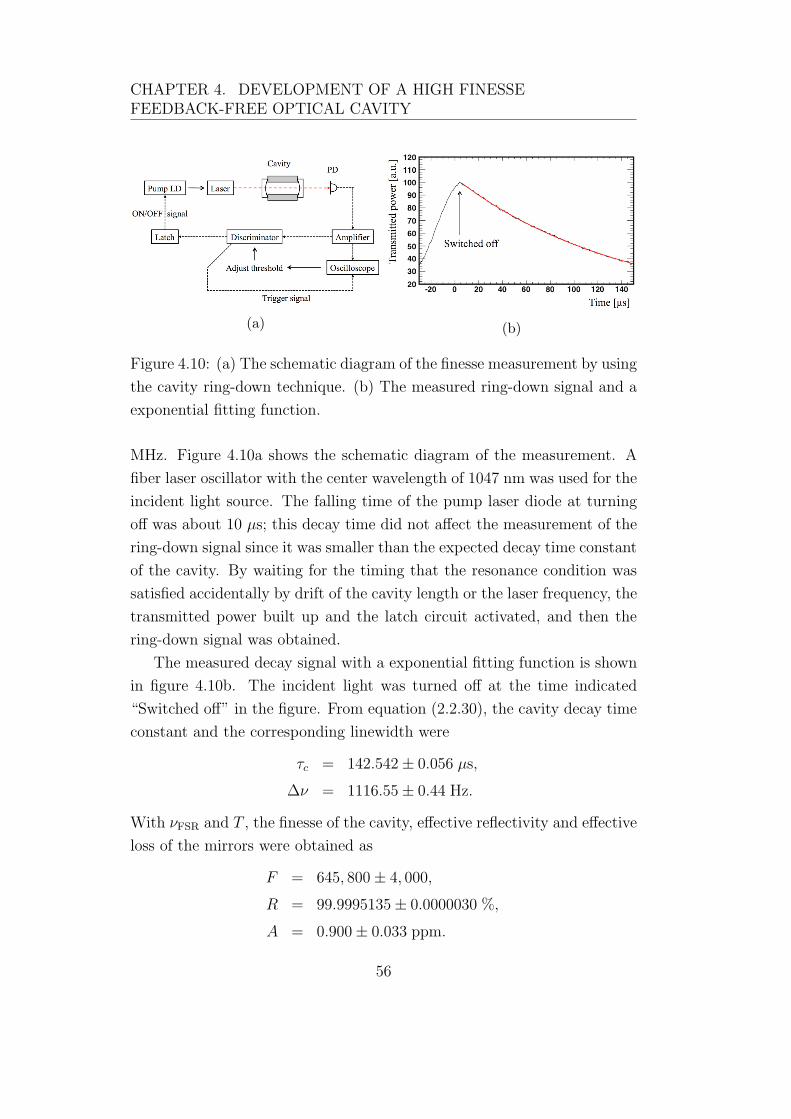
CHAPTER 4. DEVELOPMENT OF A HIGH FINESSEFEEDBACK-FREE OPTICAL CAVITY
(a) (b)
Figure 4.10: (a) The schematic diagram of the finesse measurement by using
the cavity ring-down technique. (b) The measured ring-down signal and a
exponential fitting function.
MHz. Figure 4.10a shows the schematic diagram of the measurement. A
fiber laser oscillator with the center wavelength of 1047 nm was used for the
incident light source. The falling time of the pump laser diode at turning
off was about 10 µs; this decay time did not affect the measurement of the
ring-down signal since it was smaller than the expected decay time constant
of the cavity. By waiting for the timing that the resonance condition was
satisfied accidentally by drift of the cavity length or the laser frequency, the
transmitted power built up and the latch circuit activated, and then the
ring-down signal was obtained.
The measured decay signal with a exponential fitting function is shown
in figure 4.10b. The incident light was turned off at the time indicated
“Switched off” in the figure. From equation (2.2.30), the cavity decay time
constant and the corresponding linewidth were
τc = 142.542± 0.056 µs,
∆ν = 1116.55± 0.44 Hz.
With νFSR and T , the finesse of the cavity, effective reflectivity and effective
loss of the mirrors were obtained as
F = 645, 800± 4, 000,
R = 99.9995135± 0.0000030 %,
A = 0.900± 0.033 ppm.
56

CHAPTER 4. DEVELOPMENT OF A HIGH FINESSEFEEDBACK-FREE OPTICAL CAVITY
These results were consistent with the ones expected by the mirror specifi-
cation.
4.2.2 Construction of a high finesse feedback-free op-
tical cavity
Figure 4.11: A schematic drawing of the optical setup of the feedback-free
cavity using the high finesse cavity. The detail is in main text.
Figure 4.12: A photograph of the cavity and optical components in the free-
space. The cavity consisted of a super-inver alloy tube and two ultra-low
loss mirrors.
Figure 4.11 shows a schematic drawing of the optical setup of the feedback-
free cavity with the high finesse cavity. The setup was almost same as the
57

CHAPTER 4. DEVELOPMENT OF A HIGH FINESSEFEEDBACK-FREE OPTICAL CAVITY
one for the low finesse case. An amplifier consisted of a single mod YDF
of the length of 38 cm and a pump LD. FI1 and 2 are Faraday isolators,
Coupler1 and 2 are fiber couplers to sent a part of circulating light to the
spectrum analyzer, and FC1 and 2 are the fiber collimator and coupler.
HWP and QWP1 are a half wave plate and a quarter wave plate to adjust
the polarization of light coming out from the fiber-space. PBS1 and 2 are
plate type polarized beamsplitters, whose transition and reflection ratio de-
pended on the wavelength as well as the angle of the devise with respect
to the optical axis and acted as low cut-off filters in the system. BPF is
an etalon-type band pass filter whose central wavelength was also able to
adjust. W1 and 2 are wedge plates to sample a part of intra-loop light to
monitor its power. QWP2 and 3 acted as additional optical isolators with
two PBSs. The high finesse cavity was aligned with the fundamental spatial
mode of the laser light coming from the fiber couplers by using matching
lens, L1 and 2.
Figure 4.12 is a photograph of the cavity and optical components on the
optical table. It should be noted that all components were set in the air
with room temperature, in acoustic shielding box.
Laser oscillation with the band pass filter
(a) (b)
Figure 4.13: (a) Observed laser powers as a function of the pump power. (b)
Observed power spectra averaged over 10 seconds. Each center wavelength
was chosen by the band pass filter.
58

CHAPTER 4. DEVELOPMENT OF A HIGH FINESSEFEEDBACK-FREE OPTICAL CAVITY
1046 nm 1047 nm 1048 nm 1049 nm
Threshold power Pth 240 mW 237 mW 220 mW 267 mW
Slop efficiency ηs 0.0117 0.0139 0.0178 0.0117
Table 4.1: Measured threshold powers and slope efficiencies in each chosen
wavelength condition.
Figure 4.14: Observed time variations of the laser powers around the cavity
for 100 seconds. The pump power was set 330 mW.
After adjusting optical components to reduce optical loss and select-
ing the laser wavelength around 1047 nm which is suitable for the gain of
the amplifier, the laser oscillation was observed. Figure 4.13a shows the ob-
served laser power sampled at PD3 as a function of the pump power. Linear
lines are fitting functions for each wavelength chosen by the band pass fil-
ter. The slopes of the functions and the thresholds of the laser oscillation
are summarized in table 4.1. Considering that the gain of the amplifier was
almost same in the wavelength range of a few nm, the difference between
obtained threshold powers can be attributed to the difference of the opti-
cal losses at each chosen wavelength. Furthermore, it is found that those
threshold powers were larger than ones of the low finesse case.
Figure 4.13b shows measured power spectra averaged over 10 seconds
59

CHAPTER 4. DEVELOPMENT OF A HIGH FINESSEFEEDBACK-FREE OPTICAL CAVITY
Figure 4.15: Observed power distributions at the wavelength of 1048 nm.
Black lines are fitting curves and dot lines indicate fitting ranges.
when the pump power was 330 mW. Each spectrum corresponds to the
wavelength chosen by the band pass filter. In a short time-period, each
spectrum had a narrower linewidth of less than 0.008 nm; it was determined
by the resolution of the spectrometer. And the center wavelength was
frequently fluctuating perhaps due to mode hopping, so the linewidth was
narrow, however, the lasing wavelength was not stable. Here, the lower limit
of the lasing wavelength was determined by the cut frequency of PBSs and
the upper limit was determined by the gain-bandwidth of the YDFA.
Figure 4.14 shows time variations of the laser powers around the cavity.
The data was for 100 seconds and the pump power was set 330 mW. The
incident, reflected and transmitted power measured by PD1, 2 and 3 were
corrected for the power sampling ratio of W1 and W2, respectively.
Observed power distributions at the wavelength of 1048 nm were shown
in figure 4.15, where the net input power Pnet was defined by subtracting
the reflected power Pre from the incident power Pin (Pnet = Pin − Pre).
Black lines are fit curves by Gaussian function. The fitting ranges were
chosen to avoid the tails of the distributions as indicated in figures. The
results of the laser power measurements are summarized in table 4.2.
60

CHAPTER 4. DEVELOPMENT OF A HIGH FINESSEFEEDBACK-FREE OPTICAL CAVITY
Light power [mW] 1046 nm 1047 nm 1048 nm 1049 nm
Incident Pin 5.694(2) 6.527(2) 8.794(2) 3.295(3)
Reflected Pre 3.195(1) 3.437(10) 4.159(1) 1.481(1)
Transmitted Ptr 1.069(1) 1.307(1) 1.961(1) 0.7938(8)
Net input P netin 2.497(2) 3.085(1) 4.633(2) 1.816(2)
Table 4.2: The results of the laser power measurements. Each value is
means values of the fit.
Laser oscillation without the band pass filter
(a) (b)
Figure 4.16: (a) Observed laser power at PD3 as a function of the pump
power in the case of no band pass filter. (b) Observed laser spectrum. The
spectrum shape was stable in long time unlike in the case of with the band
pass filter.
We also constructed the feedback-free cavity without the band pass
filter, and then laser oscillation successfully built up. Figure 4.16a shows
the observed laser power at PD3 as a function of the pump power. The red
line is the fitting line to the data. The threshold power was obtained as
181 mW and the slop efficiency was 0.0318 (in table 4.3b). It is found that
the threshold of the laser oscillation decreased comparing with the case of
laser oscillation with the band pass filter.
Figure 4.16b shows the observed laser spectrum. The center wavelength
was 1047 nm and the linewidth was 1.3 nm in FWHM. The shape of the
spectrum was stable in long time and its linewidth was wider than the one
61

CHAPTER 4. DEVELOPMENT OF A HIGH FINESSEFEEDBACK-FREE OPTICAL CAVITY
Figure 4.17: Observed time variation of the laser power around the cavity
for 100 seconds. The pump power was set 330 mW.
without BPF
Threshold power Pth 181 mW
Slop efficiency ηs 0.0318
(a)
Light power [mW] without BPF
Incident Pin 13.482(1)
Reflected Pre 2.556(1)
Transmitted Ptr 4.758(1)
Net input P netin 10.916(2)
(b)
Table 4.3: (a) Measured threshold power and slop efficiency in the case of
no band pass filter. (b) Measured intra-loop laser powers around the cavity.
for the spectra when the oscillation with the band pass filter. Figure 4.17
shows the time variation of the laser power around the cavity. The data
was for 100 seconds and the pump power was set 330 mW. It is found that
the laser power was stable and the coupling ratio (reflected power divided
by incident power) was better than the one of the results in the case of with
the band pass filter. Observed power distributions are shown in figure 4.18.
The data were fitted by Gaussian functions (black curves). All distributions
had widths of about 5 % in RMS, that was smaller than the widths of about
10 % in the case of with the band pass filter.
From the measurement results which are summarized in table 4.3b, we
think that the system laser oscillated as continuous multi mode operation;
the stable laser power, relativity large intensity noise and the especially wide
linewidth indicate it. When the band pass filter is inserted in the optical
loop, the build up of some longitudinal modes would be strongly suppressed.
62

CHAPTER 4. DEVELOPMENT OF A HIGH FINESSEFEEDBACK-FREE OPTICAL CAVITY
Figure 4.18: The measured power distributions without the band pass filter.
Black lines are Gaussian fitting functions.
In the case of with the band pass filter described above section, the laser
oscillation would have been forced to operate as single-mode-like (or in a
few number of longitude modes) by the filter, and actually such phenomena
was observed.
Robustness of the laser storage in multi mode operation
In generally, a single mode operated laser is weak against disturbance and
often mode-hops. On the other hand, a laser oscillator in multi mode
operation is great stable in its intensity. Therefore, it is expected that the
feedback-free cavity in multi mode operation (in the case of no band pass
filter) would also have good robustness.
Figure 4.19 shows the display of an oscilloscope which monitored the
laser power from PD3. Since the cavity was laser oscillating in multimode
operation, a certain constant optical power with some intensity noise was
observed. In order to understand its robustness, we hit the cavity body to
stop the laser oscillation. The dip signal in figure 4.19 indicates a moment
that the oscillation stopped, in other words, the resonant condition was
broken. However, the oscillation recovered automatically quickly as shown
63

CHAPTER 4. DEVELOPMENT OF A HIGH FINESSEFEEDBACK-FREE OPTICAL CAVITY
Figure 4.19: (a) The laser power was fell out at the impact, however, recov-
ered soon. (b) The recovery time of 40 ms was consistent with a damping
time of the mechanical vibration.
in figure 4.19 (b); the fall time was about 140 µs which was consistent with
the decay time constant of the cavity, and the recovery time of 40 ms was
consistent with a damping time of the mechanical vibration of the cavity
body. It is clearly evident the feedback-free cavity had the good stability
against external disturbances.
4.2.3 Evaluation of the system performance
The intra-cavity power Pcav and the power enhancement factor G were
evaluated. From the transmittance of the end mirror T2 and the measured
transmitted power Ptr, those were calculated as
Pcav = 2Ptr/T2, (4.2.1)
G = Pcav/Pin, (4.2.2)
where the transmittance was T2 = 3.77±0.02 ppm as introduced in previous
section. The results of the calculation are summarized in table 4.4. Errors
mainly resulted from the linearity uncertainty of the power meter of 0.5 %.
The stored laser power in the multi-mode oscillation was reached 2.52
kW by only 330 mW pump power. And the enhancement factor was also
reached more than 100,000 in all cases of operation. The observed enhance-
ment factor was, however, smaller than the expected ideal value Gid which
64

CHAPTER 4. DEVELOPMENT OF A HIGH FINESSEFEEDBACK-FREE OPTICAL CAVITY
Unit 1046 nm 1047 nm 1048 nm 1049 nm multi mode
Pcav [W] 567(3) 693(4) 1,040(6) 421(2) 2,524(13)
G [×103] 99.6(5) 106.2(6) 118.3(6) 127.8(7) 187.2(10)
Table 4.4: The results of the intra-cavity power and the power enhancement
factor. Each wavelength means the center wavelength chosen by the band
pass filter. The right side results indicates the case of no filter.
can be obtained by considering the ideal resonant condition as introduced
in chapter 2:
Gid =2T
(1−R)2∼ 2F
π= 411, 100± 2, 500. (4.2.3)
It should be noted that the optical loss at the cavity mirror was including
into this estimated ideal factor. The experimental result indicates that the
resonance state of the feedback-free cavity had certain phase difference from
the exact resonant condition.
4.3 Measurement of the frequency response
function
4.3.1 Measurement scheme and setup
We tried to measure the cavity finesse by using the frequency response
measuring technique (see section 3.3.3) while the cavity was laser oscillat-
ing with self-resonating mechanism in the multi mode operation. In order
to modulate the light intensity, we controlled the pump power driving the
YDFA. In general, the pump power modulation affects the population in-
version in the laser medium and causes chaotic behavior in the laser inten-
sity [41] because of the coupling term in two differential equations (2.3.10)
and (2.3.14). To avoid such instability, we had applied sufficiently small
modulation in the pump power (or population inversion). After tuning the
modulation depth by controlling the driving current to the LD, the mod-
ulation depth in the laser intensity was set at about 1 % with respect to
65

CHAPTER 4. DEVELOPMENT OF A HIGH FINESSEFEEDBACK-FREE OPTICAL CAVITY
Figure 4.20: A conceptual diagram of the pump power modulation scheme.
When the depth of the modulation is small enough, this scheme is same as
the intensity modulation technique described in section 3.3.3.
the steady-state laser intensity. Then we were able to treat transmutation
of the modulation signal as a liner equation of the photon density q as like
equation (2.3.25).
Figure 4.20 shows a conceptual diagram of the frequency response func-
tion measurement by using the pump power modulation method. The input
modulation signal u(Ω) of the pump rate r is applied to the closed loop sys-
tem of the photon density q via the transfer function of P (Ω), where the
modulation angular frequency Ω is sufficiently smaller than the free spec-
trum range of the cavity. x(Ω) and y(Ω) corresponds with the incident and
transmitted intensity of laser light. It should be noted that the light payed
attention here is not the total intensity but the sideband component; its op-
tical frequency would be ωc±Ω, where ωc is the center angular frequency of
the laser, and Ω is the modulation angular frequency. H(Ω) is the transfer
function of the cavity and A(Ω) is unknown transfer function. The transfer
function for x/u and y/u can be written as
x
u= P
A
1− AH, (4.3.1)
y
u= P
AH
1− AH. (4.3.2)
From these equations, we obtain
y
x=
PAH
PA= H. (4.3.3)
This relation shows that one can obtain the transfer function H(Ω) by
measuring the response functions of x(Ω) and y(Ω).
66

CHAPTER 4. DEVELOPMENT OF A HIGH FINESSEFEEDBACK-FREE OPTICAL CAVITY
Figure 4.21: A setup drawing of the response function measurement by
using the pump power modulation method.
Figure 4.21 shows the setup drawing of the response function measure-
ment. The feedback-free cavity was laser oscillating in multi mode operation
with pump power of 330 mW. The electrical current driving the pump LD
was modulated by using the sine wave signal generated from a function
generator (FG) with the modulation angular frequency of Ω. The modula-
tion bandwidth was up to 10 kHz (the bandwidth of LD was a few MHz).
The modulation depth was set to become 1 % at low frequency limit in the
laser power. The time variation of the incident power, Pin and the trans-
mitted power Ptr were measured by PDs with an oscilloscope. Observed
time variation of the PD signal was composed of the DC component and
the AC component; the DC corresponded with the steady-state light power
or carrier light power and the AC corresponded with sideband light power.
The AC signals of the incident and transmitted light gave the data sets of
the response of x(Ω) and y(Ω).
4.3.2 Result of the finesse measurement
Figure 4.22 shows the response function of y(f)/x(f). The red line is the
fitting function of a first-order low pass filter expressed as
|H(f)| = η0√1 + (f/fc)2
, (4.3.4)
67

CHAPTER 4. DEVELOPMENT OF A HIGH FINESSEFEEDBACK-FREE OPTICAL CAVITY
Figure 4.22: Obtained response function of y(f)/x(f). The red line is a
fitting function. The detail is in the main text.
where η0 and fc are fitting parameters. The cut-off frequency fc has the
relation with the resonance linewidth of the cavity:
∆ν = 2fc. (4.3.5)
From this linewidth, we can introduce the effective finesse, Feff , which in-
cludes performance of the self-resonating mechanism. The results of the
measurement and calculation are summarized as below:
η0 = 0.351± 0.002,
fc = 914± 23 Hz,
Feff = 394, 500± 10, 100.
The obtained effective finesse was smaller than the finesse obtained by using
the cavity ring-down technique in section 4.2.1.
4.4 Relaxation oscillations
In the case of the high finesse cavity, it is difficult to observe relaxation
oscillations in the time variation of the light intensity since the long cavity
decay time constant gives the damping ratio ζ close to 1. However, the
natural angular frequency ωn and more parameters in relaxation oscillations
can be measured by modulating photon density or laser intensity in the laser
68

CHAPTER 4. DEVELOPMENT OF A HIGH FINESSEFEEDBACK-FREE OPTICAL CAVITY
oscillator [42]. This frequency-domain measurement was just same as the
measurement described in before section; the desired response of the photon
density ∆q in equation (2.3.25) agrees with the obtained y(f) in figure 4.20.
Figure 4.23 shows the measured data set of y(f) as a function of the
modulation frequency. The red line is a fitting function of the second-order
low pass filter that is written as
F (f) =K
√√√√√
⎡
⎣1−(2πf
ωn
)2⎤
⎦2
+
[2ζ
(2πf
ωn
)]2, (4.4.1)
where K is a normalization factor. This fitting function corresponds with
the solution of the damping oscillation, equation (2.3.25). As a result of
the fit, the normalization factor K, the natural angular frequency ωn, and
the damping ratio ζ were obtained as
K = 399± 2,
ωn = 4.96± 0.08 kHz,
ζ = 0.586± 0.009.
With the experimental pump rate
r =330 mW
181 mW, (4.4.2)
and equation (2.3.26) and (2.3.27), the decay rates γ2 and γL were calculated
as
γ2 = 3.2 kHz,
γL = 9.4 kHz,
and the inverse of γ2 was
τ2 =1
γ2= 0.31 ms.
This obtained decay time constant τ2 is consistent with the magnitude of
the order of the typical fluorescence lifetime of the YDF (∼ 1 ms), however,
69

CHAPTER 4. DEVELOPMENT OF A HIGH FINESSEFEEDBACK-FREE OPTICAL CAVITY
Figure 4.23: Observed response of the transmitted sideband light power,
y(f) as a function of the modulation frequency. The red curve is a fitting
function of the second-order low pass filter.
it is shorter than the result in the case of low finesse (1.9 ms). The decay
rate of the laser cavity γL is expressed by equation (2.3.15),
γL =− lnαloop
τL. (4.4.3)
Assuming that the τL is same as the cavity decay time constant, τc ∼ 140
µs, which was the time constant measured by using the cavity ring-down
technique as described before section, the optical loss in the optical loop
αloop was estimated as −5.8 dB.
4.5 Discussion
The experimental results shows that the self-resonating mechanism is ca-
pable of very stable laser storage for high finesse cavities. The obtained
power enhancement factor achieved more than 100,000 and the storage op-
tical power was 2.5 kW with 330 mW pump power. The laser power had
relatively large intensity noise, however the mean of the lasing power was
quite stable. That stability was also shown in measurement results of re-
laxation oscillations (figure 4.23). The photon density in the feedback-free
cavity had vibration isolation against disturbance.
One of the questions to this system is why the cavity finesse was ob-
served to be small in the laser storage or laser oscillation. The finesse is
70

CHAPTER 4. DEVELOPMENT OF A HIGH FINESSEFEEDBACK-FREE OPTICAL CAVITY
originally defined only from the reflectance of the cavity mirror and gives
the enhancement factor of optical power or the interaction length in the
exact resonance condition. On the other hand, the effective finesse was in-
troduced from the enhancement factor of the interaction length, which has
a relation with the decay time constant of the transmitted light. In that
sense, the obtained finesse by using the cavity ring-down technique may
also be better to be called the effective finesse, however, there is difference
between the cavity ring-down technique and the frequency response func-
tion technique. In the later case, the laser light is continually irradiating the
cavity. The time variation of the phase difference in the resonance causes
the Doppler shift on the optical frequency of the intra-cavity light [43, 44].
Without the incident light, there is no effect on the intensity of the trans-
mitted light (ring-down signal), however, the presence of the incident light
field causes some intensity modulation caused by the interference between
the incident and transmitted light (see Appendix B).
In figure 4.21, the instantaneous frequency of the incident light would
have been different from the intra-cavity light since the incident light was
coherent light for the past light in the cavity. It can be presumed that the
inconsistency between the result of the cavity ring-down technique and the
result of the frequency response technique is caused by intensity modulation
due to the interference between incident light and transmitted light. We
could not analyze this matter in more detail in this experiment since the
laser oscillation in multi mode operation gives only the average intensity of
the light of a myriad of longitudinal modes. The same situation occurred
in the case of with the band pass filter since the central lasing wavelength
was frequently mode-hopping.
The result of relaxation oscillations is also measurement which gives in-
formation on the cavity finesse as the decay time constant of a laser cavity
τL. However, as we have seen, the measurement result showed that the
decay rate of the fluorescence γ2 was different from the fluorescence life-
time of a YDF and the result in the low finesse case. Since the fluorescence
lifetime is specific character of the atoms in a YDF, the value does not
change depending on the configuration of the optical setup. According to
reference [40], the YDF laser oscillator operating at the lasing wavelength
71

CHAPTER 4. DEVELOPMENT OF A HIGH FINESSEFEEDBACK-FREE OPTICAL CAVITY
of 1047 nm does not follow the strict four level system. For detailed veri-
fication, we will have to consider other models of relaxation oscillations in
quasi-three level systems. Furthermore, it will be necessary to improve the
experimental accuracy: change of the lasing wavelength, use of other cavity
finesses, use of different laser medium, etc.
72
Chapter 5
Conclusion
We successfully demonstrated the highly stable operation of a feedback-free
optical cavity with the self-resonating mechanism. In this work, the highly
stable operation with the effective finesse of 394, 000 ± 10, 000, which is
two orders of magnitude higher than our previous study [17], was achieved.
The stored power in the cavity was 2.52 ± 0.13 kW with stability of 1.7
% and the power enhancement factor of the cavity was 187, 000 ± 1, 000.
The results showed a scheme to overcome an issue to construct a high
finesse optical resonant cavity since required precision for the cavity length
to stabilize the cavity with this effective finesse and the power stability
is about 0.16 pm, which could only been achieved with a sophisticated
feedback control system. The system showed a continuous operation of
more than two hours with the power fluctuation of 1.7 %, showing high
robustness against environmental disturbances.
This study showed the possibility of realizing a high finesse cavity with-
out a sophisticated active feedback system. It is highly useful for applica-
tions, such as photon sources by laser Compton scattering, cavity enhanced
absorption spectroscopy (CEAS) [46–48] or the measurement of vacuum
magnetic birefringence [49, 50]. In later two applications, highly large en-
hancement of the optical interaction length is strongly required, however,
the narrow laser linewidth is not required. In particular, we can directly
apply the cavity ring-down technique or the response function technique to
the CEAS since it obtains information from the change of finesse by trace
73
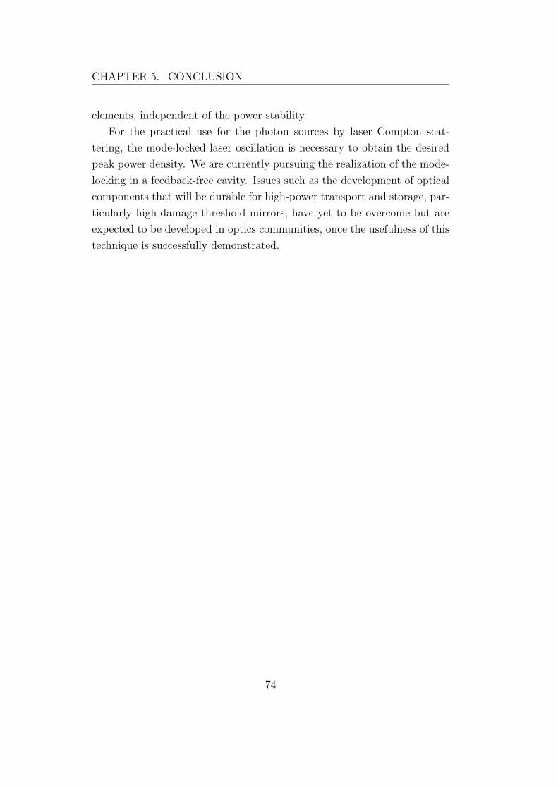
CHAPTER 5. CONCLUSION
elements, independent of the power stability.
For the practical use for the photon sources by laser Compton scat-
tering, the mode-locked laser oscillation is necessary to obtain the desired
peak power density. We are currently pursuing the realization of the mode-
locking in a feedback-free cavity. Issues such as the development of optical
components that will be durable for high-power transport and storage, par-
ticularly high-damage threshold mirrors, have yet to be overcome but are
expected to be developed in optics communities, once the usefulness of this
technique is successfully demonstrated.
74

Appendix A
A.1 Optical ray matrices
According to the Farmer’s law, light passes through arbitrary two positions
with minimum travel time as an optical ray. The ray is written by an optical
ray vector R with the transverse position r and the divergence angle r′ with
regard to an optical axis:
R =
(r
r′
). (A.1.1)
Consider an incident ray vector Rin enters an optical system and the cor-
responding output ray vector Rout exits the system, the optical system can
be expressed by a 2× 2 matrix:
Rout =
(A B
C D
)Rin, (A.1.2)
where A,B,C,D are matrix elements. This matrix is called as the ray
matrix and its matrix elements depends on each optical component; for
free propagation of distance d, the ray matrix is given by
D =
(1 d
0 1
); (A.1.3)
for focus or defocus the rays by using a lens with a focal length of f , the
ray matrix is given by
F =
(1 0
−1/f 1
). (A.1.4)
75
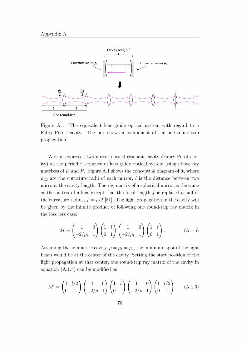
Appendix A
Figure A.1: The equivalent lens guide optical system with regard to a
Fabry-Perot cavity. The box shows a component of the one round-trip
propagation.
We can express a two-mirror optical resonant cavity (Fabry-Perot cav-
ity) as the periodic sequence of lens guide optical system using above ray
matrixes of D and F . Figure A.1 shows the conceptual diagram of it, where
ρ1,2 are the curvature radii of each mirror, l is the distance between two
mirrors, the cavity length. The ray matrix of a spherical mirror is the same
as the matrix of a lens except that the focal length f is replaced a half of
the curvature radius, f = ρ/2 [51]. The light propagation in the cavity will
be given by the infinite product of following one round-trip ray matrix in
the loss less case:
M =
(1 0
−2/ρ2 1
)(1 l
0 1
)(1 0
−2/ρ1 1
)(1 l
0 1
). (A.1.5)
Assuming the symmetric cavity, ρ = ρ1 = ρ2, the minimum spot of the light
beam would be at the center of the cavity. Setting the start position of the
light propagation at that center, one round-trip ray matrix of the cavity in
equation (A.1.5) can be modified as
M ′ =
(1 l/2
0 1
)(1 0
−2/ρ 1
)(1 l
0 1
)(1 0
−2/ρ 1
)(1 l/2
0 1
). (A.1.6)
76

Appendix A
A.2 Gaussian beams
By paraxial approximating the wave equation of electromagnetic waves
around the z axis, which is the optical axis, we obtain the two-dimensional
Schrodinger equation as follows:
∂2u
∂x2+
∂2u
∂y2+ 2ik
∂u
∂z= 0, (A.2.1)
where u is the amplitude of the light field; k = 2π/λ is the wave number of
light, where λ is the wavelength of light. This equation has set of solutions
which is generally called as high-order Gaussian modes; Hermite-Gaussian
modes, Laguerre-Gaussian Modes, and so on [51,52].
Characteristic of the lowest or fundamental mode of solutions of equa-
tion (A.2.1) is the most important to describe the propagation of the parax-
ial optical wave since high-order modes can be derived from the fundamen-
tal mode by utilizing the ladder operator in operator methods [53]. The
normalized form of the fundamental mode is given by [51]
u(r, z) =w0
w(z)exp
−i[kz − η(z)]− r2
w2(z)+ i
kr2
2R(z)
, (A.2.2)
where
η(z) = tan−1
(λz
πw0
)(A.2.3)
is the Guoy phase, w(z) is the radius size where the light field amplitude
becomes 1/e from the optical axis, w0 is its minimum value chosen at z = 0,
and R(z) is the curvature radius of the wavefront of the light beam. w(z)
and R(z) are functions of λ and w0 defined as follows:
w(z) = w0
√
1 +
(λz
πw20
)2
, (A.2.4)
R(z) = z
[1 +
(πw2
0
λz
)2]. (A.2.5)
The light propagation formed by the fundamental mode, the Gaussian
beam, obeys these functions as shown in figure A.2. The position where the
radius size becomes the minimum w0 is called the beam waist. At the waist,
77

Appendix A
Figure A.2: Propagation of the Gaussian beam. An origin of the propaga-
tion direction z is set to the waist position.
the Gaussian beam has infinite wavefront curvature that is a flat wavefront.
Furthermore, at positions far enough apart from Rayleigh range, which is
defined as
zR =πw2
0
λ, (A.2.6)
the light beam becomes equal to the spherical wave emitted from the point
light source. The divergence angle θ of the beam is given by
tan θ ∼ θ =λ
πw0, (A.2.7)
where approximation of tan holds when θ is sufficiently small.
A.3 Gaussian beam in a Fabry-Perot cavity
The propagation of the Gaussian beam can track using a ray matrix as well
as geometric rays. The complex beam parameter, q(z), consisting of w(z)
and R(z) is introduced as follows:
1
q(z)=
1
R(z)+
2i
kw2(z). (A.3.1)
The beam parameter at the waist (z = 0) is given by
q(0) = − iπw20
λ. (A.3.2)
Before and after the Gaussian beam passes through optical system, the
beam parameters change as follows [51]:
qout =qinA+B
qinC +D, (A.3.3)
78

Appendix A
Figure A.3: Plots of the minimum focal spot size w0 as a function of the
curvature radius ρ with the fixed cavity length (left side) and a function of
the the cavity length l with the fixed curvature radius (right side).
where qin,out are beam parameters of the incident and output beam, and
A,B,C,D are matrix elements of this system.
Let’s consider the propagation of the Gaussian beam in a symmetric
Fabry-Perot cavity. The stable Gaussian mode of the cavity is obtained
from following self-consistent relation:
q =Aq +B
Cq +D. (A.3.4)
Taking into account the the condition on the determinant, AD − BC = 1,
solution of this equation for 1/q is
1
q=
D − A
2B± i
√4− (D + A)2
2B. (A.3.5)
Thus, mode shape on reference plane is obtained as
R =2B
D − A, (A.3.6)
w2 =2λ|B|
π√4− (D + A)2
. (A.3.7)
Substituting the one round-trip matrix (A.1.6) into equation (A.3.7), we
obtain the minimum focal spot size of the Gaussian beam in the symmetric
Fabry-Perot cavity. (Note that the wavefront is flat since it is the waist of
79

Appendix A
the Gaussian beam.) Figure A.3 shows the the minimum focal spot size w0
as a function of the curvature radius ρ with the fixed cavity length (left side)
and a function of the the cavity length l with the fixed curvature radius
(right side). Here, the wavelength of light, curvature radius and cavity
length are chosen 1047 nm, 0.5 m and 0.208 m, respectively. It is found
that the spot size can be reduced by bringing the cavity length closer to
twice of the curvature radius, however, the cavity cannot confine the light
when the curvature radius is smaller than a half of the cavity length. Hence,
the achievable focusing size will be limited by the geometric accuracy of the
cavity.
80

Appendix B
B.1 Dynamic characteristics of a Fabry-Perot
cavity
Consider a Fabry-Perot cavity composed of two mirrors, and its light fields
as shown in figure B.1. Suppose a is the position of the input mirror surface
and b is the position of the end mirror surface, and b changes over time with
respect to a; the position of b from an origin x = 0 is x = x′(t). L is the
initial cavity length which is larger than the variation x′(t)− L of the end
mirror. The time interval required for the light to make one round-trip in
the cavity is given by
T =2L
c. (B.1.1)
Let the light entering the cavity be a continuous monochromatic plane
wave with the frequency of ω and the amplitude of Ein. Here, the initial
Figure B.1: A Fabry-Perot cavity and its light field. The position of the
end mirror b changes over time with respect to a.
81

Appendix B
cavity length L is an integral multiple of the wavelength of the incident
light and it satisfies the following resonance condition:
exp (−iωT ) = exp (−2ikL) = 1, (B.1.2)
where k = ω/c is the wave number, and c is the speed of light. The
forward electric field Ef and the backward electric field Eb within the cavity
immediately after the input mirror surface a are given by [43]
Eb(t) = −rbEf (t− T ) exp [−2ikx(t− T/2)], (B.1.3)
Ef (t) = taEin − raEb(t), (B.1.4)
where ra, rb are reflection coefficients of the input (a) and end (b) mirrors,
and ta, tb are transmission coefficients of those; x(t) is the variation of b
from the initial cavity length L:
x(t) = x′(t)− L. (B.1.5)
The exponential part on the right side of equation (B.1.3) represents the
phase change given by the end mirror after the intra-cavity light travels one
round-trip in the cavity. Summarizing two equations (B.1.4) and (B.1.4),
we obtained the expression for Ef as
Ef (t) = taEin + rarbEf (t− T ) exp [−2ikx(t− T/2)], (B.1.6)
and the expression for Eb as
Eb(t) = [−tarbEin + rarbEb(t− T )] exp [−2ikx(t− T/2)]. (B.1.7)
Differential equations of intra-cavity fields
Assuming that the velocity of the end mirror surface b is constant v:
x(t) = vt. (B.1.8)
When the finesse is sufficiently high, the magnitude of the electric field
inside the cavity does not change significantly in the interval T . Thus, we
82

Appendix B
can treat the interval T as a fraction of time, dt, and we can obtain the
differential equation of Ef as follows [43]:
dEf (t)
dt∼ Ef (t+ T )− Ef (t)
T
=taEin
T+ (rarb exp [−2ikv(t+ T/2)]− 1)
Ef (t)
T. (B.1.9)
Since the change in position of the mirror surface b while going through the
cavity’s resonance point is sufficiently smaller than the cavity length L, the
phase change of the electric field given by b can be approximated as follows:
exp [−2ikvt] ∼ 1− 2ikvt. (B.1.10)
Substituting this in equation (B.1.9) and eliminating the phase offset, we
obtain the following linear differential equation:
dEf (t)
dt∼ taEin
T+
[rarb − 1
T− 2irarbkv
Tt
]Ef (t). (B.1.11)
Similarly for Eb, we obtain
dEb(t)
dt∼ −tarbEin
Texp [−2ikv(t+ T/2)]
+ (rarb exp [−2ikv(t+ T/2)]− 1)Eb(t)
T
∼ −tarbEin
T+
2itarbkv
TEint
+
[rarb − 1
T− 2irarbkv
Tt
]Eb(t). (B.1.12)
Calculation examples
The transmitted field Etr and reflected field Ere from the cavity are given
by
Etr(t) = tbEf (t− T/2), (B.1.13)
Ere(t) = raEin + taEb(t). (B.1.14)
Figure B.2 and figure B.3 show plots of the transmitted and reflected light
intensities ,I(t) = E(t)E∗(t), calculated with several values of v, where the
83
Appendix B
Figure B.2: Red line: transmitted light intensity, blue line: return light
intensity. Only one response peak is observed when the mirror speed is
slow.
Figure B.3: Red line: transmitted light intensity, blue line: return light
intensity. The scales on the horizontal axis are same. Peaks are tilted and
the ringing appears at foots of the peaks.
initial cavity length is L = 1.68 m, the wavelength is λ = 1064 nm, the
reflectivity of the cavity mirrors is R = 0.9999, and the transmittance is
T = 1−R; the incident amplitude is set to Ein = 1.
With the small mirror velocity v, the intensities behave like figure 2.7
and figure 2.8 (see figure B.2). As the velocity gets bigger, the peak is tilted
and the ringing starts to appear at the foot of the peak (see figure B.3).
Furthermore, it is found that the peak intensity in the transmitted light
decreases, and the peak intensity in the reflected light is larger than the
incident light intensity.
B.2 Finesse measurement by ringing effects
When the cavity length of a Fabry-Perot cavity is swept with slow change
rate, the symmetrical resonant peaks of the intensity of transmitted light as
84

Appendix B
Figure B.4: A result of the finesse measurement with the ringing effect
technique. The detail is in the main text.
shown in figure 2.7 are observed. However, when the velocity of the change
is quick, the transmitted light exhibits different behavior, depending on the
velocity of the mirror, the cavity finesse and the free spectral range of the
cavity as shown in the previous section. This phenomenon is understood
based on the Doppler effect of the optical frequency in the cavity. The
ringing effect can be employed as an application to measure the cavity
finesse [54]. In this method, the ratio between the first peak power and
the second peak power of the ringing and the time interval ∆t between
two peaks are measured. Then the finesse is obtained as the value of the
variable πc∆t/l at the ratio being e = 2.71 · · · , where c is the speed of light,
l is the cavity length.
With this ringing effect technique, we measured the finesse of a Fabry-
Perot cavity which consisted of two ultra-low loss mirrors provided by LMA;
those mirrors had the reflectivity of about 99.999 % according to the spec-
ification; the expected finesse and the linewidth were about 300,000 and a
few kHz. In the original technique in [54], the ringings were produced by
sweeping the cavity length by a piezo-electric actuator with various veloc-
ity. In our case, the mirror position was always disturbed by some small
mechanical noise due to the narrow linewidth of the cavity and the peaks
always had the ringings. We were not able to control the velocity of the
85
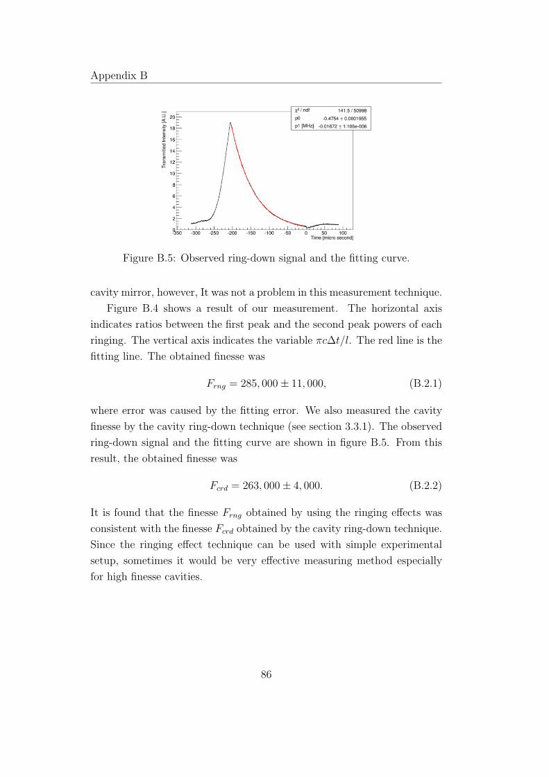
Appendix B
Figure B.5: Observed ring-down signal and the fitting curve.
cavity mirror, however, It was not a problem in this measurement technique.
Figure B.4 shows a result of our measurement. The horizontal axis
indicates ratios between the first peak and the second peak powers of each
ringing. The vertical axis indicates the variable πc∆t/l. The red line is the
fitting line. The obtained finesse was
Frng = 285, 000± 11, 000, (B.2.1)
where error was caused by the fitting error. We also measured the cavity
finesse by the cavity ring-down technique (see section 3.3.1). The observed
ring-down signal and the fitting curve are shown in figure B.5. From this
result, the obtained finesse was
Fcrd = 263, 000± 4, 000. (B.2.2)
It is found that the finesse Frng obtained by using the ringing effects was
consistent with the finesse Fcrd obtained by the cavity ring-down technique.
Since the ringing effect technique can be used with simple experimental
setup, sometimes it would be very effective measuring method especially
for high finesse cavities.
86

Bibliography
[1] W.J. Brown, F.V. Hartemann, “Three-dimensional time and frequency-
domain theory of femtosecond x-ray pulse generation through Thomson
scattering”, Phys. Rev. ST Accel. Beams 7 (2004) 060703.
[2] K. Sakaue et al., “Observation of pulsed x-ray trains produced by laser-
electron Compton scatterings”, Rev. Sci. Intrum. 80 (12) (2009) 123304.
[3] C. Sun, Y.K. Wu, “Theoretical and simulation studies of characteristics
of a Compton light source”, Phys. Rev. ST Accel. Beams 14 (2011)
044701.
[4] V. Petrillo et al., “Photon flux and spectrum of γ-rays Compton
sources”, Nucl. Instrum. Methods Phys. Res. A 693 (2012) 109.
[5] T. Okugi et al., “Proposed Method to Produce a Highly Polarized e+
Beam for Future Linear Colliders”, Jpn. J. Appl. Phys. 35, 3677 (1996).
[6] T. Omori et al.,“Efficient Propagation of Polarization from Laser Pho-
tons to Positrons through Compton Scattering and Electron-Positron
Pair Creation”, Phys. Rev. Lett. 96 (2006) 114801.
[7] L. Karim, “Measurement of the positron polarization at an helical
undulator based positron source for the International Linear Col-
lider ILC”, PhD, Humboldt-Universitat zu Berlin, Mathematisch-
Naturwissenschaftliche Fakultat I (2009).
[8] T. Behnke, J. E. Brau, B. Foster, J. Fuster, M. Harrison, J. M. Paterson,
M. Peskin, M. Stanitzki, N. Walker, H. Yamamoto, (Editors), “THE
87

Bibliography
INTERNATIONAL LINEAR COLLIDER Technical Design Report -
Volume 1: Executive Summary”, www.linearcollider.org
[9] H. Baer, T. Barklow, K. Fujii, Y. Gao, A. Hoang, S. Kanemura, J. List,
H. E. Logan, A. Nomerotski, M. Perelstein, M. E. Peskin, R. Poschl, J.
Reuter, S. Riemann, A. Savoy-Navarro, G. Servant, T. M. P. Tait, J. Yu,
(Editors), “THE INTERNATIONAL LINEAR COLLIDER Technical
Design Report - Volume 2: Physics”, www.linearcollider.org
[10] C. Adolphsen, et al., (Editors), “THE INTERNATIONAL LINEAR
COLLIDER Technical Design Report Volume 3.i: Accelerator R&D”,
www.linearcollider.org
[11] C. Adolphsen, et al., (Editors), “THE INTERNATIONAL LINEAR
COLLIDER Technical Design Report Volume 3.ii: Accelerator Baseline
Design”, www.linearcollider.org
[12] T. Behnke, J. E. Brau, P. Burrows, J. Fuster, M. Peskin, M. Stanitzki,
Y. Sugimoto, S. Yamada, H. Yamamoto, (Editors), “THE INTERNA-
TIONAL LINEAR COLLIDER Technical Design Report Volume 4: De-
tectors”, www.linearcollider.org
[13] For example, Z. Huang and R. D. Ruth, “Laser-Electron Storage
Ring”, submitted to Phys. Rev. Lett., SLAC-PUB-7556 (1997).
[14] H. Shimizu, S. Araki, Y. Funahashi, Y. Honda, T. Okugi, T. Omori,
N. Terunuma, J. Urakawa, M. Kuriki, S. Miyoshi, T. Takahashi, Y.
Ushio, T. Hirose, K. Sakaue, M. Washio, P. Guoxi and X. Li, “Photon
Generation by Laser-Compton Scattering Using an Optical Resonant
Cavity at the KEK-ATF Electron Ring”, JPSJ, 78, 7, 074501 (2009).
[15] S. Miyoshi, T Akagi, S. Araki, Y. Funahashi, T. Hirose, Y. Honda,
M. Kuriki, X. Li, T. Okugi, T. Omori, G. Pei, K. Sakaue, H. Shimizu,
T. Takahashi, N. Terunuma, J. Urakawa, Y. Ushio and M. Washio,
“Photon generation by laser-Compton scattering at the KEK-ATF”,
Nucl. Instr. Meth. A 623, 576-578 (2010).
88

Bibliography
[16] T. Akagie, et al., “Production of gamma rays by pulsed laser beam
Compton scattering off GeV-electrons using a non-planar four-mirror
optical cavity”, J. of Instr. 7, 001021 (2012).
[17] T. Akagi, S. Araki, Y. Funahashi, Y. Honda, H. Kataoka, T. Kon, S.
Miyoshi, T. Okugi, T. Omori, K. Sakaue, H. Shimizu, T. Takahashi,
R. Tanaka, N. Terunuma, J. Urakawa, M. Washio, H. Yoshitama, “De-
velopment of a three dimensional four mirror optical cavity for laser-
Compton scattering”, Nucl. Instr. Meth. A 724, 63 (2013).
[18] T. Akagi, S. Araki, Y. Funahashi, Y. Honda, S. Miyoshi, T. Okugi, T.
Omori, H. Shimizu, K. Sakaue, T. Takahashi, R. Tanaka, N. Terunuma,
Y. Uesugi, J. Urakawa, M. Washio, and H. Yoshitama, “Demonstration
of the Stabilization Technique for Nonplanar Optical Resonant Cavities
Utilizing Polarization”, Rev. Sci. Instr. 86, 043303 (2015).
[19] A. Borzsonyi, R. Chiche, E. Cormier, R. Flaminio, P. Jojart, C. Michel,
K. Osvay, L. Pinard, V. Soskov, A. Variola, and F. Zomer, “External
cavity enhancement of picosecond pulses with 28,000 cavity finesse”,
Appl. Opt., 52, 34 (2013).
[20] Y. Honda, H. Shimizu, K. Sakaue, J. Urakawa, N. Sasao and T. Omori,
“Photon Target using Self-start Build-up Cavity for Laser Compton
Sources”, Proc. 7th Annual Meeting of PASJ, 1102 (2010), in Japanese.
[21] G. T. Harvey and L. F. Mollenauer, “Harmonically mode-locked fiber
ring laser with an internal Fabry-Perot stabilizer for soliton transmis-
sion”, Opt. Lett., 18, 2 (1993).
[22] X. P. Cheng, P. Shum, C. H. Tse, J. L. Zhou, M. Tang, W. C. Tan, R.
F. Wu and J. Zhang, “Single-Longitudinal-Mode Erbium-Doped Fiber
Ring Laser Based on High Finesse Fiber Bragg Grating Fabrv-Perot
Etalon”, IEEE Phot. Tech. Lett., 20, 12 (2008).
[23] S. H. Parka, V. N. Litvinenkob, W. Tornowc, C. Montgomery, “Spatial
distribution and polarization of γ-rays generated via Compton backscat-
tering in the Duke/OK-4 storage ring FEL”, Nuc. Inst. Meth. A 475
(2001) 425-431.
89

Bibliography
[24] W. J. Brown and F. V. Hartemann, “Three-dimensional time and
frequency-domain theory of femtosecond x-ray pulse generation through
Thomson scattering”, Phys. Rev. ST Accel. Beams 7, 060703 (2004).
[25] C. Sun and Y. K. Wu, “Theoretical and simulation studies of charac-
teristics of a Compton light source”, Phys. Rev. ST Accel. Beams 14,
044701 (2011).
[26] V. Petrillo, et al., “Photon flux and spectrum of g-rays Compton
sources”, Nuc. Inst. Meth. A 693 (2012) 109-116.
[27] V. B. Berestetskii, L. P. Pitaevskii, E. M. Lifshitz, “Quantum Electro-
dynamics, Second Edition: Volume 4”, Butterworth-Heinemann, Lon-
don (1982).
[28] P. R. Saulson, “Fundamentals of Interferometric Gravitational Wave
Detectors”, chapter 6, World Scientific Pub. Co. Inc. (1994).
[29] A. Yariv and P. Yeh, “Photonics, Optical Electronics in Modern Com-
munication, Sixth edition”, Oxford University Press, Inc. (2006) pp. 212
Japanese edition.
[30] M. Rakhmanov, “Doppler-induced dynamics of fields in Fabry-Perot
cavities with suspended mirrors”, Appl. Opt., 40, 12 (2001).
[31] M. Rakhmanov, R. L. Savage Jr., D. H. Reitze, D. B. Tanner, ”Dy-
namic resonance of light in Fabry-Perot cavities”, Phys. Rev. Lett. A
305, 239-244 (2002).
[32] A. Yariv and P. Yeh, “Photonics, Optical Electronics in Modern Com-
munication, Sixth edition”, Oxford University Press, Inc. (2006) pp. 297
Japanese edition.
[33] M. Gorjan, T. North and Martin Rochette, “Model of the amplified
spontaneous emission generation in thulium-doped silica fibers”, J. Opt.
Soc. Am. B 29, 10 (2012).
[34] R. Paschotta, J. Nilsson, A. C. Tropper and D. C. Hanna, “Ytterbium-
Doped Fiber Amplifiers”, IEEE J. of Quant. Electro., 33, 7 (1997).
90

Bibliography
[35] A. E. Siegman, ”Lasers”, University Science Books, Mill Valley, Cali-
fornia, USA (1986) pp. 954-969.
[36] For example, K. Etoh, K. Sekine, M. Watanabe, K. Ito and K. Watan-
abe, “Development of ultra low loss mirrors for high finesse cavity”,
Japan Aviation Electronics Industry, Ltd., 航空電子技報 No.36 (2014),
in Japanese.
[37] D. Tatsumi, A. Ueda, “Development of the Ultra-Low Loss Mirrors
for Gravitational Wave Detector”, Annualr report of the national as-
tronomical observatory of Japan (ISSN 1346-1192), Vol. 14, 2011, pp.
21.
[38] M. Phelps, L. Zhang, R. Dannenburg, “Drag Wiping with Methanol
vs First Contact”, LIGO-T1000137 v3 (2010), www.ligo.caltech.edu
[39] N. Uehara and K. Ueda, “Accurate measurement of ultralow loss in
a high-finesse Fabry-Perot interferometer using the frequency response
functions”, Appl. Phys. B 61, 9-15 (1995).
[40] L. Orsila and O. G. Okhotnikov, “Three- and four-level transition dy-
namics in Ybfiber laser”, Opt. Exp. 13, 9, 3219 (2005).
[41] A. N. Pisarchik, A. V. Kir ’yanov and Y. O. Barmenkov, “Dynam-
ics of an erbium-doped fiber laser with pump modulation: theory and
experiment”, Opt. Soc. Am. B, 22, 10, 2811 (2005).
[42] A. E. Siegman, ”Lasers”, University Science Books, Mill Valley, Cali-
fornia, USA (1986) pp. 971-973.
[43] M. J. Lawrence, B. Willke, M. E. Husman, E. K. Gustafson and R. L.
Byer, “ Dynamic response of a Fabry-Perot interferometer”, Opt. Soc.
Am. B 16, 4 ,523 (1999).
[44] M. Rakhmanov, “Doppler-induced dynamics of fields in Fabry-Perot
cavities with suspended mirrors”, App. Opt. 40, 12 , 1942(2001).
91
Bibliography
[45] H. Carstens, N. Lilienfein, S. Holzberger, C. Jocher, T. Eidam, J.
Limpert, A. Tunnermann, J. Weitenberg, D. C. Yost, A. Alghamdi,
Z. Alahmed, A. Azzeer, A. Apolonski, E. Fill, F. Krausz, I. Pupeza,
“Megawatt-scale average-power ultrashort pulses in an enhancement
cavity”, Opt. Lett., 39, 9, 2595 (2014).
[46] A. O’Keefe and D. A. G. Deacon, “Cavity ring-down optical spectrom-
eter for absorption measurements using pulsed laser sources”, Rev. Sci.
Inst., 59, 2544 (1988).
[47] G. Gagliardi, H. P. Loock eds, “Cavity-Enhanced Spectroscopy and
Sensing” Springer Series in Optical Sciences (2014), ISBN: 978-3-642-
40002-5.
[48] K. Stelmaszczyk, P. Rohwetter, M. Fechner, M. Queiβer, A.
CzySewski, T. Stacewicz, and L. Woste, “Cavity Ring-Down Absorp-
tion Spectrography based on filament-generated supercontinuum light”,
Opt. Exp., 17, 5, 3673 (2009).
[49] F. Della Valle, E. Milotti, A. Ejlli, G. Messineo, L. Piemontese, G.
Zavattini, U. Gastaldi, R. Pengo and G. Ruoso, “First results from
the new PVLAS apparatus: A new limit on vacuum magnetic birefrin-
gence”, Phys. Rev. D,s 90, 092003 (2014).
[50] A. Cadene, P. Berceau, M. Fouche, R. Battesti and C. Rizzoa, “Vac-
uum magnetic linear birefringence using pulsed fields: status of the
BMV experiment”, Eur. Phys. J. D (2014) 68: 16.
[51] H. Kogelkin and T. li, “Laser beam and resonator”, Appl. Opt. 5, 10
(1966).
[52] A. E. Siegman, ”Lasers”, University Science Books, Mill Valley, Cali-
fornia, USA (1986) pp. 642-652.
[53] G. Nienhuis and L. Allen, “Paraxial wave optics and harmonic oscilla-
tors”, Phys. Rev. A 48, 1 (1993).
92

Bibliography
[54] J. Poirson, F. Bretenaker, M. Vallet and A. L. Floch, “Analytical and
experimental study of ringing effects in a Fabry-Perot cavity. Appli-
cation to the measurement of high finesses”, Opt. Soc. Am. B 14, 11
(1997) pp. 2811-2817.
93

公表論文
(1) Feedback-free optical cavity with self-resonating mechanism Y. Uesugi, Y. Hosaka, Y. Honda, A. Kosuge, K. Sakaue, T. Omori, T. Takahashi, J. Urakawa and M. Washio APL Photonics 1, 026103-1-7 (2016); doi: 10.1063/1.4945353

参考論文
(1) Demonstration of the Stabilization Technique for Nonplanar Optical Resonant Cavities Utilizing Polarization T. Akagi, S. Araki, Y. Funahashi, Y. Honda, S. Miyoshi, T. Okugi, T. Omori, H. Shimizu, K. Sakaue, T. Takahashi, R. Tanaka, N. Terunuma, Y. Uesugi, J. Urakawa, M. Washio and H. Yoshitama Review of Scientific Instruments 86, 043303-1-7 (2015); doi: 10.1063/1.4918653
(2) Development of an intense positron source using a crystal-amorphous hybrid target for linear colliders Y. Uesugi, T. Akagi, R. Chehab, O. Dadoun, K. Furukawa, T. Kamitani, S. Kawada, T. Omori, T. Takahashi, K. Umemori, J. Urakawa, M. Satoh, V. Strakhovenko, T. Suwada and A. Variola Nuclear Instruments and Methods in Physics Research B, 319, 17-23 (2014); doi:10.1016/j.nimb.2013.10.025