Delta Hedge - 國立臺灣大學lyuu/finance1/2007/20070509.pdf · Delta Hedge (concluded) †...

Delta Hedge

• The delta (hedge ratio) of a derivative f is defined as∆ ≡ ∂f/∂S.

• Thus ∆f ≈ ∆×∆S for relatively small changes in thestock price, ∆S.

• A delta-neutral portfolio is hedged in the sense that it isimmunized against small changes in the stock price.

• A trading strategy that dynamically maintains adelta-neutral portfolio is called delta hedge.

c©2007 Prof. Yuh-Dauh Lyuu, National Taiwan University Page 500

Delta Hedge (concluded)

• Delta changes with the stock price.

• A delta hedge needs to be rebalanced periodically inorder to maintain delta neutrality.

• In the limit where the portfolio is adjusted continuously,perfect hedge is achieved and the strategy becomesself-financing.

• This was the gist of the Black-Scholes-Merton argument.


Implementing Delta Hedge

• We want to hedge N short derivatives.

• Assume the stock pays no dividends.

• The delta-neutral portfolio maintains N ×∆ shares ofstock plus B borrowed dollars such that

−N × f + N ×∆× S −B = 0.

• At next rebalancing point when the delta is ∆′, buyN × (∆′ −∆) shares to maintain N ×∆′ shares with atotal borrowing of B′ = N ×∆′ × S′ −N × f ′.

• Delta hedge is the discrete-time analog of thecontinuous-time limit and will rarely be self-financing.


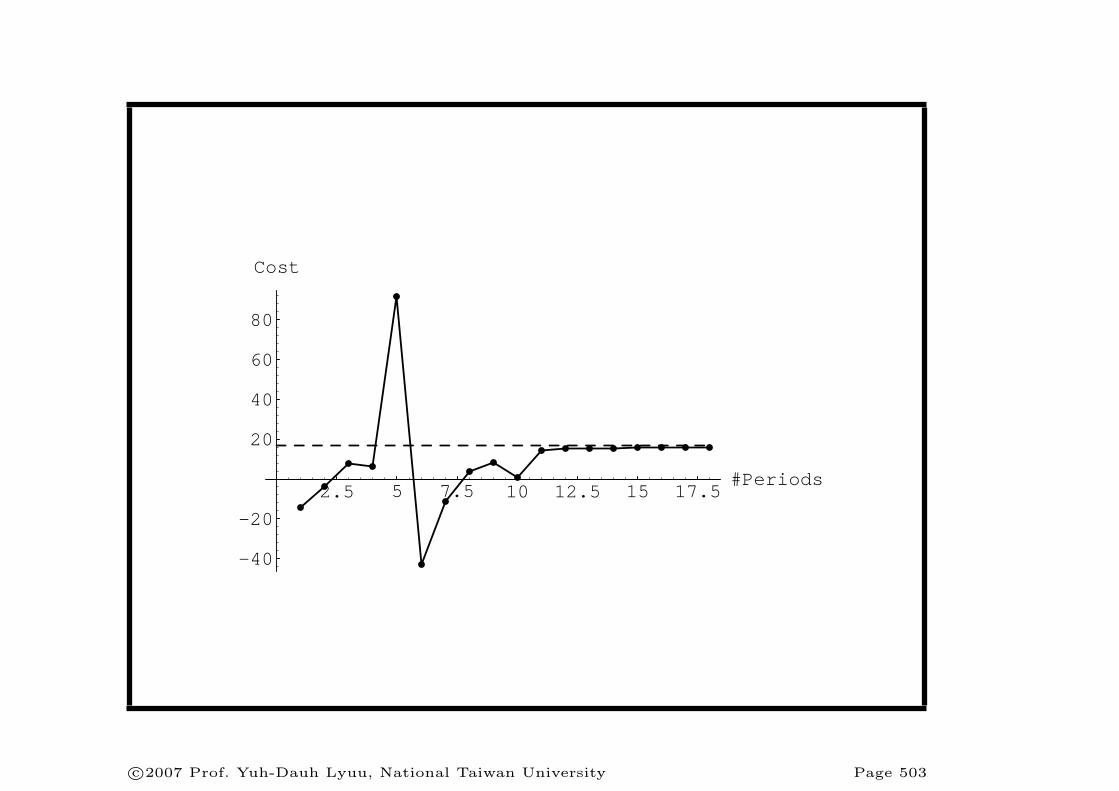
2.5 5 7.5 10 12.5 15 17.5#Periods

-40

-20

20

40

60

80

Cost


Example

• A hedger is short 10,000 European calls.

• σ = 30% and r = 6%.

• This call’s expiration is four weeks away, its strike priceis $50, and each call has a current value of f = 1.76791.

• As an option covers 100 shares of stock, N = 1,000,000.

• The trader adjusts the portfolio weekly.

• The calls are replicateda well if the cumulative cost oftrading stock is close to the call premium’s FV.

aThis example takes the replication viewpoint.

c©2007 Prof. Yuh-Dauh Lyuu, National Taiwan University 04

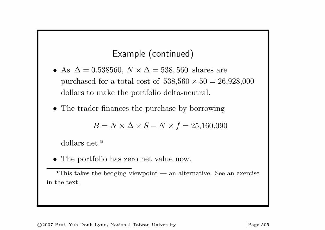
Example (continued)

• As ∆ = 0.538560, N ×∆ = 538, 560 shares arepurchased for a total cost of 538,560× 50 = 26,928,000dollars to make the portfolio delta-neutral.

• The trader finances the purchase by borrowing

B = N ×∆× S −N × f = 25,160,090

dollars net.a

• The portfolio has zero net value now.aThis takes the hedging viewpoint — an alternative. See an exercise

in the text.


Example (continued)

• At 3 weeks to expiration, the stock price rises to $51.

• The new call value is f ′ = 2.10580.

• So the portfolio is worth

−N × f ′ + 538,560× 51−Be0.06/52 = 171, 622

before rebalancing.


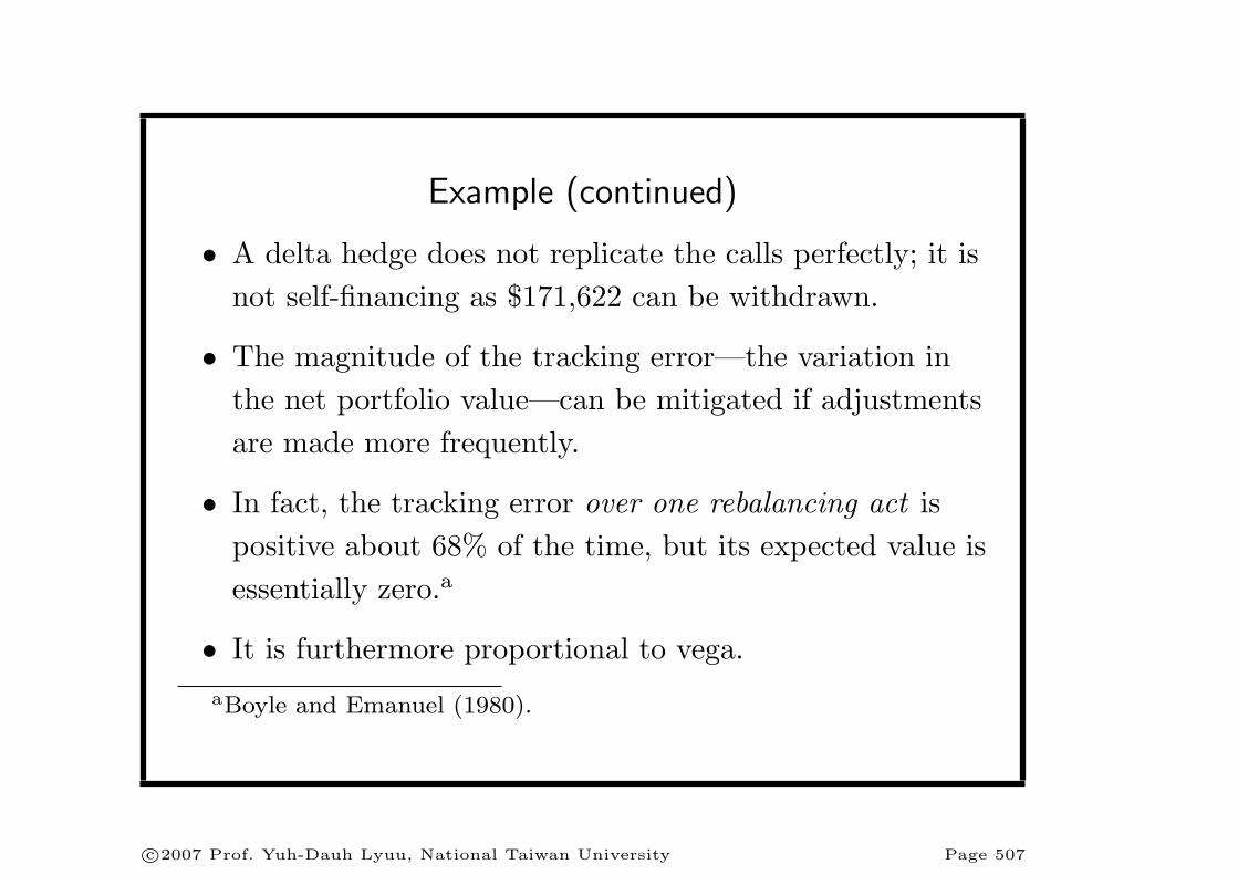
Example (continued)

• A delta hedge does not replicate the calls perfectly; it isnot self-financing as $171,622 can be withdrawn.

• The magnitude of the tracking error—the variation inthe net portfolio value—can be mitigated if adjustmentsare made more frequently.

• In fact, the tracking error over one rebalancing act ispositive about 68% of the time, but its expected value isessentially zero.a

• It is furthermore proportional to vega.aBoyle and Emanuel (1980).


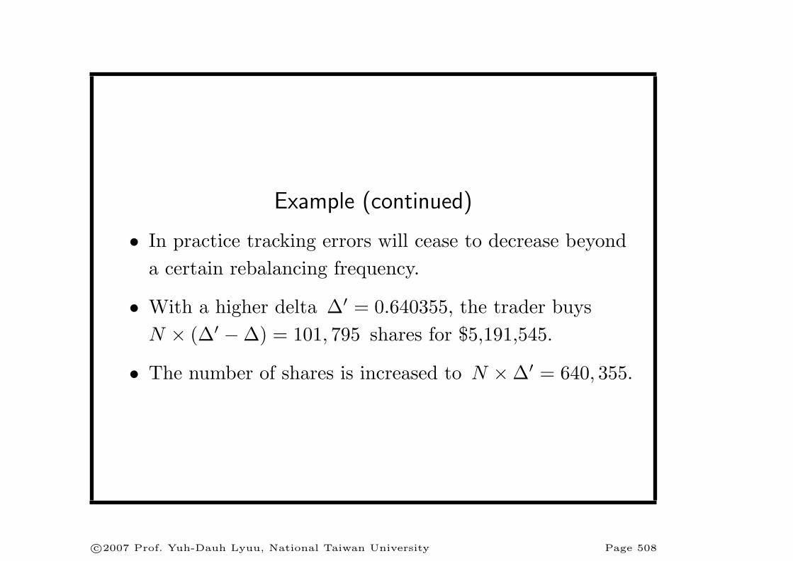
Example (continued)

• In practice tracking errors will cease to decrease beyonda certain rebalancing frequency.

• With a higher delta ∆′ = 0.640355, the trader buysN × (∆′ −∆) = 101, 795 shares for $5,191,545.

• The number of shares is increased to N ×∆′ = 640, 355.


Example (continued)

• The cumulative cost is

26,928,000× e0.06/52 + 5,191,545 = 32,150,634.

• The total borrowed amount is

B′ = 640,355× 51−N × f ′ = 30,552,305.

• The portfolio is again delta-neutral with zero value.


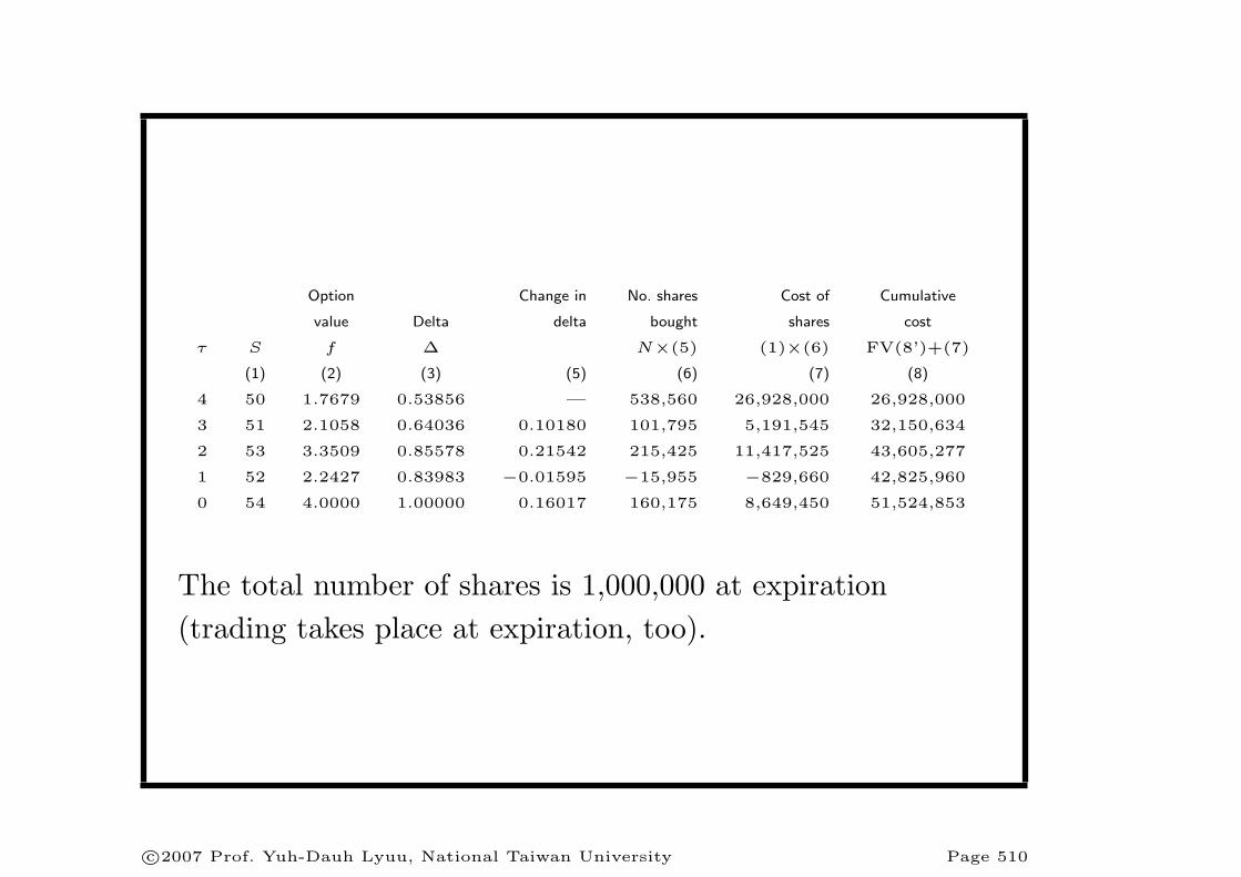
Option Change in No. shares Cost of Cumulative

value Delta delta bought shares cost

τ S f ∆ N×(5) (1)×(6) FV(8’)+(7)

(1) (2) (3) (5) (6) (7) (8)

4 50 1.7679 0.53856 — 538,560 26,928,000 26,928,000

3 51 2.1058 0.64036 0.10180 101,795 5,191,545 32,150,634

2 53 3.3509 0.85578 0.21542 215,425 11,417,525 43,605,277

1 52 2.2427 0.83983 −0.01595 −15,955 −829,660 42,825,960

0 54 4.0000 1.00000 0.16017 160,175 8,649,450 51,524,853

The total number of shares is 1,000,000 at expiration(trading takes place at expiration, too).


Example (concluded)

• At expiration, the trader has 1,000,000 shares.

• They are exercised against by the in-the-money calls for$50,000,000.

• The trader is left with an obligation of

51,524,853− 50,000,000 = 1,524,853,

which represents the replication cost.

• Compared with the FV of the call premium,

1,767,910× e0.06×4/52 = 1,776,088,

the net gain is 1,776,088− 1,524,853 = 251,235.


Tracking Error Revisiteda

• The tracking error εn over n rebalancing acts (such as251,235 above) has about the same probability of beingpositive as being negative.

• Subject to certain regularity conditions, theroot-mean-square tracking error

√E[ ε2n ] is O(1/

√n ).b

• The root-mean-square tracking error increases with σ atfirst and then decreases.

aBertsimas, Kogan, and Lo (2000).bSee also Grannan and Swindle (1996).


Delta-Gamma Hedge

• Delta hedge is based on the first-order approximation tochanges in the derivative price, ∆f , due to changes inthe stock price, ∆S.

• When ∆S is not small, the second-order term, gammaΓ ≡ ∂2f/∂S2, helps (theoretically).

• A delta-gamma hedge is a delta hedge that maintainszero portfolio gamma, or gamma neutrality.

• To meet this extra condition, one more security needs tobe brought in.


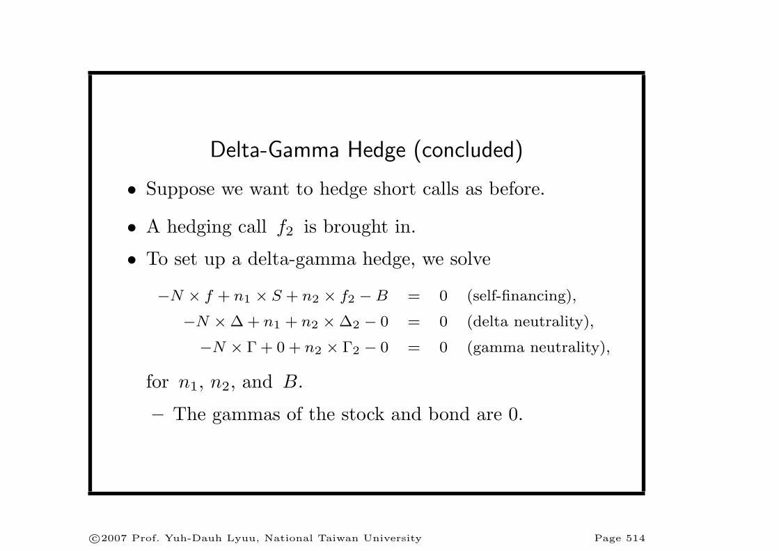
Delta-Gamma Hedge (concluded)

• Suppose we want to hedge short calls as before.

• A hedging call f2 is brought in.

• To set up a delta-gamma hedge, we solve

−N × f + n1 × S + n2 × f2 −B = 0 (self-financing),

−N ×∆ + n1 + n2 ×∆2 − 0 = 0 (delta neutrality),

−N × Γ + 0 + n2 × Γ2 − 0 = 0 (gamma neutrality),

for n1, n2, and B.

– The gammas of the stock and bond are 0.


Other Hedges

• If volatility changes, delta-gamma hedge may not workwell.

• An enhancement is the delta-gamma-vega hedge, whichalso maintains vega zero portfolio vega.

• To accomplish this, one more security has to be broughtinto the process.

• In practice, delta-vega hedge, which may not maintaingamma neutrality, performs better than delta hedge.


Trees


I love a tree more than a man.— Ludwig van Beethoven (1770–1827)

And though the holes were rather small,they had to count them all.

— The Beatles, A Day in the Life (1967)


The Combinatorial Method

• The combinatorial method can often cut the runningtime by an order of magnitude.

• The basic paradigm is to count the number of admissiblepaths that lead from the root to any terminal node.

• We first used this method in the linear-time algorithmfor standard European option pricing on p. 231.

– In general, it cannot apply to American options.

• We will now apply it to price barrier options.


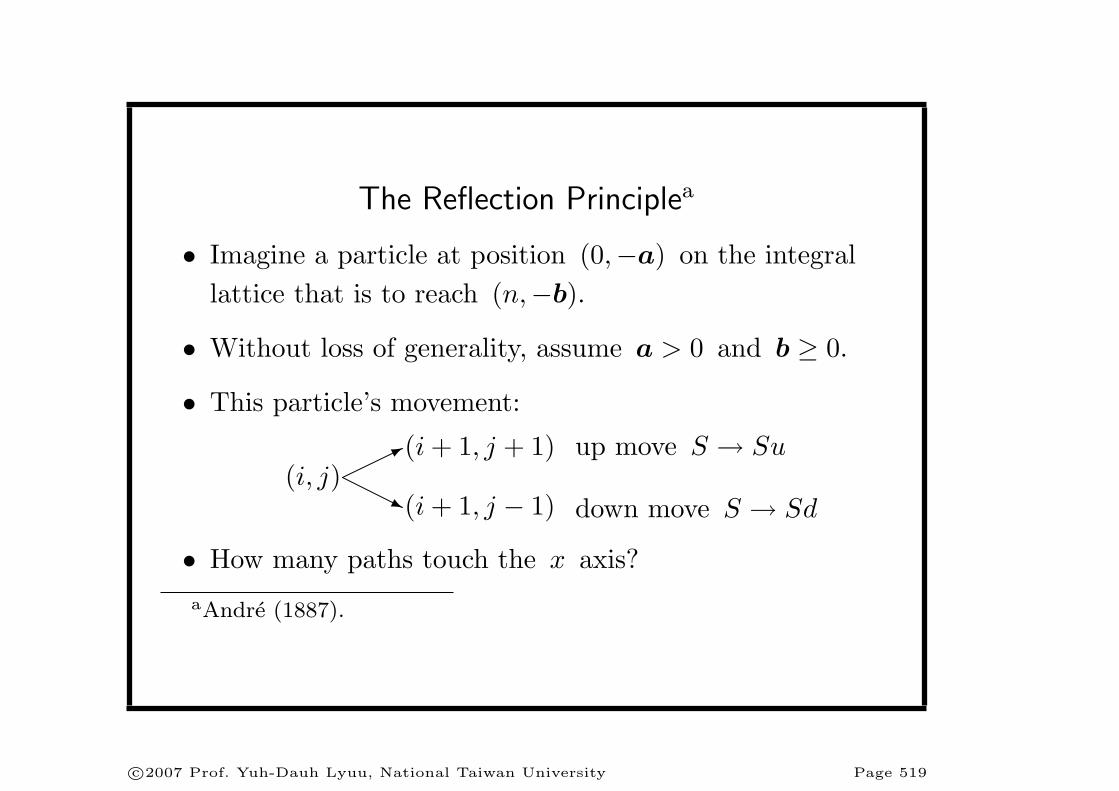
The Reflection Principlea

• Imagine a particle at position (0,−a) on the integrallattice that is to reach (n,−b).

• Without loss of generality, assume a > 0 and b ≥ 0.

• This particle’s movement:

(i, j)*(i + 1, j + 1) up move S → Su

j(i + 1, j − 1) down move S → Sd

• How many paths touch the x axis?aAndre (1887).


(0, a) (n, b)

(0, a)

J


The Reflection Principle (continued)

• For a path from (0,−a) to (n,−b) that touches the x

axis, let J denote the first point this happens.

• Reflect the portion of the path from (0,−a) to J .

• A path from (0, a) to (n,−b) is constructed.

• It also hits the x axis at J for the first time.

• The one-to-one mapping shows the number of pathsfrom (0,−a) to (n,−b) that touch the x axis equalsthe number of paths from (0,a) to (n,−b).


The Reflection Principle (concluded)

• A path of this kind has (n + b + a)/2 down moves and(n− b− a)/2 up moves.

• Hence there are(

nn+a+b

2

)(54)

such paths for even n + a + b.

– Convention:(nk

)= 0 for k < 0 or k > n.


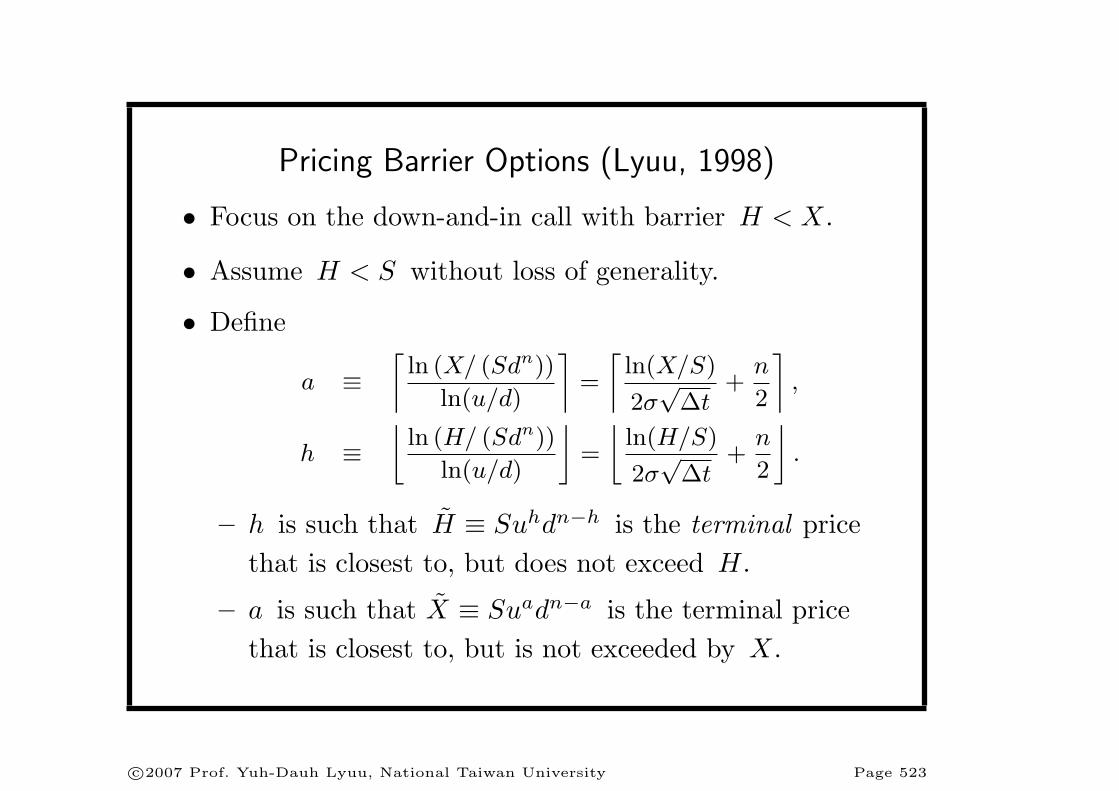
Pricing Barrier Options (Lyuu, 1998)

• Focus on the down-and-in call with barrier H < X.

• Assume H < S without loss of generality.

• Define

a ≡⌈

ln (X/ (Sdn))

ln(u/d)

⌉=

⌈ln(X/S)

2σ√

∆t+

n

2

⌉,

h ≡⌊

ln (H/ (Sdn))

ln(u/d)

⌋=

⌊ln(H/S)

2σ√

∆t+

n

2

⌋.

– h is such that H ≡ Suhdn−h is the terminal pricethat is closest to, but does not exceed H.

– a is such that X ≡ Suadn−a is the terminal pricethat is closest to, but is not exceeded by X.


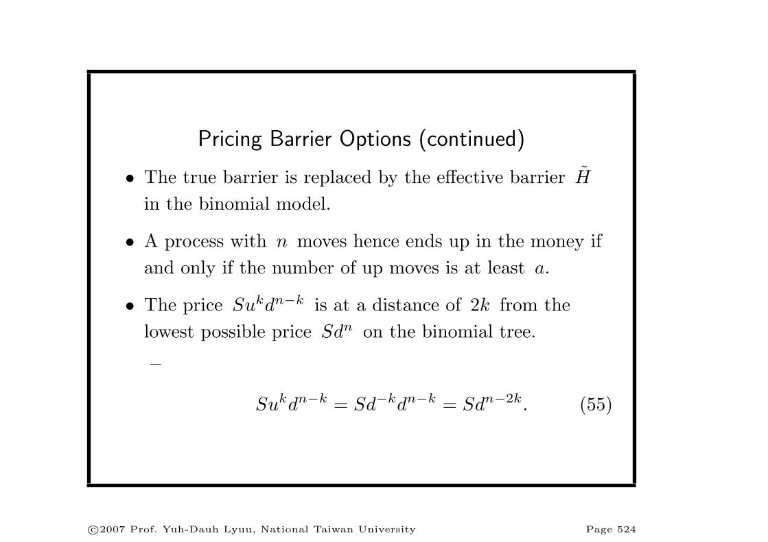
Pricing Barrier Options (continued)

• The true barrier is replaced by the effective barrier H

in the binomial model.

• A process with n moves hence ends up in the money ifand only if the number of up moves is at least a.

• The price Sukdn−k is at a distance of 2k from thelowest possible price Sdn on the binomial tree.

–

Sukdn−k = Sd−kdn−k = Sdn−2k. (55)


0

0

2 hn2 a

S

0

0

0

0

2 j

~X Su da n a

Su dj n j

~H Su dh n h


Pricing Barrier Options (continued)

• The number of paths from S to the terminal priceSujdn−j is

(nj

), each with probability pj(1− p)n−j .

• With reference to p. 525, the reflection principle can beapplied with a = n− 2h and b = 2j − 2h in Eq. (54)on p. 522 by treating the S line as the x axis.

• Therefore,(

nn+(n−2h)+(2j−2h)

2

)=

(n

n− 2h + j

)

paths hit H in the process for h ≤ n/2.


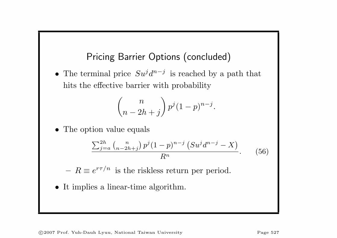
Pricing Barrier Options (concluded)

• The terminal price Sujdn−j is reached by a path thathits the effective barrier with probability

(n

n− 2h + j

)pj(1− p)n−j .

• The option value equals∑2h

j=a

(n

n−2h+j

)pj(1− p)n−j

(Sujdn−j −X

)

Rn. (56)

– R ≡ erτ/n is the riskless return per period.

• It implies a linear-time algorithm.


Convergence of BOPM

• Equation (56) results in the sawtooth-like convergenceshown on p. 310.

• The reasons are not hard to see.

• The true barrier most likely does not equal the effectivebarrier.

• The same holds for the strike price and the effectivestrike price.

• The issue of the strike price is less critical.

• But the issue of the barrier is not negligible.


Convergence of BOPM (continued)

• Convergence is actually good if we limit n to certainvalues—191, for example.

• These values make the true barrier coincide with oroccur just above one of the stock price levels, that is,H ≈ Sdj = Se−jσ

√τ/n for some integer j.

• The preferred n’s are thus

n =

⌊τ

(ln(S/H)/(jσ))2

⌋, j = 1, 2, 3, . . .

• There is only one minor technicality left.


Convergence of BOPM (continued)

• We picked the effective barrier to be one of the n + 1possible terminal stock prices.

• However, the effective barrier above, Sdj , corresponds toa terminal stock price only when n− j is even byEq. (55) on p. 524.a

• To close this gap, we decrement n by one, if necessary,to make n− j an even number.

aWe could have adopted the form Sdj (−n ≤ j ≤ n) for the effective

barrier.


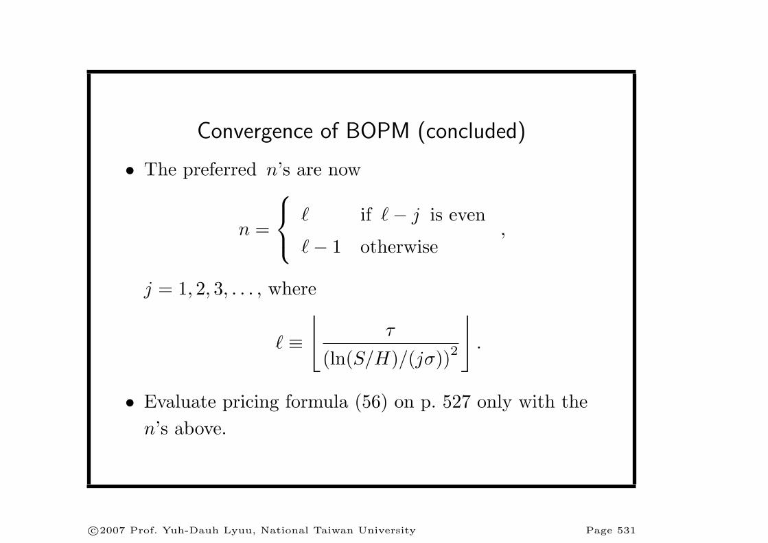
Convergence of BOPM (concluded)

• The preferred n’s are now

n =

` if `− j is even

`− 1 otherwise,

j = 1, 2, 3, . . . , where

` ≡⌊

τ

(ln(S/H)/(jσ))2

⌋.

• Evaluate pricing formula (56) on p. 527 only with then’s above.


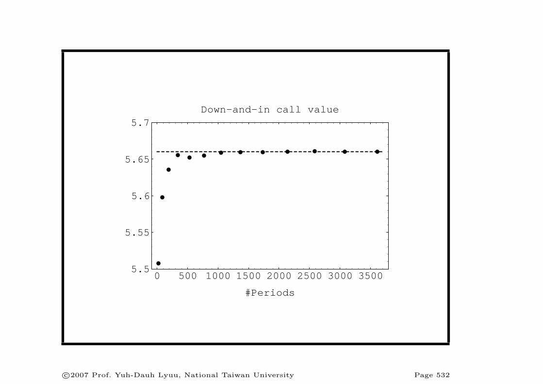
0 500 1000 1500 2000 2500 3000 3500

#Periods

5.5

5.55

5.6

5.65

5.7

Down-and-in call value


Practical Implications

• Now that barrier options can be efficiently priced, wecan afford to pick very large n’s (p. 534).

• This has profound consequences.


n Combinatorial method

Value Time (milliseconds)

21 5.507548 0.30

84 5.597597 0.90

191 5.635415 2.00

342 5.655812 3.60

533 5.652253 5.60

768 5.654609 8.00

1047 5.658622 11.10

1368 5.659711 15.00

1731 5.659416 19.40

2138 5.660511 24.70

2587 5.660592 30.20

3078 5.660099 36.70

3613 5.660498 43.70

4190 5.660388 44.10

4809 5.659955 51.60

5472 5.660122 68.70

6177 5.659981 76.70

6926 5.660263 86.90

7717 5.660272 97.20


Practical Implications (concluded)

• Pricing is prohibitively time consuming when S ≈ H

because n ∼ 1/ ln2(S/H).

• This observation is indeed true of standardquadratic-time binomial tree algorithms.

• But it no longer applies to linear-time algorithms(p. 536).


Barrier at 95.0 Barrier at 99.5 Barrier at 99.9

n Value Time n Value Time n Value Time

.

.

. 795 7.47761 8 19979 8.11304 253

2743 2.56095 31.1 3184 7.47626 38 79920 8.11297 1013

3040 2.56065 35.5 7163 7.47682 88 179819 8.11300 2200

3351 2.56098 40.1 12736 7.47661 166 319680 8.11299 4100

3678 2.56055 43.8 19899 7.47676 253 499499 8.11299 6300

4021 2.56152 48.1 28656 7.47667 368 719280 8.11299 8500

True 2.5615 7.4767 8.1130

(All times in milliseconds.)


Trinomial Tree

• Set up a trinomial approximation to the geometricBrownian motion dS/S = r dt + σ dW .a

• The three stock prices at time ∆t are S, Su, and Sd,where ud = 1.

• Impose the matching of mean and that of variance:

1 = pu + pm + pd,

SM ≡ (puu + pm + (pd/u)) S,

S2V ≡ pu(Su− SM)2 + pm(S − SM)2 + pd(Sd− SM)2.

aBoyle (1988).


• Above,

M ≡ er∆t,

V ≡ M2(eσ2∆t − 1),

by Eqs. (17) on p. 147.


*

-

j

pu

pm

pd

Su

S

Sd

S

-¾∆t

*

-

j

*

-

j

*

-

j

*

-

j


Trinomial Tree (continued)

• Use linear algebra to verify that

pu =u

(V + M2 −M

)− (M − 1)(u− 1) (u2 − 1)

,

pd =u2

(V + M2 −M

)− u3(M − 1)(u− 1) (u2 − 1)

.

– In practice, must make sure the probabilities liebetween 0 and 1.

• Countless variations.


Trinomial Tree (concluded)

• Use u = eλσ√

∆t, where λ ≥ 1 is a tunable parameter.

• Then

pu → 12λ2

+

(r + σ2

)√∆t

2λσ,

pd → 12λ2

−(r − 2σ2

)√∆t

2λσ.

• A nice choice for λ is√

π/2 .a

aOmberg (1988).


Barrier Options Revisited

• BOPM introduces a specification error by replacing thebarrier with a nonidentical effective barrier.

• The trinomial model solves the problem by adjusting λ

so that the barrier is hit exactly.a

• It takes

h =ln(S/H)λσ√

∆t

consecutive down moves to go from S to H if h is aninteger, which is easy to achieve by adjusting λ.

– This is because Se−hλσ√

∆t = H.aRitchken (1995).


Barrier Options Revisited (continued)

• Typically, we find the smallest λ ≥ 1 such that h is aninteger.

• That is, we find the largest integer j ≥ 1 that satisfiesln(S/H)

jσ√

∆t≥ 1 and then let

λ =ln(S/H)jσ√

∆t.

– Such a λ may not exist for very small n’s.

– This is not hard to check.

• This done, one of the layers of the trinomial treecoincides with the barrier.


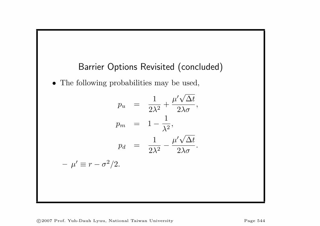
Barrier Options Revisited (concluded)

• The following probabilities may be used,

pu =1

2λ2+

µ′√

∆t

2λσ,

pm = 1− 1λ2

,

pd =1

2λ2− µ′

√∆t

2λσ.

– µ′ ≡ r − σ2/2.


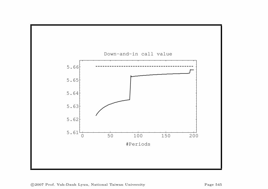
0 50 100 150 200

#Periods

5.61

5.62

5.63

5.64

5.65

5.66

Down-and-in call value


Algorithms Comparisona

• So which algorithm is better, binomial or trinomial?

• Algorithms are often compared based on the n value atwhich they converge.

– The one with the smallest n wins.

• So giraffes are faster than cheetahs because they takefewer strides to travel the same distance!

• Performance must be based on actual running times.aLyuu (1998).


Algorithms Comparison (concluded)

• Pages 310 and 545 show the trinomial model convergesat a smaller n than BOPM.

• It is in this sense when people say trinomial modelsconverge faster than binomial ones.

• But is the trinomial model better then?

• The linear-time binomial tree algorithm actuallyperforms better than the trinomial one (see next pageexpanded from p. 534).


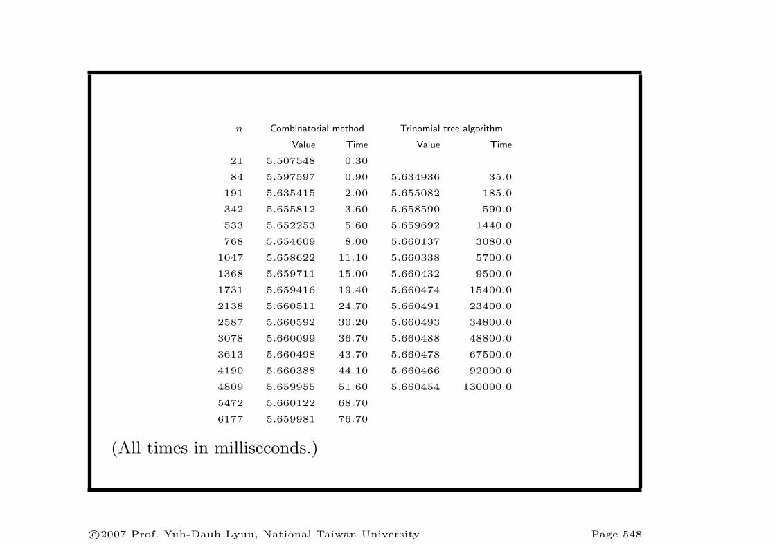
n Combinatorial method Trinomial tree algorithm

Value Time Value Time

21 5.507548 0.30

84 5.597597 0.90 5.634936 35.0

191 5.635415 2.00 5.655082 185.0

342 5.655812 3.60 5.658590 590.0

533 5.652253 5.60 5.659692 1440.0

768 5.654609 8.00 5.660137 3080.0

1047 5.658622 11.10 5.660338 5700.0

1368 5.659711 15.00 5.660432 9500.0

1731 5.659416 19.40 5.660474 15400.0

2138 5.660511 24.70 5.660491 23400.0

2587 5.660592 30.20 5.660493 34800.0

3078 5.660099 36.70 5.660488 48800.0

3613 5.660498 43.70 5.660478 67500.0

4190 5.660388 44.10 5.660466 92000.0

4809 5.659955 51.60 5.660454 130000.0

5472 5.660122 68.70

6177 5.659981 76.70

(All times in milliseconds.)


Double-Barrier Options

• Double-barrier options are barrier options with twobarriers L < H.

• Assume L < S < H.

• The binomial model produces oscillating option values(see plot next page).a

aChao (1999); Dai and Lyuu (2005);


20 40 60 80 100

8

10

12

14

16


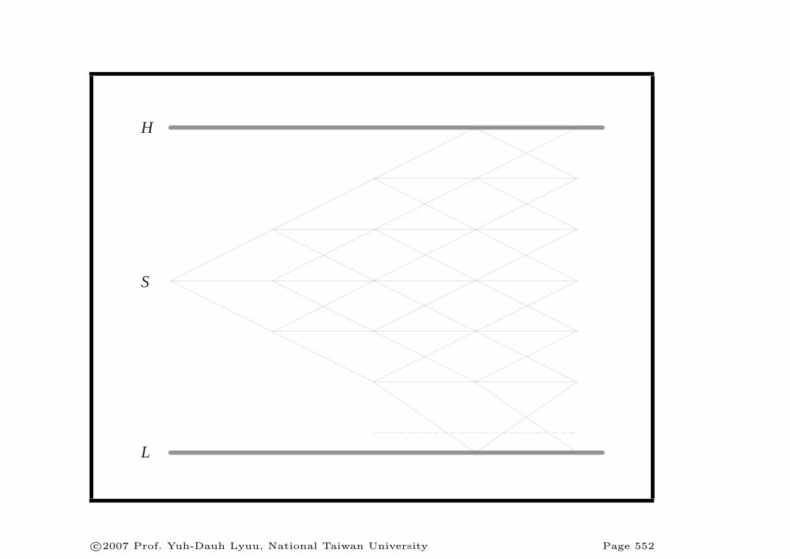
Double-Barrier Knock-Out Options

• We knew how to pick the λ so that one of the layers ofthe trinomial tree coincides with one barrier, say H.

• This choice, however, does not guarantee that the otherbarrier, L, is also hit.

• One way to handle this problem is to lower the layer ofthe tree just above L to coincide with L.a

– More general ways to make the trinomial model hitboth barriers are available.b

aRitchken (1995).bHsu and Lyuu (2006). Dai and Lyuu (2006) combine binomial and

trinomial trees to derive an O(n)-time algorithm for double-barrier op-

tions!


H

L

S


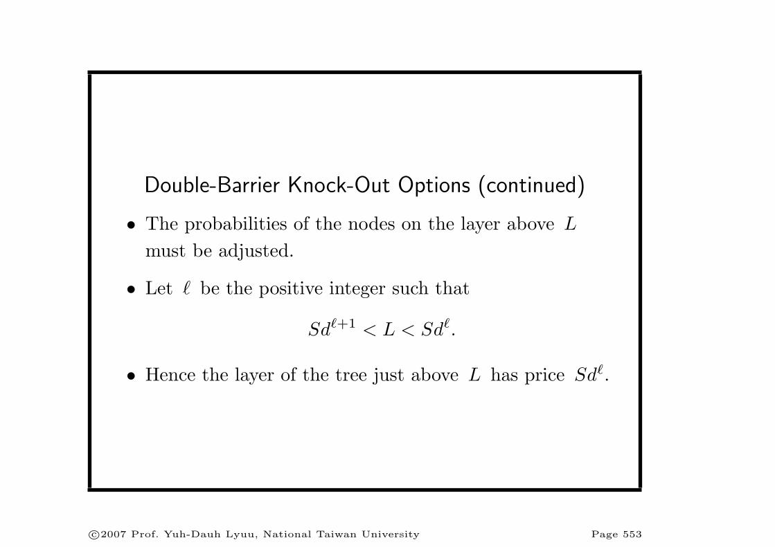
Double-Barrier Knock-Out Options (continued)

• The probabilities of the nodes on the layer above L

must be adjusted.

• Let ` be the positive integer such that

Sd`+1 < L < Sd`.

• Hence the layer of the tree just above L has price Sd`.


Double-Barrier Knock-Out Options (concluded)

• Define γ > 1 as the number satisfying

L = Sd`−1e−γλσ√

∆t.

– The prices between the barriers are

L, Sd`−1, . . . , Sd2, Sd, S, Su, Su2, . . . , Suh−1, Suh = H.

• The probabilities for the nodes with price equal toSd`−1 are

p′u =b + aγ

1 + γ, p′d =

b− a

γ + γ2, and p′m = 1− p′u − p′d,

where a ≡ µ′√

∆t/(λσ) and b ≡ 1/λ2.

c©2007 Prof. Yuh-Dauh Lyuu, National Taiwan University 4

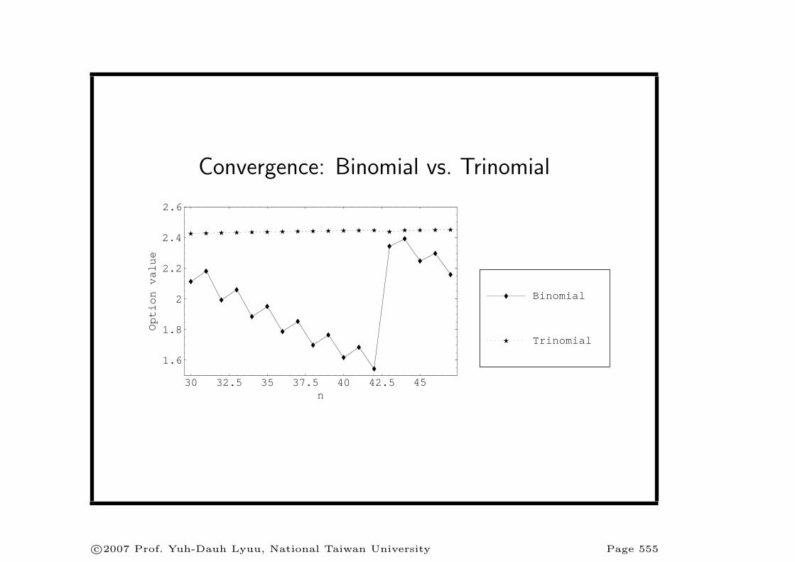
Convergence: Binomial vs. Trinomial

30 32.5 35 37.5 40 42.5 45n

1.6

1.8

2

2.2

2.4

2.6

Option

value

Trinomial

Binomial


Delta Hedge - 國立臺灣大學lyuu/finance1/2007/20070509.pdf · Delta Hedge (concluded) †...

Documents

Transcript of Delta Hedge - 國立臺灣大學lyuu/finance1/2007/20070509.pdf · Delta Hedge (concluded) †...