Deep Monitoring of On- and Offshore Projects -...
51
Deep Monitoring of On- and Offshore Projects Dr Matthias Raab IEAGHG Summer School 8 December 2015
Transcript of Deep Monitoring of On- and Offshore Projects -...
Deep Monitoring of On- and Offshore Projects
Dr Matthias Raab
IEAGHG Summer School8 December 2015
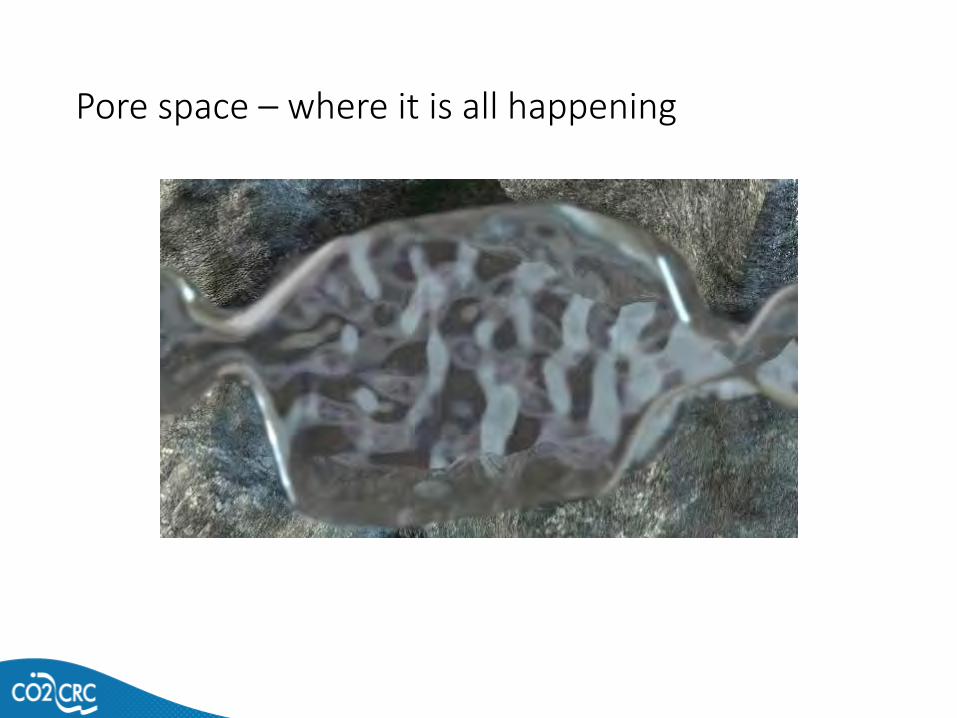
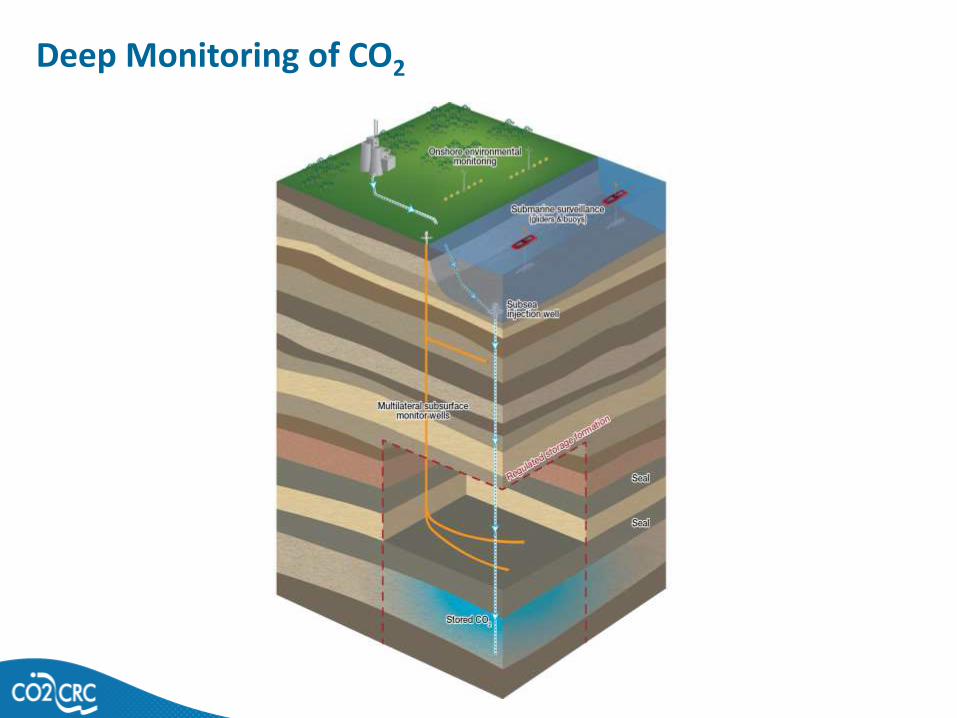
Pore space – where it is all happening
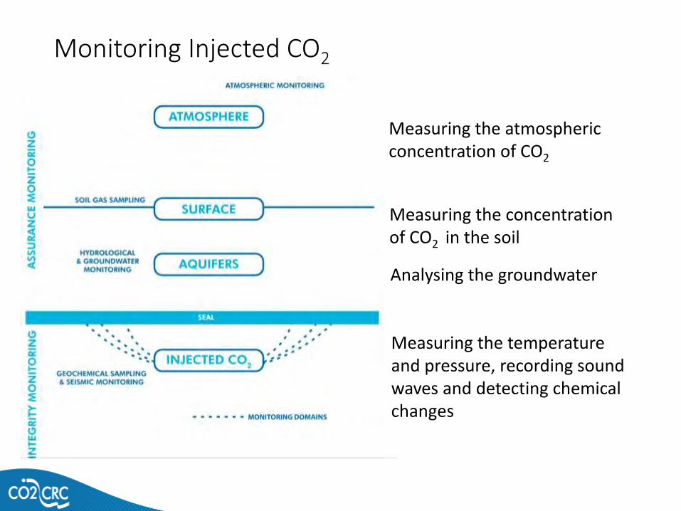
Measuring the atmospheric concentration of CO2
Measuring the concentration of CO2 in the soil
Measuring the temperature and pressure, recording sound waves and detecting chemical changes
Analysing the groundwater
Monitoring Injected CO2
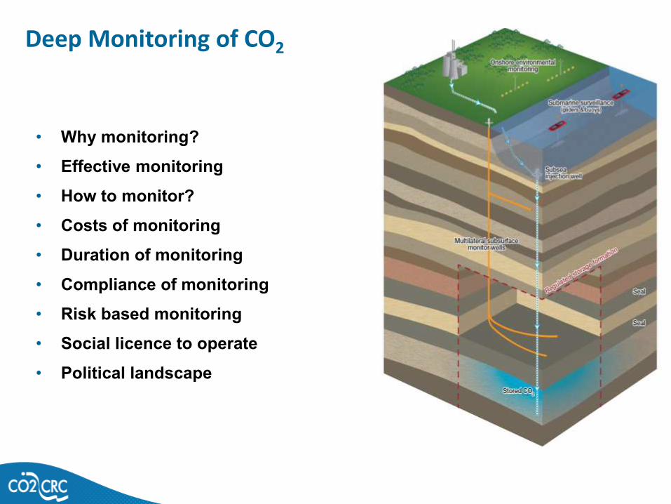
• Why monitoring?• Effective monitoring• How to monitor?• Costs of monitoring• Duration of monitoring• Compliance of monitoring• Risk based monitoring• Social licence to operate• Political landscape
Deep Monitoring of CO2
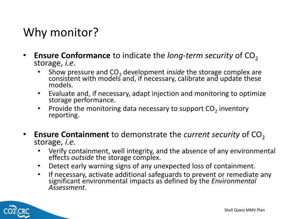
Why monitor?
• Ensure Conformance to indicate the long-term security of CO2storage, i.e. • Show pressure and CO2 development inside the storage complex are
consistent with models and, if necessary, calibrate and update these models.
• Evaluate and, if necessary, adapt injection and monitoring to optimize storage performance.
• Provide the monitoring data necessary to support CO2 inventory reporting.
• Ensure Containment to demonstrate the current security of CO2storage, i.e. • Verify containment, well integrity, and the absence of any environmental
effects outside the storage complex. • Detect early warning signs of any unexpected loss of containment. • If necessary, activate additional safeguards to prevent or remediate any
significant environmental impacts as defined by the Environmental Assessment.
Shell Quest MMV Plan
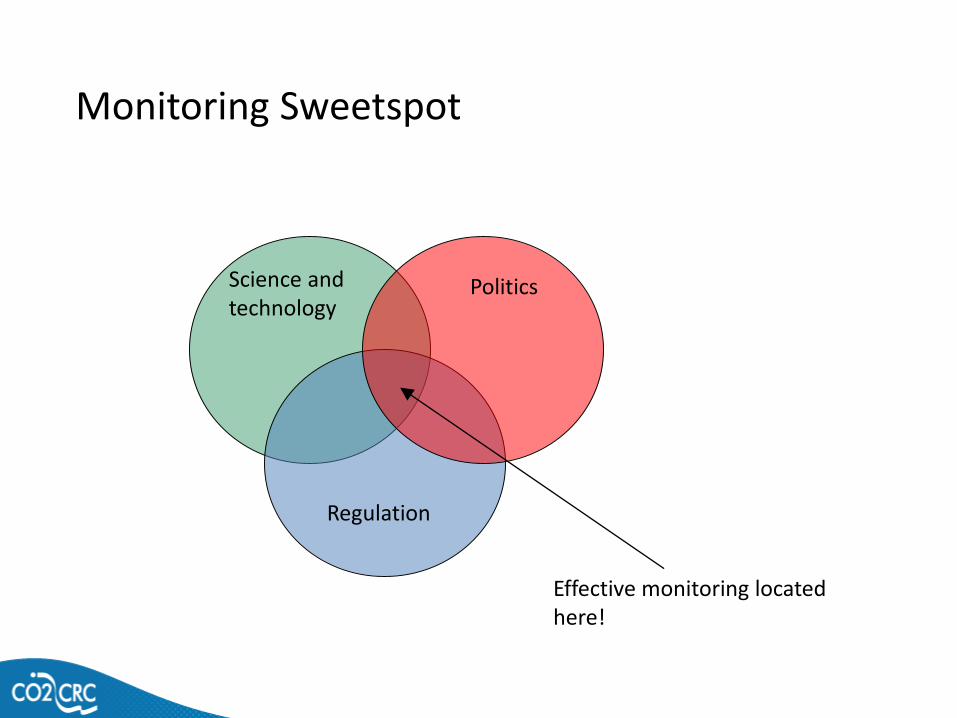
Monitoring Sweetspot
Science and technology
Regulation
Politics
Effective monitoring located here!
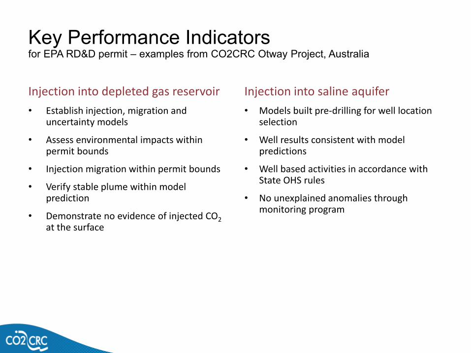
Key Performance Indicators for EPA RD&D permit – examples from CO2CRC Otway Project, Australia
Injection into depleted gas reservoir
• Establish injection, migration and uncertainty models
• Assess environmental impacts within permit bounds
• Injection migration within permit bounds
• Verify stable plume within model prediction
• Demonstrate no evidence of injected CO2
at the surface
Injection into saline aquifer
• Models built pre-drilling for well location selection
• Well results consistent with model predictions
• Well based activities in accordance with State OHS rules
• No unexplained anomalies through monitoring program
Risk Based Approach to Monitoring
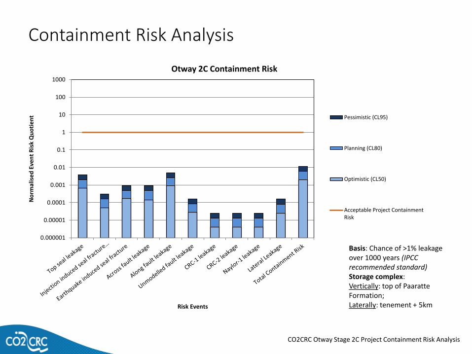
Containment Risk Analysis
0.000001
0.00001
0.0001
0.001
0.01
0.1
1
10
100
1000
No
rmal
ise
d E
ven
t R
isk
Qu
oti
en
t
Risk Events
Otway 2C Containment Risk
Pessimistic (CL95)
Planning (CL80)
Optimistic (CL50)
Acceptable Project ContainmentRisk
Basis: Chance of >1% leakage over 1000 years (IPCC recommended standard)Storage complex: Vertically: top of Paaratte Formation; Laterally: tenement + 5km
CO2CRC Otway Stage 2C Project Containment Risk Analysis
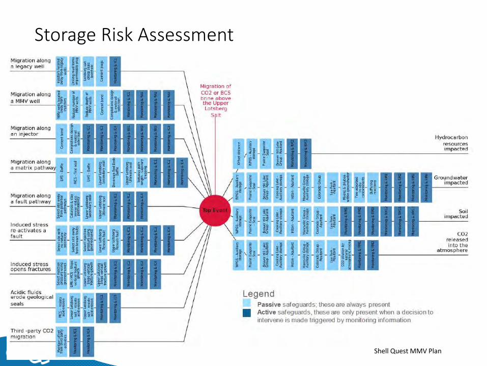
Storage Risk Assessment
Shell Quest MMV Plan
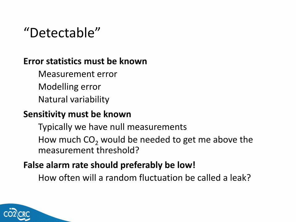
“Detectable”
Error statistics must be known
Measurement error
Modelling error
Natural variability
Sensitivity must be known
Typically we have null measurements
How much CO2 would be needed to get me above the measurement threshold?
False alarm rate should preferably be low!
How often will a random fluctuation be called a leak?
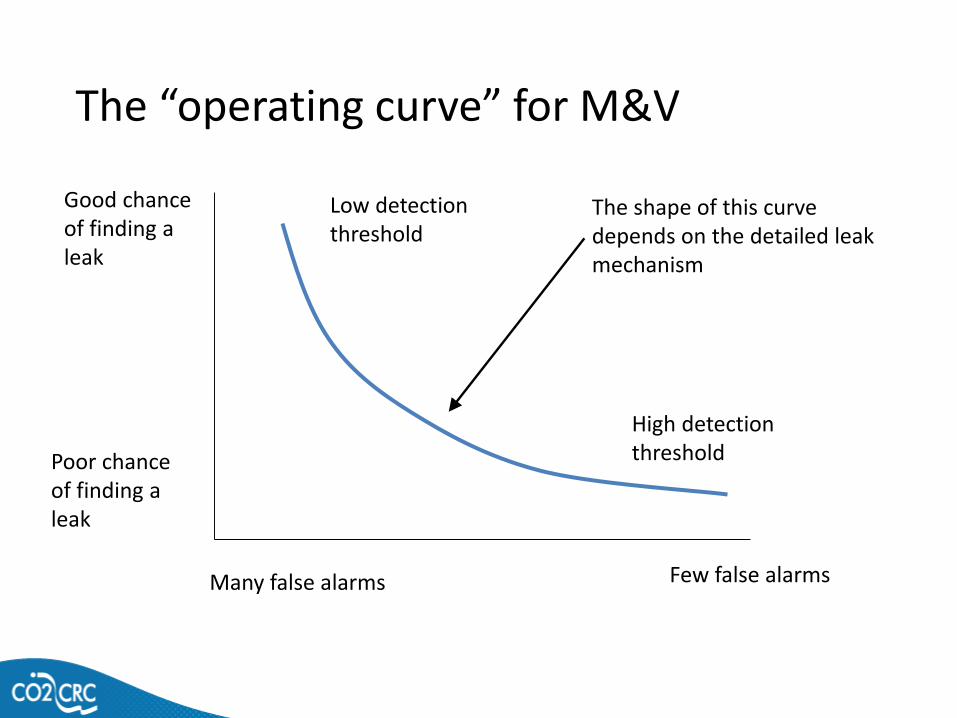
The “operating curve” for M&V
Many false alarms Few false alarms
Good chance of finding a leak
Poor chance of finding a leak
Low detection threshold
High detection threshold
The shape of this curve depends on the detailed leak mechanism
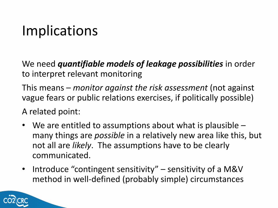
Implications
We need quantifiable models of leakage possibilities in order to interpret relevant monitoring
This means – monitor against the risk assessment (not against vague fears or public relations exercises, if politically possible)
A related point:
• We are entitled to assumptions about what is plausible –many things are possible in a relatively new area like this, but not all are likely. The assumptions have to be clearly communicated.
• Introduce “contingent sensitivity” – sensitivity of a M&V method in well-defined (probably simple) circumstances
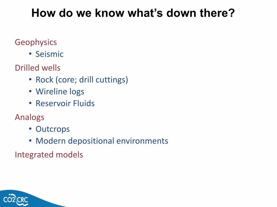
Geophysics
• Seismic
Drilled wells
• Rock (core; drill cuttings)
• Wireline logs
• Reservoir Fluids
Analogs
• Outcrops
• Modern depositional environments
Integrated models
How do we know what’s down there?
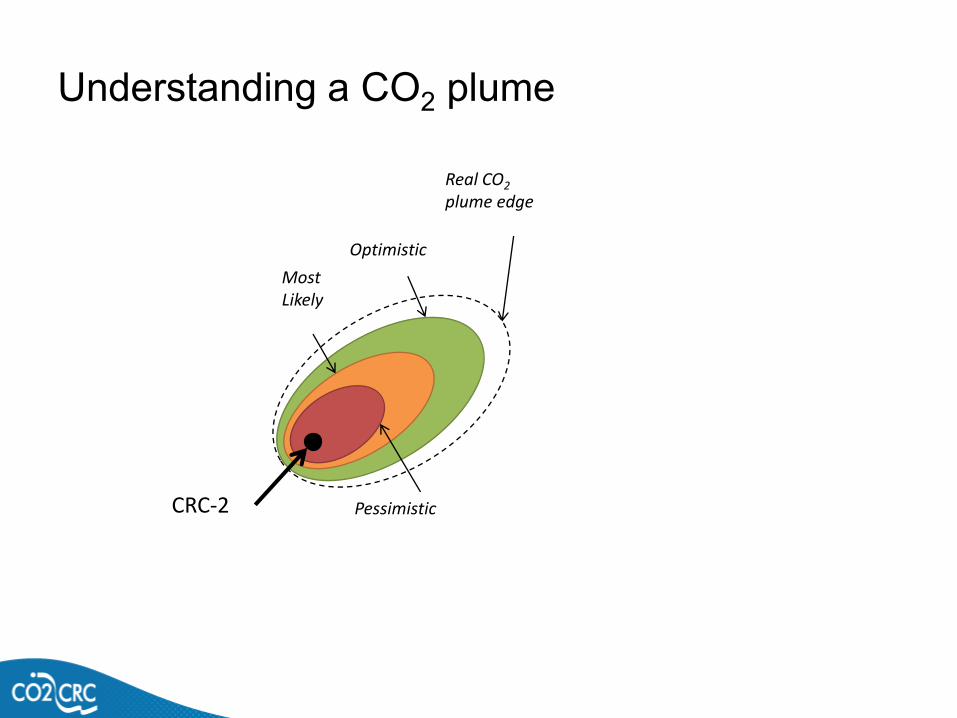
Understanding a CO2 plume
Pessimistic
MostLikely
Optimistic
Real CO2
plume edge
CRC-2
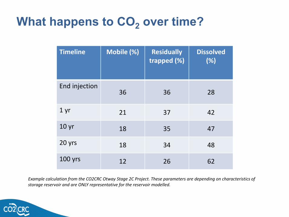
What happens to CO2 over time?
Timeline Mobile (%) Residually trapped (%)
Dissolved (%)
End injection36 36 28
1 yr 21 37 42
10 yr 18 35 47
20 yrs 18 34 48
100 yrs 12 26 62
Example calculation from the CO2CRC Otway Stage 2C Project. These parameters are depending on characteristics of storage reservoir and are ONLY representative for the reservoir modelled.
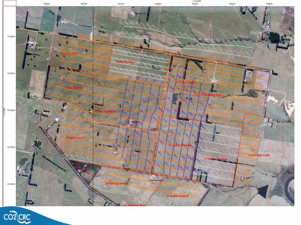
Onshore Seismic Monitoring
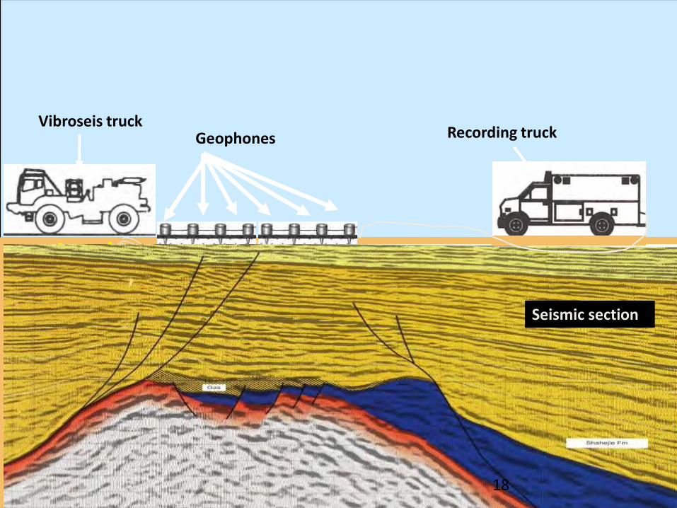
GeophonesVibroseis truck
Recording truck
Seismic section
18

Seismic-source: Vibrator Truck
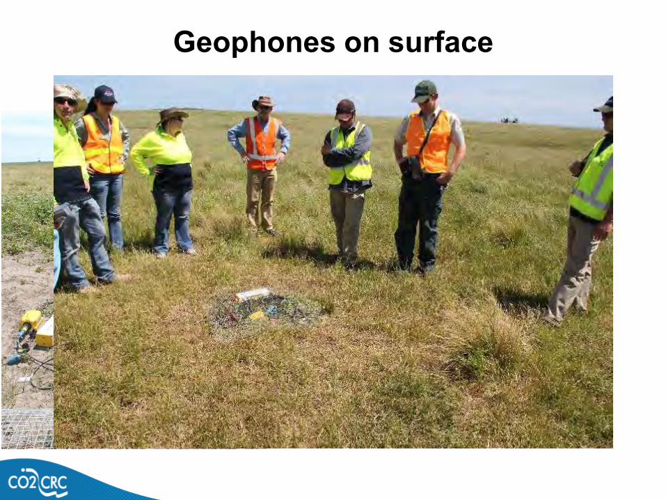
Geophones on surface
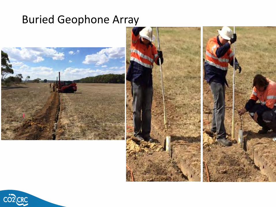
Buried Geophone Array
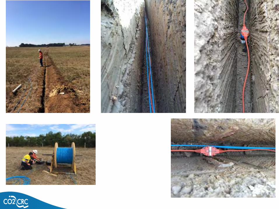
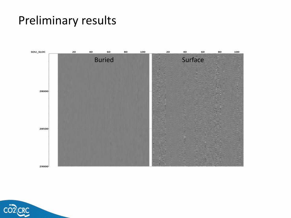
Preliminary results
Buried Surface

Offshore Seismic Monitoring
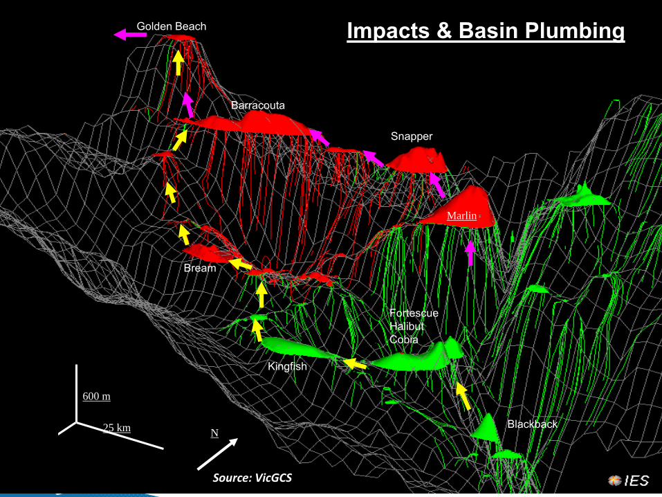
Western
Kitchen
(Type III)Central
Kitchen
(Type II)
Eastern
Kitchen
(Type II)
Western
Kitchen
(Type III)Central
Kitchen
(Type II)
Eastern
Kitchen
(Type II)
FortescueHalibutCobia
Kingfish
Blackback
Marlin
Snapper
Barracouta
Golden Beach Present (0 Ma)
Bream
25 km25 km
600 m
N
Impacts & Basin Plumbing
Source: VicGCS
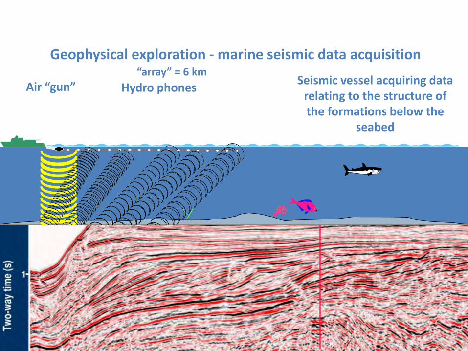
Seismic vessel acquiring data relating to the structure of the formations below the
seabed
Air “gun” Hydro phones“array” = 6 km
Geophysical exploration - marine seismic data acquisition

2D Vessel Aquila Explorer
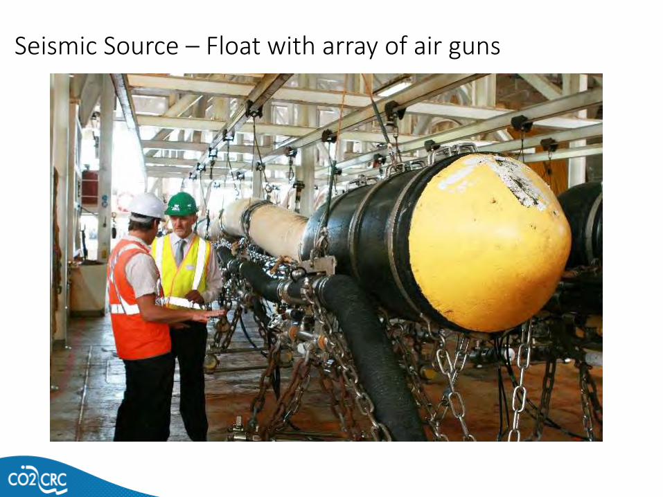
Seismic Source – Float with array of air guns
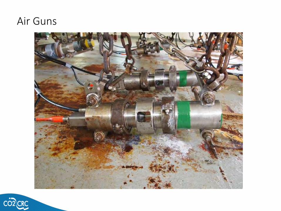
Air Guns
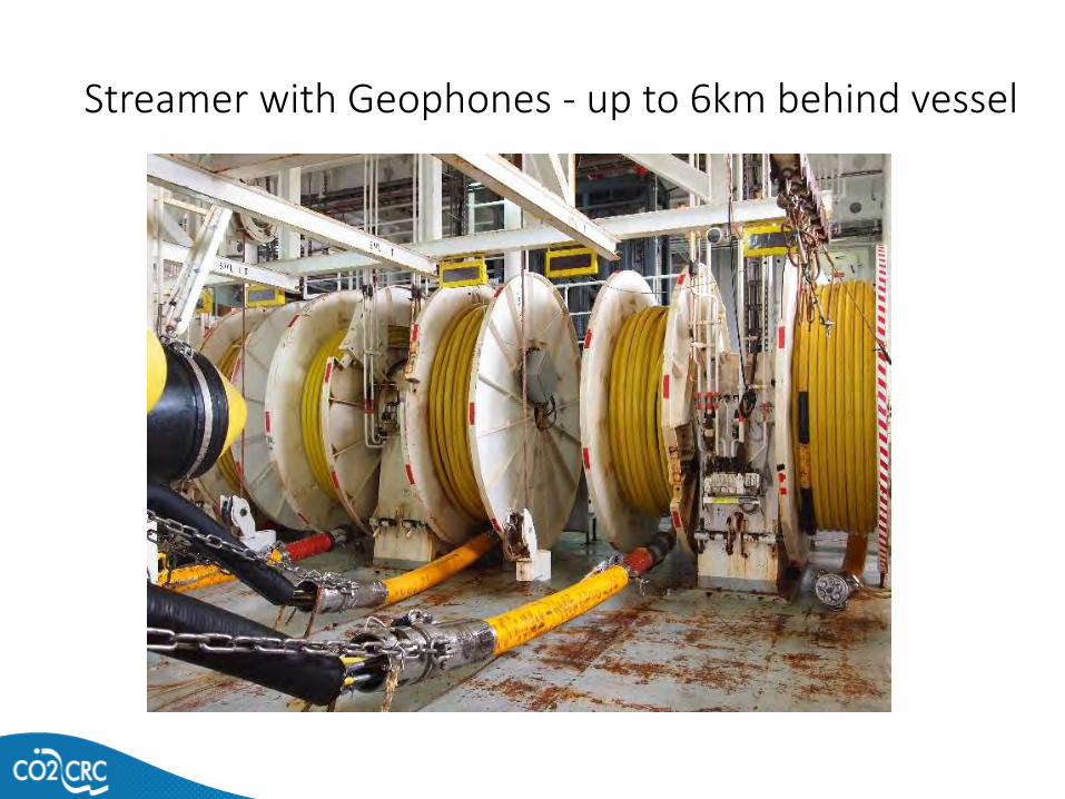
Streamer with Geophones - up to 6km behind vessel
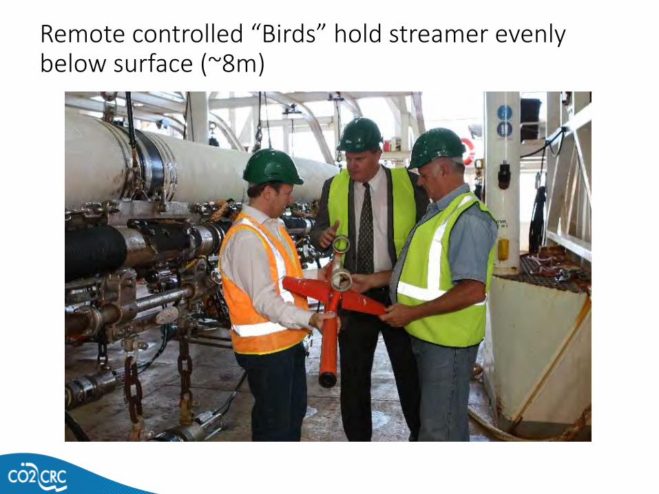
Remote controlled “Birds” hold streamer evenly below surface (~8m)
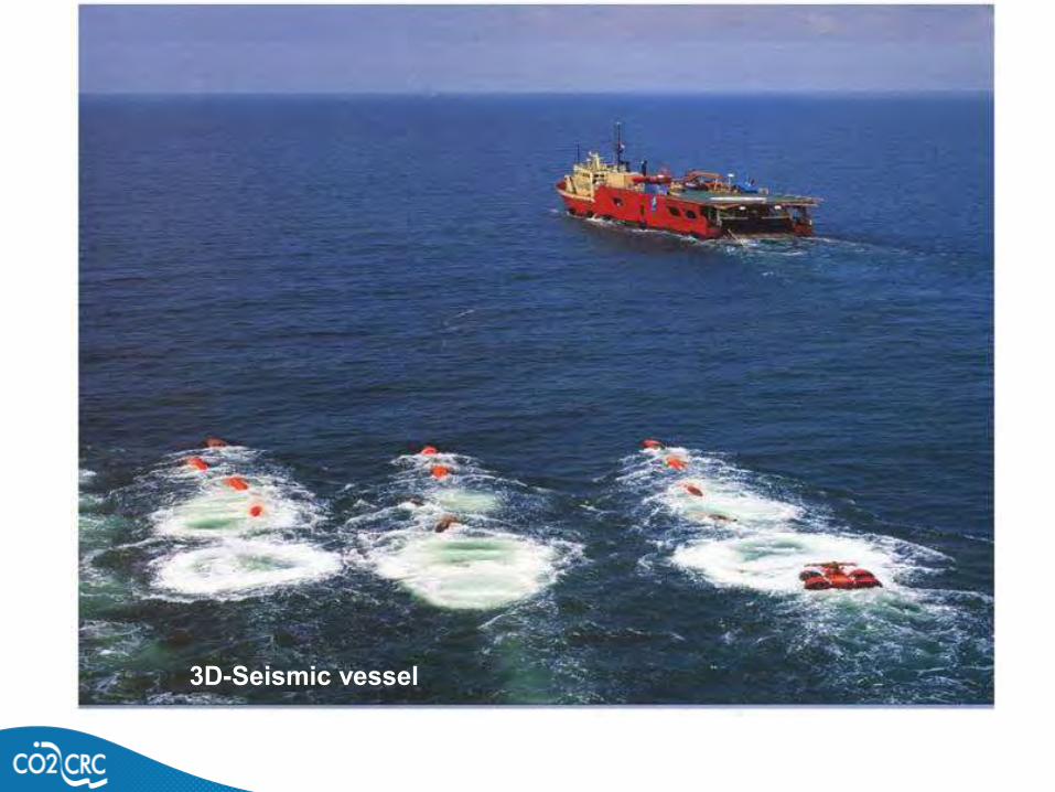
3D-Seismic vessel
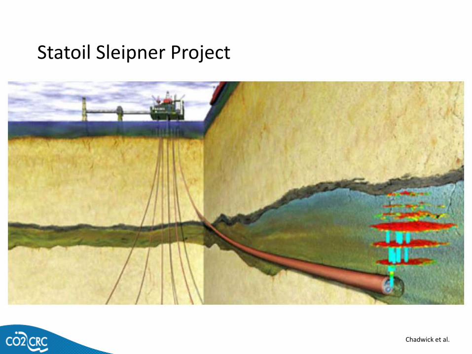
Statoil Sleipner Project
Chadwick et al.
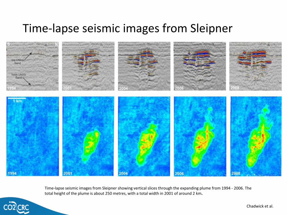
Time-lapse seismic images from Sleipner
Time-lapse seismic images from Sleipner showing vertical slices through the expanding plume from 1994 - 2006. The total height of the plume is about 250 metres, with a total width in 2001 of around 2 km.
Chadwick et al.
Chadwick et al.
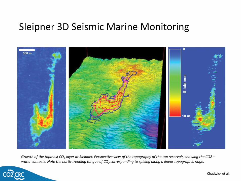
Growth of the topmost CO2 layer at Sleipner. Perspective view of the topography of the top reservoir, showing the CO2 –water contacts. Note the north-trending tongue of CO2 corresponding to spilling along a linear topographic ridge.
Sleipner 3D Seismic Marine Monitoring

InSAR Monitoring
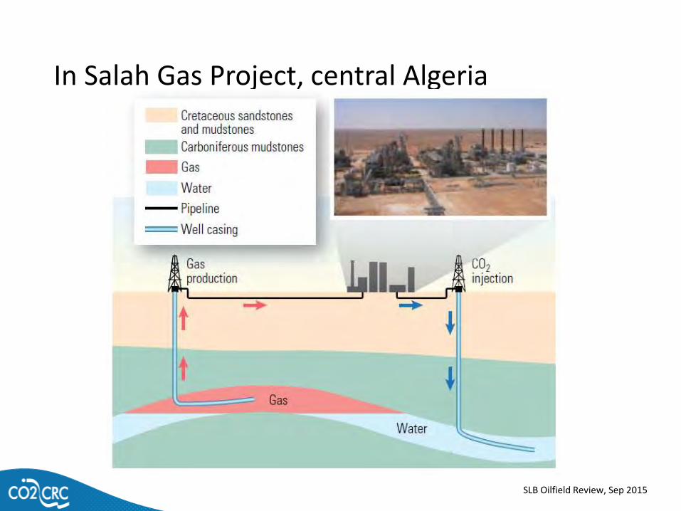
In Salah Gas Project, central Algeria
SLB Oilfield Review, Sep 2015
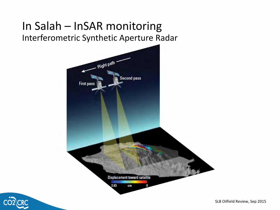
In Salah – InSAR monitoringInterferometric Synthetic Aperture Radar
SLB Oilfield Review, Sep 2015
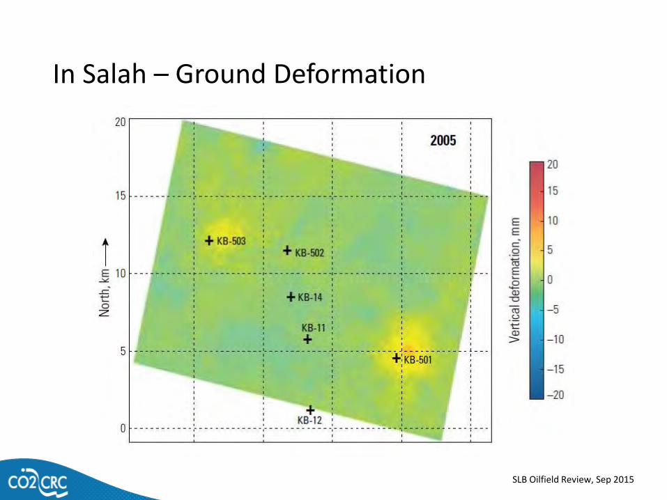
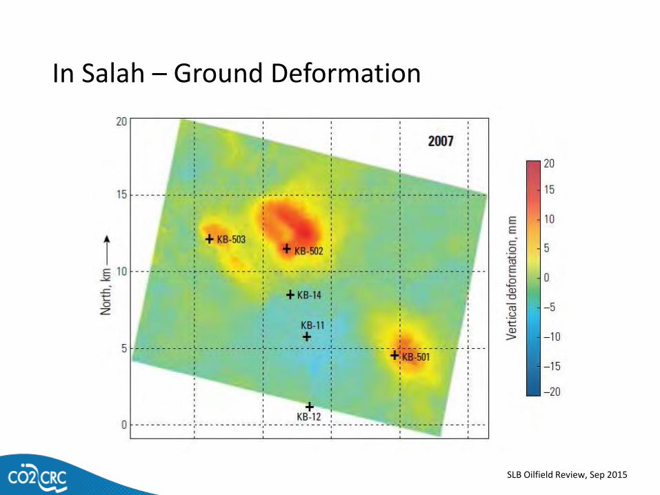
In Salah – Ground Deformation
SLB Oilfield Review, Sep 2015
In Salah – Ground Deformation
SLB Oilfield Review, Sep 2015
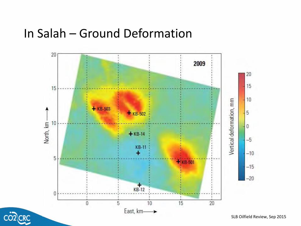
In Salah – Ground Deformation
SLB Oilfield Review, Sep 2015
Reservoir Monitoring
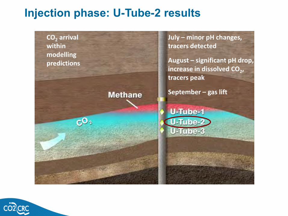
Injection phase: U-Tube-2 results
July – minor pH changes, tracers detected
CO2 arrival within modelling predictions August – significant pH drop,
increase in dissolved CO2, tracers peak
September – gas lift
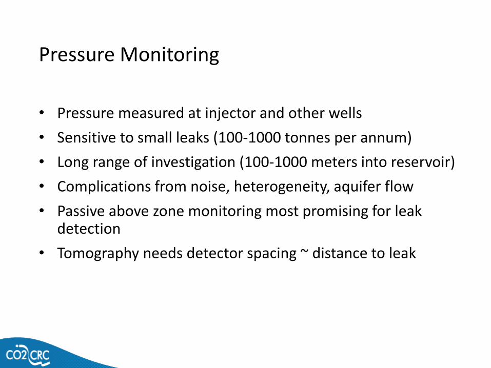
Pressure Monitoring
• Pressure measured at injector and other wells
• Sensitive to small leaks (100-1000 tonnes per annum)
• Long range of investigation (100-1000 meters into reservoir)
• Complications from noise, heterogeneity, aquifer flow
• Passive above zone monitoring most promising for leak detection
• Tomography needs detector spacing ~ distance to leak
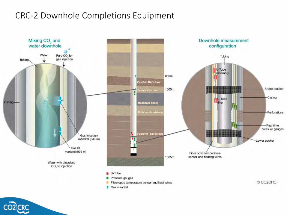
CRC-2 Downhole Completions Equipment
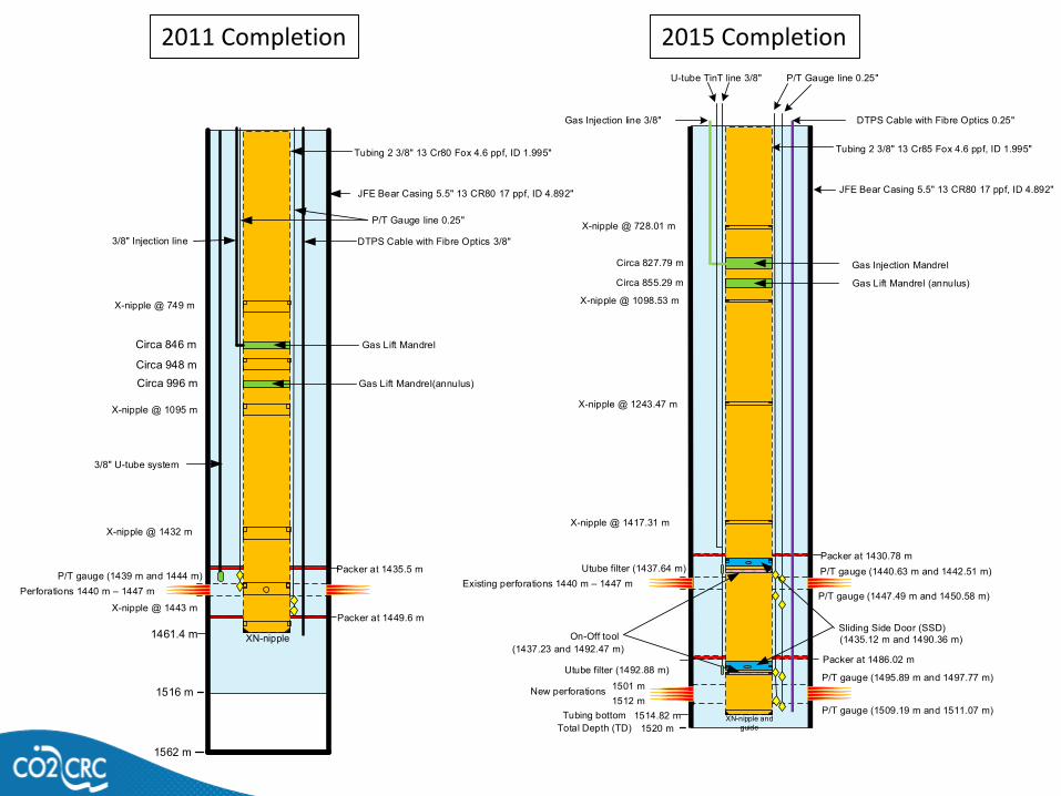
1520 m
(1437.23 and 1492.47 m)
X-nipple @ 1417.31 m
XN-nipple and guide
P/T gauge (1495.89 m and 1497.77 m)
Sliding Side Door (SSD)
Circa 827.79 m
JFE Bear Casing 5.5" 13 CR80 17 ppf, ID 4.892"
Tubing 2 3/8" 13 Cr85 Fox 4.6 ppf, ID 1.995"
Gas Lift Mandrel (annulus)
DTPS Cable with Fibre Optics 0.25"
P/T Gauge line 0.25"
New perforations
P/T gauge (1440.63 m and 1442.51 m)Existing perforations 1440 m – 1447 m
Packer at 1486.02 m
Packer at 1430.78 m
X-nipple @ 1243.47 m
X-nipple @ 1098.53 m
1501 m1512 m
1514.82 mTubing bottom Total Depth (TD)
P/T gauge (1509.19 m and 1511.07 m)
On-Off tool (1435.12 m and 1490.36 m)
P/T gauge (1447.49 m and 1450.58 m)
Gas Injection Mandrel
Circa 855.29 m
Gas Injection line 3/8"
Utube filter (1492.88 m)
Utube filter (1437.64 m)
U-tube TinT line 3/8"
X-nipple @ 728.01 m
1516 m
1461.4 m
X-nipple @ 1432 m
XN-nipple
Circa 996 m
JFE Bear Casing 5.5" 13 CR80 17 ppf, ID 4.892"
Tubing 2 3/8" 13 Cr80 Fox 4.6 ppf, ID 1.995"
Gas Lift Mandrel(annulus)
DTPS Cable with Fibre Optics 3/8"
P/T Gauge line 0.25"
P/T gauge (1439 m and 1444 m)Perforations 1440 m – 1447 m
Packer at 1449.6 m
Packer at 1435.5 m
X-nipple @ 1095 m
X-nipple @ 749 m
X-nipple @ 1443 m
Circa 846 m Gas Lift Mandrel
3/8" Injection line
Circa 948 m
3/8" U-tube system
1562 m
2011 Completion 2015 Completion
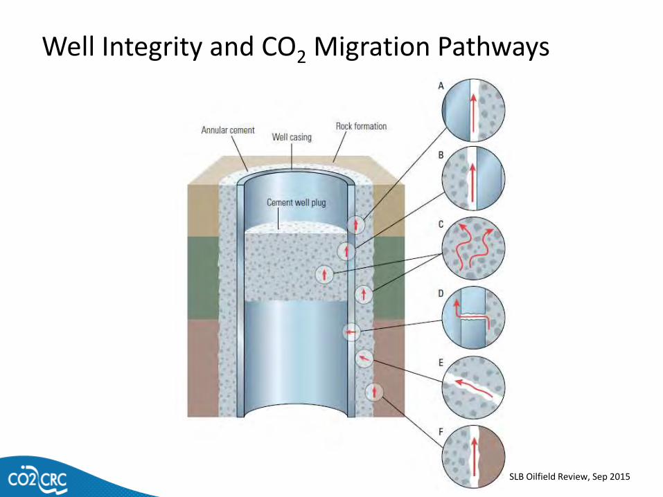
Well Integrity and CO2 Migration Pathways
SLB Oilfield Review, Sep 2015
Deep Monitoring of CO2

Acknowledgements
IndustryANLEC R&D (on behalf of ACALET)
Chevron Australia
Coal 21
Global CCS Institute
INPEX Browse Ltd
Shell Development (Australia) Pty Ltd
CommunityLandowners near site
Moyne Shire
Nirranda South
GovernmentAustralian Government: Department of Education
Australian Government: Department of Industry and Science
CarbonNet Project
NSW: Department of Industry
SA: The Department for Manufacturing, Innovation, Trade, Resources and Energy (DMITRE)
Victoria: Department of Economic Development, Jobs, Transport and Resources
WA: Department of Mines and Petroleum
ResearchAustralian National University
Charles Darwin University
CSIRO
Curtin University
Federation University Australia
Geoscience Australia
GNS Science
Korea Institute of Geosciences & Mineral Resources
Lawrence Berkeley National Laboratory (LBNL)
University of Adelaide
University of Edinburgh
University of Melbourne
University of NSW
University of Queensland
University of Western Australia
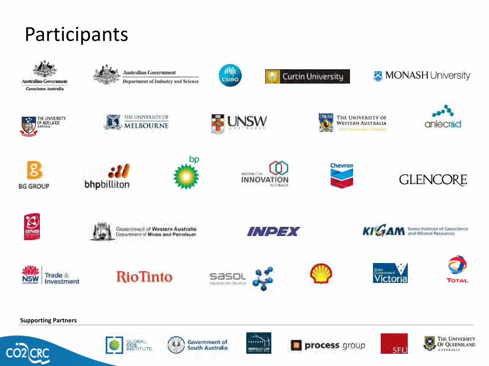
Participants
Supporting Partners