1

Deep Machine Learning: Panel Presentation

Honglak Lee

Computer Science & Engineering Division

University of Michigan

MSR Faculty Summit

7/16/2013

2

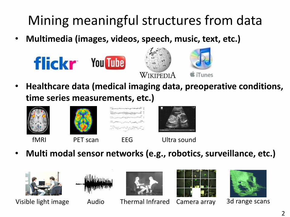
Mining meaningful structures from data • Multimedia (images, videos, speech, music, text, etc.)

• Healthcare data (medical imaging data, preoperative conditions, time series measurements, etc.)

• Multi modal sensor networks (e.g., robotics, surveillance, etc.)

Camera array 3d range scans Visible light image Thermal Infrared Audio

fMRI PET scan Ultra sound EEG

3

Learning Representations

• Key ideas:

– Unsupervised Learning: Learn statistical structure or correlation of the data from unlabeled data (and some labeled data)

– Deep Learning: Learn multiple levels of representation of increasing complexity/abstraction.

– The learned representations can be used as features in supervised and semi-supervised settings.

• I will also talk about how to go beyond supervised (or semi-supervised) problems, such as:

– Weakly supervised learning

– Structured output prediction

4

Natural Images Learned bases: “Edges”

50 100 150 200 250 300 350 400 450 500

50

100

150

200

250

300

350

400

450

500

50 100 150 200 250 300 350 400 450 500

50

100

150

200

250

300

350

400

450

500

50 100 150 200 250 300 350 400 450 500

50

100

150

200

250

300

350

400

450

500

~ 0.8 * + 0.3 * + 0.5 *

x ~ 0.8 * b36 + 0.3 * b42

+ 0.5 * b65

[0, 0, …, 0, 0.8, 0, …, 0, 0.3, 0, …, 0, 0.5, …] = coefficients (feature representation)

Test example

Motivation? Salient features, Compact representation

Compact & easily interpretable

Unsupervised learning with sparsity [NIPS 07; ICML 07; NIPS 08]

5

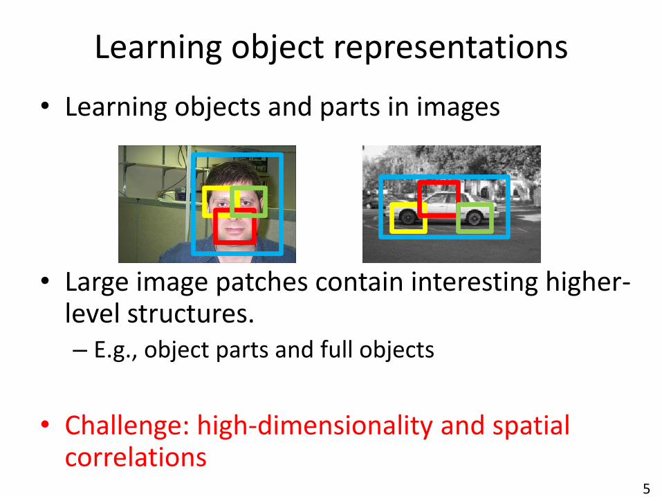
• Learning objects and parts in images

• Large image patches contain interesting higher-level structures. – E.g., object parts and full objects

• Challenge: high-dimensionality and spatial correlations

Learning object representations

6

Example image

“Filtering” output

“Shrink” (max over 2x2)

filter1 filter2 filter3 filter4

“Eye detector” Advantage of shrinking 1. Filter size is kept small 2. Invariance

Illustration: Learning an “eye” detector

7

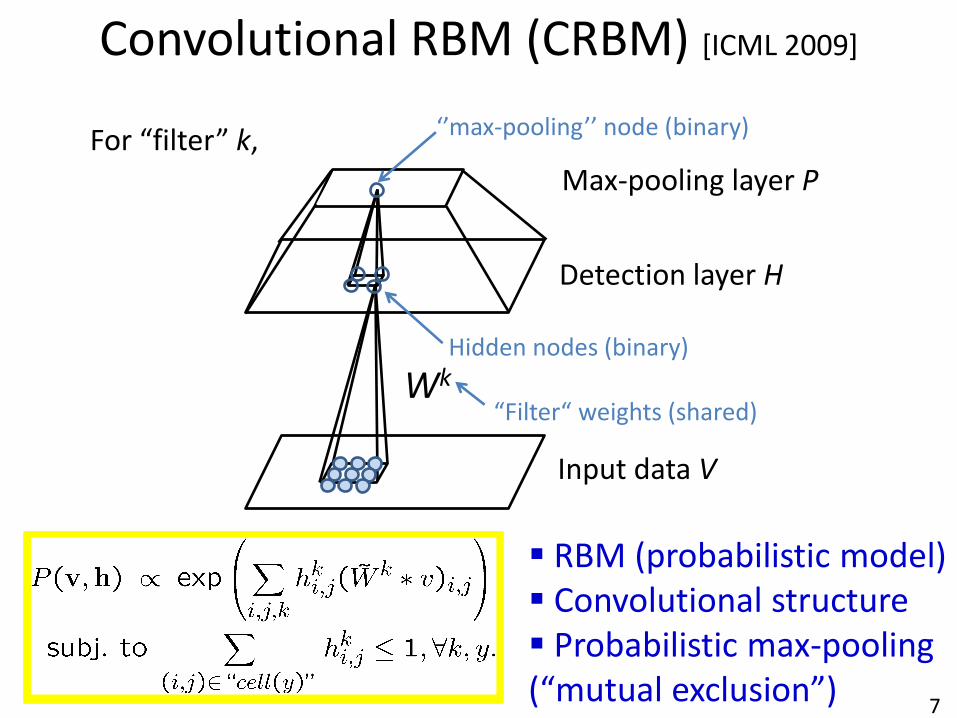
Wk

V (visible layer)

Detection layer H

Max-pooling layer P

Visible nodes (binary or real)

At most one hidden nodes are active.

Hidden nodes (binary)

“Filter“ weights (shared)

For “filter” k, ‘’max-pooling’’ node (binary)

Input data V

Convolutional RBM (CRBM) [ICML 2009]

RBM (probabilistic model) Convolutional structure Probabilistic max-pooling (“mutual exclusion”)

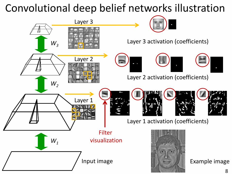
8

W1

W2

W3

Input image

Layer 1

Layer 2

Layer 3

Example image

Layer 1 activation (coefficients)

Layer 2 activation (coefficients)

Layer 3 activation (coefficients)

Show only one figure

Filter visualization

Convolutional deep belief networks illustration

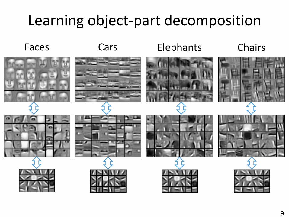
9

Faces Cars Elephants Chairs

Learning object-part decomposition

10

Applications

• Classification (ICML 2009, NIPS 2009, ICCV 2011, Comm.

ACM 2011)

• Verification (CVPR 2012)

• Image alignment (NIPS 2012)

• The algorithm is applicable to other domains, such as audio (NIPS 2009)

11

Ongoing Work

• Investigating theoretical connections and efficient training (ICCV 2011)

• Robust feature learning with weak supervision (ICML 2013)

• Representation learning with structured outputs (CVPR 2013)

• Learning invariant representations (ICML 2009; NIPS 2009; ICML 2012)

• Multi-modal feature learning (ICML 2011)

• Life-long representation learning (AISTAST 2012)

12

Ongoing Work

• Investigating theoretical connections and efficient training (ICCV 2011)

• Robust feature learning with weak supervision (ICML 2013)

• Representation learning with structured outputs (CVPR 2013)

• Learning invariant representations (ICML 2009; NIPS 2009; ICML 2012)

• Multi-modal feature learning (ICML 2011)

• Life-long representation learning (AISTAST 2012)

13

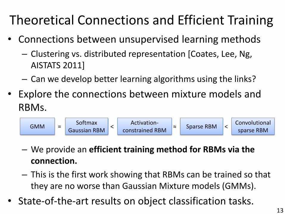
Theoretical Connections and Efficient Training

• Connections between unsupervised learning methods

– Clustering vs. distributed representation [Coates, Lee, Ng, AISTATS 2011]

– Can we develop better learning algorithms using the links?

• Explore the connections between mixture models and RBMs.

– We provide an efficient training method for RBMs via the connection.

– This is the first work showing that RBMs can be trained so that they are no worse than Gaussian Mixture models (GMMs).

• State-of-the-art results on object classification tasks.

GMM Softmax

Gaussian RBM =

Activation-constrained RBM

< Sparse RBM ≈ Convolutional sparse RBM

<

14

Spherical Gaussian Mixtures is equivalent to RBM with softmax constraints

Gaussian Softmax RBM = GMM with shared covariance σ2I

GMM Softmax

Gaussian RBM =

15

Relaxing the constraints

Gaussian Softmax RBM

subj. to ℎ𝑘 ≤ 𝜶𝐾𝑘=1 , activation-constrained RBM

GMM Softmax

Gaussian RBM =

Activation-constrained RBM

<

16

Relaxing the constraints

Gaussian Softmax RBM

subj. to ℎ𝑘 ≤ 𝜶𝐾𝑘=1 , activation-constrained RBM

sparse RBM: (regularize in training) 1

𝐾 ℎ𝑘 ≈

𝛼

𝐾𝐾𝑘=1

GMM Softmax

Gaussian RBM =

Activation-constrained RBM

< Sparse RBM ≈

17

Experiments – Analysis

• Effect of sparsity to the classification performance (Caltech 101).

– The sparsity > 1/K showed the best CV accuracy.

• Practical guarantee that the sparse RBM lead to comparable or better classification performance than Gaussian mixtures.

[ICCV 2011]

18

Ongoing Work

• Investigating theoretical connections and efficient training (ICCV 2011)

• Robust feature learning with weak supervision (ICML 2013)

• Representation learning with structured outputs (CVPR 2013)

• Learning invariant representations (ICML 2009; NIPS 2009; ICML 2012)

• Multi-modal feature learning (ICML 2011)

• Life-long representation learning (AISTAST 2012)

19

Learning from scratch

• Unsupervised feature learning – Powerful in discovering features from unlabeled data.

– However, not all patterns (or data) are equally important. • When data contains lots of distracting factors, learning meaningful

representations can be challenging.

• Feature selection – Powerful in selecting features from labeled data.

– However, it assumes existence of discriminative features. • There may not be such features at hand.

• We develop a joint model for feature learning and feature selection – allows to learn task-relevant high-level features using

(weak) supervision.

20

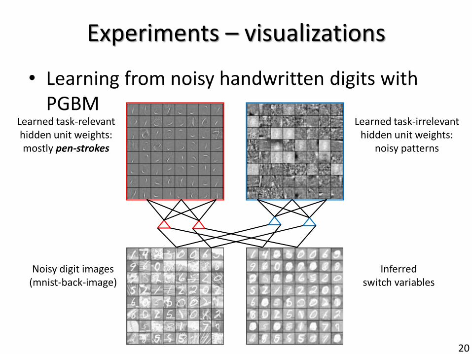
• Learning from noisy handwritten digits with PGBM

Experiments – visualizations

Learned task-relevant hidden unit weights: mostly pen-strokes

Inferred switch variables

Noisy digit images (mnist-back-image)

Learned task-irrelevant hidden unit weights:

noisy patterns

21

• Learning from noisy handwritten digits with PGBM

Experiments – visualizations

Learned task-relevant hidden

unit weights: mostly pen-strokes

Inferred switch variables

Noisy digit images

(mnist-back-image)

Learned task-irrelevant hidden unit

weights: noisy patterns

y

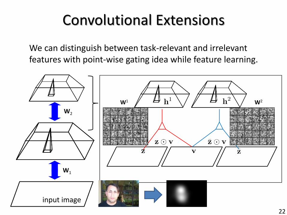
22

We can distinguish between task-relevant and irrelevant features with point-wise gating idea while feature learning.

Convolutional Extensions

input image

W1

W2

W1 W2

23

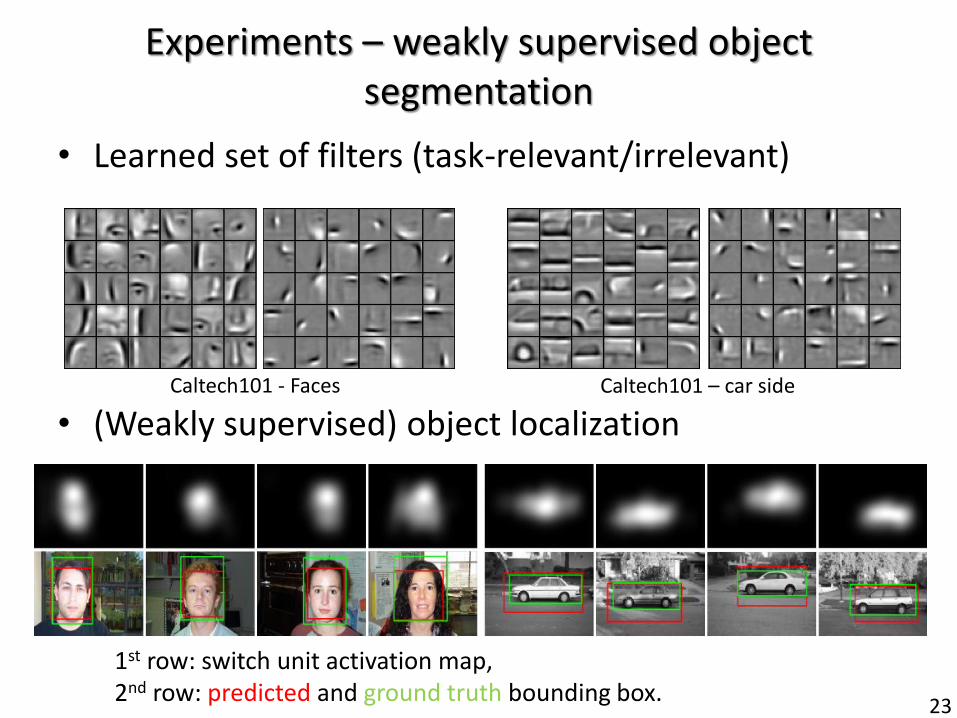
• Learned set of filters (task-relevant/irrelevant)

• (Weakly supervised) object localization

Experiments – weakly supervised object segmentation

Caltech101 - Faces Caltech101 – car side

1st row: switch unit activation map, 2nd row: predicted and ground truth bounding box.

24

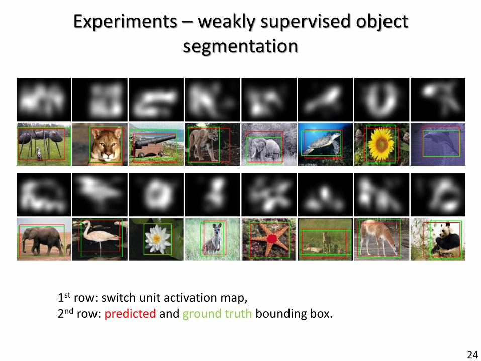
Experiments – weakly supervised object segmentation

1st row: switch unit activation map, 2nd row: predicted and ground truth bounding box.

25

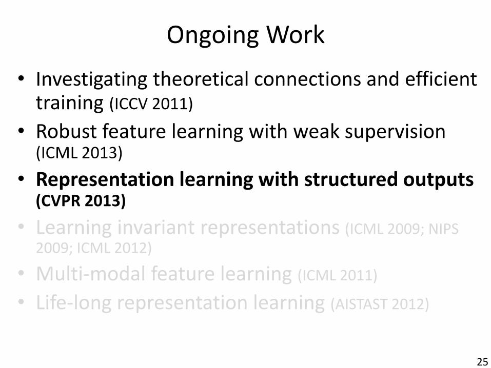
Ongoing Work

• Investigating theoretical connections and efficient training (ICCV 2011)

• Robust feature learning with weak supervision (ICML 2013)

• Representation learning with structured outputs (CVPR 2013)

• Learning invariant representations (ICML 2009; NIPS 2009; ICML 2012)

• Multi-modal feature learning (ICML 2011)

• Life-long representation learning (AISTAST 2012)

26

Enforcing Global and Local Consistencies for Structured Output Prediction

• Task: scene segmentation

• Problem: only enforces local consistency

• Our model can enforce both local and global consistency

Image Over-segmentation Target Output

CRF with superpixels

s

(CVPR 2013)

27

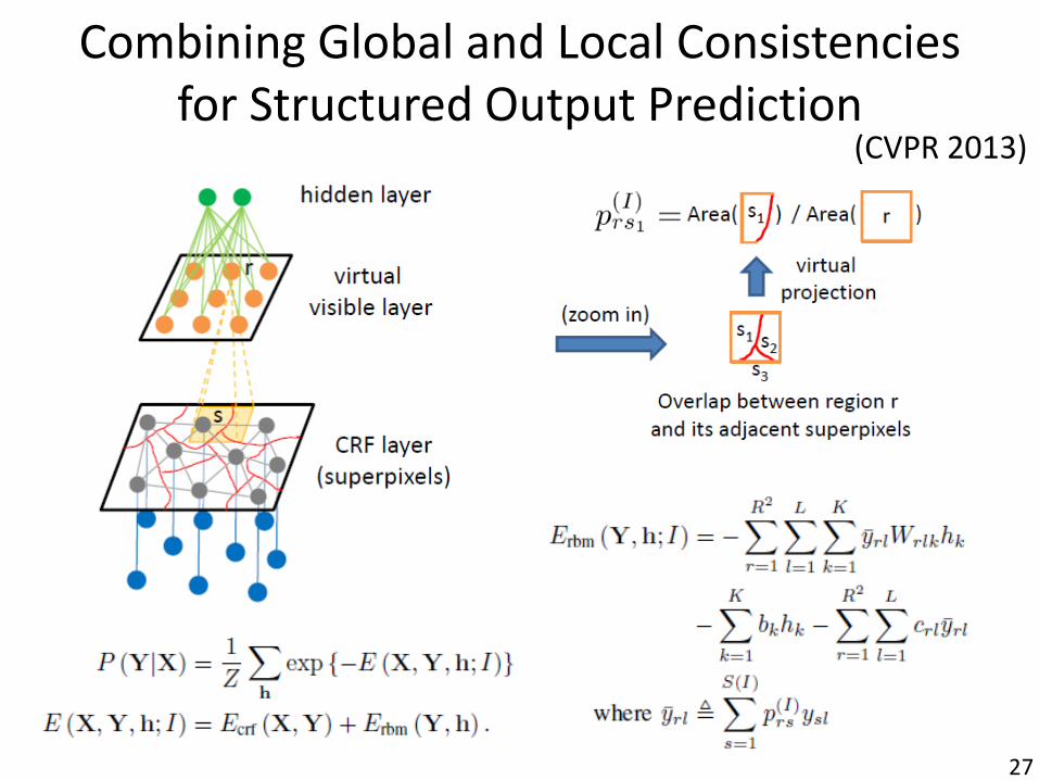
Combining Global and Local Consistencies for Structured Output Prediction

(CVPR 2013)

28

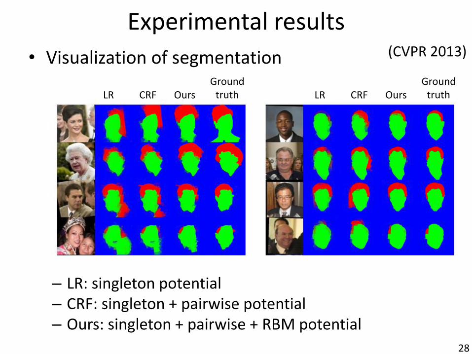
Experimental results

• Visualization of segmentation

– LR: singleton potential – CRF: singleton + pairwise potential – Ours: singleton + pairwise + RBM potential

LR CRF Ours Ground

truth LR CRF Ours Ground

truth

(CVPR 2013)

29

Summary

• Generative learning of convolutional feature hierarchy

• Better training algorithms

• Learning representations with weak supervision

• Learning representations with structured outputs

Funding support:

– NSF, ONR, Google, Toyota, Bosch Research