Data analysis lecture
119
Advanced Bioprocess Engineering Data Analysis & Design of Experiments Dr. Ir. Eirini Velliou 22 February 2013 © Imperial College London
Transcript of Data analysis lecture
Advanced Bioprocess Engineering
Data Analysis &
Design of Experiments
Dr. Ir. Eirini Velliou 22 February 2013
© Imperial College London
© Imperial College London Page 2
Good Research Planning Step by step
• Which are the specific objectives of the experiment?
• Which are the influential factors ? Which of those factors to vary ? Which to hold constant ?
• Which are the characteristics to be measured ?
• Which are the specific procedures for conducting tests or measuring the characteristics?
• Which is the number of repetitions of the basic experiment to conduct ?
• Which are the available resources and materials?

© Imperial College London Page 3
Statistics-Step by Step
• Data Collection
• Summarizing Data
• Interpreting Data
• Drawing Conclusions from Data
© Imperial College London Page 4
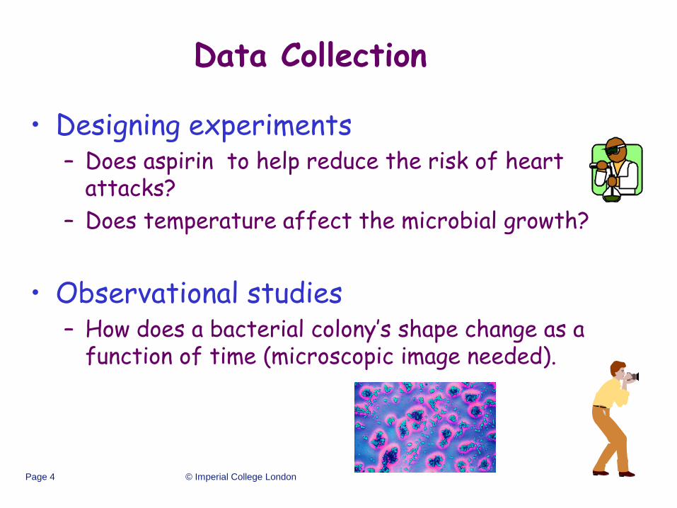
Data Collection
• Designing experiments – Does aspirin to help reduce the risk of heart
attacks?
– Does temperature affect the microbial growth?
• Observational studies – How does a bacterial colony’s shape change as a
function of time (microscopic image needed).

© Imperial College London Page 5

© Imperial College London Page 6
Population The set of data (numerical or otherwise)
corresponding to the entire collection of units about
which information is sought.
Sample
A subset of the population data that are actually collected in the course of a study.

© Imperial College London Page 7
Population vs. Sample
Population Sample

© Imperial College London Page 8
WHY? In most studies, it is difficult
to obtain information from the entire population. We rely on samples to make estimates or inferences related to the population.
Population vs. Sample

© Imperial College London Page 9
Data classification
Data types
Continuous Discrete
Qualitative (Categorical)
Quantitative (numerical)
Discrete

© Imperial College London Page 10

© Imperial College London Page 11
What to describe?
• What is the “location” or “center” of the data? (“measures of location”)
• How do the data vary? (“measures of variability”)

© Imperial College London Page 12
Measures of Location
• Mean
• Median
• Mode

© Imperial College London Page 13
Mean
• Another name for average.
• If describing a population, it is denoted as , the greek letter “mu”.
• If describing a sample, denoted as “x-bar”.
• Appropriate for describing measurement data.
• Seriously affected by unusual values called “outliers”.

© Imperial College London Page 14
Calculation of a sample mean
ni
XX
Formula:
That is, add up all of the data points and divide by the number of data points.
Data (# of classes skipped): 2 8 3 4 1
Sample Mean = (2+8+3+4+1)/5 = 3.6
Do not round! Mean need not be a whole number.
© Imperial College London Page 15
Median
• Another name for 50th percentile.
• Appropriate for describing measurement data.
• “Robust to outliers,” that is, not affected much by unusual values.

© Imperial College London Page 16
Calculation of a sample median
Order data from smallest to largest.
If odd number of data points, the median is the middle value.
Data (# of classes skipped): 2 8 3 4 1
Ordered Data: 1 2 3 4 8
Median

© Imperial College London Page 17
Calculating Sample Median
Order data from smallest to largest.
If even number of data points, the median is the average of the two middle values.
Data (# of classes skipped): 2 8 3 4 1 8
Ordered Data: 1 2 3 4 8 8
Median = (3+4)/2 = 3.5

© Imperial College London Page 18
Most appropriate measure of location
• Depends on whether or not data are “symmetric” or “skewed”.
• Depends on whether or not data have one (“unimodal”) or more (“multimodal”) modes.

© Imperial College London Page 19
Symmetric and Unimodal
2.0 2.2 2.4 2.6 2.8 3.0 3.2 3.4 3.6 3.8 4.0
0
10
20
GPAs
Perc
ent

© Imperial College London Page 20
Symmetric and Bimodal

© Imperial College London Page 21
Symmetric and Bimodal

© Imperial College London Page 22
Skewed Right
0 100 200 300 400
0
10
20
Number of Music CDs
Fre
quency
Number of Music CDs of Spring 1998 Stat 250 Students
© Imperial College London Page 23
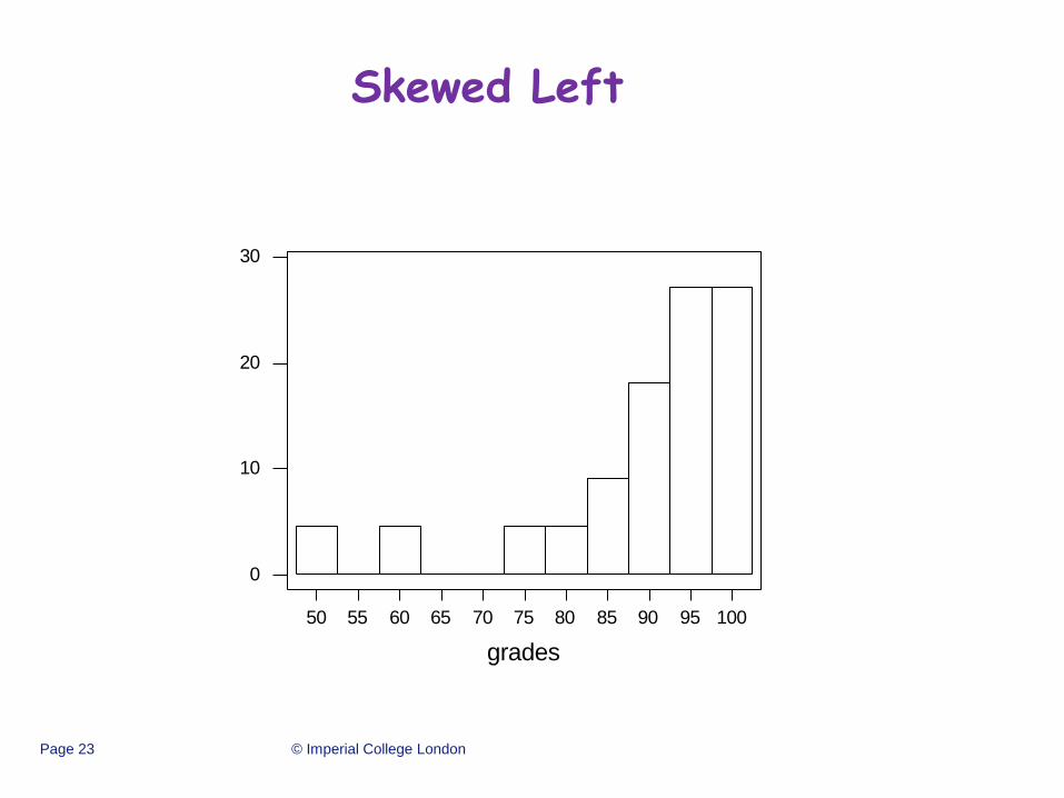
Skewed Left
50 55 60 65 70 75 80 85 90 95 100
0
10
20
30
grades
Perc
ent

© Imperial College London Page 24
Choosing Appropriate Measure of Location
• If data are symmetric, the mean, median, and mode will be approximately the same.
• If data are multimodal, report the mean, median and/or mode for each subgroup.
• If data are skewed, report the median.

© Imperial College London Page 25
Measures of Variability
• Range
• Variance and standard deviation
• Coefficient of variation
All of these measures are appropriate for measurement data only.

© Imperial College London Page 26
Range
• The difference between largest and smallest data point.
• Highly affected by outliers.
• Best for symmetric data with no outliers.

© Imperial College London Page 27
What is the range?
2.0 2.2 2.4 2.6 2.8 3.0 3.2 3.4 3.6 3.8 4.0
0
10
20
GPA
Fre
quency
GPAs of Spring 1998 Stat 250 Students

© Imperial College London Page 28
Range
Descriptive Statistics
Variable N Mean Median TrMean StDev SE Mean
GPA 92 3.0698 3.1200 3.0766 0.4851 0.0506
Variable Minimum Maximum Q1 Q3
GPA 2.0200 3.9800 2.6725 3.4675
Range = 3.98 - 2.02 = 1.96

© Imperial College London Page 29
Variance
1n
2)x(x2s
1. Find difference between each data point and mean.
2. Square the differences, and add them up.
3. Divide by one less than the number of data points.

© Imperial College London Page 30
Variance
• If measuring variance of population, denoted by 2 (“sigma-squared”).
• If measuring variance of sample, denoted by s2 (“s-squared”).
• Measures average squared deviation of data points from their mean.
• Highly affected by outliers. Best for symmetric data.
• Problem is units are squared.

© Imperial College London Page 31
Standard deviation
• Sample standard deviation is square root of sample variance, and so is denoted by s.
• Units are the original units.
• Measures average deviation of data points from their mean.
• Also, highly affected by outliers.

© Imperial College London Page 32
What is the variance or standard deviation?
70 80 90 100 110 120 130 140 150 160
Speed
Fastest Ever Driving Speed
126
Women
100
Men
226 Stat 100 Students, Fall '98
(MPH)

© Imperial College London Page 33
Coefficient of variation (MPH)
Sex N Mean Median TrMean StDev SE Mean
female 126 91.23 90.00 90.83 11.32 1.01
male 100 106.79 110.00 105.62 17.39 1.74
Minimum Maximum Q1 Q3
female 65.00 120.00 85.00 98.25
male 75.00 162.00 95.00 118.75
Females: CV = (11.32/91.23) x 100 = 12.4
Males: CV = (17.39/106.79) x 100 = 16.3
© Imperial College London Page 34
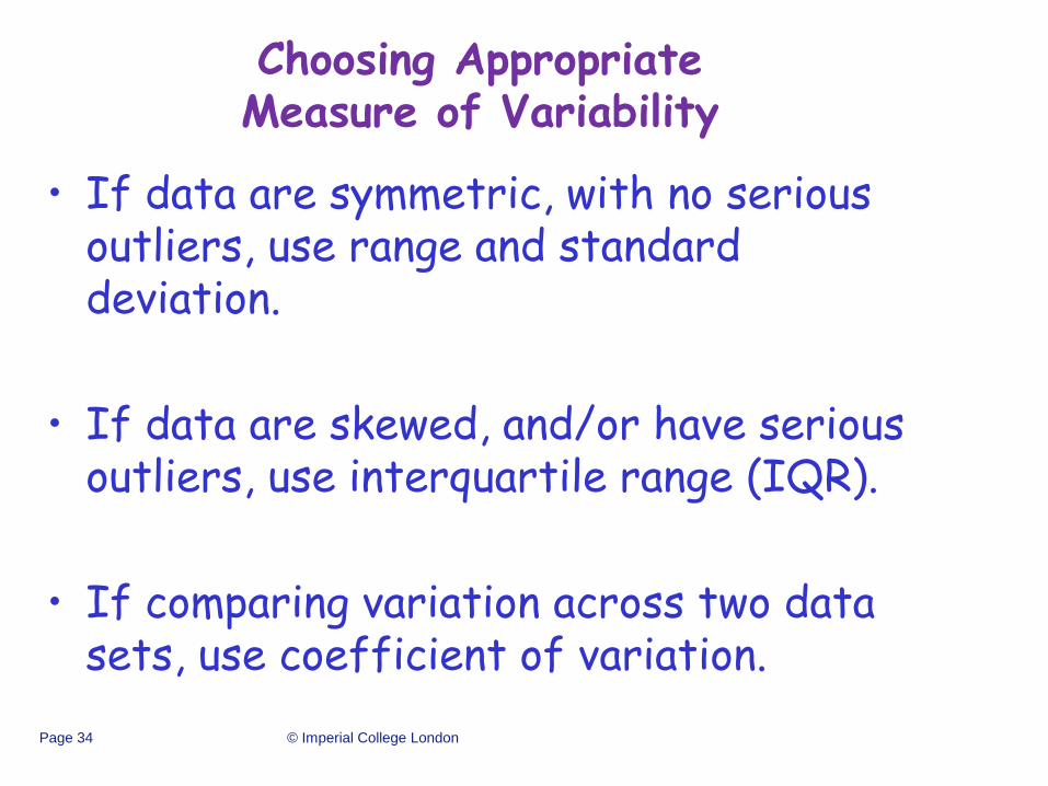
Choosing Appropriate Measure of Variability
• If data are symmetric, with no serious outliers, use range and standard deviation.
• If data are skewed, and/or have serious outliers, use interquartile range (IQR).
• If comparing variation across two data sets, use coefficient of variation.

© Imperial College London Page 35
Sample Variance
s
x x
n
i
i
n
2
2
1
1
Sample Standard Deviation
s s
x x
n
i
i
n
2
2
1
1

Measures of Variation - Some Comments
• Range is the simplest, but is very sensitive to outliers
• Variance units are the square of the original units
• Interquartile range is mainly used with skewed data (or data with outliers)
• We will use the standard deviation as a measure of variation often in this course

© Imperial College London Page 37
4 Common Sense Things
• Random sample good, we use
• Statistics have error
• Statistics have distributions
• Larger sample size (n) is better - less error
30n
© Imperial College London Page 38
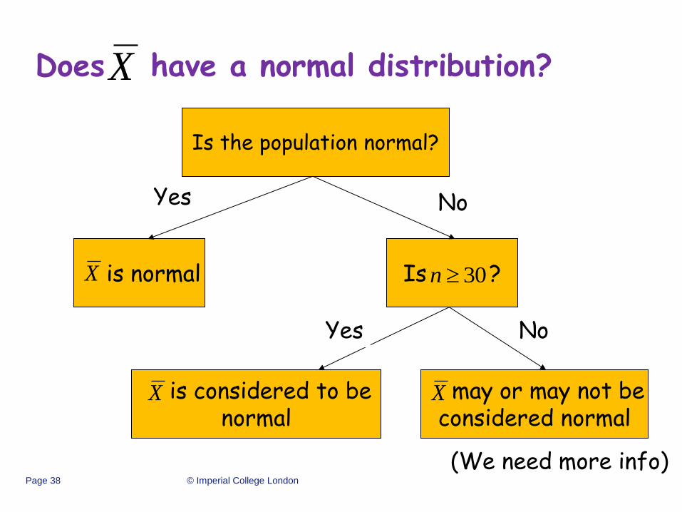
Does have a normal distribution? X
Is the population normal?
is normal Is ?
may or may not be considered normal
X
is considered to be normal
X
30n
X
(We need more info)
Yes
Yes
No
No

© Imperial College London Page 39

© Imperial College London Page 40
Comparison of Five Tire Brands Stopping Distance at 60 mph
180 190 200 210
1
2
3
4
5
Distance (feet)
Bra
nd
Brand N MEAN SD
1 10 188.20 3.88
2 10 195.20 9.02
3 10 187.40 5.27
4 10 191.20 5.55
5 10 200.50 5.44

© Imperial College London Page 41
1-way ANOVA Hypotheses
• The null hypothesis is that the group population means are all the same. That is: – H0: 1 = 2 = 3 = 4 = 5
• The alternative hypothesis is that at least one group population mean differs from the others. That is: – HA: at least one i differs from the others
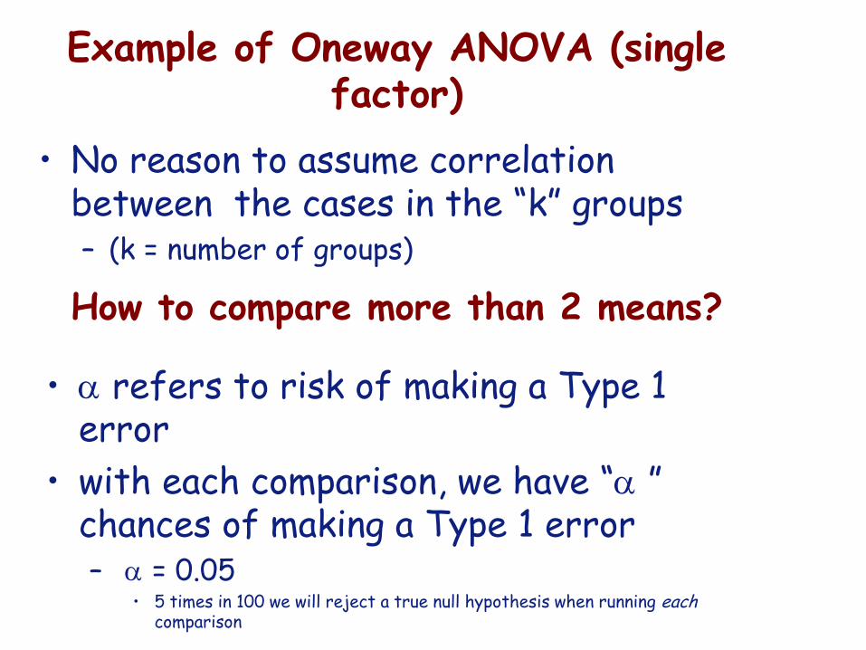
Example of Oneway ANOVA (single factor)
• No reason to assume correlation between the cases in the “k” groups – (k = number of groups)
How to compare more than 2 means?
• refers to risk of making a Type 1 error
• with each comparison, we have “ ” chances of making a Type 1 error – = 0.05
• 5 times in 100 we will reject a true null hypothesis when running each comparison

Type 1 error rate is exponentially cumulative
Family Wise error rate
FW = 1- (1 - )c
where c is the number of
comparisons to be made if = 0.05 and c=3

Type 1 error rate is exponentially cumulative
Family Wise error rate with 3 means to compare
FW = 1- (1 - 0.05)3 = 0.143
Note: always overestimates the error rate ie if = 0.05: k = 3; k = 4?????

ANOVA
an attempt to maintain the FW error rate at a known (acceptable) level

Steps to Oneway ANOVA
• set (0.05)
• set sample size – Example: Thirty randomly selected subjects
• Three randomly assigned groups
– n = 10 in each group • Grp 1: Regular Diet
• Grp 2: CHO supp diet (0.5 g/kg)
• Gpr 3: CHO supp diet (1.0 g/kg)
• set HO:

Set statistical hypothesis: I
HO • Null hypothesis
– Any observed difference between the 3 groups will be attributable to random sampling errors
H1 (HA) • Alternative
hypothesis – If HO is rejected, the
difference is not attributable to random sampling errors (for exampleperhaps diet)?

Set statistical hypotheses: II
• HO • Null hypothesis
– The population means of the 3 groups are equal
• H1 • Alternative
hypothesis – The population means
of the three groups differ in some way Note: no directional hypothesis; Null may be false in many different ways

Analytical Steps
• Set (0.05)
• set sample size
• set Ho
• test all subjects with a standardized protocol

EXAMPLE
file ANOVA1.sav
Steps
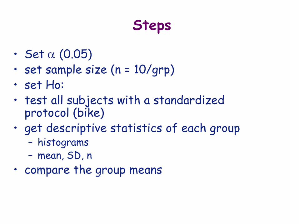
• Set (0.05) • set sample size (n = 10/grp) • set Ho: • test all subjects with a standardized
protocol (bike) • get descriptive statistics of each group
– histograms – mean, SD, n
• compare the group means
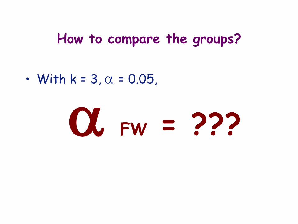
How to compare the groups?
• With k = 3, = 0.05,
FW = ???

Concept of ANOVA
• Evaluate the effect of treatment by analyzing the amount of variation among the subgroup sample means
But how much variation is expected
if the subgroup population means are
equal?

Some Nomenclature
• Grand Mean: mean of all scores, regardless of group – ie all 30 scores
• Group Mean: mean of all scores from subjects treated the same – groups of 10 X
X

3 Sources of Variability (Deviation Scores!!!!)
X - X
X - X
X - X
: Total Variability (Total Sum of Squares)
: Within Group Variability
(within Group Sum of Squares)
: Between Group Variability
(between Groups Sum of Squares)

3 Sources of Variability (Deviation Scores!!!!)
X - X
X - X
X - X
Degrees of freedom (df)=
number of values that are free
to vary in the final calculation
of statistics
df for EACH group = n-1
df for TOTAL groups = k (n-1)

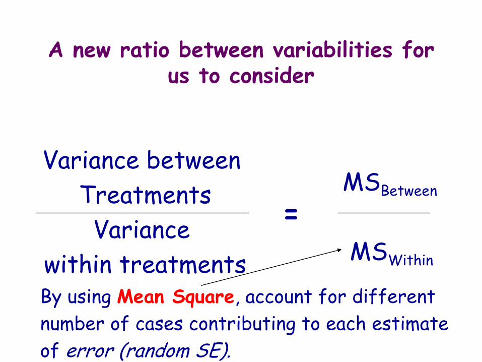
A new ratio between variabilities for us to consider
Variance between
Treatments
Variance
within treatments
= MSBetween
MSWithin
Between= between group variability
Within= within group variability
A new ratio between variabilities for us to consider
Variance between
Treatments
Variance
within treatments
= MSBetween
MSWithin
By using Mean Square, account for different
number of cases contributing to each estimate
of error (random SE).

A new ratio between variabilities for us to consider
= MSBetween
MSWithin
Note: if Treatment effect = 0 (ie no effect)
the ratio will be equal to 1.00
F

Evaluating Fobserved with the F distribution
• A distribution of F ratios is not normally distributed
• follows an F distribution – positively skewed
– depends on the number of degrees of freedom in the numerator (MS between) and the denominator (MS within)

The F distribution (hypothetical)
0 1 2 3 4 5 6 7 8

Fcritical : the F value that
must be equaled or
exceeded to classify a
difference among group
means as statistically
significant (identify a
main effect)

Fcritical depends on df of MSbetween and MS within, and chosen
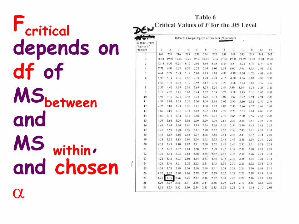
Fcritical depends on df of MSbetween and MS within, and chosen

The F distribution (hypothetical)
Region of rejection
0 1 2 3 4 5 6 7 8
F.05 = ???
For our Diet study, with = 0.05 and df = 2 and 27, Fcritical = ???

The F distribution (hypothetical)
F distribution for df 2, 27

Concept of evaluating Fobs against Fcrit
Area = 0.05 (5%)
Fcrit = 3.35
F distribution for df 2, 27

Concept of evaluating Fobs against Fcrit
Area = 0.05 (5%)
Fcrit = 3.35
Fobs < Fcrit, Decision: ?????
F distribution for df 2, 27

Concept of evaluating Fobs against Fcrit
Area = 0.05 (5%)
Fcrit = 3.35
Fobs Fcrit, Decision: ?????
F distribution for df 2, 27
Running Oneway ANOVA (single factor ANOVA)
Using SPSS
Demonstrate with anova1.sav
3 8 .9 03 .5 4
4 4 .2 02 .8 6
4 4 .7 02 .6 7
F a tigue T im e (M ins )N o rm a l
F a tigue T im e (M ins )0 .5 g C H O
F a tigue T im e (M ins )1 .0 g C H O
M e a nS td D e v ia tio n

1-way ANOVA in SPSS
Procedure: Choose the appropriate procedure,
and…

1-way ANOVA in SPSS
Dialog box: slide the variables…
…into the appropriate places

ANOVA in SPSS
ANO VA
Fatigue T im e (M ins)
206.6002103.30011.130.000
250.600279.281
457.20029
Betw een G roups
W ithin G roups
Tota l
Sum of
SquaresdfM ean SquareFS ig .
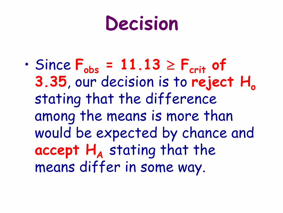
Decision
• Since Fobs = 11.13 Fcrit of 3.35, our decision is to reject Ho stating that the difference among the means is more than would be expected by chance and accept HA stating that the means differ in some way.

© Imperial College London Page 75

© Imperial College London Page 76
Experiment
• A widely used approach for data collection
• Widely used in science and industry
• The primary goal of experiment in scientific research is usually to show the statistical significance of an effect that a particular factor exerts on the dependent variable of interest

© Imperial College London Page 77
Experiment
• Experiment is “a test or series of tests in which purposeful changes are made to the input variables of a process or system so that we may observe and identify the reasons for changes that may be observed in the output response”. (Montgomery 2009)

© Imperial College London
Experiment
• Traditional approach • (Dose-response method)
• Trial and Error • One-factor-at-a-time experiments
laborious, slow, time and cost consuming since it can test limited no. of factors at a time and do not allow the investigation of how a factor affects a product or process in the presence of other factors (ignore interactions) and may lead to incorrect conclusions

© Imperial College London Page 79
Design of Experiment (DoE)
• Statistical analytical approach
• can test multiple variables and parameters at a time.
• Run less experiments and decrease the resources
• Ensures that all factors and their interactions are symmetrically investigated.
• Find Robust solutions
• Find Optimal conditions
• Complete and reliable information

© Imperial College London
DoE
• Design of Experiments: A branch of applied statistics dealing with planning, conducting, analyzing, and interpreting controlled tests to evaluate the factors that control the value of a parameter or group of parameters.
• Selected from Donna C. S. Summers, Quality, 2nd Ed. (2000), Prentice Hall: Upper SaddleRiver, New Jersey, page 625

© Imperial College London Page 81
Statistical terms: Factors
Factors – experimental factors or independent variables (continuous or discrete) an investigator manipulates to capture any changes in the output of the process. Other factors of concern are those that are uncontrollable and those which are controllable but held constant during the experimental runs.

© Imperial College London Page 82
Statistical terms: Response
Responses –
dependent variable measured to describe the output of the process.
© Imperial College London Page 83
Statistical terms: Treatment
Treatment Combinations (run) – experimental trial where all factors are set at a specified level.
© Imperial College London Page 84
Statistical terms: Replication
Replication –
repetition of a basic experiment without changing any factor settings, allows the experimenter to estimate the experimental error (noise) in the system used to determine whether observed differences in the data are “real” or “just noise”, allows the experimenter to obtain more statistical power (ability to identify small effects)

© Imperial College London Page 85
Statistical terms: Randomization
Randomization –
a statistical tool used to minimize potential uncontrollable biases in the experiment by randomly assigning material, people, order that experimental trials are conducted, or any other factor not under the control of the experimenter. Results in “averaging out” the effects of the extraneous factors that may be present in order to minimize the risk of these factors affecting the experimental results.

© Imperial College London Page 86
Statistical terms: Blocking
Blocking –
technique used to increase the precision of an experiment by breaking the experiment into homogeneous segments (blocks) in order to control any potential block to block variability (multiple lots of raw material, several shifts, several machines, several inspectors). Any effects on the experimental results as a result of the blocking factor will be identified and minimized.

© Imperial College London Page 87
DOE STEPS
• Problem statement
• Choice of factors, levels, and ranges
• Choice of response variable (s)
• Choice of experimental design
• Performing the experiment
• Statistical analysis
• Conclusions and recommendations
© Imperial College London Page 88
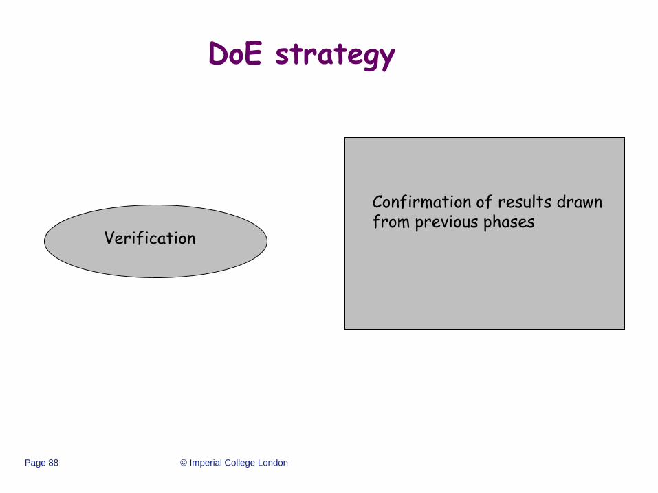
DoE strategy
Screening Characterization Optimization Verification
This phase explores the effects
of a large number of variables,
with the objective of identifying
a smaller number of variables to
study further in characterization
or optimization experiments.
Follow-up experiment that
focuses on the few vital factors,
this will provide better
understanding of
system/process by estimating
interactions and main effects.
Develop a predictive model for
the system that can be used to
find useful operating
conditions.
Confirmation of results drawn from previous phases

© Imperial College London Page 89
Screening Designs
• Tools: 1. Two-level full factorial
design
2. Two-level fractional factorial design
3. Mixture Design
4. Plackett-Burman Design
5. Taguchi Designs
• To identify the most significant factors that affect the process under investigation using the fewest number of trials or experiments.
© Imperial College London Page 90
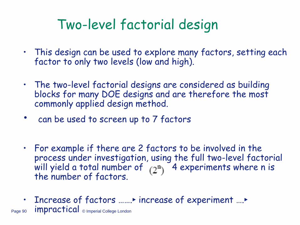
Two-level factorial design
• This design can be used to explore many factors, setting each factor to only two levels (low and high).
• The two-level factorial designs are considered as building blocks for many DOE designs and are therefore the most commonly applied design method.
• can be used to screen up to 7 factors
• For example if there are 2 factors to be involved in the process under investigation, using the full two-level factorial will yield a total number of 4 experiments where n is the number of factors.
• Increase of factors …….► increase of experiment ….► impractical

(Full) Factorial Designs
• All possible combinations of the factor
settings
• Two-level designs: 2 x 2 x 2 …
• General: I x J x K … combinations


9.5
5.5


Algebra
-1 x -1 = +1
…


Full Factorial Design
Design Matrix

9 + 9 + 3 + 3 6
7 + 9 + 8 + 8 8
6 – 8 = -2
7
9
9
9
8
3
8
3


Fractional Factorial Designs
• Why?
• What?
• How?
• Properties

Treatment combinations
Why Fractional Factorials?
Full Factorials
No. of combinations
This is only for
two-levels

How to select a subset of 4 runs
from a -run design?
Many possible “fractional” designs

Here’s one choice

Need a principled approach!
Here’s another …

Need a principled approach for selecting FFD’s
Regular Fractional Factorial Designs
Wow!
Balanced design
All factors occur and low and high levels
same number of times; Same for interactions.
Columns are orthogonal. Projections …
Good statistical properties

© Imperial College London Page 112
Example : Experimental Results
DESIGN-EXPERT PlotTCN
A: Wnt-3B: BMP-4C: ShhD: Ang-1E: Anglp-3F: IGF-1-IIG: FGF-IH: STF
Half Normal plot
Half N
ormal
% pro
babili
ty
|Effect|
0.00 6.60 13.19 19.79 26.38
0
20
40
60
70
80
85
90
95
97
99
B
H
AD

© Imperial College London Page 113
Example: Experimental Results- Interaction Graph
DESIGN-EXPERT Plot
Response 1
X = A: AY = D: D
Design Points
D- -1.000D+ 1.000
Actual FactorsB: B = 0.00C: C = 0.00E: E = 0.00F: F = 0.00G: G = 0.00H: H = 0.00
D: D
Interaction Graph
Res
pons
e 1
A: A
-1.00 -0.50 0.00 0.50 1.00
0.33
11.1625
21.995
32.8275
43.66

© Imperial College London Page 114
Fractional Factorial Design
• Only a fraction of the full design is used to perform the
screening.
• The main and interactive effects are aliased with each other
leading to a reduction in the number of experiment based on the assumption that higher-order interactions are often negligible.
• The effectiveness of the fractional factorial design depends on the resolution of the design which are defined as
resolution III, IV, and V.

“resolution” ability to separate main effects from low order interactions

Resolution
Resolution III: (1+2)
Main effect aliased with 2-order interactions
Resolution IV: (1+3 or 2+2)
Main effect aliased with 3-order interactions and
2-factor interactions aliased with other 2-factor …
Resolution V: (1+4 or 2+3)
Main effect aliased with 4-order interactions and
2-factor interactions aliased with 3-factor interactions

How to choose appropriate design?
Software for a given set of generators, will give design, resolution, and aliasing relationships
SAS, JMP, Minitab, …
Resolution III designs easy to construct but main effects are aliased with 2-factor interactions
Resolution V designs also easy but not as economical
(for example, 6 factors need 32 runs)
Resolution IV designs most useful but some two-factor interactions are aliased with others.

© Imperial College London Page 118
Fractional Factorial Design
• Generally, the higher resolution design is considered a more thorough design
© Imperial College London Page 119
References
• Design-Ease® Software User’s Guide. Version 6. Stat-Ease®, Inc., 2000.
• Design of Experiments: Case Studies & Articles. Stat-Ease®, Inc. 8 Aug.2003. <http://www.statease.com/articles.html>.
• Montgomery, Douglas C. Design and Analysis of Experiments, 3rd edition. New York: John Wiley & Sons, 1991.


![Lecture 4 BJT Small Signal Analysis01 [??????????????????]pws.npru.ac.th/thawatchait/data/files/Lecture 4 BJT Small... · 2016-09-12 · Lecture 4 BJJg yT Small Signal Analysis Present](https://static.fdocument.pub/doc/165x107/5e674360ee8da93175055e37/lecture-4-bjt-small-signal-analysis01-pwsnpruacththawatchaitdatafileslecture.jpg)